scientiﬁc computing: an introductory...

IntroductionApproximations

Computer ArithmeticMathematical Software

Scientific Computing: An Introductory SurveyChapter 1 – Scientific Computing

Prof. Michael T. Heath

Department of Computer ScienceUniversity of Illinois at Urbana-Champaign

Copyright c© 2002. Reproduction permittedfor noncommercial, educational use only.

Michael T. Heath Scientific Computing 1 / 50



Outline

1 Introduction

2 Approximations

3 Computer Arithmetic

4 Mathematical Software




Scientific Computing

What is scientific computing?

Design and analysis of algorithms for numerically solvingmathematical problems in science and engineeringTraditionally called numerical analysis

Distinguishing features of scientific computing

Deals with continuous quantitiesConsiders effects of approximations

Why scientific computing?

Simulation of natural phenomenaVirtual prototyping of engineering designs




Well-Posed Problems

Problem is well-posed if solutionexistsis uniquedepends continuously on problem data

Otherwise, problem is ill-posed

Even if problem is well posed, solution may still besensitive to input data

Computational algorithm should not make sensitivity worse




General Strategy

Replace difficult problem by easier one having same orclosely related solution

infinite → finitedifferential → algebraicnonlinear → linearcomplicated → simple

Solution obtained may only approximate that of originalproblem




Sources of Approximation

Before computationmodelingempirical measurementsprevious computations

During computationtruncation or discretizationrounding

Accuracy of final result reflects all these

Uncertainty in input may be amplified by problem

Perturbations during computation may be amplified byalgorithm




Example: Approximations

Computing surface area of Earth using formula A = 4πr2

involves several approximations

Earth is modeled as sphere, idealizing its true shape

Value for radius is based on empirical measurements andprevious computations

Value for π requires truncating infinite process

Values for input data and results of arithmetic operationsare rounded in computer




Absolute Error and Relative Error

Absolute error : approximate value − true value

Relative error : (absolute error) / (true value)

Equivalently, approx value = (true value) × (1 + rel error)

True value usually unknown, so we estimate or bounderror rather than compute it exactly

Relative error often taken relative to approximate value,rather than (unknown) true value




Data Error and Computational Error

Typical problem: compute value of function f : R → R forgiven argument

x = true value of inputf(x) = desired resultx = approximate (inexact) inputf = approximate function actually computed

Total error: f(x)− f(x) =

f(x)− f(x) + f(x)− f(x)computational error + propagated data error

Algorithm has no effect on propagated data error




Truncation Error and Rounding Error

Truncation error : difference between true result (for actualinput) and result produced by given algorithm using exactarithmetic

Due to approximations such as truncating infinite series orterminating iterative sequence before convergence

Rounding error : difference between result produced bygiven algorithm using exact arithmetic and result producedby same algorithm using limited precision arithmetic

Due to inexact representation of real numbers andarithmetic operations upon them

Computational error is sum of truncation error androunding error, but one of these usually dominates




Example: Finite Difference Approximation

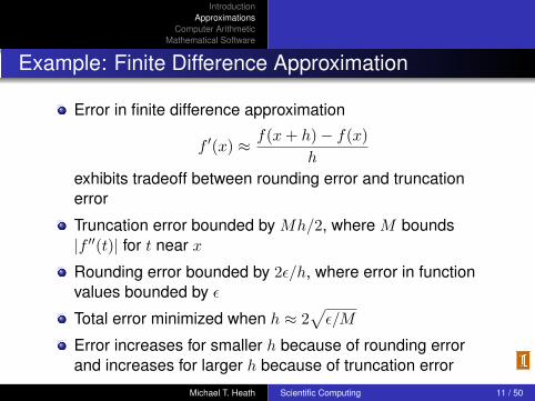
Error in finite difference approximation

f ′(x) ≈ f(x + h)− f(x)h

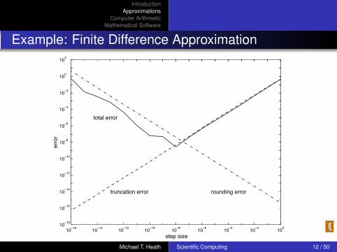
exhibits tradeoff between rounding error and truncationerror

Truncation error bounded by Mh/2, where M bounds|f ′′(t)| for t near x

Rounding error bounded by 2ε/h, where error in functionvalues bounded by ε

Total error minimized when h ≈ 2√

ε/M

Error increases for smaller h because of rounding errorand increases for larger h because of truncation error




Example: Finite Difference Approximation

!"!!#

!"!!$

!"!!%

!"!!"

!"!&

!"!#

!"!$

!"!%

!""

!"!!&

!"!!#

!"!!$

!"!!%

!"!!"

!"!&

!"!#

!"!$

!"!%

!""

!"%

'()*+',-)

)../.

(.0123(,/1+)../. ./014,15+)../.

(/(36+)../.




Forward and Backward Error

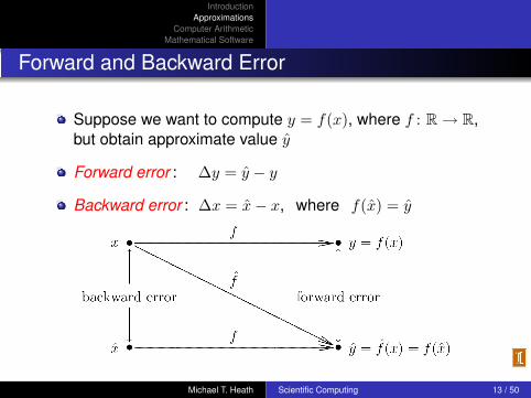
Suppose we want to compute y = f(x), where f : R → R,but obtain approximate value y

Forward error : ∆y = y − y

Backward error : ∆x = x− x, where f(x) = y




Example: Forward and Backward Error

As approximation to y =√

2, y = 1.4 has absolute forwarderror

|∆y| = |y − y| = |1.4− 1.41421 . . . | ≈ 0.0142

or relative forward error of about 1 percent

Since√

1.96 = 1.4, absolute backward error is

|∆x| = |x− x| = |1.96− 2| = 0.04

or relative backward error of 2 percent




Backward Error Analysis

Idea: approximate solution is exact solution to modifiedproblem

How much must original problem change to give resultactually obtained?

How much data error in input would explain all error incomputed result?

Approximate solution is good if it is exact solution to nearbyproblem

Backward error is often easier to estimate than forwarderror




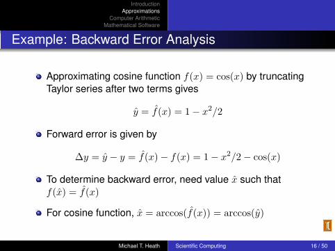
Example: Backward Error Analysis

Approximating cosine function f(x) = cos(x) by truncatingTaylor series after two terms gives

y = f(x) = 1− x2/2

Forward error is given by

∆y = y − y = f(x)− f(x) = 1− x2/2− cos(x)

To determine backward error, need value x such thatf(x) = f(x)

For cosine function, x = arccos(f(x)) = arccos(y)




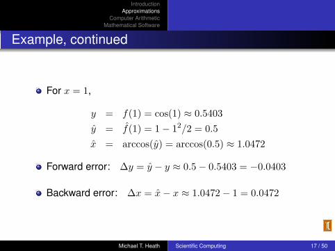
Example, continued

For x = 1,

y = f(1) = cos(1) ≈ 0.5403y = f(1) = 1− 12/2 = 0.5x = arccos(y) = arccos(0.5) ≈ 1.0472

Forward error: ∆y = y − y ≈ 0.5− 0.5403 = −0.0403

Backward error: ∆x = x− x ≈ 1.0472− 1 = 0.0472




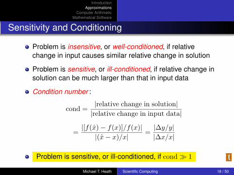
Sensitivity and Conditioning

Problem is insensitive, or well-conditioned, if relativechange in input causes similar relative change in solution

Problem is sensitive, or ill-conditioned, if relative change insolution can be much larger than that in input data

Condition number :

cond =|relative change in solution||relative change in input data|

=|[f(x)− f(x)]/f(x)|

|(x− x)/x|=|∆y/y||∆x/x|

Problem is sensitive, or ill-conditioned, if cond � 1




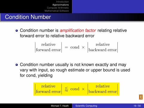
Condition Number

Condition number is amplification factor relating relativeforward error to relative backward error∣∣∣∣ relative

forward error

∣∣∣∣ = cond ×∣∣∣∣ relativebackward error

∣∣∣∣Condition number usually is not known exactly and mayvary with input, so rough estimate or upper bound is usedfor cond, yielding∣∣∣∣ relative

forward error

∣∣∣∣ / cond ×∣∣∣∣ relativebackward error

∣∣∣∣Michael T. Heath Scientific Computing 19 / 50



Example: Evaluating Function

Evaluating function f for approximate input x = x + ∆xinstead of true input x gives

Absolute forward error: f(x + ∆x)− f(x) ≈ f ′(x)∆x

Relative forward error:f(x + ∆x)− f(x)

f(x)≈ f ′(x)∆x

f(x)

Condition number: cond ≈∣∣∣∣f ′(x)∆x/f(x)

∆x/x

∣∣∣∣ = ∣∣∣∣xf ′(x)f(x)

∣∣∣∣Relative error in function value can be much larger orsmaller than that in input, depending on particular f and x




Example: Sensitivity

Tangent function is sensitive for arguments near π/2tan(1.57079) ≈ 1.58058× 105

tan(1.57078) ≈ 6.12490× 104

Relative change in output is quarter million times greaterthan relative change in input

For x = 1.57079, cond ≈ 2.48275× 105




Stability

Algorithm is stable if result produced is relativelyinsensitive to perturbations during computation

Stability of algorithms is analogous to conditioning ofproblems

From point of view of backward error analysis, algorithm isstable if result produced is exact solution to nearbyproblem

For stable algorithm, effect of computational error is noworse than effect of small data error in input




Accuracy

Accuracy : closeness of computed solution to true solutionof problem

Stability alone does not guarantee accurate results

Accuracy depends on conditioning of problem as well asstability of algorithm

Inaccuracy can result from applying stable algorithm toill-conditioned problem or unstable algorithm towell-conditioned problem

Applying stable algorithm to well-conditioned problemyields accurate solution




Floating-Point Numbers

Floating-point number system is characterized by fourintegers

β base or radixp precision[L,U ] exponent range

Number x is represented as

x = ±(

d0 +d1

β+

d2

β2+ · · ·+ dp−1

βp−1

)βE

where 0 ≤ di ≤ β − 1, i = 0, . . . , p− 1, and L ≤ E ≤ U




Floating-Point Numbers, continued

Portions of floating-poing number designated as follows

exponent : E

mantissa : d0d1 · · · dp−1

fraction : d1d2 · · · dp−1

Sign, exponent, and mantissa are stored in separatefixed-width fields of each floating-point word




Typical Floating-Point Systems

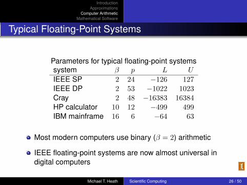
Parameters for typical floating-point systemssystem β p L U

IEEE SP 2 24 −126 127IEEE DP 2 53 −1022 1023Cray 2 48 −16383 16384HP calculator 10 12 −499 499IBM mainframe 16 6 −64 63

Most modern computers use binary (β = 2) arithmetic

IEEE floating-point systems are now almost universal indigital computers




Normalization

Floating-point system is normalized if leading digit d0 isalways nonzero unless number represented is zero

In normalized systems, mantissa m of nonzerofloating-point number always satisfies 1 ≤ m < β

Reasons for normalizationrepresentation of each number uniqueno digits wasted on leading zerosleading bit need not be stored (in binary system)




Properties of Floating-Point Systems

Floating-point number system is finite and discrete

Total number of normalized floating-point numbers is

2(β − 1)βp−1(U − L + 1) + 1

Smallest positive normalized number: UFL = βL

Largest floating-point number: OFL = βU+1(1− β−p)

Floating-point numbers equally spaced only betweensuccessive powers of β

Not all real numbers exactly representable; those that areare called machine numbers




Example: Floating-Point System

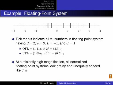
Tick marks indicate all 25 numbers in floating-point systemhaving β = 2, p = 3, L = −1, and U = 1

OFL = (1.11)2 × 21 = (3.5)10UFL = (1.00)2 × 2−1 = (0.5)10

At sufficiently high magnification, all normalizedfloating-point systems look grainy and unequally spacedlike this




Rounding Rules

If real number x is not exactly representable, then it isapproximated by “nearby” floating-point number fl(x)

This process is called rounding, and error introduced iscalled rounding error

Two commonly used rounding ruleschop : truncate base-β expansion of x after (p− 1)st digit;also called round toward zeroround to nearest : fl(x) is nearest floating-point number tox, using floating-point number whose last stored digit iseven in case of tie; also called round to even

Round to nearest is most accurate, and is default roundingrule in IEEE systems




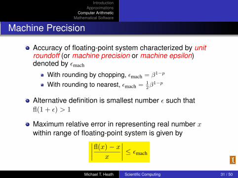
Machine Precision

Accuracy of floating-point system characterized by unitroundoff (or machine precision or machine epsilon)denoted by εmach

With rounding by chopping, εmach = β1−p

With rounding to nearest, εmach = 12β1−p

Alternative definition is smallest number ε such thatfl(1 + ε) > 1

Maximum relative error in representing real number xwithin range of floating-point system is given by∣∣∣∣fl(x)− x

x

∣∣∣∣ ≤ εmach




Machine Precision, continued

For toy system illustrated earlier

εmach = (0.01)2 = (0.25)10 with rounding by choppingεmach = (0.001)2 = (0.125)10 with rounding to nearest

For IEEE floating-point systems

εmach = 2−24 ≈ 10−7 in single precisionεmach = 2−53 ≈ 10−16 in double precision

So IEEE single and double precision systems have about 7and 16 decimal digits of precision, respectively




Machine Precision, continued

Though both are “small,” unit roundoff εmach should not beconfused with underflow level UFL

Unit roundoff εmach is determined by number of digits inmantissa of floating-point system, whereas underflow levelUFL is determined by number of digits in exponent field

In all practical floating-point systems,

0 < UFL < εmach < OFL




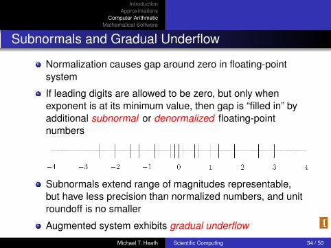
Subnormals and Gradual Underflow

Normalization causes gap around zero in floating-pointsystem

If leading digits are allowed to be zero, but only whenexponent is at its minimum value, then gap is “filled in” byadditional subnormal or denormalized floating-pointnumbers

Subnormals extend range of magnitudes representable,but have less precision than normalized numbers, and unitroundoff is no smaller

Augmented system exhibits gradual underflow




Exceptional Values

IEEE floating-point standard provides special values toindicate two exceptional situations

Inf, which stands for “infinity,” results from dividing a finitenumber by zero, such as 1/0NaN, which stands for “not a number,” results fromundefined or indeterminate operations such as 0/0, 0 ∗ Inf,or Inf/Inf

Inf and NaN are implemented in IEEE arithmetic throughspecial reserved values of exponent field




Floating-Point Arithmetic

Addition or subtraction : Shifting of mantissa to makeexponents match may cause loss of some digits of smallernumber, possibly all of them

Multiplication : Product of two p-digit mantissas contains upto 2p digits, so result may not be representable

Division : Quotient of two p-digit mantissas may containmore than p digits, such as nonterminating binaryexpansion of 1/10

Result of floating-point arithmetic operation may differ fromresult of corresponding real arithmetic operation on sameoperands




Example: Floating-Point Arithmetic

Assume β = 10, p = 6

Let x = 1.92403× 102, y = 6.35782× 10−1

Floating-point addition gives x + y = 1.93039× 102,assuming rounding to nearest

Last two digits of y do not affect result, and with evensmaller exponent, y could have had no effect on result

Floating-point multiplication gives x ∗ y = 1.22326× 102,which discards half of digits of true product




Floating-Point Arithmetic, continued

Real result may also fail to be representable because itsexponent is beyond available range

Overflow is usually more serious than underflow becausethere is no good approximation to arbitrarily largemagnitudes in floating-point system, whereas zero is oftenreasonable approximation for arbitrarily small magnitudes

On many computer systems overflow is fatal, but anunderflow may be silently set to zero




Example: Summing Series

Infinite series∞∑

n=1

1n

has finite sum in floating-point arithmetic even though realseries is divergent

Possible explanationsPartial sum eventually overflows1/n eventually underflowsPartial sum ceases to change once 1/n becomes negligiblerelative to partial sum

1/n < εmach

n−1∑k=1

(1/k)




Floating-Point Arithmetic, continued

Ideally, x flop y = fl(x op y), i.e., floating-point arithmeticoperations produce correctly rounded results

Computers satisfying IEEE floating-point standard achievethis ideal as long as x op y is within range of floating-pointsystem

But some familiar laws of real arithmetic are notnecessarily valid in floating-point system

Floating-point addition and multiplication are commutativebut not associative

Example: if ε is positive floating-point number slightlysmaller than εmach, then (1 + ε) + ε = 1, but 1 + (ε + ε) > 1




Cancellation

Subtraction between two p-digit numbers having same signand similar magnitudes yields result with fewer than pdigits, so it is usually exactly representable

Reason is that leading digits of two numbers cancel (i.e.,their difference is zero)

For example,

1.92403× 102 − 1.92275× 102 = 1.28000× 10−1

which is correct, and exactly representable, but has onlythree significant digits




Cancellation, continued

Despite exactness of result, cancellation often impliesserious loss of information

Operands are often uncertain due to rounding or otherprevious errors, so relative uncertainty in difference may belarge

Example: if ε is positive floating-point number slightlysmaller than εmach, then (1 + ε)− (1− ε) = 1− 1 = 0 infloating-point arithmetic, which is correct for actualoperands of final subtraction, but true result of overallcomputation, 2ε, has been completely lost

Subtraction itself is not at fault: it merely signals loss ofinformation that had already occurred




Cancellation, continued

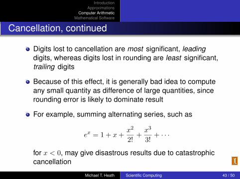
Digits lost to cancellation are most significant, leadingdigits, whereas digits lost in rounding are least significant,trailing digits

Because of this effect, it is generally bad idea to computeany small quantity as difference of large quantities, sincerounding error is likely to dominate result

For example, summing alternating series, such as

ex = 1 + x +x2

2!+

x3

3!+ · · ·

for x < 0, may give disastrous results due to catastrophiccancellation




Example: Cancellation

Total energy of helium atom is sum of kinetic and potentialenergies, which are computed separately and have oppositesigns, so suffer cancellation

Year Kinetic Potential Total1971 13.0 −14.0 −1.01977 12.76 −14.02 −1.261980 12.22 −14.35 −2.131985 12.28 −14.65 −2.371988 12.40 −14.84 −2.44

Although computed values for kinetic and potential energieschanged by only 6% or less, resulting estimate for total energychanged by 144%




Example: Quadratic Formula

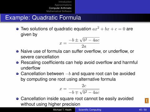
Two solutions of quadratic equation ax2 + bx + c = 0 aregiven by

x =−b±

√b2 − 4ac

2aNaive use of formula can suffer overflow, or underflow, orsevere cancellationRescaling coefficients can help avoid overflow and harmfulunderflowCancellation between −b and square root can be avoidedby computing one root using alternative formula

x =2c

−b∓√

b2 − 4ac

Cancellation inside square root cannot be easily avoidedwithout using higher precision




Example: Standard Deviation

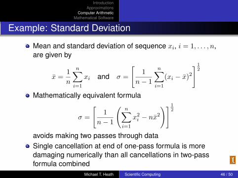
Mean and standard deviation of sequence xi, i = 1, . . . , n,are given by

x =1n

n∑i=1

xi and σ =

[1

n− 1

n∑i=1

(xi − x)2] 1

2

Mathematically equivalent formula

σ =

[1

n− 1

(n∑

i=1

x2i − nx2

)] 12

avoids making two passes through dataSingle cancellation at end of one-pass formula is moredamaging numerically than all cancellations in two-passformula combined




Mathematical Software

High-quality mathematical software is available for solvingmost commonly occurring problems in scientific computing

Use of sophisticated, professionally written software hasmany advantages

We will seek to understand basic ideas of methods onwhich such software is based, so that we can use softwareintelligently

We will gain hands-on experience in using such softwareto solve wide variety of computational problems




Desirable Qualities of Mathematical Software

ReliabilityRobustnessAccuracyEfficiencyMaintainabilityPortabilityUsabilityApplicability




Sources of Mathematical Software

FMM: From book by Forsythe/Malcolm/MolerGSL: GNU Scientific LibraryHSL: Harwell Subroutine LibraryIMSL: Internat. Math. & Stat. LibrariesKMN: From book by Kahaner/Moler/NashNAG: Numerical Algorithms GroupNetlib: Free software available via InternetNR: From book Numerical RecipesNUMAL: From Math. Centrum, AmsterdamSLATEC: From U.S. Government labsSOL: Systems Optimization Lab, Stanford U.TOMS: ACM Trans. on Math. Software




Scientific Computing Environments

Interactive environments for scientific computing provide

powerful mathematical capabilitiessophisticated graphics built-inhigh-level programming language for rapid prototyping

MATLAB is popular example, available for most personalcomputers and workstations

Similar, “free” alternatives include octave and Scilab

Symbolic computing environments, such as Maple andMathematica, are also useful


scientiﬁc computing: an introductory...

Documents