scienti c computing - math.tu-berlin.de · lecture on scienti c computing dr. kersten schmidt...

Lecture on

Scientific Computing

Dr. Kersten Schmidt

Lecture 4

Technische Universitat BerlinInstitut fur Mathematik

Wintersemester 2014/2015

Syllabus

I Linear Regression, Fast Fourier transformI Modelling by partial differential equations (PDEs)

I Maxwell, Helmholtz, Poisson, Linear elasticity, Navier-Stokes equationI boundary value problem, eigenvalue problemI boundary conditions (Dirichlet, Neumann, Robin)I handling of infinite domains (wave-guide, homogeneous exterior: DtN, PML)I boundary integral equations

I Computer aided-design (CAD)

I Mesh generatorsI Space discretisation of PDEs

I Finite difference methodI Finite element methodI Discontinuous Galerkin finite element method

I SolversI Linear Solvers (direct, iterative), preconditionerI Nonlinear Solvers (Newton-Raphson iteration)I Eigenvalue Solvers

I ParallelisationI SIMP: OpenMPI MIMP: MPI

,

VL Scientific Computing WS 2014/2015, Dr. K. Schmidt, 10/23/2014 2

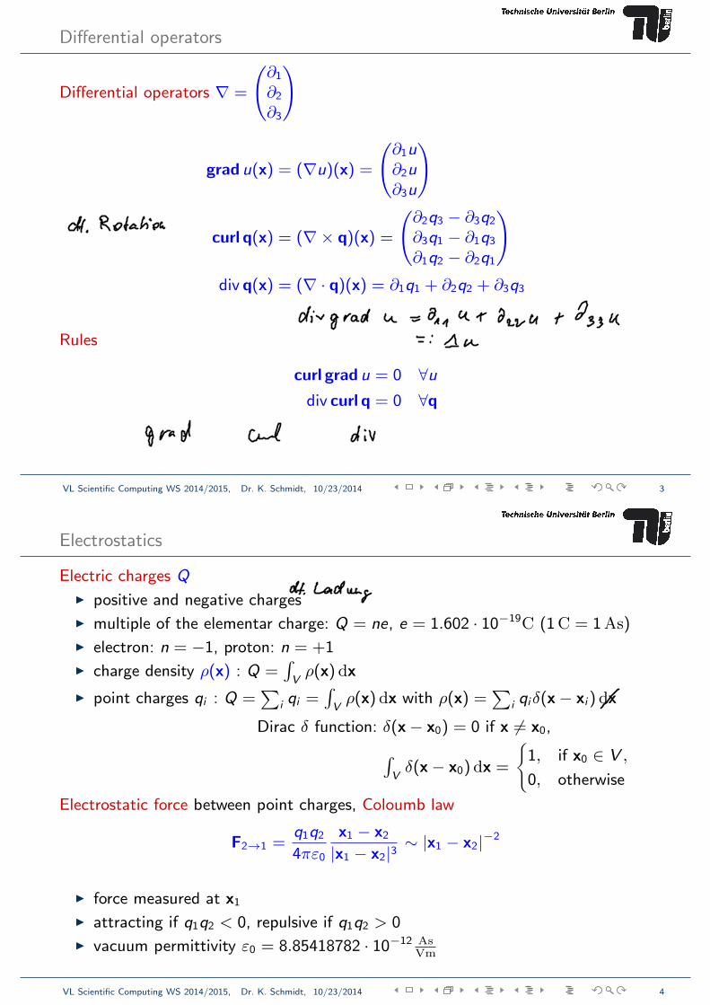
Differential operators

Differential operators ∇ =

(∂1

∂2

∂3

)

grad u(x) = (∇u)(x) =

(∂1u∂2u∂3u

)

curl q(x) = (∇× q)(x) =

(∂2q3 − ∂3q2

∂3q1 − ∂1q3

∂1q2 − ∂2q1

)

div q(x) = (∇ · q)(x) = ∂1q1 + ∂2q2 + ∂3q3

Rules

curl grad u = 0 ∀udiv curl q = 0 ∀q

,


Electrostatics

Electric charges Q

I positive and negative charges

I multiple of the elementar charge: Q = ne, e = 1.602 · 10−19C (1C = 1As)

I electron: n = −1, proton: n = +1

I charge density ρ(x) : Q =∫Vρ(x) dx

I point charges qi : Q =∑

i qi =∫Vρ(x) dx with ρ(x) =

∑i qiδ(x− xi ) dx

Dirac δ function: δ(x− x0) = 0 if x 6= x0,

∫Vδ(x− x0) dx =

®1, if x0 ∈ V ,

0, otherwise

Electrostatic force between point charges, Coloumb law

F2→1 =q1q2

4πε0

x1 − x2

|x1 − x2|3∼ |x1 − x2|−2

I force measured at x1

I attracting if q1q2 < 0, repulsive if q1q2 > 0

I vacuum permittivity ε0 = 8.85418782 · 10−12 AsVm

,


Electrostatics

Electrostatic force between point charges, Coloumb law

F2→1 =q1q2

4πε0

x1 − x2

|x1 − x2|3∼ |x1 − x2|−2

I force measured at x1

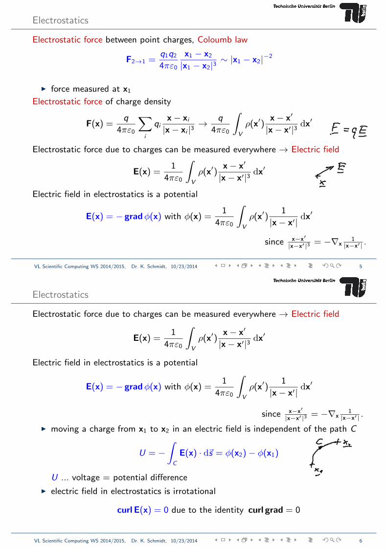
Electrostatic force of charge density

F(x) =q

4πε0

∑

i

qix− xi|x− xi |3

→ q

4πε0

∫

V

ρ(x′)x− x′

|x− x′|3 dx′

Electrostatic force due to charges can be measured everywhere → Electric field

E(x) =1

4πε0

∫

V

ρ(x′)x− x′

|x− x′|3 dx′

Electric field in electrostatics is a potential

E(x) = − gradφ(x) with φ(x) =1

4πε0

∫

V

ρ(x′)1

|x− x′| dx′

since x−x′|x−x′|3 = −∇x

1|x−x′| .

,


Electrostatics

Electrostatic force due to charges can be measured everywhere → Electric field

E(x) =1

4πε0

∫

V

ρ(x′)x− x′

|x− x′|3 dx′

Electric field in electrostatics is a potential

E(x) = − gradφ(x) with φ(x) =1

4πε0

∫

V

ρ(x′)1

|x− x′| dx′

since x−x′|x−x′|3 = −∇x

1|x−x′| .

I moving a charge from x1 to x2 in an electric field is independent of the path C

U = −∫

C

E(x) · d~s = φ(x2)− φ(x1)

U ... voltage = potential difference

I electric field in electrostatics is irrotational

curl E(x) = 0 due to the identity curl grad = 0

,


Electrostatics

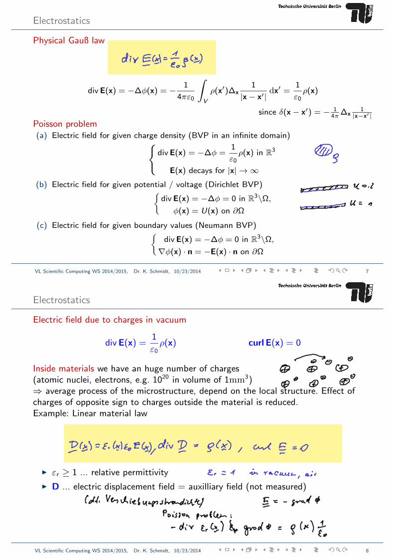
Physical Gauß law

div E(x) = −∆φ(x) = − 1

4πε0

∫

V

ρ(x′)∆x1

|x− x′| dx′ =

1

ε0ρ(x)

since δ(x− x′) = − 14π

∆x1

|x−x′|Poisson problem(a) Electric field for given charge density (BVP in an infinite domain)

div E(x) = −∆φ =1

ε0ρ(x) in R3

E(x) decays for |x| → ∞(b) Electric field for given potential / voltage (Dirichlet BVP)ß

div E(x) = −∆φ = 0 in R3\Ω,φ(x) = U(x) on ∂Ω

(c) Electric field for given boundary values (Neumann BVP)ßdiv E(x) = −∆φ = 0 in R3\Ω,∇φ(x) · n = −E(x) · n on ∂Ω

,


Electrostatics

Electric field due to charges in vacuum

divE(x) =1

ε0ρ(x) curl E(x) = 0

Inside materials we have an huge number of charges(atomic nuclei, electrons, e.g. 1020 in volume of 1mm3)⇒ average process of the microstructure, depend on the local structure. Effect ofcharges of opposite sign to charges outside the material is reduced.Example: Linear material law

I εr ≥ 1 ... relative permittivity

I D ... electric displacement field = auxilliary field (not measured)

,


Magnetostatics

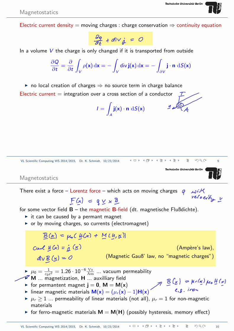
Electric current density = moving charges : charge conservation⇒ continuity equation

In a volume V the charge is only changed if it is transported from outside

∂Q

∂t=

∂

∂t

∫

V

ρ(x) dx = −∫

V

div j(x) dx = −∫

∂V

j · n dS(x)

I no local creation of charges ⇒ no source term in charge balance

Electric current = integration over a cross section of a conductor

I =

∫

A

j(x) · n dS(x)

,


Magnetostatics

There exist a force – Lorentz force – which acts on moving charges

for some vector field B – the magnetic B-field (dt. magnetische Flußdichte).I it can be caused by a permant magnetI or by moving charges, so currents (electromagnet)

(Ampere’s law),

(Magnetic Gauß’ law, no “magnetic charges”)

I µ0 = 1ε0c2 = 1.26 · 10−6 Vs

Am... vacuum permeability

I M ... magnetization, H ... auxilliary fieldI for permantent magnet j = 0, M = M(x)I linear magnetic materials M(x) = (µr (x)− 1)H(x)I µr ≥ 1 ... permeability of linear materials (not all), µr = 1 for non-magnetic

materialsI for ferro-magnetic materials M = M(H) (possibly hysteresis, memory effect)

,


Magnetostatics

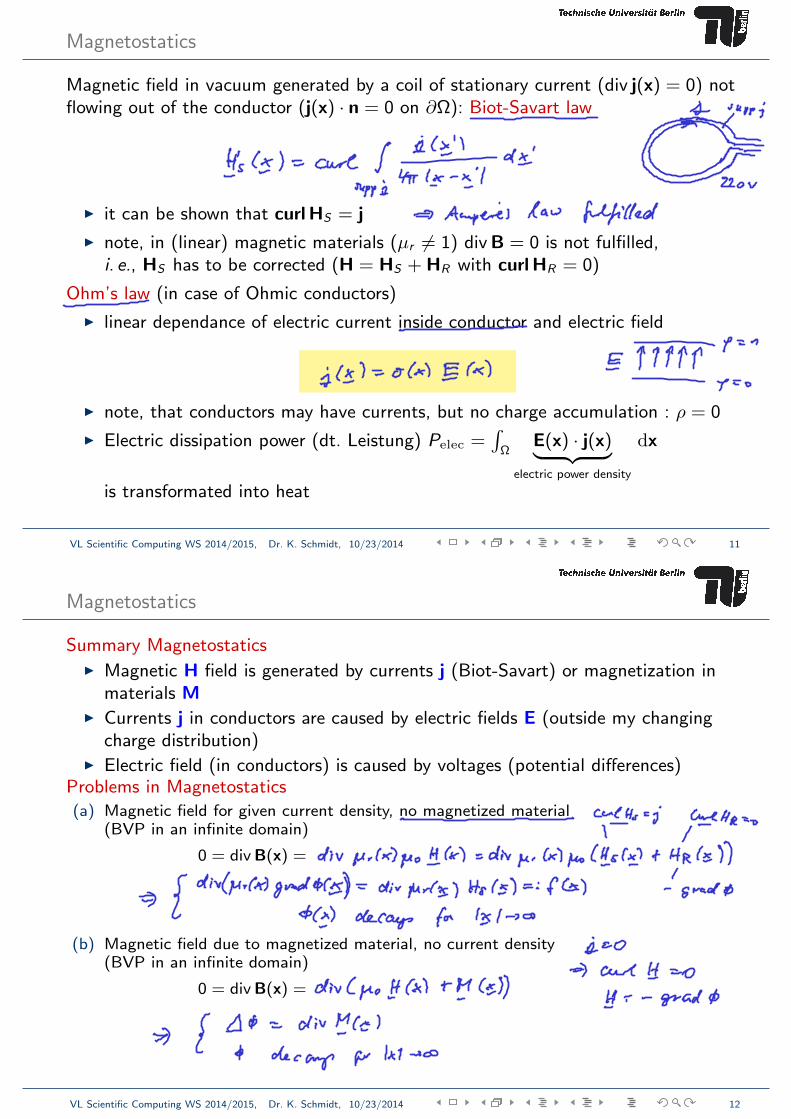
Magnetic field in vacuum generated by a coil of stationary current (div j(x) = 0) notflowing out of the conductor (j(x) · n = 0 on ∂Ω): Biot-Savart law

I it can be shown that curlHS = j

I note, in (linear) magnetic materials (µr 6= 1) divB = 0 is not fulfilled,i. e., HS has to be corrected (H = HS + HR with curlHR = 0)

Ohm’s law (in case of Ohmic conductors)

I linear dependance of electric current inside conductor and electric field

I note, that conductors may have currents, but no charge accumulation : ρ = 0

I Electric dissipation power (dt. Leistung) Pelec =∫

ΩE(x) · j(x)︸︷︷︸

electric power density

dx

is transformated into heat

,


Magnetostatics

Summary MagnetostaticsI Magnetic H field is generated by currents j (Biot-Savart) or magnetization in

materials MI Currents j in conductors are caused by electric fields E (outside my changing

charge distribution)I Electric field (in conductors) is caused by voltages (potential differences)

Problems in Magnetostatics

(a) Magnetic field for given current density, no magnetized material(BVP in an infinite domain)

0 = div B(x) =

(b) Magnetic field due to magnetized material, no current density(BVP in an infinite domain)

0 = div B(x) =

,


scienti c computing - math.tu-berlin.de · lecture on scienti c computing dr. kersten schmidt...

Documents