scidb user's guide - national energy research … user's guide iv 5.4. parallel load ........
TRANSCRIPT

SciDB User's Guide

SciDB User's GuideVersion 12.3Copyright © 2008–2012 SciDB, Inc.
SciDB is free software: you can redistribute it and/or modify it under the terms of the GNU General Public License, version 3, as published bythe Free Software Foundation.
SciDB is distributed "AS-IS" AND WITHOUT ANY WARRANTY OF ANY KIND, INCLUDING ANY IMPLIED WARRANTY OFMERCHANTABILITY, NON-INFRINGEMENT, OR FITNESS FOR A PARTICULAR PURPOSE. See the GNU General Public License at http://www.gnu.org/licenses/ for the complete license terms.

iii
Table of Contents1. Introduction to SciDB .................................................................................................... 1
1.1. Array Data Model ................................................................................................ 11.2. Basic Architecture ................................................................................................ 2
1.2.1. Chunking and Scalability ............................................................................. 21.2.2. Chunk Overlap .......................................................................................... 3
1.3. SciDB Array Storage ............................................................................................ 41.3.1. Instance Storage ........................................................................................ 41.3.2. SciDB System Catalog ................................................................................ 51.3.3. Transaction Model ..................................................................................... 5
1.4. Array Processing .................................................................................................. 51.4.1. Array Language ......................................................................................... 51.4.2. Query Building Blocks ............................................................................... 61.4.3. Pipelined Array Processing .......................................................................... 6
1.5. Clients and Connectors .......................................................................................... 61.6. Conventions Used in this Document ........................................................................ 7
2. SciDB Installation and Administration ................................................................................ 82.1. Installing SciDB ................................................................................................... 8
2.1.1. Preparing the Platform ................................................................................ 82.1.2. Install SciDB from binary package .............................................................. 11
2.2. Configuring SciDB ............................................................................................. 132.2.1. SciDB Configuration File .......................................................................... 132.2.2. Cluster Configuration Example ................................................................... 132.2.3. Logging Configuration .............................................................................. 15
2.3. Initializing and Starting SciDB .............................................................................. 162.3.1. The scidb.py Script ................................................................................... 16
2.4. Upgrading SciDB ............................................................................................... 172.4.1. Ubuntu ................................................................................................... 172.4.2. Red Hat and Fedora .................................................................................. 172.4.3. Additional Steps ....................................................................................... 18
3. Getting Started with SciDB Development .......................................................................... 193.1. Using the iquery Client ........................................................................................ 193.2. iquery Configuration ........................................................................................... 213.3. Example iquery session ........................................................................................ 21
4. Creating and Removing SciDB Arrays .............................................................................. 254.1. Create an Array .................................................................................................. 254.2. Array Attributes ................................................................................................. 27
4.2.1. NULL and Default Attribute Values ............................................................ 274.2.2. Codes for Missing Data ............................................................................. 28
4.3. Array Dimensions ............................................................................................... 284.3.1. Chunk Overlap ........................................................................................ 294.3.2. Unbounded Dimensions ............................................................................. 294.3.3. Noninteger Dimensions and Mapping Arrays ................................................. 29
4.4. Changing Array Names ........................................................................................ 304.5. Database Design ................................................................................................. 30
4.5.1. Selecting Dimensions and Attributes ............................................................ 304.5.2. Chunk Size Selection ................................................................................ 31
5. Loading Data ................................................................................................................ 325.1. Simple Data Loading ........................................................................................... 325.2. Data with Special Values ..................................................................................... 345.3. Sparse Load Format ............................................................................................ 34
5.3.1. Sparse Load Chunks ................................................................................. 35

SciDB User's Guide
iv
5.4. Parallel Load ..................................................................................................... 365.5. Saving Data from a SciDB Array to a File .............................................................. 36
6. Basic Array Tasks ......................................................................................................... 386.1. Selecting Data From an Array ............................................................................... 38
6.1.1. The SELECT Statement ............................................................................ 386.2. Array Joins ........................................................................................................ 396.3. Aliases .............................................................................................................. 416.4. Nested Subqueries .............................................................................................. 416.5. Data Sampling ................................................................................................... 41
7. Aggregates ................................................................................................................... 437.1. Grand Aggregates ............................................................................................... 447.2. Group-By Aggregates .......................................................................................... 457.3. Grid Aggregates ................................................................................................. 467.4. Window Aggregates ............................................................................................ 47
8. Updating Your Data ...................................................................................................... 498.1. The UPDATE ... SET statement ............................................................................ 498.2. Array Versions ................................................................................................... 49
9. Changing Array Schemas: Transforming Your SciDB Array ................................................. 519.1. Redimensioning an Array ..................................................................................... 51
9.1.1. Redimensioning Arrays Containing Null Values ............................................. 529.2. Array Transformations ......................................................................................... 53
9.2.1. Rearranging Array Data ............................................................................. 549.2.2. Reduce an Array ...................................................................................... 55
9.3. Changing Array Attributes .................................................................................... 579.4. Changing Array Dimensions ................................................................................. 58
9.4.1. Changing Chunk Size ............................................................................... 589.4.2. Appending a Dimension ............................................................................ 59
10. SciDB Aggregate Reference .......................................................................................... 61avg ......................................................................................................................... 62count ...................................................................................................................... 63max ........................................................................................................................ 64min ......................................................................................................................... 65stdev ....................................................................................................................... 66sum ........................................................................................................................ 67var ......................................................................................................................... 68
11. SciDB Function Reference ............................................................................................ 6912. SciDB Data Type Reference .......................................................................................... 7113. SciDB Operator Reference ............................................................................................ 72
adddim .................................................................................................................... 73analyze .................................................................................................................... 74apply ...................................................................................................................... 76attribute_rename ....................................................................................................... 77attributes ................................................................................................................. 78avg ......................................................................................................................... 79bernoulli .................................................................................................................. 80between ................................................................................................................... 82build ....................................................................................................................... 83build_sparse ............................................................................................................. 84cancel ..................................................................................................................... 85cast ......................................................................................................................... 86concat ..................................................................................................................... 87count ...................................................................................................................... 88cross ....................................................................................................................... 90cross_join ................................................................................................................ 91
SciDB User's Guide
v
deldim .................................................................................................................... 93dimensions ............................................................................................................... 94diskinfo ................................................................................................................... 95echo ....................................................................................................................... 96explain_logical ......................................................................................................... 97filter ....................................................................................................................... 98help ........................................................................................................................ 99input ..................................................................................................................... 100inverse .................................................................................................................. 101join ....................................................................................................................... 102list ........................................................................................................................ 103load_library ............................................................................................................ 104lookup ................................................................................................................... 105max ...................................................................................................................... 107merge .................................................................................................................... 108min ....................................................................................................................... 109multiply ................................................................................................................. 110normalize ............................................................................................................... 111project ................................................................................................................... 112redimension ............................................................................................................ 113redimension_store .................................................................................................... 115reduce_distro .......................................................................................................... 117regrid .................................................................................................................... 118remove .................................................................................................................. 119rename .................................................................................................................. 120repart .................................................................................................................... 121reshape .................................................................................................................. 122reverse .................................................................................................................. 123sample ................................................................................................................... 124save ...................................................................................................................... 125scan ...................................................................................................................... 126setopt .................................................................................................................... 127show ..................................................................................................................... 128slice ...................................................................................................................... 129sort ....................................................................................................................... 130stdev ..................................................................................................................... 131store ...................................................................................................................... 132subarray ................................................................................................................. 133substitute ............................................................................................................... 134sum ...................................................................................................................... 135thin ....................................................................................................................... 136transpose ............................................................................................................... 138unload_library ......................................................................................................... 139unpack .................................................................................................................. 140var ........................................................................................................................ 142versions ................................................................................................................. 143window ................................................................................................................. 144xgrid ..................................................................................................................... 145

1
Chapter 1. Introduction to SciDBSciDB is an all-in-one data management and advanced analytics platform. It provides massively scalablecomplex analytics inside a next-generation database with data versioning to support the needs ofcommercial and scientific applications. SciDB is an open source software platform that runs on a grid ofcommodity hardware or in a cloud.
Paradigm4 Enterprise SciDB with Paradigm4 Extensions is an enterprise distribution of SciDB withadditional linear algebra operations, high availability options, and client connector features.
Unlike conventional relational databases designed around a row or column-oriented table data model,SciDB is an array database. The native array data model provides compact data storage and highperformance operations on ordered data such as spatial (location-based) data, temporal (time series) data,and matrix-based data for linear algebra operations.
This document is a User's Guide, written for scientists and developers in various application areas whowant to use SciDB as their scalable data management and analytic platform.
This chapter introduces the key technical concepts in SciDB—its array data model, basic systemarchitecture including distributed data management, salient features of the local storage manager, andthe system catalog. It also provides an introduction to SciDB's array languages—Array Query Language(AQL) and Array Functional Language (AFL)—and an overview of transactions in SciDB.
1.1. Array Data ModelSciDB uses multidimensional arrays as its basic storage and processing unit. A user creates a SciDB arrayby specifying dimensions and attributes of the array.
Dimensions
An n-dimensional SciDB array has dimensions d1, d2, ..., dn. The size of the dimension is the number ofordered values in that dimension. For example, a 2-dimensional array may have dimensions i and j, eachwith values (1, 2, 3, ..., 10) and (1, 2, ..., 30) respectively.
Basic array dimensions are 64-bit integers. SciDB also supports arrays with one or more nonintegerdimensions, such as variable-length strings (alpha, beta, gamma, ...) or floating-point values (1.2, 2.76,4.3, ...).
When the total number of values or cardinality of a dimension is known in advance, the SciDB array canbe declared with a bounded dimension. However, in many cases, the cardinality of the dimension maynot be known at array creation time. In such cases, the SciDB array can be declared with an unboundeddimension.
Attributes
Each combination of dimension values identifies a cell or element of the array, which can hold multipledata values called attributes (a1, a2, ..., am). Each data value is referred to as an attribute, and belongs toone of the supported datatypes in SciDB.
At array creation time, the user must specify:
• An array name.
• Array dimensions. The name and size of each dimension must be declared.

Introduction to SciDB
2
• Array attributes of the array. The name and data type of the each attribute must be declared.
Once you have created a SciDB database and defined the arrays, you must prepare and load data into it.Loaded data is then available to be accessed and queried using SciDB's built-in analytics capabilities.
1.2. Basic ArchitectureSciDB uses a shared-nothing architecture which is shown in the illustration below.
SciDB is deployed on a cluster of servers, each with processing, memory, and local storage, interconnectedusing a standard ethernet and TCP/IP network. Each physical server hosts a SciDB instance that isresponsible for local storage and processing.
External applications, when they connect to a SciDB database, connect to one of the instances in the cluster.While all instances in the SciDB cluster participate in query execution and data storage, one server is thecoordinator and orchestrates query execution and result fetching. It is the responsibility of the coordinatorinstance to mediate all communication between the SciDB external client and the entire SciDB database.The rest of the system instances are referred to as worker instances and work on behalf of the coordinatorfor query processing.
SciDB's scale-out architecture is ideally suited for hardware grids as well as clouds, where additionalsevers may be added to scale the total capacity.
1.2.1. Chunking and ScalabilityWhen data is loaded, it is partitioned and stored on each instance of the SciDB database. SciDB useschunking, a partitioning technique for multidimensional arrays where each instance is responsible forstoring and updating a subset of the array locally, and for executing queries that use the locally stored

Introduction to SciDB
3
data. By distributing data uniformly across all instances, SciDB is able to deliver scalable performance oncomputationally or I/O intensive analytic operations on very large data sets.
The details of chunking are shown in this section. Remember that you do not need to manage chunkdistribution beyond specifying chunk size.
Chunking is specified for each array as follows. Each dimension of an array is divided into chunks. Forexample, an array with dimensions i and j, where i is of length 10 and chunk size 5 and j is of length30 and chunk size 10 would be chunked as follows:
Chunks are arranged in row-major order in this example, and stored within the cluster using a round-robindistribution as follows. Suppose a cluster has instances 1 through 4, the placement of data is shown below.
C11 -> server 1
C12 -> server 2
C13 -> server 3
C21 -> server 4
C22 -> server 1
C23 -> server 2
This scheme is generalized to arrays with more dimensions by arranging the chunks in left-to-rightdimension order.
1.2.2. Chunk OverlapIt is sometimes advantageous to have neighboring chunks of an array overlap with each other. Overlap isspecified for each dimension of an array. For example, consider an array A as follows:
A<a: int32>[i=1:10,5,1, j=1:30,10,5]

Introduction to SciDB
4
Array A has has two dimensions, i and j. Dimension i is of length 10, chunk size 5, and had chunkoverlap 1. Dimension j has length 30, chunk size 10, and chunk overlap 5. This overlap causes SciDB tostore adjoining cells in each dimension from the overlap area in both chunks.
Some advantages of chunk overlap are:
• Speeding up nearest-neighbor queries, where each chunk may need access to a few elements from itsneighboring chunks,
• Detecting data clusters or data features that straddle more than one chunk.
SciDB supports operators that can be used to add or change the chunk overlap within an existing array.
1.3. SciDB Array StorageSciDB arrays consist of array chunk storage and array metadata stored in the system catalog. When arraysare created, updated, or removed, they are done using transactions. Transactions span array storage andthe system catalog and ensure consistency of the overall database as queries are executed.
The following sections describe SciDB's instance storage, system catalog, and transaction model.
1.3.1. Instance StorageVertical partitioning Each local SciDB instance divides logical chunks of an array into
per-attribute chunks, a technique referred to as vertical partitioning.All basic array processing steps—storage, query processing,and data transfer between instances—use single-attribute chunks.SciDB uses run-length encoding internally to compress repeatedvalues or commonly occurring patterns typical in scientificapplications. Frequently accessed chunks are maintained in an in-memory cache and accelerate query processing by eliminatingexpensive disk fetches for repeatedly accessed data.
Storage of array versions SciDB uses a "no overwrite" storage model. No overwrite meansthat data is never overwritten; each query that stores or updatesexisting arrays writes a new full chunk or a new delta chunk. Deltachunks are calculated by differencing the new version with the priorversion and only storing the difference. The SciDB storage managerstores "reverse" deltas—this means that the most recent version ismaintained as a full chunk, and prior versions are maintained asa list or chain of reverse deltas. The delta chain is stored in the"reserve" portion of each chunk, an additional area over and abovethe total size of the chunk. If the reserve area for the chunk fills up,a new chunk is allocated within the same segment or a new segmentand linked into the delta chain.
Storage segments The local storage manager manages space allocation, placement,and reclamation within the local storage manager using segments.A storage segment is a contiguous portion of the storage filereserved for successive chunks of the same array. This is designedto optimize queries issued on a very large array to use sequentialdisk I/O and hence maximize the rate of data transfer during a query.
Segments also serve as the unit of storage reclaim, so that as arraychunks are created, written, and ultimately removed, a segment

Introduction to SciDB
5
is reclaimed and reallocated for new chunks or arrays once allits member chunks have been removed. This allows for reuse ofstorage space.
Transient storage SciDB uses temporary data files or "scratch space" during queryexecution. This is specified during initialization and start-up as thetmp-path configuration setting. Temporary files are managedusing the operating system's tempfile mechanism. Data written totempfile only last for the lifetime of a query. They are removedupon successful completion or abort of the query.
1.3.2. SciDB System CatalogSciDB relies on a system catalog that is a repository of the following information:
• Configuration and status information about the SciDB cluster,
• Array-related metadata such as array definitions, array versions, and associations between arrays andother related objects,
• Information about SciDB extensions, such as plug-in libraries containing user-defined objects, whichare described in the section "Array Processing."
The system catalog in current versions of SciDB is implemented as PostgresSQL tables. The tables areshared between all SciDB instances within the cluster.
1.3.3. Transaction ModelSciDB combines traditional ACID semantics with versioned, no overwrite array storage. When usingversioned arrays, write transactions create new versions of the array—they do not modify pre-existingversions of the array.
The scope of a transaction in SciDB is a single statement. Each statement involves many operations onone or more arrays. Ultimately, the transaction stores the result into a destination array.
SciDB implements array-level locking. Locks are acquired at the beginning of a transaction and are used toprotect arrays during queries. Locks are released upon completion of the query. If a query aborts, pendingchanges are undone at all instances in the system catalog, and the database is returned to a prior consistentstate.
1.4. Array ProcessingSciDB's query languages provide the basic framework for scalable array processing.
1.4.1. Array LanguageSciDB provides two query language interfaces.
• AQL, the Array Query Language
• AFL, the Array Functional Language
SciDB's Array Query Language (AQL) is a high-level declarative language for working with SciDB arrays.It is similar to the SQL language for relational databases, but uses an array-based data model and a morecomprehensive analytical query set compared with standard relational databases.

Introduction to SciDB
6
AQL represents the full set of data management and analytic capabilities including data loading, dataselection and projection, aggregation, and joins.
The AQL language includes two classes of queries:
• Data Definition Language (DDL) : commands to define arrays and load data.
• Data Manipulation Language (DML) : commands to access and operate on array data.
AQL statements are handled by the SciDB query compiler which translates and optimizes incomingstatements into an execution plan.
SciDB's Array Functional Language (AFL) is a functional language for working with SciDB arrays. AFLoperators are used to compose queries or statements.
1.4.2. Query Building BlocksThere are four building blocks that you use to control and access your data. These building blocks are:
Operators SciDB operators, such as join, take one or more SciDB arrays asinput and return a SciDB array as output.
Functions SciDB functions, such as sqrt, take scalar values from literals orSciDB arrays and return a scalar value.
Data types Data types define the classes of values that SciDB can store andperform operations on.
Aggregates SciDB aggregates take an arbitrarily large set of values as input andreturn a scalar value.
Any of these building blocks can be user-defined, that is, users can write new operators, data types,functions, and aggregates.
1.4.3. Pipelined Array ProcessingWhen a SciDB query is issued, it is setup as a pipeline of operators. Operators are responsible for dataprocessing and aggregation as well as intermediate data exchange and data storage.
Execution begins when the client issues a request to fetch a chunk from the result array. Data is thenscanned from array storage on all instances and streamed into and out of each operator one chunk at a time.This model of query execution is sometimes referred to as pull-based execution and the operators that usethis model are called streaming operators. Unless required by the data processing algorithm, all SciDBoperators are streaming operators. Some operators implement algorithms that require the entire array tobe materialized in memory at all instances at once. These are referred to as materializing operators.
1.5. Clients and ConnectorsThe SciDB software package that you downloaded contains a special command line utility called iquerywhich provides an interactive Linux shell and supports both AQL and AFL. For more information aboutiquery, see Getting Started With SciDB Development.
Client applications connect to SciDB using an appropriate connector package which implements the client-side of the SciDB client-server protocol. Once connected via the connector, the user may issue querieswritten in either AFL or AQL, and fetch the result of a query using an iterator interface.

Introduction to SciDB
7
1.6. Conventions Used in this DocumentCode to be typed in verbatim is shown in fixed-width font. Code that is to be replaced with anactual string is shown in italics. Optional arguments are shown in square brackets [].
AQL commands are shown in FIXED-WIDTH BOLD CAPS. When necessary, a line of code may bepreceded by the AQL% or AFL% prompt to show which language the query is issued from.

8
Chapter 2. SciDB Installation andAdministration
2.1. Installing SciDBSciDB binaries are currently available for the following Linux platforms:
• Red Hat Enterprise Linux 5.4
• Fedora 11
• Ubuntu 11.04
For virtual machine–based installs, you can use VMWare Player or VBox for desktop testing and CitrixXenServer for production use.
The following terms are used to describe the SciDB installation and administration process:
Instance An independent SciDB process, that is, a single runnable copyof SciDB. There may be a many-to-one mapping between SciDBinstances and a single server.
Cluster A group of one or more single servers connected by TCP/IP,working together as a single system, and sharing data. A cluster canbe a private grid or a public cloud.
Single server A configuration that consists of a single machine with a processorthat may contain any number of cores, memory and attachedstorage. A single server may be virtual or physical. A single serveris not connected to nor does it share data with any other servers ina cluster.
Virtual server A server that shares hardware rather than having dedicatedhardware.
2.1.1. Preparing the Platform
2.1.1.1. Linux User Account
First, you will need to create a Linux user account, scidb. This account will be used to run all SciDBprocesses and own all files created by SciDB. The scidb user account must have superuser privileges. Itis also helpful to set up the account for access to the system without password entry.
To create the account, modify the /etc/sudoers file as follows:
## Allow root to run any commands anywhereroot ALL=(ALL) ALLscidb ALL=(ALL) NOPASSWD: ALL

SciDB Installation and Administration
9
2.1.1.2. Postgres Installation and Configuration
SciDB has been tested with Postgres 8.4.X. A suitable version of Postgres (8.4.6 or 8.4.7) is typicallyavailable on most Linux platforms.
On Ubuntu, you can use apt-get to install the postgresql-contrib package:
sudo apt-get install postgresql-contrib
On Red Hat and Fedora, you can use yum :
sudo yum install postgresql-contrib
By default, Postgres is configured to allow only local access via Unix-domain sockets. In a clusterenvironment, the Postgres database needs to be configured to allow access from other instances in thecluster. To do this:
1. Modify the pg_hba.conf file (usually at /etc/postgresql/8.4/main/ or /var/lib/pgsql/data/) by adding the following line:
host all all 10.0.0.1/8 trust
2. In the pg_hba.conf file, change all instances of 'ident' to 'trust' (assuming your local network is10.x.x.x).
3. Restart Postgres.
Warning
This Postgres configuration might pose security issues. When authentication is set to trustPostgreSQL assumes that anyone who can connect to the server is authorized to access thedatabase. To make a more secure installation, you can list specific host IP addresses, user names,and role mappings.
You can read more on the security details of Postgres client-authentication in the Postgresdocumentation at http://www.postgresql.org/docs/8.3/static/client-authentication.html.
You might need to set the postgresql.conf file to have it listen on the relevant port and IP address,as it might be limited to localhost by default.
If you are running a cluster with multiple servers, you will also need to modify the postgresql.conffile to allow connections:
# - Connection Settings -listen_addresses = '*'
You can verify that a PostgreSQL instance is running on the coordinator with the status command:
sudo /etc/init.d/postgresql-8.4 statussudo /etc/init.d/postgresql-8.4 start
Note
• Red Hat Enterprise Linux 5.4 comes with PostgreSQL 8.1. We recommend upgrading toversion 8.4.7.

SciDB Installation and Administration
10
• Add Postgres startup scripts to the Linux initialization scripts to start Postgres automaticallyafter a reboot.
• If your scidb user does not have sudo privileges, have your administrator use the followingprocedure to initialize Postgres:
1. Create a new role or account (say test1user) with password (say test1passwd).
2. Create a database for testing scidb (say test1) using the new account.
3. Create a schema in that newly created Postgres database to hold the SciDB catalog data:
root$ sudo -u postgres /opt/scidb/12.3/bin/scidb-prepare-db.sh
The last step, after you have configured Postgres, is to add it to Linux system services. This means thatPostgres will be started automatically on system reboot:
sudo /sbin/chkconfig --add postgresql
2.1.1.3. Remote Execution Configuration (ssh)
SciDB uses ssh for remote execution of cluster management commands. This is why the scidb useraccount should have no-password ssh access from the coordinator to the workers and from the coordinatorto itself.
The python-crypto (64-bit) and python-paramiko packages are required for SciDB on Red Hat5.4. These packages are ssh packages in Python. You can install the Python ssh client packages asfollows:
sudo apt-get install python, python-crypto, python-paramiko
There are several methods to configure no-password ssh between servers. We recommend the followingsimple method.
1. Create a key:
ssh-keygen
2. Copy the key to the localhost (or coordinator) and to each worker:
ssh-copy-id scidb@workerssh-copy-id scidb@localhost
3. Login to remote host. Note that no password is required now:
ssh scidb@worker
2.1.1.4. Shared file system
To run SciDB in a cluster , export the /opt/scidb directory on the coordinator using NFS or samba.To do this, configure the export and restart the NFS service like this:
# Configure the export
SciDB Installation and Administration
11
/opt/scidb *(ro,no_root_squash,sync)
# Restart the nfs servicesudo /etc/init.d/nfs restart
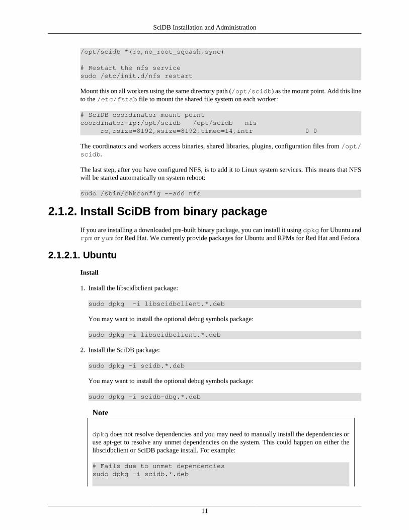
Mount this on all workers using the same directory path (/opt/scidb) as the mount point. Add this lineto the /etc/fstab file to mount the shared file system on each worker:
# SciDB coordinator mount pointcoordinator-ip:/opt/scidb /opt/scidb nfs ro,rsize=8192,wsize=8192,timeo=14,intr 0 0
The coordinators and workers access binaries, shared libraries, plugins, configuration files from /opt/scidb.
The last step, after you have configured NFS, is to add it to Linux system services. This means that NFSwill be started automatically on system reboot:
sudo /sbin/chkconfig --add nfs
2.1.2. Install SciDB from binary packageIf you are installing a downloaded pre-built binary package, you can install it using dpkg for Ubuntu andrpm or yum for Red Hat. We currently provide packages for Ubuntu and RPMs for Red Hat and Fedora.
2.1.2.1. Ubuntu
Install
1. Install the libscidbclient package:
sudo dpkg -i libscidbclient.*.deb
You may want to install the optional debug symbols package:
sudo dpkg -i libscidbclient.*.deb
2. Install the SciDB package:
sudo dpkg -i scidb.*.deb
You may want to install the optional debug symbols package:
sudo dpkg -i scidb-dbg.*.deb
Note
dpkg does not resolve dependencies and you may need to manually install the dependencies oruse apt-get to resolve any unmet dependencies on the system. This could happen on either thelibscidbclient or SciDB package install. For example:
# Fails due to unmet dependenciessudo dpkg -i scidb.*.deb

SciDB Installation and Administration
12
# Installs dependenciessudo apt-get -f install
# Succeeds nowsudo dpkg -i scidb-RelWithDebInfo-12.3.*.deb
Uninstall
Uninstall SciDB as follows:
sudo dpkg -r scidb-dbgsudo dpkg -r scidbsudo dpkg -r libscidbclient-dbgsudo dpkg -r libscidbclient
2.1.2.2. Red Hat and Fedora
Install:
1. Install the libscidbclient package:
sudo rpm --force -ivh libscidbclient-RelWithDebInfo-12.3.*.rpm
You may want to install the optional debug symbols package:
sudo rpm --force -ivh libscidbclient-dbg.*.rpm
2. Next, install the SciDB server package:
sudo rpm --force -ivh scidb-12.3.*.rpm
You may want to install the optional debug symbols package:
sudo rpm --force -ivh scidb-dbg.*.rpm
Uninstall:
To uninstall SciDB, do the following:
sudo rpm -e scidb-dbgsudo rpm -e scidbsudo rpm -e libscidbclient-dbgsudo rpm -e libscidbclient
2.1.2.3. Environment Variables
Now you need to configure the environment of the scidb user account. The following lines should beadded to the user's shell configuration file (often .profile or .bashrc ):
export SCIDB_VER=12.3export PATH=/opt/scidb/$SCIDB_VER/bin: /opt/scidb/$SCIDB_VER/share/scidb:$PATHexport LD_LIBRARY_PATH=/opt/scidb/$SCIDB_VER/lib:$LD_LIBRARY_PATH

SciDB Installation and Administration
13
2.2. Configuring SciDBThis chapter demonstrates how to configure SciDB prior to initialization, including checking that thePostgreSQL DBMS is running, that the SciDB configuration file (usually /opt/scidb/12.3/etc/config.ini) is set up, and that logging is configured.
2.2.1. SciDB Configuration FileYou need to create a configuration file for SciDB. It is named config.ini and it resides in the etcsub-directory of the installation tree. (By default it is /opt/scidb/12.3/etc/config.ini.) Theconfiguration file can have multiple sections, one per service instance.
The configuration 'test1' below is an example of the configuration for a single-instance system (coordinatoronly):
[test1]instance-0=localhost,0db_user=test1userdb_passwd=test1passwdinstall_root=/opt/scidb/12.3metadata=/opt/scidb/12.3/share/scidb/meta.sqlpluginsdir=/opt/scidb/12.3/lib/scidb/pluginslogconf=/opt/scidb/12.3/share/scidb/log4cxx.propertiesbase-path=/home/scidb/database-port=1239interface=eth0no-watchdog=trueredundancy=1merge-sort-buffer=1024network-buffer=1024mem-array-threshold=1024smgr-cache-size=1024execution-threads=16result-prefetch-queue-size=4result-prefetch-threads=4chunk-segment-size=10485760
2.2.2. Cluster Configuration ExampleThe following SciDB cluster configuration is called 'monolith'. This cluster consists of eight identicalvirtual servers:
• x86 6-core processor
• 8 GB of RAM
• 1 TB direct attached storage
• 1Gbps Ethernet
• RHEL 5.4
The following configuration file applies to such a cluster and is explained in the following section.

SciDB Installation and Administration
14
[monolith]# server-id=IP, number of worker instancesserver-0=10.0.20.231,0server-1=10.0.20.232,1server-2=10.0.20.233,1server-3=10.0.20.234,1server-4=10.0.20.235,1server-5=10.0.20.236,1server-6=10.0.20.237,1server-7=10.0.20.238,1db_user=monolithdb_password=monolithinstall_root=/opt/scidb/12.3metadata=/opt/scidb/12.3/share/scidb/meta.sqlpluginsdir=/opt/scidb/12.3/lib/scidb/pluginslogconf=/opt/scidb/log4cxx.properties.tracebase-path=/data/monolith_database-port=1239interface=eth0
The install package contains a sample configuration file, sample_config.ini, with examples.
The following table describes the basic configuration file settings:
Basic Configuration
Key Value
Cluster name Name of the SciDB cluster. The cluster name must appear as a section headingin the config.ini file, e.g., [cluster1]
server-N The host name or IP address used by server N and the number of workerinstances on it. Server 0 always has the coordinator running as instance 0, andmay have additional worker instances running as well.
db_user Username to use in the catalog connection string. This example uses test1user
db_passwd Password to use in the catalog connection string. This example usestest1passwd
install_root Path name of install root.
metadata Metadata definition file.
pluginsdir The folder or directory in which plugins are stored.
logconf log4xx configuration file.
The following table describes the cluster configuration file contents and how to set them:
Cluster Configuration
Key Value
base-path The root data directory for each SciDB instance. Each SciDB instanceinitializes its data directory within the base-path. Path scidb/00n/1 will bethe path for instance n.
base-port Base port number. Connections to the coordinator (and therefore to the system)are via this number, while worker instances communicate at base-port +instance number. The default number that iquery expects is 1239.

SciDB Installation and Administration
15
interface Ethernet interface that SciDB must use.
ssh-port (optional) The port that ssh uses for communications within the cluster. Default:22.
key-file-list (optional) Comma-separated list of filenames that include keys for ssh authentication.Default: None.
tmp-path (optional) The directory to use as temporary space.
no-watchdog (optional) Set this to true if you do not want automatic restart of the SciDB server on asoftware crash. Default: false.
The following table describes the configuration file elements for tuning your system performance:
Performance Configuration
Key Value
save-ram (optional) 'True', 'true', 'on' or 'On' will enable this option. Off by default. Thisallows you to store temporary data in memory. It is not advisable todo this; it is better to store temporary data in files.
merge-sort-buffer (optional) Size of memory buffer used in merge sort. Default: 512 MB.
mem-array-threshold (optional) Maximum memory used for temporary arrays. Default: 1024 MB.
chunk-reserve (optional) Percentage of chunk preallocated to store chunk deltas. Setting thisparameter to 0 disables the delta mechanism. Default: 10%.
chunk-segment-size (optional) Size in bytes of a storage segment. A storage segment is a unit ofallocation and reclamation used by storage manager. If set to zero, nospace reuse or storage reclamation is done.
execution-threads (optional) Size of thread pool available for query execution. Shared pool ofthreads used by all queries for network IO and some query executiontasks. Default: 4.
operator-threads (optional) Limit the number of threads allocated per (multithreaded) operatorin a query. If operator-threads is unspecified, SciDB automaticallydetects the number of CPU cores and uses that value. If you arerunning multiple instances on each server, operator-threads must beset lower than the number of CPU cores since multiple instances sharethe same set of CPU cores.
result-prefetch-threads (optional) Per-query threads available for prefetch. Default: 4.
result-prefetch-queue-size(optional)
Per-query number of result chunks to prefetch. Default: 4.
smgr-cache-size (optional) Size of buffer cache. Default: 256 MB
In the example above, db_user is set to test1user and db_passwd is set to test1passwd.
2.2.3. Logging ConfigurationSciDB uses Apache's log4cxx (http://logging.apache.org/log4cxx/) for logging.
The logging configuration file, specified by the logconf variable in config.ini, contains thefollowing Apache log4cxx logger settings:
#### Levels: TRACE < DEBUG < INFO < WARN < ERROR < FATAL###

SciDB Installation and Administration
16
log4j.rootLogger=DEBUG, file
log4j.appender.file=org.apache.log4j.RollingFileAppenderlog4j.appender.file.File=scidb.loglog4j.appender.file.MaxFileSize=10000KBlog4j.appender.file.MaxBackupIndex=2log4j.appender.file.layout=org.apache.log4j.PatternLayoutlog4j.appender.file.layout.ConversionPattern=%d [%t] [%-5p]: %m%n
2.3. Initializing and Starting SciDB
2.3.1. The scidb.py ScriptTo begin a SciDB session, use the scidb.py script. In a standard SciDB build, this script is located at:
/opt/scidb/version.number/bin
The syntax for the scidb.py script is:
scidb.py command db conffile
The options for the command argument are:
initall Initialize the system catalog. Warning: This will remove anyexisting SciDB arrays from the current namespace.
startall Start a SciDB instance.
stopall Stop the current SciDB instance.
status Show the status of the current SciDB instance.
dbginfo Collect debugging information by getting all logs, cores, andinstall files.
dbginfo-lt Collect only stack and log information for debugging.
version Show SciDB version number.
The db argument is the name of the SciDB cluster you want to create or get information about.
The configuration file is set by default to /opt/scidb/12.3/etc/config.ini. If you want to usea custom configuration file for a particular SciDB cluster, use the conffile argument.
Run the following command to initialize SciDB on the server. If the SciDB user has sudo privileges,everything will be done automatically (otherwise see the previous section for additional Postgresconfiguration steps):
scidb.py initall test1
Warning
This will reinitialize the SciDB database. Any arrays that you have created in previous SciDBsessions will be removed and the memory reclaimed.
To start the set of local SciDB instances specified in your config.ini file, use the following command:

SciDB Installation and Administration
17
scidb.py startall test1
This will report the status of the various instances:
scidb.py status test1
This will stop all SciDB instances:
scidb.py stopall test1
SciDB logs are written to the file scidb.log in the appropriate directories for each instance: base-path/000/0 for the coordinator and base-path/M/N the worker M instance N.
2.4. Upgrading SciDBThe name test1 in the following examples refers to the SciDB database. All of the following steps areperformed as Linux user scidb.
• Shutdown SciDB:
scidb.py stopall test1
• Download and install the latest SciDB package using the standard package manager on your platform(rpm or dpkg).
If you are installing a downloaded pre-built binary package, you can install it using dpkg for Ubuntu andrpm or yum for Red Hat. We currently provide packages for Ubuntu and RPMs for Red Hat and Fedora.
2.4.1. Ubuntu1. First, upgrade the libscidbclient package :
sudo dpkg -i libscidbclient.*.deb
You may want to install the optional debug symbols:
sudo dpkg -i libscidbclient-dbg.*.deb
2. Then install the SciDB package:
sudo dpkg -i scidb-RelWithDebInfo-12.3.deb
You may want to install the optional debug symbols:
sudo dpkg -i scidb-dbg-RelWithDebInfo-12.3.deb
2.4.2. Red Hat and Fedora1. First, you need to install the libscidbclient package:
sudo rpm --force -Uvh libscidbclient-RelWithDebInfo-12.3.*.rpm
If you prefer, you can install with debug symbols:
sudo rpm --force -Uvh libscidbclient-dbg-RelWithDebInfo-12.3.*.rpm
SciDB Installation and Administration
18
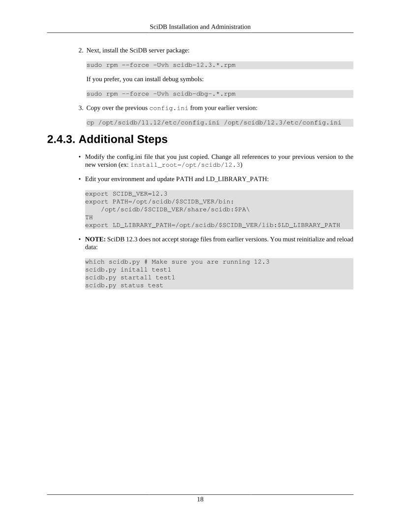
2. Next, install the SciDB server package:
sudo rpm --force -Uvh scidb-12.3.*.rpm
If you prefer, you can install debug symbols:
sudo rpm --force -Uvh scidb-dbg-.*.rpm
3. Copy over the previous config.ini from your earlier version:
cp /opt/scidb/11.12/etc/config.ini /opt/scidb/12.3/etc/config.ini
2.4.3. Additional Steps• Modify the config.ini file that you just copied. Change all references to your previous version to the
new version (ex: install_root=/opt/scidb/12.3)
• Edit your environment and update PATH and LD_LIBRARY_PATH:
export SCIDB_VER=12.3export PATH=/opt/scidb/$SCIDB_VER/bin: /opt/scidb/$SCIDB_VER/share/scidb:$PA\THexport LD_LIBRARY_PATH=/opt/scidb/$SCIDB_VER/lib:$LD_LIBRARY_PATH
• NOTE: SciDB 12.3 does not accept storage files from earlier versions. You must reinitialize and reloaddata:
which scidb.py # Make sure you are running 12.3scidb.py initall test1scidb.py startall test1scidb.py status test

19
Chapter 3. Getting Started with SciDBDevelopment3.1. Using the iquery Client
The iquery executable is the basic command-line tool for communicating with SciDB. iquery is thedefault SciDB client used to issue AQL and AFL commands. Start the iquery client by typing iqueryat the command line when a SciDB session is active:
scidb.py startall hostnameiquery
By default, iquery opens an AQL command prompt:
AQL%
You can then enter AQL queries at the command prompt. To switch to AFL queries, use the set langcommand:
AQL% set lang afl;
AQL statements end with a semicolon (;).
To see the internal iquery commands reference type help at the prompt:
AQL% help;set - List current optionsset lang afl - Set AFL as querying languageset lang aql - Set AQL as querying languageset fetch - Start retrieving query resultsset no fetch - Stop retrieving query resultsset timer - Start reporting query setup timeset no timer - Stop reporting query setup timeset verbose - Start reporting details from engineset no verbose - Stop reporting details from enginequit or exit - End iquery session
You can pass an AQL query directly to iquery from the command line using the -q flag:
iquery -q "my AQL statement"
You can also pass a file containing an AQL query to iquery with the -f flag:
iquery -f my_input_filename
AQL is the default language for iquery. To switch to AFL, use the -a flag:
iquery -aq "my AFL statement"
Each invocation of iquery connects to the SciDB coordinator instance, passes in a query, and prints outthe coordinator instance's response. iquery connects by default to SciDB on port 1239. If you use a portnumber that is not the default, specify it using the "-p" option with iquery. For example, to use port 9999to run an AFL query contained in the file my_filename do this:

Getting Started withSciDB Development
20
iquery -af my_input_filename -p 9999
The query result will be printed to stdout. Use -r flag to redirect the output to a file:
iquery -r my_output_filename -af my_input_filename
To change the output format, use the -o flag:
iquery -o csv -r my_output_filename.csv -af my_input_filename
Available options for output format are csv, csv+, lcsv+, sparse, and lsparse. These options are describedin the following table:
Output Option Description
auto (default) SciDB array format.
csv Comma-separated values.
csv+ Comma-separated values with dimension indices.
lcsv+ Comma-separated values with dimension indices and a booleanflag attribute EmptyTag showing if a cell is empty.
sparse Sparse SciDB array format.
lsparse Sparse SciDB array format and a boolean flag attribute EmptyTagshowing if a cell is empty.
To see a list of the iquery switches and their descriptions, type iquery -h or iquery --help atthe command line. The switches are explained in the following table:
iquery Switch Option Description
-c [ --host ] host_name Host of one of the cluster instances. Default is'localhost'.
-p [ --port ] port_number Port for connection. Default is 1239.
-q [ --query ] query Query to be executed.
-f [ --query-file ] input_filename File with query to be executed.
-r [ --result ] target_filename Filename with result array data.
-o [ --format ] format Output format: auto, csv, csv+, lcsv+, sparse,lsparse. Default is 'auto'.
-v [ --verbose ] Print the debugging information. Disabled bydefault.
-t [ --timer ] Query setup time (in seconds).
-n [ --no-fetch ] Skip data fetching. Disabled by default.
-a [ --afl ] Switch to AFL query language mode. Default isAQL.
-u [ --plugins ]path Path to the plugins directory.
-h [ --help ] Show help.
-V [ --version ] Show version information.
ignore-errors Ignore execution errors in batch mode.
The iquery interface is case sensitive.

Getting Started withSciDB Development
21
3.2. iquery ConfigurationYou can use a configuration file to save and restore your iquery configuration. The file is stored in~/.config/scidb/iquery.conf. Once you have created this file it will load automatically thenext time you start iquery. The allowed options are:
host Host name for the cluster instance. Default is localhost.
port Port for connection. Default is 1239.
afl Start the session with the AFL command line.
timer Report query run-time (in seconds).
verbose Print debug information.
format Set the format of query output. Options are csv, csv+, lcsv+, sparse, and lsparse.
plugins Path to the plugins directory.
For example, your iquery.conf file might look like this:
{"host":"myhostname","port":9999,"afl":true,"timer":false,"verbose":false,"format":"csv+","plugins":"./plugins"}
The opening and closing braces at the beginning and end of the file must be present and each entry (exceptthe last one) should be followed by a comma.
3.3. Example iquery sessionThis section demonstrates how to use iquery to perform simple array tasks like:
• Create a SciDB array
• Prepare an ASCII file in the SciDB dense load file format
• Load data from that file into the array.
• Execute basic queries on the array.
• Join two arrays containing related data.
The are more detailed examples on creating a SciDB array in the chapter "Creating and Removing SciDBArrays."
The following example creates an array, generates random numbers and stores them in the array, and savesthe array data into a csv-formatted file.
1. Create an array called random_numbers with:
• 2 dimensions, x = 9 and y = 10

Getting Started withSciDB Development
22
• One double attribute called num
• Random numerical values in each cell
iquery -aq "store(build(<num:double>[x=0:8,1,0, y=0:9,1,0], random()),random_numbers)"
2. Save the values in random_numbers in csv format to a file called /tmp/random_values.csv:
iquery -o csv -r /tmp/random_values.csv -aq "scan(random_numbers)"
The following example creates an array, loads existing csv data into the array, performs simple conversionson the data, joins two arrays with related data set, and eliminates redundant data from the result.
1. Create an array, target, in which you are going to place the values from the csv file:
iquery -aq "create array target <type:string,mpg:double>[x=0:*,1,0]"
2. Starting from a csv file, prepare a file to load into a SciDB array. Use the file datafile.csv, which iscontained in the doc/user/examples/ directory of your SciDB installation:
Type,MPGTruck, 23.5Sedan, 48.7SUV, 19.6Convertible, 26.8
3. Convert the file to SciDB format with the command csv2scidb:
csv2scidb -p SN -s 1 < doc/user/examples/datafile.csv > output_path/datafile.scidb
Note: csv2scidb is a separate data-preparation utility provided with SciDB. To see all optionsavailable for csv2scidb, type csv2scidb --help at the command line.
4. Use the load command to load the SciDB-formatted file you just created into target:
iquery -aq "load(target, 'output_path/datafile.scidb')"[("Truck",23.5),("Sedan",48.7),("SUV",19.6),("Convertible",26.8)]
You will need to use the full pathname for output_path. For example, if the filedatafile.scidb is located in /home/username/files, you should use the string '/home/username/files/datafile.csv' for the load function argument.
5. By default, iquery always re-reads or retrieves the data that has just written to the array. To suppressthe print to screen when you use the load command, use the -n flag in iquery:
iquery -naq "load(target, '/output_path/datafile.scidb')"
6. Now, suppose you want to convert miles-per-gallon to kilometers per liter. Use the apply function toperform a calculation on the attribute values mpg:
iquery -aq "apply(target,kpl,mpg*.4251)"
[("Truck",23.5,9.98985),("Sedan",48.7,20.7024),

Getting Started withSciDB Development
23
("SUV",19.6,8.33196),("Convertible",26.8,11.3927)]
Note that this does not update target. Instead, SciDB creates an result array with the new calculatedattribute kpl. To create an array containing the kpl attribute, use the store command:
iquery -aq "store(apply(target,kpl,mpg*.4251),target_new)"
7. Suppose you have a related data file, datafile_price.csv:
Make,Type,PriceHanda,Truck,26700Tolona,Sedan,31000Gerrd, SUV,42000Maudi,Convertible,45000
You want to add the data on price and make to your array. Use csv2scidb to convert the file to SciDBdata format:
csv2scidb -p SSN -s 1 < doc/user/examples/datafile_price.csv > output_path/datafile_price.scidb
Create an array called storage:
iquery -aq "create array storage<make:string, type:string, price:int64>[x=0:*,1,0]"
Load the datafile_price.scidb file into storage:
iquery -naq "load(storage, '/tmp/datafile_price.scidb')"
8. Now, you want to combine the data in these two files so that each entry has a make, and model, a price,an mpg, and a kpl. You can join the arrays, with the join operator:
iquery -aq "join(storage,target_new)"[("Handa","Truck",26700,"Truck",23.5,9.98985),("Tolona","Sedan",31000,"Sedan",48.7,20.7024),("Gerrd"," SUV",42000,"SUV",19.6,8.33196),("Maudi","Convertible",45000,"Convertible",26.8,11.3927)]
Note that attributes 2 and 4 are identical. Before you store the combined data in an array, you want toget rid of duplicated data.
9. You can use the project operator to specify attributes in a specific order:
iquery -aq project(target_new,mpg,kpl)[(23.5,9.98985),(48.7,20.7024),(19.6,8.33196),(26.8,11.3927)]
Attributes that are not specified are not included in the output.
10. Use the join and project operators to put the car data together. For easier reading, use csv as thequery output format:
iquery -o csv -aq "join(storage,project(target_new,mpg,kpl))"make,type,price,mpg,kpl"Handa","Truck",26700,23.5,9.98985"Tolona","Sedan",31000,48.7,20.7024

Getting Started withSciDB Development
24
"Gerrd"," SUV",42000,19.6,8.33196"Maudi","Convertible",45000,26.8,11.3927

25
Chapter 4. Creating and RemovingSciDB Arrays
SciDB organizes data as a collection of multidimensional arrays. Just as the relational table is the basis ofrelational algebra and SQL, the multidimensional array is the basis for SciDB.
A SciDB database is organized into arrays that have:
• A name. Each array in a SciDB database has an identifier that distinguishes it from all other arrays inthe same database.
• A schema, which is the array structure. The schema contains array attributes and dimensions.
1. Each attribute contains data being stored in the array's cells. A cell can contain multiple attributes.
2. Each dimension consists of a list of index values. At the most basic level the dimension of an arrayis represented using 64-bit unsigned integers. The number of index values in a dimension is referredto as the dimension's size.
4.1. Create an ArrayThe AQL CREATE ARRAY statement creates a new array and specifies the array schema. The syntaxof the CREATE ARRAY statement for a bounded array is:
CREATE ARRAY array_name <attributes> [dimensions]
The arguments for the CREATE ARRAY statement are as follows:
array_name The array name that uniquely identifies the array in the database.The maximum length of an array name is 1024 bytes. Array namesmay not contain the characters @ , :, or dot (.) as these charactersare reserved for internal SciDB operations.
attributes The array attributes contain the actual data. You specify an attributewith:
• Attribute name: Name of an attribute. The maximum length ofan attribute name is 1024 bytes. No two attributes in the samearray can share a name.
• Attribute type: Type identifier. One of the data types supportedby SciDB. Use the list('types') command to see the listof available data types.
• NULL (optional): Users can specify 'NULL' to indicate attributesthat are allowed to contain null values. If this keyword is notused, all attributes must be non null, i.e. they cannot be assignedthe special null value. If the user does not specify a value for suchan attribute, SciDB will automatically substitute a default value.
• DEFAULT (optional): Allows the user to specify the value tobe automatically substituted when a non NULL attribute lacks a

Creating and Removing SciDB Arrays
26
value. If unspecified substitution uses system defaults for varioustypes (0 for numeric types and "" for string). Note that if theattribute is declared as NULL, this clause is ignored.
dimensions Dimensions form the coordinate system for the array. The numberof dimensions in an array is the number of coordinates or indicesneeded to specify an array cell. You specify dimensions with:
• Dimension name: Each dimension has a name. Just likeattributes, each dimension must be named, and dimension namescannot be repeated in the same array. The maximum length ofa dimension name is 1024 bytes. Optionally, you may want tocreate a noninteger dimension. In this case, you will need tospecify the dimension data type in the name argument like this:dimension_name(dimension_dataype).
• Dimension start: The starting coordinate of a dimension. Thedefault data type is 64-bit integer. If you created a nonintegerdimension, this argument is omitted.
• Dimension end or *: The ending coordinate of a dimension, or *if unbounded. The default data type is 64-bit integer for boundeddimensions.
• Dimension chunk size: Number of elements per chunk.
• Dimension chunk overlap: Number of overlapping cells from aneighboring chunk.
The AQL CREATE ARRAY statement creates an array with specified name and schema. This statementcreates an array:
AQL% CREATE ARRAY A <x: double, err: double> [i=0:99,10,0, j=0:99,10,0];
The array this statement created has:
• Array name A
• An array schema with:
1. Two attributes: one with name x and type double and one with name err and type double
2. Two dimensions: one with name i, starting coordinate 0, ending coordinate 99, chunk size 10, andchunk overlap 0; one with name j, starting coordinate 0, ending coordinate 99, chunk size 10, andchunk overlap 0.
This statement creates a different array:
AQL% CREATE ARRAY B <val:double>[sample(string)=6,6,0];
Array B has one attribute named val of type double and one dimension named sample of typestring. Dimension sample has length 6, chunk size 6, and chunk overlap 0.
To delete an array with AQL, use the DROP ARRAY statement:
AQL% DROP ARRAY A;

Creating and Removing SciDB Arrays
27
4.2. Array AttributesA SciDB array must have at least one attribute. The attributes of the array are used to store individualdata values in array cells.
For example, you may want to create a product database. A 1-dimensional array can represent a simpleproduct database where each cell has a string attribute called name, a numerical attribute called price,and a datetime attribute called sold:
AQL% CREATE ARRAY products <name:string,price:float,sold:datetime> [i=0:*,10,0];
Attributes are by default set to not null. To allow an attribute to have value NULL, add NULL to theattribute data type declaration:
AQL% CREATE ARRAY product_null <name:string NULL,price:float NULL,sold:datetime NULL> [i=0:*,10,0];
This allows the attribute to store NULL values at data load.
An attribute takes on a default value of 0 when no other value is provided. To set a default value other than0, set the DEFAULT value of the attribute. For example, this code will set the default value of priceto 100 if no value is provided:
CREATE ARRAY product_dflt <name:string, price:float default 100.0, sold:datetime>[i=0:*,10,0];
4.2.1. NULL and Default Attribute ValuesSciDB offers functionality to work with missing data. This chapter uses the data set m4x4_missing.txt,shown here:
[[(0,100),(1,99),(2,98),(3,97)],[(4),(5,95),(6,94),(7,93)],[(8,92),(9,91),(),(11,89)],[(12,88),(13),(14,86),(15,85)]]
The array m4x4_missing has two issues: the second values in the cells (1,0) and (3,1) are missing, andcell (2,2) is completely empty. You can tell SciDB how you want to handle the missing data with variousarray options.
First, consider the case of the completely empty cell, (2,2). By default, SciDB will leave empty cells emptyand replace missing attributes with 0:
CREATE ARRAY m4x4_missing <val1:double,val2:int32>[x=0:3,4,0,y=0:3,4,0];load(m4x4_missing,'/tmp/m4x4_missing.txt');
[[(0,100),(1,99),(2,98),(3,97)],

Creating and Removing SciDB Arrays
28
[(4,0),(5,95),(6,94),(7,93)],[(8,92),(9,91),(),(11,89)],[(12,88),(13,0),(14,86),(15,85)]]
To change the default value, that is, the value the SciDB substitutes for the missing data, set the defaultclause of the attribute option:
CREATE ARRAY m4x4_missing <val1:double,val2:int32 default 5468>[x=0:3,4,0,y=0:3,4,0];
[[(0,100),(1,99),(2,98),(3,97)],[(4,5468),(5,95),(6,94),(7,93)],[(8,92),(9,91),(),(11,89)],[(12,88),(13,5468),(14,86),(15,85)]]
4.2.2. Codes for Missing DataIn addition to simple single-valued NULL substitution described in the previous section, SciDB alsosupports multi-valued NULLs using the notion of missing reason codes. Missing reason codes allow anapplication to optionally specify multiple types of NULLs and treat each type differently.
For example, if a faulty instrument occasionally fails to report a reading, that attribute could be representedin a SciDB array as NULL. If an erroneous instrument reports readings that are out of valid bounds foran attribute, that may also be represented as NULL.
NULL must be represented using the token 'null' or '?' in place of the attribute value. In addition, NULLvalues can be tagged with a "missing reason code" to help a SciDB application distinguish among differenttypes of null values—for example, assigning a unique code to the following types of errors: "instrumenterror", "cloud cover", or "not enough data for statistically significant result". Or, in the case of financialmarket data, data may be missing because "market closed", "trading halted", or "data feed down".
The examples below show how to represent missing data in the load file. ? or null represent null values,and ?2 represents null value with a reason code of 2.
[[ ( 10, 4.5, "My String", 'C'), (10, 5.1, ?1, 'D'), (?2, 5.1, "Another String", ?) ...
or
[[ ( 10, 4.5, "My String", 'C'), (10, 5.1, ?1, 'D'), (?2, 5.1, "Another String", null) ...
Use the substitute operator to substitute different values for each type of NULL. For more information onNULL substitution see the SciDB Operator Reference entry for substitute.
4.3. Array DimensionsA SciDB array must have at least one dimension. Dimensions form the coordinate system for a SciDBarray. There are several special types of dimensions: dimensions with overlapping chunks, unboundeddimensions, and noninteger dimensions.

Creating and Removing SciDB Arrays
29
Note
The dimension size is determined by the range from the dimension start to end, so 0:99 and 1:100would create the same dimension size.
4.3.1. Chunk OverlapIt is sometimes advantageous to have neighboring chunks of an array overlap with each other. Overlap isspecified for each dimension of an array. For example, consider an array A with the following schema:
A<a: int32>[i=1:10,5,1, j=1:30,10,5]
Array A has has two dimensions, i and j. Dimension i has size 10, chunk size 5, and chunk overlap 1.Dimension j has size 30, chunk size 10, and chunk overlap 5. SciDB stores cells from the chunk overlaparea in both of the neighboring chunks.
Some advantages of chunk overlap are:
• Speeding up nearest-neighbor queries, where each chunk may need access to a few elements from itsneighboring chunks,
• Detecting data clusters or data features that straddle more than one chunk.
4.3.2. Unbounded DimensionsAn array dimension can be created as an unbounded dimension by declaring the high boundary as '*'.When the high boundary is set as * the array boundaries are dynamically updated as new data is added tothe array. This is useful when the dimension size is not known at CREATE ARRAY time. For example,this statement creates an array named open with two dimensions:
• Bounded dimension I of size 10, chunk size 10, and chunk overlap 0
• Unbounded dimension J of size *, chunk size 10, and chunk overlap 0.
AQL% CREATE ARRAY open <val:double>[I=0:9,10,0,J=0:*,10,0];
4.3.3. Noninteger Dimensions and Mapping ArraysBasic arrays in SciDB use the int64 data type for dimensions. SciDB also supports arrays with nonintegerdimensions. These arrays map dimension values of a declared type to an internal int64-array position.Mapping is done through special mapping arrays internal to SciDB. Such arrays are useful when you aretransforming data into multidimensional format where some dimensions represent factors or categories.
For example, the array D has a noninteger dimension named ID:
AQL% SELECT * FROM show(D);
[("D <val:int64 ,empty_indicator:indicator > [ID(string)=10,5,0]")]
The dimension indices of ID are:
AQL% SELECT * FROM D:ID;
[("sample-1"),("sample-10"),("sample-2"),("sample-3"),

Creating and Removing SciDB Arrays
30
("sample-4"),("sample-5"),("sample-6"),("sample-7"),("sample-8"),("sample-9")]
The values of the attribute val of D are:
AQL% SELECT * FROM D;
[(0),(90),(2),(6),(12),(20),(30),(42),(56),(72)]
Note
In the current version of SciDB, it is not possible to load data directly from an external file intoa mapping array.
4.4. Changing Array NamesAn array name is used to identify an array in the current SciDB namespace. You can use the AQLSELECT ... INTO statement to rename an array.
AQL% SELECT * INTO new_A FROM A;
This means that both A and new_A are in the current SciDB namespace. To change an array name andremove the old array name from the current SciDB namespace, use the rename command:
AFL% rename(new_A, A_backup);
You can use the cast command to change the name of the array, array attributes, and array dimensions.A single cast can be used to rename multiple items at once, for example, one or more attribute names and/or one or more dimension names. The input array and template arrays should have the same numbers andtypes of attributes and the same numbers and types of dimensions.
AQL% SELECT * FROM show(A);
[("A<x:double ,err:double > [i=0:99,10,0,j=0:99,10,0]")]
This query creates an array new_A with attributes val1 and val2 and dimensions x and y:
AQL% SELECT * INTO new_A FROM cast(A,<val1:double,val2:double>[x=0:99,10,0,y=0:99,10,0]")];
4.5. Database Design
4.5.1. Selecting Dimensions and AttributesAn important part of SciDB database design is selecting which values will be dimensions and whichwill be attributes. Dimensions form a coordinate system for the array. Adding dimensions to an arraygenerally improves the performance of many types of queries by speeding up access to array data. Hence,the choice of dimensions depends on the types of queries expected to be run. Some guidelines for choosingdimensions are:
• Dimensions provide selectivity and efficient access to array data. Any coordinate along which selectionqueries must be performed constitutes a good choice of dimension. If you want to select data subject

Creating and Removing SciDB Arrays
31
to certain criteria (for example, all products of price greater than $100 whose brand name is longerthan six letters that were sold before 01/01/2010) you may want to design your database such that thecoordinates for those parameters are defined by dimensions.
• Array aggregation operators including group-by, window, or grid aggregates specify coordinates alongwhich grouping must be performed. Such values must be present as dimensions of the array. For spatialand temporal applications, the space or time dimension is a good choice for a dimension.
• In the case of 2-dimensional arrays common in linear algebra applications, rows represent observationsand columns represent variables, factors, or components. Matrix operations such as multiply,covariance, inverse, and best-fit linear equation solution are often performed on a 2-dimensional arraystructure.
In the absence of these factors, choosing to represent values as attributes is generally a good idea. However,SciDB offers the flexibility to transform data from one array definition to another even after it has beenloaded. This step is referred to as redimensioning the array and is especially useful when the same dataset must be used for different types of analytic queries. Redimensioning is used to transform attributesto dimensions and vice-versa. Redimensioning an array is explained in the chapter "Changing ArraySchemas."
4.5.2. Chunk Size SelectionThe selection of chunk size in a dimension plays an important role in how well you can query your data.If a chunk size is too large or too small, it will negatively impact performance.
To optimize performance of your SciDB array, you want chunks to contain on order of 10 to 20 MB ofdata. So, for example, if your data set consists entirely of double-precision numbers, you would want achunk size that contains somewhere between 500,000 and 1 million elements (assuming 8 bytes for everydouble-precision number).
When a multiattribute SciDB array is stored, the array attributes are stored in different chunks, a processknown as vertical partitioning. This is a consideration when you are choosing a chunk size. The size ofan individual cell, or the number of attributes per cell, does not determine the total chunk size. Rather,the number of cells in the chunk is the number to use for determining chunk size. For arrays where everydimension has a fixed number of cells and every cell has a value you can do a straightforward calculationto find the correct chunk size.
When the density of the data in a data set is highly skewed, that is, when the data is not evenlydistributed along array dimensions, the calculation of chunk size becomes more difficult. The calculationis particularly difficult when it isn't known at array creation time how skewed the data is. In this case, youmay want to use SciDB's repartitioning functionality to change the chunk size as necessary. Repartitioningan array is explained in the chapter "Changing Array Schemas."

32
Chapter 5. Loading DataThe key part of setting up your SciDB array is loading your data. This chapter begins by explaining thesimplest way to prepare and load a data file. Later, this chapter explains more complicated load scenariossuch as sparse loading and parallel loading. Finally, this chapter shows you how to round-trip your databy saving it from a SciDB array back out into a csv file.
The array data model is core to SciDB. When you define a schema for an array you specify which aspectsof your data you want to be dimensions and which aspects you want to be attributes based on how youwant to conceptualize, access and operate on the data. Before loading data, you have to create an arrayto load your data into. Refer to the chapter "Creating and Removing SciDB Arrays" for how to create aSciDB array.
5.1. Simple Data LoadingThis section describes how to do a simple data load procedure. The steps in simple data loading are:
1. Save your data in comma-separated value (csv) format.
2. Use the csv2scidb command to create a SciDB-formatted load file.
3. Create a 1-dimensional SciDB array to load the data into.
4. Use the LOAD statement to load the data from the SciDB-formatted file into the array.
Consider the 20-line, csv-formatted file num_data.csv, the first few lines of which are shown here:
val,err1.48306e+09,15.80814e+08,11.51079e+09,11.16154e+09,11.42655e+09,11.06341e+09,1
This file has two entries per row, where the entries are labelled val and err. To prepare this filefor loading into a SciDB array, use the command csv2scidb. The csv2scidb command takesmulticolumn csv data and transforms it into 1-dimensional arrays with one attribute for every comma-delimited column. The syntax of csv2scidb is:
csv2scidb [options] < input-file > output-file
Note
csv2scidb is accessed directly at the command-line and not through the iquery client. Tosee the options for csv2scidb, type csv2scidb --help at the command line. The optionsfor csv2scidb are:
-v version of tool-i PATH input file-o PATH output file-a PATH appended output file

Loading Data
33
-c INT length of chunk-f INT starting chunk number-d char delimiter,default is , (comma)-p STR type pattern, N number, S string, s nullable string, C char-q Quote the input line exactly, simply wrap it in ()-s INT skip N lines at the beginning of the file
This code will transform num_data.csv to SciDB load file format:
csv2scidb -s 1 -p N < num_data.csv > num_data.scidb
The -s flag specifies the number of lines to skip at the beginning of the file. Since the file has a header,you can strip that line, and provide that information as attribute names. The -p flag specifies the type ofdata you are loading. Possible values are N (number), S (string), s (nullable string), and C (char).
The file num_data.scidb looks like this:
[(1.48306e+09,1),(5.80814e+08,1),(1.51079e+09,1),(1.16154e+09,1),(1.42655e+09,1),(1.06341e+09,1),(4.9253e+08,1),(5.6065e+08,1),(1.60886e+08,2),(1.37844e+09,1),(4.08495e+08,1),(5.65393e+07,1),(1.47646e+09,1),(9.52609e+08,1),(1.8548e+09,1),(1.42396e+09,1),(1.75107e+09,1),(1.52007e+09,1),(5.4882e+08,1),(7.28928e+08,1)]
The square braces show the beginning and end of the array dimension. The parentheses show the cells ofthe array. There are commas between attributes in cells and cells in the dimension.
To create an array for this data, create an array with 1-dimension. The original data set had two columnheaders of val and err, so you can name the attributes val and err:
AQL% CREATE ARRAY num_data <val:double,err:double>[i];
To load the data into the array num_data, use a LOAD statement:
AQL% LOAD num_data FROM 'base-path/doc/user/examples/num_data.scidb';
The base-path is the directory where your SciDB source files are stored.

Loading Data
34
5.2. Data with Special ValuesSuppose you have a load file that is missing some values, like this file, v4.scidb:
[ (0,100),(1,99),(2,),(3,97)]
The load file v4.scidb has a missing value in the third cell. If you create an array and load this dataset, SciDB will substitute 0 for the missing value:
AQL% CREATE ARRAY v4 <val1:int8,val2:int8>[i=0:3,4,0];AQL% LOAD v4 FROM '/examples/v4.scidb';
[(0,100),(1,99),(2,0),(3,97)]
To change the default value, that is, the value the SciDB substitutes for the missing data, set the DEFAULTattribute option. This code creates an array v4_dflt with default attribute value set to 111:
AQL% CREATE ARRAY v4_dflt <val1:int8,val2:int8 default 111>[i=0:3,4,0];AQL% LOAD v4_dflt FROM '/examples/v4.scidb';
[(0,100),(1,99),(2,111),(3,97)]
Load files may also contain null values, such as in this file, v4_null.scidb:
[ (0,100),(1,99),(2,null),(3,97)]
To preserve null values at load time, add the NULL option to the attribute type:
AQL% CREATE ARRAY v4_null<val1:int8,val2:int8 NULL> [i=0:3,4,0];AQL% LOAD v4_null FROM '/example/v4_null.scidb';
[(0,100),(1,99),(2,null),(3,97)]
5.3. Sparse Load FormatThe sparse load format allows a large number of cells to be unspecified. In the sparse load format, data islisted by chunks. Chunks are delimited by two square brackets. There are semicolons between chunks.
[[chunk1]];[[chunk2]];

Loading Data
35
Within each chunk, the data is organized as a list of cells. Each cell includes the coordinate indices of thecell in curly braces and the attributes of the cell (separated by commas) in parentheses.
[[{index1,index2,...} (attribute1,attribute2,...), ... {indexm,indexn} (attribute1m,attribute2n)]];
For example, a load file for a diagonal 2-D array with two chunks looks like this:
[[{0,0}(0,'A'),{1,1}(1,'B'),{2,2}(2,'C'),{3,3}(3,'D')]];[[{4,4}(6,'G'),{5,5}(7,'P'),{6,6}(9,'H')]]
This data is stored like this:
Tip
In addition to storing the data, LOAD operator returns the data back to the client (or next operatorin the query). When the data set is very large, you may want to suppress the query output.The iquery executable that accompanies SciDB includes the -n option for this purpose. See"Getting Started with SciDB Development" for how to use iquery.
5.3.1. Sparse Load ChunksConsider a load file like this:
[[{0,0} (11),{1,0} (21),{0,1} (12)]];[[{0,2} (13)]];[[{2,0} (31),{3,0} (41),{2,1} (32),{3,1} (42)]];[[{2,2} (33),{3,3} (44)]];[[{7,0} (81),{6,1} (72),{7,1} (82)]];

Loading Data
36
[[{6,2} (73),{7,2} (83),{7,3} (84)]];[[{8,0} (91)]];[[{8,2} (93),{8,3} (94)]]
The chunk distribution in the load file requires that the array have chunks of size 2 in the first dimensionand chunks of size 2 in the second dimension. The array schema for this load file is:
<attribute:int16>[x=0:8,2,0,y=0:3,2,0];
5.4. Parallel LoadThe simple data loading procedure serially loads all the data from a single load file. You can set up parallelloading for much faster loading. Parallel loading is more complex because it requires the creation ofmultiple load files which are chunk-size specific. That is, they are custom constructed around a knownchunk size and have to be written with embedded chunk identifiers.
The optional id parameter instructs the LOAD command to open and load data from a particular instanceof SciDB. Possible id values are:
id Value Description
0 Coordinator
1,2, ..., N id of the instance that should perform the load where N is the number ofinstances in the cluster.
–1 All instances in the cluster. The file path is assumed to be the same at allinstances. If an instance cannot open the data file, the load will continueafter logging a warning.
For parallel load, each instance must be given distinct chunks. To do this, chunks in the load file must beprefixed with a distinct chunk header that lists the starting dimension values of the chunk.
If your SciDB cluster has 4 instances (with identifiers 1, 2, 3, and 4) and there are 20 chunks, you canplace chunks 1–5 on instance 1, chunks 6–10 on instance 2, and so on. The following load command willsimultaneously load all 20 chunks into the array and complete 4 times faster.
AFL% load (Array, '/tmp/load.data', -1);
5.5. Saving Data from a SciDB Array to a FileYou can save all or part of the data that is contained in a SciDB array to a file. You can use a SELECTstatement with the SAVE clause to save an entire array. For example, consider the following arrayrandom_numbers:
AQL% CREATE ARRAY random_numbers <val:double>[i=0:99,100,0];

Loading Data
37
AQL% SELECT * INTO random_numbers FROM build(random_numbers,random());
You can save the values stored in the array random_numbers to a file with the following query:
AQL% SAVE random_numbers INTO '/tmp/random_data.txt';
This statement saves a SciDB-formatted file called random_data.txt.
To save the data to csv format, set the iquery output option to csv:
% iquery -o csv -q "SAVE random_numbers INTO '/tmp/random_data.csv';"
val,val_rand1,9396180952,10116557743,36206192104,23170573325,61372608456,107713279807,44965693368,103642903289,230951380510,1398261690
Note
You will need to enter your iquery statement directly at the command line to change the outputoption to csv. Type exit; at the AQL% prompt to stop the current iquery session.

38
Chapter 6. Basic Array Tasks6.1. Selecting Data From an Array
AQL's Data Manipulation Language (DML) provides queries to access and operate on array data. Thebasis for selecting data from a SciDB array is the AQL SELECT statement with INTO, FROM, and WHEREclauses. The syntax of the SELECT statement is:
SELECT list | * [INTO target_array] FROM array_expression | source_array [WHERE expression]
The arguments for the statement are:
list | * SELECT list can select individual attributes and dimensions, aswell as constants and expressions. The wildcard character * meansselect all attributes.
target_array The INTO clause can create an array to store the output ofthe query. The target array may also be a pre-existing array in thecurrent SciDB
array_expression |source_array
The FROM clause takes a SciDB array as argument. Thearray_expression argument is an expression or subquery thatreturns an array result. The source_array is an array in thecurrent SciDB namespace from which data is being selected.
expression The expression argument of the WHERE clause allows to youspecify parameter that filter the query.
6.1.1. The SELECT StatementAQL expressions in the SELECT list or the WHERE clause are standard expressions over the attributesand dimensions of the array. The simplest SELECT statement is SELECT *, which selects all datafrom a specified array or array result. Consider two arrays, A and B:
AQL% CREATE ARRAY A <val_a:double>[i=0:9,10,0];AQL% CREATE ARRAY B <val_b:double>[j=0:9,10,0];
These arrays contain data. To see all the data in the array, you can use a SELECT * statement with thescan command. The scan(A) command returns a SciDB array result containing the values of the arraydata in A. By using scan(A) with a SELECT * statement, the query will return the entire array resultof scan(A):
AQL% SELECT * FROM scan(A);
[(1),(2),(3),(4),(5),(6),(7),(8),(9),(10)]
AQL% SELECT * FROM scan(B);
[(101),(102),(103),(104),(105),(106),(107),(108),(109),(110)]

Basic Array Tasks
39
The show command returns an array result containing an array's schema. To see the entire schema, usea SELECT * statement with the show command:
AQL% SELECT * FROM show(A);
[("A<val_a:double> [i=0:9,10,0]")]
AQL% SELECT * FROM show(B);
[("B<val_b:double> [j=0:9,10,0]")]
To refine the result of the SELECT statement, use an argument that specifies part of an array result.SELECT can take array dimensions or attributes as arguments:
SELECT j FROM B;SELECT val_b FROM B;
The SELECT statement can also take an expression as an argument. For example, you can scale attributevalues by a certain amount:
AQL% SELECT val_b/10 FROM B;
[(10.1),(10.2),(10.3),(10.4),(10.5),(10.6),(10.7),(10.8),(10.9),(11)]
The WHERE clause can also use built-in functions to create expressions. For example, you can choosejust the middle three cells of array B with the greater-than and less-than functions with the and operator:
SELECT j FROM B WHERE j > 3 and j < 7;
[(),(),(),(),(4),(5),(6),(),(),()]
You can also select an expression of the attribute values for the middle three cells of B by providing anexpression for the argument of both SELECT and WHERE . For example, this statement returns thesquare root of the middle three cells of array B:
SELECT sqrt(val_b) FROM B WHERE j>3 and j<7;
[(),(),(),(),(10.247),(10.2956),(10.3441),(),(),()]
The FROM clause can take an array or any operation that outputs an array as an argument. The INTOclause stores the output of a query.
6.2. Array JoinsA join combines two or more arrays typically as a preprocessing step for subsequent operations. Thesimplest type of join is for two arrays with the same number of dimensions, same dimension startingcoordinates, and same chunk size.
The syntax of a simple join statement is:
SELECT expression INTO target_array FROM src_array
The natural join of these arrays joins the attributes:
SELECT * FROM A,B;

Basic Array Tasks
40
This join produces:
[(1,101),(2,102),(3,103),(4,104),(5,105),(6,106),(7,107),(8,108),(9,109),(10,110)]
You can store the output using the INTO clause. For example, this code will store the attribute-attributejoin of A and B in array C:
AQL% SELECT * INTO C FROM A,B;
Arrays do not need to have the same number of attributes to be compatible as long as the dimension startingindices, chunk sizes, and chunk overlaps are the same. For example, you can join the two-attribute arrayC with the one-attribute array B:
AQL% SELECT * INTO D FROM C,B;
This produces array D with the following schema:
[("D<val_a:double,val_b:double,val_b_2:double>[i=0:9,10,0]")]
If two arrays have an attribute with the same name, you can select the attributes to use with array dotnotation:
AQL% SELECT C.val_b + D.val_b FROM C,D;
The JOIN ... ON predicate calculates the multidimensional join of two arrays after applying theconstraints specified in the ON clause. The ON clause lists one or more constraints in the form of equalitypredicates on dimensions or attributes. The syntax is:
SELECT list | * [INTO target_array] FROM array_expression | source_array JOIN expression | attribute ON dimension | attribute
A dimension-dimension equality predicate matches two compatible dimensions, one from each input. Theresult of this join is an array with higher number of dimensions—combining the dimensions of both itsinputs, less the matched dimensions. If no predicate is specified, the result is the full cross product array.
An attribute predicate in the ON clause is used to filter the output of the multidimensional array.
For example, consider a 2-dimensional array m3x3schema and attributes values:
[("m3x3<a:double> [i=1:3,3,0,j=1:3,3,0]")][[(4),(5),(6)],[(7),(8),(9)],[(10),(11),(12)]]
Now consider also a 1-dimensional array vector3 schema and attribute values:
[("vector3<b:double> [k=1:3,3,0]")][(21),(20.5),(20.3333)]

Basic Array Tasks
41
A dimension join returns a 2-dimensional array with coordinates {i,j} in which the cell at coordinate{i,j} combines the cell at {i,j} of m3x3 with the cell at coordinate {k=j} of vector3:
AQL% SELECT * FROM m3x3 JOIN vector3 ON m3x3.j = vector3.k;
[[(4,21),(5,20.5),(6,20.3333)],[(7,21),(8,20.5),(9,20.3333)],[(10,21),(11,20.5),(12,20.3333)]]
6.3. AliasesAQL provides a way to refer to arrays and array attributes in a query via aliases. These are useful whenusing the same array repeatedly in an AQL statement, or when abbreviating a long array name. Aliasesare created by adding an "as" to the array or attribute name, followed by the alias. Future references to thearray can then use the alias. Once an alias has been assigned, all attributes and dimensions of the array canuse the fully qualified name using the dotted naming convention.
AQL% SELECT data.i*10 FROM A AS data WHERE A.i < 5;
[(0),(10),(20),(30),(40),(),(),(),(),()]
6.4. Nested SubqueriesYou can nest AQL queries to refine query results.
For example, you can nest SELECT statements before a WHERE clause to select a subset of thequery output. For example, this query
1. Sums two attributes from two different arrays and stores the output in an alias,
2. Selects the cells with indices greater than 5, and
3. Squares the result.
AQL% SELECT pow(c,2) FROM (SELECT A.val_a + B.val_b AS c FROM A,B) WHERE i > 5;
[(),(),(),(),(),(),(12996),(13456),(13924),(14400)]
6.5. Data SamplingSciDB provides operations to sample array data. The bernoulli command allows you to select a subsetof array cells based upon a given probability. For example, you can use the bernoulli operator torandomly sample data from an array one element at a time. The syntax of bernoulli is:
bernoulli(array, probability:double [, seed:int64])
The sample command allows you to randomly sample data one array chunk at a time:
sample(array, probability:double [, seed:int64])
The probability is a double between 0 and 1. The commands work by generating a random number for eachcell or chunk in the array and scaling it to the probability. If the random number is within the probability,

Basic Array Tasks
42
the cell/chunk is included. Both commands allow you to produce repeatable results by seeding the randomnumber generator. All calls to the random number generator with the same seed produce the same randomnumber. Seeds must be a 64-bit integer.

43
Chapter 7. AggregatesSciDB supports commands to group data from an array and calculate summaries over those groups. Thesecommands are called aggregates. SciDB provides the following types of aggregates based on how datais grouped:
• Grand aggregates compute aggregates over entire arrays.
• Group-by aggregates compute summaries by grouping array data by dimension values.
• Grid aggregates compute summaries for nonoverlapping subarrays.
• Window aggregates compute summaries over a moving window in an array.
This chapter uses example arrays m4x4 and m4x4_2attr, which have the following schemas and containthe following values:
AFL% show(m4x4);
[("m4x4<attr1:double> [x=0:3,4,0,y=0:3,4,0]")]
AFL% scan(m4x4);
[[(0),(1),(2),(3)],[(4),(5),(6),(7)],[(8),(9),(10),(11)],[(12),(13),(14),(15)]]
AFL% show(m4x4_2attr);
[("m4x4_2attr<attr1:double,attr2:double> [x=0:3,4,0,y=0:3,4,0]")]
AFL% scan(m4x4_2attr);
[[(0,0),(1,2),(2,4),(3,6)],[(4,8),(5,10),(6,12),(7,14)],[(8,16),(9,18),(10,20),(11,22)],[(12,24),(13,26),(14,28),(15,30)]]
SciDB offers the following built-in aggregates.
Aggregate Function Definition
avg Average value
count Number of nonempty elements (array count) and non-null elements(attribute count).
max Largest value
min Smallest value
sum Sum of all elements

Aggregates
44
stdev Standard deviation
var Variance
7.1. Grand AggregatesGrand aggregates in SciDB calculate aggregates or summaries of attributes across an entire array. Thesyntax of the SELECT statement with a summary clause is:
AQL% SELECT aggregate(attribute),function(attribute),... INTO dst-array FROM src-array | array-expression WHERE where-expression
The output is a SciDB array with one attribute named for the summary type in the query and arraydimensions determined by the size and shape of the result.
For example, to select the maximum and the minimum values of the attribute attr1 of the array m4x4:
AQL% SELECT max(attr1),min(attr1) FROM m4x4;
[(15,0)]
You can store the output of a query into a destination array, m4x4_max_min with an INTO clause:
AQL% SELECT max(attr1),min(attr1) INTO m4x4_max_min FROM m4x4;
The destination array m4x4_max_min has schema:
[("m4x4_max_min<max:double NULL,min_1:double NULL> [i=0:0,1,0]")]
To select the maximum value from the attribute val of m4x4_2attr and the minimum value from theattribute val2 of m4x4_2attr:
AQL% SELECT max(attr2),min(attr) FROM m4x4_2attr;
[(30,0)]
Note
In the special case of a one-attribute array, you can omit the attribute name. For example, toselect the maximum value from the attribute attr1 of the array m4x4, use the AQL SELECTstatement:
AQL% SELECT max(m4x4);
[(15)]
The AFL aggregate operator also computes grand aggregates. To select the maximum value from theattribute val of m4x4_2attr and the minimum value from the attribute val2 of m4x4_2attr:
AFL% aggregate(m4x4_2attr, max(attr2),min(attr1));

Aggregates
45
[(30,0)]
SciDB functions exclude null-valued data. For example, consider the following array m4x4_null:
[[(null),(null),(null),(null)],[(null),(null),(null),(null)],[(0),(0),(0),(0)],[(null),(null),(null),(null)]]
The syntaxes count(attr1) and count(*) return different results:
AQL% SELECT count(attr1) AS a, count(*) AS b FROM m4x4_null;
[(4,16)]
One syntax, count(attr1), shows only cells that have values that are not NULL. The other syntax,count(*), counts all of the present cells (both NULL and not NULL).
7.2. Group-By AggregatesGroup-by aggregates allow you to group array data by array dimensions and summarize the data in thosegroups.
AQL GROUP BY aggregates take a list of dimensions as the grouping criteria and compute the aggregatefunction for each group. The result is an array containing only the dimensions specified in the GROUPBY clause and a single attribute per specified aggregate call. The syntax of the SELECT statementfor a group-by aggregate is:
SELECT function(attribute), function(attribute), ... INTO dst-array FROM src-array | array-expression WHERE where-expression GROUP BY dimension, dimension, ...;
For example, this query selects the maximum value from the attribute val of array m4x4 grouped bydimension x:
AQL% SELECT max(attr1) FROM m4x4 GROUP BY x;
This query outputs:
[(3),(7),(11),(15)]
which has schema:
<max:double NULL> [x=0:3,4,0]
This query selects the maximum values from attribute attr1 of array m4x4 grouped by dimension y:
AQL% SELECT max(attr1) FROM m4x4 GROUP BY y;
[(12),(13),(14),(15)]

Aggregates
46
The AFL aggregate operator takes dimension arguments to support group-by functionality. This queryselects the maximum values from the dimension y and attribute val from the array m4x4 using AFL:
AFL% aggregate(m4x4, max(attr1),y);
[(12),(13),(14),(15)]
7.3. Grid AggregatesA grid aggregate selects nonoverlapping subarrays from an existing array and calculates an aggregate ofeach subarray. For example, if you have a 4x4 array, you can create 4 nonoverlapping 2x2 regions andcalculate an aggregate for those regions. The array m4x4 would be divided into 2x2 grids as follows:
The syntax of a grid aggregate statement is:
AQL% SELECT function(attribute), function(attribute), ... INTO dst-array FROM src-array | array-expression WHERE where-expression REGRID dimension1-size, dimension2-size, ...;
For example, this statement finds the maximum and minimum values for each of the four grids in theprevious figure:
AQL% SELECT max(attr1), min(attr1) FROM m4x4 REGRID 2,2;
[[(5,0),(7,2)],[(13,8),(15,10)]]
This output has schema:
<max:double NULL,min_1:double NULL> [x=0:1,2,0,y=0:1,2,0]
In AFL, you can use the regrid operator:
AFL% regrid(m4x4, 2,2, max(attr1),min(attr1));
[[(5,0),(7,2)],

Aggregates
47
[(13,8),(15,10)]]
7.4. Window AggregatesWindow aggregates allow you to specify groups with a moving window. The window is defined by a sizein each dimension. The window centroid starts at the first array element. The grouping starts at the firstelement of the array and moves in stride-major order from the lowest to highest value in each dimension.The syntax of a window aggregate statement is:
AQL% SELECT function(attribute), function(attribute), ... INTO dst-array FROM src-array | array-expression WHERE where-expression WINDOW dimension1-size, dimension2-size, ...;
For example, you can use a window to calculate a running sum for a 3x3 window on array m4x4.
In AQL, you would use this statement:
AQL% SELECT sum(attr1) FROM m4x4 WINDOW 3,3;
Which returns values:
[[(10),(18),(24),(18)],[(27),(45),(54),(39)],[(51),(81),(90),(63)],[(42),(66),(72),(50)]]
with schema:

Aggregates
48
<sum:double NULL> [x=0:3,4,0,y=0:3,4,0]
Since the window centroid starts at cell {0,0}, the region of the window that is outside the array boundaryis not counted in the aggregation. The window always returns the same dimensions as the input array. Ifthe window size is even, the query takes the preceding cells first. For example, a 1-dimensional windowsize of 4 means that the window takes the values of two 2 preceding cells, the value of the current cell,and the value of 1 cell following.
In AFL, you would use the window operator:
AFL% window(m4x4,3,3,sum(attr1));
[[(10),(18),(24),(18)],[(27),(45),(54),(39)],[(51),(81),(90),(63)],[(42),(66),(72),(50)]]

49
Chapter 8. Updating Your DataSciDB uses a "no overwrite" storage model. No overwrite means that data in an array can be updatedbut previous values can be accessed as long as the array exists in the SciDB namespace. Every time youupdate data in an array, SciDB creates a new array version, much like source control systems for softwaredevelopment.
8.1. The UPDATE ... SET statementTo update data in an existing SciDB array, use the statement:
AQL% UPDATE array SET "attr = expr", ... [ WHERE condition ];
Consider the following 2-dimensional array, m4x4:
[("m4x4<val:double> [x=0:3,4,0,y=0:3,4,0]")][[(0),(1),(2),(3)],[(4),(5),(6),(7)],[(8),(9),(10),(11)],[(12),(13),(14),(15)]]
To change every value in val to its additive inverse:
AQL% UPDATE m4x4 SET val=-val;
[[(0),(-1),(-2),(-3)],[(-4),(-5),(-6),(-7)],[(-8),(-9),(-10),(-11)],[(-12),(-13),(-14),(-15)]]
The WHERE clause lets you choose attributes based on conditions. For example, you can select just cellswith absolute values greater than 5 to set to their multiplicative inverse:
AQL% UPDATE m4x4 SET val=pow(val,-1) WHERE abs(val) > 5;
[[(0),(-1),(-2),(-3)],[(-4),(-5),(-0.166667),(-0.142857)],[(-0.125),(-0.111111),(-0.1),(-0.0909091)],[(-0.0833333),(-0.0769231),(-0.0714286),(-0.0666667)]]
8.2. Array VersionsWhen an array is updated, a new array version is created. SciDB stores the array versions. For example,in the previous section, SciDB stored every version of m4x4 created by the UPDATE command. Youcan see these versions with versions:
AQL% SELECT * FROM versions(m4x4);

Updating Your Data
50
[(1,"2012-02-03 17:20:50"),(2,"2012-02-06 14:51:20"),(3,"2012-02-06 14:52:33")]
You can see the contents of any previous version of the array by using the version number:
AQL% SELECT * FROM scan(m4x4@1);[[(0),(1),(2),(3)],[(4),(5),(6),(7)],[(8),(9),(10),(11)],[(12),(13),(14),(15)]]
Or the array timestamp:
AQL% SELECT * FROM scan(m4x4@datetime('2012-02-03 17:20:50'));[[(0),(1),(2),(3)],[(4),(5),(6),(7)],[(8),(9),(10),(11)],[(12),(13),(14),(15)]]
You can use the array version name in any query. The unqualified name of the array always refers to themost recent version as of the start of the query.

51
Chapter 9. Changing Array Schemas:Transforming Your SciDB Array
9.1. Redimensioning an ArrayA common use case for creating and loading SciDB arrays is using data from a data warehouse. This dataset may be very large and formatted as a csv file. You can use the csv2scidb utility to convert a csv fileto the 1-dimensional array format and load the file into a SciDB array. Once you have a 1-dimensionalSciDB array, you can redimension the array to convert the attributes to dimensions.
For example, suppose you have a csv file like this:
d,t,val"device-0","trial-0",0.01"device-1","trial-0",2.04"device-2","trial-0",6.09"device-3","trial-0",12.16"device-4","trial-0",20.25"device-0","trial-1",30.36"device-1","trial-1",42.49"device-2","trial-1",56.64"device-3","trial-1",72.81"device-4","trial-1",91"device-0","trial-2",111.21"device-1","trial-2",133.44"device-2","trial-2",157.69"device-3","trial-2",183.96"device-4","trial-2",212.25"device-0","trial-3",242.56"device-1","trial-3",274.89"device-2","trial-3",309.24"device-3","trial-3",345.61"device-4","trial-3",384"device-0","trial-4",424.41"device-1","trial-4",466.84"device-2","trial-4",511.29"device-3","trial-4",557.76"device-4","trial-4",606.25
This data has three columns, two of which are stings and one which is a floating-point number. The columnheaders are 'd','t',and 'val'. To load this data set, create a 1-dimensional SciDB array with three attributesand load the data into it. For this example, the array is named expo. The dimension name is i, the dimensionsize is 25, the chunk size is 5. The attributes are s, of type string, p of type string, and val of type double.
AQL% SELECT * FROM show(device_trial);
[("device_trial<d:string,t:string,val:double> [i=1:25,5,0]")]
When you examine the data, notice that it could be expressed in a 2-dimensional format like this:

Changing Array Schemas:Transforming Your SciDB Array
52
trial-0 trial-1 trial-2 trial-3 trial-4
device-0 0.01 30.36 111.21 242.56 424.41
device-1 2.04 42.49 133.44 274.89 466.84
device-2 6.09 56.64 157.69 309.24 511.29
device-3 12.16 72.81 183.96 345.61 557.76
device-4 20.25 91 212.25 384 606.25
SciDB allows you to redimension the data so that you can store it in this 2-dimensional format. First, createan array with 2 dimensions:
AFL% create array two_dim<val:double>[d(string)=5,5,0, t(string)=5,5,0];
Each of the dimensions is of size 5, corresponding to a dimension in the 5-by-5 table. Now, you can usethe redimension_store operator to redimension the array device_trial into the array two_dim:
AFL% redimension_store(device_trial, two_dim);
[[(0.01),(30.36),(111.21),(242.56),(424.41)],[(2.04),(42.49),(133.44),(274.89),(466.84)],[(6.09),(56.64),(157.69),(309.24),(511.29)],[(12.16),(72.81),(183.96),(345.61),(557.76)],[(20.25),(91),(212.25),(384),(606.25)]]
Now the data is stored so that device and trial numbers are the dimensions of the array. This means thatyou can use the dimension indices to select data from the array. For example, to select the second devicefrom the third trial, use the dimension indices:
AQL% SELECT val FROM two_dim WHERE s='device-2' and p='trial-3';
Redimensioning is a powerful tool when you want to do array aggregation along the coordinate axes of adata set. For example, you can find the average value of a trial for each device. This would be equivalentto finding the average of every row in the table:
AFL% create array Ds<av:double NULL>[d(string)=5,5,0];redimension_store(device_trial, Ds, true, avg(val) as av);
Or, you can find the average value of all the samples for a single trial. This would be equivalent to findingthe average of every column in the table:
AFL% create array Dp<av:double NULL>[d(string)=5,5,0];AFL% redimension_store(device_trial, Dp, true, avg(val) as av);
9.1.1. Redimensioning Arrays Containing Null ValuesNullable attributes cannot be transformed into dimensions. For example, consider the 1-dimensional arrayredim_missing:
AFL% show(redim_missing);scan(redim_missing);
[("redim_missing<val1:string,val2:string NULL,val3:double>

Changing Array Schemas:Transforming Your SciDB Array
53
[i=0:9,10,0]")][("0","0",1),("0","1",0.540302),("0","2",-0.416147),("0","3",-0.989992),("0","4",-0.653644),("1","null",.7),("1","1",0.841471),("1","2",0.909297),("1","3",0.14112),("1","4",-0.756802)]
Suppose you want to change the first two attributes into dimension indices and store the third attribute ina 2-dimensional array. Create an array redim_target to store the redimension results:
AFL% CREATE ARRAY redim_target <val3:double> [val1(string)=2,2,0,val2(string)=5,5,0];
The array redim_missing contains a nullable attribute and a null-valued cell. You will need to use thesubstitute operator to update redim_missing before redimensioning:
AFL% store(build(<exp1:string>[i=0:0,1,0],0),subst_array);AFL% store(substitute(redim_missing,subst_array),redim_source);
This query outputs:
[("0","0",1),("0","1",0.540302),("0","2",-0.416147),("0","3",-0.989992),("0","4",-0.653644),("1","0",.7),("1","1",0.841471),("1","2",0.909297),("1","3",0.14112),("1","4",-0.756802)]
You can now use redimension_store to turn redim_source into a 2-dimensional array:
AFL% redimension_store(redim_source,redim_target);
This query outputs:
[[(1),(0.540302),(-0.416147),(-0.989992),(-0.653644)],[(.7),(0.841471),(0.909297),(0.14112),(-0.756802)]]
9.2. Array TransformationsOnce you have created, loaded, and redimensioned a SciDB array, you may want to change some aspectof that array. SciDB offers functionality to transform the elements of the array schema (attributes anddimensions).
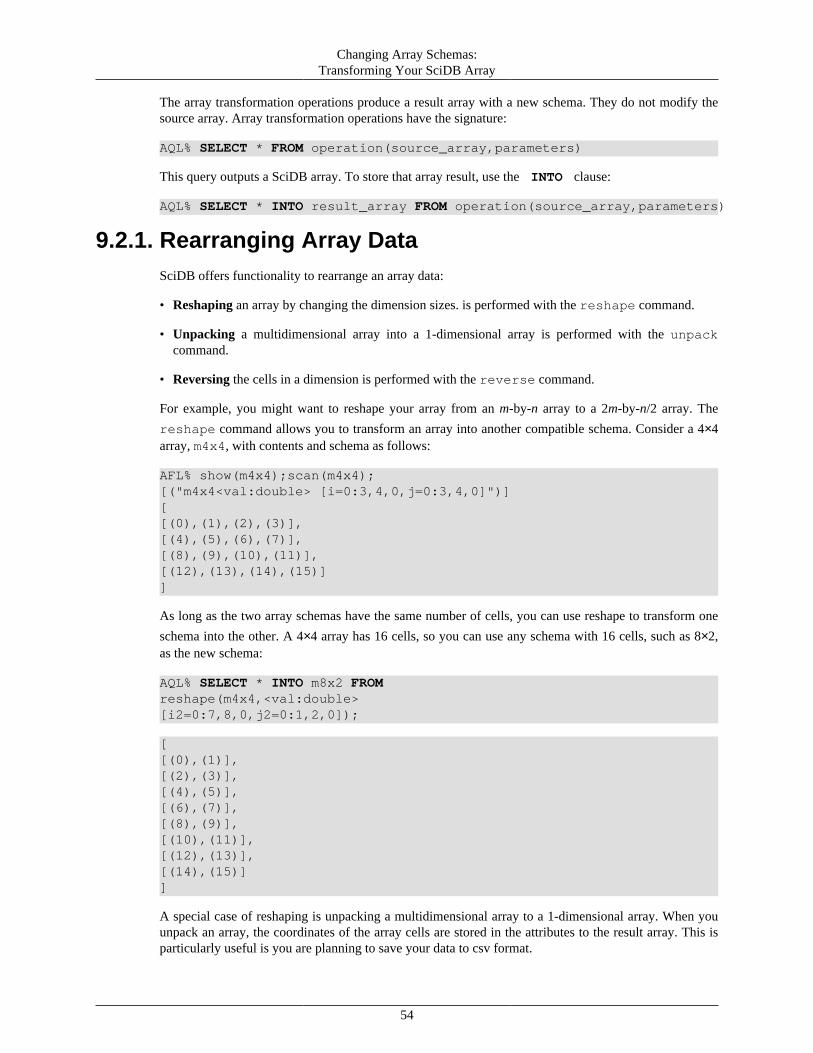
Changing Array Schemas:Transforming Your SciDB Array
54
The array transformation operations produce a result array with a new schema. They do not modify thesource array. Array transformation operations have the signature:
AQL% SELECT * FROM operation(source_array,parameters)
This query outputs a SciDB array. To store that array result, use the INTO clause:
AQL% SELECT * INTO result_array FROM operation(source_array,parameters)
9.2.1. Rearranging Array DataSciDB offers functionality to rearrange an array data:
• Reshaping an array by changing the dimension sizes. is performed with the reshape command.
• Unpacking a multidimensional array into a 1-dimensional array is performed with the unpackcommand.
• Reversing the cells in a dimension is performed with the reverse command.
For example, you might want to reshape your array from an m-by-n array to a 2m-by-n/2 array. The
reshape command allows you to transform an array into another compatible schema. Consider a 4×4array, m4x4, with contents and schema as follows:
AFL% show(m4x4);scan(m4x4);[("m4x4<val:double> [i=0:3,4,0,j=0:3,4,0]")][[(0),(1),(2),(3)],[(4),(5),(6),(7)],[(8),(9),(10),(11)],[(12),(13),(14),(15)]]
As long as the two array schemas have the same number of cells, you can use reshape to transform one
schema into the other. A 4×4 array has 16 cells, so you can use any schema with 16 cells, such as 8×2,as the new schema:
AQL% SELECT * INTO m8x2 FROM reshape(m4x4,<val:double>[i2=0:7,8,0,j2=0:1,2,0]);
[[(0),(1)],[(2),(3)],[(4),(5)],[(6),(7)],[(8),(9)],[(10),(11)],[(12),(13)],[(14),(15)]]
A special case of reshaping is unpacking a multidimensional array to a 1-dimensional array. When youunpack an array, the coordinates of the array cells are stored in the attributes to the result array. This isparticularly useful is you are planning to save your data to csv format.

Changing Array Schemas:Transforming Your SciDB Array
55
The unpack command takes the second and higher dimensions of an array and transforms them intoattributes along the first dimension. The result array consists of the dimension values of the input arraywith the attribute values from the corresponding cells appended. So, an attribute value val that was inrow 1, column 3 of a 2-dimensional array will be transformed into a cell with attribute values 1,3,val.For example, a 2-dimensional, 1-attribute array will output a 1-dimensional, 3-attribute array as follows:
AQL% SELECT * FROM show(m3x3);
[("m3x3<val:double> [i=0:2,3,0,j=0:2,3,0]")]
AQL% SELECT * INTO m1 FROM unpack(m3x3,k);
[(0,0,0),(0,1,1),(0,2,2),(1,0,3),(1,1,4),(1,2,5),(2,0,6),(2,1,7),(2,2,8),(0,0,0),(0,0,0),(0,0,0)]
AQL% SELECT * FROM show(m1);
[("m1<i:int64,j:int64,val:double>[val1=0:15,4,0]")]
You can reverse the ordering of the data in each dimension of an array with the reverse command:
AFL% show(m3x3);scan(m3x3);
[("m3x3<val:double> [i=0:2,3,0,j=0:2,3,0]")][[(0),(1),(2)],[(3),(4),(5)],[(6),(7),(8)]]
AQL% SELECT * FROM reverse(m3x3);
[[(8),(7),(6)],[(5),(4),(3)],[(2),(1),(0)]]
9.2.2. Reduce an ArrayOne common array task is selecting subsets of an array. SciDB allows you to reduce an array to contiguoussubsets of the array cells or noncontiguous subsets of the array's cells.
• A subarray is a contiguous block of cells from an array. This action is performed by the subarraycommand.
• An array slice is a subset of the array defined by planes of the array. This action is performed by theslice command.

Changing Array Schemas:Transforming Your SciDB Array
56
• A dimension can be winnowed or thinned by selecting data at intervals along its entirety. This actionis performed by the thin command.
You can select part of an existing array into another array with the subarray command. For example,you can select a 2-by-2 array of the last two values from each dimension of the array m4x4 with thefollowing subarray command:
AFL% show(m4x4);scan(m4x4);[("m4x4<val:double> [i=0:3,4,0,j=0:3,4,0]")]
[[(0),(1),(2),(3)],[(4),(5),(6),(7)],[(8),(9),(10),(11)],[(12),(13),(14),(15)]]
AQL% SELECT * FROM subarray(m4x4,2,2,3,3);
[[(10),(11)],[(14),(15)]]
If you have a 3-dimensional array, you might want to select just a flat 2-dimensional slice, as like thecross-hatched section of this image:
For example, you can select the data in a horizontal slice in the middle of a 3-dimensional array m3x3x3by using the slice command and specifying the value for dimension k:
AFL% show(m3x3x3);scan(m3x3x3);[("m3x3x3<val:double>[i=0:2,3,0,j=0:2,3,0,k=0:2,3,0]")]
[[[(0),(1),(2)],[(4),(5),(6)],[(8),(9),(10)]],

Changing Array Schemas:Transforming Your SciDB Array
57
[[(7),(8),(9)],[(11),(12),(13)],[(15),(16),(17)]],[[(14),(15),(16)],[(18),(19),(20)],[(22),(23),(24)]]]
AFL% slice(m3x3x3,k,1);
[[(1),(5),(9)],[(8),(12),(16)],[(15),(19),(23)]]
You may want to sample data uniformly across an entire dimension. The thin command selects elementsfrom given array dimensions at defined intervals. For example, you can select every other element fromevery other row:
AFL% show(m4x4);scan(m4x4);[("m4x4<val:double> [i=0:3,4,0,j=0:3,4,0]")]
[[(0),(1),(2),(3)],[(4),(5),(6),(7)],[(8),(9),(10),(11)],[(12),(13),(14),(15)]]
AQL% SELECT * FROM thin(m4x4,1,2,0,2);
[[(4),(6)],[(12),(14)]]
9.3. Changing Array AttributesAn array's attributes contain the data stored in the array. You can transform attributes by
• Changing the name of the attribute.
• Adding an attribute.
• Changing the order of attributes in a cell.
• Deleting an attribute.
You can change the name of an attribute with the attribute_rename command:
AQL% SELECT * INTO m3x3_new FROM attribute_rename(m3x3,val,val2);

Changing Array Schemas:Transforming Your SciDB Array
58
[[(0),(1),(2)],[(3),(4),(5)],[(6),(7),(8)]]
AQL% SELECT * FROM show(m3x3_new);
[("m3x3_new<val2:double> [i=0:2,3,0,j=0:2,3,0]")]
You can add attributes to an existing array with the apply command:
AQL% SELECT * INTO m3x3_new_attr FROM apply(m3x3,val2,val+10,val3,pow(val,2));
[[(0,10,0),(1,11,1),(2,12,4)],[(3,13,9),(4,14,16),(5,15,25)],[(6,16,36),(7,17,49),(8,18,64)]]
AQL% SELECT * FROM show(m3x3_new_attr);
[("m3x3_new_attr<val:double,val2:double,val3:double> [i=0:2,3,0,j=0:2,3,0]")]
You can select a subset of an array's attributes and return them in any order with the project command.
AQL% SELECT * FROM project(m3x3_new_attr,val3,val2);
[[(0,10),(1,11),(4,12)],[(9,13),(16,14),(25,15)],[(36,16),(49,17),(64,18)]]
9.4. Changing Array Dimensions
9.4.1. Changing Chunk SizeIf you have created an array with a particular chunk size and then later find that you need a different chunksize, you can use the repart command to change the chunk size. For example, suppose you have anarray that is 1000-by-1000 with chunk size 100 in each dimension:
AQL% SELECT * FROM show(chunks);
[("chunks<val1:double,val2:double>[i=0:999,100,0,j=0:999,100,0]")]
You can repartition the chunks to be 10 along one dimension and 1000 in the other:
AQL% SELECT * INTO chunks_part

Changing Array Schemas:Transforming Your SciDB Array
59
FROM repart(chunks,<val1:double,val2:double> [i=0:999,10,0,j=0:999,1000,0]);
AQL% SELECT * FROM show(chunks_part);
[("chunks_part<val1:double,val2:double> [i=0:999,10,0,j=0:999,1000,0]")]
Repartitioning is also important if you want the change the chunk overlap to speed up nearest-neighboror window aggregate queries.
AQL% SELECT * INTO chunks_overlap FROM repart(chunks,<val1:double,val2:double> [i=0:999,100,10,j=0:999,100,10]);
9.4.2. Appending a DimensionYou may need to append dimensions to existing arrays, particularly when you want to do more complicatedtransformations to your array. This example demonstrates how you can take slices from an existing arrayand then reassemble them into a array with a different schema. Consider the following 2-dimensional array:
AFL% show(Dsp);scan(Dsp);
[("Dsp<val:double>[d(string)=5,5,0,t(string)=5,5,0]")]
[[(0.01),(30.36),(111.21),(242.56),(424.41)],[(2.04),(42.49),(133.44),(274.89),(466.84)],[(6.09),(56.64),(157.69),(309.24),(511.29)],[(12.16),(72.81),(183.96),(345.61),(557.76)],[(20.25),(91),(212.25),(384),(606.25)]]
Suppose you want to examine a sample plane from each dimension of the array. You can use the slicecommand to select array slices from array Dsp:
AQL% SELECT * INTO Dsp_slice_0 FROM slice(Dsp,s,'device-0');
AQL% SELECT * INTO Dsp_slice_1 FROM slice(Dsp,s,'device-1');
AQL% SELECT * INTO Dsp_slice_2 FROM slice(Dsp,s,'device-2');
The slices are 1-dimensional.
AQL% SELECT * FROM show(Dsp_slice_0);
[("Dsp_slice_0<val:double>[t(string)=5,5,0]")]
Concatenating these slices will create a 1-d array:
AQL% SELECT * INTO Dsp_1d FROM concat(Dsp_slice_0,Dsp_slice_2);AQL% SELECT * FROM show(Dsp_1d);

Changing Array Schemas:Transforming Your SciDB Array
60
[("Dsp_1d<val:double,empty_indicator:indicator> [t=0:9,5,0]")]
To concatenate these arrays into a 2-dimensional array, you need to add a dimension to both. The adddimcommand will add a stub dimension to the array to increase its dimensionality.
AQL% SELECT * INTO Dsp_new FROM concat(adddim(Dsp_slice_0, s), adddim(Dsp_slice_2, d));AQL% SELECT * FROM show(Dsp_new);
[("Dsp_new<val:double,empty_indicator:indicator>[d=0:1,1,0,t(string)=5,5,0]")]

61
Chapter 10. SciDB AggregateReference
This chapter lists SciDB aggregates. Aggregates take as input a set of 1 or more values and return a scalarvalue. SciDB aggregates have the syntax aggregate_call_N where an aggregate call is one of the following:
• aggregate_name(attribute_name)
• aggregate_name(expression)
Note: the aggregate_name(expression) syntax exists only in AQL.
Aggregate calls can occur in AQL and AFL statements as follows:
AQL syntaxes
SELECT aggregate_call_1[,aggregate_call_2,...,aggregate_call_N] FROM array;
SELECT aggregate_call_1[,aggregate_call_2,...,aggregate_call_N] FROM array GROUP BY dimension1[,dimension2];
SELECT aggregate_call_1[,aggregate_call_2,...,aggregate_call_N] FROM array WHERE expression;
SELECT aggregate_call_1[,aggregate_call_2,...,aggregate_call_N] FROM array REGRID dimension_1, dimension_2,...
SELECT aggregate_call_1[,aggregate_call_2,...,aggregate_call_N] FROM array WINDOW window_dim_1, window_dim_2,...
AFL syntaxes
aggregate(array, aggregate_call_1[, aggregate_call_2,... aggregate_call_N][,dimension_1, dimension_2,...])
window(array,grid_1,grid_2,...,grid_N,aggregate_call_1 [,aggregate_call_2,...,aggregate_call_N]);
regrid(array,grid_1,grid_2,...,grid_N,aggregate_call_1[,aggregate_call_2,...,aggregate_call_N]);

SciDB Aggregate Reference
62
Nameavg — Average (mean) aggregate
SynopsisAQL% SELECT avg(attribute) FROM array;
AFL% aggregate(array,avg(attribute)[,dimension_1,dimension_2,...]
SummaryThe avg aggregate takes a set of scalar values from an array attribute and returns the average of thosevalues.
The average of an empty set is NULL. avg of a set that contains only NULL values is also NULL. If theset contains NULL and NOT NULL values, the avg result is an average of the NOT NULL values only.
Example
This example finds the average of every column of a 3×3 matrix.
1. Create a matrix m3x3:
CREATE ARRAY m3x3<val:double>[i=0:2,3,0,j=0:2,3,0];
2. Put values of 0–8 into m3x3:
store(build(m3x3,i*3+j),m3x3);
[[(0),(1),(2)],[(3),(4),(5)],[(6),(7),(8)]]
3. Find the average of every column of m3x3:
aggregate(m3x3,val,j)
This query returns:
[(3),(4),(5)]

SciDB Aggregate Reference
63
Namecount — Count nonempty elements aggregate
SynopsisAQL% SELECT count(attribute) FROM array;
AFL% aggregate(array,count(attribute)[,dimension_1,dimension_2,...)]
SummaryThe count aggregate counts nonempty elements of an array's attributes. count(attr1), only counts the cellsthat have values that are NOT NULL. count(*), counts all of the cells present (both NULL and NOTNULL).
Example
This example finds the number of nonempty cells in a 3×3 matrix.
1. Create a matrix m3x3:
CREATE ARRAY m3x3<val:double>[i=0:2,3,0,j=0:2,3,0];
2. Put values 1 along the diagonal of m3x3 and leave the remaining cells empty:
store(build_sparse(m3x3,i=j,1),m3x3);
3. Find the number of nonempty cells in the array:
aggregate(m3x3,count(val));
This query returns:
[(6)]

SciDB Aggregate Reference
64
Namemax — Maximum value aggregate
SynopsisAQL% SELECT max(attribute) FROM array;
AFL% aggregate(array,max(attribute)[,dimension_1,dimension_2,...]
SummaryThe max aggregate takes a set of scalar values from an array attribute and returns the maximum value.
The maximum value of an empty set is NULL. max of a set that contains only NULL values is also NULL.If the set contains NULL and NOT NULL values, the max aggregate considers only NOT NULL values.
Example
This example finds the maximum of every column of a 3×3 matrix.
1. Create a matrix m3x3:
CREATE ARRAY m3x3<val:double>[i=0:2,3,0,j=0:2,3,0];
2. Put values of 0–8 into m3x3:
store(build(m3x3,i*3+j),m3x3);
[[(0),(1),(2)],[(3),(4),(5)],[(6),(7),(8)]]
3. Find the maximum value of each column:
aggregate(m3x3,max(val),j);
This query returns:
[(6),(7),(8)]

SciDB Aggregate Reference
65
Namemin — Minimum value aggregate
SynopsisAQL% SELECT min(attribute) FROM array;
AFL% aggregate(array,min(attribute)[,dimension_1,dimension_2,...]
SummaryThe min aggregate takes a set of scalar values from an array attribute and returns the minimum value.
The minimum value of an empty set is NULL. min of a set that contains only NULL values is also NULL.If the set contains NULL and NOT NULL values, the min aggregate considers only NOT NULL values.
Example
This example finds the minimum of every column of a 3×3 matrix.
1. Create a matrix m3x3:
CREATE ARRAY m3x3<val:double>[i=0:2,3,0,j=0:2,3,0];
2. Put values of 0–8 into m3x3:
store(build(m3x3,i*3+j),m3x3);
[[(0),(1),(2)],[(3),(4),(5)],[(6),(7),(8)]]
3. Find the minimum value of every column of m3x3:
aggregate(m3x3,min(val),j);
This query returns:
[(0),(1),(2)]

SciDB Aggregate Reference
66
Namestdev — Standard deviation aggregate
SynopsisAQL% SELECT stdev(attribute) FROM array;
AFL% aggregate(array,stdev(attribute)[,dimension_1,dimension_2,...]
SummaryThe stdev aggregate takes a set of scalar values from an array attribute and returns the standard deviationof those values.
The standard deviation of an empty set is NULL. The standard deviation of a set that contains only NULLvalues is also NULL. If the set contains NULL and NOT NULL values, the stdev aggregate considersonly NOT NULL values.
Example
This example finds the standard deviation of every column of a 3×3 matrix.
1. Create a matrix m3x3:
CREATE ARRAY m3x3<val:double>[i=0:2,3,0,j=0:2,3,0];
2. Put random values between 1 and 9 into m3x3:
store(build(m3x3,random()%10/1.0),m3x3);
This query outputs:
[[(2),(8),(0)],[(5),(2),(6)],[(2),(0),(2)]]
3. Find the standard deviation of every column of m3x3:
aggregate(m3x3,stdev(val),j);
This query returns:
[(1.73205),(4.16333),(3.05505)]

SciDB Aggregate Reference
67
Namesum — Sum aggregate
SynopsisAQL% SELECT sum(attribute) FROM array;
AFL% aggregate(array,sum(attribute)[,dimension_1,dimension_2,...]
SummaryThe sum aggregate calculates the cumulative sum of a group of values.
The sum of an empty set is 0. The standard deviation of a set that contains only NULL values is also 0. Ifthe set contains NULL and NOT NULL values, the result is the sum of all the NOT NULL values.
Example
This example finds the sum of every column of a 3×3 matrix.
1. Create a matrix m3x3:
CREATE ARRAY m3x3<val:double>[i=0:2,3,0,j=0:2,3,0];
2. Put values of 0–8 into m3x3:
store(build(m3x3,i*3+j),m3x3);
[[(0),(1),(2)],[(3),(4),(5)],[(6),(7),(8)]]
3. Find the sum of each column in m3x3:
aggregate(m3x3,sum(val),j)
This query returns:
[(9),(12),(15)]

SciDB Aggregate Reference
68
Namevar — Variance aggregate
SynopsisAQL% SELECT var(attribute) FROM array;
AFL% aggregate(array,var(attribute)[,dimension_1,dimension_2,...]
SummaryThe var aggregate returns the variance of a set of values.
The variance of an empty set is NULL. The variance of a set that contains only NULL values is also NULL.If the set contains NULL and NOT NULL values, the var aggregate considers only NOT NULL values.
Example
This example finds the variance of every column of a 3×3 matrix.
1. Create a matrix m3x3:
CREATE ARRAY m3x3<val:double>[i=0:2,3,0,j=0:2,3,0];
2. Put random values between 1 and 9 into m3x3:
store(build(m3x3,random()%10/1.0),m3x3);
This query returns:
[[(2),(8),(0)],[(5),(2),(6)],[(2),(0),(2)]]
3. Find the variance for each column of m3x3:
aggregate(m3x3,var(val),j)
This query returns:
[(3),(17.3333),(9.33333)]

69
Chapter 11. SciDB Function ReferenceThis chapter lists the SciDB functions that are available for use in SciDB expressions. Expressions canbe used in the following types of syntaxes:
AQL Syntax:
SELECT expression FROM array;
SELECT expression1 FROM array WHERE expression2;
AFL Syntax:
operator(array,expression);
Function Name Description Category
% Remainder Arithmetic
* Multiplication Arithmetic
+ Addition Arithmetic
- Subtraction Arithmetic
/ Division Arithmetic
< Less than Logical
<= Less than or equal Logical
<> Not equal Logical
= Equals Logical
> Greater than Logical
>= Greater than or equal Logical
abs Absolute value Arithmetic
acos Inverse (arc) cosine in radians Transcendental
and Boolean AND Logical
append_offset Change time and date by a given amount Timestamp
apply_offset Change time and date by a given amount Timestamp
asin Inverse (arc) sine in radians Transcendental
atan Inverse (arc) tangent in radians Transcendental
ceil Round to next-highest integer Arithmetic
cos Cosine (input in radians) Transcendental
exp Exponential Transcendental
first Start of string Strings
floor Round to next-lowest integer Arithmetic
get_offset Returns time offset in seconds Timestamp
high String information Strings
iif Inline IF Logical
is_nan Returns TRUE is attribute value is NaN Logical

SciDB Function Reference
70
Function Name Description Category
is_null Returns TRUE is attribute value is null Logical
last End of string String
length Get string length String
log Base-e logarithm Transcendental
log10 Base-10 logarithm Transcendental
low String query String
instanceid Return instance id Troubleshooting
not Boolean NOT Logical
now Current array version Timestamp
or Boolean OR Logical
pow Raise to a power Arithmetic
random Random number Arithmetic
regex Search for regular expression Strings
sin Sine (input in radians) Transcendental
sqrt Square root Arithmetic
strchar Convert string to char Datatype conversion
strftime Convert string to datetime Datatype conversion
strip_offset disregards OFFSET and returns result as aDATETIME
Timestamp
strlen Maximum string length Strings
substr Select substring Strings
tan Tangent (input in radians) Transcendental
togmt Switch to GMT from current time zone setting Timestamp
tznow Set time zone Timestamp

71
Chapter 12. SciDB Data TypeReference
SciDB supports the following data types. You can access this list by using list('types') at the AFLcommand line.
Data Type Default Value Description
bool false Boolean TRUE (1) or FALSE (0)
char \0 Single-character
datetime 1970-01-01 00:00:00 Date and time
datetimetz 1970-01-01 00:00:00 -00:00 Timezone
double 0 Double-precision decimal
float 0 Floating-point number
int8 0 Signed 8-bit integer
int16 0 Signed 16-bit integer
int32 0 Signed 32-bit integer
int64 0 Signed 64-bit integer
string "" Character string
uint8 0 Unsigned 8-bit integer
uint16 0 Unsigned 16-bit integer
uint32 0 Unsigned 32-bit integer
uint64 0 Unsigned 64-bit integer

72
Chapter 13. SciDB Operator ReferenceThis reference guide lists the operators available in SciDB. Operators take a SciDB array as input andreturn as SciDB array as output. Operators can be used in several ways in SciDB queries.
• Operators can be used in AQL in FROM clauses.
• Operators can be used at the AFL command line or, in some cases, nested with other AFL operators.
Operator syntaxes generally follow this pattern:
operator(array|array_expression|anonymous_schema,arguments);
The first argument to an operator is generally an array that you have previously created and stored in yourcurrent SciDB namespace. However, in many cases, the first argument may also be a SciDB operator. Theoutput of the nested operator serves as the input for the outer operator. This is called an array expression.
operator_1(operator_2(array,arguments_2),arguments_1);
Not all SciDB operators can take another operator as input. These exceptions are noted in the Synopsissection of the operator's reference page. An operator argument that is specified as array can also be anarray expression. An operator argument that is specified as named_array can only be an array that youhave previously created and stored.
In addition, some operators can take an array schema as input instead of a named array or array expression.This is called an anonymous schema.

SciDB Operator Reference
73
Nameadddim — Increase array dimensionality
SynopsisSELECT * FROM adddim(array,new_dimension);
adddim(array,new_dimension);
SummaryThe adddim operator adds a stub dimension to an array to increase its dimensionality. This is useful whenyou want to concatenate two n-dimensional arrays into an (n+1)-dimensional array.
ExampleThis example creates a 2-dimensional array from 1-dimensional arrays.
1. Create a vector of zeros:
store(build(<val:double>[i=0:4,5,0],0),vector1);
2. Create a vector of ones:
store(build(<val:double>[j=0:4,5,0],1),vector2);
3. Concatenate these vectors without increasing their dimensionality. Note that the output is 1-dimensional:
concat(vector1,vector2);
This query outputs:
[(0),(0),(0),(0),(0),(1),(1),(1),(1),(1)]
4. Use adddim to add a dimension to both vectors and then concatenate them. The result will have twodimensions:
concat(adddim(vector1,x),adddim(vector2,y));
This query outputs:
[[(0),(0),(0),(0),(0)],[(1),(1),(1),(1),(1)]]
<xi:include></xi:include>

SciDB Operator Reference
74
Nameanalyze — Analyze load file for chunk size
SynopsisSELECT * FROM analyze(array[, attribute1, attribute2, ...])
analyze(array[, attribute1, attribute2, ...]);
SummaryThe analyze operator helps you decide how to set chunk size when you are creating a SciDB array. Theanalyze() operator takes as input a source array and a list of attributes in that source array. The operatorcomputes the range of values (the maximum and minimum values), population count, and an estimate ofthe number of distinct values in the attribute (or combination of attributes).
ExampleThis example runs analyze on a 2-attribute, 1-dimensional array. The example uses the file doc/user/examples/num_data.scidb, shown here:
{0}[(1.48306e+09,1),(5.80814e+08,1),(1.51079e+09,1),(1.16154e+09,1),(1.42655e+09,1),(1.06341e+09,1),(4.9253e+08,1),(5.6065e+08,1),(1.60886e+08,2),(1.37844e+09,1),(4.08495e+08,1),(5.65393e+07,1),(1.47646e+09,1),(9.52609e+08,1),(1.8548e+09,1),(1.42396e+09,1),(1.75107e+09,1),(1.52007e+09,1),(5.4882e+08,1),(7.28928e+08,1)]
1. Create an array analyze_array with 1 unbounded dimension:
AQL% CREATE ARRAY analyze_array<val1:double,val2:double> [line=0:*,10,0];
2. Load the file num_data.scidb into analyze_array:
AQL% LOAD analyze_array FROM 'path/doc/user/examples/num_data.scidb';

SciDB Operator Reference
75
3. Analyze the array for chunk sizes:
analyze(analyze_array);
This query returns:
[("val","5.65393e+07","1.8548e+09",20,20),("val2","1","2",2,20)]
The output array contains one attribute for every attribute in the input. Each attribute of the outputcontains the attribute name, maximum value, minimum value, number of distinct elements, and totalnumber of elements.
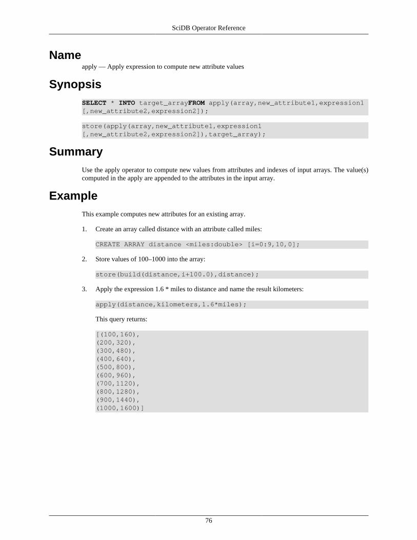
SciDB Operator Reference
76
Nameapply — Apply expression to compute new attribute values
SynopsisSELECT * INTO target_arrayFROM apply(array,new_attribute1,expression1[,new_attribute2,expression2]);
store(apply(array,new_attribute1,expression1[,new_attribute2,expression2]),target_array);
SummaryUse the apply operator to compute new values from attributes and indexes of input arrays. The value(s)computed in the apply are appended to the attributes in the input array.
ExampleThis example computes new attributes for an existing array.
1. Create an array called distance with an attribute called miles:
CREATE ARRAY distance <miles:double> [i=0:9,10,0];
2. Store values of 100–1000 into the array:
store(build(distance,i+100.0),distance);
3. Apply the expression 1.6 * miles to distance and name the result kilometers:
apply(distance,kilometers,1.6*miles);
This query returns:
[(100,160),(200,320),(300,480),(400,640),(500,800),(600,960),(700,1120),(800,1280),(900,1440),(1000,1600)]

SciDB Operator Reference
77
Nameattribute_rename — Rename an array attribute
SynopsisSELECT * FROM attribute_rename(array,old_attribute1,new_attribute1[, old_attribute2,new_attribute2]);
attribute_rename(array,old_attribute1,new_attribute1[, old_attribute2,new_attribute2]);
SummaryChanges an attribute name in an array.
Example1. Create an array called array1 with an attribute called val:
CREATE ARRAY array1 <val:double>[i];
2. Rename val to val2:
attribute_rename(array1,val,val2);

SciDB Operator Reference
78
Nameattributes — List array attributes
SynopsisSELECT * FROM attributes(named_array);
attributes(named_array);
SummaryThe attributes operator lists all the attributes of an array. The output returns the attribute name, theattribute data type, and a Boolean flag representing whether or not the attribute can be null. The argumentnamed_array must be an array that was previously created and stored in the SciDB namespace.

SciDB Operator Reference
79
Nameavg — Average (mean) value
SynopsisSELECT * FROM avg(array,attribute[,dimension1,dimension2,...]);
SummaryThe avg operator finds the average value of an array attribute.
Note
The avg operator provides the same functionality as the avg aggregate, but has a different syntax.See the avg aggregate reference page.
Example
This example finds the average value along the second dimension of a 4×4 matrix.
1. Create an array named avg_array:
CREATE ARRAY avg_array<val:double>[i=0:3,4,0,j=0:3,4,0];
2. Store values of 0–15 in avg_array:
store(build(avg_array,i*4+j),avg_array);
[[(0),(1),(2),(3)],[(4),(5),(6),(7)],[(8),(9),(10),(11)],[(12),(13),(14),(15)]]
3. Find the average value along the dimension j:
avg(avg_array,val,j);
This query outputs:
[(1.5),(5.5),(9.5),(13.5)]

SciDB Operator Reference
80
Namebernoulli — Select random array cells
SynopsisSELECT * FROM bernoulli(array,probability[, seed]);
bernoulli(array,probability[, seed]);
SummaryThe bernoulli operator evaluates each cell by generating a random number and seeing if it lies in the range(0, probability). If it does, the cell is included.
Example
This example select cells at random from a 4×4 matrix, and uses a seed value to select the same cells insuccessive trials.
1. Create an array called bernoulli_array:
CREATE ARRAY bernoulli_array<val:double>[i=0:3,4,0,j=0:3,4,0];
2. Store values of 0–15 in bernoulli_array:
store(build(bernoulli_array,i*4+j),bernoulli_array);
[[(0),(1),(2),(3)],[(4),(5),(6),(7)],[(8),(9),(10),(11)],[(12),(13),(14),(15)]]
3. Select cells at random with a probability of .5 that a cell will be included. Each successive call tobernoulli will return different results.
AFL% bernoulli(bernoulli_array,.5);
[[(),(1),(),(3)],[(4),(),(),()],[(),(9),(),(11)],[(12),(),(14),(15)]]
bernoulli(bernoulli_array,.5);
[[(),(1),(),(3)],[(),(5),(6),()],[(),(9),(),(11)],[(),(13),(14),()]]

SciDB Operator Reference
81
4. To reproduce earlier results, use a seed value. Seeds must be an integer on the interval [0, INT_MAX].
bernoulli(bernoulli_array,.5,1);
[[(),(),(2),()],[(),(),(6),(7)],[(8),(9),(),(11)],[(12),(),(),()]]
AFL% bernoulli(bernoulli_array,.5,1);
[[(),(),(2),()],[(),(),(6),(7)],[(8),(9),(),(11)],[(12),(),(),()]]

SciDB Operator Reference
82
Namebetween — Select array data from specified region
SynopsisSELECT * FROM between(array,low_coord1[,low_coord2,...],high_coord1[,high_coord2,...]);
between(array,low_coord1[,low_coord2,...],high_coord1[,high_coord2,...]);
SummaryThe between operator accepts an input array and a set of coordinates specifying a region within the array.The number of coordinate pairs in the input must be equal to the number of dimensions in the array. Theoutput is an array of the same shape as input, where all cells outside of the given region are marked empty.
ExampleThis example selects 4 elements from a 16-element array.
1. Create a 4×4 array called between_array:
CREATE ARRAY between_array <val:double>[i=0:3,4,0,j=0:3,4,0];
2. store(build(between_array,i*4+j),between_array);
[[(0),(1),(2),(3)],[(4),(5),(6),(7)],[(8),(9),(10),(11)],[(12),(13),(14),(15)]]
3. Select all values from the last two rows and last two columns from between_array:
between(between_array,2,2,3,3);
This query outputs:
[[(),(),(),()],[(),(),(),()],[(),(),(10),(11)],[(),(),(14),(15)]]

SciDB Operator Reference
83
Namebuild — Assign values to array attribute
SynopsisSELECT * INTO target_arrayFROM build(named_array|anonymous_schema,expression);
store(build(named_array|anonymous_schema,expression),target_array;
SummaryThe build operator proceeds through source_array, cell by cell, using the value of expression tocompute the value of each cell. The expression argument can be any combination of SciDB functionsapplied to scalars or SciDB array attributes.
ExampleCreate an array of all ones:
build(<val:double>[i=0:3,4,0,j=0:3,4,0],1);
Create an identity matrix:
build(<val:double>[i=0:3,4,0,j=0:3,4,0],iif(i=j,1,0));
Build an array of monotonically increasing values:
build(<val:double>[i=0:3,4,0,j=0:3,4,0],i*4+j);
To store the result from a build operator, create an array and use the store operator with the build operator.
CREATE ARRAY identity_matrix <val:double>[i=0:3,4,0,j=0:3,4,0];store(build(identity_matrix,iif(i=j,1,0)),identity_matrix);
Limitations• The build operator can only take arrays with one attribute.
• The build operator can only take arrays with bounded dimensions.

SciDB Operator Reference
84
Namebuild_sparse — Assign values to attributes of a sparse array
SynopsisSELECT * INTO target_arrayFROM build_sparse(named_array|anonymous_schema,expression,boolean_expression);
store(build_sparse(named_array|anonymous_schema,expression,boolean_expression));
SummaryThe build_sparse operator takes as input an array or anonymous schema, an expression that defines ascalar value, and an expression that defines a Boolean value. The argument named_array must bean array that was previously created and stored in the SciDB namespace. The output of build_sparsecontains an array with the same schema as the input array or anonymous schema, the value specifiedby expression wherever boolean_expression evaluates to true, and empty cells whereverboolean_expression evaluates to false.
ExampleBuild a sparse-formatted identity matrix where the cells that would be occupied by 0 are empty:
build_sparse(<val:double>[i=0:3,4,0,j=0:3,4,0],1,i=j);
This query outputs:
[[{0,0}(1),{1,1}(1),{2,2}(1),{3,3}(1)]]
Limitations• The build operator can only take arrays with one attribute.
• The build operator can only take arrays with bounded dimensions.

SciDB Operator Reference
85
Namecancel — Cancel a query
Synopsiscancel(query_id);
This operator is designed for internal use.
SummaryCancel a currently running query by query id.
The query id can be obtained from the SciDB log or via the list() command. SciDB maintains query contextinformation for each completed and in-progress query in the server. If the user issues a "ctrl-C" or abortfrom the client, the query is cancelled and its context is removed from the server.

SciDB Operator Reference
86
Namecast — Change attribute and dimension names
SynopsisSELECT * INTO target_array FROM cast(array, schema);
store(cast(array,schema),target_array);
SummaryThe cast operator allows renaming an array or any of its attributes and dimensions. A single cast invocationcan be used to rename multiple items at once (one or more attribute names and/or one or more dimensionnames). The input array and template arrays should have the same numbers and types of attributes and thesame numbers and types of dimension.
ExampleThis example changes the name of an array attribute and an array dimension. The arrays must becompatible; that is, they must have the same number of dimensions and attributes, and the attributes anddimensions must be of the same type.
1. Create an array called source with an attribute called val and a dimension called i:
CREATE ARRAY source <val:double>[i=0:9,10,0];
2. Use an anonymous schema to change the attribute name to num_val and the dimension name to x.Store the result in an array called target:
store(cast(source, <num_val:double>[x=0:9,10,0]),target);
This is useful when you are joining arrays and want to avoid naming conflicts. For example, doinga cross_join on source and target will create an array with two attributes, val and num_val, and twodimensions, i and x:
store(cross_join(source,target),new_array);show(new_array);
[("new_array<val:double,num_val:double> [i=0:9,10,0,x=0:9,10,0]")]

SciDB Operator Reference
87
Nameconcat — Concatenate two arrays
SynopsisSELECT * INTO target_array FROM concat(left_array,right_array);
store(concat(left_array,right_array),target_array);
SummaryThe concat operator concatenates two arrays with the name number of dimensions. Concatenation isperformed by the left-most dimension. All other dimensions of the input arrays must match. The left-mostdimension of both arrays must have a fixed size (not unbounded) and same chunk size and overlap. Bothinputs must have the same attributes.
Example
This example concatenates a 4×3 array and a 1×3 array.
1. Create a 4×3 array left_array containing value 1 in all cells:
create array left_array <val:double>[i=0:3,1,0,j=0:3,1,0];store(build(left_array,1),left_array);
2. Create a 1×3 array right_array containing value 0 in all cells:
create array right_array <val:double>[i=0:1,1,0,j=0:2,1,0];store(build(right_array,0),right_array);
3. Concatentate left_array and right_array and store the result in concat_array:
store(concat(left_array,right_array),concat_array);
This produces an array concat_array with contents and schema as follows:
show(concat_array);scan(concat_array);
show(concat_array);scan(concat_array);[("concat_array<val:double> [i=0:5,1,0,j=0:2,1,0]")][[(1)]];[[(1)]];[[(1)]];[[(1)]];[[(1)]];[[(1)]];[[(1)]];[[(1)]];[[(1)]];[[(1)]];[[(1)]];[[(1)]];[[(0)]];[[(0)]];[[(0)]];[[(0)]];[[(0)]];[[(0)]]

SciDB Operator Reference
88
Namecount — Count nonempty cells
SynopsisSELECT * FROM count(array);
SummaryThe count operator counts nonempty cells of the input array. When dimensions are provided they are usedto do a group-by and a count per resulting group is returned.
Note
The count operator provides the same functionality as the count aggregate. See the countaggregate page.
Example
This example finds the element count value along the second dimension of a 4×4 array where some cellsare empty.
1. Create an array named source_array:
CREATE ARRAY source_array<val:double>[i=0:3,4,0,j=0:3,4,0];
2. Store values of 0–15 in source_array:
store(build(source_array,i*4+j),source_array);
[[(0),(1),(2),(3)],[(4),(5),(6),(7)],[(8),(9),(10),(11)],[(12),(13),(14),(15)]]
3. Use between to create some empty cells in source_array and store the result in count_array:
store(between(source_array,1,1,1,2),count_array);
[[(),(),(),()],[(),(5),(6),()],[(),(),(),()],[(),(),(),()]]
4. Find the count of nonempty elements in count_array:
count(count_array);
This query outputs:

SciDB Operator Reference
89
[(2)]
5. Count the nonempty elements along the dimensions of count_array:
count(count_array,i);
[(0),(2),(0),(0)]
count(count_array,j);
[(0),(1),(1),(0)]

SciDB Operator Reference
90
Namecross — Cross-product join
SynopsisSELECT * INTO target_array FROM cross(left_array,right_array);
cross(left_array,right_array);
SummaryCalculates the full cross product join of two arrays, for example A (m-dimensional) and B (n-dimensional),such that the result is an m+n dimensional-array in which each cell is computed as the concatenation ofthe attribute lists from corresponding cells in arrays A and B. For example, consider a 2-dimensional arrayA with dimensions i, j, and a 1-dimensional array B with dimension k. The cell at coordinate position {i,j, k} of the output is computed as the concatenation of cells {i, j} of A with cell at coordinate {k} of B.
Example
This example returns the cross-join of a 3×3 array with a vector of length 2.
1. Create a 3×3 array m3x3:
CREATE ARRAY m3x3<val:double>[i=0:2,3,0,j=0:2,3,0];
2. Put values of 0–8 into m3x3:
store(build(m3x3,i*3+j),m3x3);
3. Create a vector of length 2 containing values 101 and 102:
store(build(<val:double>[i=0:1,1,0],i+101),vector);
4. Find the cross of m3x3 and vector:
store(cross(m3x3,vector),cross_array);
This query returns:
[[[(0,101)],[(1,101)],[(2,101)]],[[(3,101)],[(4,101)],[(5,101)]],[[(6,101)],[(7,101)],[(8,101)]]];
[[[(0,102)],[(1,102)],[(2,102)]],[[(3,102)],[(4,102)],[(5,102)]],[[(6,102)],[(7,102)],[(8,102)]]]
The array cross_array has schema:
show(cross_array);
[("cross_array<val:double,val_2:double>[i=0:2,3,0,j=0:2,3,0,i_2=0:1,1,0]")]
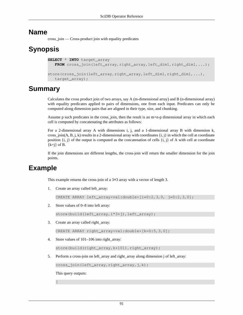
SciDB Operator Reference
91
Namecross_join — Cross-product join with equality predicates
SynopsisSELECT * INTO target_array FROM cross_join(left_array,right_array,left_dim1,right_dim1,...);
store(cross_join(left_array,right_array,left_dim1,right_dim1,...), target_array);
SummaryCalculates the cross product join of two arrays, say A (m-dimensional array) and B (n-dimensional array)with equality predicates applied to pairs of dimensions, one from each input. Predicates can only becomputed along dimension pairs that are aligned in their type, size, and chunking.
Assume p such predicates in the cross_join, then the result is an m+n-p dimensional array in which eachcell is computed by concatenating the attributes as follows:
For a 2-dimensional array A with dimensions i, j, and a 1-dimensional array B with dimension k,cross_join(A, B, j, k) results in a 2-dimensional array with coordinates {i, j} in which the cell at coordinateposition {i, j} of the output is computed as the concatenation of cells {i, j} of A with cell at coordinate{k=j} of B.
If the join dimensions are different lengths, the cross-join will return the smaller dimension for the joinpoints.
Example
This example returns the cross-join of a 3×3 array with a vector of length 3.
1. Create an array called left_array:
CREATE ARRAY left_array<val:double>[i=0:2,3,0, j=0:2,3,0];
2. Store values of 0–8 into left array:
store(build(left_array,i*3+j),left_array);
3. Create an array called right_array:
CREATE ARRAY right_array<val:double>[k=0:5,3,0];
4. Store values of 101–106 into right_array:
store(build(right_array,k+101),right_array);
5. Perform a cross-join on left_array and right_array along dimension j of left_array:
cross_join(left_array,right_array,j,k);
This query outputs:
[

SciDB Operator Reference
92
[(0,101),(1,102),(2,103)],[(3,101),(4,102),(5,103)],[(6,101),(7,102),(8,103)]]

SciDB Operator Reference
93
Namedeldim — Reduce array dimensionality
SynopsisSELECT * FROM deldim(array);
deldim(array);
SummaryThe deldim operator deletes the left-most dimension from the array. Deleted dimension must have size = 1.

SciDB Operator Reference
94
Namedimensions — List array dimensions
SynopsisSELECT * FROM dimensions(named_array);
dimensions(named_array);
SummaryThe argument to the dimensions operator is the name of the array. It returns an array with the followingattributes: dimension-name, dimension start-index, dimension-length, chunk size, chunk overlap, low-boundary-index, high-boundary-index, datatype. The argument named_array must be an array that waspreviously created and stored in the SciDB namespace.
ExampleThis example creates an array with one unbounded dimension and one string-type dimension:
CREATE ARRAY unbound_string_dim<val:double>[i=0:*,10,0,j(string)=10,10,0];dimensions(unbound_string_dim);
This code outputs:
[("i",0,4611686018427387903,10,0,4611686018427387903,-4611686018427387903,"int64"),("j",0,10,10,0,4611686018427387903,-4611686018427387903,"string")]

SciDB Operator Reference
95
Namediskinfo — Internal debugging: Check disk capacity
Synopsisdiskinfo()
This operator is designed for internal use.
SummaryGet information about storage space. Returns an array with the following attributes:
• used
• available
• clusterSize
• nFreeClusters
• nSegments
SciDB Operator Reference
96
Nameecho — Print string
Synopsisecho(string)
This operator is designed for internal use.
SummaryAccepts a string and returns a single-element array containing the string.

SciDB Operator Reference
97
Nameexplain_logical, explain_physical — Show query plan
Synopsisexplain_logical( query: string, language: string )explain_physical( query: string, language: string )
This operator is designed for internal use.
SummaryThe operators explain_logical and explain_physical can be used to emit a human-readable plan string fora particular query without running the query itself. SciDB first constructs a logical plan, optimizes it andthen translates it into a physical plan.
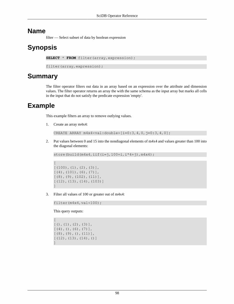
SciDB Operator Reference
98
Namefilter — Select subset of data by boolean expression
SynopsisSELECT * FROM filter(array,expression);
filter(array,expression);
SummaryThe filter operator filters out data in an array based on an expression over the attribute and dimensionvalues. The filter operator returns an array the with the same schema as the input array but marks all cellsin the input that do not satisfy the predicate expression 'empty'.
ExampleThis example filters an array to remove outlying values.
1. Create an array m4x4:
CREATE ARRAY m4x4<val:double>[i=0:3,4,0,j=0:3,4,0];
2. Put values between 0 and 15 into the nondiagonal elements of m4x4 and values greater than 100 intothe diagonal elements:
store(build(m4x4,iif(i=j,100+i,i*4+j),m4x4);
[[(100),(1),(2),(3)],[(4),(101),(6),(7)],[(8),(9),(102),(11)],[(12),(13),(14),(103)]]
3. Filter all values of 100 or greater out of m4x4:
filter(m4x4,val<100);
This query outputs:
[[(),(1),(2),(3)],[(4),(),(6),(7)],[(8),(9),(),(11)],[(12),(13),(14),()]]

SciDB Operator Reference
99
Namehelp — Operator signature
SynopsisSELECT * FROM help(operator_name);
help(operator_name);
SummaryAccepts an operator name and returns an array containing a human-readable signature for that operator.
ExampleThis example returns the signature of the multiply operator.
help('multiply');

SciDB Operator Reference
100
Nameinput — Read a system file
SynopsisSELECT * INTO target_array FROM input(named_array|anonymous_schema,filename[,instance]);
store(input(target_array|anonymous_schema,filename[,instance]), target_array);
SummaryInput works exactly the same way as load, except it does NOT store the data unless the INTO clause or theAFL store operator is present. The instance_id argument allows you to select which SciDB instance youwant to input into. To see a list of SciDB instances running on your system, type scidb.py statushostname at the Unix command-line.
ExampleThis example reads a csv file from the examples directory.
input(m4x4,'path/trunk/doc/user/examples/m4x4_missing.txt);
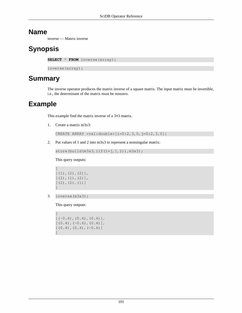
SciDB Operator Reference
101
Nameinverse — Matrix inverse
SynopsisSELECT * FROM inverse(array);
inverse(array);
SummaryThe inverse operator produces the matrix inverse of a square matrix. The input matrix must be invertible,i.e., the determinant of the matrix must be nonzero.
Example
This example find the matrix inverse of a 3×3 matrix.
1. Create a matrix m3x3:
CREATE ARRAY <val:double>[i=0:2,3,0,j=0:2,3,0];
2. Put values of 1 and 2 into m3x3 to represent a nonsingular matrix:
store(build(m3x3,iif(i=j,1,2)),m3x3);
This query outputs:
[[(1),(2),(2)],[(2),(1),(2)],[(2),(2),(1)]]
3. inverse(m3x3);
This query outputs:
[[(-0.6),(0.4),(0.4)],[(0.4),(-0.6),(0.4)],[(0.4),(0.4),(-0.6)]]

SciDB Operator Reference
102
Namejoin — Join two arrays
SynopsisSELECT * INTO target_array FROM join(left_array,right_array);
store(join(left_array,right_array),target_array);
SummaryJoin combines the attributes of two input arrays at matching dimension values. The two arrays must havethe same dimension start coordinates, the same chunk size, and the same chunk overlap. The join resulthas the same dimension names as the first input. If the the left-hand and right-hand arrays do not have thesame dimension size, join will return an array with the same dimensions as the smaller input array. If acell in either the left or right array is empty, the corresponding cell in the result is also empty.
ExampleThis example joins two arrays with different dimension lengths.
1. Create a 3×3 array left_array containing value 1 in all cells:
create array left_array <val:double>[i=0:2,3,0,j=0:2,3,0];store(build(left_array,1),left_array);
2. Create a 3×6 array right_array containing value 0 in all cells:
create array right_array <val:double>[i=0:2,3,0,j=0:5,3,0];store(build(right_array,0),right_array);
3. Join left_array and right_array:
store(join(left_array,right_array),result_array);
This produces an array result_array with contents and schema as follows:
show(result_array);scan(result_array);
[("result_array<val:double,val_2:double> [i=0:2,3,0,j=0:2,3,0]")][[(1,0),(1,0),(1,0)],[(1,0),(1,0),(1,0)],[(1,0),(1,0),(1,0)]]

SciDB Operator Reference
103
Namelist — List contents of SciDB namespace
SynopsisSELECT * FROM list(element)
list(element)
SummaryThe list operator allows you to get a list of elements in the current SciDB instance. The input is one ofthe following strings:
aggregates Show all operators that take as input a SciDB arrayand return a scalar.
arrays Show all functions. Each function will be listed withits available dataypes and the library in functionswhich it resides.
functions Show all libraries that are loaded in the currentSciDB instance.
instances Show all SciDB instances. Each instance will belisted with its port, id number, and time-and-datestamps for when it came online.
libraries Show all libraries that are loaded in the currentSciDB session.
operators Show all operators and the libraries in which theyreside.
types Show all the dataypes the SciDB supports.
queries Show all active queries. Each active query will havean id, a time and date when it was queries initiated,an error code, whether it generated any errors, anda status (boolean flag where TRUE means that thequery is idle).

SciDB Operator Reference
104
Nameload_library — Load a plugin
Synopsisload_library(library_name);
SummaryLoad a SciDB plugin. The act of loading a plugin shared library first registers the library in the SciDBsystem catalogs. Then it opens and examines the shared library to store its contents with SciDB's internalextension management subsystem. Shared library module which are registered with the SciDB instancewill be loaded at system start time.
Exampleload_library('librational')

SciDB Operator Reference
105
Namelookup — Select array cells by dimension index
SynopsisSELECT * FROM lookup(pattern_array,source_array);
lookup(pattern_array,source_array);
SummaryLookup maps elements from the second array using the attributes of the first array as coordinates into thesecond array. The result array has the same shape as first array and the same attributes as second array.
ExampleThis example selects a row from a 2-dimensional array.
1. Create an vector of ones called indices1:
store(build(<val1:double>[i=0:3,4,0],1),indices1);
[(1),(1),(1),(1)]
2. Create a vector with values between 0 and 3 called indices2:
store(build(<val1:double>[i=0:3,4,0],i),indices2);
[(0),(1),(2),(3)]
3. Join indices1 and indices2 into a two-attribute array called pattern_array:
store(join(indices1,indices2),pattern_array);
[(1,0),(1,1),(1,2),(1,3)]
4. Create a 2-dimensional array called source_array with values between 100 and 115:
store(build(<val:double>[i=0:3,4,0,j=0:3,4,0],i*4+j+100) ,source_array);
[[(100),(101),(102),(103)],[(104),(105),(106),(107)],[(108),(109),(110),(111)],[(112),(113),(114),(115)]]
5. Use lookup to use the dimension coordinates array pattern_array to return the second row ofsource_array:
lookup(pattern_array,source_array);
This query outputs:

SciDB Operator Reference
106
[(104),(105),(106),(107)]

SciDB Operator Reference
107
Namemax — Select maximum value
SynopsisSELECT * FROM max(array,attribute[,dimension1,dimension2,...])
SummaryThe max operator calculates the maximum of the specified attribute in the array. Result is an array withsingle element containing maximum of specified attribute.
Note
The max operator provides the same functionality as the max aggregate. See the max aggregatereference page for more information.
ExampleThis example find the maximum value of each row of a 2-dimensional array.
1. Create a 1-attribute, 2-dimensional array called m3x3:
CREATE ARRAY m3x3 <val:double>[i=0:2,3,0,j=0:2,3,0];
2. Store values of 0–8 in m3x3:
store(build(m3x3,i*3+j),m3x3);
[[(0),(1),(2)],[(3),(4),(5)],[(6),(7),(8)]]
3. Select the maximum value of each row of m3x3:
max(m3x3,val,i);
This query returns:
[(2),(5),(8)]

SciDB Operator Reference
108
Namemerge — Merge two arrays
SynopsisSELECT * INTO target_array FROM merge(left_array,right_array);
store(merge(left_array,right_array),target_array);
SummaryMerge combines elements from the input array the following way: for each cell in the two inputs, if thecell of first (left) array is not empty, then the attributes from that cell are selected and placed in the output.If the cell in the first array is marked as empty, then the attributes of the corresponding cell in the secondarray are taken. If the cell is empty in both input arrays, the output's cell is set to empty.
The two input arrays should have the same attribute list, number of dimensions, and dimension start index.If the dimensions are not the same size, merge will return an output array the same size as the larger inputarray.
ExampleThis example merges two sparse arrays.
1. Create a sparse array left_array and store value 1 in the first row:
CREATE ARRAY left_array <val:double>[i=0:2,3,0,j=0:5,3,0];store(build_sparse(left_array,1,i=0),left_array);
This query outputs:
[[{0,0}(1),{0,1}(1),{0,2}(1)]];[[{0,3}(1),{0,4}(1),{0,5}(1)]]
2. Create a sparse identity matrix called right_array
CREATE ARRAY right_array <val:double>[i=0:2,3,0,j=0:2,3,0];store(build_sparse(right_array,1,i=j),right_array);
This query outputs:
[[{0,0}(1),{1,1}(1),{2,2}(1)]]
3. Merge left_array and right_array:
merge(left_array,right_array);
This query outputs:
[[{0,0}(1),{0,1}(1),{0,2}(1),{1,1}(1),{2,2}(1)]];[[{0,3}(1),{0,4}(1),{0,5}(1)]]

SciDB Operator Reference
109
Namemin — Select minimum value
SynopsisSELECT * FROM min(array,attribute[,dimension_1,dimension_2,...]);
SummaryThe min operator selects the minimum value from an array attribute.
Note
The min operator provides the same functionality as the min aggregate. See the min aggregatereference page for more information.
ExampleThis example finds the minimum value of each row of a 2-dimensional array.
1. Create a 1-attribute, 2-dimensional array called m3x3:
CREATE ARRAY m3x3 <val:double>[i=0:2,3,0,j=0:2,3,0];
2. Store values of 0–8 in m3x3:
store(build(m3x3,i*3+j),m3x3);
[[(0),(1),(2)],[(3),(4),(5)],[(6),(7),(8)]]
3. Select the minimum value of each row of m3x3:
max(m3x3,val,i);
This query returns:
[(0),(3),(6)]

SciDB Operator Reference
110
Namemultiply — Matrix multiplication
SynopsisSELECT * FROM multiply(left_array,right_array);
multiply(left_array,right_array);
SummaryThe multiply operator performs matrix multiplication on two input matrices and returns a result matrix.
Both inputs must be compatible for the multiply operation, and both must have a single attribute. To becompatible, two matrices must have the same size of 'inner' dimension and same chunk size along thatdimension.
Example
This example multiplies a 3×2 array and a 2×3 array.
1. Create a 3×2 array lhs:
store(build(<val:double>[i=0:2,3,0,j=0:1,2,0],(i+1)*3+j),lhs);
This query outputs:
[[(3),(4)],[(6),(7)],[(9),(10)]]
2. Create a 2×3 array rhs:
store(build(<val:double>[i=0:1,2,0,j=0:2,3,0],(i+1)*3-j),rhs);
[[(3),(2),(1)],[(6),(5),(4)]]
3. Multiply lhs and rhs.
multiply(lhs,rhs)
This query returns:
[[(33),(26),(19)],[(60),(47),(34)],[(87),(68),(49)]]

SciDB Operator Reference
111
Namenormalize — Divide each element of a 1-attribute vector by the square root of the sum of squares of theelements
SynopsisSELECT * FROM normalize(array);
normalize(array);
SummaryThe normalize operator scales the values of a vector.
ExampleScale a vector whose values are between 1 and 10.
store(build(<val:double>[i=0:9,10,0],(i+1)),unscaled);
[(1),(2),(3),(4),(5),(6),(7),(8),(9),(10)]
normalize(unscaled);
[(0.0509647),(0.101929),(0.152894),(0.203859),(0.254824), (0.305788),(0.356753),(0.407718),(0.458682),(0.509647)]
LimitationsThe normalize operator can only take 1-dimensional, 1-attribute arrays.

SciDB Operator Reference
112
Nameproject — Select array attributes
SynopsisSELECT * INTO target_array FROM project(source_array, attribute1, attribute2,...);
store(project(source_array,attribute1,attribute2,...),target_array);
SummaryProject the input array on the specified attributes, in the specified order. Attributes that are not specifiedare excluded from the output.
ExampleThis example takes an array with 3 attributes and returns an array with 2 attributes.
1. Create an array source_array:
store(build(<val1:double>[i=0:4,5,0],1),source_array);
This query outputs:
[(1),(1),(1),(1),(1)]
2. Create an attribute val2 and store val1 and val2 in the array:
store(apply(source_array,val2,i+1),two_attr);
[(1,1),(1,2),(1,3),(1,4),(1,5)]
3. Create an attribute called val3 and store val1, val2, and val3 in an array three_attr:
store(apply(two_attr,val3,sin(val2/1.0)),three_attr);
[(1,1,0.841471),(1,2,0.909297),(1,3,0.14112), (1,4,-0.756802),(1,5,-0.958924)]
4. Project attribute val3 and val2:
project(three_attr,val3,val2);
This query outputs:
[(0.841471,1),(0.909297,2),(0.14112,3),(-0.756802,4),(-0.958924,5)]

SciDB Operator Reference
113
Nameredimension — Change attributes to dimensions
SynopsisAFL% redimension(source_array,target_array|anonymous_schema)
SummaryThe redimension operator changes attributes to dimensions. The input and target arrays must havecompatible schemas, and both commands determine the list of transformations (attribute to dimension) bymatching names in the attribute and dimension lists of the two arrays.
ExampleThis example redimensions a 2-attribute, 1-dimensional array into a 2-dimensional, 1-attribute array. Thisexample uses the data set device_trial.txt, shown here:
s,p,val"device-0","trial-0",0.01"device-1","trial-0",2.04"device-2","trial-0",6.09"device-3","trial-0",12.16"device-4","trial-0",20.25"device-0","trial-1",30.36"device-1","trial-1",42.49"device-2","trial-1",56.64"device-3","trial-1",72.81"device-4","trial-1",91"device-0","trial-2",111.21"device-1","trial-2",133.44"device-2","trial-2",157.69"device-3","trial-2",183.96"device-4","trial-2",212.25"device-0","trial-3",242.56"device-1","trial-3",274.89"device-2","trial-3",309.24"device-3","trial-3",345.61"device-4","trial-3",384"device-0","trial-4",424.41"device-1","trial-4",466.84"device-2","trial-4",511.29"device-3","trial-4",557.76"device-4","trial-4",606.25
1. Create an array named device_trial, with one cell for every row in device_trial.txt
CREATE ARRAY device_trial<s:string,p:string,val:double> [i=1:25,5,0]
2. Convert the file device_trial.txt to SciDB format. You will need to exit your iquery session or do thisin a new terminal window because the csv2scidb tool is run at the command line.

SciDB Operator Reference
114
csv2scidb -p SSN -s N < device_trial.txt > device_trial.scidb
3. Load the data device_trial.scidb into device_trial:
LOAD device_trial FROM '/doc/examples/device_trial.scidb';
4. Create an array with a noninteger dimension to be the redimension target:
CREATE ARRAY Dsp<val:double>[s(string)=5,5,0, p(string)=5,5,0];
5. Redimension device_trial into Dsp:
redimension(device_trial, Dsp);
This query returns:
[[(0.01),(30.36),(111.21),(242.56),(424.41)],[(2.04),(42.49),(133.44),(274.89),(466.84)],[(6.09),(56.64),(157.69),(309.24),(511.29)],[(12.16),(72.81),(183.96),(345.61),(557.76)],[(20.25),(91),(212.25),(384),(606.25)]]

SciDB Operator Reference
115
Nameredimension_store — Transform attributes to dimensions
SynopsisAFL% redimension_store(source_array,named_target_array);
Summaryredimension_store converts array attributes to dimensions. The redimension_store operator updates thetarget_array and creates additional mapping arrays if necessary. The argument named_target_arraymust be an array that was previously created and stored in the SciDB namespace.
You can redimension the array and apply aggregates to duplicate cells.
The input and target arrays must have compatible schemas, and both commands determine the list oftransformations (attribute to dimension) by matching names in the attribute and dimension lists of the twoarrays.
ExampleThis example redimensions a 2-attribute, 1-dimensional array into a 2-dimensional, 1-attribute array. Thisexample uses the data set device_trial.txt, shown here:
s,p,val"device-0","trial-0",0.01"device-1","trial-0",2.04"device-2","trial-0",6.09"device-3","trial-0",12.16"device-4","trial-0",20.25"device-0","trial-1",30.36"device-1","trial-1",42.49"device-2","trial-1",56.64"device-3","trial-1",72.81"device-4","trial-1",91"device-0","trial-2",111.21"device-1","trial-2",133.44"device-2","trial-2",157.69"device-3","trial-2",183.96"device-4","trial-2",212.25"device-0","trial-3",242.56"device-1","trial-3",274.89"device-2","trial-3",309.24"device-3","trial-3",345.61"device-4","trial-3",384"device-0","trial-4",424.41"device-1","trial-4",466.84"device-2","trial-4",511.29"device-3","trial-4",557.76"device-4","trial-4",606.25
1. Create an array named device_trial, with one cell for every row in device_trial.txt

SciDB Operator Reference
116
CREATE ARRAY device_trial<s:string,p:string,val:double> [i=1:25,5,0]
2. Convert the file device_trial.txt to SciDB format. You will need to exit your iquery session or do thisin a new terminal window because the csv2scidb tool is run at the command line.
csv2scidb -p SSN -s N < device_trial.txt > device_trial.scidb
3. Load the data device_trial.scidb into device_trial:
LOAD device_trial FROM '/doc/examples/device_trial.scidb';
4. Create an array with a noninteger dimension to be the redimension target:
CREATE ARRAY Dsp<val:double>[s(string)=5,5,0, p(string)=5,5,0];
5. Redimension device_trial and store the result in Dsp:
redimension_store(device_trial, Dsp);
This query returns:
[[(0.01),(30.36),(111.21),(242.56),(424.41)],[(2.04),(42.49),(133.44),(274.89),(466.84)],[(6.09),(56.64),(157.69),(309.24),(511.29)],[(12.16),(72.81),(183.96),(345.61),(557.76)],[(20.25),(91),(212.25),(384),(606.25)]]

SciDB Operator Reference
117
Namereduce_distro — Reduce the distribution of a replicated array
SynopsisAFL% reduce_distro(array, partitioning_schema: integer)
This operator is designed for internal use.
SummaryInternal only.

SciDB Operator Reference
118
Nameregrid — Select nonoverlapping subarrays
SynopsisSELECT * FROM regrid(array,grid_1, grid_2[,...,grid_N], aggregate_call_1 [, aggregate_call_2,...,aggregate_call_N])
regrid(array,grid_1, grid_2[,...,grid_N], aggregate_call_1 [, aggregate_call_2,...,aggregate_call_N])
SummaryThe regrid operator partitions the cells in the input array into blocks, and for each block, apply a specificaggregate operation over the value(s) of some attribute in each block.
regrid does not allow grids to span array chunks and requires the chunk size to be a multiple of the gridsize in each dimension.
Example
This example divides a 4×4 array into 4 equal partitions and calculates the average of each one. Thisprocess is known as spatial averaging.
1. Create an array m4x4:
CREATE ARRAY m4x4 <val:double> [i=0:3,4,0,j=0:3,4,0];
2. store(build (m4x4, i*4+j), m4x4);
[[(0),(1),(2),(3)],[(4),(5),(6),(7)],[(8),(9),(10),(11)],[(12),(13),(14),(15)]]
3. Regrid m4x4 into four partitions and find the average of each partition.
regrid(m4x4, 2,2, sum(val));
This query outputs:
[[(2.5),(4.5)],[(10.5),(12.5)]]

SciDB Operator Reference
119
Nameremove — Remove an array from the SciDB namespace
SynopsisAFL% remove(named_array);
SummaryThe AFL remove operator works like the AQL DROP ARRAY statement. The argument named_arraymust be an array that was previously created and stored in the SciDB namespace.
ExampleCreate an array named source and then remove it:
store(build(<val:double>[i=0:9,10,0],1),source);remove(source);

SciDB Operator Reference
120
Namerename — Change array name
SynopsisSELECT * FROM rename(named_array,new_array);
rename(named_array,new_array);
SummaryThe AFL rename operator work similarly to the AQL statement SELECT * INTO except that the old arrayname can be reused immediately with the rename operator. The rename operator is akin to using the Unixmv command, whereas SELECT * INTO is akin to the Unix cp command. The argument named_arraymust be an array that was previously created and stored in the SciDB namespace.
ExampleCreate an array named source and rename source to target.
store(build(<val:double>[i=0:9,10,0],1),source);rename(source,target);

SciDB Operator Reference
121
Namerepart — Change array chunk sizes
SynopsisSELECT * FROM repart(array,target_array|anonymous_schema)
repart(array,target_array|anonymous_schema)
SummaryThe repart operator changes the partitioning (chunking) of the array. The target array must have the sameattributes and dimensions, but chunk size may be different. Repart returns an array whose attributes aretaken from the input array, with the dimensions of the target.
Example
This example repartitions a 4×4 array with chunk size 1 into an array with chunk size 2.
1. Create an array with chunk size of 1 called source:
CREATE ARRAY source <val:double> [x=0:3,1,0,y=0:3,1,0];
2. Add values of 0–15 to source:
store(build(source,x*3+y),source);
3. Repartition the array into 2-by-2 chunks and store the result in an array called target:
store(repart(source, <values:double> [x=0:3,2,0, y=0:3,2,0]),target);

SciDB Operator Reference
122
Namereshape — Change dimension sizes and array shape
SynopsisSELECT * FROM reshape(array,array|anonymous_schema);
reshape(array,array|anonymous_schema);
SummaryThe reshape operator changes the shape of an array to the rank and dimensions of a given array or a givenarray schema. The the reshape command inputs must have the same number of total cells and cell attributes.
Example
This example reshapes a 4×4 array into a 2×8 array.
1. Create an array called m4x4:
CREATE ARRAY m4X4 <val:double>[i=0:3,4,0,j=0:3,4,0];
2. Store values of 0–15 in m4x4:
store(build(m4x4,i*4+j),m4x4);
This query outputs:
[[(0),(1),(2),(3)],[(4),(5),(6),(7)],[(8),(9),(10),(11)],[(12),(13),(14),(15)]]
3. Reshape m4x4 as 2-by-8:
reshape(m4x4,<val:double>[i=0:7,8,0,j=0:1,2,0]);
This query returns:
[[(0),(1)],[(2),(3)],[(4),(5)],[(6),(7)],[(8),(9)],[(10),(11)],[(12),(13)],[(14),(15)]]

SciDB Operator Reference
123
Namereverse — Reverse values in each array dimension
SynopsisSELECT * INTO target_array FROM reverse(source_array);
store(reverse(source_array),target_array);
SummaryThe reverse operator reverses all the values of each dimension in an array.
Example
This example reverses a 3×3 matrix.
1. Create a 3×3 array m3x3:
CREATE ARRAY m3x3<val:double>[i=0:2,3,0,j=0:2,3,0];
2. Put values of 0–8 into m3x3:
store(build(m3x3,i*3+j),m3x3);
[[(0),(1),(2)],[(3),(4),(5)],[(6),(7),(8)]]
3. Reverse the values in m3x3:
reverse(m3x3);
This query outputs:
[[(8),(7),(6)],[(5),(4),(3)],[(2),(1),(0)]]

SciDB Operator Reference
124
Namesample — Select random array chunks
SynopsisSELECT * FROM sample(array,probability);
sample(array,probability);
SummaryThe sample operator selects chunks from an array at random subject to a probability.
ExampleThis example selects random chunks from a 1-dimensional 3-chunk array.
1. Create a 1-dimensional array with dimension size of 6 and chunk size of 2:
CREATE ARRAY vector1<val:double>[i=0:5,2,0];
2. Put values of 0–5 into vector1:
store(build(vector1,i),vector1);
3. Sample chunks from the array with the probability of 1/3 that a chunk is included:
sample(vector1,.3);

SciDB Operator Reference
125
Namesave — Save array data to a file
SynopsisAFL% save(array,filepath)
SummaryThe AFL save operator works like the AQL SAVE clause. It saves the data from the cells of a SciDBarray into a file.
ExampleThis example creates a a matrix with two attributes and saves the cell values to a file.
1. Create a 2-dimensional array containing values 100–108:
store(build(<val:double>[i=0:2,3,0,j=0:2,3,0],i*3+j+100),array1);
2. Create a 2-dimensional array containing values 200–208:
store(build(<val:double>[i=0:2,3,0,j=0:2,3,0],i*3+j+200),array2);
3. Join array1 and array2 and store the output in an array storage_array:
store(join(array1,array2),storage_array);
This query outputs:
[[(100,200),(101,201),(102,202)],[(103,203),(104,204),(105,205)],[(106,206),(107,207),(108,208)]]
4. Save the contents of storage_array to a file.
save(storage_array,'/tmp/storage_array.txt');
The contents of storage_array.txt are:
{0,0}[[(100,200),(101,201),(102,202)],[(103,203),(104,204),(105,205)],[(106,206),(107,207),(108,208)]]

SciDB Operator Reference
126
Namescan — Display cell values
SynopsisSELECT * FROM scan(named_array);
scan(named_array);
SummaryThe scan operator displays to contents of each cell in an array. The output of the scan operator is an arraythe same size as named_array. The argument named_array must be an array that was previouslycreated and stored in the SciDB namespace. You can use scan with a WHERE clause to view subsets oflarge arrays. To supress display of empty cells, set the iquery -o sparse option.
ExampleThis example selects the second row from an array and shows the cell values in that row.
1. Create a 3×3 array m3x3:
CREATE ARRAY m3x3<val:double>[i=0:2,3,0,j=0:2,3,0];
2. Put values of 0–8 into m3x3:
store(build(m3x3,i*3+j),m3x3);
3. Use scan in an AQL FROM clause to display the middle row of m3x3:
SELECT val FROM scan(m3x3) WHERE i=1;
This query outputs:
[[(),(),()],[(3),(4),(5)],[(),(),()]]
4. You can supress the empty cells in the output by setting the iquery output to sparse:
quit;iquery -o sparseAQL% SELECT val FROM scan(m3x3) WHERE i=1;{1,0}[[{1,0}(3),{1,1}(4),{1,2}(5)]]

SciDB Operator Reference
127
Namesetopt — Set/get configuration option value at runtime.
Synopsissetopt(option-name [ ,new-option-value ] )
This operator is designed for internal use.
SummarySet/get configuration option value at runtime. Option value should be specified as string. If new value isnot specified, then values of this configuration option at all instances are printed. If new value is specified,then value of option is updated at all instances and result array contains old and new values of the optionat all instances.

SciDB Operator Reference
128
Nameshow — Show array schema
SynopsisSELECT * FROM show(named_array|anonymous_schema);
show(named_array|anonymous_schema);
SummaryThe show operator returns an array's schema. This is useful if you are changing array dimensions withnested statements. The argument named_array must be an array that was previously created and storedin the SciDB namespace.
ExampleShow the schema that results from several nested operations:
store(subarray(build( <val:double>[i=0:2,3,0,j=0:3,4,0,k=0:4,5,0], j+k),1,1,2,2,3,3),output_array);show(output_array);
The schema of output_array is:
[("output_array<val:double> [i=0:1,3,0,j=0:2,4,0,k=0:1,5,0]")]

SciDB Operator Reference
129
Nameslice — Select subset of array along a plane
SynopsisSELECT * FROM slice(array,dimension1,index1[dimension2,index2,...]);
slice(array,dimension1,index1[dimension2,index2,...]);
SummaryThe slice operator takes a sample of cells along a specified plane of an array. The result is a slice of theinput array corresponding to the given coordinate value(s). Number of dimensions of the result array isequal to the number of dimensions of input array minus number of specified dimension, and the coordinatevalue should be a valid dimension value of the input array.
Example
This example selects the middle column from a 3×3 array.
1. Create a 3×3 array m3x3:
CREATE ARRAY m3x3<val:double>[i=0:2,3,0,j=0:2,3,0];
2. Put values of 0–8 into m3x3:
store(build(m3x3,i*3+j),m3x3);
[[(0),(1),(2)],[(3),(4),(5)],[(6),(7),(8)]]
3. Select the middle column of m3x3:
slice(m3x3,j,1);
This query outputs:
[(1),(4),(7)]

SciDB Operator Reference
130
Namesort — Sort by attribute value
SynopsisSELECT * FROM sort(array,attribute[,option]);
SummarySort a one-dimensional array by one or more attributes. The sort attributes are specified using a 1-basedattribute number. The default is ascending order. Set the option argument to desc to sort in descendingorder.
ExampleSort a set of random values from lowest to highest:
sort(build(<val:double>[i=0:9,10,0],random()%10),val);
[(0),(1),(3),(4),(4),(5),(6),(7),(8),(9)]

SciDB Operator Reference
131
Namestdev — Standard deviation
SynopsisSELECT * FROM stdev(array,attribute,dimension1,dimension2,...)
Summary
Note
The stdev operator provides the same functionality as the stdev aggregate. See the stdev aggregatereference page for more information.
ExampleThis example finds the standard deviation of each row of a 2-dimensional array.
1. Create a 1-attribute, 2-dimensional array called m3x3:
CREATE ARRAY m3x3 <val:double>[i=0:2,3,0,j=0:2,3,0];
2. Store values of random values between 0 and 1 in m3x3:
store(build(m3x3,random()%9/10.0),m3x3);
[[(0.5),(0.6),(0)],[(0.8),(0.8),(0.4)],[(0.1),(0.8),(0.6)]]
3. Select the standard deviation of each row of m3x3:
var(m3x3,val,i);
This query returns:
[(0.321455),(0.23094),(0.360555)]

SciDB Operator Reference
132
Namestore — Store query output in a SciDB array
Synopsisstore(operator(operator_args),named_array);
Summarystore is a write operator, that is, one of the AFL operations that can update an array. Each execution ofstore causes a new version of the array to be created. When an array is removed, so are all its versions.The argument named_array must be an array that was previously created and stored in the SciDBnamespace.
store() can be used to save the resultant output array into an existing/new array. It can also be used toduplicate an array (by using the name of the source array in the first parameter and target_array in thesecond parameter).
Note
The AFL store operator provides the same functionality as the AQL SELECT * INTO ... FROM... statement.
ExampleBuild and store a 2-dimensional, 1-attribute matrix of zeros:
store(build(<val_double>[i=0:2,3,0,j=0:2,3,0],0),zeros_array);
You can change the name of the array zeros_array to ones_array and the cell values to 1 with a storestatement:
store(build(zeros_array,1),ones_array);
Build and store a 2-dimensional, 1-attribute matrix of random numbers between 1 and 10:
store(build(random_array,random()%10),random_array);
[[(6),(8),(3)],[(6),(5),(1)],[(6),(1),(3)]]
You can update the array with a different set of random numbers by re-running the store statement:
store(build(random_array,random()%10),random_array);
[[(4),(5),(6)],[(5),(4),(6)],[(8),(4),(2)]]
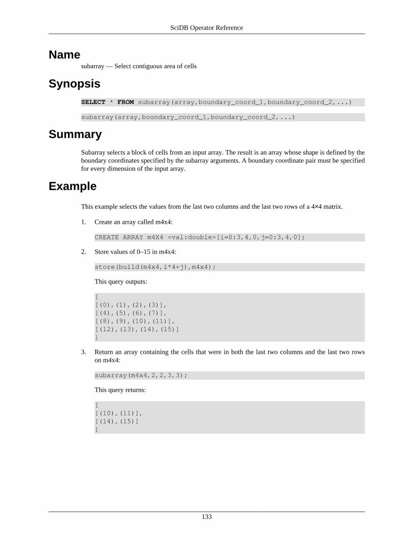
SciDB Operator Reference
133
Namesubarray — Select contiguous area of cells
SynopsisSELECT * FROM subarray(array,boundary_coord_1,boundary_coord_2,...)
subarray(array,boundary_coord_1,boundary_coord_2,...)
SummarySubarray selects a block of cells from an input array. The result is an array whose shape is defined by theboundary coordinates specified by the subarray arguments. A boundary coordinate pair must be specifiedfor every dimension of the input array.
Example
This example selects the values from the last two columns and the last two rows of a 4×4 matrix.
1. Create an array called m4x4:
CREATE ARRAY m4X4 <val:double>[i=0:3,4,0,j=0:3,4,0];
2. Store values of 0–15 in m4x4:
store(build(m4x4,i*4+j),m4x4);
This query outputs:
[[(0),(1),(2),(3)],[(4),(5),(6),(7)],[(8),(9),(10),(11)],[(12),(13),(14),(15)]]
3. Return an array containing the cells that were in both the last two columns and the last two rowson m4x4:
subarray(m4x4,2,2,3,3);
This query returns:
[[(10),(11)],[(14),(15)]]

SciDB Operator Reference
134
Namesubstitute — Substitute new value for null values in an array
SynopsisSELECT * FROM substitute(null_array,substitute_array[, attribute_1,attribute_2,...]);
substitute(null_array,substitute_array[,attribute_1,attribute_2,...]);
SummarySubstitute null values in one array with non-null values from another array. The arrays must have the samedimension start index.
The substitute operator will render attributes in null_array non-nullable. If an attribute has null values,you can use this operator to substitute null values in the array and change the nullability of the attributein the schema.
ExampleThis example replaces all null values in an array with zero.
1. Create an array m4x4_null with a nullable attribute:
CREATE ARRAY m4x4_null <val:double null>[i=0:3,4,0,j=0:3,4,0];
2. Store null in the second row of m4x4_null and 100 in all the other cells:
store(build(m4x4_null,iif(i=1,null,100)),m4x4_null);
3. Create a single-cell array called substitute_array
CREATE ARRAY substitute_array <missing:double>[i=0:0,1,0];
4. Put value 0 into substitute_array:
store(build(substitute_array,0),substitute_array);
5. Use the substitute operator to replace the null-valued cells in m4x4_null with 0-valued cells:
substitute(m4x4_null,substitute_array);
This query outputs:
[[(100),(100),(100),(100)],[(0),(0),(0),(0)],[(100),(100),(100),(100)],[(100),(100),(100),(100)]]

SciDB Operator Reference
135
Namesum — Sum attribute values
SynopsisSELECT * FROM sum(array,attribute[,dimension1,dimension2,...])
Summary
Note
The sum operator offers the same functionality as the sum aggregate. See sum aggregate referencepage for more information.
Example
This example sums the columns and rows of a 3×3 array.
1. Create a 1-attribute, 2-dimensional array called m3x3:
CREATE ARRAY m3x3 <val:double>[i=0:2,3,0,j=0:2,3,0];
2. Store values of 0–8 in m3x3:
store(build(m3x3,i*3+j),m3x3);
[[(0),(1),(2)],[(3),(4),(5)],[(6),(7),(8)]]
3. Sum the values of m3x3 along dimension j. This sums the columns of m3x3:
sum(m3x3,val,j);
This query outputs:
[(9),(12),(15)]
4. Sum the values of m3x3 along dimension i. This sums the rows of m3x3:
sum(m3x3,val,i);
This query outputs:
[(3),(12),(21)]

SciDB Operator Reference
136
Namethin — Select data from an array dimension at fixed intervals
SynopsisSELECT * FROM thin(array,start_1,step_1,start_2,step_2,...);
thin(array,start_1,step_1,start_2,step_2,...);
SummaryThe thin operator selects regularly spaced elements of the array in each dimension. The selection criteriaare specified by the starting dimension value start_1 and the number of cells to skip using step_1for each dimension of the input array. The dimension chunk size must be evenly divisible by the step size.
Example
This example selects values from a 6×6 array.
1. Create an array m6x6:
CREATE ARRAY m6x6 <val:double>[i=0:5,6,0,j=0:5,6,0];
2. Put values of 1–35 into m6x6:
store(build(m6x6,i*6+j),m6x6);
[[(0),(1),(2),(3),(4),(5)],[(6),(7),(8),(9),(10),(11)],[(12),(13),(14),(15),(16),(17)],[(18),(19),(20),(21),(22),(23)],[(24),(25),(26),(27),(28),(29)],[(30),(31),(32),(33),(34),(35)]]
3. Select every other column of m6x6, starting at the first column;
thin(m6x6,0,1,0,2);
This query outputs:
[[(0),(2),(4)],[(6),(8),(10)],[(12),(14),(16)],[(18),(20),(22)],[(24),(26),(28)],[(30),(32),(34)]]
4. Select every other row from m6x6, starting at the first row;
thin(m6x6,0,1,0,2);

SciDB Operator Reference
137
This query outputs:
[[(0),(1),(2),(3),(4),(5)],[(12),(13),(14),(15),(16),(17)],[(24),(25),(26),(27),(28),(29)]]
5. Select every other value from m6x6, starting at the second column;
thin(m6x6,1,2,1,2);
This query outputs:
[[(7),(9),(11)],[(19),(21),(23)],[(31),(33),(35)]]
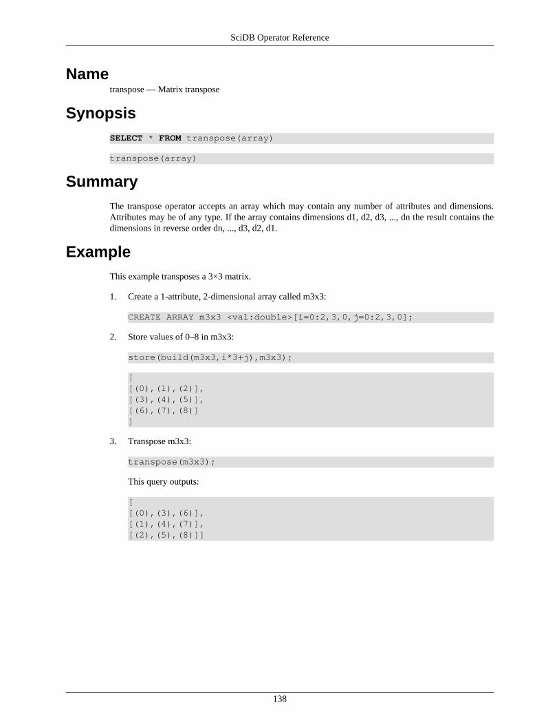
SciDB Operator Reference
138
Nametranspose — Matrix transpose
SynopsisSELECT * FROM transpose(array)
transpose(array)
SummaryThe transpose operator accepts an array which may contain any number of attributes and dimensions.Attributes may be of any type. If the array contains dimensions d1, d2, d3, ..., dn the result contains thedimensions in reverse order dn, ..., d3, d2, d1.
ExampleThis example transposes a 3×3 matrix.
1. Create a 1-attribute, 2-dimensional array called m3x3:
CREATE ARRAY m3x3 <val:double>[i=0:2,3,0,j=0:2,3,0];
2. Store values of 0–8 in m3x3:
store(build(m3x3,i*3+j),m3x3);
[[(0),(1),(2)],[(3),(4),(5)],[(6),(7),(8)]]
3. Transpose m3x3:
transpose(m3x3);
This query outputs:
[[(0),(3),(6)],[(1),(4),(7)],[(2),(5),(8)]]

SciDB Operator Reference
139
Nameunload_library — Unload a plugin
Synopsisunload_library('library_name')
SummaryUnload a plug-in from the current SciDB instance.
Note
The unload_library operator provides the same functionality as the AQL UNLOAD LIBRARY'library_name' statement.
ExampleThis example loads and unloads the example plug-in librational.so.
load_library('librational')unload_library ('librational')
The file extension is not included in the library name.

SciDB Operator Reference
140
Nameunpack — Transform multidimensional array to single dimension
SynopsisSELECT * INTO vector FROM unpack(array,attribute_name)
store(unpack(array,attribute_name),vector)
SummaryThe unpack operator unpacks a multidimensional array into a single-dimensional array creating newattributes to represent source array dimension values. The result array has a single zero-based dimensionand arguments combining attributes of the input array. The name for the new single dimension is passedto the operator as the second argument.
ExampleThis example takes 2-dimensional, 1-attribute array and outputs a 1-dimensional, 3-attribute array.
1. Create a 1-attribute, 2-dimensional array called m3x3:
CREATE ARRAY m3x3 <val:double>[i=0:2,3,0,j=0:2,3,0];
2. Store values of 0–8 in m3x3:
store(build(m3x3,i*3+j),m3x3);
[[(0),(1),(2)],[(3),(4),(5)],[(6),(7),(8)]]
3. Create a new attribute called val2 containing values 100–108 and store the resulting array asm3x3_2attr:
store(apply(m3x3,val2,val+100),m3x3_2attr);
This query outputs:
[[(0,100),(1,101),(2,102)],[(3,103),(4,104),(5,105)],[(6,106),(7,107),(8,108)]]
4. Unpack m3x3_2attr into a 1-dimensional array.
This query outputs:
[(0,0,0,100),

SciDB Operator Reference
141
(0,1,1,101),(0,2,2,102),(1,0,3,103),(1,1,4,104),(1,2,5,105),(2,0,6,106),(2,1,7,107),(2,2,8,108)]
The first two values in each cell are the dimensional indices, and the second two are the attributevalues.

SciDB Operator Reference
142
Namevar — Variance
SynopsisSELECT * FROM var(array,attribute[,dimension1,dimension2,...])
SummaryThe var operator returns the variance of a set of values taken from an array attribute.
Note
The var operator provides the same functionality as the var aggregate. See the var aggregatereference page for more information.
ExampleThis example finds the variance of each row of a 2-dimensional array.
1. Create a 1-attribute, 2-dimensional array called m3x3:
CREATE ARRAY m3x3 <val:double>[i=0:2,3,0,j=0:2,3,0];
2. Store values of random values between 0 and 1 in m3x3:
store(build(m3x3,random()%9/10.0),m3x3);
[[(0.5),(0.6),(0)],[(0.8),(0.8),(0.4)],[(0.1),(0.8),(0.6)]]
3. Select the variance of each row of m3x3:
var(m3x3,val,i);
This query returns:
[(0.103333),(0.0533333),(0.13)]

SciDB Operator Reference
143
Nameversions — Show array versions
SynopsisSELECT * FROM versions(named_array);
versions(named_array);
SummaryThe versions operator lists all versions of an array in the SciDB namespace. The output of the versionscommand is a list of versions, each of which has a version ID and a datestamp which is the date and timeof creation of that version. The argument named_array must be an array that was previously createdand stored in the SciDB namespace.
ExampleThis example creates an array, updates it twice, and then returns the first version of the array.
1. Create an array called m1:
CREATE ARRAY m1 <val:double>[i=0:9,10,0];
2. Store 1 in each cell of m1:
store(build(m1,1),m1);
3. Update every cell to have value 100:
store(build(m1,100),m1);
4. Use the versions command to see the two versions of m1 that you created:
versions(m1);
5. Use the scan operator and the '@1' array name extension to display the first version of m1.
scan(m1@1);
This query outputs:
[(1),(1),(1),(1),(1),(1),(1),(1),(1),(1)]

SciDB Operator Reference
144
Namewindow — Compute aggregates over moving window
SynopsisSELECT * FROM window(array,grid_1,grid_2,...,grid_N,aggregate_call_1[,aggrgegate_call_2, ...]
SummaryCompute one or more aggregates of any of an array's attributes over a moving window.
Note
The AFL window operator provides the same functionality as the AQL SELECT ... FROM ...WINDOW statement. See the User's Guide chapter on Aggregates for more information.
ExampleThis example calculates a running sum for a 3×3 window on a 4×4 array.
1. Create an array called m4x4:
CREATE ARRAY m4X4 <val:double>[i=0:3,4,0,j=0:3,4,0];
2. Store values of 0–15 in m4x4:
store(build(m4x4,i*4+j),m4x4);
This query outputs:
[[(0),(1),(2),(3)],[(4),(5),(6),(7)],[(8),(9),(10),(11)],[(12),(13),(14),(15)]]
3. Return the maximum and minimum values on a moving 3×3 window on m4x4:
window(m4x4,3,3,max(val),min(val));
This query returns:
[[(5,0),(6,0),(7,1),(7,2)],[(9,0),(10,0),(11,1),(11,2)],[(13,4),(14,4),(15,5),(15,6)],[(13,8),(14,8),(15,9),(15,10)]]

SciDB Operator Reference
145
Namexgrid — Expand single array element to grid
SynopsisSELECT * FROM xgrid(array,scale_1[,scale_2,..., scale_N])
xgrid(array,scale_1[,scale_2,..., scale_N])
SummaryThe xgrid operators scales an input array by repeating cells of the original array specified number of timesin a contiguous subregion. xgrid takes one scale argument for every dimension in array. The outputarray has the same number of dimensions and attributes as the input array.
Example
This example scales each cell of a 2-dimensional array into a 2×2 subarray.
1. Create an array called m3x3:
CREATE ARRAY m3x3 <val:double> [i=0:2,3,0,j=0:2,3,0];
2. Put values of 0–8 into m3x3:
store(build(m3x3,i*3+j),m3x3);
3. Expand each cell of m3x3 into a 2×2 subgrid. Store the resulting array as m6x6:
store(xgrid(m3x3,2,2),m6x6);
This query returns:
[[(0),(0),(1),(1),(2),(2)],[(0),(0),(1),(1),(2),(2)],[(3),(3),(4),(4),(5),(5)],[(3),(3),(4),(4),(5),(5)],[(6),(6),(7),(7),(8),(8)],[(6),(6),(7),(7),(8),(8)]]