1

SCHOOL OF MECHANICAL

DEPARTMENT OF MECHANICAL

UNIT – I – Heat and Mass Transfer – SMEA1504

2

UNIT – I

BASIC CONCEPTS IN HEAT TRANSFER

1.1 Heat Energy and Heat Transfer

Heat is a form of energy in transition and it flows from one system to another, without

transfer of mass, whenever there is a temperature difference between the systems. The process of

heat transfer means the exchange in internal energy between the systems and in almost every

phase of scientific and engineering work processes, we encounter the flow of heat energy.

1.2 Importance of Heat Transfer

Heat transfer processes involve the transfer and conversion of energy and therefore, it is

essential to determine the specified rate of heat transfer at a specified temperature difference.

The design of equipments like boilers, refrigerators and other heat exchangers require a detailed

analysis of transferring a given amount of heat energy within a specified time. Components like

gas/steam turbine blades, combustion chamber walls, electrical machines, electronic gadgets,

transformers, bearings, etc require continuous removal of heat energy at a rapid rate in order to

avoid their overheating. Thus, a thorough understanding of the physical mechanism of heat flow

and the governing laws of heat transfer are a must.

1.3 Modes of Heat Transfer

The heat transfer processes have been categorized into three basic modes: Conduction,

Convection and Radiation.

Conduction – It is the energy transfer from the more energetic to the less energetic particles of a

substance due to interaction between them, a microscopic activity.

Convection - It is the energy transfer due to random molecular motion a long with the

macroscopic motion of the fluid particles.

Radiation - It is the energy emitted by matter which is at finite temperature. All forms of

matter emit radiation attributed to changes m the electron configuration of the

constituent atoms or molecules The transfer of energy by conduction and

convection requires the presence of a material medium whereas radiation does

not. In fact radiation transfer is most efficient in vacuum.

3

All practical problems of importance encountered in our daily life Involve at least two,

and sometimes all the three modes occuring simultaneously When the rate of heat flow is

constant, i.e., does not vary with time, the process is called a steady state heat transfer process.

When the temperature at any point in a system changes with time, the process is called unsteady

or transient process. The internal energy of the system changes in such a process when the

temperature variation of an unsteady process describes a particular cycle (heating or cooling of a

budding wall during a 24 hour cycle), the process is called a periodic or quasi-steady heat

transfer process.

Heat transfer may take place when there is a difference In the concentration of the

mixture components (the diffusion thermoeffect). Many heat transfer processes are accompanied

by a transfer of mass on a macroscopic scale. We know that when water evaporates, the heal

transfer is accompanied by the transport of the vapour formed through an air-vapour mixture.

The transport of heat energy to steam generally occurs both through molecular interaction and

convection. The combined molecular and convective transport of mass is called convection mass

transfer and with this mass transfer, the process of heat transfer becomes more complicated.

1.4 Thermodynamics and Heat Transfer-Basic Difference

Thermodynamics is mainly concerned with the conversion of heat energy into other

useful forms of energy and IS based on (i) the concept of thermal equilibrium (Zeroth Law), (ii)

the First Law (the principle of conservation of energy) and (iii) the Second Law (the direction in

which a particular process can take place). Thermodynamics is silent about the heat energy

exchange mechanism. The transfer of heat energy between systems can only take place whenever

there is a temperature gradient and thus. Heat transfer is basically a non-equilibrium

phenomenon. The Science of heat transfer tells us the rate at which the heat energy can be

transferred when there IS a thermal non-equilibrium. That IS, the science of heat transfer seeks

to do what thermodynamics is inherently unable to do.

However, the subjects of heat transfer and thermodynamics are highly complimentary.

Many heat transfer problems can be solved by applying the principles of conservation of energy

(the First Law)

4

1.5 Dimension and Unit

Dimensions and units are essential tools of engineering. Dimension is a set of basic

entities expressing the magnitude of our observations of certain quantities. The state of a system

is identified by its observable properties, such as mass, density, temperature, etc. Further, the

motion of an object will be affected by the observable properties of that medium in which the

object is moving. Thus a number of observable properties are to be measured to identify the state

of the system.

A unit is a definite standard by which a dimension can be described. The difference

between a dimension and the unit is that a dimension is a measurable property of the system and

the unit is the standard element in terms of which a dimension can be explicitly described with

specific numerical values.

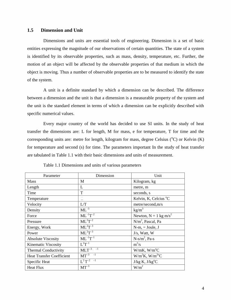
Every major country of the world has decided to use SI units. In the study of heat

transfer the dimensions are: L for length, M for mass, e for temperature, T for time and the

corresponding units are: metre for length, kilogram for mass, degree Celsius (oC) or Kelvin (K)

for temperature and second (s) for time. The parameters important In the study of heat transfer

are tabulated in Table 1.1 with their basic dimensions and units of measurement.

Table 1.1 Dimensions and units of various parameters

Parameter Dimension Unit

Mass M Kilogram, kg

Length L metre, m

Time T seconds, s

Temperature Kelvin, K, Celcius oC

Velocity L/T metre/second,m/s

Density ML–3

kg/m3

Force ML–1

T–2

Newton, N = 1 kg m/s2

Pressure ML2T

–2 N/m

2, Pascal, Pa

Energy, Work ML2T

–3 N-m, = Joule, J

Power ML2T

–3 J/s, Watt, W

Absolute Viscosity ML–1

T–1

N-s/m2, Pa-s

Kinematic Viscosity L2T

–1 m

2/s

Thermal Conductivity MLT–3 –1

W/mK, W/moC

Heat Transfer Coefficient MT–3 –1

W/m2K, W/m

2oC

Specific Heat L2 T

–2 –1 J/kg K, J/kg

oC

Heat Flux MT–3

W/m2

5

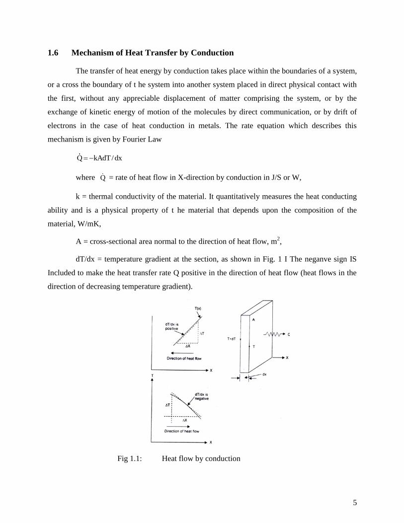
1.6 Mechanism of Heat Transfer by Conduction

The transfer of heat energy by conduction takes place within the boundaries of a system,

or a cross the boundary of t he system into another system placed in direct physical contact with

the first, without any appreciable displacement of matter comprising the system, or by the

exchange of kinetic energy of motion of the molecules by direct communication, or by drift of

electrons in the case of heat conduction in metals. The rate equation which describes this

mechanism is given by Fourier Law

Q kAdT/dx

where Q = rate of heat flow in X-direction by conduction in J/S or W,

k = thermal conductivity of the material. It quantitatively measures the heat conducting

ability and is a physical property of t he material that depends upon the composition of the

material, W/mK,

A = cross-sectional area normal to the direction of heat flow, m2,

dT/dx = temperature gradient at the section, as shown in Fig. 1 I The neganve sign IS

Included to make the heat transfer rate Q positive in the direction of heat flow (heat flows in the

direction of decreasing temperature gradient).

Fig 1.1: Heat flow by conduction

6

1.7 Thermal Conductivity of Materials

Thermal conductivity is a physical property of a substance and In general, It depends

upon the temperature, pressure and nature of the substance. Thermal conductivity of materials

are usually determined experimentally and a number of methods for this purpose are well known.

Thermal Conductivity of Gases: According to the kinetic theory of gases, the heat

transfer by conduction in gases at ordinary pressures and temperatures take place through the

transport of the kinetic energy arising from the collision of the gas molecules. Thermal

conductivity of gases depends on pressure when very low «2660 Pal or very high (> 2 × 109 Pa).

Since the specific heat of gases Increases with temperature, the thermal conductivity Increases

with temperature and with decreasing molecular weight.

Thermal Conductivity of Liquids: The molecules of a liquid are more closely spaced

and molecular force fields exert a strong influence on the energy exchange In the collision

process. The mechanism of heat propagation in liquids can be conceived as transport of energy

by way of unstable elastic oscillations. Since the density of liquids decreases with increasing

temperature, the thermal conductivity of non-metallic liquids generally decreases with increasing

temperature, except for liquids like water and alcohol because their thermal conductivity first

Increases with increasing temperature and then decreases.

Thermal Conductivity of Solids (i) Metals and Alloys: The heat transfer in metals arise

due to a drift of free electrons (electron gas). This motion of electrons brings about the

equalization in temperature at all points of t he metals. Since electrons carry both heat and

electrical energy. The thermal conductivity of metals is proportional to its electrical conductivity

and both the thermal and electrical conductivity decrease with increasing temperature. In contrast

to pure metals, the thermal conductivity of alloys increases with increasing temperature. Heat

transfer In metals is also possible through vibration of lattice structure or by elastic sound waves

but this mode of heat transfer mechanism is insignificant in comparison with the transport of

energy by electron gas. (ii) Nonmetals: Materials having a high volumetric density have a high

thermal conductivity but that will depend upon the structure of the material, its porosity and

moisture content High volumetric density means less amount of air filling the pores of the

materials. The thermal conductivity of damp materials considerably higher than the thermal

conductivity of dry material because water has a higher thermal conductivity than air. The

7

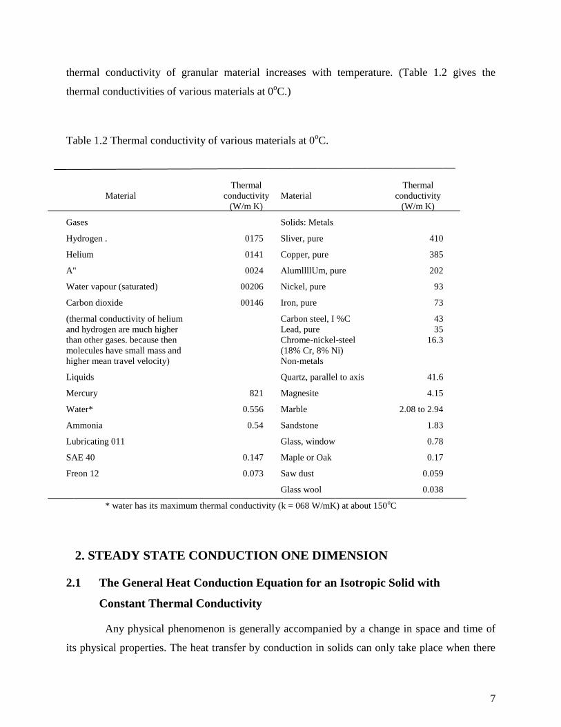
thermal conductivity of granular material increases with temperature. (Table 1.2 gives the

thermal conductivities of various materials at 0oC.)

Table 1.2 Thermal conductivity of various materials at 0oC.

Thermal Thermal

Material conductivity Material conductivity

(W/m K) (W/m K)

Gases Solids: Metals

Hydrogen . 0175 Sliver, pure 410

Helium 0141 Copper, pure 385

A" 0024 AlumllllUm, pure 202

Water vapour (saturated) 00206 Nickel, pure 93

Carbon dioxide 00146 Iron, pure 73

(thermal conductivity of helium Carbon steel, I %C 43

and hydrogen are much higher Lead, pure 35

than other gases. because then Chrome-nickel-steel 16.3

molecules have small mass and (18% Cr, 8% Ni)

higher mean travel velocity) Non-metals

Liquids Quartz, parallel to axis 41.6

Mercury 821 Magnesite 4.15

Water* 0.556 Marble 2.08 to 2.94

Ammonia 0.54 Sandstone 1.83

Lubricating 011 Glass, window 0.78

SAE 40 0.147 Maple or Oak 0.17

Freon 12 0.073 Saw dust 0.059

Glass wool 0.038

* water has its maximum thermal conductivity (k = 068 W/mK) at about 150oC

2. STEADY STATE CONDUCTION ONE DIMENSION

2.1 The General Heat Conduction Equation for an Isotropic Solid with

Constant Thermal Conductivity

Any physical phenomenon is generally accompanied by a change in space and time of

its physical properties. The heat transfer by conduction in solids can only take place when there

8

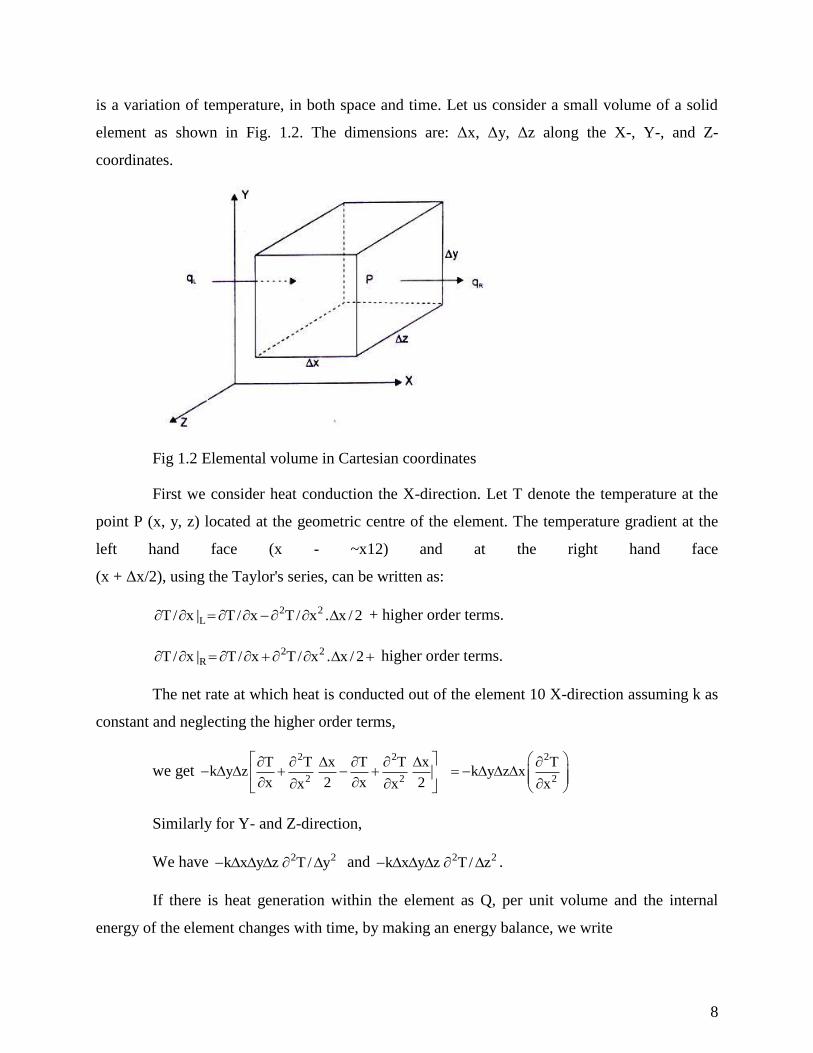
is a variation of temperature, in both space and time. Let us consider a small volume of a solid

element as shown in Fig. 1.2. The dimensions are: Δx, Δy, Δz along the X-, Y-, and Z-

coordinates.

Fig 1.2 Elemental volume in Cartesian coordinates

First we consider heat conduction the X-direction. Let T denote the temperature at the

point P (x, y, z) located at the geometric centre of the element. The temperature gradient at the

left hand face (x - ~x12) and at the right hand face

(x + Δx/2), using the Taylor's series, can be written as:

2 2LT/ x | T / x T/ x . x / 2 + higher order terms.

2 2RT/ x | T / x T/ x . x / 2 higher order terms.

The net rate at which heat is conducted out of the element 10 X-direction assuming k as

constant and neglecting the higher order terms,

we get 2 2

2 2

T T x T T xk y z

x 2 x 2x x

2

2

Tk y z x

x

Similarly for Y- and Z-direction,

We have 2 2k x y z T/ y and 2 2k x y z T/ z .

If there is heat generation within the element as Q, per unit volume and the internal

energy of the element changes with time, by making an energy balance, we write

9

Heat generated within Heat conducted away Rate of change of internal

the element from the element energy within with the element

or, 2 2 2 2 2 2vQ x y z k x y z T / x T / y T / z

c x y z T/ t

Upon simplification, 2 2 2 2 2 2v

cT / x T / y T / z Q / k T / t

k

or, 2vT Q / k 1/ T / t

where k / . c , is called the thermal diffusivity and is seen to be a physical property

of the material of which the solid is composed.

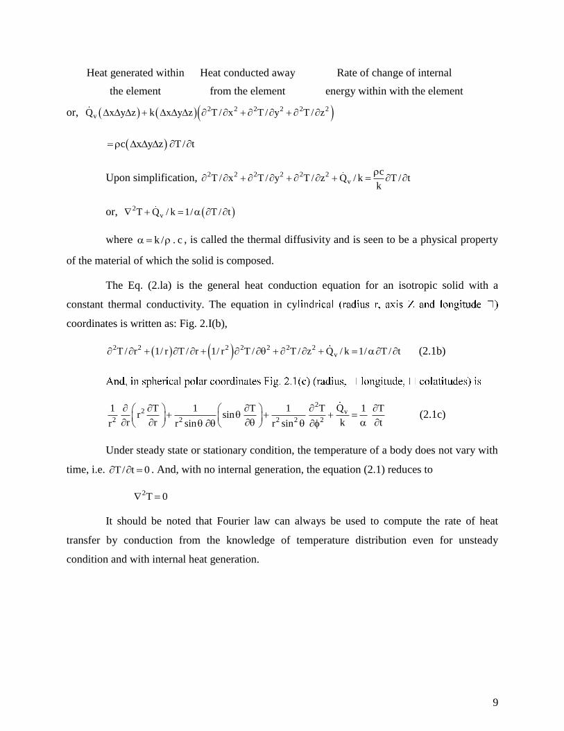
The Eq. (2.la) is the general heat conduction equation for an isotropic solid with a

constant thermal conductivity. The equation in cy

coordinates is written as: Fig. 2.I(b),

2 2 2 2 2 2 2vT / r 1/ r T / r 1/ r T / T / z Q / k 1/ T / t (2.1b)

22 v

2 2 2 2 2

Q1 T 1 T 1 T 1 Tr sin

r r k tr r sin r sin

(2.1c)

Under steady state or stationary condition, the temperature of a body does not vary with

time, i.e. T/ t 0 . And, with no internal generation, the equation (2.1) reduces to

2T 0

It should be noted that Fourier law can always be used to compute the rate of heat

transfer by conduction from the knowledge of temperature distribution even for unsteady

condition and with internal heat generation.

10

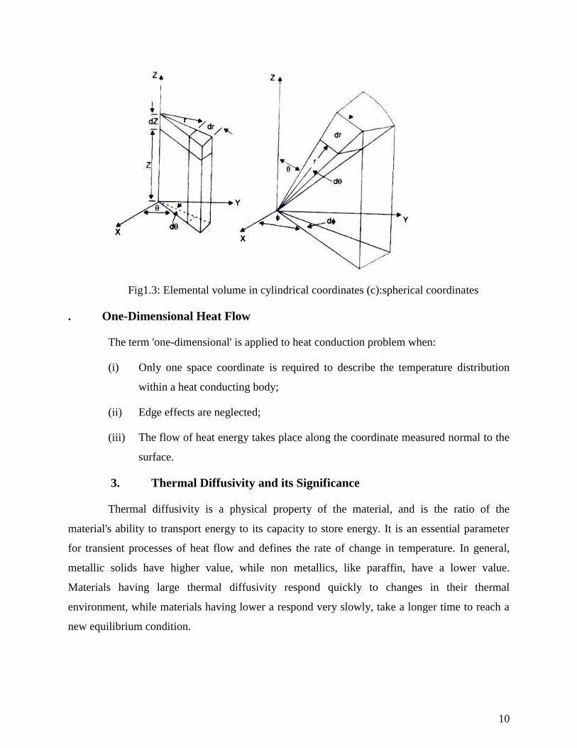
Fig1.3: Elemental volume in cylindrical coordinates (c):spherical coordinates

. One-Dimensional Heat Flow

The term 'one-dimensional' is applied to heat conduction problem when:

(i) Only one space coordinate is required to describe the temperature distribution

within a heat conducting body;

(ii) Edge effects are neglected;

(iii) The flow of heat energy takes place along the coordinate measured normal to the

surface.

3. Thermal Diffusivity and its Significance

Thermal diffusivity is a physical property of the material, and is the ratio of the

material's ability to transport energy to its capacity to store energy. It is an essential parameter

for transient processes of heat flow and defines the rate of change in temperature. In general,

metallic solids have higher value, while non metallics, like paraffin, have a lower value.

Materials having large thermal diffusivity respond quickly to changes in their thermal

environment, while materials having lower a respond very slowly, take a longer time to reach a

new equilibrium condition.

11

4. TEMPERATURE DISTRIBUTION IN I-D SYSTEMS

4.1 A Plane Wall

A plane wall is considered to be made out of a constant thermal conductivity material

and extends to infinity in the Y- and Z-direction. The wall is assumed to be homogeneous and

isotropic, heat flow is one-dimensional, under steady state conditions and losing negligible

energy through the edges of the wall under the above mentioned assumptions the Eq. (2.2)

reduces to

d2T / dx

2 = 0; the boundary conditions are: at x = 0, T = T1

Integrating the above equation, x = L, T = T2

T = C1x + C2, where C1 and C2 are two constants.

Substituting the boundary conditions, we get C2 = T1 and C1 = (T2 – T1)/L The

temperature distribution in the plane wall is given by

T = T1 – (T1 – T2) x/L (2.3)

which is linear and is independent of the material.

Further, the heat flow rate, Q /A = –k dT/dx = (T1– T2)k/L, and therefore the

temperature distribution can also be written as

1T T Q / A x / k (2.4)

i.e., “the temperature drop within the wall will increase with greater heat flow rate or

when k is small for the same heat flow rate,"

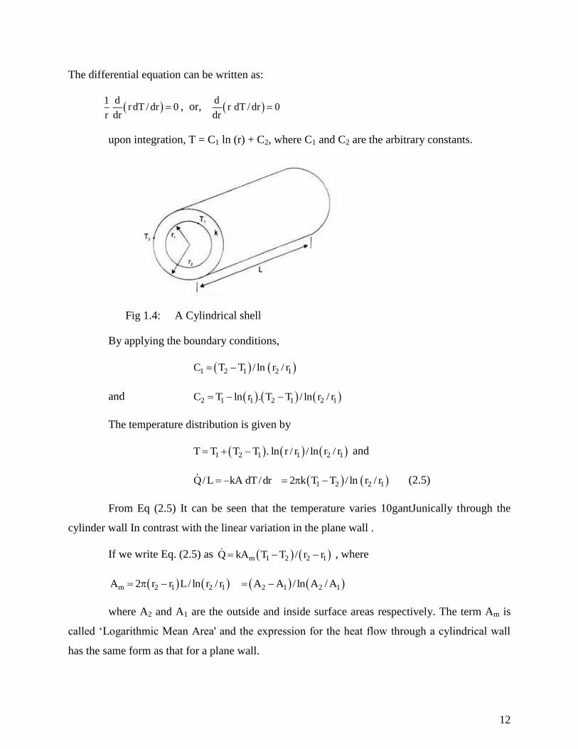
4.2 A Cylindrical Shell-Expression for Temperature Distribution

In the cylindrical system, when the temperature is a function of radial distance only and

is independent of azimuth angle or axial distance, the differential equation (2.2) would be, (Fig.

1.4)

d2T /dr

2 +(1/r) dT/dr = 0

with boundary conditions: at r = rl, T = T1 and at r = r2, T = T2.

12

The differential equation can be written as:

1 d

r dT / dr 0r dr

, or, d

r dT / dr 0dr

upon integration, T = C1 ln (r) + C2, where C1 and C2 are the arbitrary constants.

Fig 1.4: A Cylindrical shell

By applying the boundary conditions,

1 2 1 2 1C T T / ln r / r

and 2 1 1 2 1 2 1C T ln r . T T / ln r / r

The temperature distribution is given by

1 2 1 1 2 1T T T T . ln r / r / ln r / r and

Q/ L kA dT/dr 1 2 2 12 k T T / ln r / r (2.5)

From Eq (2.5) It can be seen that the temperature varies 10gantJunically through the

cylinder wall In contrast with the linear variation in the plane wall .

If we write Eq. (2.5) as m 1 2 2 1Q kA T T / r r , where

m 2 1 2 1A 2 r r L/ ln r / r 2 1 2 1A A / ln A / A

where A2 and A1 are the outside and inside surface areas respectively. The term Am is

called ‘Logarithmic Mean Area' and the expression for the heat flow through a cylindrical wall

has the same form as that for a plane wall.

13

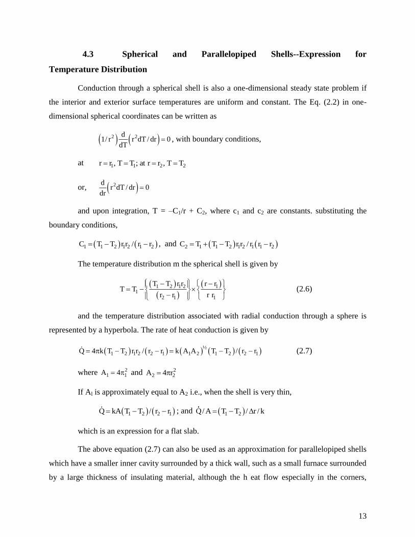
4.3 Spherical and Parallelopiped Shells--Expression for

Temperature Distribution

Conduction through a spherical shell is also a one-dimensional steady state problem if

the interior and exterior surface temperatures are uniform and constant. The Eq. (2.2) in one-

dimensional spherical coordinates can be written as

2 2d1/ r r dT / dr 0

dT , with boundary conditions,

at 1 1 2 2r r , T T ; at r r , T T

or, 2dr dT / dr 0

dr

and upon integration, T = –C1/r + C2, where c1 and c2 are constants. substituting the

boundary conditions,

1 1 2 1 2 1 2C T T r r / r r , and 2 1 1 2 1 2 1 1 2C T T T r r / r r r

The temperature distribution m the spherical shell is given by

1 2 1 2 11

2 1 1

T T r r r rT T

r r r r

(2.6)

and the temperature distribution associated with radial conduction through a sphere is

represented by a hyperbola. The rate of heat conduction is given by

½

1 2 1 2 2 1 1 2 1 2 2 1Q 4 k T T r r / r r k A A T T / r r (2.7)

where 21 1A 4 and 2

2 2A 4 r

If Al is approximately equal to A2 i.e., when the shell is very thin,

1 2 2 1Q kA T T / r r ; and 1 2Q/ A T T / r / k

which is an expression for a flat slab.

The above equation (2.7) can also be used as an approximation for parallelopiped shells

which have a smaller inner cavity surrounded by a thick wall, such as a small furnace surrounded

by a large thickness of insulating material, although the h eat flow especially in the corners,

14

cannot be strictly considered one-dimensional. It has been suggested that for (A2/A1) > 2, the rate

of heat flow can be approximated by the above equation by multiplying the geometric mean area

Am = (A1 A2)½ by a correction factor 0.725.]

4.4 Composite Surfaces

There are many practical situations where different materials are placed m layers to

form composite surfaces, such as the wall of a building, cylindrical pipes or spherical shells

having different layers of insulation. Composite surfaces may involve any number of series and

parallel thermal circuits.

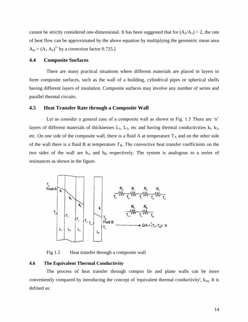
4.5 Heat Transfer Rate through a Composite Wall

Let us consider a general case of a composite wall as shown m Fig. 1.5 There are ‘n’

layers of different materials of thicknesses L1, L2, etc and having thermal conductivities kl, k2,

etc. On one side of the composite wall, there is a fluid A at temperature TA and on the other side

of the wall there is a fluid B at temperature TB. The convective heat transfer coefficients on the

two sides of the wall are hA and hB respectively. The system is analogous to a series of

resistances as shown in the figure.

Fig 1.5 Heat transfer through a composite wall

4.6 The Equivalent Thermal Conductivity

The process of heat transfer through compos lie and plane walls can be more

conveniently compared by introducing the concept of 'equivalent thermal conductivity', keq. It is

defined as:

15

n n

eq i i i

i 1 i 1

k L L / k

(2.8)

Total thickeness of the composite wall=

Total thermal resistance of the composite wall

And, its value depends on the thermal and physical properties and the thickness of each

constituent of the composite structure.

Example 1.2 A furnace wall consists of 150 mm thick refractory brick (k = 1.6 W/mK) and

150 mm thick insulating fire brick (k = 0.3 W/mK) separated by an au gap

(resistance 0 16 K/W). The outside walls covered with a 10 mm thick plaster (k =

0.14 W/mK). The temperature of hot gases is 1250°C and the room temperature

is 25°C. The convective heat transfer coefficient for gas side and air side is 45

W/m2K and 20 W/m2K. Calculate (i) the rate of heat flow per unit area of the

wall surface (ii) the temperature at the outside and Inside surface of the wall and

(iii) the rate of heat flow when the air gap is not there.

Solution: Using the nomenclature of Fig. 2.3, we have per m2 of the area, hA = 45, and

RA = 1/hA = 1/45 = 0.0222; hB = 20, and RB = 1120 = 0.05

Resistance of the refractory brick, R1 = L1/k1 = 0.15/1.6 = 0.0937

Resistance of the insulating brick, R3 = L3/k3 = 0.15/0.30 = 0.50

The resistance of the air gap, R2 = 0.16

Resistance of the plaster, R4 = 0.01/0.14 = 0.0714

Total resistance = 0.8973, m2K/W

Heat flow rate = ΔT/R = (1250-25)/0.8973= 13662 W/m2

Temperature at the inner surface of the wall

= TA – 1366.2 × 0.0222 = 1222.25

Temperature at the outer surface of the wall

= TB + 1366.2 × 0.05 = 93.31 °C

When the air gap is not there, the total resistance would be

16

0.8973 - 0.16 = 0.7373

and the heat flow rate = (1250 – 25)/0/7373 = 1661.46 W/m2

The temperature at the inner surface of the wall

= 1250 – 1660.46 × 0.0222 = 1213.12°C

i.e., when the au gap is not there, the heat flow rate increases but the temperature at the

inner surface of the wall decreases.

The overall heat transfer coefficient U with and without the air gap is

U= Q/A / T

= 13662 / (1250 – 25) = 1.115 Wm2 °C

and 1661.46/l225 = 1356 W/m2o

C

The equivalent thermal conductivity of the system without the air gap

keq = (0.15 + 0.15 + 0.01)/(0.0937 + 0.50 + 0.0714) = 0.466 W/mK.

Example 1.2 A brick wall (10 cm thick, k = 0.7 W/m°C) has plaster on one side of the wall

(thickness 4 cm, k = 0.48 W/m°C). What thickness of an insulating material (k =

0.065 W moC) should be added on the other side of the wall such that the heat loss

through the wall IS reduced by 80 percent.

Solution: When the insulating material is not there, the resistances are:

R1 = L1/k1 = 0.1/0.7 = 0.143

and R2 = 0.04/0.48 = 0.0833

Total resistance = 0.2263

Let the thickness of the insulating material is L3. The resistance would then be

L3/0.065 = 15.385 L3

Since the heat loss is reduced by 80% after the insulation is added.

Q with insulation R without insulation0.2

Q without insulation R with insulation

17

or, the resistance with insulation = 0.2263/0.2 = 01.1315

and, 15385 L3 = I 1315 – 0.2263 = 0.9052

L3 = 0.0588 m = 58.8 mm

Example 1.3 An ice chest IS constructed of styrofoam (k = 0.033 W/mK) having inside

dimensions 25 by 40 by 100 cm. The wall thickness is 4 cm. The outside surface

of the chest is exposed to air at 25°C with h = 10 W/m2K. If the chest is

completely filled with ice, calculate the time for ice to melt completely. The heat

of fusion for water is 330 kJ/kg.

Solution: If the heat loss through the comers and edges are Ignored, we have three walls of walls

through which conduction heat transfer Will occur.

(a) 2 walls each having dimensions 25 cm × 40 cm × 4 cm

(b) 2 walls each having dimensions 25 cm × 100 cm × 4 cm

(c) 2 walls each having dimensions 40 cm × 100 cm × 4 cm

The surface area for convection heat transfer (based on outside dimensions)

2(33 × 48 + 33 × 108 + 48 × 108) × 10–4

= 2.0664 m2.

Resistance due to conduction and convection can be written as

0.04 0.04 0.04 12

0.033 0.25 0.4 0.033 0.25 1 0.033 0.4 1 10 2.0664

= 40 + 0.0484 = 40.0484 K/W

Q T / R = (25 – 0.0) / 40.0484 = 0.624 W

Inside volume of the container - 0.25 × 04 × 1 = 0.1 m3

Mass of Ice stored = 800 × 0.1 = 80 kg; taking the density of Ice as 800 kg/m3. The time

required to melt 80 kg of ice is

80 330 1000t 490 days

0.624 3600 24

Example1.4 A composite furnace wall is to be constructed with two layers of materials (k1 =

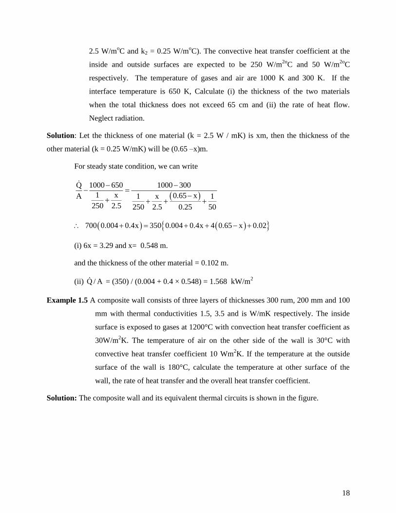
18

2.5 W/moC and k2 = 0.25 W/m

oC). The convective heat transfer coefficient at the

inside and outside surfaces are expected to be 250 W/m2o

C and 50 W/m2o

C

respectively. The temperature of gases and air are 1000 K and 300 K. If the

interface temperature is 650 K, Calculate (i) the thickness of the two materials

when the total thickness does not exceed 65 cm and (ii) the rate of heat flow.

Neglect radiation.

Solution: Let the thickness of one material (k = 2.5 W / mK) is xm, then the thickness of the

other material (k = 0.25 W/mK) will be (0.65 –x)m.

For steady state condition, we can write

Q 1000 650 1000 300

1 x 0.65 xA 1 x 1

250 2.5 250 2.5 0.25 50

700 0.004 0.4x 350 0.004 0.4x 4 0.65 x 0.02

(i) 6x = 3.29 and x= 0.548 m.

and the thickness of the other material = 0.102 m.

(ii) Q / A = (350) / (0.004 + 0.4 × 0.548) = 1.568 kW/m2

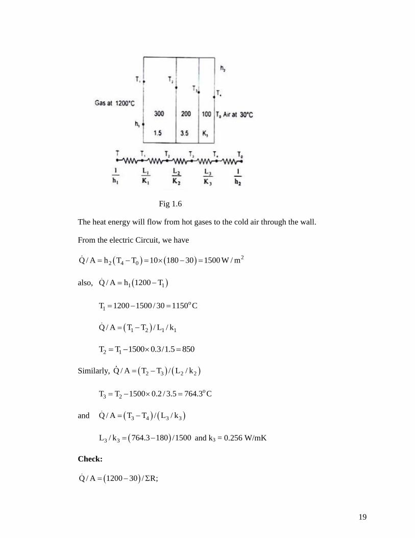
Example 1.5 A composite wall consists of three layers of thicknesses 300 rum, 200 mm and 100

mm with thermal conductivities 1.5, 3.5 and is W/mK respectively. The inside

surface is exposed to gases at 1200°C with convection heat transfer coefficient as

30W/m2K. The temperature of air on the other side of the wall is 30°C with

convective heat transfer coefficient 10 Wm2K. If the temperature at the outside

surface of the wall is 180°C, calculate the temperature at other surface of the

wall, the rate of heat transfer and the overall heat transfer coefficient.

Solution: The composite wall and its equivalent thermal circuits is shown in the figure.

19

Fig 1.6

The heat energy will flow from hot gases to the cold air through the wall.

From the electric Circuit, we have

22 4 0Q / A h T T 10 180 30 1500 W / m

also, 1 1Q / A h 1200 T

o

1T 1200 1500 / 30 1150 C

1 2 1 1Q / A T T / L / k

2 1T T 1500 0.3/1.5 850

Similarly, 2 3 2 2Q / A T T / L / k

o

3 2T T 1500 0.2 / 3.5 764.3 C

and 3 4 3 3Q / A T T / L / k

3 3L / k 764.3 180 /1500 and k3 = 0.256 W/mK

Check:

Q / A 1200 30 / R;

20

where 1 1 1 2 2 3 3 2R 1/ h L / k L / k L / k 1/ h

R 1/30 0.3/1.5 0.2/3.5 0.1/ 0.256 1/10 0.75

and 2Q / A 1170 / 0.78 1500 W / m

The overall heat transfer coefficient, 2U 1/ R 1/ 0.78 1.282 W / m K

Since the gas temperature is very high, we should consider the effects of radiation also.

Assuming the heat transfer coefficient due to radiation = 3.0 W/m2K the electric circuit would

be:

The combined resistance due to convection and radiation would be

2oc r

1 2

c r

1 1 1 1 1h h 60W / m C

1 1R R R

h h

1 1Q / A 1500 60 T T 60 1200 T

o1

1500T 1200 1175 C

60

again, o1 2 1 1 2 1Q / A T T / L / k T T 1500 0.3/1.5 875 C

and o

3 2T T 1500 0.2 / 3.5 789.3 C

3 3 3L / k 789.3 180 /1500; k 0.246 W / mK

1 0.3 0.2 0.2 0.1 1

R 0.7860 1.5 1.5 3.5 0.246 10

and 2U 1/ R 1.282 W / m K

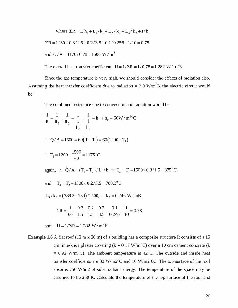
Example 1.6 A flat roof (12 m x 20 m) of a building has a composite structure It consists of a 15

cm lime-khoa plaster covering (k = 0 17 W/m°C) over a 10 cm cement concrete (k

= 0.92 W/m°C). The ambient temperature is 42°C. The outside and inside heat

transfer coefficients are 30 W/m2°C and 10 W/m2 0C. The top surface of the roof

absorbs 750 W/m2 of solar radiant energy. The temperature of the space may be

assumed to be 260 K. Calculate the temperature of the top surface of the roof and

21

the amount of water to be sprinkled uniformly over the roof surface such that the

inside temperature is maintained at 18°C.

Solution: The physical system is shown in Fig. 1.7 and it is assumed we have one-dimensional

flow, properties are constant and steady state conditions prevail.

Fig 1.7

Let the temperature of the top surface be T1°C.

Heat lost by thee top surface by convection to the surroundings is

c 1 1Q / A h T 30 T 42 30T 1260

Heat energy conducted inside through the roof = T / R

or, 11

1 2

1 2 2

T 18Q 0.15 0.1 1T 18 /

L L 1A 0.17 0.92 10

k k h

= 0.918 (T1 – 18)

Assuming that the top surface of the roof behaves like a black body, energy lost by

radiation.

4 4

r 1Q / A T 273 260

48

15.67 10 T 273 259.1

By making an energy balance on the top surface of the roof,

Energy coming in = Energy going out

750 = (30T, -1260)+ 0.918 (T1-18) + 5.67 × 10–8

(T1 + 273)4 - 259.1

or, 2285.624 = 30.918 T1 + 5.67 × 10–8

(T1 + 273)4

Solving by trial and error, T1 = 53.4°C, and the total energy conducted through the roof

22

per hour is

0.918 (53.4 – 18) × (12 × 20) × 3600 = 28077.58 kJ/hr

Assuming the latent heat of vaporization of water as 2430 kJ/kg, the quantity of water to

be sprinkled over the surface such that it evaporates and consumes 28077.58 kJ/hr, is

wM = 28077.58/2430 = 11.55 kg/hr.

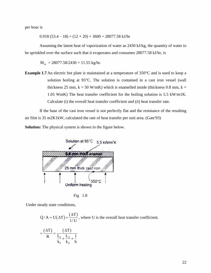
Example 1.7 An electric hot plate is maintained at a temperature of 350°C and is used to keep a

solution boiling at 95°C. The solution is contained in a cast iron vessel (wall

thickness 25 mm, k = 50 W/mK) which is enamelled inside (thickness 0.8 mm, k =

1.05 WmK) The heat transfer coefficient for the boiling solution is 5.5 kW/m1K.

Calculate (i) the overall heat transfer coefficient and (ii) heat transfer rate.

If the base of the cast iron vessel is not perfectly flat and the resistance of the resulting

air film is 35 m2K1kW, calculated the rate of heat transfer per unit area. (Gate'93)

Solution: The physical system is shown in the figure below.

Fig 1.8

Under steady state conditions,

T

Q / A U T1/ U

, where U is the overall heat transfer coefficient.

1 2

1 2

T T

L L 1R

k k h

23

Therefore,

1 2

1 2

L L 11/ U

k k h

0.025 0.0008 10.00144

50 1.05 5500

U = 692.65 W/m2K

Q / A U T = 692.65 × (350 – 95) = 176.65 kW/m2.

With the presence of air film at the base, the total resistance to heat flow would be:

0.00144 + 0.035 = 0.03644 m2K/W

and the rate of heat transfer, Q / A = 255/0.03644 = 7 kW/m2.

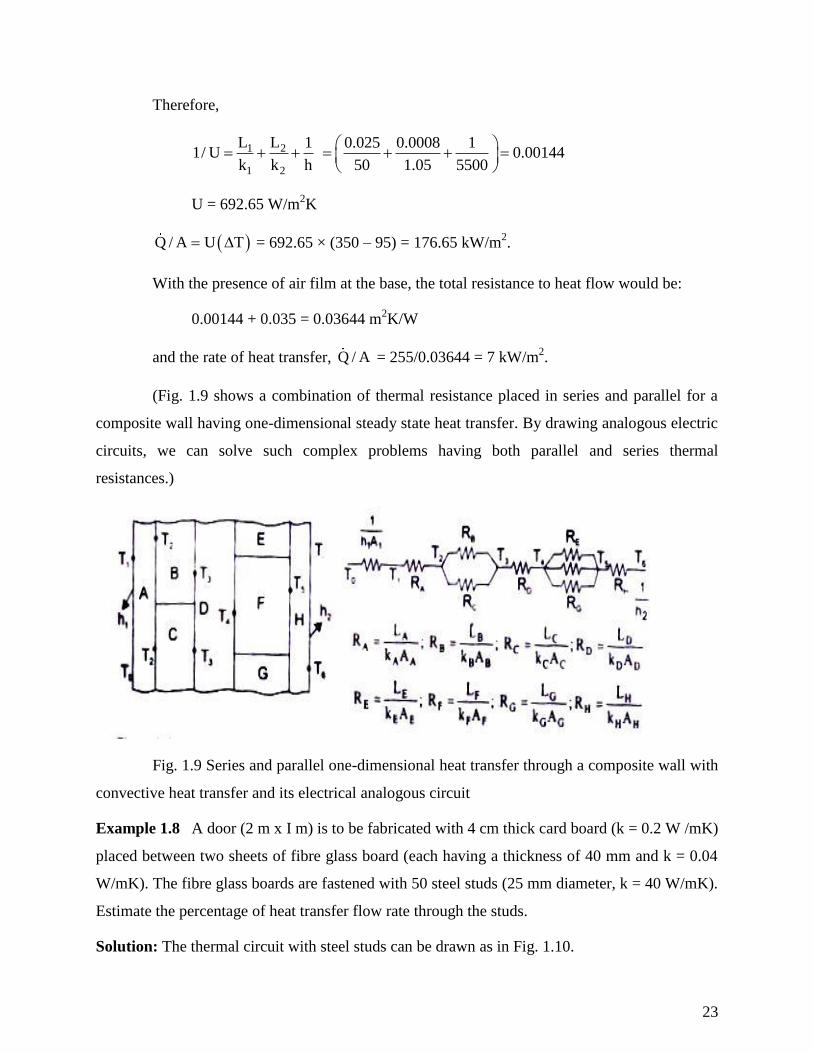
(Fig. 1.9 shows a combination of thermal resistance placed in series and parallel for a

composite wall having one-dimensional steady state heat transfer. By drawing analogous electric

circuits, we can solve such complex problems having both parallel and series thermal

resistances.)

Fig. 1.9 Series and parallel one-dimensional heat transfer through a composite wall with

convective heat transfer and its electrical analogous circuit

Example 1.8 A door (2 m x I m) is to be fabricated with 4 cm thick card board (k = 0.2 W /mK)

placed between two sheets of fibre glass board (each having a thickness of 40 mm and k = 0.04

W/mK). The fibre glass boards are fastened with 50 steel studs (25 mm diameter, k = 40 W/mK).

Estimate the percentage of heat transfer flow rate through the studs.

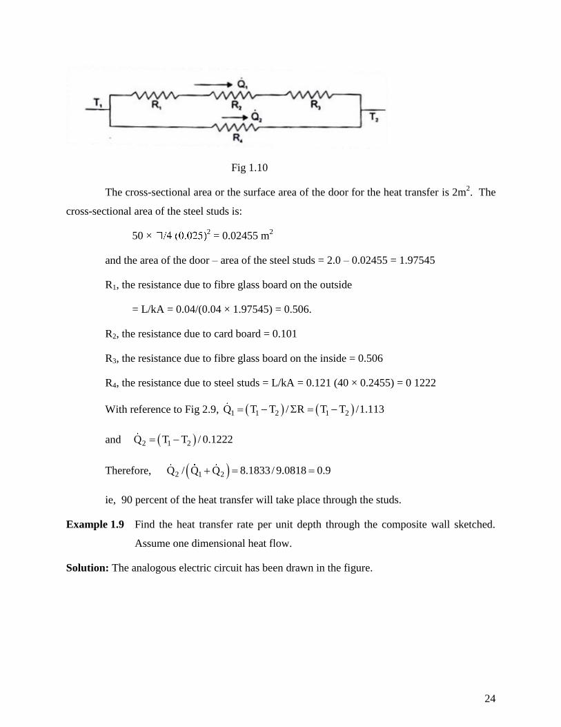
Solution: The thermal circuit with steel studs can be drawn as in Fig. 1.10.

24

Fig 1.10

The cross-sectional area or the surface area of the door for the heat transfer is 2m2. The

cross-sectional area of the steel studs is:

50 × 2 = 0.02455 m

2

and the area of the door – area of the steel studs = 2.0 – 0.02455 = 1.97545

R1, the resistance due to fibre glass board on the outside

= L/kA = 0.04/(0.04 × 1.97545) = 0.506.

R2, the resistance due to card board = 0.101

R3, the resistance due to fibre glass board on the inside = 0.506

R4, the resistance due to steel studs = L/kA = 0.121 (40 × 0.2455) = 0 1222

With reference to Fig 2.9, 1 1 2 1 2Q T T / R T T /1.113

and 2 1 2Q T T / 0.1222

Therefore, 2 1 2Q / Q Q 8.1833/ 9.0818 0.9

ie, 90 percent of the heat transfer will take place through the studs.

Example 1.9 Find the heat transfer rate per unit depth through the composite wall sketched.

Assume one dimensional heat flow.

Solution: The analogous electric circuit has been drawn in the figure.

25

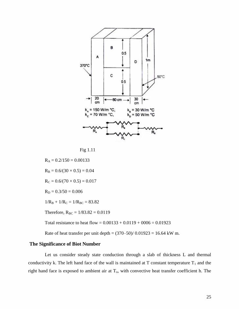
Fig 1.11

RA = 0.2/150 = 0.00133

RB = 0.6/(30 × 0.5) = 0.04

RC = 0.6/(70 × 0.5) = 0.017

RD = 0.3/50 = 0.006

1/RB + 1/RC = 1/RBC = 83.82

Therefore, RBC = 1/83.82 = 0.0119

Total resistance to heat flow = 0.00133 + 0.0119 + 0006 = 0.01923

Rate of heat transfer per unit depth = (370–50)/ 0.01923 = 16.64 kW m.

The Significance of Biot Number

Let us consider steady state conduction through a slab of thickness L and thermal

conductivity k. The left hand face of the wall is maintained at T constant temperature T1 and the

right hand face is exposed to ambient air at To, with convective heat transfer coefficient h. The

26

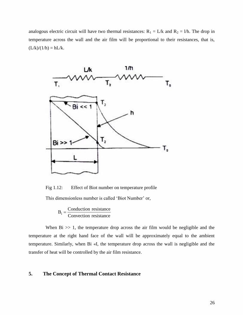
analogous electric circuit will have two thermal resistances: R1 = L/k and R2 = l/h. The drop in

temperature across the wall and the air film will be proportional to their resistances, that is,

(L/k)/(1/h) = hL/k.

Fig 1.12: Effect of Biot number on temperature profile

This dimensionless number is called ‘Biot Number’ or,

i

Conduction resistanceB

Convection resistance

When Bi >> 1, the temperature drop across the air film would be negligible and the

temperature at the right hand face of the wall will be approximately equal to the ambient

temperature. Similarly, when Bi «I, the temperature drop across the wall is negligible and the

transfer of heat will be controlled by the air film resistance.

5. The Concept of Thermal Contact Resistance

27

Heat flow rate through composite walls are usually analysed on the assumptions that -

(i) there is a perfect contact between adjacent layers, and (ii) the temperature at the interface of

the two plane surfaces is the same. However, in real situations, this is not true. No surface, even

a so-called 'mirror-finish surface', is perfectly smooth ill a microscopic sense. As such, when two

surfaces are placed together, there is not a single plane of contact. The surfaces touch only at

limited number of spots, the aggregate of which is only a small fraction of the area of the surface

or 'contact area'. The remainder of the space between the surfaces may be filled with air or other

fluid. In effect, this introduces a resistance to heat flow at the interface. This resistance IS called

'thermal contact resistance' and causes a temperature drop between the materials at the interfaces

as shown In Fig. 2.12. (That is why, Eskimos make their houses having double ice walls

separated by a thin layer of air, and in winter, two thin woolen blankets are more comfortable

than one woolen blanket having double thickness.)

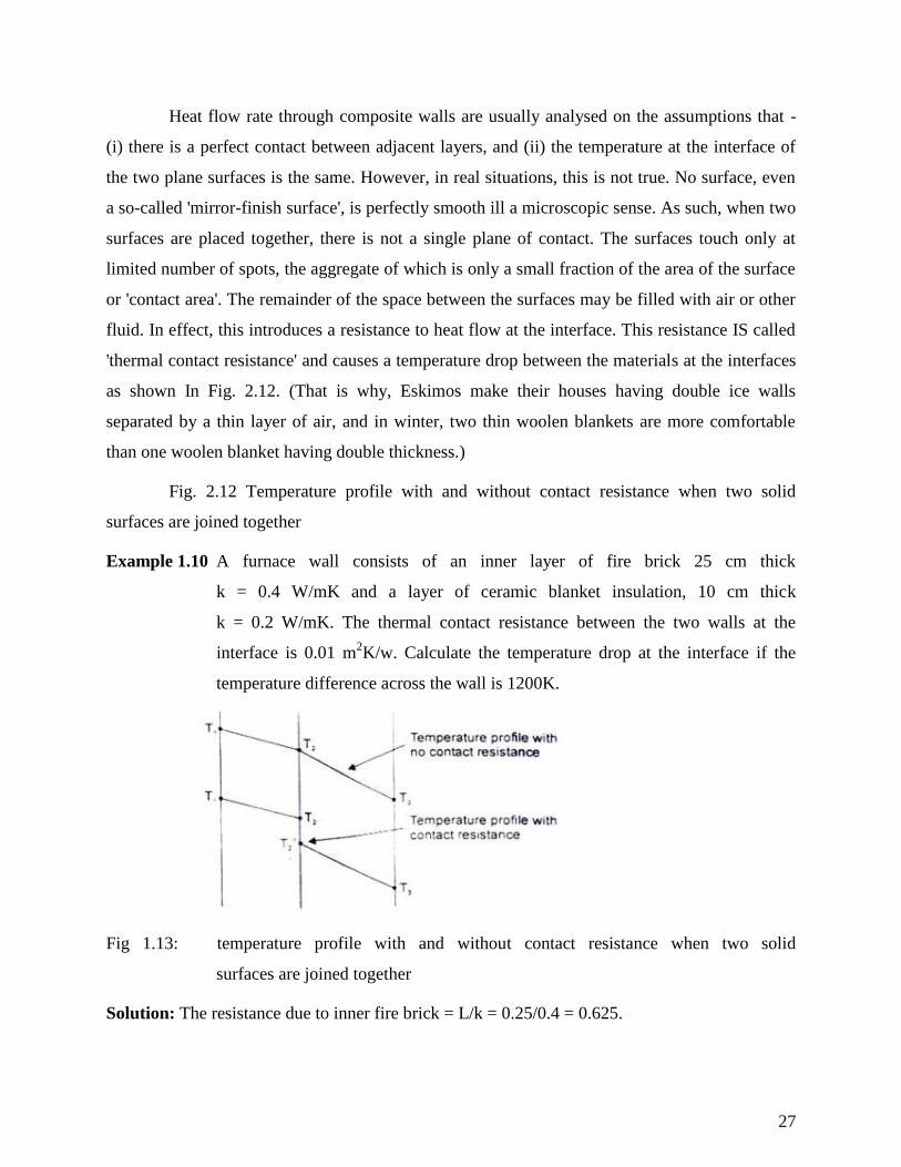
Fig. 2.12 Temperature profile with and without contact resistance when two solid

surfaces are joined together

Example 1.10 A furnace wall consists of an inner layer of fire brick 25 cm thick

k = 0.4 W/mK and a layer of ceramic blanket insulation, 10 cm thick

k = 0.2 W/mK. The thermal contact resistance between the two walls at the

interface is 0.01 m2K/w. Calculate the temperature drop at the interface if the

temperature difference across the wall is 1200K.

Fig 1.13: temperature profile with and without contact resistance when two solid

surfaces are joined together

Solution: The resistance due to inner fire brick = L/k = 0.25/0.4 = 0.625.

28

The resistance of the ceramic insulation = 0.1/0.2 = 0.5

Total thermal resistance = 0.625 + 0.01 + 0.5 = 1 135

Rate of heat flow, Q / A = 2

Temperature drop at the interface,

T Q / A × R = 1057.27 × 0.01 = 10.57 K

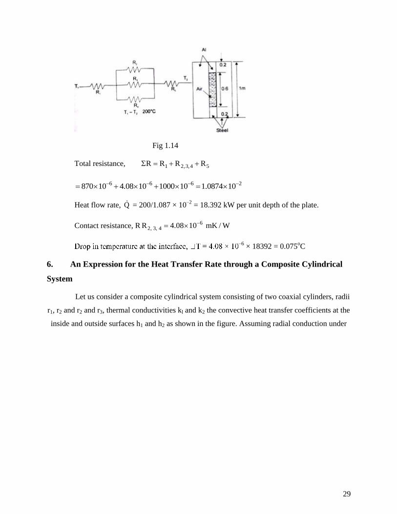
Example 1.11 A 20 cm thick slab of aluminium (k = 230 W/mK) is placed in contact with a 15

cm thick stainless steel plate (k = 15 W/mK). Due to roughness, 40 percent of the

area is in direct contact and the gap (0.0002 m) is filled with air (k = 0.032 W/mK).

The difference in temperature between the two outside surfaces of the plate is

200°C Estimate (i) the heat flow rate, (ii) the contact resistance, and (iii) the drop in

temperature at the interface.

Solution: Let us assume that out of 40% area m direct contact, half the surface area is occupied

by steel and half is occupied by aluminium.

The physical system and its analogous electric circuits is shown in Fig. 2.13.

1

0.2R 0.00087

230 1

, 6

2

0.0002R 4.348 10

230 0.2

23

0.0002R 1.04 10

0.032 0.6

, 54

0.0002R 6.667 10

15 0.2

and 5

0.15R 0.01

15 1

Again 2,3, 4 2 3 41/ R 1/ R 1/ R 1/ R

5 4 42.3 10 96.15 1.5 10 24.5 10

Therefore, 62, 3, 4R 4.08 10

29

Fig 1.14

Total resistance, 1 2,3,4 5R R R R

6 6 6 2870 10 4.08 10 1000 10 1.0874 10

Heat flow rate, Q = 200/1.087 × 10–2

= 18.392 kW per unit depth of the plate.

Contact resistance, R 62, 3, 4R 4.08 10 mK / W

–6 × 18392 = 0.075

oC

6. An Expression for the Heat Transfer Rate through a Composite Cylindrical

System

Let us consider a composite cylindrical system consisting of two coaxial cylinders, radii

r1, r2 and r2 and r3, thermal conductivities kl and k2 the convective heat transfer coefficients at the

inside and outside surfaces h1 and h2 as shown in the figure. Assuming radial conduction under

30

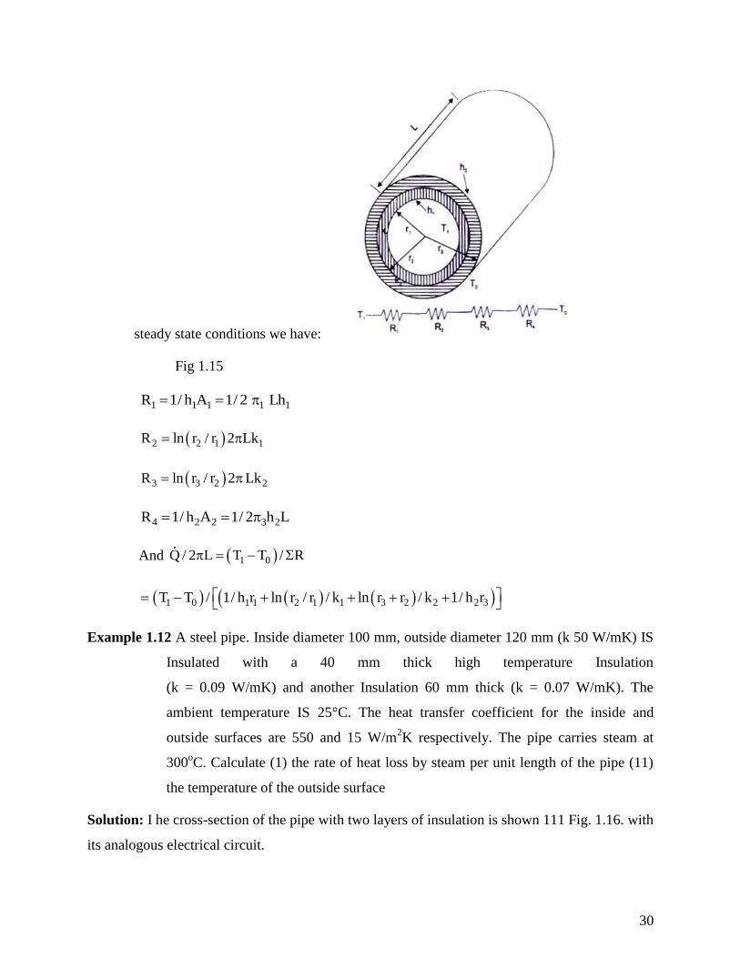
steady state conditions we have:

Fig 1.15

1 1 1 1 1R 1/ h A 1/ 2 Lh

2 2 1 1R ln r / r 2 Lk

3 3 2 2R ln r / r 2 Lk

4 2 2 3 2R 1/ h A 1/ 2 h L

And 1 0Q / 2 L T T / R

1 0 1 1 2 1 1 3 2 2 2 3T T / 1/ h r ln r / r / k ln r r / k 1/ h r

Example 1.12 A steel pipe. Inside diameter 100 mm, outside diameter 120 mm (k 50 W/mK) IS

Insulated with a 40 mm thick high temperature Insulation

(k = 0.09 W/mK) and another Insulation 60 mm thick (k = 0.07 W/mK). The

ambient temperature IS 25°C. The heat transfer coefficient for the inside and

outside surfaces are 550 and 15 W/m2K respectively. The pipe carries steam at

300oC. Calculate (1) the rate of heat loss by steam per unit length of the pipe (11)

the temperature of the outside surface

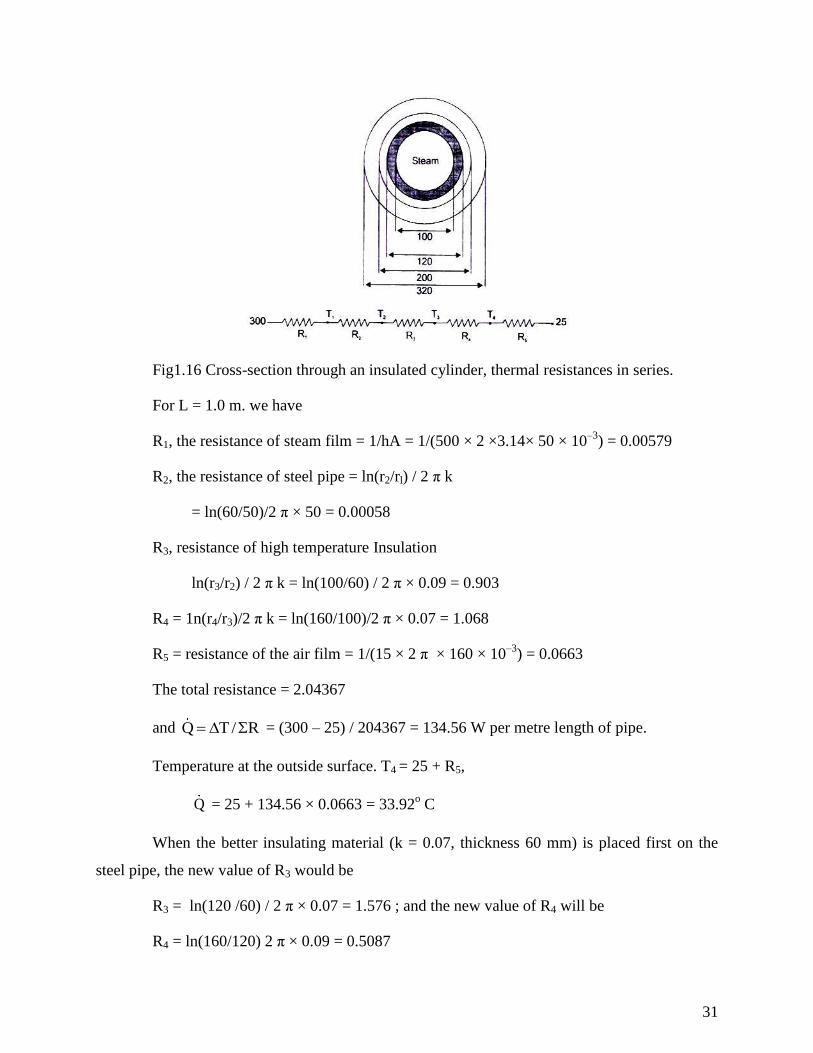
Solution: I he cross-section of the pipe with two layers of insulation is shown 111 Fig. 1.16. with

its analogous electrical circuit.

31

Fig1.16 Cross-section through an insulated cylinder, thermal resistances in series.

For L = 1.0 m. we have

R1, the resistance of steam film = 1/hA = 1/(500 × 2 ×3.14× 50 × 10–3

) = 0.00579

R2, the resistance of steel pipe = ln(r2/rl) / 2 π k

= ln(60/50)/2 π × 50 = 0.00058

R3, resistance of high temperature Insulation

ln(r3/r2) / 2 π k = ln(100/60) / 2 π × 0.09 = 0.903

R4 = 1n(r4/r3)/2 π k = ln(160/100)/2 π × 0.07 = 1.068

R5 = resistance of the air film = 1/(15 × 2 π × 160 × 10–3

) = 0.0663

The total resistance = 2.04367

and Q T / R = (300 – 25) / 204367 = 134.56 W per metre length of pipe.

Temperature at the outside surface. T4 = 25 + R5,

Q = 25 + 134.56 × 0.0663 = 33.92o C

When the better insulating material (k = 0.07, thickness 60 mm) is placed first on the

steel pipe, the new value of R3 would be

R3 = ln(120 /60) / 2 π × 0.07 = 1.576 ; and the new value of R4 will be

R4 = ln(160/120) 2 π × 0.09 = 0.5087

32

The total resistance = 2.15737 and Q = 275/2.15737 = 127.47 W per m length (Thus the

better insulating material be applied first to reduce the heat loss.) The overall heat transfer

coefficient, U, is obtained as U = Q / A T

The outer surface area = π × 320 × 10–3

× 1 = 1.0054

and U = 134.56/(275 × 1.0054) = 0.487 W/m2

K.

Example 1.13 A steam pipe 120 mm outside diameter and 10m long carries steam at a pressure

of 30 bar and 099 dry. Calculate the thickness of a lagging material (k = 0.99

W/mK) provided on the steam pipe such that the temperature at the outside

surface of the insulated pipe does not exceed 32°C when the steam flow rate is 1

kg/s and the dryness fraction of steam at the exit is 0.975 and there is no pressure

drop.

Solution: The latent heat of vaporization of steam at 30 bar = 1794 kJ/kg.

The loss of heat energy due to condensation of steam = 1794(0.99 – 0.975)

= 26.91 kJ/kg.

Since the steam flow rate is 1 kg/s, the loss of energy = 26.91 kW.

The saturation temperature of steam at 30 bar IS 233.84°C and assuming that the pipe

material offers negligible resistance to heat flow, the temperature at the outside surface of the

uninsulated steam pipe or at the inner surface of the lagging material is 233.84°C. Assuming

one-dimensional radial heat flow through the lagging material, we have

Q = (T1 – T2 )/[ln(r2/ rl)] 2 π Lk

or, 26.91 × 1000 (W) = (233.84 – 32) × 2 π × 10 × 0.99/1n(r/60)

ln (r/60) = 0.4666

r2/60 = exp (0.4666) = 1.5946

r2 = 95.68 mm and the thickness = 35.68 mm

Example 1.14 A Wire, diameter 0.5 mm length 30 cm, is laid coaxially in a tube (inside

diameter 1 cm, outside diameter 1.5 cm, k = 20 W/mK). The space between the

wire and the inside wall of the tube behaves like a hollow tube and is filled with a

33

gas. Calculate the thermal conductivity of the gas if the current flowing through

the wire is 5 amps and voltage across the two ends is 4.5 V, temperature of the

wire is 160°C, convective heat transfer coefficient at the outer surface of the tube

is 12 W/m2K and the ambient temperature is 300K.

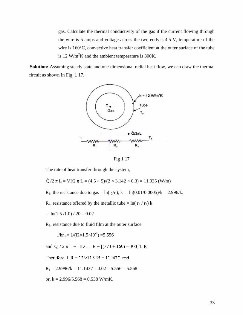
Solution: Assuming steady state and one-dimensional radial heat flow, we can draw the thermal

circuit as shown In Fig. 1 17.

Fig 1.17

The rate of heat transfer through the system,

Q /2 π L = VI/2 π L = (4.5 × 5)/(2 × 3.142 × 0.3) = 11.935 (W/m)

R1, the resistance due to gas = ln(r2/rl), k = ln(0.01/0.0005)/k = 2.996/k.

R2, resistance offered by the metallic tube = ln( r3 / r2) k

= ln(1.5 /1.0) / 20 = 0.02

R3, resistance due to fluid film at the outer surface

l/hr3 = 1/(l2×1.5×I0-2

) =5.556

and Q / 2 π –

R1 = 2.9996/k = 11.1437 – 0.02 – 5.556 = 5.568

or, k = 2.996/5.568 = 0.538 W/mK.

34

Example 1.15 A steam pipe (inner diameter 16 cm, outer diameter 20 cm, k = 50 W/mK) is

covered with a 4 cm thick insulating material (k = 0.09 W/mK). In order to

reduce the heat loss, the thickness of the insulation is Increased to 8mm.

Calculate the percentage reduction in heat transfer assuming that the convective

heat transfer coefficient at the Inside and outside surfaces are 1150 and 10

W/m2K and their values remain the same.

Solution: Assuming one-dimensional radial conduction under steady state,

Q / 2

R1, resistance due to steam film = 1/hr = 1/(1150 × 0.08) = 0.011

R2, resistance due to pipe material = ln (r2/r1)/k = ln (10/8)/50 = 0.00446

R3, resistance due to 4 cm thick insulation

= ln(r3/r2)/k = ln(14/10)/0.09 = 3.738

R4, resistance due to air film = 1/hr = 1/(10 × 0.14) = 0.714.

Therefore, Q/ 2 L T

When the thickness of the insulation is increased to 8 cm, the values of R3 and R4 will

change.

R3 = ln(r3/r2)/k = ln(18/10)/0.09 = 6.53 ; and

R4 = 1/hr = 1/(10 × 0.18) = 0.556

Therefore, Q/ 2 L T / (0.011 + 0.00446 + 6.53 + 0.556)

= T / 7.1 = 0.14084 T

Percentage reduction in heat transfer = 0.22386 0.14084

0.37 37%0.22386

Example 1.16 A small hemispherical oven is built of an inner layer of insulating fire brick 125

mm thick (k = 0.31 W/mK) and an outer covering of 85% magnesia 40 mm thick (k

= 0.05 W/mK). The inner surface of the oven is at 1073 K and the heat transfer

coefficient for the outer surface is 10 W/m2K, the room temperature is 20

oC.

35

Calculate the rate of heat loss through the hemisphere if the inside radius is 0.6 m.

Solution: The resistance of the fire brick

= 2 1 1 2

0.725 0.6r r / 2 kr r 0.1478

2 0.31 0.6 0.725

The resistance of 85% magnesia

= 3 2 2 3

0.765 0.725r r / 2 kr r 0.2295

2 0.05 0.725 0.765

The resistance due to fluid film at the outer surface = 1/hA

10.2295

10 2 0.765 0.765

The resistance due to fluid film at the outer surface = 1/hA

10.0272

10 2 0.765 0.765

Rate of heat flow, 800 20

Q T / R 1930W0.1478 0.2295 0.272

Example 1.17 A cylindrical tank with hemispherical ends is used to store liquid oxygen at –

180oC. The diameter of the tank is 1.5 m and the total length is 8 m. The tank is

covered with a 10 cm thick layer of insulation. Determine the thermal conductivity

of the insulating material so that the boil off rate does not exceed 10 kg/hr. The

latent heat of vapourization of liquid oxygen is 214 kJ/kg. Assume that the outer

surface of insulation is at 27oC and the thermal resistance of the wall of the tank is

negligible. (ES-94)

Solution: The maximum amount of heat energy that flows by conduction from outside

to inside = Mass of liquid oxygen × Latent heat of vapourisation.

= 10 × 214 = 2140 kJ/hr = 2140 × 1000/3600 = 594.44 W

Length of the cylindrical part of the tank = 8 – 2r = 8 – 1.5 = 6.5m

since the thermal resistance of the wall does not offer any resistance to heat flow, the

temperature at the inside surface of the insulation can be assumed as - 183°C whereas the

36

temperature at the outside surface of the insulation is 27°C.

Heat energy coming in through the cylindrical part, 1

2 1

TQ

ln r / r

2 Lk

or,

1

27 183 2 6.5kQ 68531.84 k

ln 8.5 / 7.5

Heat energy coming in through the two hemispherical ends,

2 2 1 2 1

2 210 2 k 0.85 0.75Q 2 T 2 k r r / r r

0.10

= 16825.4 k

Therefore, 594.44 = (68531.84 + 16825.4) k; or, k = 6.96 × 10–3

W/mK.

Example 1.18 A spherical vessel, made out of2.5 em thick steel plate IS used to store

10m3 of a liquid at 200°C for a thermal storage system. To reduce the heat loss to the

surroundings, a 10 cm thick layer of insulation (k = 0.07 W/rnK) is used. If the convective heat

transfer coefficient at the outer surface is W/m2K and the ambient temperature is 25°C, calculate

the rate of heat loss neglecting the thermal resistance of the steel plate.

If the spherical vessel is replaced by a 2 m diameter cylindrical vessel with flat ends,

calculate the thickness of insulation required for the same heat loss.

Solution: Volume of the spherical vessel = 3

3 4 r10m

3

r 1.336 m

Outer radius of the spherical vessle, 2r 1.3364 0.025 1.361 m

Outermost radius of the spherical vessel after the insulation = 1.461 m.

Since the thermal resistance of the steel plate is negligible, the temperature at the inside

surface of the insulation is 200oC.

Thermal resistance of the insulating material = 3 2 3 2r r / 4 k r r

0.1

0.0574 0.07 1.461 1.361

Thermal resistance of the fluid film at the outermost surface = 1/hA

37

2

1/ 10 4 1.461 0.00373

Rate of heat flow = T / R 200 25 / 0.057 0.00373 2873.8 W

Volume of the insulating material used = 3 3 33 24 / 3 r r 2.5 m

Volume of the cylindrical vessel 2310 m d L; L 10 / 3.183m

4

Outer radius of cylinder without insulation = 1.0 + 0.025 = 1.025 m.

Outermost radius of the cylinder (with insulation) = r3.

Therefore, the thickness of insulation = r3 – 1.025 =

Resistance, the heat flow by the cylindrical element

3 3

3

ln r /1.025 ln r /1.025 11/ hA

2 Lk 2 3.183 0.07 10 2 r 3.183

= 0.714 ln (r3 / 1.025) + 0.005/r3

Resistance to heat flow through sides of the cylinder

32 r 1.025 1

2 / kA 1/ hA0.07 1 10 2

39.09 r 1.025 0.0159

For the same heat loss, T / R would be equal in both cases, therefore,

3 3 3

1 1 1

0.06073 0.714 ln r /1.025 0.005 / r 9.09 r 1.025 0.0159

Solving by trial and error, (r –

and the volume of the insulating material required = 2.692 m3.

7. Unsteady State Conduction Heat Transfer

7.1 . Transient State Systems-Defined

38

The process of heat transfer by conduction where the temperature varies with time and

with space coordinates, is called 'unsteady or transient'. All transient state systems may be

broadly classified into two categories:

(a) Non-periodic Heat Flow System - the temperature at any point within the system

changes as a non-linear function of time.

(b) Periodic Heat Flow System - the temperature within the system undergoes periodic

changes which may be regular or irregular but definitely cyclic.

There are numerous problems where changes in conditions result in transient

temperature distributions and they are quite significant. Such conditions are encountered in -

manufacture of ceramics, bricks, glass and heat flow to boiler tubes, metal forming, heat

treatment, etc.

7.2. Biot and Fourier Modulus-Definition and Significance

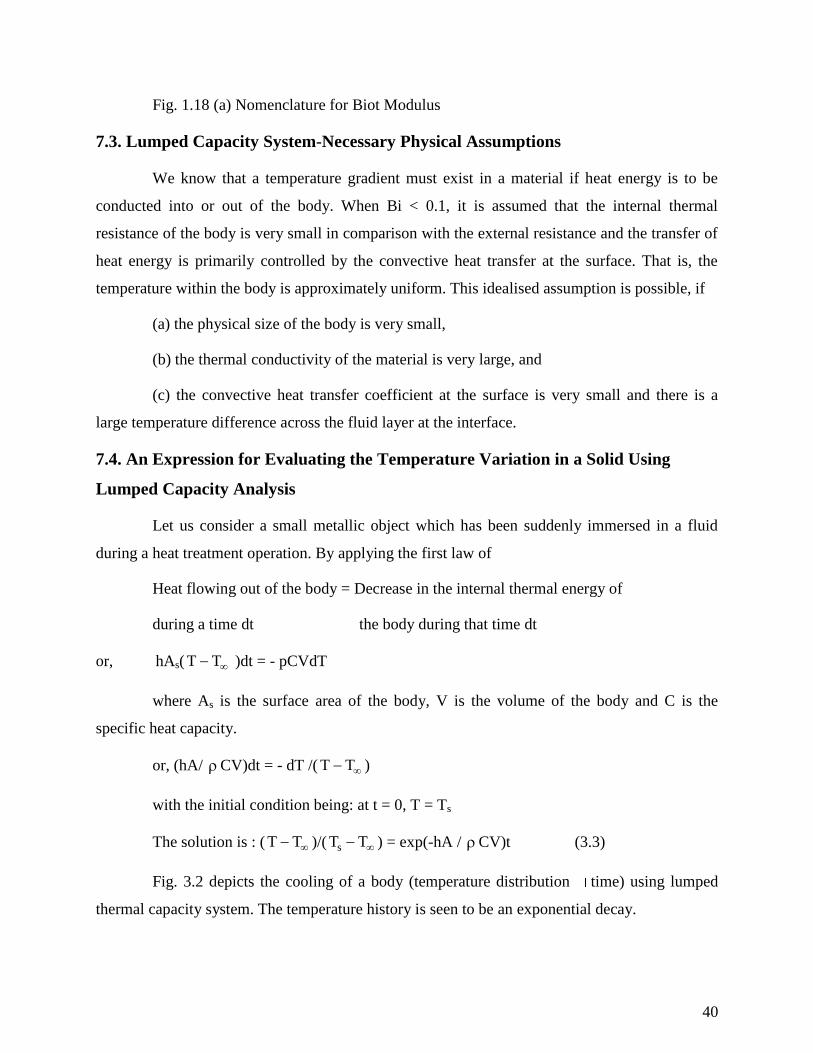
Let us consider an initially heated long cylinder (L >> R) placed in a moving stream of

fluid at sT T , as shown In Fig. 3.1(a). The convective heat transfer coefficient at the surface is

h, where,

Q = hA ( sT T )

This energy must be conducted to the surface, and therefore,

Q = -kA(dT / dr) r = R

or, h( sT T ) = -k(dT/dr)r=R -k(Tc-Ts)/R

where Tc is the temperature at the axis of the cylinder

By rearranging,(Ts - Tc) / ( sT T ) h/Rk (3.1)

The term, hR/k, IS called the 'BlOT MODULUS'. It is a dimensionless number and is

the ratio of internal heat flow resistance to external heat flow resistance and plays a fundamental

role in transient conduction problems involving surface convection effects. I t provides a

measure 0 f the temperature drop in the solid relative to the temperature difference between the

surface and the fluid.

39

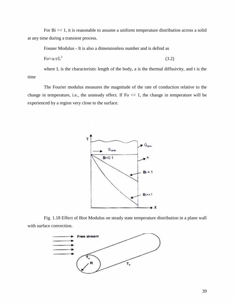
For Bi << 1, it is reasonable to assume a uniform temperature distribution across a solid

at any time during a transient process.

Founer Modulus - It is also a dimensionless number and is defind as

Fo= t/L2

(3.2)

where L is the characteristic length of the body, a is the thermal diffusivity, and t is the

time

The Fourier modulus measures the magnitude of the rate of conduction relative to the

change in temperature, i.e., the unsteady effect. If Fo << 1, the change in temperature will be

experienced by a region very close to the surface.

Fig. 1.18 Effect of Biot Modulus on steady state temperature distribution in a plane wall

with surface convection.

40

Fig. 1.18 (a) Nomenclature for Biot Modulus

7.3. Lumped Capacity System-Necessary Physical Assumptions

We know that a temperature gradient must exist in a material if heat energy is to be

conducted into or out of the body. When Bi < 0.1, it is assumed that the internal thermal

resistance of the body is very small in comparison with the external resistance and the transfer of

heat energy is primarily controlled by the convective heat transfer at the surface. That is, the

temperature within the body is approximately uniform. This idealised assumption is possible, if

(a) the physical size of the body is very small,

(b) the thermal conductivity of the material is very large, and

(c) the convective heat transfer coefficient at the surface is very small and there is a

large temperature difference across the fluid layer at the interface.

7.4. An Expression for Evaluating the Temperature Variation in a Solid Using

Lumped Capacity Analysis

Let us consider a small metallic object which has been suddenly immersed in a fluid

during a heat treatment operation. By applying the first law of

Heat flowing out of the body = Decrease in the internal thermal energy of

during a time dt the body during that time dt

or, hAs( T T )dt = - pCVdT

where As is the surface area of the body, V is the volume of the body and C is the

specific heat capacity.

or, (hA/ CV)dt = - dT /( T T )

with the initial condition being: at t = 0, T = Ts

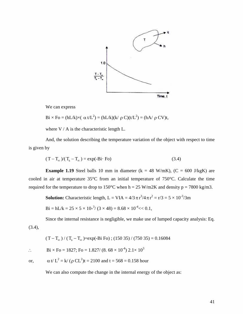
The solution is : ( T T )/( sT T ) = exp(-hA / CV)t (3.3)

Fig. 3.2 depicts the cooling of a body (temperature distribution time) using lumped

thermal capacity system. The temperature history is seen to be an exponential decay.

41

We can express

Bi × Fo = (hL/k)×( t/L2) = (hL/k)(k/ C)(t/L

2) = (hA/ CV)t,

where V / A is the characteristic length L.

And, the solution describing the temperature variation of the object with respect to time

is given by

( T T )/( sT T ) = exp(-Bi· Fo) (3.4)

Example 1.19 Steel balls 10 mm in diameter (k = 48 W/mK), (C = 600 J/kgK) are

cooled in air at temperature 35°C from an initial temperature of 750°C. Calculate the time

required for the temperature to drop to 150°C when h = 25 W/m2K and density p = 7800 kg/m3.

Solution: Characteristic length, L = VIA = 4/3 r3/4 r

2 = r/3 = 5 × 10

-3/3m

Bi = hL/k = 25 × 5 × 10-3/ (3 × 48) = 8.68 × 10

-4<< 0.1,

Since the internal resistance is negligible, we make use of lumped capacity analysis: Eq.

(3.4),

( T T ) / ( sT T )=exp(-Bi Fo) ; (150 35) / (750 35) = 0.16084

Bi × Fo = 1827; Fo = 1.827/ (8. 68 × 10-4

) 2.1× 103

or, t/ L2 = k/ (CL

2)t = 2100 and t = 568 = 0.158 hour

We can also compute the change in the internal energy of the object as:

42

1 1

0 t s0 0U U CVdT CV T T hA / CV exp t hAt / CV dt

= sCV T T exp hAt / CV 1 (3.5)

= -7800 × 600 × (4/3) (5 × 10-3

)3 (750-35) (0.16084 - 1)

= 1.47 × 103 J = 1.47 kJ.

If we allow the time 't' to go to infinity, we would have a situation that corresponds to

steady state in the new environment. The change in internal energy will be U0 - U =

[CV( sT T ) exp(- )- 1] = [CV( sT T ].

We can also compute the instantaneous heal transfer rate at any time.

or. Q = -VCdT/dt = -VCd/dt[ T + ( sT T )exp(-hAt/CV) ]

= hA( sT T )[exp(-hAt/ CV)) and for t = 60s,

Q = 25 × 4 × 3.142 (5 × 10-3

)2(750 35) [exp( -25 × 3 × 60/5 × 10

-3 × 7800 × 600)]

= 4.63 W.

Example 1.20 A cylindrical steel ingot (diameter 10 cm. length 30 cm, k = 40 W mK.

= 7600 kg/m3, C = 600 J/kgK) is to be heated in a furnace from 50°C to 850°C. The

temperature inside the furnace is 1300oC and the surface heat transfer coefficient is 100 W/m

2K.

Calculate the time required.

Solution: Characteristic length. L = V/A = r2L/2 r(r+ L) = rL/2(r + L)

= 5 × 10-2

× 30 × 10-2

/2 (2 (5 +30) × 10-2

)

= 2.143 × 10-2

m.

Bi = hL/k = 100 × 2.143 × 10-2

/40 = 0.0536 << 0.1

Fo = t/L2 = (k/C) × (t/L

2)

= 40 × t/(7600 × 600 × [2.143 × 1 0-2

)2] = 191 × 10

-2 t

and ( T T )/( sT T ) = exp(-Bi Fo)

or, (850 - 1300) /(50 - 1300) = 0.36 = exp (- Bi Fo)

43

Bi Fo= 102

and Fo = 19.06 and t = 19.06/( 1.91 × 1 0 -2

) = 16.63 min

(The length of the ingot is 30 cm and it must be removed from the furnace after a period

of 16.63 min. therefore, the speed of the ingot would be 0.3/16.63 = 1.8 × 10-2

m/min.)

Example 1.21 A block of aluminium (2cm × 3cm × 4cm, k = 180 W/mK, = 10 -4

m2/s)

inllially at 300oC is cooled in air at 30

oC. Calculate the temperature of the block after 3 min.

Take h = 50W/ m2K.

Solution: Characteristic length, L= [2 × 3 × 4 /2(2 × 3 + 2 × 4 + 3 × 4)] × 10-2

= 4.6 × 10-3

m

Bi = hL/k = 50 × 4.6 × 10-3

/180 = 1.278 × 10-3

<< 0.1

Fo = t/L2 =10

-4 × 180 / (4.6×10

-3)2 = 850

exp(-Bi Fo) = exp(-1.278 × 10-3

×'850) = 0.337

(T - T ) (Ts - T ) - (T - 30)/(300 - 30) = 0.337

T= 121.1°C.

Example 1.22 A copper wire 1 mm in diameter initially at 150°C is suddenly dipped

into water at 35°C. Calculate the time required to cool to a temperature of 90°C if h = 100 W/

m2K. What would be the time required if h = 40 W/m

2K. (for copper; k = 370 W/mK, = 8800

kg/m3. C = 381 J/kgK.

Solution: The characteristic length for a long cylindrical object can be approximated as

r/2. As such,

Bi = hL/k = 100 × 0.5 × 10 -3

/ (2 × 370) = 6.76 × 10-5

<< 0.1

Fo = t/L2 = (k/ C ) × (t/L

2)

= [370t/(8800 × 381 × (0.25 × 10-3

)2] = 1760t

exp(-Bi Fo) = (T - T )(Ts -T )

= (90 - 35)/(150 - 35) = 0.478

44

Bi Fo = 0.738 = 6.76 × 10-5

× 1760 t; t = 6.2s

when h = 40 W/ m2K, Bi = 2.7 × 10

-5 and 2.7 × 10

-5 ×1760 t = 0.738;

or, t = 15.53s.

Example 1.23 A metallic rod (mass 0.1 kg, C = 350 J/kgK, diameter 12.5 mm, surface

area 40cm2) is initially at 100°C. It is cooled in air at 25°C. If the temperature drops to 40°C in

100 seconds, estimate the surface heat transfer coefficient.

Solution: hA/ CV = hA/ mC = h × 40 × 10-4

/(0.1 × 350) = 1.143×10-4

h

and, hAt / CV = 1.143 × 10-4

h × 100 = 1.143 × 10 -2

h

(T - T )/(Ts - T ) = (40 - 25) / (100 - 25) = 0.2

exp( -1.143 × 10-2

h) = 0.2

or, 1.143 × 10-2

h = 1.6094, and h = 140W/m2K.

45

SCHOOL OF MECHANICAL

DEPARTMENT OF MECHANICAL

UNIT – II – Heat and Mass Transfer– SMEA1504

46

UNIT – 2

CONVECTION

2.1. Convection Heat Transfer-Requirements

The heat transfer by convection requires a solid-fluid interface, a temperature difference

between the solid surface and the surrounding fluid and a motion of the fluid. The process of heat

transfer by convection would occur when there is a movement of macro-particles of the fluid in

space from a region of higher temperature to lower temperature.

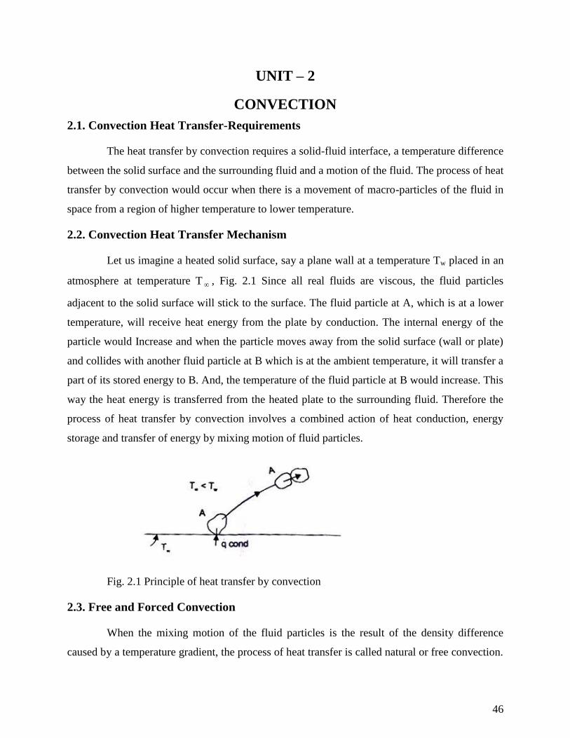
2.2. Convection Heat Transfer Mechanism

Let us imagine a heated solid surface, say a plane wall at a temperature Tw placed in an

atmosphere at temperature T , Fig. 2.1 Since all real fluids are viscous, the fluid particles

adjacent to the solid surface will stick to the surface. The fluid particle at A, which is at a lower

temperature, will receive heat energy from the plate by conduction. The internal energy of the

particle would Increase and when the particle moves away from the solid surface (wall or plate)

and collides with another fluid particle at B which is at the ambient temperature, it will transfer a

part of its stored energy to B. And, the temperature of the fluid particle at B would increase. This

way the heat energy is transferred from the heated plate to the surrounding fluid. Therefore the

process of heat transfer by convection involves a combined action of heat conduction, energy

storage and transfer of energy by mixing motion of fluid particles.

Fig. 2.1 Principle of heat transfer by convection

2.3. Free and Forced Convection

When the mixing motion of the fluid particles is the result of the density difference

caused by a temperature gradient, the process of heat transfer is called natural or free convection.

47

When the mixing motion is created by an artificial means (by some external agent), the process

of heat transfer is called forced convection Since the effectiveness of heat transfer by convection

depends largely on the mixing motion of the fluid particles, it is essential to have a knowledge of

the characteristics of fluid flow.

2.4. Basic Difference between Laminar and Turbulent Flow

In laminar or streamline flow, the fluid particles move in layers such that each fluid p

article follows a smooth and continuous path. There is no macroscopic mixing of fluid particles

between successive layers, and the order is maintained even when there is a turn around a comer

or an obstacle is to be crossed. If a lime dependent fluctuating motion is observed indirections

which are parallel and transverse to the main flow, i.e., there is a random macroscopic mixing of

fluid particles across successive layers of fluid flow, the motion of the fluid is called' turbulent

flow'. The path of a fluid particle would then be zigzag and irregular, but on a statistical basis,

the overall motion of the macro particles would be regular and predictable.

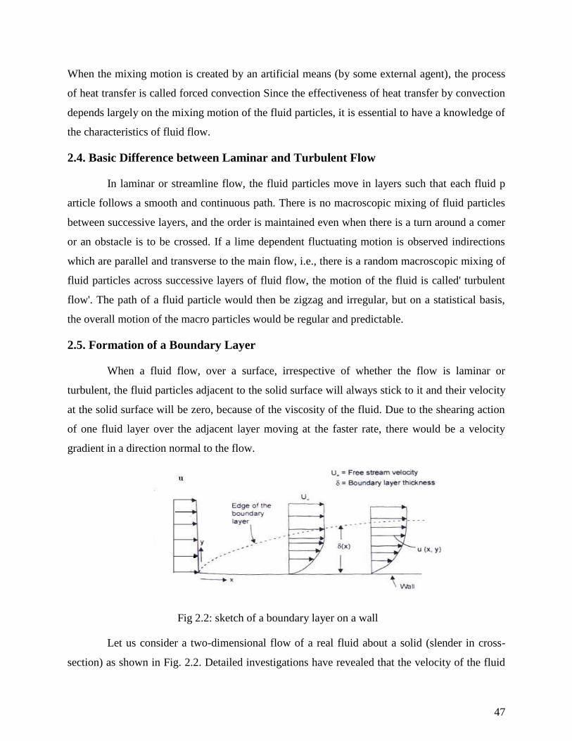
2.5. Formation of a Boundary Layer

When a fluid flow, over a surface, irrespective of whether the flow is laminar or

turbulent, the fluid particles adjacent to the solid surface will always stick to it and their velocity

at the solid surface will be zero, because of the viscosity of the fluid. Due to the shearing action

of one fluid layer over the adjacent layer moving at the faster rate, there would be a velocity

gradient in a direction normal to the flow.

Fig 2.2: sketch of a boundary layer on a wall

Let us consider a two-dimensional flow of a real fluid about a solid (slender in cross-

section) as shown in Fig. 2.2. Detailed investigations have revealed that the velocity of the fluid

48

particles at the surface of the solid is zero. The transition from zero velocity at the surface of the

solid to the free stream velocity at some distance away from the solid surface in the V-direction

(normal to the direction of flow) takes place in a very thin layer called 'momentum or

hydrodynamic boundary layer'. The flow field can thus be divided in two regions:

( i) A very thin layer in t he vicinity 0 f t he body w here a velocity gradient normal to

the direction of flow exists, the velocity gradient du/dy being large. In this thin region, even a

very small Viscosity of the fluid exerts a substantial Influence and the shearing stress

du/dy may assume large values. The thickness of the boundary layer is very small and

decreases with decreasing viscosity.

(ii) In the remaining region, no such large velocity gradients exist and the Influence of

viscosity is unimportant. The flow can be considered frictionless and potential.

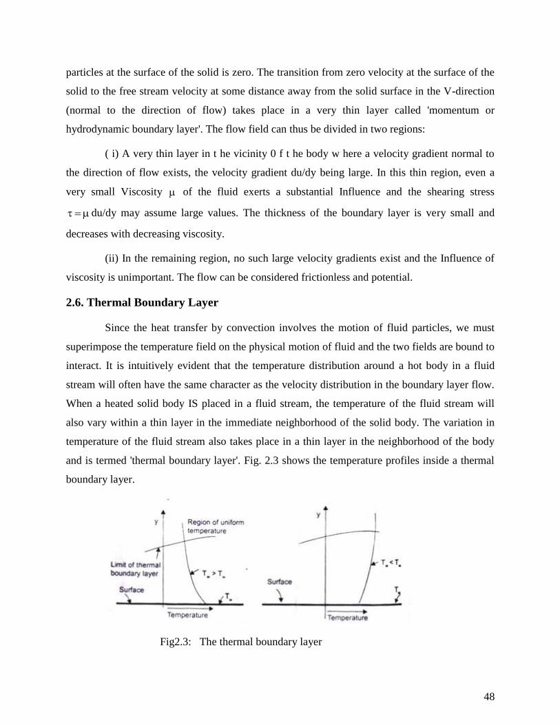
2.6. Thermal Boundary Layer

Since the heat transfer by convection involves the motion of fluid particles, we must

superimpose the temperature field on the physical motion of fluid and the two fields are bound to

interact. It is intuitively evident that the temperature distribution around a hot body in a fluid

stream will often have the same character as the velocity distribution in the boundary layer flow.

When a heated solid body IS placed in a fluid stream, the temperature of the fluid stream will

also vary within a thin layer in the immediate neighborhood of the solid body. The variation in

temperature of the fluid stream also takes place in a thin layer in the neighborhood of the body

and is termed 'thermal boundary layer'. Fig. 2.3 shows the temperature profiles inside a thermal

boundary layer.

Fig2.3: The thermal boundary layer

49

2.7. Dimensionless Parameters and their Significance

The following dimensionless parameters are significant in evaluating the convection

heat transfer coefficient:

(a) The Nusselt Number (Nu)-It is a dimensionless quantity defined as hL/ k, where h =

convective heat transfer coefficient, L is the characteristic length and k is the thermal

conductivity of the fluid The Nusselt number could be interpreted physically as the ratio of the

temperature gradient in the fluid immediately in contact with the surface to a reference

temperature gradient (Ts - T ) /L. The convective heat transfer coefficient can easily be obtained

if the Nusselt number, the thermal conductivity of the fluid in that temperature range and the

characteristic dimension of the object is known.

Let us consider a hot flat plate (temperature Tw) placed in a free stream (temperature

T < Tw). The temperature distribution is shown ill Fig. 2.4. Newton's Law of Cooling says that

the rate of heat transfer per unit area by convection is given by

wQ / A h T T

w

Qh(T T )

A

= w

t

T Tk

h = t

k

Nu = t

hL L

k

50

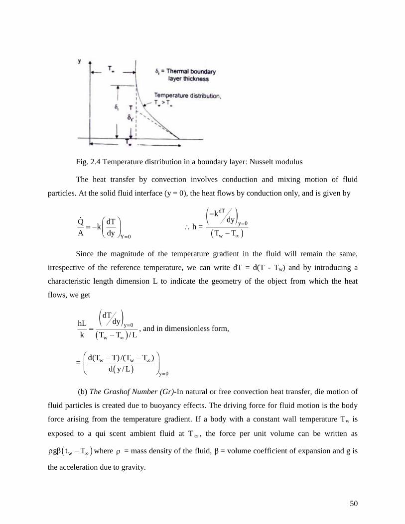
Fig. 2.4 Temperature distribution in a boundary layer: Nusselt modulus

The heat transfer by convection involves conduction and mixing motion of fluid

particles. At the solid fluid interface (y = 0), the heat flows by conduction only, and is given by

Y 0

Q dTk

A dy

h =

dT

y 0

w

kdy

T T

Since the magnitude of the temperature gradient in the fluid will remain the same,

irrespective of the reference temperature, we can write dT = d(T - Tw) and by introducing a

characteristic length dimension L to indicate the geometry of the object from which the heat

flows, we get

y 0

w

dTdyhL

k T T / L

, and in dimensionless form,

=

w w

y 0

d(T T) /(T T )

d y / L

(b) The Grashof Number (Gr)-In natural or free convection heat transfer, die motion of

fluid particles is created due to buoyancy effects. The driving force for fluid motion is the body

force arising from the temperature gradient. If a body with a constant wall temperature Tw is

exposed to a qui scent ambient fluid at T , the force per unit volume can be written as

wg t T where = mass density of the fluid, = volume coefficient of expansion and g is

the acceleration due to gravity.

51

The ratio of inertia force × Buoyancy force/(viscous force)2 can be written as

2 2 3w

2

V L g T T LGr

VL

=

2 3

w 3 2w2

g T T Lg L T T /

The magnitude of Grashof number indicates whether the flow is laminar or turbulent. If

the Grashof number is greater than 109, the flow is turbulent and for Grashof number less than

108, the flow is laminar. For 10

8 < Gr < 10

9, It is the transition range.

(c) The Prandtl Number (Pr) - It is a dimensionless parameter defined as

Pr = pC / k /

Where is the dynamic viscosity of the fluid, v = kinematic viscosity and = thermal

diffusivity.

This number assumes significance when both momentum and energy are propagated

through the system. It is a physical parameter depending upon the properties of the medium It is

a measure of the relative magnitudes of momentum and thermal diffusion in the fluid: That is,

for Pr = I, the r ate of diffusion of momentum and energy are equal which means that t he

calculated temperature and velocity fields will be Similar, the thickness of the momentum and

thermal boundary layers will be equal. For Pr <<I (in case of liquid metals), the thickness of the

thermal boundary layer will be much more than the thickness of the momentum boundary layer

and vice versa. The product of Grashof and Prandtl number is called Rayleigh number. Or, Ra =

Gr × Pr.

2.8. Evaluation of Convective Heat Transfer Coefficient

The convective heat transfer coefficient in free or natural convection can be evaluated

by two methods:

(a) Dimensional Analysis combined with experimental investigations

(b) Analytical solution of momentum and energy equations 10 the boundary layer.

Dimensional Analysis and Its Limitations

52

Since the evaluation of convective heat transfer coefficient is quite complex, it is based

on a combination of physical analysis and experimental studies. Experimental observations

become necessary to study the influence of pertinent variables on the physical phenomena.

Dimensional analysis is a mathematical technique used in reducing the number of

experiments to a minimum by determining an empirical relation connecting the relevant

variables and in grouping the variables together in terms of dimensionless numbers. And, the

method can only be applied after the pertinent variables controlling t he phenomenon are

Identified and expressed In terms of the primary dimensions. (Table 1.1)

In natural convection heat transfer, the pertinent variables are: h, , k, , Cp, L, (T),

and g. Buckingham 's method provides a systematic technique for arranging the variables in

dimensionless numbers. It states that the number of dimensionless groups, ’s, required to

describe a phenomenon involving 'n' variables is equal to the number of variables minus the

number of primary dimensions 'm' in the problem.

In SI system of units, the number of primary dimensions are 4 and the number of

variables for free convection heat transfer phenomenon are 9 and therefore, we should expect (9 -

4) = 5 dimensionless numbers. Since the dimension of the coefficient of volume expansion, , is

1 , one dimensionless number is obviously (T). The remaining variables are written in a

functional form:

ph, ,k, ,C ,L,g = 0.

Since the number of primary dimensions is 4, we arbitrarily choose 4 independent

variables as primary variables such that all the four dimensions are represented. The selected

primary variables are: ,g, k. L Thus the dimensionless group,

a b

a b c d 3 2 3 1 0 0 0 01 g k L h ML LT . MLT M L T

Equating the powers of M, L, T, on both sides, we have

53

M : a + c + 1 = 0 } Upon solving them,

L : -3a + b + c + d = 0

T : -2b -3c -3 = 0

: -c - 1 = 0

Up on solving them,

c = 1, b = a = 0 and d = 1.

and 1 = hL/k, the Nusselt number.

The other dimensionless number

2= pag

bk

cL

dCp = (ML

-3)a (LT

-2)b(MLT

-3

-1)c(L)

d(MT

-1 1 ) = M0L

0T

0

0 Equating the

powers of M,L,T and and upon solving, we get

3= 2 2 3/ g L

By combining 2 and 3 , we write 1/ 2

4 2 3

= 1/ 2

2 3 2 2 2 3pgL C / k / gL

=

pC

k

(the Prandtl number)

By combining 3 with T , we have 5= T *3

1

= 2 3

3 2

2

gLT g T L /

(the Grashof number)

Therefore, the functional relationship is expressed as:

m

1Nu,Pr,Gr 0;Or, Nu Gr Pr Const Gr Pr (2.1)

and values of the constant and 'm' are determined experimentally.

Table 2.1 gives the values of constants for use with Eq. (2.1) for isothermal surfaces.

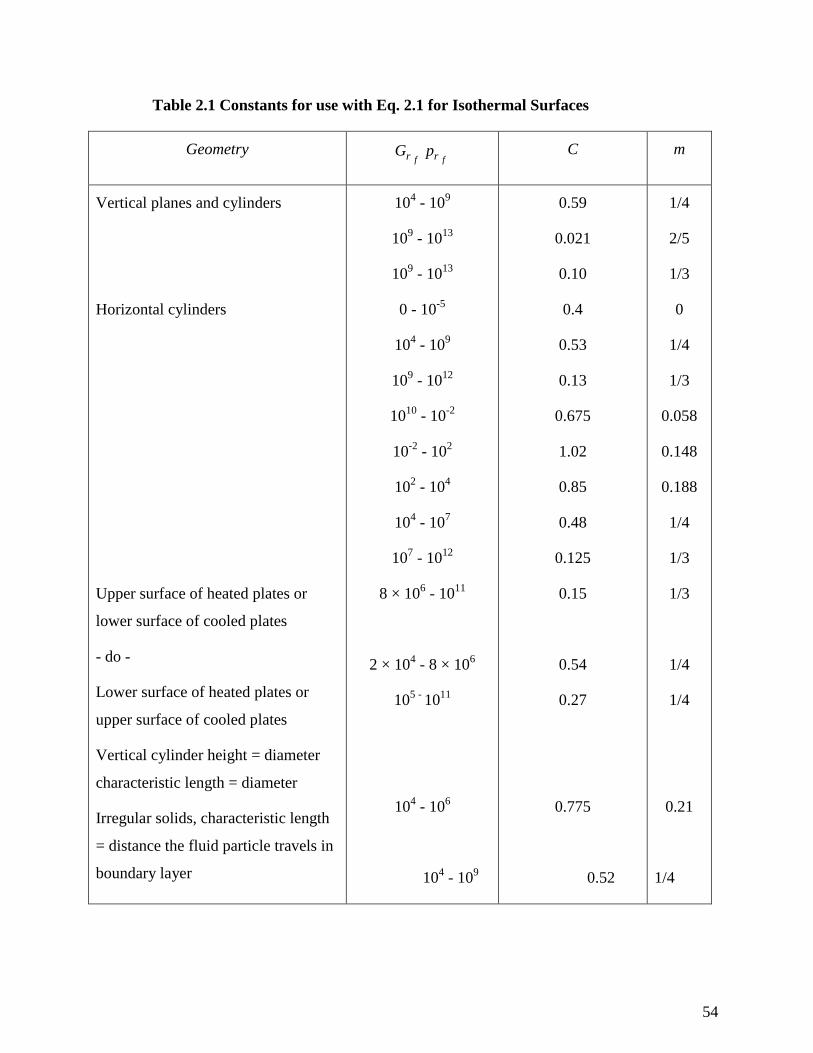
54

Table 2.1 Constants for use with Eq. 2.1 for Isothermal Surfaces

Geometry f fr rG p C m

Vertical planes and cylinders

Horizontal cylinders

Upper surface of heated plates or

lower surface of cooled plates

- do -

Lower surface of heated plates or

upper surface of cooled plates

Vertical cylinder height = diameter

characteristic length = diameter

Irregular solids, characteristic length

= distance the fluid particle travels in

boundary layer

104 - 10

9

109 - 10

13

109 - 10

13

0 - 10-5

104 - 10

9

109 - 10

12

1010

- 10-2

10-2

- 102

102 - 10

4

104 - 10

7

107 - 10

12

8 × 106 - 10

11

2 × 104 - 8 × 10

6

105 -

1011

104 - 10

6

104 - 10

9

0.59

0.021

0.10

0.4

0.53

0.13

0.675

1.02

0.85

0.48

0.125

0.15

0.54

0.27

0.775

0.52

1/4

2/5

1/3

0

1/4

1/3

0.058

0.148

0.188

1/4

1/3

1/3

1/4

1/4

0.21

1/4

55

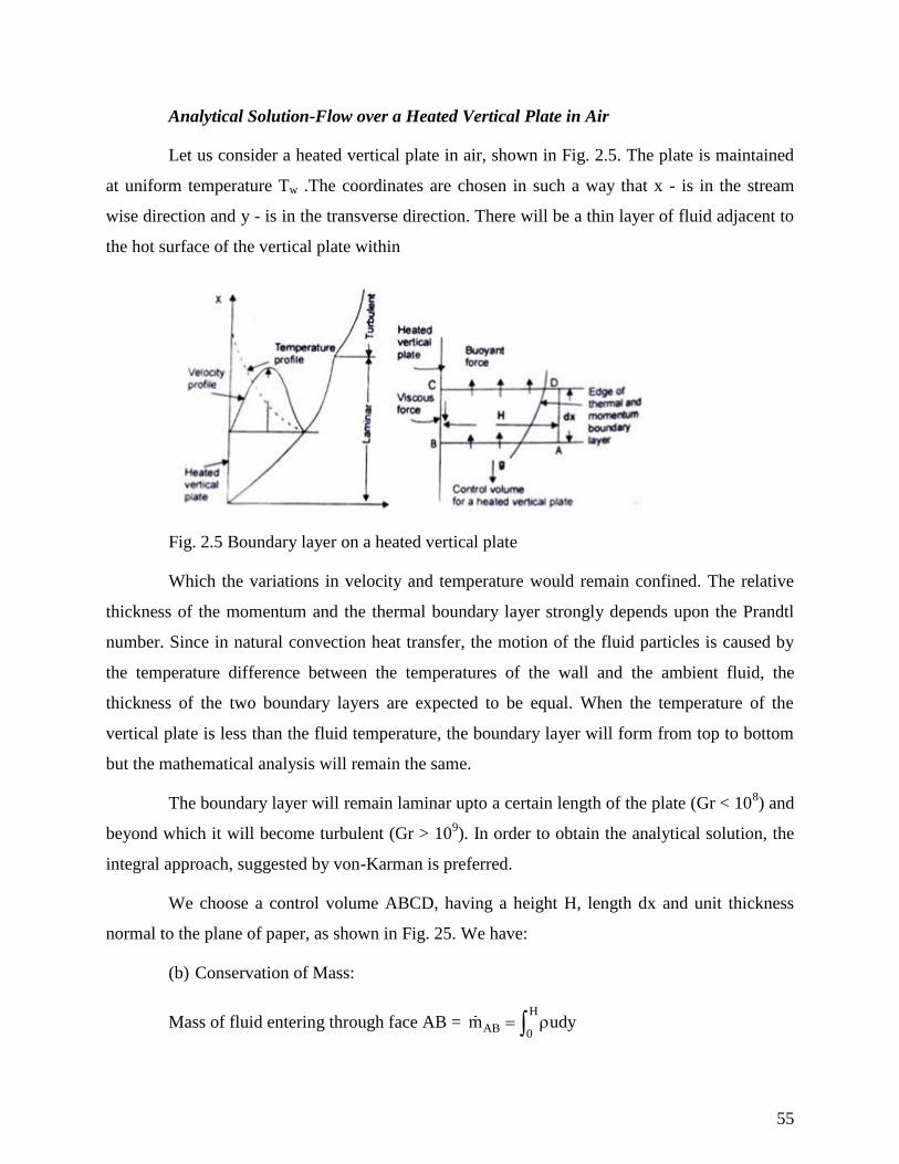
Analytical Solution-Flow over a Heated Vertical Plate in Air

Let us consider a heated vertical plate in air, shown in Fig. 2.5. The plate is maintained

at uniform temperature Tw .The coordinates are chosen in such a way that x - is in the stream

wise direction and y - is in the transverse direction. There will be a thin layer of fluid adjacent to

the hot surface of the vertical plate within

Fig. 2.5 Boundary layer on a heated vertical plate

Which the variations in velocity and temperature would remain confined. The relative

thickness of the momentum and the thermal boundary layer strongly depends upon the Prandtl

number. Since in natural convection heat transfer, the motion of the fluid particles is caused by

the temperature difference between the temperatures of the wall and the ambient fluid, the

thickness of the two boundary layers are expected to be equal. When the temperature of the

vertical plate is less than the fluid temperature, the boundary layer will form from top to bottom

but the mathematical analysis will remain the same.

The boundary layer will remain laminar upto a certain length of the plate (Gr < 108) and

beyond which it will become turbulent (Gr > 109). In order to obtain the analytical solution, the

integral approach, suggested by von-Karman is preferred.

We choose a control volume ABCD, having a height H, length dx and unit thickness

normal to the plane of paper, as shown in Fig. 25. We have:

(b) Conservation of Mass:

Mass of fluid entering through face AB = H

AB 0m udy

56

Mass of fluid leaving face CD = H H

CD 0 0

dm udy udy dx

dx

Mass of fluid entering the face DA = H

0

dudy dx

dx

(ii) Conservation of Momentum:

Momentum entering face AB = H 2

0u dy

Momentum leaving face CD = H H2 2

0 0

du dy u dy dx

dx

Net efflux of momentum in the + x-direction = H 2

0

du dy dx

dx

The external forces acting on the control volume are:

(a) Viscous force =

y 0

dudx

dy

acting in the –ve x-direction

(b) Buoyant force approximated as H

0g T T dy dx

From Newton’s law, the equation of motion can be written as:

2

0 0y 0

d duu dy g T T dy

dx dy

(2.2)

because the value of the integrand between and H would be zero.

(iii) Conservation of Energy:

ABQ , convection + ADQ ,convection + BCQ ,conduction = CDQ convection

or, H H

0 0y 0

d dTuCTdy CT udy dx k dx

dx dy

= H H

0 0

duCTdy uTCdy dx

dx

57

or 0

y 0 y 0

d k dT dTu T T dy

dx C dy dy

(2.3)

The boundary conditions are:

or,

(2.3)

Velocity profile Temperature profile

u = 0 at y = 0 T = Tw at y = 0

u = 0 at y = T = Tat y = 1

du/dy = 0 at y = dT/dy 0 at y = 1

Since the equations (2.2) and (2.3) are coupled equations, it is essential that the

functional form of both the velocity and temperature distribution are known in order to arrive at a

solution.

The functional relationships for velocity and temperature profiles which satisfy the

above boundary conditions are assumed of the form:

2

*

u y y1

u

(2.4)

Where *u is a fictitious velocity which is a function of x; and

2

w

T T y1

T T

(2.5)

After the Eqs. (5.4) and (5.5) are inserted in Eqs. (5.2) and (5.3) and the operations are

performed (details of the solution are given in Chapman, A.J. Heat Transfer, Macmillan

Company, New York), we get the expression for boundary layer thickness as:

0.250.5 0.25

x/ x 3.93Pr 0.952 Pr Gr

Where Gr, is the local Grashof number = 3 2wg x T T /

58

The heat transfer coefficient can be evaluated from:

w w

y 0

dTq k h T T

dy

Using Eq. (5.5) which gives the temperature distribution, we have

h = 2k/ or, hx/k = Nux= 2x/

The non-dimensional equation for the heat transfer coefficient is

Nux= 0.508 Pr0.5

(0.952 + Pr)-0.25 0.25

xGr (2.7)

The average heat transfer coefficient, L

x x L0

1h h dx 4/3h

L

NuL= 0.677 Pr0.5

(0.952 + Pr)-0.25 0.25Gr (2.8)

Limitations of Analytical Solution: Except for the analytical solution for flow over a flat

plate, experimental measurements are required to evaluate the heat transfer coefficient. Since in

free convection systems, the velocity at the surface of the wall and at the edge of the boundary

layer is zero and its magnitude within the boundary layer is so small. It is very difficult to

measure them. Therefore, velocity measurements require hydrogen-bubble technique or sensitive

hot wire anemometers. The temperature field measurement is obtained by interferometer.

Expression for ‘h’ for a Heated Vertical Cylinder in Air

The characteristic length used in evaluating the Nusselt number and Grashof number for

vertical surfaces is the height of the surface. If the boundary layer thickness is not to large

compared with the diameter of the cylinder, the convective heat transfer coefficient can be

evaluated by the equation used for vertical plane surfaces. That is, when 0.25

LD / L 25/ Gr

Example 2.1 A large vertical flat plate 3 m high and 2 m wide is maintained at 75°C

and is exposed to atmosphere at 25°C. Calculate the rate of heat transfer.

Solution: The physical properties of air are evaluated at the mean temperature. i.e. T =

(75 + 25)/2 = 50°C

From the data book, the values are:

59

= 1.088 kg/m3; Cp = 1.00 kJ/kg.K;

= 1.96 × 10-5

Pa-s k = 0.028 W/mK.

Pr = Cp/k = 1.96 × 10-5

× 1.0 × 103 /0.028 = 0.7

1 1

T 323

Gr = 2 3 2g T L /

=

2 3

25

1.088 9.81 1 3 50

323 1.96 10

= 12.62 × 1010

Gr.Pr = 8.834 × 1010

Since Gr.Pr lies between 109 and 10

13

We have from Table 2.1

1/ 3hL

Nu 0.1 Gr.Pr 441.64k

h = 441.64 × 0.028/3 = 4.122 W/m2K

Q hA T 4.122 6 50 1236.6W

We can also compute the boundary layer thickness at x = 3m

x

2x 2 31.4 cm

Nu 441.64

Example 2.2 A vertical flat plate at 90°C. 0.6 m long and 0.3 m wide, rests in air at

30°C. Estimate the rate of heat transfer from the plate. If the plate is immersed in water at 30°C.

Calculate the rate of heat transfer

Solution: (a) Plate in Air: Properties of air at mean temperature 60°C

Pr = 0.7, k = 0.02864 W/ mK, v = 19.036 × 10-6

m2/s

Gr = 9.81 × (90 – 30)(0.6)3/ [333 (19.036 × 10

-6)2]

60

= 1.054 × 109; Gr × Pr 1.054 ×10

9 × 0.7 = 7.37 × 10

8 < 10

9

From Table 5.1: for Gr × Pr < 109, Nu = 0.59 (Gr. Pr)

1/4

h = 0.02864 × 0.59 (7.37 × 108)1/4

/0.6 = 4.64 W/m2K

The boundary layer thickness, = 2 k/h = 2 × 0.02864/4.64 = 1.23 cm

and Q = hA ( T ) = 4.64 × (2 × 0.6 × 0.3) × 60 = 100 W.

Using Eq (2.8). Nu = 0.677 (0.7)0.5

(0.952 +0.7)0.25

(1.054 ×109)0.25

,

Which gives h = 4.297 W/m2K and heat transfer rate, Q 92.81 W

Churchill and Chu have demonstrated that the following relations fit very well with

experimental data for all Prandtl numbers.

For RaL < 109, Nu = 0.68 + (0.67 RaL

0.25)/ [1 + (0.492/Pr)

9/16]4/9)

(5.9)

RaL> 109, Nu = 0.825 + (0.387 RaL

1/6)/[1 + (0.492/Pr)

9/16]8/27

(5.10)

Using Eq (5.9): Nu = 0.68 + [0.67(7.37 × 108)0.25

] / [1 + (0.492/0.7)9/16

]4/9

= 58.277 and h = 4.07 W /m2k; Q = 87.9 W

(b) Plate in Water: Properties of water from the Table

Pr = 3.01, 2 g Cp/k = 6.48 × 1010

;

Gr.Pr = 2 g Cp L3(T)/ k = 6.48 × 10

10 × (0.6)

3 × 60 = 8.4 × 10

11

Using Eq (5.10): Nu = 0.825 + [0.387 (8.4 ×1011

)1/6

]/ [1+ (0.492/3.01)9/16

)]8/27

= 89.48

which gives h = 97.533 and Q = 2.107 kW.

2.9. Modified Grashof Number

When a surface is being heated by an external source like solar radiation incident on a

wall, a surface heated by an electric heater or a wall near a furnace, there is a uniform heat flux

distribution along the surface. The wall surface will not be an isothermal one. Extensive

experiments have been performed by many research workers for free convection from vertical

and inclined surfaces to water under constant heat flux conditions. Since the temperature

difference (T) is not known beforehand, the Grashof number is modified by multiplying it by

61

Nusselt number. That is,

*xGr = Grx. Nux = (g T / 2 ) × (hx/k) = g x

4 q/k 2 (2.11)

Where q is the wall heat flux in Wm2. (q = h ( T ))

It has been observed that the boundary layer remains lam mar when the modified

Rayleigh number, Ra* = *xGr ’. Pr is less than 3 × 10

12 and fully turbulent flow appears for Ra* >

1014

. The local heat transfer coefficient can be calculated from:

q constant and 105 <

*xGr <10

11: Nux = 0.60 (

*xGr . Pr)

0.2 (2.12)

q constant and 2 × 1013

< *xGr < 10

16 : Nux= 0.17 (

*xGr . Pr)

0.25 (2.13)

Although these results are based on experiments for water, they are applicable to air as

well. The physical properties are to be evaluated at the local film temperature.

Example 2.3 Solar radiation of intensity 700W/m’ is incident on a vertical wall, 3 m

high and 3 m wide. Assuming that the wall does not transfer energy to the inside surface and all

the incident energy is lost by free convection to the ambient air at 30oe, calculate the average

temperature of the wall

Solution: Since the surface temperature of the wall is not known, we assume a value for

h = 7 W/m2 K.

T = q / h = 700/7 = 100oC and the film temperature = (30 + 130) /2 = 80

oC

The properties of air at 273 +80 = 353 are: = 1/353, Pr = 0.697

k = 0.03 W /mK, = 20.76 ×10-6

m2/s.

Modified Grashof number, *xGr = 9.81. (1/353)· (3)

4 × 700/[0.03 ×(20.76 × 10

-6 )2] = 1.15 × 10

14

From Eq. (2.13), h = (k/x) (0.17) (*xGr Pr)

0.25

= (0.03/3) (0.17) (1.15 × 1014

× 0.697)1/4

= 5.087 W/m2K, a different value from the assumed value.

Second Trial: T = q / h = 700/5.087 = 137.66 and film temperature

62

= 98.8°C

The properties of air at (273 + 98.8) °C are: =1/372, k = 0.0318 W/mK

Pr = 0.693, v = 23.3 × 10-6

m2/s

*xGr = 9.81. (1/372)· (3)

4 × 700/ [0.318(23.3 × 10

-6)2] = 8.6 × 10

13

Using Eq (2.13), h = (k/x) (0.17) ( *xGr Pr)

1/4 = 5.015 W/m

2k, an acceptable value. In

turbulent heat transfer by convection, Eq. (5.13) tells us that the local heat transfer coefficient hx

does not vary with x and therefore, the average and local heat transfer coefficients are the same.

2 Laminar Flow Forced Convection Heat Transfer

2.1Forced Convection Heat Transfer Principles

The mechanism of heat transfer by convection requires mixing of one portion of fluid

with another portion due to gross movement of the mass of the fluid. The transfer of heat energy

from one fluid particle or a molecule to another one is still by conduction but the energy is

transported from one point in space to another by the displacement of fluid.

When the motion of fluid is created by the imposition of external forces in the form of

pressure differences, the process of heat transfer is called ‘forced convection’. And, the motion

of fluid particles may be either laminar or turbulent and that depends upon the relative magnitude

of inertia and viscous forces, determined by the dimensionless parameter Reynolds number. In

free convection, the velocity of fluid particle is very small in comparison with the velocity of

fluid particles in forced convection, whether laminar or turbulent. In forced convection heat

transfer, Gr/Re2<< 1, in free convection heat transfer, GrRe

2>>1 and we have combined free and

forced convection when Gr/Re2 1 .

2.2. Methods for Determining Heat Transfer Coefficient

The convective heat transfer coefficient in forced flow can be evaluated by: (a)

Dimensional Analysis combined with experiments;

(b) Reynolds Analogy – an analogy between heat and momentum transfer; (c)

Analytical Methods – exact and approximate analyses of boundary layer equations.

2.3. Method of Dimensional Analysis

63

As pointed out in Chapter 5, dimensional analysis does not yield equations which can be

solved. It simply combines the pertinent variables into non-dimensional numbers which facilitate

the interpretation and extend the range of application of experimental data. The relevant

variables for forced convection heat transfer phenomenon whether laminar or turbulent, are

(b) The properties of the fluid – density p, specific heat capacity Cp, dynamic or

absolute viscosity , thermal conductivity k.

(ii) The properties of flow – flow velocity Y, and the characteristic dimension of the

system L.

As such, the convective heat transfer coefficient, h, is written as h = f ( , V, L, , Cp,

k) = 0 (5.14)

Since there are seven variables and four primary dimensions, we would expect three

dimensionless numbers. As before, we choose four independent or core variables as ,V, L, k,

and calculate the dimensionless numbers by applying Buckingham ’s method:

1 = a b dca b c d 3 1 3 1 3 1V L K h ML LT L MLT MT

= o o o oM L T

Equating the powers of M, L, T and on both sides, we get

M : a + d + 1 = O

L : - 3a + b + c + d = 0

T : - b – 3d – 3 = 0 By solving them, we have

: - d – 1= 0. D = -1, a = 0, b = 0, c = 1.

Therefore, 1 = hL/k is the Nusselt number.

2 = a b dca b c d 3 1 3 1 1 1V L K ML LT L MLT ML T

= o o o oM L T

Equating the powers of M, L, T and on both sides, we get

64

M : a + d +1 = 0

L : - 3a + b + c + d = 1 = 0

T : - b – 3d – 1 = 0

: - d = 0.

By solving them, d = 0, b = - 1, a = - 1, c = - 1

and 2 32

1 VL/ VL;or,

(Reynolds number is a flow parameter of greatest significance. It is the ratio of inertia

forces to viscous forces and is of prime importance to ascertain the conditions under which a

flow is laminar or turbulent. It also compares one flow with another provided the corresponding

length and velocities are comparable in two flows. There would be a similarity in flow between

two flows when the Reynolds numbers are equal and the geometrical similarities are taken into

consideration.)

a b dca b c d 3 1 3 1 2 2 1

4 pV L k C ML LT L MLT L T

o o o oM L T

Equating the powers of M, L, T, on both Sides, we get

M : a + d = 0; L : - 3a + b + c + d + 2 = 0

T : - b – 3d – 2 = 0; : - d – 1 = 0

By solving them,

d =- 1,a = l, b = l, c = l,

4 p 5 4 2

VLC ;

k

pp

CVLC =

k VL k

5 is Prandtl number.

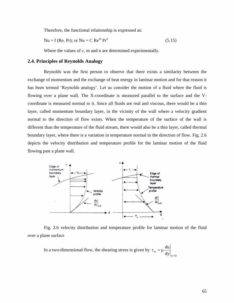
65

Therefore, the functional relationship is expressed as:

Nu = f (Re, Pr); or Nu = C Rem

Prn (5.15)

Where the values of c, m and n are determined experimentally.

2.4. Principles of Reynolds Analogy

Reynolds was the first person to observe that there exists a similarity between the

exchange of momentum and the exchange of heat energy in laminar motion and for that reason it

has been termed ‘Reynolds analogy’. Let us consider the motion of a fluid where the fluid is

flowing over a plane wall. The X-coordinate is measured parallel to the surface and the V-

coordinate is measured normal to it. Since all fluids are real and viscous, there would be a thin

layer, called momentum boundary layer, in the vicinity of the wall where a velocity gradient

normal to the direction of flow exists. When the temperature of the surface of the wall is

different than the temperature of the fluid stream, there would also be a thin layer, called thermal

boundary layer, where there is a variation in temperature normal to the direction of flow. Fig. 2.6

depicts the velocity distribution and temperature profile for the laminar motion of the fluid

flowing past a plane wall.

Fig. 2.6 velocity distribution and temperature profile for laminar motion of the fluid

over a plane surface

In a two-dimensional flow, the shearing stress is given by w

y 0

du

dy

66

and the rate of heat transfer per unit area is given by wkQ dT

A du

For Pr = Cp/k = 1, we have k/ = Cp and therefore, we can write after separating the

variables,

w p

Qdu dT

A C

(5.16)

Assuming that Q and w are constant at any station x, we integrate equation (5.16)

between the limits: u = 0 when T = Tw , and u = U when T = T , and we get,

w p wQ/ A C U T T

Since by definition, x wQ / A h T T , and 2

w fxC U / 2,

Where fxC , is the skin friction coefficient at the station x. We have

fxC /2 = hx/ (CpU ) (5.17)

Since x p x. p xh / C U h x / k / U k / .C Nu / Re.Pr ,

x fxNu / Re.Pr C / 2 Stan tonnumer,St. (5.18)

Equation (5.18) is satisfactory for gases in which Pr is approximately equal to unity.

Colburn has shown that Eq. (5.18) can also be used for fluids having Prandtl numbers ranging

from 0.6 to about 50 if it is modified in accordance with experirnental results.

Or, 2 / 3 2 / 3xx fx

x

Nu.Pr St Pr C / 2

Re Pr (5.19)

Eq. (5.19) expresses the relation between fluid friction and heat transfer for laminar

flow over a plane wall. The heat transfer coefficient could thus be determined by making

measurements of the frictional drag on a plate under conditions in which no heat transfer is

involved.

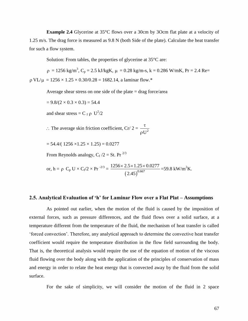
67

Example 2.4 Glycerine at 35°C flows over a 30cm by 3Ocm flat plate at a velocity of

1.25 m/s. The drag force is measured as 9.8 N (both Side of the plate). Calculate the heat transfer

for such a flow system.

Solution: From tables, the properties of glycerine at 35°C are:

= 1256 kg/m3, Cp = 2.5 kJ/kgK, = 0.28 kg/m-s, k = 0.286 W/mK, Pr = 2.4 Re=

VL/ = 1256 × 1.25 × 0.30/0.28 = 1682.14, a laminar flow.*

Average shear stress on one side of the plate = drag force/area

= 9.8/(2 × 0.3 × 0.3) = 54.4

and shear stress = C f U2/2

The average skin friction coefficient, Cr/ 2 = 2U

= 54.4/( 1256 ×1.25 × 1.25) = 0.0277

From Reynolds analogy, Cf /2 = St. Pr 2/3

or, h = Cp U × Cf/2 × Pr -2/3

=

0.667

1256 2.5 1.25 0.0277

2.45

=59.8 kW/m

2K.

2.5. Analytical Evaluation of ‘h’ for Laminar Flow over a Flat Plat – Assumptions

As pointed out earlier, when the motion of the fluid is caused by the imposition of

external forces, such as pressure differences, and the fluid flows over a solid surface, at a

temperature different from the temperature of the fluid, the mechanism of heat transfer is called

‘forced convection’. Therefore, any analytical approach to determine the convective heat transfer

coefficient would require the temperature distribution in the flow field surrounding the body.

That is, the theoretical analysis would require the use of the equation of motion of the viscous

fluid flowing over the body along with the application of the principles of conservation of mass

and energy in order to relate the heat energy that is convected away by the fluid from the solid

surface.

For the sake of simplicity, we will consider the motion of the fluid in 2 space

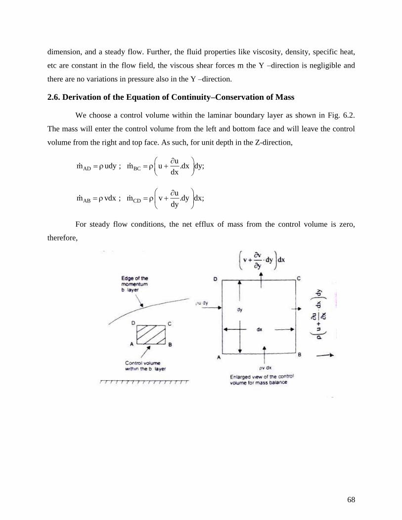
68

dimension, and a steady flow. Further, the fluid properties like viscosity, density, specific heat,

etc are constant in the flow field, the viscous shear forces m the Y –direction is negligible and

there are no variations in pressure also in the Y –direction.

2.6. Derivation of the Equation of Continuity–Conservation of Mass

We choose a control volume within the laminar boundary layer as shown in Fig. 6.2.

The mass will enter the control volume from the left and bottom face and will leave the control

volume from the right and top face. As such, for unit depth in the Z-direction,

AD BC

um udy ; m u .dx dy;

dx

AB CD

um vdx ; m v .dy dx;

dy

For steady flow conditions, the net efflux of mass from the control volume is zero,

therefore,

69

Fig. 2.7 a differential control volume within the boundary layer for laminar flow over a

plane wall

u vudy xdx udy dxdy vdx .dxdy

x x

or, u / x v y 0, the equation of continuity. (2.20)

Concept of Critical Thickness of Insulation

The addition of insulation at the outside surface of small pipes may not reduce the rate

of heat transfer. When an insulation is added on the outer surface of a bare pipe, its outer radius,

r0 increases and this increases the thermal resistance due to conduction logarithmically whereas t

he thermal resistance to heat flow due to fluid film on the outer surface decreases linearly with

increasing radius, r0. Since the total thermal resistance is proportional to the sum of these two

resistances, the rate of heat flow may not decrease as insulation is added to the bare pipe.

Fig. 2.7 shows a plot of heat loss against the insulation radius for two different cases.

For small pipes or wires, the radius rl may be less than re and in that case, addition of insulation

to the bare pipe will increase the heat loss until the critical radius is reached. Further addition of

insulation will decrease the heat loss rate from this peak value. The insulation thickness (r* – rl)

must be added to reduce the heat loss below the uninsulated rate. If the outer pipe radius rl is

greater than the critical radius re any insulation added will decrease the heat loss.

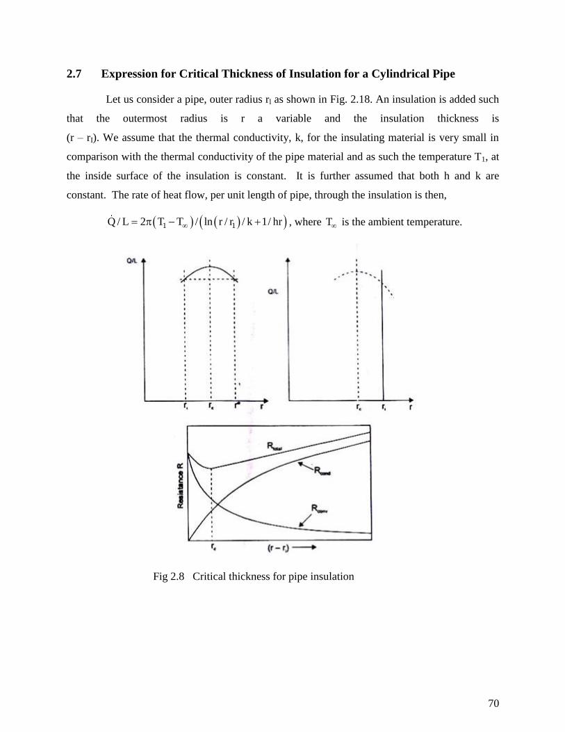
70

2.7 Expression for Critical Thickness of Insulation for a Cylindrical Pipe

Let us consider a pipe, outer radius rl as shown in Fig. 2.18. An insulation is added such

that the outermost radius is r a variable and the insulation thickness is

(r – rI). We assume that the thermal conductivity, k, for the insulating material is very small in

comparison with the thermal conductivity of the pipe material and as such the temperature T1, at

the inside surface of the insulation is constant. It is further assumed that both h and k are

constant. The rate of heat flow, per unit length of pipe, through the insulation is then,

1 1Q / L 2 T T / ln r / r / k 1/ hr , where T is the ambient temperature.

Fig 2.8 Critical thickness for pipe insulation

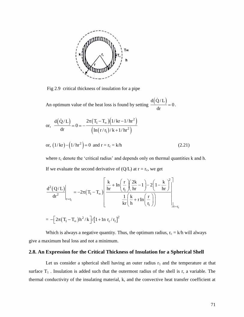
71

Fig 2.9 critical thickness of insulation for a pipe

An optimum value of the heat loss is found by setting d Q / L

0dr

.

or,

21

21

2 T T 1/ kr 1/ hrd Q / L0

dr ln r / r / k 1/ hr

or, 21/ kr 1/ hr 0 and r = rc = k/h (2.21)

where rc denote the ‘critical radius’ and depends only on thermal quantities k and h.

If we evaluate the second derivative of (Q/L) at r = rc, we get

c

c

2

21

12

r r

1 r r

k r 2k kIn 1 2 1

d Q/ L hr r hr hr2 T T

dr 1 k rr In

kr h r

= 22

1 c 12 T T h / k / 1 1n r / r

Which is always a negative quantity. Thus, the optimum radius, rc = k/h will always

give a maximum heal loss and not a minimum.

2.8. An Expression for the Critical Thickness of Insulation for a Spherical Shell

Let us consider a spherical shell having an outer radius r1 and the temperature at that

surface T1 . Insulation is added such that the outermost radius of the shell is r, a variable. The

thermal conductivity of the insulating material, k, and the convective heat transfer coefficient at

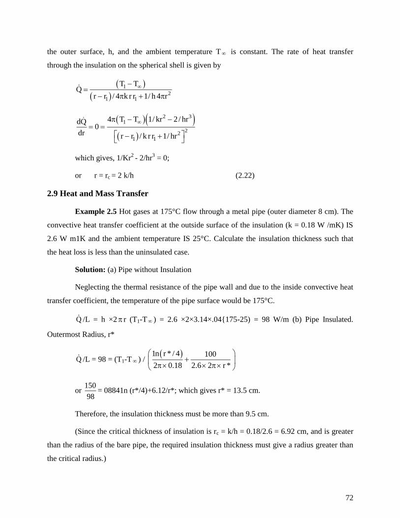
72

the outer surface, h, and the ambient temperature T is constant. The rate of heat transfer

through the insulation on the spherical shell is given by

1

21 1

T TQ

r r / 4 k r r 1/ h 4 r

2 31

22

1 1

4 T T 1/ kr 2/ hrdQ0

dr r r / k r r 1/ hr

which gives, 1/Kr2

- 2/hr3 = 0;

or r = rc = 2 k/h (2.22)

2.9 Heat and Mass Transfer

Example 2.5 Hot gases at 175°C flow through a metal pipe (outer diameter 8 cm). The

convective heat transfer coefficient at the outside surface of the insulation (k = 0.18 W /mK) IS

2.6 W m1K and the ambient temperature IS 25°C. Calculate the insulation thickness such that

the heat loss is less than the uninsulated case.

Solution: (a) Pipe without Insulation

Neglecting the thermal resistance of the pipe wall and due to the inside convective heat

transfer coefficient, the temperature of the pipe surface would be 175°C.

Q /L = h ×2 r (T1-T ) = 2.6 ×2×3.14×.04{175-25) = 98 W/m (b) Pipe Insulated.

Outermost Radius, r*

Q /L = 98 = (T1-T ) / 1n r * / 4 100

2 0.18 2.6 2 r *

or 150

98= 08841n (r*/4)+6.12/r*; which gives r* = 13.5 cm.

Therefore, the insulation thickness must be more than 9.5 cm.

(Since the critical thickness of insulation is rc = k/h = 0.18/2.6 = 6.92 cm, and is greater

than the radius of the bare pipe, the required insulation thickness must give a radius greater than

the critical radius.)

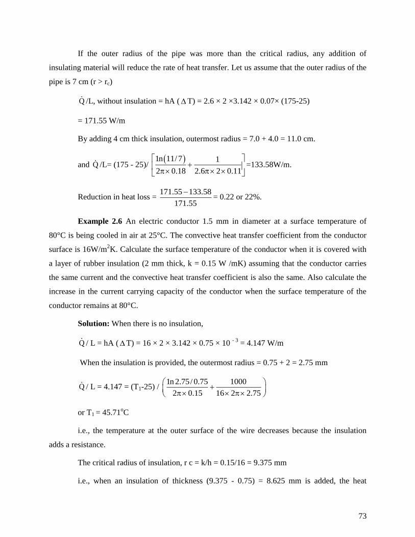
73

If the outer radius of the pipe was more than the critical radius, any addition of

insulating material will reduce the rate of heat transfer. Let us assume that the outer radius of the

pipe is 7 cm (r > rc)

Q /L, without insulation = hA (T) = 2.6 × 2 ×3.142 × 0.07× (175-25)

= 171.55 W/m

By adding 4 cm thick insulation, outermost radius = 7.0 + 4.0 = 11.0 cm.

and Q /L= (175 - 25)/ 1n 11/ 7 1

2 0.18 2.6 2 0.11

=133.58W/m.

Reduction in heat loss = 171.55 133.58

171.55

= 0.22 or 22%.

Example 2.6 An electric conductor 1.5 mm in diameter at a surface temperature of

80°C is being cooled in air at 25°C. The convective heat transfer coefficient from the conductor

surface is 16W/m2K. Calculate the surface temperature of the conductor when it is covered with

a layer of rubber insulation (2 mm thick, k = 0.15 W /mK) assuming that the conductor carries

the same current and the convective heat transfer coefficient is also the same. Also calculate the

increase in the current carrying capacity of the conductor when the surface temperature of the

conductor remains at 80°C.

Solution: When there is no insulation,

Q / L = hA (T) = 16 × 2 × 3.142 × 0.75 × 10 - 3

= 4.147 W/m

When the insulation is provided, the outermost radius = 0.75 + 2 = 2.75 mm

Q / L = 4.147 = (T1-25) / 1n 2.75/ 0.75 1000

2 0.15 16 2 2.75

or T1 = 45.71oC

i.e., the temperature at the outer surface of the wire decreases because the insulation

adds a resistance.

The critical radius of insulation, r c = k/h = 0.15/16 = 9.375 mm

i.e., when an insulation of thickness (9.375 - 0.75) = 8.625 mm is added, the heat

74

transfer rate would be the maximum and the conductor can carry more current. The heat transfer

rate with outermost radius equal to rc = 9.375 mm

Q /L = (80 - 25) / 1n9.375/ 0.75 1000

2 0.15 16 2 9.375

=14.7 W/m

The rate of heat transfer is proportional to (current)2, the new current I2 would be:

I2/I1 = (14.7 / 4.147)1/2

= 1.883

or, the current carrying capacity can be increased 1.883 times. But the maximum current

capacity of wire would be limited by the permissible temperature at the centre of the wire.

The surface temperature of the conductor when the outermost radius with insulation is

equal to the critical radius, is given by

Q /L = 4.147 = (T-25/ 1n9.375/ 0.75 1000

2 3.142 0.15 16 2 3.142 9.375

or T = 40.83°C.

75

SCHOOL OF MECHANICAL

DEPARTMENT OF MECHANICAL

UNIT – III – Heat and mass transfer – SMEA1504

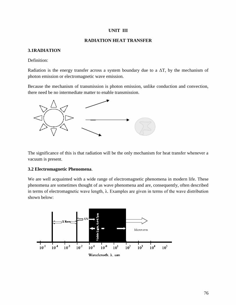
76

UNIT III

RADIATION HEAT TRANSFER

3.1RADIATION

Definition:

Radiation is the energy transfer across a system boundary due to a ΔT, by the mechanism of

photon emission or electromagnetic wave emission.

Because the mechanism of transmission is photon emission, unlike conduction and convection,

there need be no intermediate matter to enable transmission.

The significance of this is that radiation will be the only mechanism for heat transfer whenever a

vacuum is present.

3.2 Electromagnetic Phenomena.

We are well acquainted with a wide range of electromagnetic phenomena in modern life. These

phenomena are sometimes thought of as wave phenomena and are, consequently, often described

in terms of electromagnetic wave length, λ. Examples are given in terms of the wave distribution

shown below:

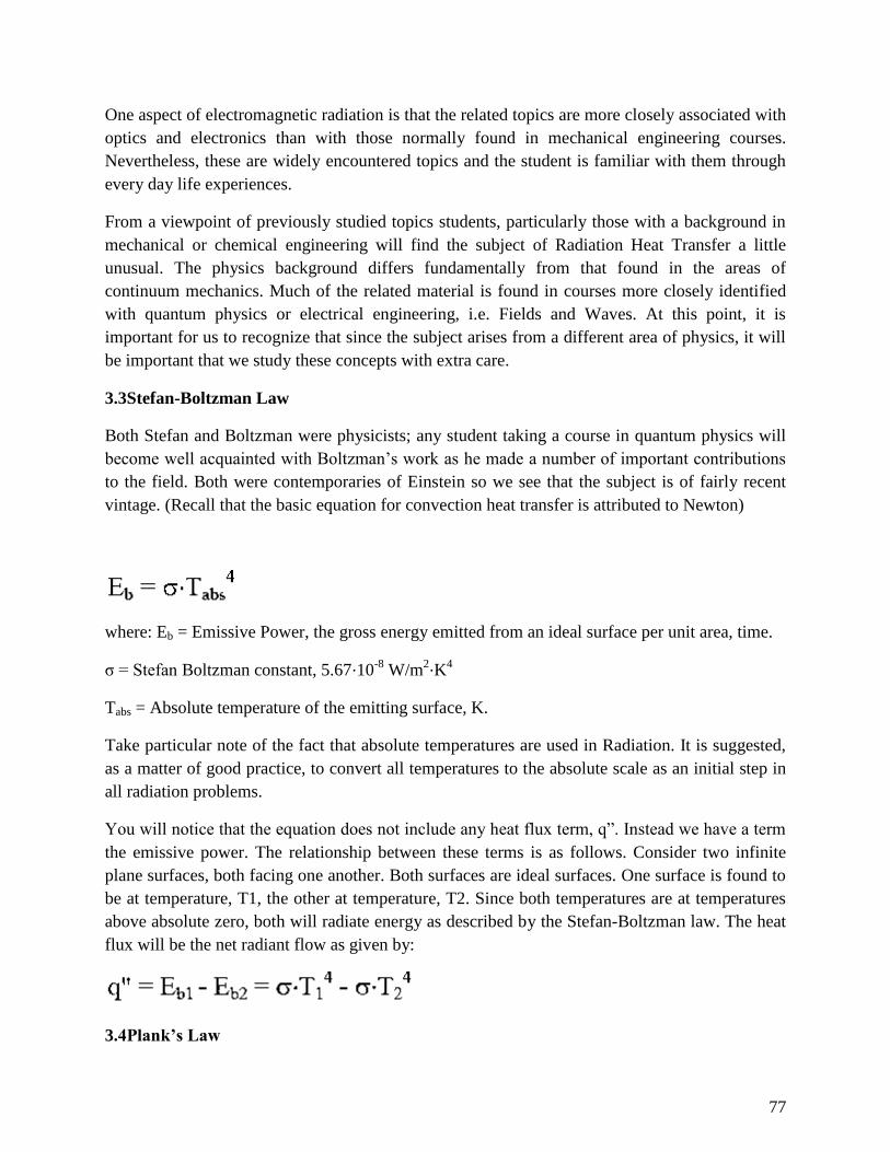
77

One aspect of electromagnetic radiation is that the related topics are more closely associated with

optics and electronics than with those normally found in mechanical engineering courses.

Nevertheless, these are widely encountered topics and the student is familiar with them through

every day life experiences.

From a viewpoint of previously studied topics students, particularly those with a background in

mechanical or chemical engineering will find the subject of Radiation Heat Transfer a little

unusual. The physics background differs fundamentally from that found in the areas of

continuum mechanics. Much of the related material is found in courses more closely identified

with quantum physics or electrical engineering, i.e. Fields and Waves. At this point, it is

important for us to recognize that since the subject arises from a different area of physics, it will

be important that we study these concepts with extra care.

3.3Stefan-Boltzman Law

Both Stefan and Boltzman were physicists; any student taking a course in quantum physics will

become well acquainted with Boltzman’s work as he made a number of important contributions

to the field. Both were contemporaries of Einstein so we see that the subject is of fairly recent

vintage. (Recall that the basic equation for convection heat transfer is attributed to Newton)

where: Eb = Emissive Power, the gross energy emitted from an ideal surface per unit area, time.

σ = Stefan Boltzman constant, 5.67⋅10-8

W/m2⋅K4

Tabs = Absolute temperature of the emitting surface, K.

Take particular note of the fact that absolute temperatures are used in Radiation. It is suggested,

as a matter of good practice, to convert all temperatures to the absolute scale as an initial step in

all radiation problems.

You will notice that the equation does not include any heat flux term, q”. Instead we have a term

the emissive power. The relationship between these terms is as follows. Consider two infinite

plane surfaces, both facing one another. Both surfaces are ideal surfaces. One surface is found to

be at temperature, T1, the other at temperature, T2. Since both temperatures are at temperatures

above absolute zero, both will radiate energy as described by the Stefan-Boltzman law. The heat

flux will be the net radiant flow as given by:

3.4Plank’s Law

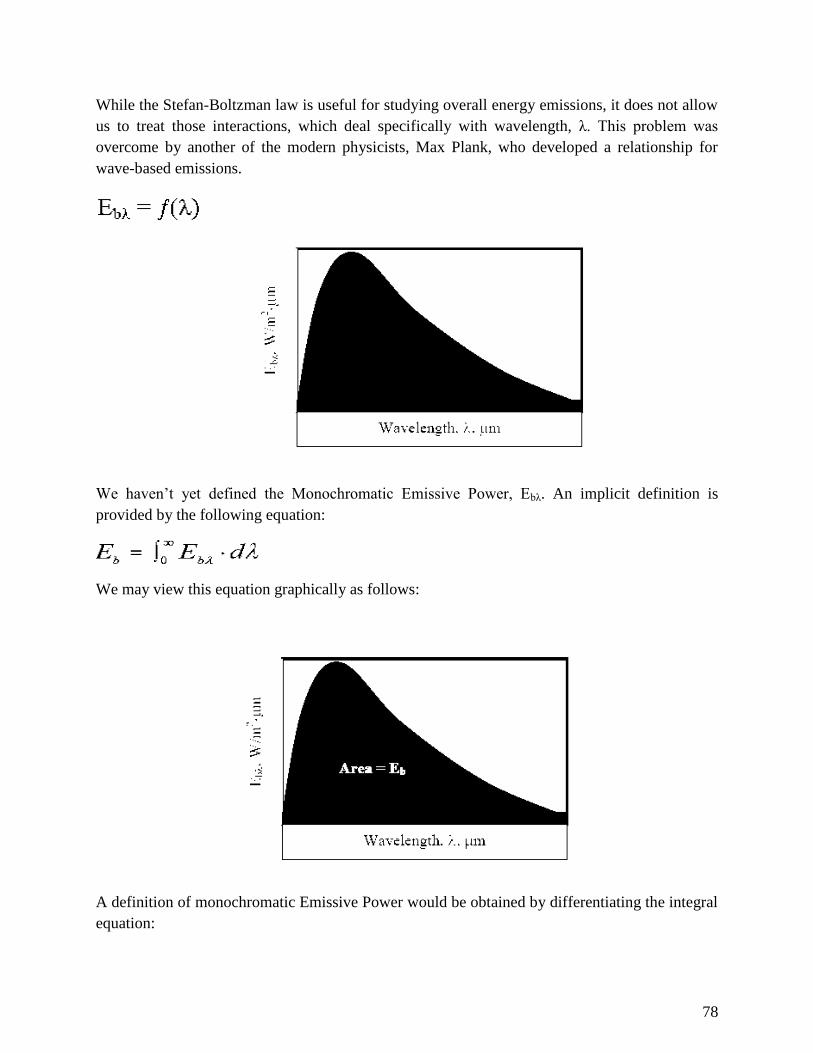
78

While the Stefan-Boltzman law is useful for studying overall energy emissions, it does not allow

us to treat those interactions, which deal specifically with wavelength, λ. This problem was

overcome by another of the modern physicists, Max Plank, who developed a relationship for

wave-based emissions.

We haven’t yet defined the Monochromatic Emissive Power, Ebλ. An implicit definition is

provided by the following equation:

We may view this equation graphically as follows:

A definition of monochromatic Emissive Power would be obtained by differentiating the integral

equation:

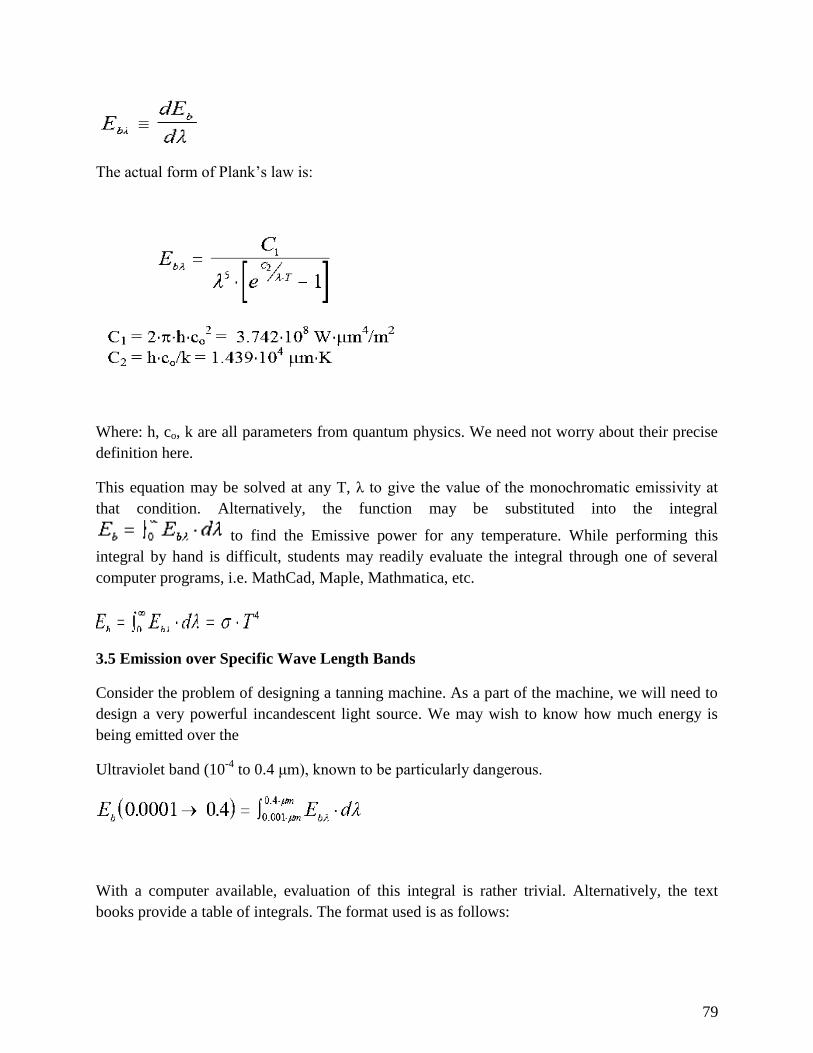
79

The actual form of Plank’s law is:

Where: h, co, k are all parameters from quantum physics. We need not worry about their precise

definition here.

This equation may be solved at any T, λ to give the value of the monochromatic emissivity at

that condition. Alternatively, the function may be substituted into the integral

to find the Emissive power for any temperature. While performing this

integral by hand is difficult, students may readily evaluate the integral through one of several

computer programs, i.e. MathCad, Maple, Mathmatica, etc.

3.5 Emission over Specific Wave Length Bands

Consider the problem of designing a tanning machine. As a part of the machine, we will need to

design a very powerful incandescent light source. We may wish to know how much energy is

being emitted over the

Ultraviolet band (10-4

to 0.4 μm), known to be particularly dangerous.

With a computer available, evaluation of this integral is rather trivial. Alternatively, the text

books provide a table of integrals. The format used is as follows:

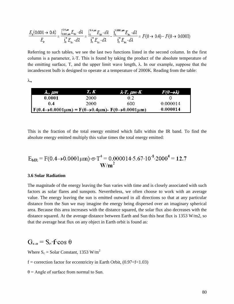
80

Referring to such tables, we see the last two functions listed in the second column. In the first

column is a parameter, λ⋅T. This is found by taking the product of the absolute temperature of

the emitting surface, T, and the upper limit wave length, λ. In our example, suppose that the

incandescent bulb is designed to operate at a temperature of 2000K. Reading from the table:

λ.,

This is the fraction of the total energy emitted which falls within the IR band. To find the

absolute energy emitted multiply this value times the total energy emitted:

3.6 Solar Radiation

The magnitude of the energy leaving the Sun varies with time and is closely associated with such

factors as solar flares and sunspots. Nevertheless, we often choose to work with an average

value. The energy leaving the sun is emitted outward in all directions so that at any particular

distance from the Sun we may imagine the energy being dispersed over an imaginary spherical

area. Because this area increases with the distance squared, the solar flux also decreases with the

distance squared. At the average distance between Earth and Sun this heat flux is 1353 W/m2, so

that the average heat flux on any object in Earth orbit is found as:

Where Sc = Solar Constant, 1353 W/m2

f = correction factor for eccentricity in Earth Orbit, (0.97<f<1.03)

θ = Angle of surface from normal to Sun.

81

Because of reflection and absorption in the Earth’s atmosphere, this number is significantly

reduced at ground level. Nevertheless, this value gives us some opportunity to estimate the

potential for using solar energy, such as in photovoltaic cells.

Some Definitions

In the previous section we introduced the Stefan-Boltzman Equation to describe radiation from

an ideal surface.

This equation provides a method of determining the total energy leaving a surface, but gives no

indication of the direction in which it travels. As we continue our study, we will want to be able

to calculate how heat is distributed among various objects.

For this purpose, we will introduce the radiation intensity, I, defined as the energy emitted per

unit area, per unit time, per unit solid angle. Before writing an equation for this new property, we

will need to define some of the terms we will be using.

3.7 Angles and Arc Length

We are well accustomed to thinking of an angle as a two dimensional object. It may be used to

find an arc length:

Solid Angle

We generalize the idea of an angle and an arc length to three dimensions and define a solid

angle, Ω, which like the standard angle has no dimensions. The solid angle, when multiplied by

the radius squared will have dimensions of length squared, or area, and will have the magnitude

of the encompassed area.

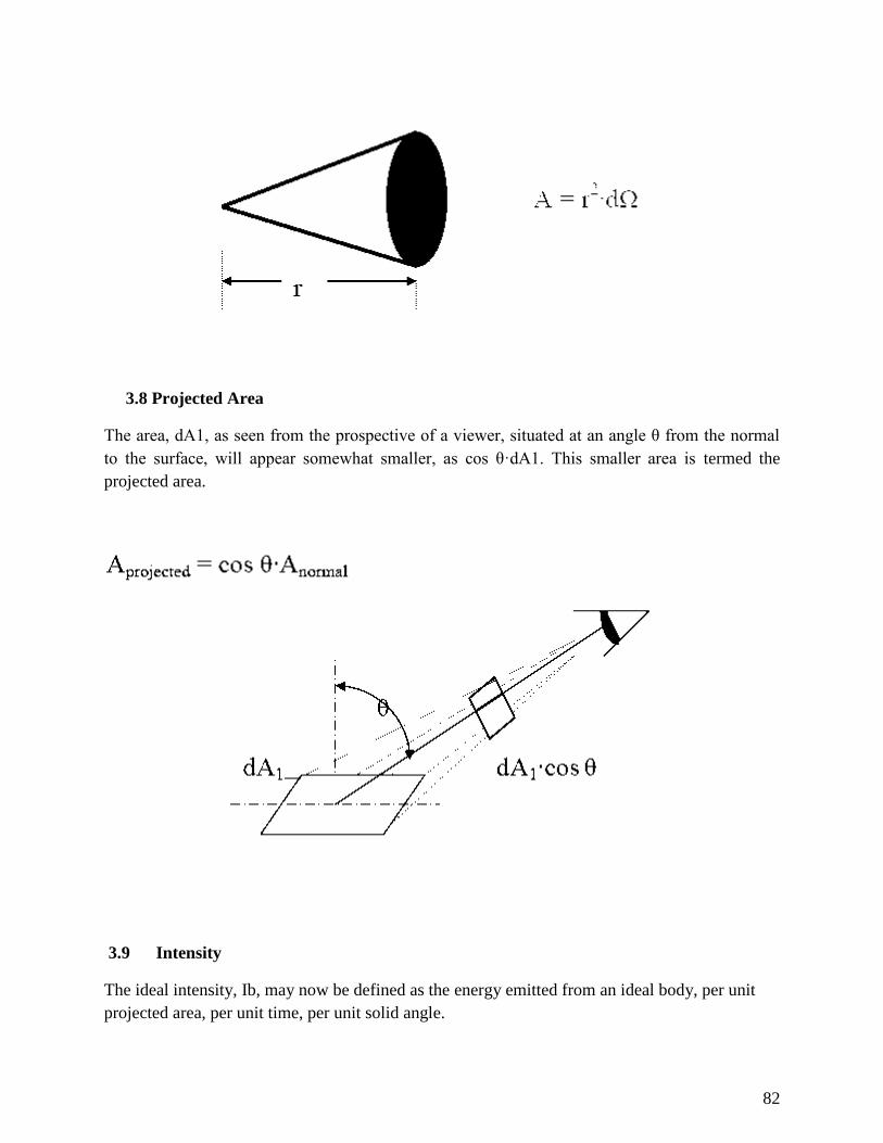
82

3.8 Projected Area

The area, dA1, as seen from the prospective of a viewer, situated at an angle θ from the normal

to the surface, will appear somewhat smaller, as cos θ·dA1. This smaller area is termed the

projected area.

3.9 Intensity

The ideal intensity, Ib, may now be defined as the energy emitted from an ideal body, per unit

projected area, per unit time, per unit solid angle.

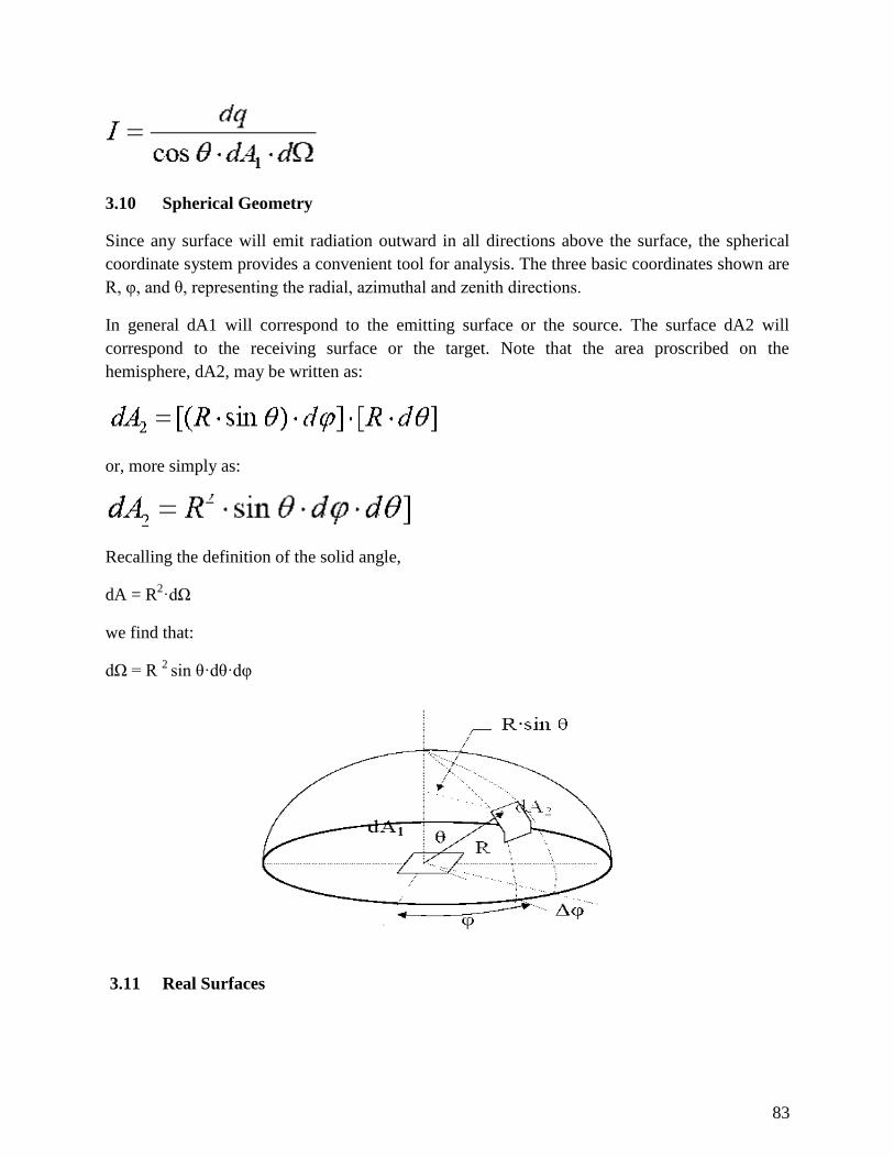
83

3.10 Spherical Geometry

Since any surface will emit radiation outward in all directions above the surface, the spherical

coordinate system provides a convenient tool for analysis. The three basic coordinates shown are

R, φ, and θ, representing the radial, azimuthal and zenith directions.

In general dA1 will correspond to the emitting surface or the source. The surface dA2 will

correspond to the receiving surface or the target. Note that the area proscribed on the

hemisphere, dA2, may be written as:

or, more simply as:

Recalling the definition of the solid angle,

dA = R2·dΩ

we find that:

dΩ = R 2

sin θ·dθ·dφ

3.11 Real Surfaces

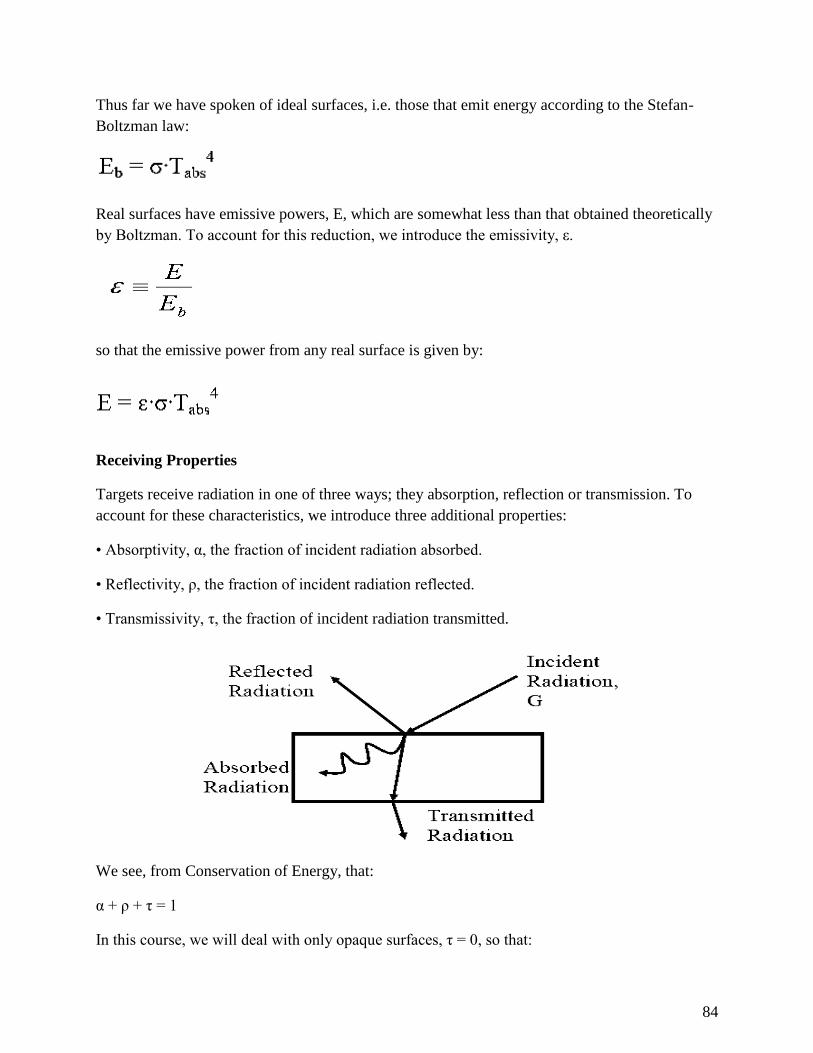
84

Thus far we have spoken of ideal surfaces, i.e. those that emit energy according to the Stefan-

Boltzman law:

Real surfaces have emissive powers, E, which are somewhat less than that obtained theoretically

by Boltzman. To account for this reduction, we introduce the emissivity, ε.

so that the emissive power from any real surface is given by:

Receiving Properties

Targets receive radiation in one of three ways; they absorption, reflection or transmission. To

account for these characteristics, we introduce three additional properties:

• Absorptivity, α, the fraction of incident radiation absorbed.

• Reflectivity, ρ, the fraction of incident radiation reflected.

• Transmissivity, τ, the fraction of incident radiation transmitted.

We see, from Conservation of Energy, that:

α + ρ + τ = 1

In this course, we will deal with only opaque surfaces, τ = 0, so that:

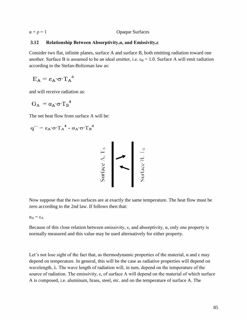
85

α + ρ = 1 Opaque Surfaces

3.12 Relationship Between Absorptivity,α, and Emissivity,ε

Consider two flat, infinite planes, surface A and surface B, both emitting radiation toward one

another. Surface B is assumed to be an ideal emitter, i.e. εB = 1.0. Surface A will emit radiation

according to the Stefan-Boltzman law as:

and will receive radiation as:

The net heat flow from surface A will be:

Now suppose that the two surfaces are at exactly the same temperature. The heat flow must be

zero according to the 2nd law. If follows then that:

αA = εA

Because of this close relation between emissivity, ε, and absorptivity, α, only one property is

normally measured and this value may be used alternatively for either property.

Let’s not lose sight of the fact that, as thermodynamic properties of the material, α and ε may

depend on temperature. In general, this will be the case as radiative properties will depend on

wavelength, λ. The wave length of radiation will, in turn, depend on the temperature of the

source of radiation. The emissivity, ε, of surface A will depend on the material of which surface

A is composed, i.e. aluminum, brass, steel, etc. and on the temperature of surface A. The

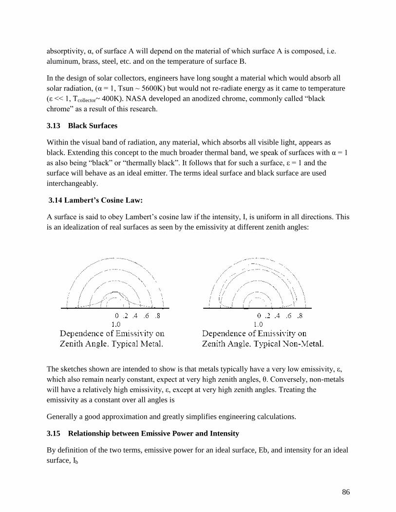
86

absorptivity, α, of surface A will depend on the material of which surface A is composed, i.e.

aluminum, brass, steel, etc. and on the temperature of surface B.

In the design of solar collectors, engineers have long sought a material which would absorb all

solar radiation, (α = 1, Tsun ~ 5600K) but would not re-radiate energy as it came to temperature

(ε << 1, Tcollector~ 400K). NASA developed an anodized chrome, commonly called “black

chrome” as a result of this research.

3.13 Black Surfaces

Within the visual band of radiation, any material, which absorbs all visible light, appears as

black. Extending this concept to the much broader thermal band, we speak of surfaces with α = 1

as also being “black” or “thermally black”. It follows that for such a surface, ε = 1 and the

surface will behave as an ideal emitter. The terms ideal surface and black surface are used

interchangeably.

3.14 Lambert’s Cosine Law:

A surface is said to obey Lambert’s cosine law if the intensity, I, is uniform in all directions. This

is an idealization of real surfaces as seen by the emissivity at different zenith angles:

The sketches shown are intended to show is that metals typically have a very low emissivity, ε,

which also remain nearly constant, expect at very high zenith angles, θ. Conversely, non-metals

will have a relatively high emissivity, ε, except at very high zenith angles. Treating the

emissivity as a constant over all angles is

Generally a good approximation and greatly simplifies engineering calculations.

3.15 Relationship between Emissive Power and Intensity

By definition of the two terms, emissive power for an ideal surface, Eb, and intensity for an ideal

surface, Ib

87

Replacing the solid angle by its equivalent in spherical angles:

Integrate once, holding Ib constant:

Integrate a second time. (Note that the derivative of sin θ is cos θ·dθ.)

3.16 Radiation Exchange

During the previous lecture we introduced the intensity, I, to describe radiation within a

particular solid angle.

This will now be used to determine the fraction of radiation leaving a given surface and striking

a second surface.

Rearranging the above equation to express the heat radiated:

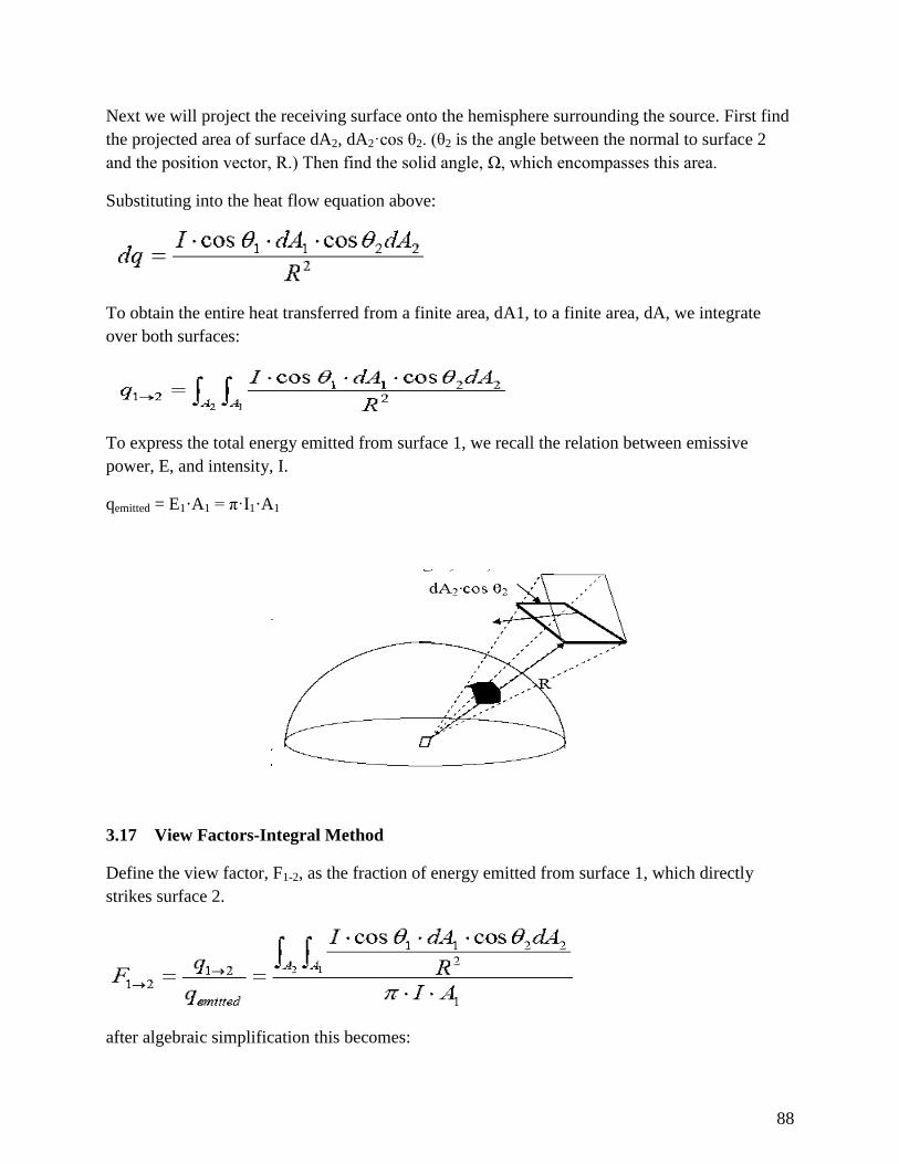
88

Next we will project the receiving surface onto the hemisphere surrounding the source. First find

the projected area of surface dA2, dA2·cos θ2. (θ2 is the angle between the normal to surface 2

and the position vector, R.) Then find the solid angle, Ω, which encompasses this area.

Substituting into the heat flow equation above:

To obtain the entire heat transferred from a finite area, dA1, to a finite area, dA, we integrate

over both surfaces:

To express the total energy emitted from surface 1, we recall the relation between emissive

power, E, and intensity, I.

qemitted = E1·A1 = π·I1·A1

3.17 View Factors-Integral Method

Define the view factor, F1-2, as the fraction of energy emitted from surface 1, which directly

strikes surface 2.

after algebraic simplification this becomes:

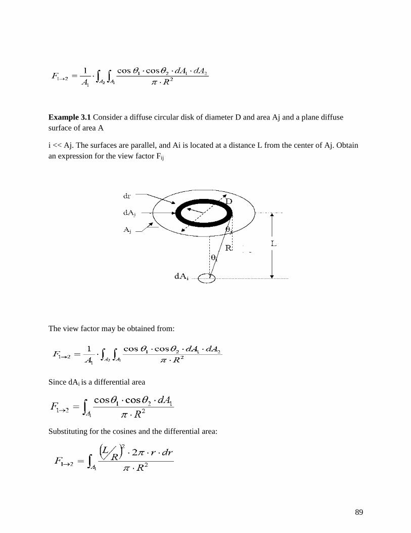
89

Example 3.1 Consider a diffuse circular disk of diameter D and area Aj and a plane diffuse

surface of area A

i << Aj. The surfaces are parallel, and Ai is located at a distance L from the center of Aj. Obtain

an expression for the view factor Fij

The view factor may be obtained from:

Since dAi is a differential area

Substituting for the cosines and the differential area:

90

After simplifying:

After integrating,

Substituting the upper & lower limits

This is but one example of how the view factor may be evaluated using the integral method. The

approach used here is conceptually quite straight forward; evaluating the integrals and

algebraically simplifying the resulting equations can be quite lengthy.

Enclosures

In order that we might apply conservation of energy to the radiation process, we must account

for all energy leaving a surface. We imagine that the surrounding surfaces act as an enclosure

about the heat source which receives all emitted energy. Should there be an opening in this

enclosure through which energy might be lost, we place an imaginary surface across this opening

to intercept this portion of the emitted energy. For an N surfaced enclosure, we can then see that:

This relationship is known as “Conservation Rule”.

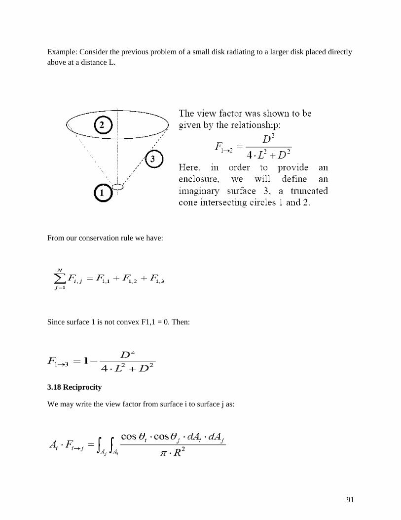
91

Example: Consider the previous problem of a small disk radiating to a larger disk placed directly

above at a distance L.

From our conservation rule we have:

Since surface 1 is not convex F1,1 = 0. Then:

3.18 Reciprocity

We may write the view factor from surface i to surface j as:

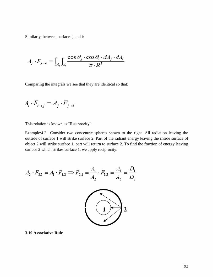
92

Similarly, between surfaces j and i:

Comparing the integrals we see that they are identical so that:

This relation is known as “Reciprocity”.

Example:4.2 Consider two concentric spheres shown to the right. All radiation leaving the

outside of surface 1 will strike surface 2. Part of the radiant energy leaving the inside surface of

object 2 will strike surface 1, part will return to surface 2. To find the fraction of energy leaving

surface 2 which strikes surface 1, we apply reciprocity:

3.19 Associative Rule

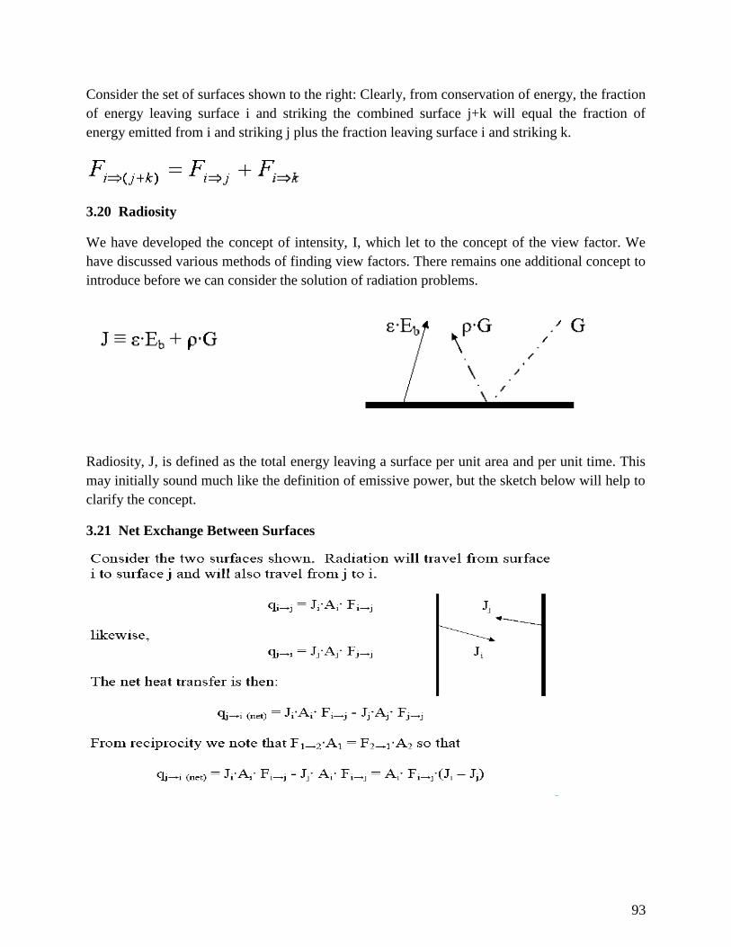
93

Consider the set of surfaces shown to the right: Clearly, from conservation of energy, the fraction

of energy leaving surface i and striking the combined surface j+k will equal the fraction of

energy emitted from i and striking j plus the fraction leaving surface i and striking k.

3.20 Radiosity

We have developed the concept of intensity, I, which let to the concept of the view factor. We

have discussed various methods of finding view factors. There remains one additional concept to

introduce before we can consider the solution of radiation problems.

Radiosity, J, is defined as the total energy leaving a surface per unit area and per unit time. This

may initially sound much like the definition of emissive power, but the sketch below will help to

clarify the concept.

3.21 Net Exchange Between Surfaces

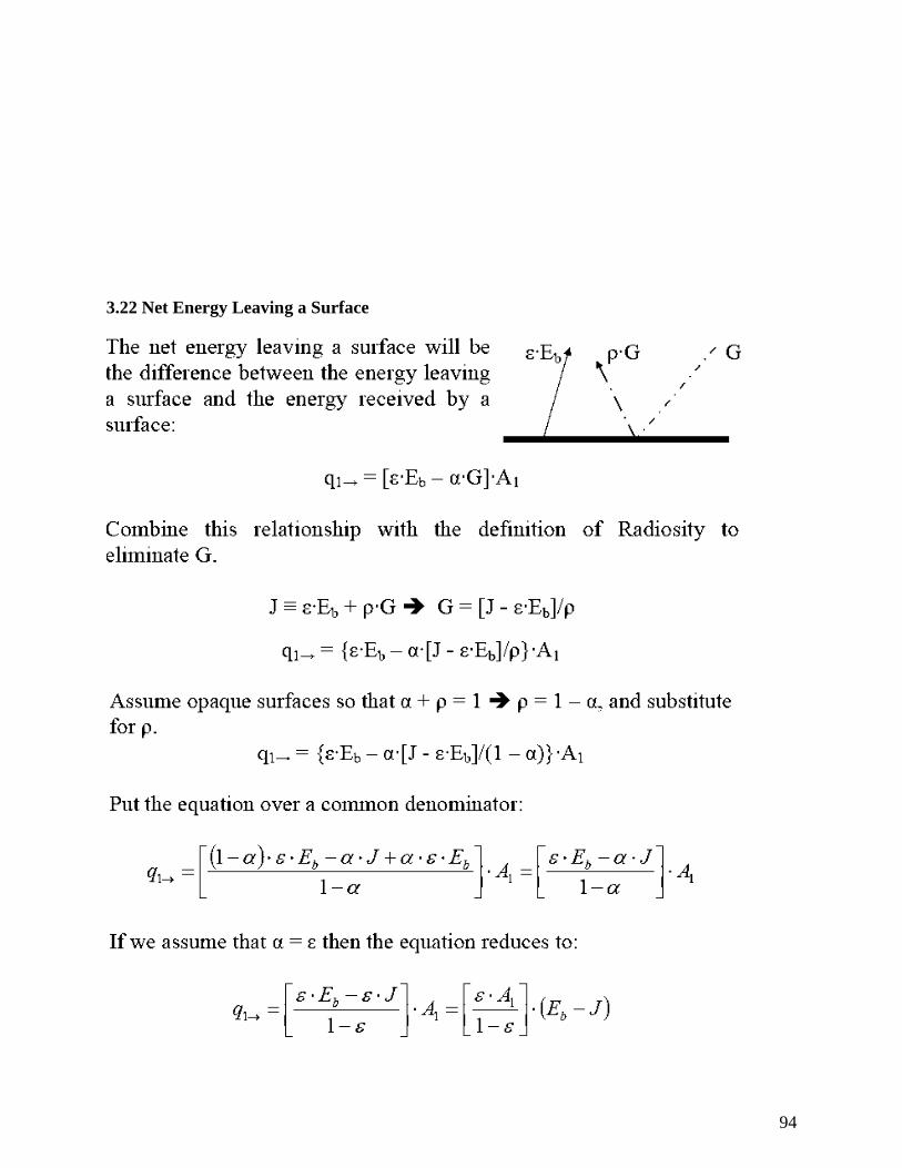
94

3.22 Net Energy Leaving a Surface

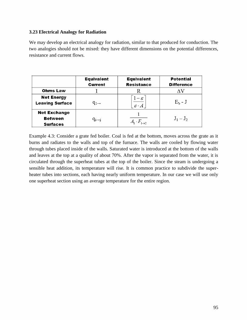
95

3.23 Electrical Analogy for Radiation

We may develop an electrical analogy for radiation, similar to that produced for conduction. The

two analogies should not be mixed: they have different dimensions on the potential differences,

resistance and current flows.

Example 4.3: Consider a grate fed boiler. Coal is fed at the bottom, moves across the grate as it

burns and radiates to the walls and top of the furnace. The walls are cooled by flowing water

through tubes placed inside of the walls. Saturated water is introduced at the bottom of the walls

and leaves at the top at a quality of about 70%. After the vapor is separated from the water, it is

circulated through the superheat tubes at the top of the boiler. Since the steam is undergoing a

sensible heat addition, its temperature will rise. It is common practice to subdivide the super-

heater tubes into sections, each having nearly uniform temperature. In our case we will use only

one superheat section using an average temperature for the entire region.

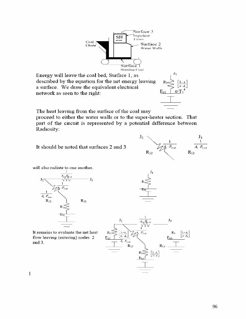
96

I

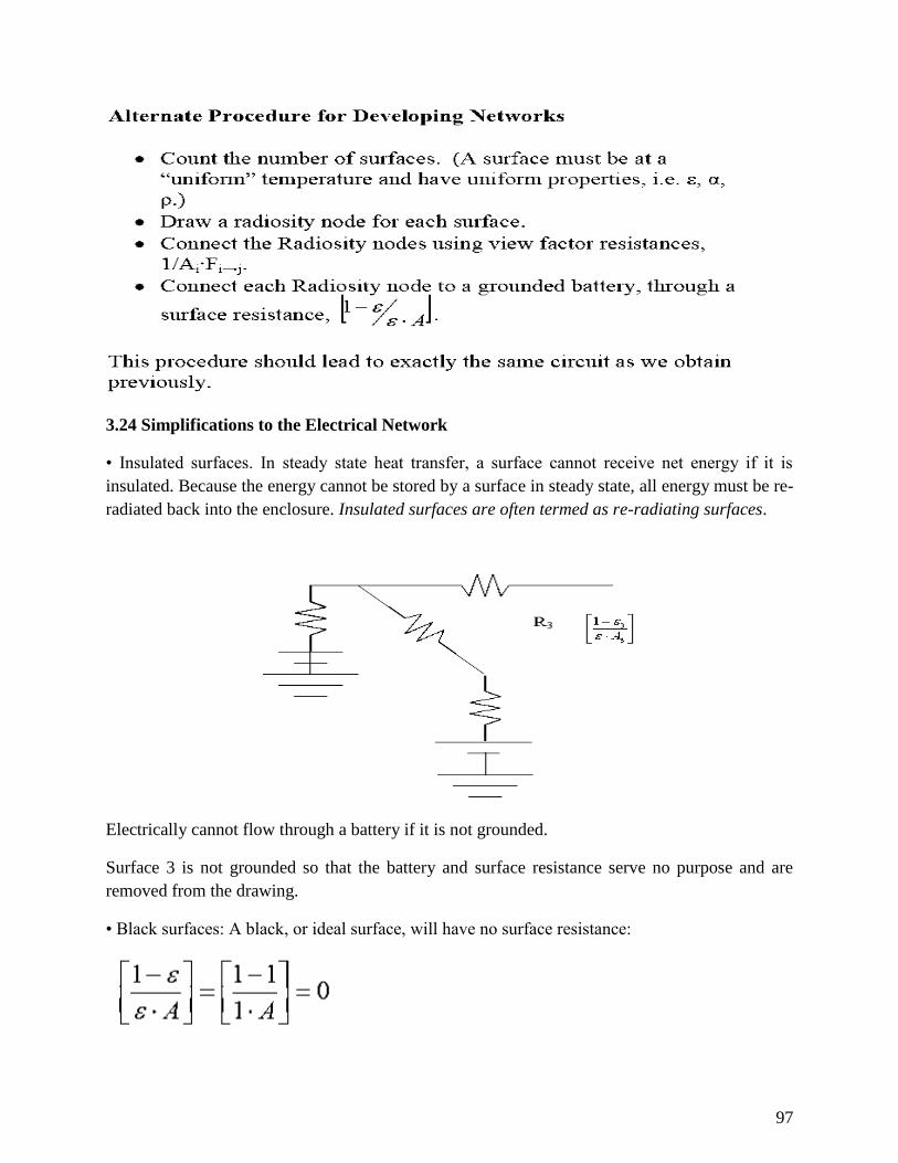
97

3.24 Simplifications to the Electrical Network

• Insulated surfaces. In steady state heat transfer, a surface cannot receive net energy if it is

insulated. Because the energy cannot be stored by a surface in steady state, all energy must be re-

radiated back into the enclosure. Insulated surfaces are often termed as re-radiating surfaces.

Electrically cannot flow through a battery if it is not grounded.

Surface 3 is not grounded so that the battery and surface resistance serve no purpose and are

removed from the drawing.

• Black surfaces: A black, or ideal surface, will have no surface resistance:

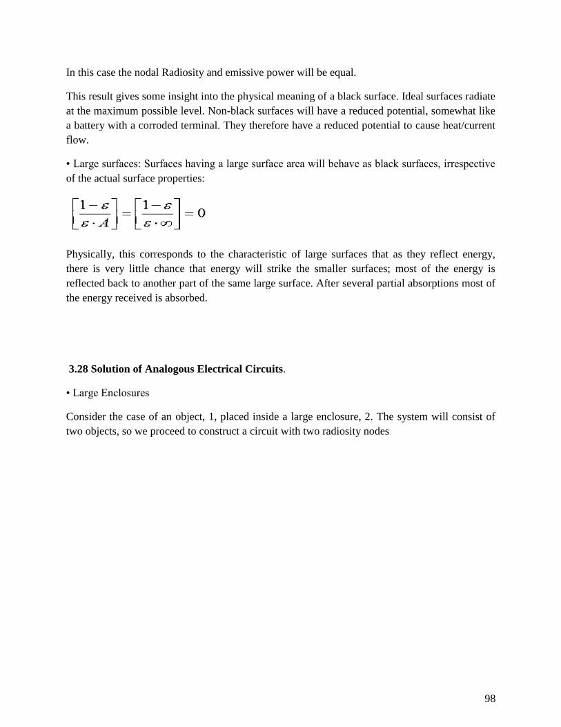
98

In this case the nodal Radiosity and emissive power will be equal.

This result gives some insight into the physical meaning of a black surface. Ideal surfaces radiate

at the maximum possible level. Non-black surfaces will have a reduced potential, somewhat like

a battery with a corroded terminal. They therefore have a reduced potential to cause heat/current

flow.

• Large surfaces: Surfaces having a large surface area will behave as black surfaces, irrespective

of the actual surface properties:

Physically, this corresponds to the characteristic of large surfaces that as they reflect energy,

there is very little chance that energy will strike the smaller surfaces; most of the energy is

reflected back to another part of the same large surface. After several partial absorptions most of

the energy received is absorbed.

3.28 Solution of Analogous Electrical Circuits.

• Large Enclosures

Consider the case of an object, 1, placed inside a large enclosure, 2. The system will consist of

two objects, so we proceed to construct a circuit with two radiosity nodes

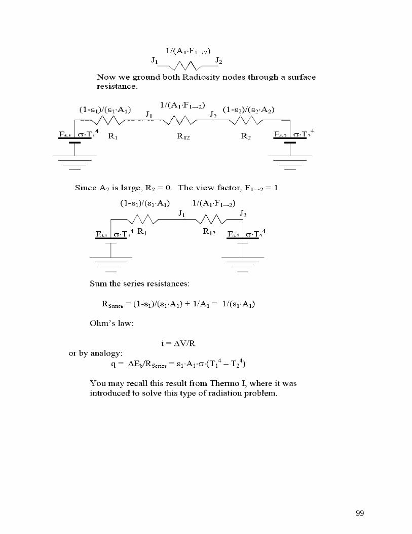
99

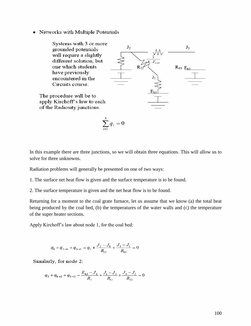
100

In this example there are three junctions, so we will obtain three equations. This will allow us to

solve for three unknowns.

Radiation problems will generally be presented on one of two ways:

1. The surface net heat flow is given and the surface temperature is to be found.

2. The surface temperature is given and the net heat flow is to be found.

Returning for a moment to the coal grate furnace, let us assume that we know (a) the total heat

being produced by the coal bed, (b) the temperatures of the water walls and (c) the temperature

of the super heater sections.

Apply Kirchoff’s law about node 1, for the coal bed:

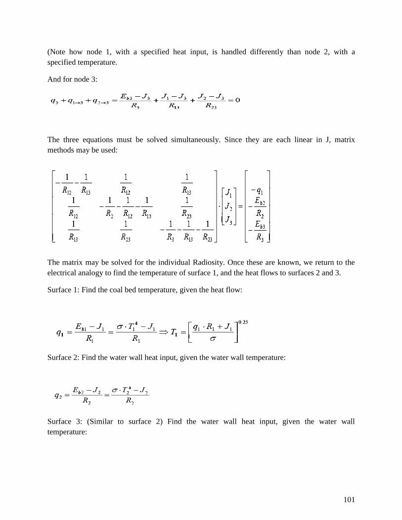
101

(Note how node 1, with a specified heat input, is handled differently than node 2, with a

specified temperature.

And for node 3:

The three equations must be solved simultaneously. Since they are each linear in J, matrix

methods may be used:

The matrix may be solved for the individual Radiosity. Once these are known, we return to the

electrical analogy to find the temperature of surface 1, and the heat flows to surfaces 2 and 3.

Surface 1: Find the coal bed temperature, given the heat flow:

Surface 2: Find the water wall heat input, given the water wall temperature:

Surface 3: (Similar to surface 2) Find the water wall heat input, given the water wall

temperature:

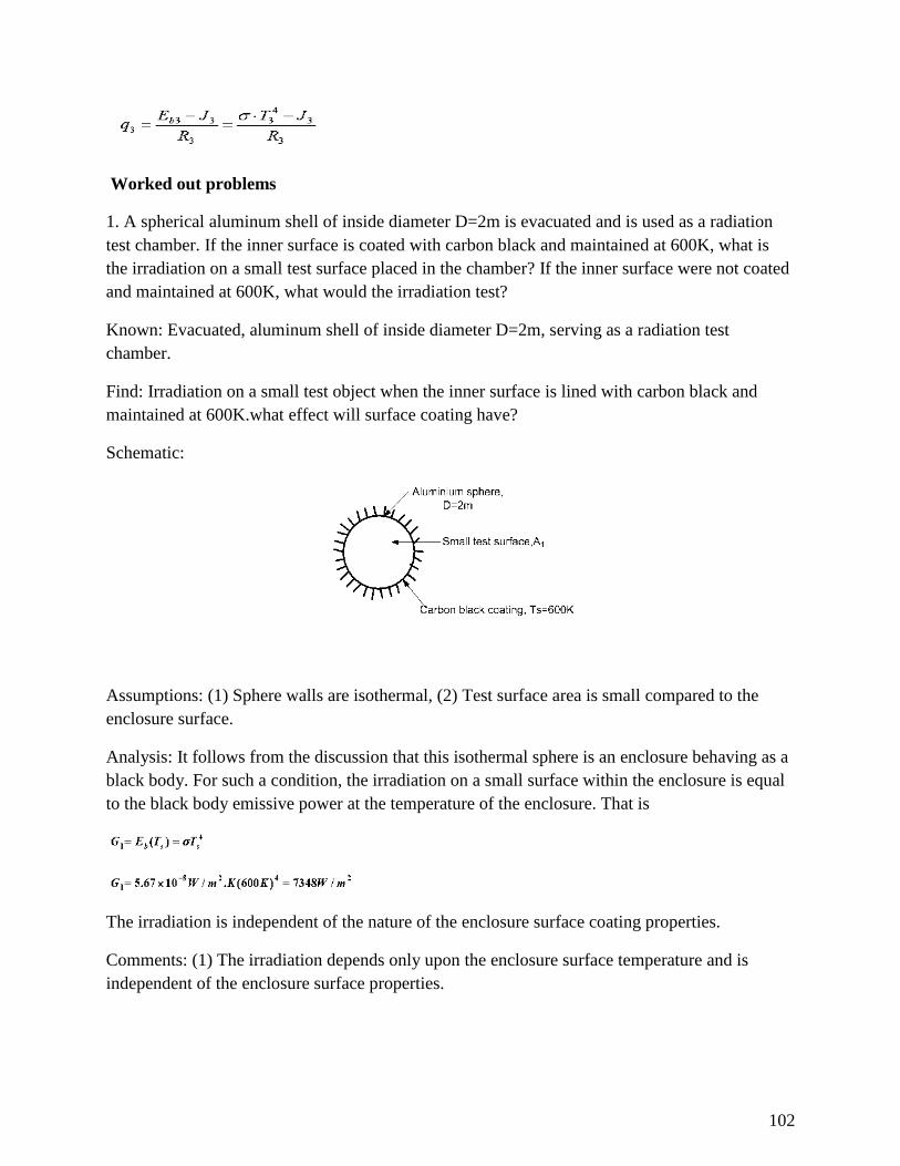
102

Worked out problems

1. A spherical aluminum shell of inside diameter D=2m is evacuated and is used as a radiation

test chamber. If the inner surface is coated with carbon black and maintained at 600K, what is

the irradiation on a small test surface placed in the chamber? If the inner surface were not coated

and maintained at 600K, what would the irradiation test?

Known: Evacuated, aluminum shell of inside diameter D=2m, serving as a radiation test

chamber.

Find: Irradiation on a small test object when the inner surface is lined with carbon black and

maintained at 600K.what effect will surface coating have?

Schematic:

Assumptions: (1) Sphere walls are isothermal, (2) Test surface area is small compared to the

enclosure surface.

Analysis: It follows from the discussion that this isothermal sphere is an enclosure behaving as a

black body. For such a condition, the irradiation on a small surface within the enclosure is equal

to the black body emissive power at the temperature of the enclosure. That is

The irradiation is independent of the nature of the enclosure surface coating properties.

Comments: (1) The irradiation depends only upon the enclosure surface temperature and is

independent of the enclosure surface properties.

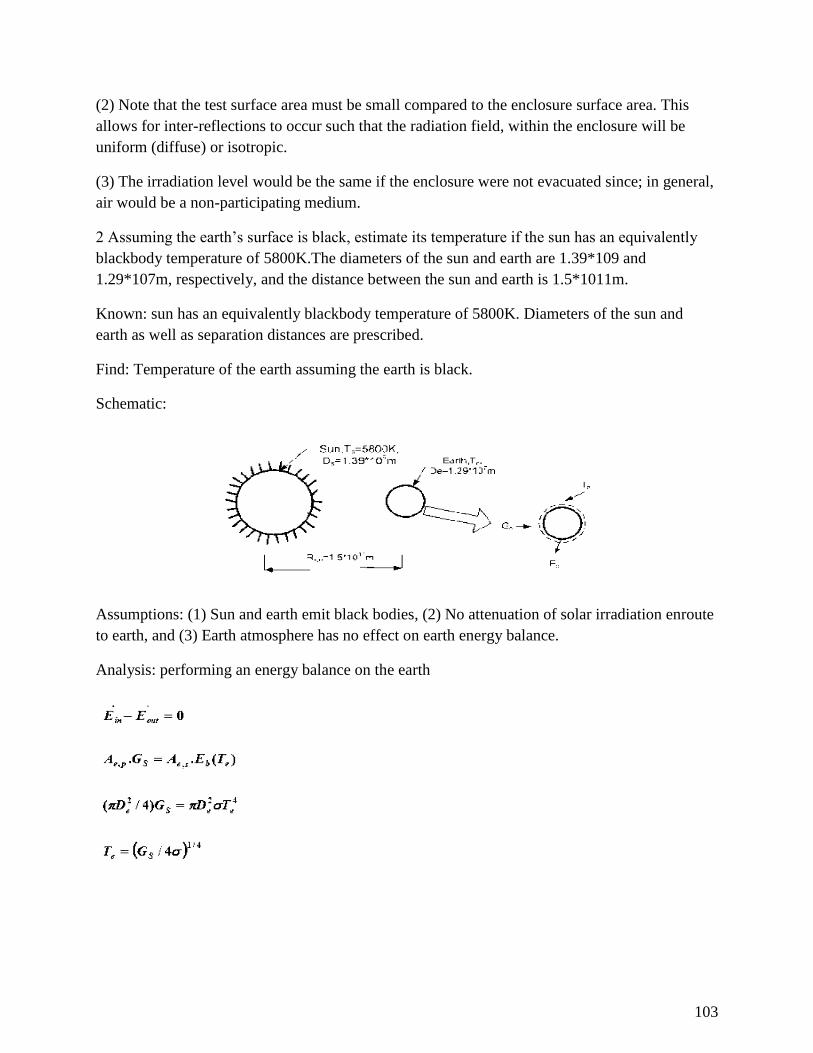
103

(2) Note that the test surface area must be small compared to the enclosure surface area. This

allows for inter-reflections to occur such that the radiation field, within the enclosure will be

uniform (diffuse) or isotropic.

(3) The irradiation level would be the same if the enclosure were not evacuated since; in general,

air would be a non-participating medium.

2 Assuming the earth’s surface is black, estimate its temperature if the sun has an equivalently

blackbody temperature of 5800K.The diameters of the sun and earth are 1.39*109 and

1.29*107m, respectively, and the distance between the sun and earth is 1.5*1011m.

Known: sun has an equivalently blackbody temperature of 5800K. Diameters of the sun and

earth as well as separation distances are prescribed.

Find: Temperature of the earth assuming the earth is black.

Schematic:

Assumptions: (1) Sun and earth emit black bodies, (2) No attenuation of solar irradiation enroute

to earth, and (3) Earth atmosphere has no effect on earth energy balance.

Analysis: performing an energy balance on the earth

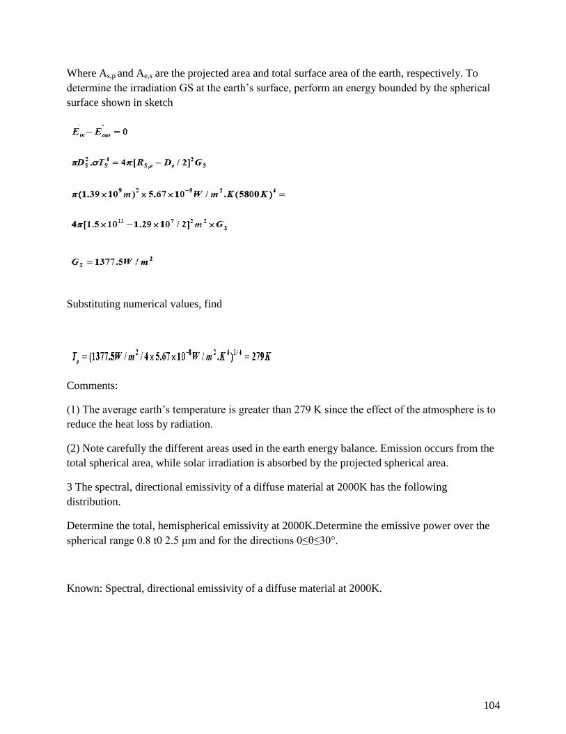
104

Where As,p and Ae,s are the projected area and total surface area of the earth, respectively. To

determine the irradiation GS at the earth’s surface, perform an energy bounded by the spherical

surface shown in sketch

Substituting numerical values, find

Comments:

(1) The average earth’s temperature is greater than 279 K since the effect of the atmosphere is to

reduce the heat loss by radiation.

(2) Note carefully the different areas used in the earth energy balance. Emission occurs from the

total spherical area, while solar irradiation is absorbed by the projected spherical area.

3 The spectral, directional emissivity of a diffuse material at 2000K has the following

distribution.

Determine the total, hemispherical emissivity at 2000K.Determine the emissive power over the

spherical range 0.8 t0 2.5 μm and for the directions 0≤θ≤30°.

Known: Spectral, directional emissivity of a diffuse material at 2000K.

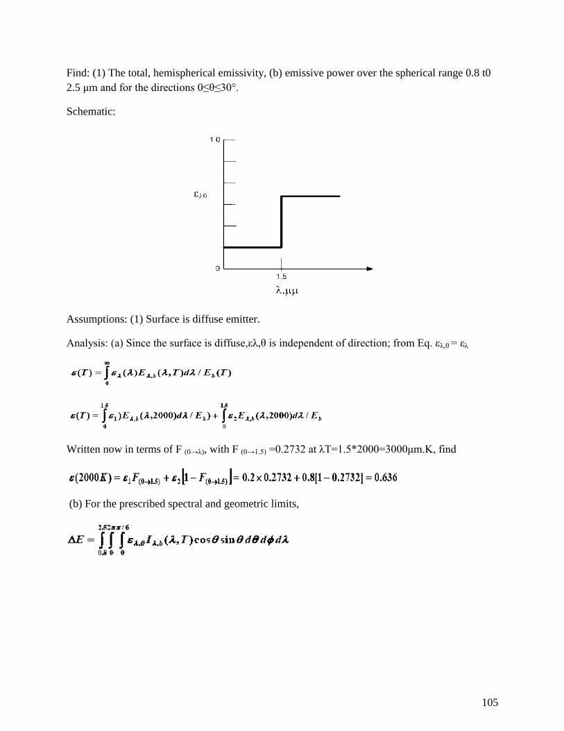
105

Find: (1) The total, hemispherical emissivity, (b) emissive power over the spherical range 0.8 t0

2.5 μm and for the directions 0≤θ≤30°.

Schematic:

Assumptions: (1) Surface is diffuse emitter.

Analysis: (a) Since the surface is diffuse,ελ,θ is independent of direction; from Eq. ελ,θ = ελ

Written now in terms of F (0→λ), with F (0→1.5) =0.2732 at λT=1.5*2000=3000μm.K, find

(b) For the prescribed spectral and geometric limits,

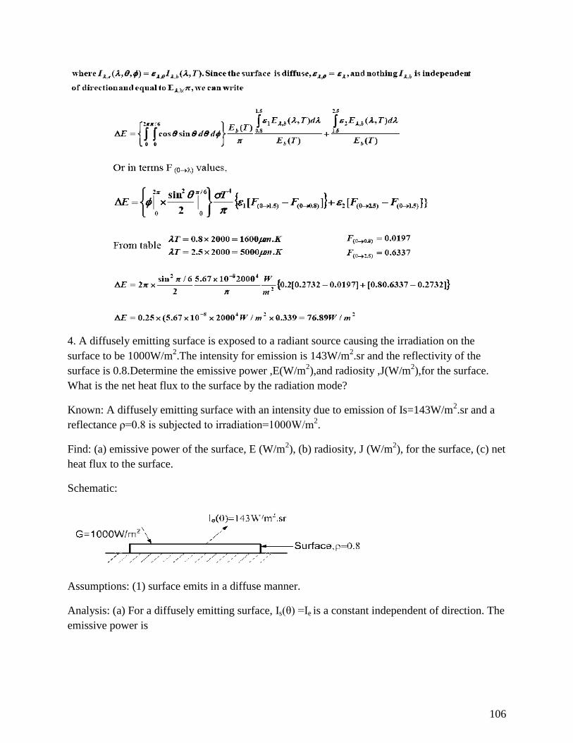
106

4. A diffusely emitting surface is exposed to a radiant source causing the irradiation on the

surface to be 1000W/m2.The intensity for emission is 143W/m

2.sr and the reflectivity of the

surface is 0.8.Determine the emissive power ,E(W/m2),and radiosity ,J(W/m

2),for the surface.

What is the net heat flux to the surface by the radiation mode?

Known: A diffusely emitting surface with an intensity due to emission of Is=143W/m2.sr and a

reflectance ρ=0.8 is subjected to irradiation=1000W/m2.

Find: (a) emissive power of the surface, E (W/m2), (b) radiosity, J (W/m

2), for the surface, (c) net

heat flux to the surface.

Schematic:

Assumptions: (1) surface emits in a diffuse manner.

Analysis: (a) For a diffusely emitting surface, Is(θ) =Ie is a constant independent of direction. The

emissive power is

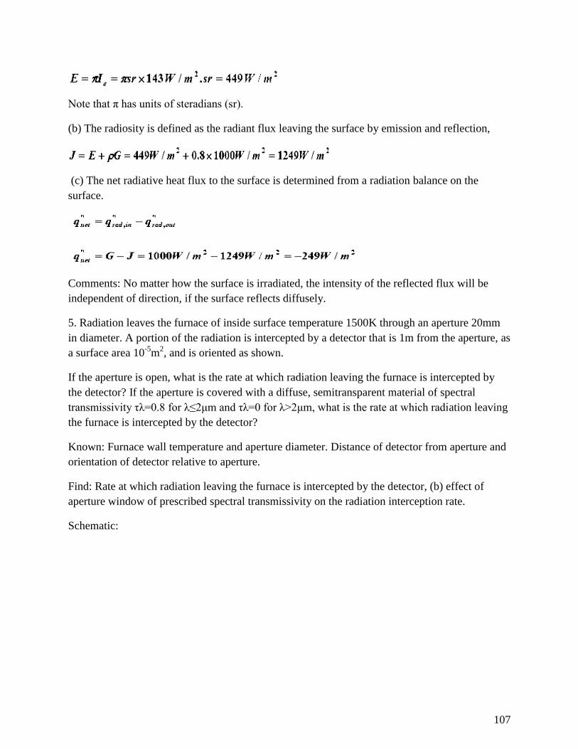
107

Note that π has units of steradians (sr).

(b) The radiosity is defined as the radiant flux leaving the surface by emission and reflection,

(c) The net radiative heat flux to the surface is determined from a radiation balance on the

surface.

Comments: No matter how the surface is irradiated, the intensity of the reflected flux will be

independent of direction, if the surface reflects diffusely.

5. Radiation leaves the furnace of inside surface temperature 1500K through an aperture 20mm

in diameter. A portion of the radiation is intercepted by a detector that is 1m from the aperture, as

a surface area 10-5

m2, and is oriented as shown.

If the aperture is open, what is the rate at which radiation leaving the furnace is intercepted by

the detector? If the aperture is covered with a diffuse, semitransparent material of spectral

transmissivity τλ=0.8 for λ≤2μm and τλ=0 for λ>2μm, what is the rate at which radiation leaving

the furnace is intercepted by the detector?

Known: Furnace wall temperature and aperture diameter. Distance of detector from aperture and

orientation of detector relative to aperture.

Find: Rate at which radiation leaving the furnace is intercepted by the detector, (b) effect of

aperture window of prescribed spectral transmissivity on the radiation interception rate.

Schematic:

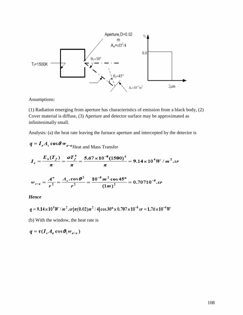
108

Assumptions:

(1) Radiation emerging from aperture has characteristics of emission from a black body, (2)

Cover material is diffuse, (3) Aperture and detector surface may be approximated as

infinitesimally small.

Analysis: (a) the heat rate leaving the furnace aperture and intercepted by the detector is

Heat and Mass Transfer

Hence

(b) With the window, the heat rate is

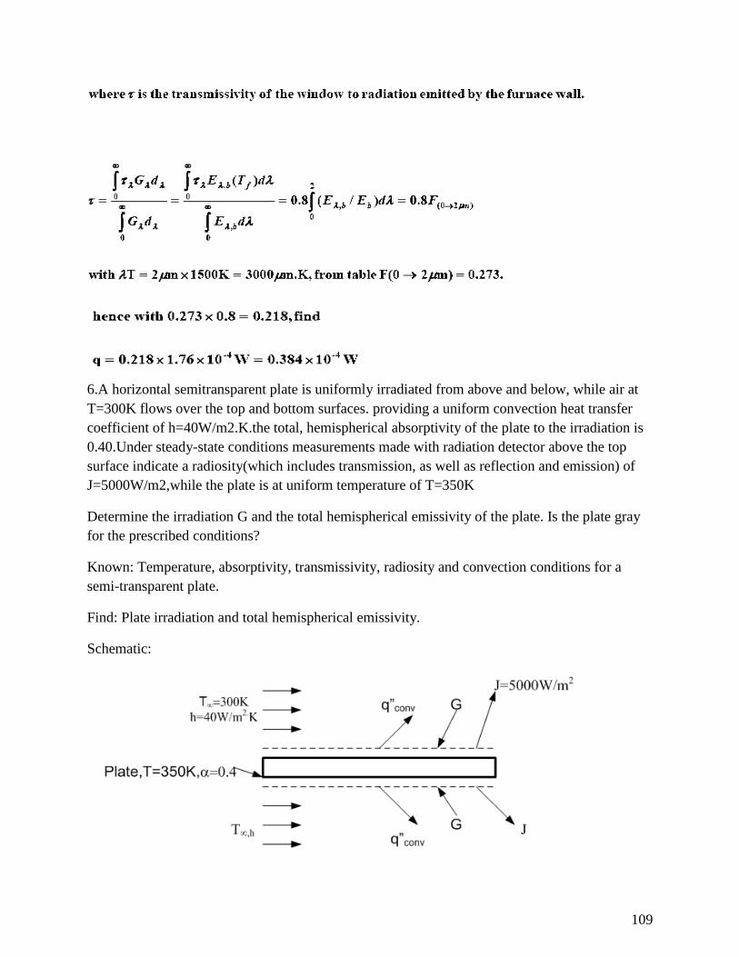
109

6.A horizontal semitransparent plate is uniformly irradiated from above and below, while air at

T=300K flows over the top and bottom surfaces. providing a uniform convection heat transfer

coefficient of h=40W/m2.K.the total, hemispherical absorptivity of the plate to the irradiation is

0.40.Under steady-state conditions measurements made with radiation detector above the top

surface indicate a radiosity(which includes transmission, as well as reflection and emission) of

J=5000W/m2,while the plate is at uniform temperature of T=350K

Determine the irradiation G and the total hemispherical emissivity of the plate. Is the plate gray

for the prescribed conditions?

Known: Temperature, absorptivity, transmissivity, radiosity and convection conditions for a

semi-transparent plate.

Find: Plate irradiation and total hemispherical emissivity.

Schematic:

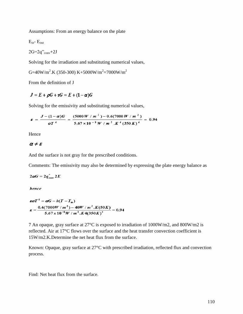
110

Assumptions: From an energy balance on the plate

Ein- Eout

2G=2q”conv+2J

Solving for the irradiation and substituting numerical values,

G=40W/m2.K (350-300) K+5000W/m

2=7000W/m

2

From the definition of J

Solving for the emissivity and substituting numerical values,

Hence

And the surface is not gray for the prescribed conditions.

Comments: The emissivity may also be determined by expressing the plate energy balance as

7 An opaque, gray surface at 27°C is exposed to irradiation of 1000W/m2, and 800W/m2 is

reflected. Air at 17°C flows over the surface and the heat transfer convection coefficient is

15W/m2.K.Determine the net heat flux from the surface.

Known: Opaque, gray surface at 27°C with prescribed irradiation, reflected flux and convection

process.

Find: Net heat flux from the surface.

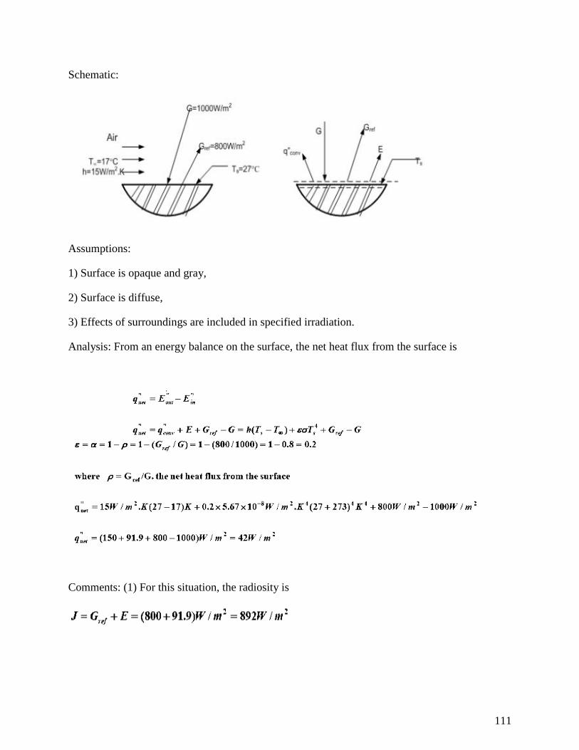
111

Schematic:

Assumptions:

1) Surface is opaque and gray,

2) Surface is diffuse,

3) Effects of surroundings are included in specified irradiation.

Analysis: From an energy balance on the surface, the net heat flux from the surface is

Comments: (1) For this situation, the radiosity is

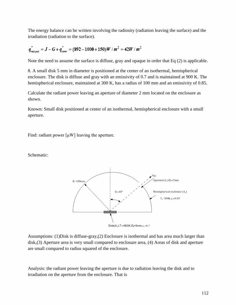
112

The energy balance can be written involving the radiosity (radiation leaving the surface) and the

irradiation (radiation to the surface).

Note the need to assume the surface is diffuse, gray and opaque in order that Eq (2) is applicable.

8. A small disk 5 mm in diameter is positioned at the center of an isothermal, hemispherical

enclosure. The disk is diffuse and gray with an emissivity of 0.7 and is maintained at 900 K. The

hemispherical enclosure, maintained at 300 K, has a radius of 100 mm and an emissivity of 0.85.

Calculate the radiant power leaving an aperture of diameter 2 mm located on the enclosure as

shown.

Known: Small disk positioned at center of an isothermal, hemispherical enclosure with a small

aperture.

Find: radiant power [μW] leaving the aperture.

Schematic:

Assumptions: (1)Disk is diffuse-gray,(2) Enclosure is isothermal and has area much larger than

disk,(3) Aperture area is very small compared to enclosure area, (4) Areas of disk and aperture

are small compared to radius squared of the enclosure.

Analysis: the radiant power leaving the aperture is due to radiation leaving the disk and to

irradiation on the aperture from the enclosure. That is

113

The radiation leaving the disk can be written in terms of the radiosity of the disk. For the diffuse

disk

Combining equations. (2), (3) and (4) into eq.(1) with G2=σT4

3, the radiant power is

114

SCHOOL OF MECHANICAL

DEPARTMENT OF MECHANICAL

UNIT – IV – Heat and Mass Transfer – SMEA1504

115

UNIT IV

Heat Transfer with Change of Phase

4.1 Condensation and Boiling

Heat energy is being converted into electrical energy with the help of water as a

working fluid. Water is first converted into steam when heated in a heat exchanger and then the

exhaust steam coming out of the steam turbine/engine is condensed in a condenser so that the

condensate (water) is recycled again for power generation. Therefore, the condensation and

boiling processes involve heat transfer with change of phase. When a fluid changes its phase, the

magnitude of its properties like density, viscosity, thermal conductivity, specific heat capacity,

etc., change appreciably and the processes taking place are greatly influenced by them. Thus, the

condensation and boiling processes must be well understood for an effective design of different

types of heat exchangers being used in thermal and nuclear power plants, and in process cooling

and heating systems.

4.2 Condensation-Filmwise and Dropwise

Condensation is the process of transition from a vapour to the liquid or solid state. The

process is accompanied by liberation of heat energy due to the change 10 phase. When a vapour

comes 10 contact with a surface maintained at a temperature lower than the saturation

temperature of the vapour corresponding to the pressure at which it exists, the vapour condenses

on the surface and the heat energy thus released has to be removed. The efficiency of the

condensing unit is determined by the mode of condensation that takes place:

Filmwise - the condensing vapour forms a continuous film covering the entire surface,

Dropwise - the vapour condenses into small liquid droplets of various sizes. The

dropwise condensation has a much higher rate of heat transfer than filmwise condensation

because the condensate in dropwise condensation gets removed at a faster rate leading to better

heat transfer between the vapour and the bare surface. .

It is therefore desirable to maintain a condition of dropwise condensation 1D

commercial application. Dropwise condensation can only occur either on highly polished

surfaces or on surfaces contaminated with certain chemicals. Filmwise condensation is expected

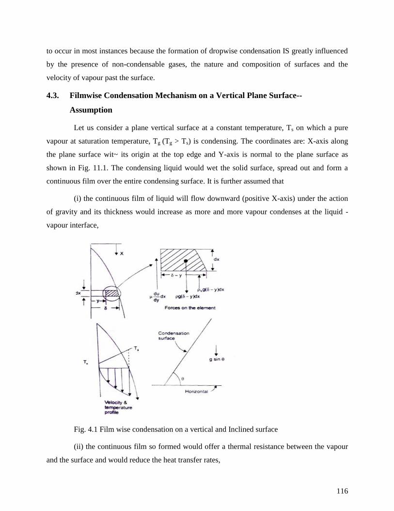
116

to occur in most instances because the formation of dropwise condensation IS greatly influenced

by the presence of non-condensable gases, the nature and composition of surfaces and the

velocity of vapour past the surface.

4.3. Filmwise Condensation Mechanism on a Vertical Plane Surface--

Assumption

Let us consider a plane vertical surface at a constant temperature, Ts on which a pure

vapour at saturation temperature, Tg (Tg > Ts) is condensing. The coordinates are: X-axis along

the plane surface wit~ its origin at the top edge and Y-axis is normal to the plane surface as

shown in Fig. 11.1. The condensing liquid would wet the solid surface, spread out and form a

continuous film over the entire condensing surface. It is further assumed that

(i) the continuous film of liquid will flow downward (positive X-axis) under the action

of gravity and its thickness would increase as more and more vapour condenses at the liquid -

vapour interface,

Fig. 4.1 Film wise condensation on a vertical and Inclined surface

(ii) the continuous film so formed would offer a thermal resistance between the vapour

and the surface and would reduce the heat transfer rates,

117

(iii) the flow in the film would be laminar,

(iv) there would be no shear stress exerted at the liquid vapour interface,

(v) the temperature profile would be linear, and

(vi) the weight of the liquid film would be balanced by the viscous shear in the liquid

film and the buoyant force due to the displaced vapour.

4.4. An Expression for the Liquid Film Thickness and the Heat Transfer

Coefficient in Laminar Filmwise Condensation on a Vertical Plate

We choose a small element, as shown in Fig. 11.1 and by making a force balance, we

write

vg y dx du / dy dx g y dx (5.44)

v is th

liquid, Ii is the thickness of the liquid film at any x, and du/dy is the velocity gradient at x.

Since the no-slip condition requires u = 0 at y = 0, by integration we get:

- v y - y2

(5.45)

And the mass flow rate of condensate through any x position of the film would be

2v

0 0

m u dy g / y y / 2 dy

3v g / 3 (5.46)

The rate of heat transfer at the wall in the area dx is, for unit width,

g sy 0Q kA dt / dy k dx 1 T T /

,

(temperature distribution is linear)

Since the thickness of the film increases in the positive X-direction, an additional mass

of vapour will condense between x and x + dx, i.e.,

118

3 3v vg gd d d

dx dxdx 3 d 3 dx

2

v g d

This additional mass of condensing vapour will release heat energy and that has to

removed by conduction through the wall, or,

2

vfg g s

g dh k dx T T /

(5.47)

We can, therefore, determine the thickness, , of the liquid film by integrating Eq.

(11.4) with the boundary condition: at x = 0, = 0,

or,

0.25

g s

fg v

4 kx T T

gh

(5.48)

The rate of heat transfer is also related by the relation,

g s g sh dx T T k dx T T / ; or, h k /

which can be expressed In dimensionless form in terms of Nusselt number,

0.253

v fg

g s

gh xNu hx / k

4 k T T

(5.49)

The average value of the heat transfer coefficient is obtained by integrating over the

length of the plate:

L

x x

0

h 1/ L h dx 4 / 3 h L

0.253

v fgL

g s

gh LNu 0.943

k T T

(5.50)

The properties of the liquid in Eq. (5.50) and Eq. (5.49) should be evaluated at the mean

119

temperature, T = (Tg + Ts)/2.

Thus:

Local

0.253

v fgx

g s

h x gsinNu 0.707

k T T

and the average

3v fg

L

g s

h L gsinNu 0.943

k T T

(5.51)

These relations should

zero, (a horizontal surface) we would get an absurd result. But these equations are valid for

condensation on the outside surface of vertical tubes as long as the curvature of the tube surface

is not too great.

Solution: (a) Tube Homontal: The mean film temperature is (50 + 76) = 63°C, and the

properties are:

3 3980 kg / m , 0.432 10 Pa s, k 0.66 W / mK

fg vh 2320 kJ / kg,

0.25

2 3fg g sh 0.725 h k g / D T T

0.25

2 33 30.725 980 2320 10 0.66 9.81/ 0.432 10 0.015 26

= 10 kW/m2K

(b) Tube Vertical: Eq (5.50) should be used if the film thickness is very small in

comparison with the tube diameter.

The film thickness, 0.25

g s fg v4 kL T T / gh

120

0.25

2 33

3

980 9.81 2320 10 0.66

0.432 10 1.5 26

= = 0.212 mm << 15.0 mm, the tube diameter.

Therefore, the average heat transfer coefficient would be

0.25 2

v hh h / 0.768 L / D 10 / 2.429 4.11 kW / m K

(Thus, the performance of horizontal tubes for filmwise laminar condensation is much

better than vertical tubes and as such horizontal tubes are preferred.)

Example 4.1A square array of four hundred tubes, 1.5 cm outer diameter is used to condense

steam at atmospheric pressure. The tube walls are maintained at 88°C by a

coolant flowing inside the tubes. Calculate the amount of steam condensed per

hour per unit length of the tubes.

Solution: The properties at the mean temperature (88 + 100)/2 = 94°C are:

-4 Pa-s, k = 0.678 W/mK,

hfg = 2255 × 103 J/kg

A square array of 400 tubes will have N = 20. From Eq (5.57),

0.25

2 3fg g sh 0.725 g k h / N D T T

2 3 3

29.81 963 0.678 2255 100.725 6.328 kW / m K

20 0.000306 0.015 12

Surface area for 400 tubes = 400 × 3.142 × 0.015 × 1 (let L = 1)

= 18.852 m2 per metre length of the tube

Q 852 × 12 = 1431.56 kW

fgm Q / h = 1431.56 × 3600/2255 = 2285.4 kg/hr per metre length.

121

4.5 Condensation inside Tubes-Empirical Relation

The condensation of vapours flowing inside a cylindrical tube is of importance in

chemical and petro-chemical industries. The average heat transfer coefficient for vapours

condensing inside either horizontal or vertical tubes can be determined, within 20 percent

accuracy, by the relations:

For Reg < 5 × 104, Nud = 5.03 (Reg)

1/3 (Pr)

1/3

For Reg > 5 × 104, Nud = 0.0265 (Reg)

0.8 (Pr)

1/3 (5.53)

where Reg is the Reynolds number defined in terms of the mass velocity, or, Reg =

DG/ -sectional area.

4.6 Dropwise Condensation-Merits and Demerits

In dropwise condensation, the condensation is found to appear in t he form 0 f

individual drops. These drops increase in size and combine with another drop until their size is

great enough that their weight causes them to run off the surface and the condensing surface is

exposed for the formation of a new drop. This phenomenon has been observed to occur either on

highly polished surfaces or on surface coated/contaminated with certain fatty acids. The heat

transfer coefficient in dropwise condensation is five to ten times higher than the filmwise

condensation under similar conditions. It is therefore, desirable that conditions should be

maintained for dropwise condensation in commercial applications. The presence of non-

condensable gases, the nature and composition of the surface, the vapour velocity past the

surface have great influence on the formation of drops on coated/contaminated surfaces and It is

rather difficult to achieve dr0pwlse condensation.

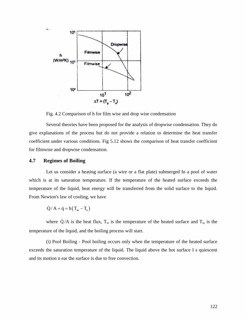
122

Fig. 4.2 Comparison of h for film wise and drop wise condensation

Several theories have been proposed for the analysis of dropwise condensation. They do

give explanations of the process but do not provide a relation to determine the heat transfer

coefficient under various conditions. Fig 5.12 shows the comparison of heat transfer coefficient

for filmwise and dropwise condensation.

4.7 Regimes of Boiling

Let us consider a heating surface (a wire or a flat plate) submerged In a pool of water

which is at its saturation temperature. If the temperature of the heated surface exceeds the

temperature of the liquid, heat energy will be transferred from the solid surface to the liquid.

From Newton's law of cooling, we have

w sQ / A q h T T

where Q /A is the heat flux, Tw is the temperature of the heated surface and Ts, is the

temperature of the liquid, and the boiling process will start.

(i) Pool Boiling - Pool boiling occurs only when the temperature of the heated surface

exceeds the saturation temperature of the liquid. The liquid above the hot surface I s quiescent

and its motion n ear the surface is due to free convection.

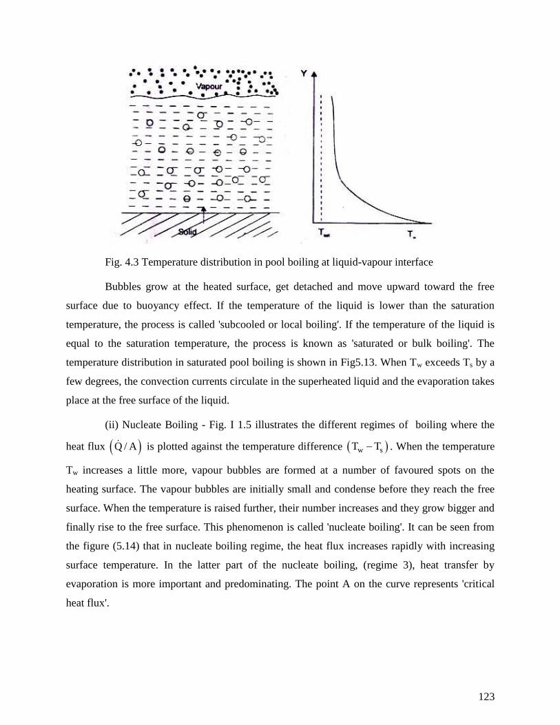
123

Fig. 4.3 Temperature distribution in pool boiling at liquid-vapour interface

Bubbles grow at the heated surface, get detached and move upward toward the free

surface due to buoyancy effect. If the temperature of the liquid is lower than the saturation

temperature, the process is called 'subcooled or local boiling'. If the temperature of the liquid is

equal to the saturation temperature, the process is known as 'saturated or bulk boiling'. The

temperature distribution in saturated pool boiling is shown in Fig5.13. When Tw exceeds Ts by a

few degrees, the convection currents circulate in the superheated liquid and the evaporation takes

place at the free surface of the liquid.

(ii) Nucleate Boiling - Fig. I 1.5 illustrates the different regimes of boiling where the

heat flux Q / A is plotted against the temperature difference w sT T . When the temperature

Tw increases a little more, vapour bubbles are formed at a number of favoured spots on the

heating surface. The vapour bubbles are initially small and condense before they reach the free

surface. When the temperature is raised further, their number increases and they grow bigger and

finally rise to the free surface. This phenomenon is called 'nucleate boiling'. It can be seen from

the figure (5.14) that in nucleate boiling regime, the heat flux increases rapidly with increasing

surface temperature. In the latter part of the nucleate boiling, (regime 3), heat transfer by

evaporation is more important and predominating. The point A on the curve represents 'critical

heat flux'.

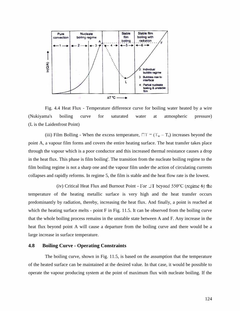
124

Fig. 4.4 Heat Flux - Temperature difference curve for boiling water heated by a wire

(Nukiyama's boiling curve for saturated water at atmospheric pressure)

(L is the Laidenfrost Point)

(iii) Film Bolling - When the excess temperature, w – Ts) increases beyond the

point A, a vapour film forms and covers the entire heating surface. The heat transfer takes place

through the vapour which is a poor conductor and this increased thermal resistance causes a drop

in the heat flux. This phase is film boiling'. The transition from the nucleate boiling regime to the

film boiling regime is not a sharp one and the vapour film under the action of circulating currents

collapses and rapidly reforms. In regime 5, the film is stable and the heat flow rate is the lowest.

(iv) Critical Heat Flux and Burnout Point -

temperature of the heating metallic surface is very high and the heat transfer occurs

predominantly by radiation, thereby, increasing the heat flux. And finally, a point is reached at

which the heating surface melts - point F in Fig. 11.5. It can be observed from the boiling curve

that the whole boiling process remains in the unstable state between A and F. Any increase in the

heat flux beyond point A will cause a departure from the boiling curve and there would be a

large increase in surface temperature.

4.8 Boiling Curve - Operating Constraints

The boiling curve, shown in Fig. 11.5, is based on the assumption that the temperature

of the heated surface can be maintained at the desired value. In that case, it would be possible to

operate the vapour producing system at the point of maximum flux with nucleate boiling. If the

125

heat flux instead of the surface temperature, is the independent variable and it IS desired to

operate the system at the point of maximum flux, it is just possible that a slight increase in the

heat flux will increase the surface temperature substantially. And, the equilibrium will be

established at point F. If the material of the heating element has its melting point temperature

lower than the temperature at the equilibrium point F, the heating element will melt.

4.9 Factors Affecting Nucleate Boiling

Since high heat transfer rates and convection coefficients are associated with small values of the

excess temperature, it is desirable that many engineering devices operate in the nucleate boiling

regime. It is possible to get heat transfer coefficients in excess of 104 W/m

2 in nucleate boiling

regime and these values are substantially larger than those normally obtained in convection

processes with no phase change. The factors which affect the nucleate boiling are:

(a) Pressure - Pressure controls the rate of bubble growth and therefore affects the

temperature difference causing the heat energy to flow. The maximum allowable heat flux for a

boiling liquid first increases with pressure until critical pressure is reached and then decreases.

(b) Heating Surface Characteristics - The material of the heating element has a

significant effect on the boiling heat transfer coefficient. Copper has a higher value than

chromium, steel and zinc. Further, a rough surface gives a better heat transfer rate than a smooth

or coated surface, because a rough surface gets wet more easily than a smooth one.

(c) Thermo-mechanical Properties of Liquids - A higher thermal conductivity of the

liquid will cause higher heat transfer rates and the viscosity and surface tension will have a

marked effect on the bubble size and their rate of formation which affects the rate of heat

transfer.

(d) Mechanical Agitation - The rate of heat transfer will increase with the increasing

degree of mechanical agitation. Forced convection increases mixing of bubbles and the rate of

heat transfer.

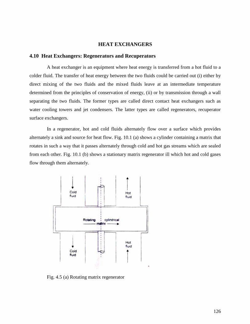
126

HEAT EXCHANGERS

4.10 Heat Exchangers: Regenerators and Recuperators

A heat exchanger is an equipment where heat energy is transferred from a hot fluid to a

colder fluid. The transfer of heat energy between the two fluids could be carried out (i) either by

direct mixing of the two fluids and the mixed fluids leave at an intermediate temperature

determined from the principles of conservation of energy, (ii) or by transmission through a wall

separating the two fluids. The former types are called direct contact heat exchangers such as

water cooling towers and jet condensers. The latter types are called regenerators, recuperator

surface exchangers.

In a regenerator, hot and cold fluids alternately flow over a surface which provides

alternately a sink and source for heat flow. Fig. 10.1 (a) shows a cylinder containing a matrix that

rotates in such a way that it passes alternately through cold and hot gas streams which are sealed

from each other. Fig. 10.1 (b) shows a stationary matrix regenerator ill which hot and cold gases

flow through them alternately.

Fig. 4.5 (a) Rotating matrix regenerator

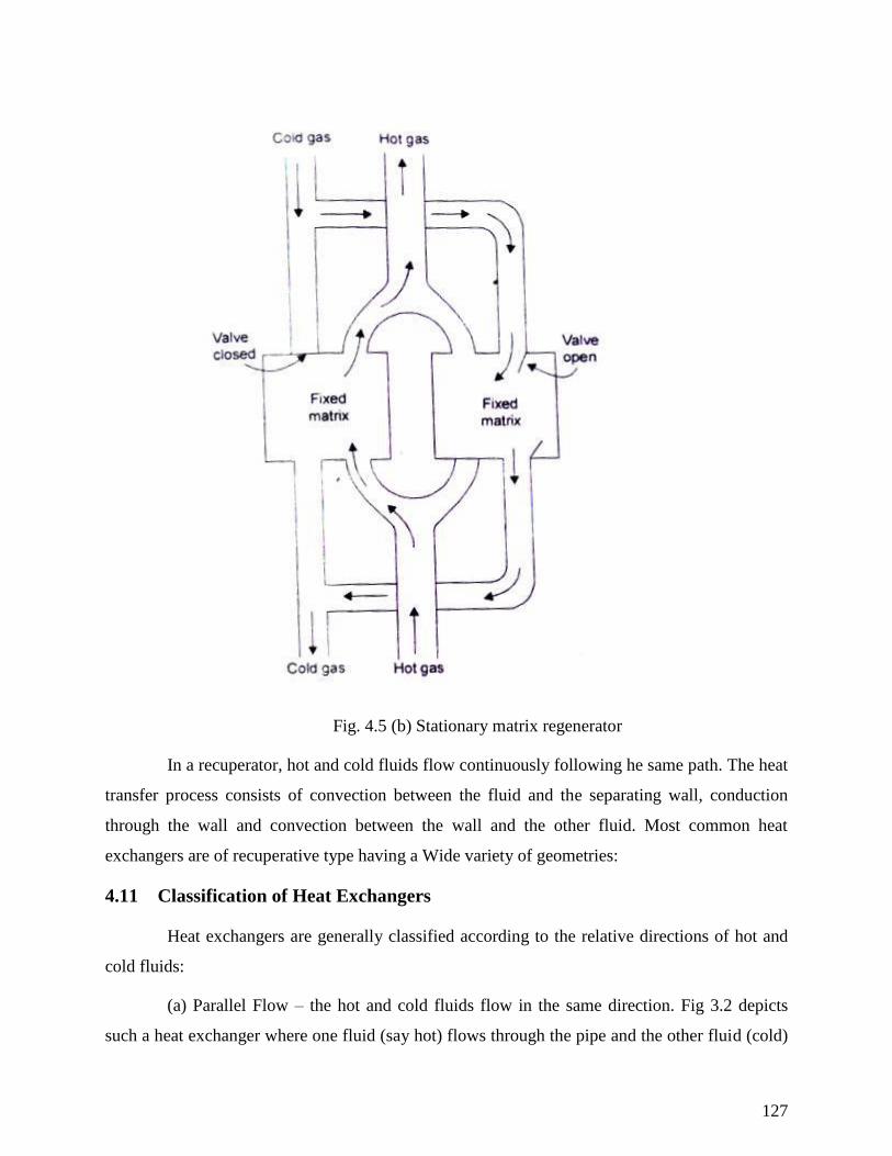
127

Fig. 4.5 (b) Stationary matrix regenerator

In a recuperator, hot and cold fluids flow continuously following he same path. The heat

transfer process consists of convection between the fluid and the separating wall, conduction

through the wall and convection between the wall and the other fluid. Most common heat

exchangers are of recuperative type having a Wide variety of geometries:

4.11 Classification of Heat Exchangers

Heat exchangers are generally classified according to the relative directions of hot and

cold fluids:

(a) Parallel Flow – the hot and cold fluids flow in the same direction. Fig 3.2 depicts

such a heat exchanger where one fluid (say hot) flows through the pipe and the other fluid (cold)

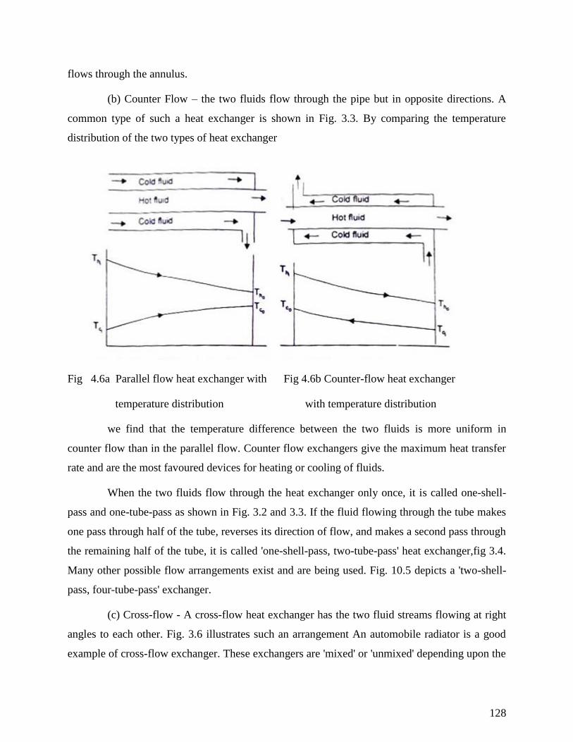
128

flows through the annulus.

(b) Counter Flow – the two fluids flow through the pipe but in opposite directions. A

common type of such a heat exchanger is shown in Fig. 3.3. By comparing the temperature

distribution of the two types of heat exchanger

Fig 4.6a Parallel flow heat exchanger with Fig 4.6b Counter-flow heat exchanger

temperature distribution with temperature distribution

we find that the temperature difference between the two fluids is more uniform in

counter flow than in the parallel flow. Counter flow exchangers give the maximum heat transfer

rate and are the most favoured devices for heating or cooling of fluids.

When the two fluids flow through the heat exchanger only once, it is called one-shell-

pass and one-tube-pass as shown in Fig. 3.2 and 3.3. If the fluid flowing through the tube makes

one pass through half of the tube, reverses its direction of flow, and makes a second pass through

the remaining half of the tube, it is called 'one-shell-pass, two-tube-pass' heat exchanger,fig 3.4.

Many other possible flow arrangements exist and are being used. Fig. 10.5 depicts a 'two-shell-

pass, four-tube-pass' exchanger.

(c) Cross-flow - A cross-flow heat exchanger has the two fluid streams flowing at right

angles to each other. Fig. 3.6 illustrates such an arrangement An automobile radiator is a good

example of cross-flow exchanger. These exchangers are 'mixed' or 'unmixed' depending upon the

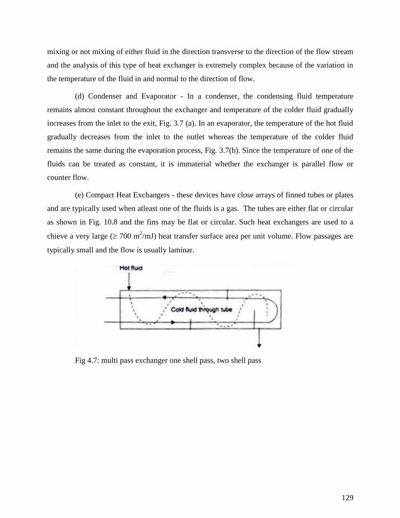
129

mixing or not mixing of either fluid in the direction transverse to the direction of the flow stream

and the analysis of this type of heat exchanger is extremely complex because of the variation in

the temperature of the fluid in and normal to the direction of flow.

(d) Condenser and Evaporator - In a condenser, the condensing fluid temperature

remains almost constant throughout the exchanger and temperature of the colder fluid gradually

increases from the inlet to the exit, Fig. 3.7 (a). In an evaporator, the temperature of the hot fluid

gradually decreases from the inlet to the outlet whereas the temperature of the colder fluid

remains the same during the evaporation process, Fig. 3.7(b). Since the temperature of one of the

fluids can be treated as constant, it is immaterial whether the exchanger is parallel flow or

counter flow.

(e) Compact Heat Exchangers - these devices have close arrays of finned tubes or plates

and are typically used when atleast one of the fluids is a gas. The tubes are either flat or circular

as shown in Fig. 10.8 and the fins may be flat or circular. Such heat exchangers are used to a

chieve a very large ( 700 m2/mJ) heat transfer surface area per unit volume. Flow passages are

typically small and the flow is usually laminar.

Fig 4.7: multi pass exchanger one shell pass, two shell pass

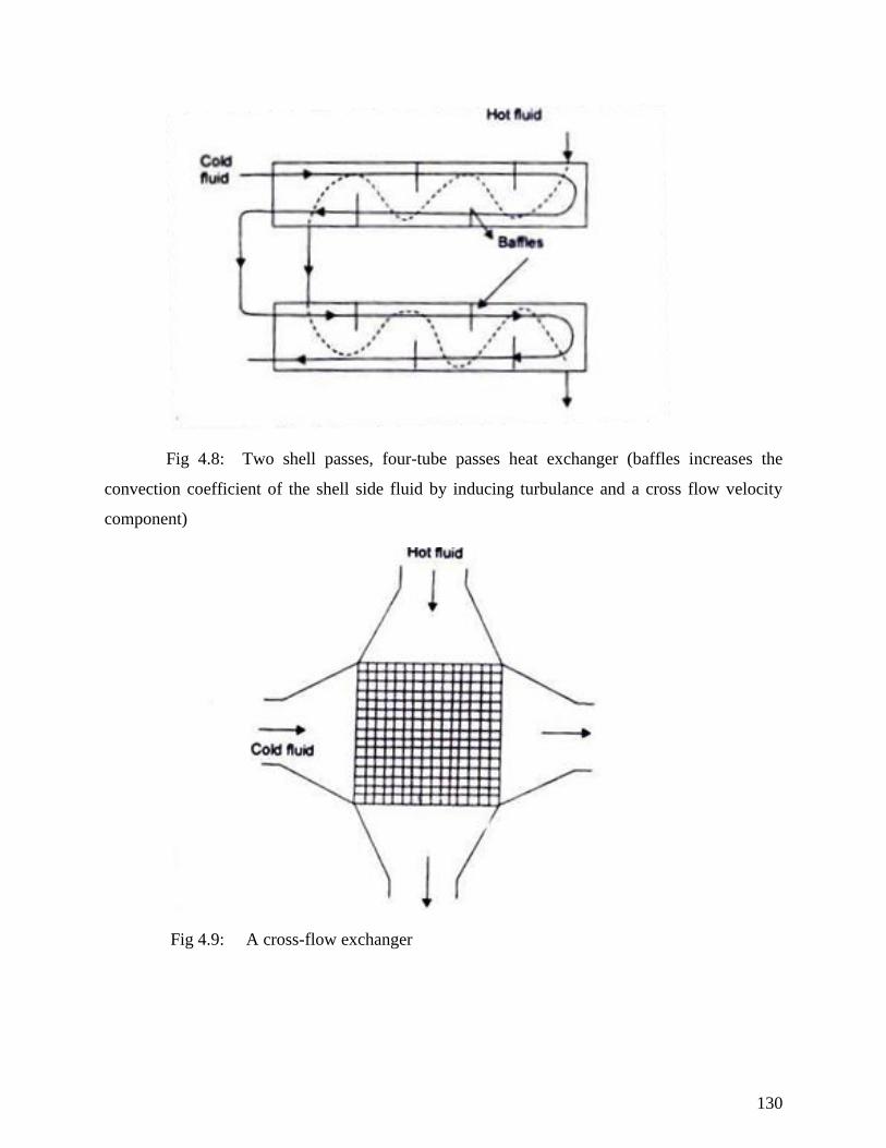
130

Fig 4.8: Two shell passes, four-tube passes heat exchanger (baffles increases the

convection coefficient of the shell side fluid by inducing turbulance and a cross flow velocity

component)

Fig 4.9: A cross-flow exchanger

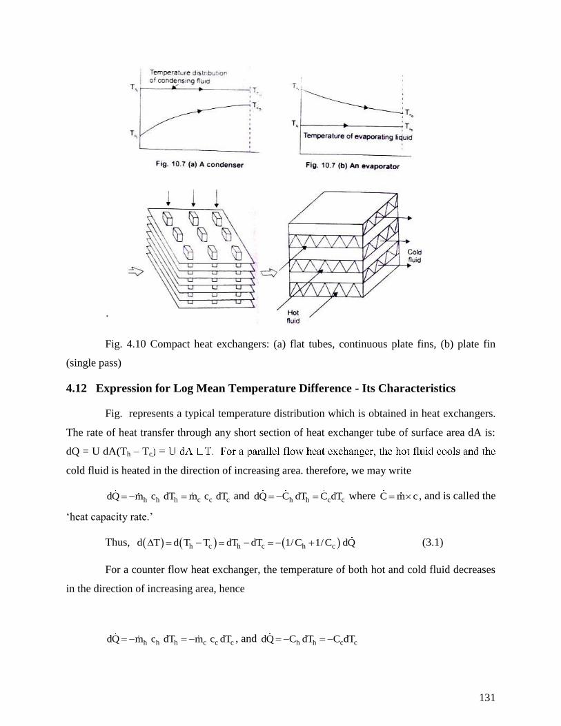
131

Fig. 4.10 Compact heat exchangers: (a) flat tubes, continuous plate fins, (b) plate fin

(single pass)

4.12 Expression for Log Mean Temperature Difference - Its Characteristics

Fig. represents a typical temperature distribution which is obtained in heat exchangers.

The rate of heat transfer through any short section of heat exchanger tube of surface area dA is:

dQ = U dA(Th – Tc

cold fluid is heated in the direction of increasing area. therefore, we may write

h h h c c cdQ m c dT m c dT and h h c cdQ C dT C dT where C m c , and is called the

‘heat capacity rate.’

Thus, h c h c h cd T d T T dT dT 1/C 1/C dQ (3.1)

For a counter flow heat exchanger, the temperature of both hot and cold fluid decreases

in the direction of increasing area, hence

h h h c c cdQ m c dT m c dT , and h h c cdQ C dT C dT

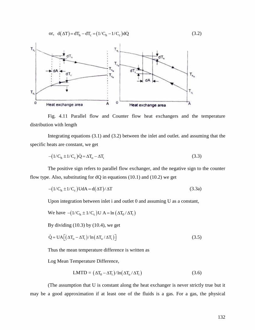
132

or, h c h cd T dT dT 1/C 1/C dQ (3.2)

Fig. 4.11 Parallel flow and Counter flow heat exchangers and the temperature

distribution with length

Integrating equations (3.1) and (3.2) between the inlet and outlet. and assuming that the

specific heats are constant, we get

h c o i1/C 1/C Q T T (3.3)

The positive sign refers to parallel flow exchanger, and the negative sign to the counter

flow type. Also, substituting for dQ in equations (10.1) and (10.2) we get

h c1/C 1/C UdA d T / T (3.3a)

Upon integration between inlet i and outlet 0 and assuming U as a constant,

We have h c 0 i1/C 1/C U A ln T / T

By dividing (10.3) by (10.4), we get

o i o iQ UA T T / ln T / T (3.5)

Thus the mean temperature difference is written as

Log Mean Temperature Difference,

LMTD = 0 i o iT T / ln T / T (3.6)

(The assumption that U is constant along the heat exchanger is never strictly true but it

may be a good approximation if at least one of the fluids is a gas. For a gas, the physical

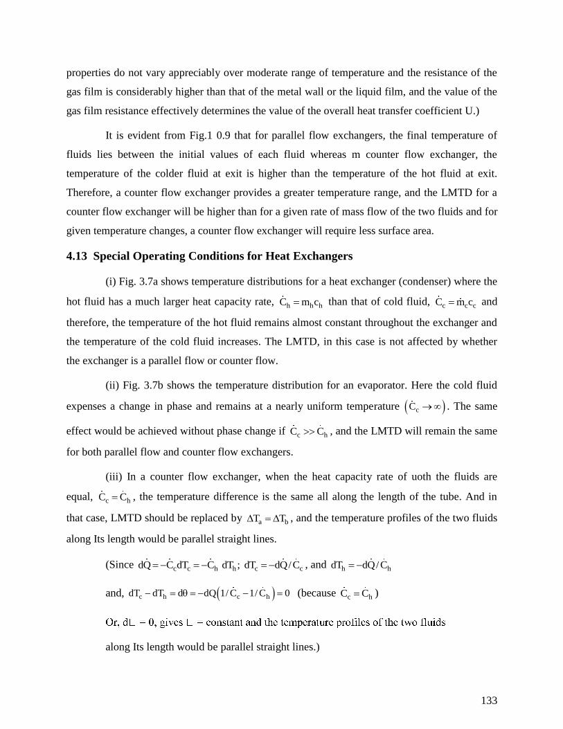
133

properties do not vary appreciably over moderate range of temperature and the resistance of the

gas film is considerably higher than that of the metal wall or the liquid film, and the value of the

gas film resistance effectively determines the value of the overall heat transfer coefficient U.)

It is evident from Fig.1 0.9 that for parallel flow exchangers, the final temperature of

fluids lies between the initial values of each fluid whereas m counter flow exchanger, the

temperature of the colder fluid at exit is higher than the temperature of the hot fluid at exit.

Therefore, a counter flow exchanger provides a greater temperature range, and the LMTD for a

counter flow exchanger will be higher than for a given rate of mass flow of the two fluids and for

given temperature changes, a counter flow exchanger will require less surface area.

4.13 Special Operating Conditions for Heat Exchangers

(i) Fig. 3.7a shows temperature distributions for a heat exchanger (condenser) where the

hot fluid has a much larger heat capacity rate, h h hC m c than that of cold fluid, c c cC m c and

therefore, the temperature of the hot fluid remains almost constant throughout the exchanger and

the temperature of the cold fluid increases. The LMTD, in this case is not affected by whether

the exchanger is a parallel flow or counter flow.

(ii) Fig. 3.7b shows the temperature distribution for an evaporator. Here the cold fluid

expenses a change in phase and remains at a nearly uniform temperature cC . The same

effect would be achieved without phase change if c hC C , and the LMTD will remain the same

for both parallel flow and counter flow exchangers.

(iii) In a counter flow exchanger, when the heat capacity rate of uoth the fluids are

equal, c hC C , the temperature difference is the same all along the length of the tube. And in

that case, LMTD should be replaced by a bT T , and the temperature profiles of the two fluids

along Its length would be parallel straight lines.

(Since c c h h c cdQ C dT C dT ; dT dQ/C , and h hdT dQ/C

and, c h c hdT dT d dQ 1/ C 1/ C 0 (because c hC C )

along Its length would be parallel straight lines.)

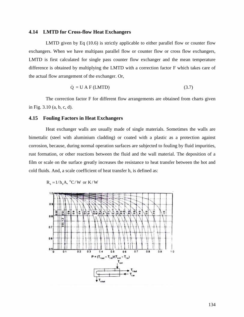
134

4.14 LMTD for Cross-flow Heat Exchangers

LMTD given by Eq (10.6) is strictly applicable to either parallel flow or counter flow

exchangers. When we have multipass parallel flow or counter flow or cross flow exchangers,

LMTD is first calculated for single pass counter flow exchanger and the mean temperature

difference is obtained by multiplying the LMTD with a correction factor F which takes care of

the actual flow arrangement of the exchanger. Or,

Q = U A F (LMTD) (3.7)

The correction factor F for different flow arrangements are obtained from charts given

in Fig. 3.10 (a, b, c, d).

4.15 Fouling Factors in Heat Exchangers

Heat exchanger walls are usually made of single materials. Sometimes the walls are

bimettalic (steel with aluminium cladding) or coated with a plastic as a protection against

corrosion, because, during normal operation surfaces are subjected to fouling by fluid impurities,

rust formation, or other reactions between the fluid and the wall material. The deposition of a

film or scale on the surface greatly increases the resistance to heat transfer between the hot and

cold fluids. And, a scale coefficient of heat transfer h, is defined as:

os sR 1/ h A, C/ W or K/ W

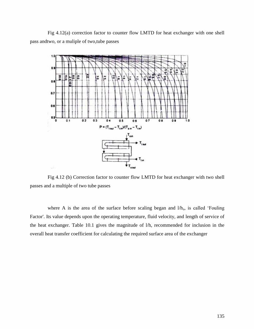
135

Fig 4.12(a) correction factor to counter flow LMTD for heat exchanger with one shell

pass andtwo, or a muliple of two,tube passes

Fig 4.12 (b) Correction factor to counter flow LMTD for heat exchanger with two shell

passes and a multiple of two tube passes

where A is the area of the surface before scaling began and l/hs, is called ‘Fouling

Factor'. Its value depends upon the operating temperature, fluid velocity, and length of service of

the heat exchanger. Table 10.1 gives the magnitude of l/h, recommended for inclusion in the

overall heat transfer coefficient for calculating the required surface area of the exchanger

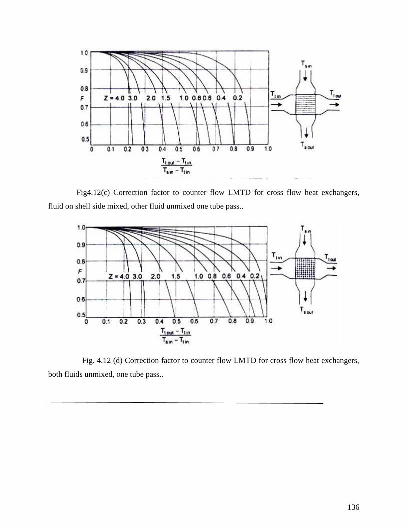
136

Fig4.12(c) Correction factor to counter flow LMTD for cross flow heat exchangers,

fluid on shell side mixed, other fluid unmixed one tube pass..

Fig. 4.12 (d) Correction factor to counter flow LMTD for cross flow heat exchangers,

both fluids unmixed, one tube pass..

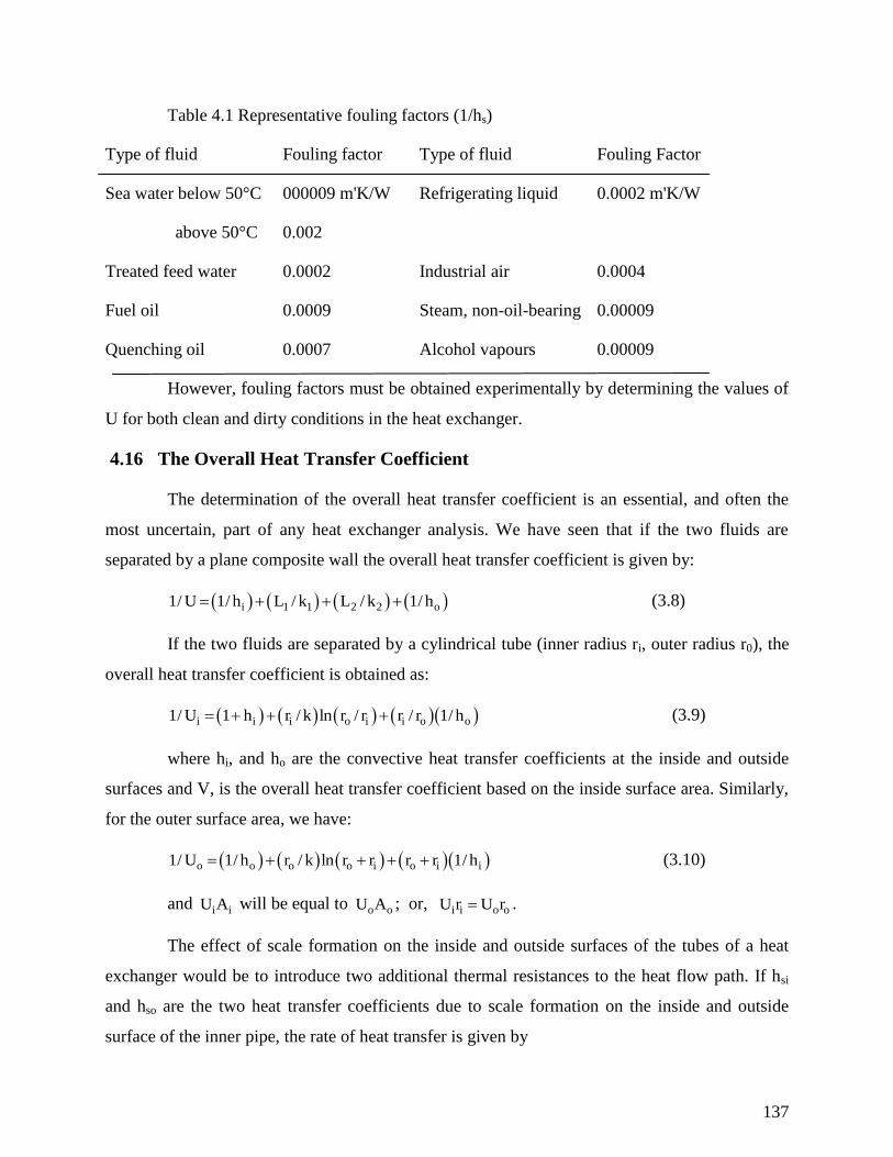
137

Table 4.1 Representative fouling factors (1/hs)

Type of fluid Fouling factor Type of fluid Fouling Factor

Sea water below 50°C 000009 m'K/W Refrigerating liquid 0.0002 m'K/W

above 50°C 0.002

Treated feed water 0.0002 Industrial air 0.0004

Fuel oil 0.0009 Steam, non-oil-bearing 0.00009

Quenching oil 0.0007 Alcohol vapours 0.00009

However, fouling factors must be obtained experimentally by determining the values of

U for both clean and dirty conditions in the heat exchanger.

4.16 The Overall Heat Transfer Coefficient

The determination of the overall heat transfer coefficient is an essential, and often the

most uncertain, part of any heat exchanger analysis. We have seen that if the two fluids are

separated by a plane composite wall the overall heat transfer coefficient is given by:

i 1 1 2 2 o1/ U 1/ h L / k L / k 1/ h (3.8)

If the two fluids are separated by a cylindrical tube (inner radius ri, outer radius r0), the

overall heat transfer coefficient is obtained as:

i i i o i i o o1/ U 1 h r / k ln r / r r / r 1/ h (3.9)

where hi, and ho are the convective heat transfer coefficients at the inside and outside

surfaces and V, is the overall heat transfer coefficient based on the inside surface area. Similarly,

for the outer surface area, we have:

o o o o i o i i1/ U 1/ h r / k ln r r r r 1/ h (3.10)

and i iU A will be equal to o oU A ; or, i i o oU r U r .

The effect of scale formation on the inside and outside surfaces of the tubes of a heat

exchanger would be to introduce two additional thermal resistances to the heat flow path. If hsi

and hso are the two heat transfer coefficients due to scale formation on the inside and outside

surface of the inner pipe, the rate of heat transfer is given by

138

i o i i si i o i so o o oQ T T / 1/ h A 1/ h A ln r r / 2 Lk 1/ h A 1/ h A (3.11)

where Ti, and To are the temperature of the fluid at the inside and outside of the tube.

Thus, the overall heat transfer coeffiCIent based on the inside and outside surface area of the

tube would be:

i i si i o i i o so i o o1/ U 1/ h 1/ h r / k ln r / r r / r 1/ h r / r 1/ h ; (3.12)

and

o o i i o i si o i 0 so o1/ U r / r 1/ h r / r 1/ h ln r / r r / k 1/ h 1/ h

Example 4.1 In a parallel flow heat exchanger water flows through the inner pipe and is heated

from 25°C to 75°C. Oil flowing through the annulus is cooled from 210°C to

110°C. It is desired to cool the oil to a lower temperature by increasing the length

of the tube. Estimate the minimum temperature to which the oil can be cooled.

Solution: By making an energy balance, heat received by water must be equal to 4he

heat given out by oil.

w w o o w om c 75 25 m c 210 110 ;C /C 100/50 2.0

In a parallel flow heat exchanger, the minimum temperature to which oil can be cooled

will be equal to the maximum temperature to which water can be heated,

Fig. 10.2: ho coT T

therefore, Cw (T –25) = Co (210 – T);

(T – 25)/(210 – T) = 1/2 = 0.5; or, T = 260/3 = 86.67°C.

or the same capacity rates the oil can be cooled to 25°C (equal to the water inlet

temperature) in a counter-flow arrangement.

Example 4.2 Water at the rate of 1.5 kg/s IS heated from 30°C to 70°C by an oil (specific heat

1.95 kJ/kg C). Oil enters the exchanger at 120°C and leaves the exchanger at

80°C. If the overall heat transfer coefficient remains constant at 350 W /m2°C,

calculate the heat exchange area for (i) parallel-flow, (ii) counter-flow, and (iii)

cross-flow arrangement.

139

Solution: Energy absorbed by water,

w wQ m c T 1.5 4.182 40 250.92 kW

(i) Parallel flow: Fig. 10.9; a bT 120 30 90; T 80 70 10

LMTD = (90 – 10)/ln(90/10) = 36.4;

Area = Q/U (LMTD) = 250920 /(350 × 36.4) = 19.69 m2.

(ii) Coun a. = 120 – b = 80 – 30 = 50

a b

Area A = 2Q / U T 250920 / 350 50 14.33 m

(iii) Cross flow: assuming both fluids unmixed - Fig. 10.10d

using the nomenclature of the figure and assuming that water flows through the tubes

and oil flows through the shell,

to ti si tiP T T / T T 70 30 / 120 30 0.444

si so to tiZ T T / T T 120 80 / 70 30 1.0

and the correction factor, F = 0.93

Q UAF T ; or Area A = 250920/(350 × 0.93 × 50) = 15.41 m2.

Example 4.3 0.5 kg/s of exhaust gases flowing through a heat exchanger are cooled from

400°C to 120°C by water initially at 25°C. The specific heat capacities of exhaust

gases and water are 1.15 and 4.19 kJ/kgK respectively, and the overall heat

transfer coefficient from gases to water is 150 W/m2K. If the cooling water flow

rate is 0.7 kg/s, calculate the surface area when (i) parallel-flow (ii) cross-flow

with exhaust gases flowing through tubes and water is mixed in the shell.

Solution: The heat given out by the exhaust gases is equal to the heat gained by water.

140

or, 0.5 × 1.15 × (400 – 120) = 0.7 × 4.19 × (T – 25)

Therefore, the temperature of water at exit, T = 79.89°C

For paralle1-flow: aT 400 25 375; bT 120 79.89 40.11

LMID = (375 – 40.11)/ln(375/40.11) = 149.82

Q = 0.5 × 1.15 × 280 = 161000 W;

Therefore Area A = 161000/(150 × 149.82) = 7.164 m2

For cross-flow: Q = U A F (LMTD);

and LMTD is calculated for counter-flow system.

a bT 400 79.89 320.11; T 120 25 95

LMTD = 320.11 95 / ln 320.11/ 95 185.3

Using the nomenclature of Fig 10.10c,

P 120 400 / 25 400 0.747

Z 25 79.89 / 120 400 0.196 F 0.92

and the area 2A 161000 / 150 0.92 185.3 6.296 m

Example 4.4 In a certain double pipe heat exchanger hot water flows at a rate of 5000 kg/h and

gets cooled from 95°C to 65°C. At the same time 5000 kg/h of cooling water enters

the heat exchanger. The overall heat transfer coefficient is 2270 W/m2K. Calculate

the heat transfer area and the efficiency assuming two streams are in (i) parallel

flow (ii) counter flow. Take Cp for water as 4.2 kJ/kgK, cooling water inlet

temperature 30°C.

Solution: By making an energy balance:

Heat lost by hot water = 5000 ×4.2 ×(95 –65)

= heat gained by cold water = 5000 ×4.2 ×(T –30) 30

T = 60oC

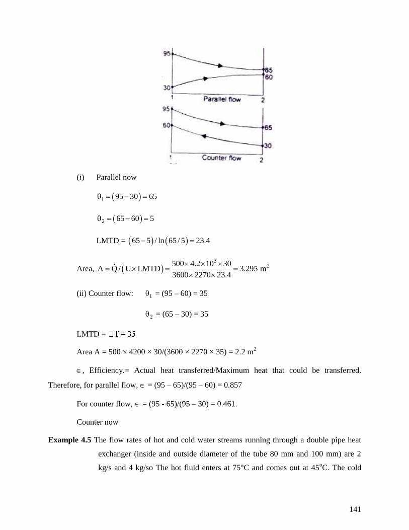
141

(i) Parallel now

1 95 30 65

2 65 60 5

LMTD = 65 5 / ln 65 / 5 23.4

Area, 3

2500 4.2 10 30A Q / U LMTD 3.295 m

3600 2270 23.4

(ii) Counter flow: 1 = (95 – 60) = 35

2 = (65 – 30) = 35

LMTD =

Area A = 500 × 4200 × 30/(3600 × 2270 × 35) = 2.2 m2

, Efficiency.= Actual heat transferred/Maximum heat that could be transferred.

Therefore, for parallel flow, = (95 – 65)/(95 – 60) = 0.857

For counter flow, = (95 - 65)/(95 – 30) = 0.461.

Counter now

Example 4.5 The flow rates of hot and cold water streams running through a double pipe heat

exchanger (inside and outside diameter of the tube 80 mm and 100 mm) are 2

kg/s and 4 kg/so The hot fluid enters at 75°C and comes out at 45oC. The cold

142

fluid enters at 20°C. If the convective heat transfer at the inside and outside

surface of the tube is 150 and 180 W /m2K, thermal conductivity of the tube

material 40 W/mK, calculate the area of the heat exchanger assuming counter

flow.

Solution: Let T is the temperature of the cold water at outlet.

By making an energy balance, h h h1 h2 c c c2 c1Q m c T T m c T T

since oh cc c , 4.2 kJ / kgK; 2 75 45 4 T 20 ; T 35 C

and Q 252 kW

for counter flow: 1 275 35 40; 45 20 25

LMTD = (40 – 25) / ln (40/25) = 31.91

overall heat transfer coefficient based in the inside surface of tube

i i o i o i o1/ U 1/ h r / k ln r / r r r 1/ h

1/150 0.04 / 40 ln 50 / 40 50 / 40 1/180 0.0138

and U = 72.28

area 3 2A Q / U LMTD 252 10 / 72.28 31.91 109.26 m

Example 4.6 Water flows through a copper tube (k = 350 W/mK, inner and outer diameter

2.0 cm and 2.5 cm respectively) of a double pipe heat exchanger. Oil flows

through the annulus between this pipe and steel pipe. The convective heat

transfer coefficient on the inside and outside of the copper tube are 5000 and

1500 W /m2K. The fouling factors on the water and oil sides are 0.0022 and

0.00092 K1W. Calculate the overall heat transfer coefficient with and without

the fouling factor.

Solution: The scales formed on the inside and outside surface of the copper tube

introduces two additional resistances in the heat flow path. Resistance due to inside convective

heat transfer coefficient

143

i i i1/ h A 1/5000 A

Resistance due to scale formation on the inside = 1/hsAi = 0.0022

Resistance due to conduction through the tube wall = o iln r / r / 2 Lk

4ln 2.5 / 2.0 / 2 L 350 1.014 10 / L

Resistance due to convective heat transfer on the outside

o o o1/ h A 1/1500A

Resistance due to scale formation on the outside = s o1/ h A 0.00092

Since, i 1 i iQ T R U A T T / 1/ U A ; we have

(a) With fouling factor:-

Overall heat transfer coefficient based on the inside pipe surface

4 4iU 1/ 1/ 5000 0.02 0.0022 0.00092 0.02 1.014 10 8.33 10

= 809.47 W/m2K per metre length of pipe

(b) Without fouling factor

4 4iU 1/ 1/ 5000 0.02 1.014 10 8.33 10

= 962.12 W/m2K per m of pipe length.

The heat transfer rate will reduce by (962.12 – 809.47)1962.12 = 15.9 percent when

fouling factor is considered.

Example 4.7 In a surface condenser, dry and saturated steam at 50oC enters at the rate of 1

kg/so The circulating water enters the tube, (25 nun inside diameter, 28 mm

outside diameter, k = 300 W/mK) at a velocity of

2 m/s. If the convective heat transfer coefficient on the outside surface of the tube

is 5500 W/m2K, the inlet and outlet temperatures of water are 25

oC and 35

oC

respectively, calculate the required surface area.

Solution: For calculating the convective heat transfer coefficient on the inside surface

144

of the tube, we calculate the Reynolds number on the basis of properties of water at the mean

temperature of 30oC. The properties are:

= 0.001 Pa-3, k = 0.6 W/mK, hfg at 50

oC = 2375 kJ/kg

3 × 2 × 0.025/0.001 = 50,000, a turbulent flow. Pr = 7.0.

The heat transfer coefficient at the inside surface can be calculated by:

Nu = 0.023 Re0.8

8 Pr0.3

= 0.023 (50000)0.8

(7)0.3

= 236.828

and hi = 236.828 × 0.6/0.025 = 5684 W/m2K.

The overall heat transfer coefficient based on the outer diameter,

U = 1/(0.028/(0.025 × 5684) + 1/5500 + 0.014 ln(28/25)/300)

= 2603.14 W/m2K

a. = (50 - 25) = 25 b = (50 - 35) = 15;

-15)/ln(25/15) = 19.576.

Assuming one shell pass and one tube pass, Q = UA (LMTD)

or A = 2375 × 103/(2603.14 x 19.576) = 46.6 m

2

Mass of Circulating water = Q/(cp

also, mw × area × V × n, where n is the number of tubes.

Hence more than one pass should be used.

Example 4.8 A heat exchanger is used to heat water from 20°C to 50°C when thin walled water

tubes (inner diameter 25 mm, length IS m) are laid beneath a hot spring water

pond, temperature 75°C. Water flows through the tubes with a velocity of 1 m/s.

Estimate the required overall heat transfer coefficient and the convective heat

transfer coefficient at the outer surface of the tube.

145

Solution: Water flow rate, m = 3

2

= 0.49 kg/so

Heat transferred to water, Q = m

Since the temperature of the water in the hot spring is constant,

1 275 20 55; 75 50 25 ;

LMTD = (55 – 25) / ln(55/25) = 38

Overall heat transfer coefficient, U = Q/ (A × LMTD)

2K.

The properties of water at the mean temperature (20 + 50)/2 = 35°C are:

0.001 Pa s, k 0.6 W/ mk and Pr = 7.0

Reynolds number, Re Vd / 1000 1.0 0.25/ 0.001 25000 , turbulent flow.

Nu = 0.023 (Re)0.8

(Pr)0.33

= 0.023 (25000)0.8

× (7)0.33

= 144.2

and hi = 144.2 × k/d = 144.2 × 0.6/0.025 = 3460.8 W/m2K

Neglecting the resistance of the thin tube wall,

1/U = 1/hi + 1/ho; o1/ h 1/1378.94 1/3460.8

or, 2

oh 2292.3 W / m K

Example 4.9 A hot fluid at 200°C enters a heat exchanger at a mass rate of 10000 kg/h. Its

specific heat is 2000 J/kg K. It is to be cooled by another fluid entering at 25°C

with a mass flow rate 2500 k g/h and specific heat 400 J/kgK. The overall heat

transfer coefficient based on outside area of 20 m2 is 250 W/m2K. Find the exit

temperature of the hot fluid when the fluids are in parallel flow.

Solution: From Eq(10.3a), h cU dA 1/ C 1/ C d T / T

Upon integration,

2h c 1U A 1/ C 1/ C ln T |

0 0 i ih c h cln T T / T T

146

The values are: U = 250 W/m2K

A = 20 m2

l/Ch = 3600/(10000 × 2000) = 1.8 × 10–4

1/Cc = 3600/(2500 × 400) = 3.6 × 10–3

–UA(1/Ch + l/Cc) = –250 × 20 (1.8 × 10-4

+ 3.6 × 10–3

) = -18.9

; or, 0 0h cT T

By making an energy balance,

0 0h c10000 2000 200 T 2500 400 T 25

0h2500 400 T 25 and

0h21 T 20 200 25

or, 0

ohT 191.67 C

Example 4.10 Cold water at the rate of 4 kg/s is heated from 30°C to 50°C in a shell and tube

heat exchanger with hot water entering at 95°C at a rate of 2 kg/s. The hot water

flows through the shell. The cold water flows through tubes 2 cm inner diameter,

velocity of flow 0.38 m/s. Calculate the number 0 f tube passes, the number 0 f

tubes per pass if the maximum length of the tube is limited to 2.0 m and the

overall heat transfer coefficient is 1420 W/m2K.

Solution: Let T be the temperature of the hot water at exit. By making an energy

balance: 4c 50 30 2c 95 T ; oT 55 C

For a counter-flow arrangement:

aT 95 50 45 , bT 55 30 25 ,

147

LMTD 45 25 / ln 45 / 25 34; Q mC T 4 4.182 20 334.56 kW

Since the cold water is flowing through the tubes, the number of tubes, n is given by

m n Area × velocity; the cross-sectional area 3.142 × 10–2

m2

4 = n × 1000 × 3.142 × 10–4

Assuming one shell and two tube pass, we use Fig. 10.9(a).

P 50 30 / 95 30 0.3 ; Z 95 55 / 50 30 2.0

Therefore, the correction factor, F = 0.88

Q = UAF LMTD; 34560 = 1420 × A × 0.88 × 34; or A = 7.875 m2.

L = 1.843 m

Thus we will have 1 shell pass, 2 tube; 34 tubes of 1.843 m in length.

Example 4.11 A double pipe heat exchanger is used to cool compressed air (pressure A bar,

volume flow rate 5 mJ/mm at I bar and 15°C) from 160°C to 35°C. Air flows with a

velocity of 5 m/s through thin walled tubes, 2 cm inner diameter. Cooling water

flows through the annulus and its temperature rises from 25°C to 40°C. The

convective heat transfer coefficient at the inside and outside tube surfaces are 125

W/m2K and 2000 W/m

2K respectively. Calculate (i) mass of water flowing through

the exchanger, and (ii) number of tubes and length of each tube.

Solution: Air is cooled from 1600C to 35°C while water is heated from 25°C to 400C

and therefore this must be a counter flow arrangement.

Temperature difference at section 1 : i 0h cT T 160 40 120

Temperature difference at section 2 : 0 ih cT T 35 25 10

LMTD = (120 –10)/ln 120/10) = 44.27

Mass of air flowing, m = 510 / 287 288 5 / 60 0.1 kg / s

148

Heat given out by air = Heat taken in by water,

w0.1 1.005 160 35 m 4.182 40 25 ; Or wm 0.20 kg / s

through the tube is (160 + 35)/2 = 97.5 oC = 370.5K

5/(287 × 370.5) = 3.76 kg/m

3. If n is the number of tubes, from the

conservation of mass, m AV2 × 5 × n

17 tubes; Q = UA (LMTD)

Q = UA(LMTD); 0.1 × 1005 × 125 = 117.65 × 3.142 × 0.02 × L × 17 × 44.27 and L =

2.26 m.

Example 4.12 A refrigerant (mass rate of flow 0.5 kg/s, S = 907 J/kgK k = 0.07 W/mK

3.45 × 10–4

Pa-s) at –20°C flows through the annulus (inside diameter 3 c m) of a

double pipe counter flow heat exchanger used to cool water (mass flow rate 0.05

kg/so k = 0.68 W/mK,

–4 Pa-s) at 98°C flowing through a thin walled copper tube of 2 cm

inner diameter. If the length of the tube is 3m, estimate (i) the overall heat

transfer coefficient, and (ii) the temperature of the fluid streams at exit.

Solution: Mass rate of flow, m AV = 2/ 4 D V ;

VD 4m/ D and, Reynolds number, Re VD/ 4m/ D

Water is flowing through the tube of diameter 2 cm,

4 4Re 4 0.05 / 3.142 0.02 2.83 10 1.12 10 , turbulent flow.

0.80.33 0.330.8 4Nu 0.023 Re Pr 0.023 1.12 10 1.8

= 48.45; and 2

ih Nu k / D 48.45 0.68 / 0.02 1647.3 W / m K

Refrigerant is flowing through the annulus. The hydraulic diameter is

149

Do - Di, and the Reynolds number would be, 0 iRe 4m / D D

4Re 4 0.5 / 3.45 10 3.142 0.02 0.03 = 3.69 × 104, a turbulent flow.

0.8 0.33

Nu 0.023 Re Pr ,

where 4Pr c / k 3.45 10 907 / 0.07 4.47

0.8 0.3340.023 3.69 10 4.47 169.8

2o o ih nu k / D D 169.8 0.07 / 0.01 1188.6 W / m K

and, the overall heat transfer coefficient, U = 1/(1/1647.3 + 1/1188.6)

= 690.43 W/m2K

For a counter flow heat exchanger, from Eq. (10.4), we have,

0 i i 0c h 0 i h c h c1/ C 1/ C UA ln T / T ln T T / T T

cC 0.5 907 453.5 ; hC 0.05 4182 209.1

c h1/ C 1/ C UA 1/ 453.5 1/ 209.1 690.43 3.142 0.02 3 = –0.335

0 i i 0h c h cT T / T T exp 0.335 0.715

or, 0 0h cT 20 / 98 T 0.715 ; By making an energy balance,

0 0c h453.5 T 20 209.1 98 T

which gives 0 0

o oc hT 3.12 C;T 47.8 C

4.17 Heat Exchangers Effectiveness - Useful Parameters

In the design of heat exchangers, the efficiency of the heat transfer process is very

important. The method suggested by Nusselt and developed by Kays and London is now being

150

extensively used. The effectiveness of a heat exchanger is defined as the ratio of the actual heat

transferred to the maximum possible heat transfer.

Let hm and cm be the mass flow rates of the hot and cold fluids, ch and cc be the

respective specific heat capacities and the terminal temperatures be Th and T h for the hot fluid

at inlet and outlet, ihT and

0hT for the cold fluid at inlet and outlet. By making an energy

balance and assuming that there is no loss of energy to the surroundings, we write

i 0 i 0h h h h h h cQ m c T T C T T , and

0 i 0 ic c c c c c cm c T T C T T (3.13)

From Eq. (10.13), it can be seen that the fluid with smaller thermal capacity, C, has the

greater temperature change. Further, the maximum temperature change of any fluid would be

i ih cT T and this Ideal temperature change can be obtained with the fluid which has the

minimum heat capacity rate. Thus,

Effectiveness, i imin h cQ / C T T (3.14)

Or, the effectiveness compares the actual heat transfer rate to the maximum heat transfer

rate whose only limit is the second law of thermodynamics. An useful parameter which also

measures the efficiency of the heat exchanger is the 'Number of Transfer Units', NTU, defined as

NTU = Temperature change of one fluid/LMTD.

Thus, for the hot fluid: NTU = i 0h hT T / LMTD , and

for the cold fluid: 0 ic cNTU T T / LMTD

Since i 0h h hQ UA LMTD C T T

0 ic c cC T T

we have h hNTU UA/ C and c cNTU UA/ C

The heat exchanger would be more effective when the NTU is greater, and therefore,

NTU = AU/Cmin (3.15)

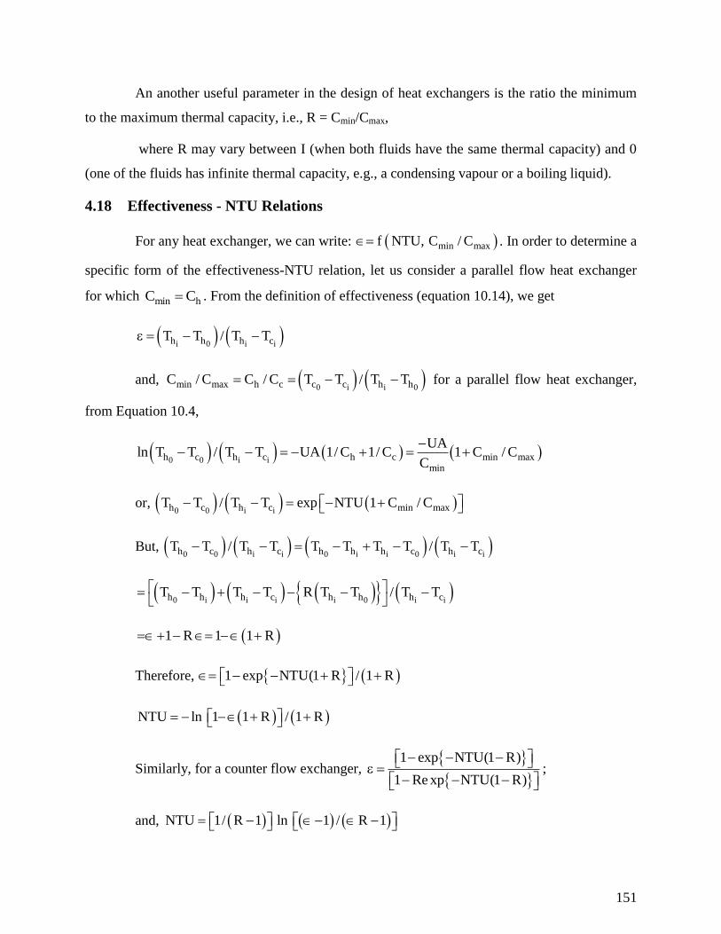
151

An another useful parameter in the design of heat exchangers is the ratio the minimum

to the maximum thermal capacity, i.e., R = Cmin/Cmax,

where R may vary between I (when both fluids have the same thermal capacity) and 0

(one of the fluids has infinite thermal capacity, e.g., a condensing vapour or a boiling liquid).

4.18 Effectiveness - NTU Relations

For any heat exchanger, we can write: min maxf NTU, C / C . In order to determine a

specific form of the effectiveness-NTU relation, let us consider a parallel flow heat exchanger

for which min hC C . From the definition of effectiveness (equation 10.14), we get

i 0 i ih h h cT T / T T

and, 0 i i 0min max h c c c h hC / C C / C T T / T T for a parallel flow heat exchanger,

from Equation 10.4,

0 0 i ih c h c h c min max

min

UAln T T / T T UA 1/ C 1/ C 1 C / C

C

or, 0 0 i ih c h c min maxT T / T T exp NTU 1 C / C

But, 0 0 i i 0 i i 0 i ih c h c h h h c h cT T / T T T T T T / T T

0 i i i i 0 i ih h h c h h h cT T T T R T T / T T

1 R 1 1 R

Therefore, 1 exp NTU(1 R / 1 R

NTU ln 1 1 R / 1 R

Similarly, for a counter flow exchanger,

1 exp NTU(1 R)

1 Re xp NTU(1 R)

;

and, NTU 1/ R 1 ln 1 / R 1

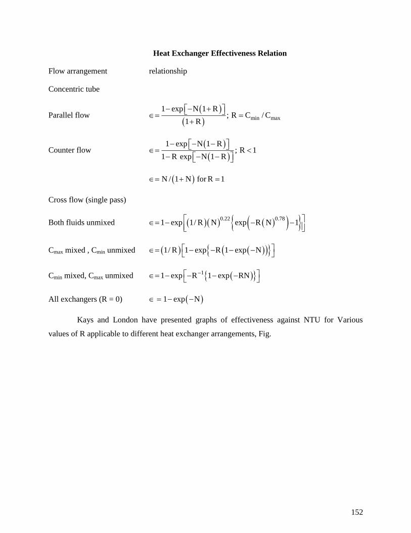
152

Heat Exchanger Effectiveness Relation

Flow arrangement relationship

Concentric tube

Parallel flow

min max

1 exp N 1 R; R C / C

1 R

Counter flow

1 exp N 1 R; R 1

1 R exp N 1 R

N / 1 N for R 1

Cross flow (single pass)

Both fluids unmixed 0.22 0.781 exp 1/ R N exp R N 1

Cmax mixed , Cmin unmixed 1/ R 1 exp R 1 exp N

Cmin mixed, Cmax unmixed 11 exp R 1 exp RN

All exchangers (R = 0) 1 exp N

Kays and London have presented graphs of effectiveness against NTU for Various

values of R applicable to different heat exchanger arrangements, Fig.

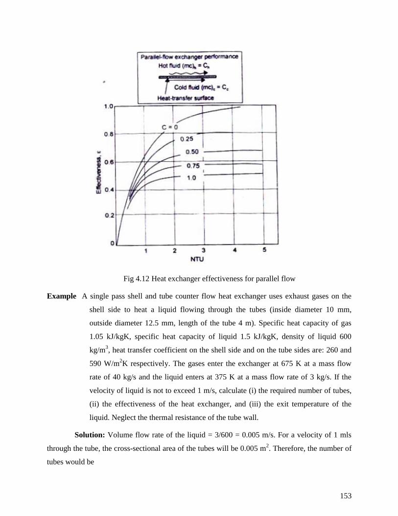
153

Fig 4.12 Heat exchanger effectiveness for parallel flow

Example A single pass shell and tube counter flow heat exchanger uses exhaust gases on the

shell side to heat a liquid flowing through the tubes (inside diameter 10 mm,

outside diameter 12.5 mm, length of the tube 4 m). Specific heat capacity of gas

1.05 kJ/kgK, specific heat capacity of liquid 1.5 kJ/kgK, density of liquid 600

kg/m3, heat transfer coefficient on the shell side and on the tube sides are: 260 and

590 W/m2K respectively. The gases enter the exchanger at 675 K at a mass flow

rate of 40 kg/s and the liquid enters at 375 K at a mass flow rate of 3 kg/s. If the

velocity of liquid is not to exceed 1 m/s, calculate (i) the required number of tubes,

(ii) the effectiveness of the heat exchanger, and (iii) the exit temperature of the

liquid. Neglect the thermal resistance of the tube wall.

Solution: Volume flow rate of the liquid = 3/600 = 0.005 m/s. For a velocity of 1 mls

through the tube, the cross-sectional area of the tubes will be 0.005 m2. Therefore, the number of

tubes would be

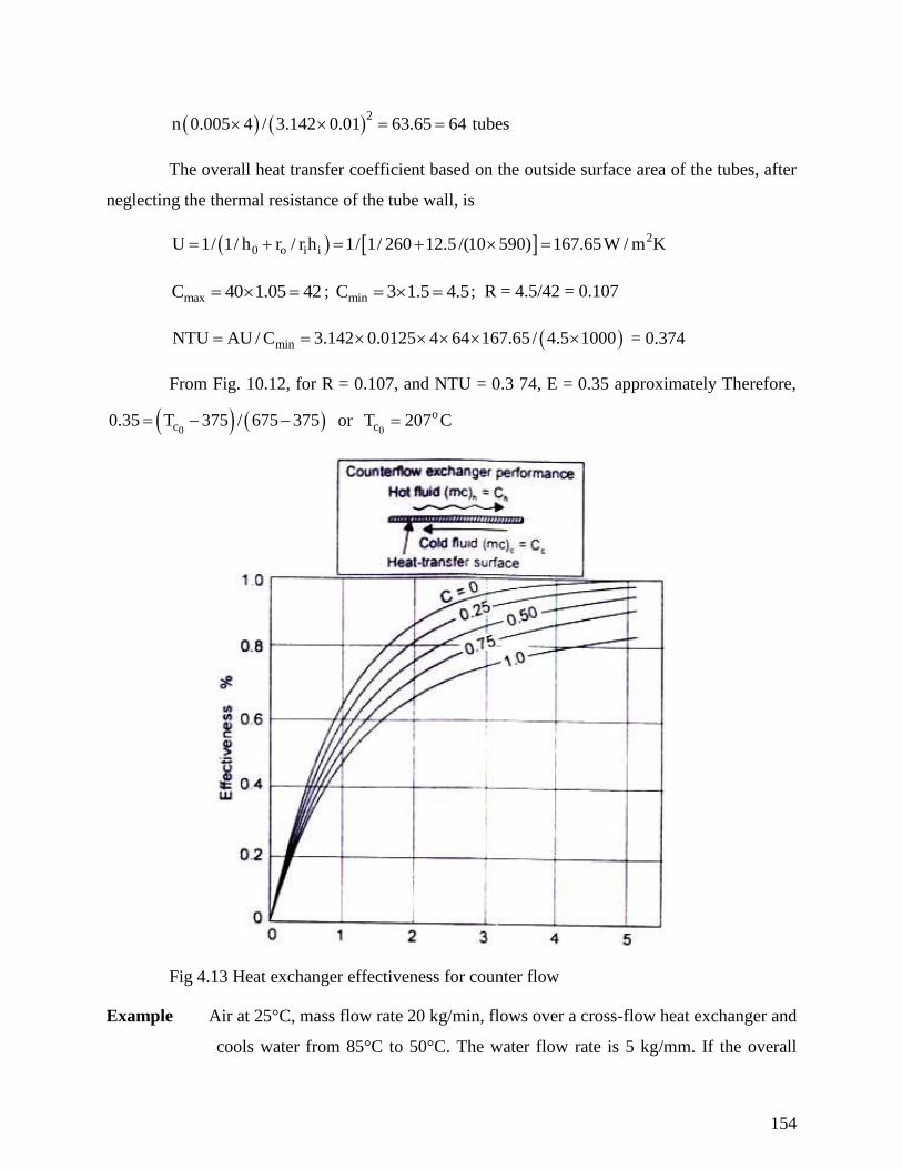
154

2

n 0.005 4 / 3.142 0.01 63.65 64 tubes

The overall heat transfer coefficient based on the outside surface area of the tubes, after

neglecting the thermal resistance of the tube wall, is

20 o i iU 1/ 1/ h r / r h 1/ 1/ 260 12.5 /(10 590) 167.65W / m K

maxC 40 1.05 42 ; minC 3 1.5 4.5 ; R = 4.5/42 = 0.107

minNTU AU / C 3.142 0.0125 4 64 167.65 / 4.5 1000 = 0.374

From Fig. 10.12, for R = 0.107, and NTU = 0.3 74, E = 0.35 approximately Therefore,

0c0.35 T 375 / 675 375 or

0

ocT 207 C

Fig 4.13 Heat exchanger effectiveness for counter flow

Example Air at 25°C, mass flow rate 20 kg/min, flows over a cross-flow heat exchanger and

cools water from 85°C to 50°C. The water flow rate is 5 kg/mm. If the overall

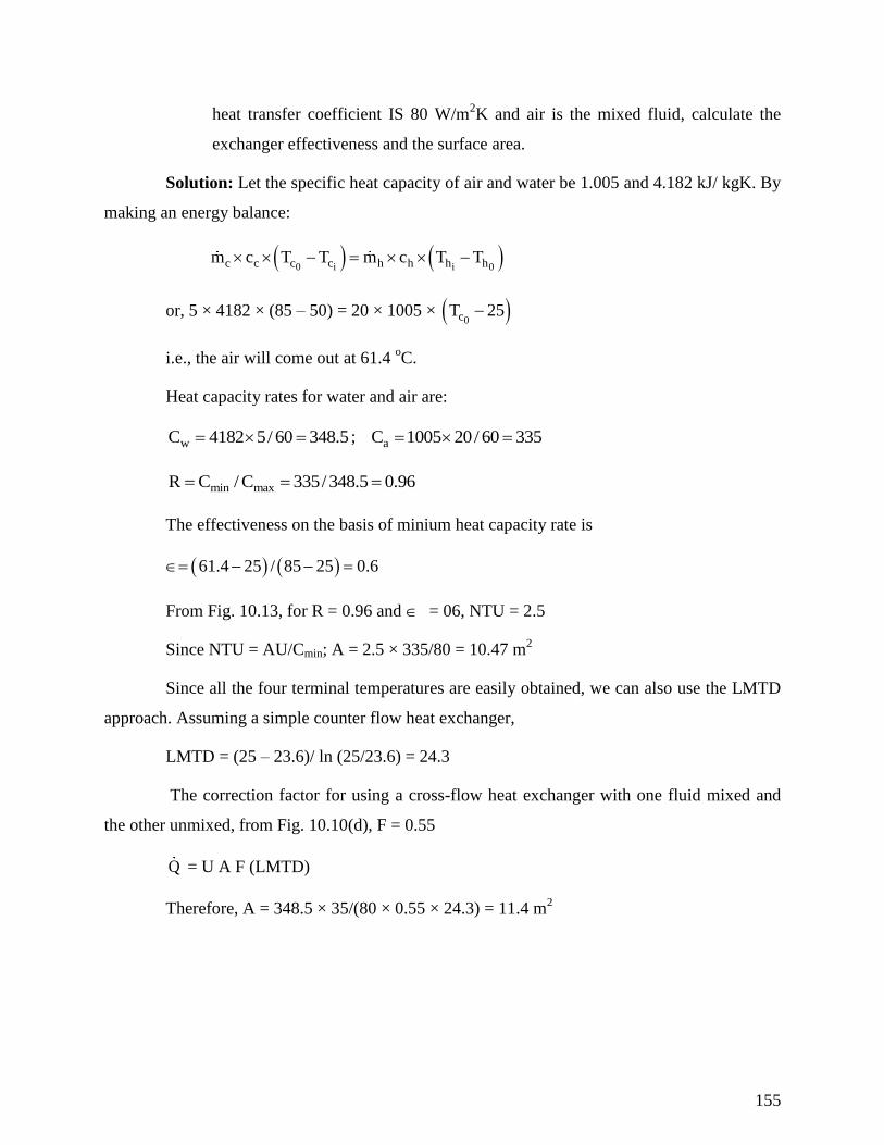
155

heat transfer coefficient IS 80 W/m2K and air is the mixed fluid, calculate the

exchanger effectiveness and the surface area.

Solution: Let the specific heat capacity of air and water be 1.005 and 4.182 kJ/ kgK. By

making an energy balance:

0 i i 0c c c c h h h hm c T T m c T T

or, 5 × 4182 × (85 – 50) = 20 × 1005 × 0cT 25

i.e., the air will come out at 61.4 oC.

Heat capacity rates for water and air are:

wC 4182 5/ 60 348.5 ; aC 1005 20/ 60 335

min maxR C / C 335/348.5 0.96

The effectiveness on the basis of minium heat capacity rate is

61.4 25 / 85 25 0.6

From Fig. 10.13, for R = 0.96 and = 06, NTU = 2.5

Since NTU = AU/Cmin; A = 2.5 × 335/80 = 10.47 m2

Since all the four terminal temperatures are easily obtained, we can also use the LMTD

approach. Assuming a simple counter flow heat exchanger,

LMTD = (25 – 23.6)/ ln (25/23.6) = 24.3

The correction factor for using a cross-flow heat exchanger with one fluid mixed and

the other unmixed, from Fig. 10.10(d), F = 0.55

Q = U A F (LMTD)

Therefore, A = 348.5 × 35/(80 × 0.55 × 24.3) = 11.4 m2

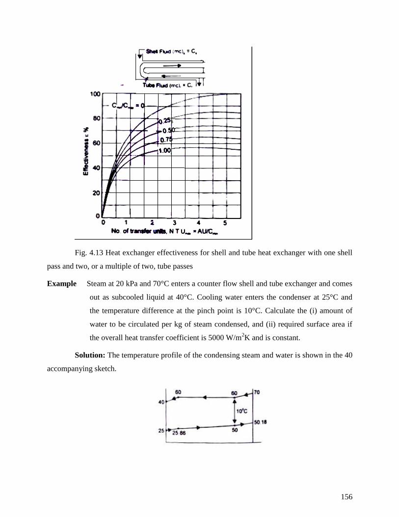
156

Fig. 4.13 Heat exchanger effectiveness for shell and tube heat exchanger with one shell

pass and two, or a multiple of two, tube passes

Example Steam at 20 kPa and 70°C enters a counter flow shell and tube exchanger and comes

out as subcooled liquid at 40°C. Cooling water enters the condenser at 25°C and

the temperature difference at the pinch point is 10°C. Calculate the (i) amount of

water to be circulated per kg of steam condensed, and (ii) required surface area if

the overall heat transfer coefficient is 5000 W/m2K and is constant.

Solution: The temperature profile of the condensing steam and water is shown in the 40

accompanying sketch.

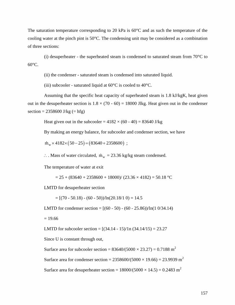
157

The saturation temperature corresponding to 20 kPa is 60°C and as such the temperature of the

cooling water at the pinch pint is 50°C. The condensing unit may be considered as a combination

of three sections:

(i) desuperheater - the superheated steam is condensed to saturated steam from 70°C to

60°C.

(ii) the condenser - saturated steam is condensed into saturated liquid.

(iii) subcooler - saturated liquid at 60°C is cooled to 40°C.

Assuming that the specific heat capacity of superheated steam is 1.8 kJ/kgK, heat given

out in the desuperheater section is 1.8 × (70 - 60) = 18000 Jlkg. Heat given out in the condenser

section = 2358600 J/kg (= hfg)

Heat given out in the subcooler = 4182 × (60 - 40) = 83640 J/kg

By making an energy balance, for subcooler and condenser section, we have

wm 4182 50 25 83640 2358600 ;

. Mass of water circulated, wm = 23.36 kg/kg steam condensed.

The temperature of water at exit

= 25 + (83640 + 2358600 + 18000)/ (23.36 × 4182) = 50.18 °C

LMTD for desuperheater section

= [(70 - 50.18) - (60 - 50))/ln(20.18/1 0) = 14.5

LMTD for condenser section = [(60 - 50) - (60 - 25.86))/ln(1 0/34.14)

= 19.66

LMTD for subcooler section = [(34.14 - 15)/1n (34.14/15) = 23.27

Since U is constant through out,

Surface area for subcooler section = 83640/(5000 × 23.27) = 0.7188 m2

Surface area for condenser section = 2358600/(5000 × 19.66) = 23.9939 m2

Surface area for desuperheater section = 18000/(5000 × 14.5) = 0.2483 m2

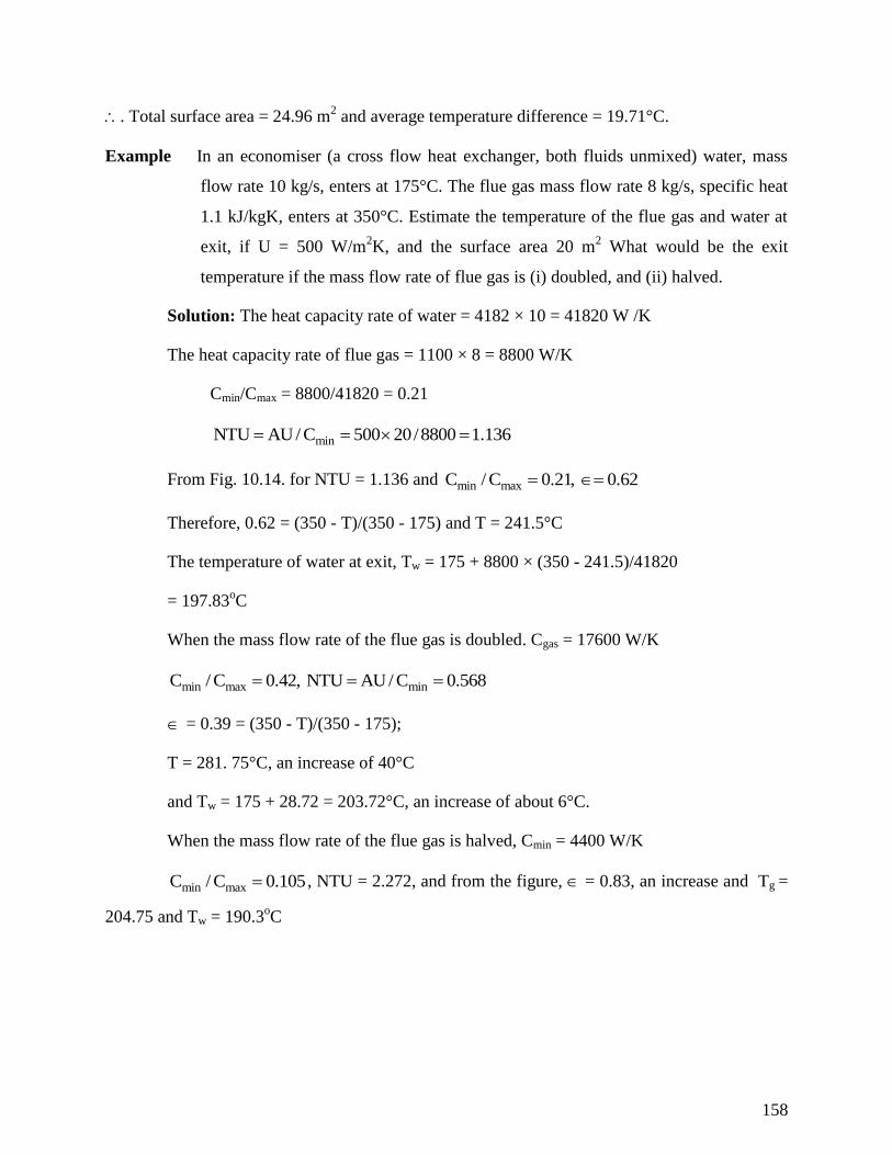
158

. Total surface area = 24.96 m2 and average temperature difference = 19.71°C.

Example In an economiser (a cross flow heat exchanger, both fluids unmixed) water, mass

flow rate 10 kg/s, enters at 175°C. The flue gas mass flow rate 8 kg/s, specific heat

1.1 kJ/kgK, enters at 350°C. Estimate the temperature of the flue gas and water at

exit, if U = 500 W/m2K, and the surface area 20 m

2 What would be the exit

temperature if the mass flow rate of flue gas is (i) doubled, and (ii) halved.

Solution: The heat capacity rate of water = 4182 × 10 = 41820 W /K

The heat capacity rate of flue gas = 1100 × 8 = 8800 W/K

Cmin/Cmax = 8800/41820 = 0.21

minNTU AU/ C 500 20/8800 1.136

From Fig. 10.14. for NTU = 1.136 and min maxC / C 0.21, 0.62

Therefore, 0.62 = (350 - T)/(350 - 175) and T = 241.5°C

The temperature of water at exit, Tw = 175 + 8800 × (350 - 241.5)/41820

= 197.83oC

When the mass flow rate of the flue gas is doubled. Cgas = 17600 W/K

min max minC / C 0.42, NTU AU/ C 0.568

= 0.39 = (350 - T)/(350 - 175);

T = 281. 75°C, an increase of 40°C

and Tw = 175 + 28.72 = 203.72°C, an increase of about 6°C.

When the mass flow rate of the flue gas is halved, Cmin = 4400 W/K

min maxC / C 0.105 , NTU = 2.272, and from the figure, = 0.83, an increase and Tg =

204.75 and Tw = 190.3oC

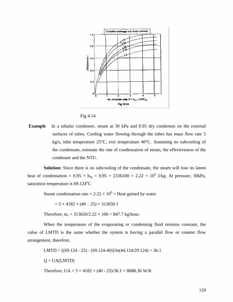
159

Fig 4.14

Example In a tubular condenser, steam at 30 kPa and 0.95 dry condenses on the external

surfaces of tubes. Cooling water flowing through the tubes has mass flow rate 5

kg/s, inlet temperature 25°C, exit temperature 40°C. Assuming no subcooling of

the condensate, estimate the rate of condensation of steam, the effectiveness of the

condenser and the NTU.

Solution: Since there is no subcooling of the condensate, the steam will lose its latent

heat of condensation = 0.95 × hfg = 0.95 × 2336100 = 2.22 × 106 J/kg. At pressure, 30kPa,

saturation temperature is 69.124oC

Steam condensation rate × 2.22 × 106 = Heat gained by water

= 5 × 4182 × (40 – 25) = 313650 J

Therefore, m, = 313650/2.22 × 106 = 847.7 kg/hour.

When the temperature of the evaporating or condensing fluid remains constant, the

value of LMTD is the same whether the system is having a parallel flow or counter flow

arrangement, therefore,

LMTD = [(69.124 - 25) - (69.124-40)]/ln(44.124/29.124) = 36.1

Q = UA(LMTD)

Therefore, UA = 5 × 4182 × (40 - 25)/36.1 = 8688.36 W/K

160

NTU = UA/Cmin = 8688.36/(5 × 4182) = 0.4155

Effectiveness= Actual temp. difference; Maximum possible temp. difference

= (40 - 25)/(69.124 - 25) = 34%.

Example A single shell 2 tube pass steam condenser IS used to cool steam entering at 50°C

and releasing 2000 MW of heat energy. The cooling water, mass flow rate 3 ×

104 kg/s, enters the condenser at 25°C. The condenser has 30,000 thin walled

tube of 30 mm diameter. If the overall heat transfer coefficient is 4000 Wim2K,

estimate the (I) rise m temperature of the cooling water, and (II) length of the

tube per pass.

Solution: By making an energy balance:

Heat released by steam = heat taken in by cooling water,

or, 2000 × 106 = 3 × 10

4 × 4182 × (

Since in a condenser, heat capacity rate of condensing steam is usually very large m

comparison with the heat capacity rate of cooling water, the effectiveness

0 i i ic c h cT T / T T 15.94 / 50 25 0.6376

And, for min maxC / C 0, 1 exp NTU

exp NTU 1.0 0.6376 0.3624

And, minNTU 1.015 AU / C 2 3.142 0.03 L 30000 4000 / 1.25 108

L = 5.546 m

4.19 Heat Exchanger Design-Important Factors

A comprehensive design of a heat exchanger involves the consideration of the thermal,

mechanical and manufacturing aspect. The choice of a particular design for a given duty depends

on either the selection of an existing design or the development of a new design. Before selecting

an existing design, the analysis of his performance must be made to see whether the required

performance would be obtained within acceptable limits.

161

In the development of a new design, the following factors are important:

(a) Fluid Temperature - the temperature of the two fluid streams are either specified for

a given inlet temperature, or the designer has to fix the outlet temperature based on flow rates

and heat transfer considerations. Once the terminal temperatures are defined, the effectiveness of

the heat exchanger would give an indication of the type of flow path-parallel or counter or cross-

flow.

(b) Flow Rates - The maximum velocity (without causing excessive pressure drops,

erosion, noise and vibration, etc.) in the case of liquids is restricted to 8 m1s and m case of gases

below 30 m/s. With this restriction, the flow rates of the two fluid streams lead to the selection of

flow passage cross-sectional area required for each of the two fluid steams.

(c) Tube Sizes and Layout - Tube sizes, thickness, lengths and pitches have strong

influence on heat transfer calculations and therefore, these are chosen with great care. The sizes

of tubes vary from 1/4" O.D. to 2" O.D.; the more commonly used sizes are: 5/8", 3/4" and 1"

O.D. The sizes have to be decided after making a compromise between higher heat transfer from

smaller tube sizes and the easy clean ability of larger tubes. The tube thickness will depend

pressure, corrosion and cost. Tube pitches are to be decided on the basis of heat transfer

calculations and difficulty in cleaning. Fig. 3.16 shows several arrangements for tubes in

bundles. The two standard types of pitches are the square and the triangle. the usual number 0 f

tube passes in a given shell ranges from one to eight. In multipass designs, even numbers of

passes are generally used because they are Simpler to design.

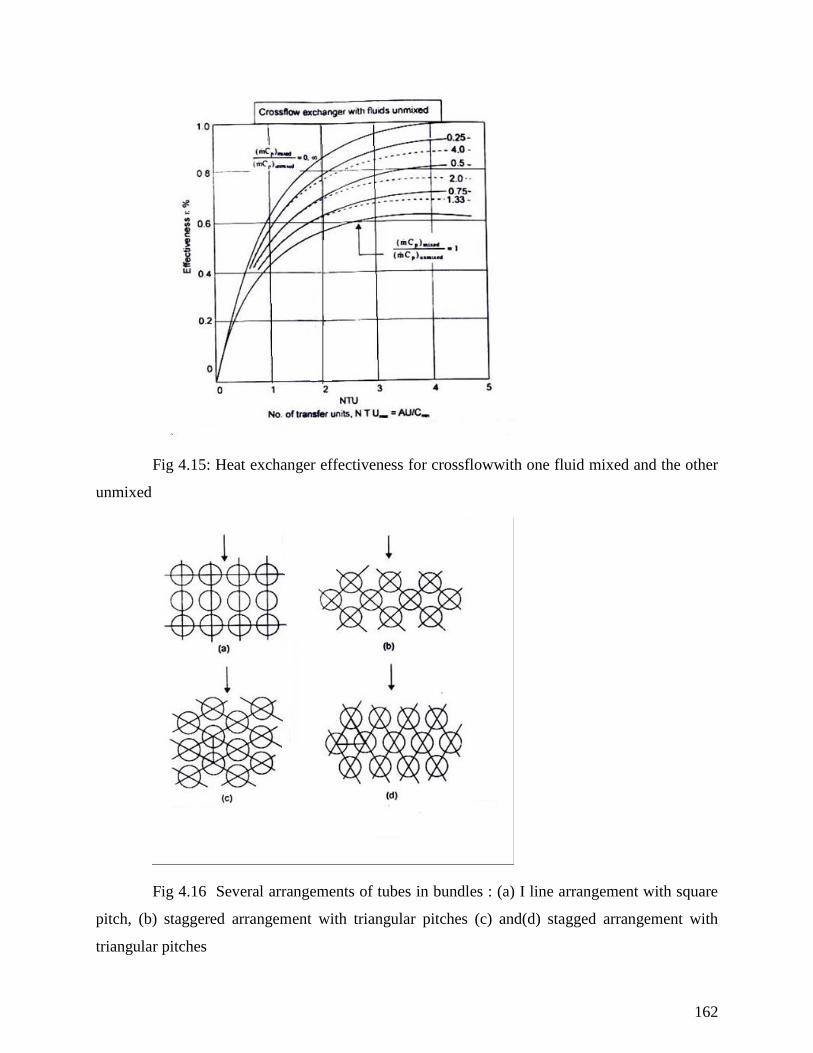
162

Fig 4.15: Heat exchanger effectiveness for crossflowwith one fluid mixed and the other

unmixed

Fig 4.16 Several arrangements of tubes in bundles : (a) I line arrangement with square

pitch, (b) staggered arrangement with triangular pitches (c) and(d) stagged arrangement with

triangular pitches

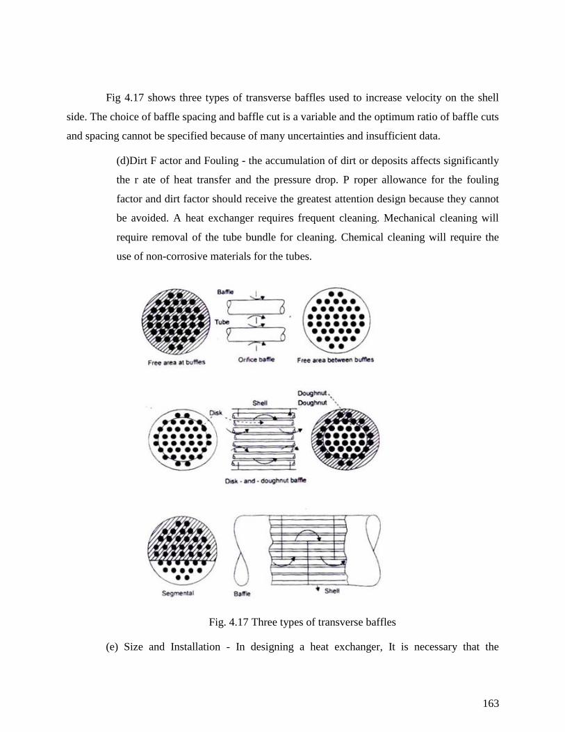
163

Fig 4.17 shows three types of transverse baffles used to increase velocity on the shell

side. The choice of baffle spacing and baffle cut is a variable and the optimum ratio of baffle cuts

and spacing cannot be specified because of many uncertainties and insufficient data.

(d)Dirt F actor and Fouling - the accumulation of dirt or deposits affects significantly

the r ate of heat transfer and the pressure drop. P roper allowance for the fouling

factor and dirt factor should receive the greatest attention design because they cannot

be avoided. A heat exchanger requires frequent cleaning. Mechanical cleaning will

require removal of the tube bundle for cleaning. Chemical cleaning will require the

use of non-corrosive materials for the tubes.

Fig. 4.17 Three types of transverse baffles

(e) Size and Installation - In designing a heat exchanger, It is necessary that the

164

constraints on length, height, width, volume and weight is known at the outset. Safety regulations

should also be kept in mind when handling fluids under pressure or toxic and explosive fluids.

(f) Mechanical Design Consideration - While designing, operating temperatures,

pressures, the differential thermal expansion and the accompanying thermal stresses require

attention.

And, above all, the cost of materials, manufacture and maintenance cannot be Ignored.

Example In a counter flow concentric tube heat exchanger cooling water, mass flow rate 0.2

kg/s, enters at 30°C through a tube inner diameter 25rnnl. The oil flowing

through the annulus, mass flow rate 0.1 kg/s, diameter 45 rum, has temperature at

inlet 100°C. Calculate the length of the tube if the oil comes out at 60°C. The

properties of oil and water are:

Oil: Cp – –2

Pa-s, k = 0.138 W/mK,

Water; Cp –6

Pa-s,

k = 0.625 W/mK, Pr = 4.85

Solution: By making an energy balance: Heat given out by oil = heat taken in by water.

0c0.1 2131 100 60 0.2 4187 T 30

0

ocT 40.2 C

LMTD = i 0 0 i i 0 0 0h c h c h c h cT T T T / ln T T / T T

o100 40.2 60 30 / ln 59.8 / 30 43.2 C

Since water is flowing through the tube,

6

4 0.2Re 4m / D

3.142 0.025 725 10

= 14050, a turbulent flow.

0.8 Pr

0.4, fluid being heated.

= 0.023 (14050)0.8

(4.85)0.4

= 90; ih = 90 × 0.625/0.025 = 2250 W/m2K

The oil is flowing through the annulus for which the hydraulic diameter is:

165

(0.045 - 0.025) = 0.02 m

2o iRe 4m / D D 4 0.1/ 3.142 0.07 3.25 10 56.0

laminar flow.

Assuming Uniform temperature along the Inner surface of the annulus and a perfectly

insulated outer surface.

Nu = 5.6, by interpolation (chapter 6)

ho = 5.6 × 0.138/0.02 = 38.6 W/m2K.

The overall heat transfer coefficient after neglecting the tube wall resistance,

U = 1/(1/2250 + 1/38.6) = 38 W/m2K

Q UA LMTD , where where A = iD L

L = (0.1 × 2131 × 40)/(38 × 3.142 × 0.025 × 43.2) = 66.1 m requires more than one

pass.

Example A double pipe heat exchanger has an effectiveness of 0.5 for the counter flow

arrangement and the thermal capacity of one fluid is twice that of the other fluid.

Calculate the effectiveness of the heat exchanger if the direction of flow of one of

the fluids is reversed with the same mass flow rates as before.

Solution: For a counter flow arrangement and R = 0.5, = 0.5

NTU 1/ R 1 ln R 1 2.0 ln 0.5 / 0.75 0.811

For parallel flow, = 1 exp NTU(1 R) / 1 R

1 exp 0.811 1.5 /1.5 0.469

Example Oil is cooled in a cooler from 65°C to 54°C by circulating water through the

cooler. The cooling load is 200 kW and water enters the cooler at 27°C. If the

overall heat transfer coefficient, based on the outer surface area of the tube is 740

W/m2K and the temperature rise of cooling water is 11°C, calculate the mass

flow rate of water, the effectiveness and the heat transfer area required for a

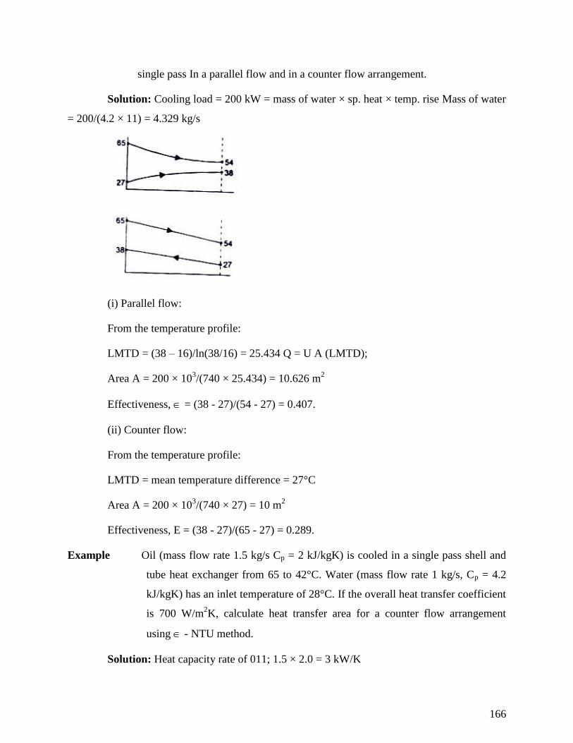
166

single pass In a parallel flow and in a counter flow arrangement.

Solution: Cooling load = 200 kW = mass of water × sp. heat × temp. rise Mass of water

= 200/(4.2 × 11) = 4.329 kg/s

(i) Parallel flow:

From the temperature profile:

LMTD = (38 – 16)/ln(38/16) = 25.434 Q = U A (LMTD);

Area A = 200 × 103/(740 × 25.434) = 10.626 m

2

Effectiveness, = (38 - 27)/(54 - 27) = 0.407.

(ii) Counter flow:

From the temperature profile:

LMTD = mean temperature difference = 27°C

Area A = 200 × 103/(740 × 27) = 10 m

2

Effectiveness, E = (38 - 27)/(65 - 27) = 0.289.

Example Oil (mass flow rate 1.5 kg/s Cp = 2 kJ/kgK) is cooled in a single pass shell and

tube heat exchanger from 65 to 42°C. Water (mass flow rate 1 kg/s, Cp = 4.2

kJ/kgK) has an inlet temperature of 28°C. If the overall heat transfer coefficient

is 700 W/m2K, calculate heat transfer area for a counter flow arrangement

using - NTU method.

Solution: Heat capacity rate of 011; 1.5 × 2.0 = 3 kW/K

167

Heat capacity rate of water = 1 × 4.2; 4.2 kW/K

minC 3.0 kW/ K and min maxR C / C 3/ 4.2 0.714

For a counter flow arrangement, NTU 1/ R 1 ln 1 / R 1

Effectiveness, 65 42 / 65 28 0.6216

and NTU = 1.346 = minAU/ C ; A = 1.346 × 3000 / 700 = 5.77 m2

By making an energy balance, we can compute the water temperature at outlet.

or 3.0 × (65 - 42); 4.2 × (T - 28), T; 44.428

LMTD for a counter flow arrangement:

LMTD; (20.572 - 14)/ln (20.572/14) = 17.076

Area, A = 3 2Q / U LMTD 3 10 65 42 / 700 17.076 5.77 m

Example A fluid (mass flow rate 1000 kg/min, sp. heat capacity 3.6 kJ/kgK) enters a heat

exchanger at 700 C. Another fluid (mass flow rate 1200 kg/mm, sp. heal capacity

4.2 kJ/kgK) enters al 100 C. If the overall heat transfer coefficient is 420 W/m2K

and the surface area is 100m2, calculate the outlet temperatures of both fluids for

both counter flow and parallel flow arrangements.

Solution: Heat capacity rate for the hot fluid

3 31000 3.6 10 60 60 10 W/ K

Heat capacity rate for the cold fluid = 1200 × 4.2 × 103/60 = 84 × 10

3 W/K

R = Cmin/Cmax = 60/84; 0.714, NTU = U A/Cmin = 420 × 100/60000 = 0.7

(i) For counter flow heat exchanger:

1 exp N 1 R / 1 Re xp N 1 R

1 exp 0.7 1 0.714 /1 1 0.714 exp 0.7 1 0.714 0.4367

Since heat capacity rate of the hot fluid IS lower,

168

0h700 T / 700 100

and 0

ohT 700 0.4367 600 438 C

By making an energy balance, 0

3 3c60 10 700 438 84 10 T 100

or, 0

ocT 60 262 / 84 100 87.14 C

(ii) For parallel flow heat exchanger

1 exp N 1 R / 1 R 1 exp 0.7 1 0.714 / 1.714

0.4077 , a lower value

and i 0 i 0 0 0h h h c h cT T / T T 0.4077 700 T / 700 T

By making an energy balance: 0 0

3 3h c60 10 700 T 84 10 T 100

or, 0 0c h700 T 700 T / 0.4077

and 0 0c c84 T 100 / 60 1.4T 140

Therefore, 0

ocT 237.5 C

and 0

ohT 511.4 C

Example Steam enters the surface condenser at 100°C and water enters at 25°C with a

temperature rise of 25°C. Calculate the effectiveness and the NTU for the

condenser. If the water temperature at inlet changes to 35 C, estimate the

temperature rise for water.

Solution: Effectiveness, = 25/(100 25) = 0.33

For R = 0, = 1 - exp(- N)

or, N = -ln(1 - ) = 0.405

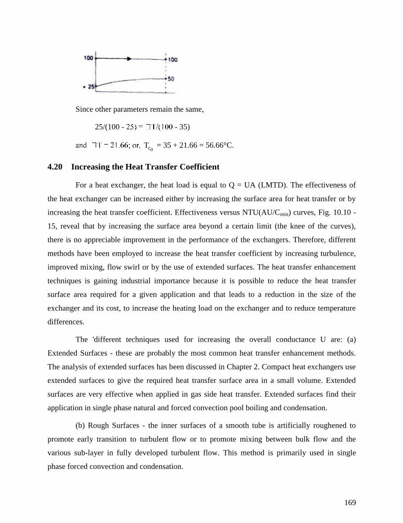
169

Since other parameters remain the same,

25/(100 - - 35)

0cT = 35 + 21.66 = 56.66°C.

4.20 Increasing the Heat Transfer Coefficient

For a heat exchanger, the heat load is equal to Q = UA (LMTD). The effectiveness of

the heat exchanger can be increased either by increasing the surface area for heat transfer or by

increasing the heat transfer coefficient. Effectiveness versus NTU(AU/Cmin) curves, Fig. 10.10 -

15, reveal that by increasing the surface area beyond a certain limit (the knee of the curves),

there is no appreciable improvement in the performance of the exchangers. Therefore, different

methods have been employed to increase the heat transfer coefficient by increasing turbulence,

improved mixing, flow swirl or by the use of extended surfaces. The heat transfer enhancement

techniques is gaining industrial importance because it is possible to reduce the heat transfer

surface area required for a given application and that leads to a reduction in the size of the

exchanger and its cost, to increase the heating load on the exchanger and to reduce temperature

differences.

The 'different techniques used for increasing the overall conductance U are: (a)

Extended Surfaces - these are probably the most common heat transfer enhancement methods.

The analysis of extended surfaces has been discussed in Chapter 2. Compact heat exchangers use

extended surfaces to give the required heat transfer surface area in a small volume. Extended

surfaces are very effective when applied in gas side heat transfer. Extended surfaces find their

application in single phase natural and forced convection pool boiling and condensation.

(b) Rough Surfaces - the inner surfaces of a smooth tube is artificially roughened to

promote early transition to turbulent flow or to promote mixing between bulk flow and the

various sub-layer in fully developed turbulent flow. This method is primarily used in single

phase forced convection and condensation.

170

(c) Swirl Flow Devices - twisted strips are inserted into the flow channel to impart a

rotational motion about an axis parallel to the direction of bulk flow. The heat transfer coefficient

increases due to increased flow velocity, secondary flows generated by swirl, or increased flow

path length in the flow channel. This technique is used in flow boiling and single phase forced

flow.

(d) Treated Surfaces - these are used mainly in pool boiling and condensation.

Treated surfaces promote nucleate boiling by providing bubble nucleation sites. The rate

of condensation increases by promoting the formation of droplets, instead of a liquid film on the

condensing surface. This can be accomplished by coating the surface with a material that makes

the surface non-wetting.

All of these techniques lead to an increase in pumping work (increased frictional

losses) and any practical application requires the economic benefit of increased overall

conductance. That is, a complete analysis should be made to determine the increased first cost

because of these techniques, increased heat exchanger heat transfer performance, the effect on

operating costs (especially a substantial increase in pumping power) and maintenance costs.

4.21 Fin Efficiency and Fin Effectiveness

Fins or extended surfaces increase the heat transfer area and consequently, the amount

of heat transfer is increased. The temperature at the root or base of the fin is the highest and the

temperature along the length of the fm goes on decreasing Thus, the fin would dissipate the

maximum amount of heat energy if the temperature all along the length remains equal to the

temperature at the root. Thus, the fin efficiency is defined as:

fin = (actual heat transferred) / (heat which would be transferred if the entire fin area

were at the root temperature)

In some cases, the performance of the extended surfaces is evaluated by comparing the

heat transferred with the fin to the heat transferred without the fin. This ratio is called 'fin

effectiveness' E and it should be greater than 1, if the rate of heat transfer has to be increased

with the use of fins.

For a very long fin, effectiveness E = Q with fin / Q without fin

171

= (hpkA)1/ 2

0 /hA 0 = (kp/hA)1/2

And fin = (hpkA) 1/ 2

0 (hpL 0 ) = (hpkA)1/2

/ (hpL)

1/ 2

1/ 2fin

kp / hAE pL Surface area of finhpL

A Cross-sectional area of the finhpkA

i.e., effectiveness increases by increasing the length of the fin but it will decrease the fin

efficiency.

Expressions for Fin Efficiency for Fins of Uniform Cross-section

1. Very long fins: 1/ 2

0 0hpkA T T / hpL T T 1/ mL

2 For fins having insulated tips:

1/ 2

0

0

hpkA T T tan h mL tan h (mL)

hpL T T mL

Example The total efficiency for a finned surface may be defined as the ratio of the

total heat transfer of the combined area of the surface and fins to the heat which would be

transferred if this total area were maintained at the root temperature T0 . Show that this efficiency

can be calculated from

t = 1 - Af / A(1 - t ) where t = total effltiency, Af = surface area of all fins, A = total

heat transfer area, f = fin efficiency

Solution: Fin efficiency,

f = Actual heat transfered

Heat that would be transferred if the en tire fin were at the root temperature

or, f = f 0

Actual heat transfer

hA T T

Actual heat transfer from finned surface = f f 0hA (T T )

Actual heat transfer from un finned surface which are at the root temperature: h(A-Af)

172

0(T T )

Actual total heat transfer = h(A -Af ) 0(T T ) + f f 0hA (T T )

By the definition of total efficiency,

t f 0 f f 0 0h A A T T hA T T / hA T T

= f f fA A hA

A

= f f f1 A / A A / A

= f f1 A / A 1 .

4.23. Extended Surfaces do not always Increase the Heat Transfer Rate

The installation of fins on a heat transferring surface increases the heat transfer area but

it is not necessary that the rate of heat transfer would increase. For long fins, the rate of heat loss

from the fin is given by (hpkA)1/ 2

0 = kA(hp/kA) 1/ 2

0 = kAm 0 . When h/ mk = 1, Q = hA 0

which is equal to the heat loss from the primary surface with no extended surface. Thus, when h

= mk, an extended surface will not increase the heat transfer rate from the primary surface

whatever be the length of the extended surface.

For h/mk > 1, Q < hA 0 and hence adding a secondary surface reduces the heat

transfer, and the added surface will act as an insulation. For h/mk < 1, Q > hA 0 , and the

extended surface will increase the heat transfer, Fig. 2.3l. Further, h/mk=(h2.kA/k

2hp)

1/2 =

(hA/kP)1/2

, i.e. when h/mk < 1, the heat transfer would be more effective when h/k is low for a

given geometry.

4.24 An Expression for Temperature Distribution for an Annular Fin of Uniform

Thickness

In order to increase the rate of heat transfer from cylinders of air-cooled engines and in

certain type of heat exchangers, annular fins of uniform cross-section are employed. Fig. 2.32

shows such a fin with its nomenclature.

In the analysis of such fins, it is assumed that:

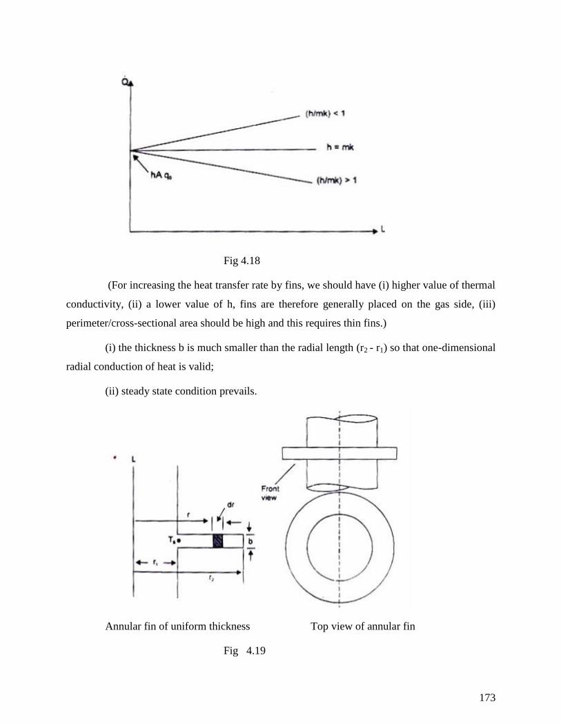
173

Fig 4.18

(For increasing the heat transfer rate by fins, we should have (i) higher value of thermal

conductivity, (ii) a lower value of h, fins are therefore generally placed on the gas side, (iii)

perimeter/cross-sectional area should be high and this requires thin fins.)

(i) the thickness b is much smaller than the radial length (r2 - r1) so that one-dimensional

radial conduction of heat is valid;

(ii) steady state condition prevails.

Annular fin of uniform thickness Top view of annular fin

Fig 4.19

174

We choose an annular element of radius r and radial thickness dr. The cross-sectional

area for radial heat conduction at radius r is 2 rb and at radius r + dr is 2 (r + dr)b. The surface

area for convective heat transfer for the annulus is 2(2 r.dr). Thus, by making an energy

balance,

2

2

dT dT d Tk2 rb k2 r dr b dr h 4 r.dr T T

dr dr dr

or, d2T / dr

2 +(1 /r)dT / dr- 2h/kb(T - T ) = 0

Let, = (T - T ) the above equation reduces to

d2 / dr

2 +(l/r) d /dr -(2h kb) = 0

The equation is recognised as Bessel's equation of zero order and the solution is = C1

I0 (nr)+C2 K0 (nr), where n=(2h/kb)1/2

,I0 is the modified Bessel function, 1st kind and K0 is the

modified Bessel function, 2nd kind, zero order, The constants C1 and C2 are evaluated by

applying the two boundary conditions:

at r = rl, T = Ts and = Ts - T

at r = r 2, dT / dr = 0 because b < < (r 2 - rl )

By applying the boundary conditions, the temperature distribution is given by

0 1 2 0 1 2

0 0 1 1 2 0 1 1 2

I nr K (nr ) K nr I nr

I nr K (nr ) K nr I nr

(3.16)

I1 (nr) and K1 (nr) are Bessel functions or order one.

And the rate of heat transfer is given by:

1 1 1 2 1 1 1 2

0 10 1 1 2 0 1 1 2

K nr I (nr ) I nr K nrQ 2 knb r

K nr I (nr ) I nr K nr

(3.17)

Table 2.1 gives selected values of the Modified Bessel Functions of the First and

Second kinds, order Zero and One. (The details of solution can be obtained from: C.R. Wylie, Jr:

Advanced Engineering Mathematics, McGraw-Hill Book Company, New York.)

The efficiency of circumferential fins is also obtained from curves for efficiencies

175

3 1

2 2

2 1 2 1

b 2halong Y-axis r r r r

2 Kb

for different values of 2 1

br / r

2

.

176

SCHOOL OF MECHANICAL

DEPARTMENT OF MECHANICAL

UNIT – V – Heat and Mass Transfer – SMEA1504

177

UNIT:5 MASS TRANSFER

Definition:

Transfer of mass as a result of particle concentration difference in a mixture.

Air is a mixture of various gases. Whenever we have a multi component system with a

concentration gradient, one constituent of the mixture gets transported from the region of

higher concentration to the region of lower concentration till the concentration gradient

reduces to zero. This phenomenon of the transport of mass as a result of concentration

gradient is called 'Mass Transfer'.

Difference of Heat transfer and Mass Transfer

Heat Transfer Mass transfer

Temperature Gradient a Concentration Gradient

Occurs from higher temperature to

lower temperature

b Occurs from higher Concentration to lower

concentration

Modes of Mass Transfer

There are basically three modes of mass transfer:

i. Diffusion mass Transfer

occurs due to concentration difference

Transport of matter in microscopic level

Occurs between higher concentration and lower concentration

Eg. Osmosis, Reverse osmosis, Leakage of air from automobile and leakage of LPG from tanks

ii. Convective Mass Transfer

occurs due to concentration difference and velocity

Concentration of particles at its surface differs from its concentration in a gas moving

over the surface

Eg. Drying of clothes, evaporization of water from swimming pool.

iii. Phase change Mass Transfer

occurs due to simultaneous effect of convection and diffusion mass transfer

Eg. Burnt gases from chimney rise by convection and then mixes with air by diffusion

178

Problem 1:

The composition of dry atmospheric air on a molar basis is 78.1% N2, 20.9% O

2, and 1% Ar.

Neglecting other constituents, Assuming atmospheric pressure 1bar and temperature 27⁰C.

Find the mass fractions of the constituents of air.

179

Fick’s law of diffusion

The molar flux (Rate of Mass transfer) is directly proportional to concentration difference

and inversely proportional to separation.

where, Dab

= Diffusion coefficient or Diffusivity (m2

/sec)

And Ca = concentration or molecules per unit volume of the particles

= Solubility x Pressure

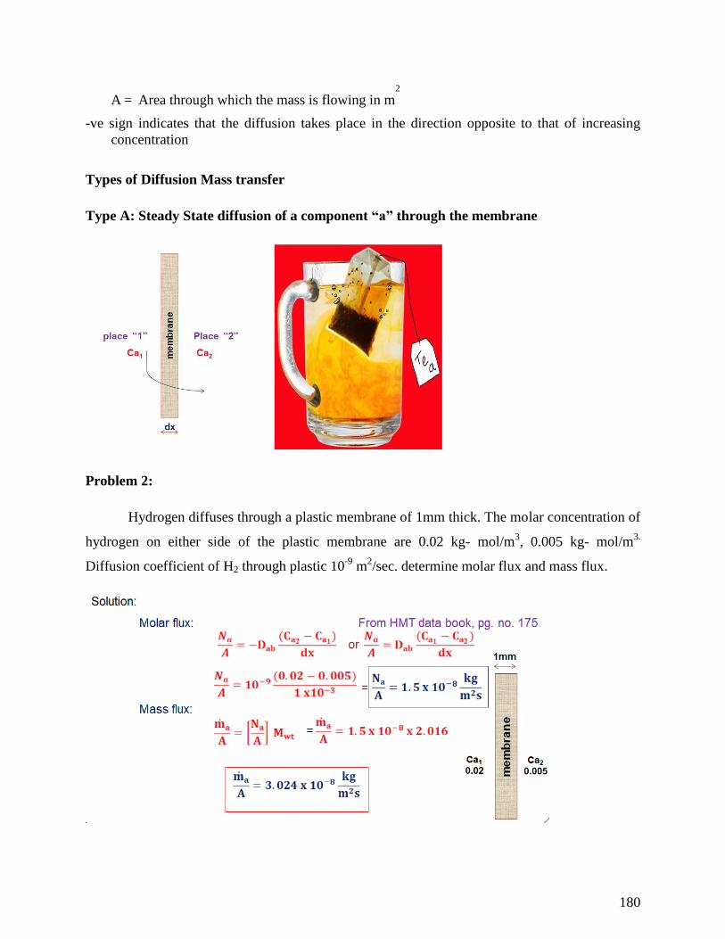
180

A = Area through which the mass is flowing in m2

-ve sign indicates that the diffusion takes place in the direction opposite to that of increasing

concentration

Types of Diffusion Mass transfer

Type A: Steady State diffusion of a component “a” through the membrane

Problem 2:

Hydrogen diffuses through a plastic membrane of 1mm thick. The molar concentration of

hydrogen on either side of the plastic membrane are 0.02 kg- mol/m3, 0.005 kg- mol/m

3.

Diffusion coefficient of H2 through plastic 10-9

m2/sec. determine molar flux and mass flux.

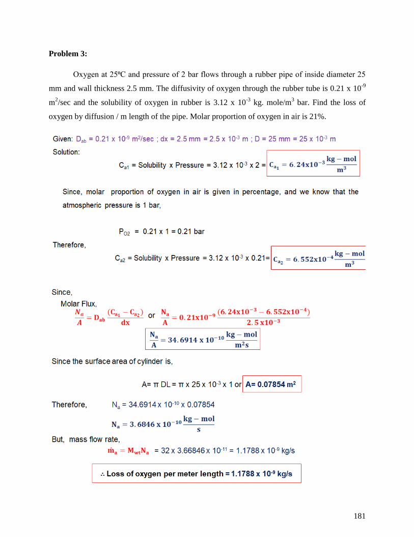
181

Problem 3:

Oxygen at 25⁰C and pressure of 2 bar flows through a rubber pipe of inside diameter 25

mm and wall thickness 2.5 mm. The diffusivity of oxygen through the rubber tube is 0.21 x 10-9

m2/sec and the solubility of oxygen in rubber is 3.12 x 10

-3 kg. mole/m

3 bar. Find the loss of

oxygen by diffusion / m length of the pipe. Molar proportion of oxygen in air is 21%.

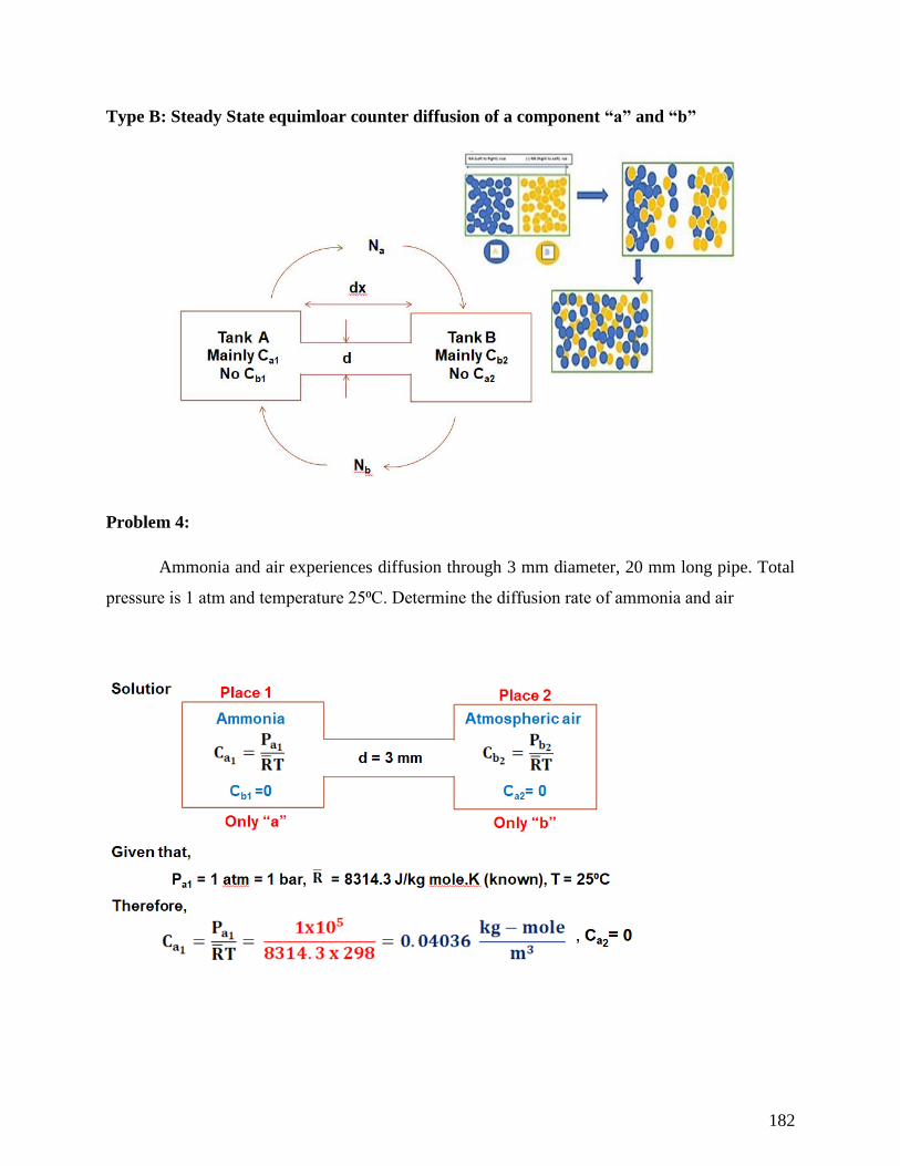
182

Type B: Steady State equimloar counter diffusion of a component “a” and “b”

Problem 4:

Ammonia and air experiences diffusion through 3 mm diameter, 20 mm long pipe. Total

pressure is 1 atm and temperature 25⁰C. Determine the diffusion rate of ammonia and air

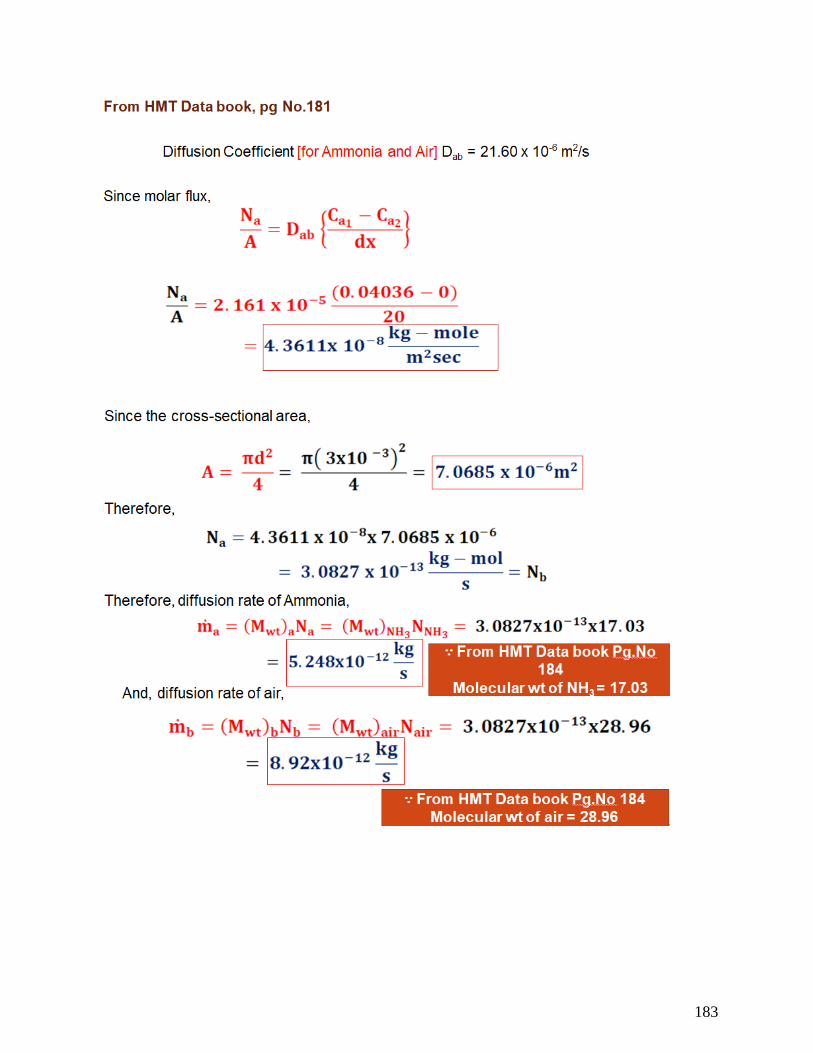
183

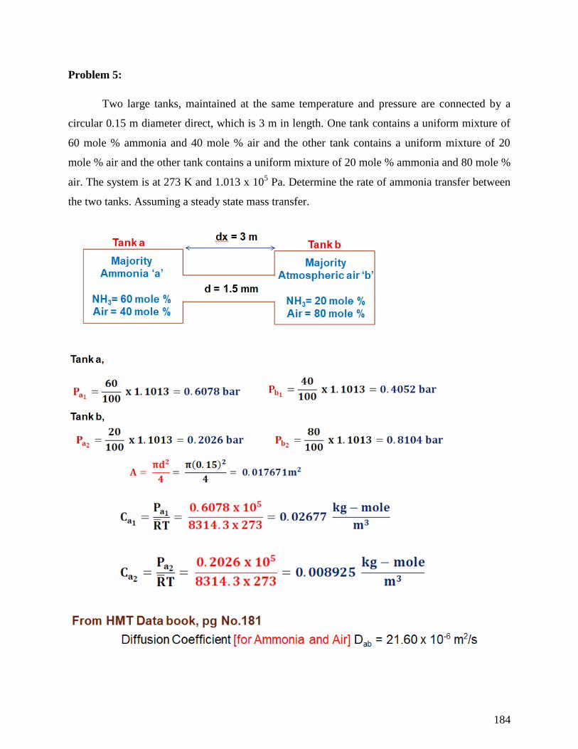
184

Problem 5:

Two large tanks, maintained at the same temperature and pressure are connected by a

circular 0.15 m diameter direct, which is 3 m in length. One tank contains a uniform mixture of

60 mole % ammonia and 40 mole % air and the other tank contains a uniform mixture of 20

mole % air and the other tank contains a uniform mixture of 20 mole % ammonia and 80 mole %

air. The system is at 273 K and 1.013 x 105 Pa. Determine the rate of ammonia transfer between

the two tanks. Assuming a steady state mass transfer.

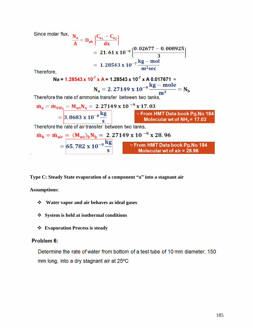
185

Type C: Steady State evaporation of a component “a” into a stagnant air

Assumptions:

Water vapor and air behaves as ideal gases

System is held at isothermal conditions

Evaporation Process is steady

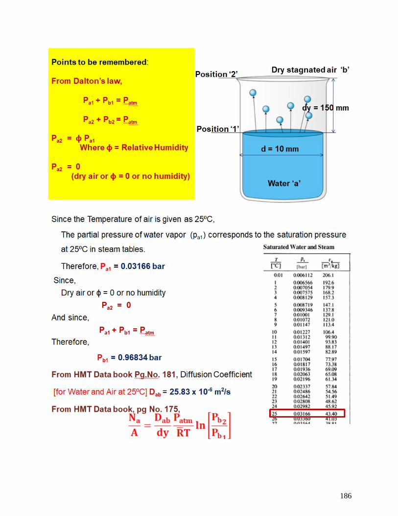
186

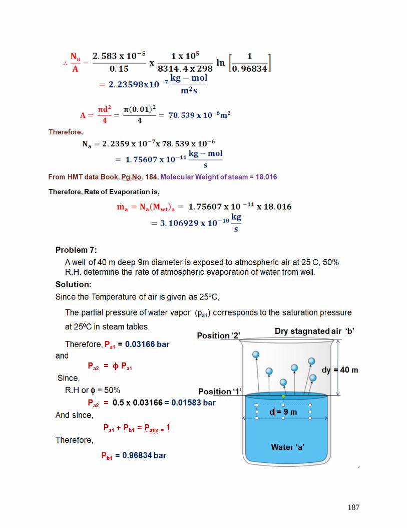
187

188

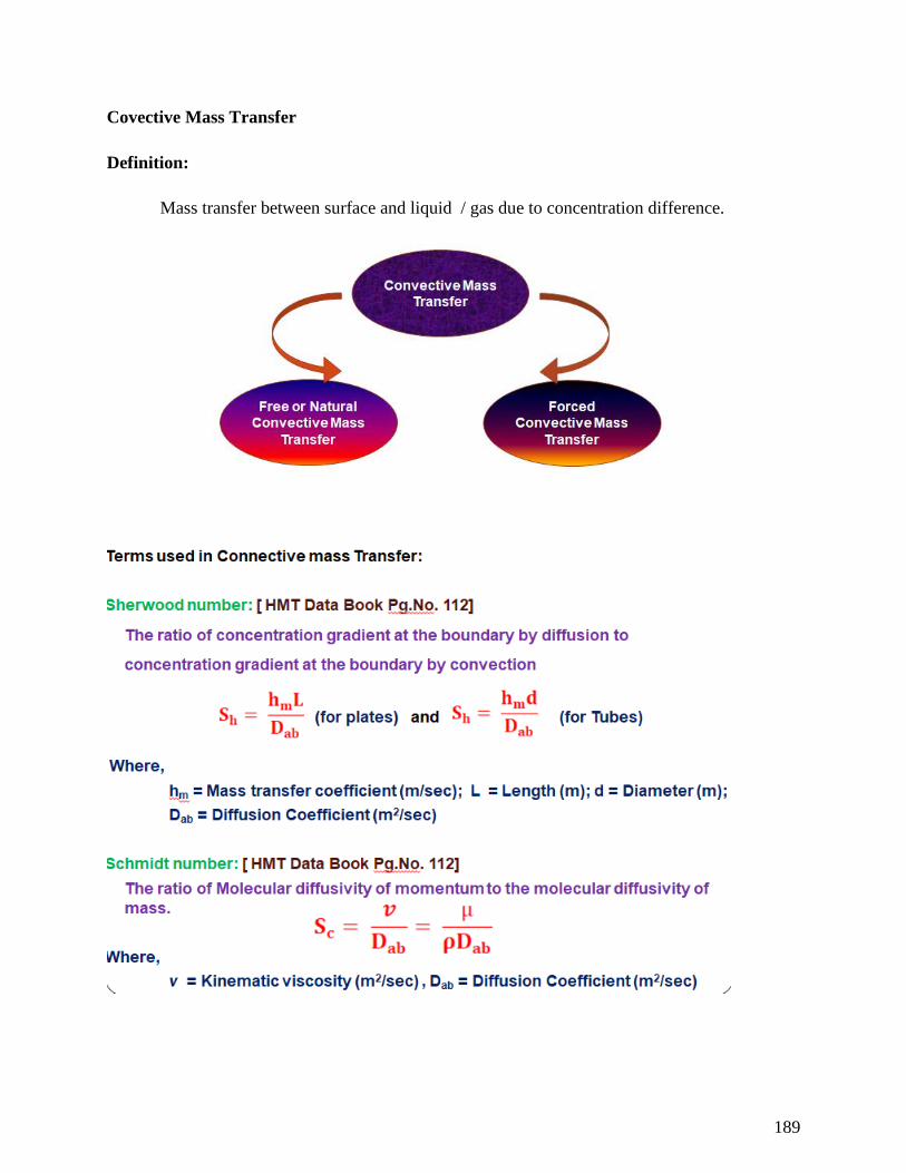
189

Covective Mass Transfer

Definition:

Mass transfer between surface and liquid / gas due to concentration difference.

190

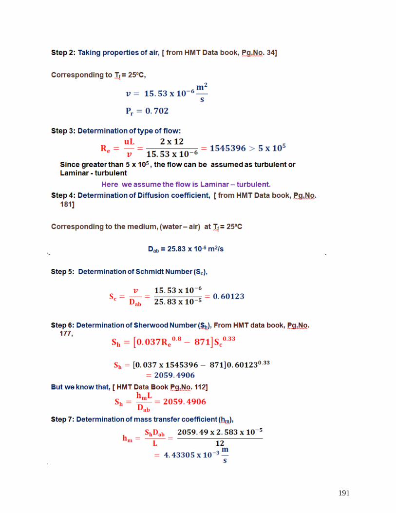
191

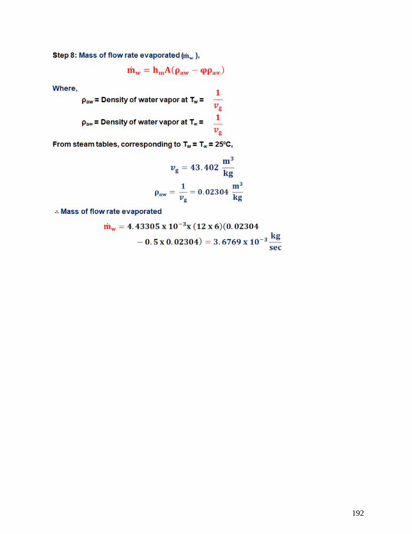
192