TH

E

U N I V E RS

IT

Y

OF

ED I N B U

RG

H

School of Informatics, University of Edinburgh

Institute for Adaptive and Neural Computation

Temporal Hidden Hopfield Models

by

Felix Agakov, David Barber

Informatics Research Report EDI-INF-RR-0156

School of Informatics November 2002http://www.informatics.ed.ac.uk/

Temporal Hidden Hopfield Models

Felix Agakov, David Barber

Informatics Research Report EDI-INF-RR-0156

SCHOOLof INFORMATICSInstitute for Adaptive and Neural Computation

November 2002

Abstract :Many popular probabilistic models for temporal sequences assume simple hidden dynamics or low dimensionality

of discrete variables. For higher dimensional discrete hidden variables, recourse is often made to approximate meanfield theories, which to date have been applied to models with only simple hidden unit dynamics. We consider a classof models in which the discrete hidden space is defined by parallel dynamics of densely connected high-dimensionalstochastic Hopfield networks. For these Hidden Hopfield Models (HHMs), mean field methods are derived for learningdiscrete and continuous temporal sequences. We discuss applications of HHMs to classification and reconstructionof non-stationary time series. We also demonstrate a few problems (learning of incomplete binary sequences andreconstruction of 3D occupancy graphs) where distributed discrete hidden space representation may be useful. Weshow that while these problems cannot be easily solved by other dynamic belief networks, they are efficiently addressedby HHMs.

Keywords : Dynamic belief networks, Hidden Markov Models, Hopfield networks, variational learning, missing data,temporal sequences.

Copyright c 2002 by The University of Edinburgh. All Rights Reserved

The authors and the University of Edinburgh retain the right to reproduce and publish this paper for non-commercialpurposes.

Permission is granted for this report to be reproduced by others for non-commercial purposes as long as this copy-right notice is reprinted in full in any reproduction. Applications to make other use of the material should be addressedin the first instance to Copyright Permissions, Division of Informatics, The University of Edinburgh, 80 South Bridge,Edinburgh EH1 1HN, Scotland.

Temporal Hidden Hopfield Models

Felix V. Agakov and David Barber

Division of Informatics, University of Edinburgh, Edinburgh EH1 2QL, UK

felixa@anc.ed.ac.uk, dbarber@anc.ed.ac.ukhttp://anc.ed.ac.uk

November 4, 2002

Abstract

Many popular probabilistic models for temporal sequences assume simple hidden dy-namics or low-dimensionality of discrete variables. For higher dimensional discrete hiddenvariables, recourse is often made to approximate mean field theories, which to date havebeen applied to models with only simple hidden unit dynamics. We consider a class of mod-els in which the discrete hidden space is defined by parallel dynamics of densely connectedhigh-dimensional stochastic Hopfield networks. For these Hidden Hopfield Models (HHMs),mean field methods are derived for learning discrete and continuous temporal sequences.We discuss applications of HHMs to classification and reconstruction of non-stationary timeseries. We also demonstrate a few problems (learning of incomplete binary sequences andreconstruction of 3D occupancy graphs) where distributed discrete hidden space represen-tation may be useful. We show that while these problems cannot be easily solved by otherdynamic belief networks, they are efficiently addressed by HHMs.

1 Markovian Dynamics for Temporal Sequences

Dynamic Bayesian networks are popular tools for modeling temporally correlated patterns. In-cluded in this class of models are Hidden Markov Models (HMMs), auto-regressive HMMs (seee.g. Rabiner (1989)), and Factorial HMMs (Ghahramani and Jordan, 1995). These models arespecial cases of a generalized Markov chain

p({h}, {v}) = p(h(0))p(v(0))

T−1∏

t=0

p(h(t+1)|h(t), v(t))p(v(t+1)|h(t), v(t)), (1)

where {h} = {h(0), . . . , h(T )} and {v} = {v(0), . . . , v(T )} are hidden and visible variables [seeFigure 1 (a)–(c)].

A general procedure for learning the model parameters Θ by maximum likelihood trainingis the EM algorithm, which optimizes a lower bound on the likelihood

Φ({v}; q,Θ) = 〈log p({h}, {v}) + log q({h}|{v})〉q({h}|{v}) (2)

with respect to the parameters [the M-step] and an auxiliary distribution q({h}|{v}) [the E-step]. The bound on the likelihood L is exact if and only if q({h}|{v}) is identical to the trueposterior p({h}|{v}). However, in general, the problem of evaluating the averages over thediscrete p({h}|{v}) is exponential in the dimension of {h}.

1

h(2)

v(2)

h(1)

v(1)

h

v(T)

(T)h(1)

v(1)

h(2)

v(2)

h

v(T)

(T)

(a) (b)

h(2)

v(2)

h(1)

v(1)

h

v(T)

(T)

v v v(T)

h(1)

h(2)

h

(0) (1)

(T+1)

(c) (d)

Figure 1: Graphical models for temporal sequences: (a) Hidden Markov Model; (b) FactorialHMM; (c) Auto-regressive HMM; (d) generalized Markov chain with temporally shifted obser-vations.

This computational intractability of learning is one of the fundamental problems of proba-bilistic graphical modeling. Many popular models for temporal sequences therefore assume thatthe hidden variables are either very low-dimensional, in which case L can be optimized exactly(e.g. HMMs), or have very simple temporal dependencies, so that p({h}|{v}) is approximatelyfactorized.

Our work here is motivated by the observation that mean field theories succeed in the con-trasting limits of extremely sparse connectivity (models are then by construction approximatelyfactorized), and extremely dense connectivity (for distributions with probability tables depen-dent on a linear combination of parental states). This latter observation raises the possibility ofusing mean field methods for approximate learning in dynamic networks with high dimensional,

densely connected discrete hidden spaces.The resulting model with a large discrete hidden dimension can be used for learning highly

non-stationary data of coupled dynamical systems. Moreover, as we show in section 5, it yieldsa fully probabilistic way of addressing some problems of image processing (half-toning andbinary super-resolution of video sequences) and scanning (3D shape reconstruction). We alsodemonstrate that the model can be naturally applied to reconstruction of incomplete discretetemporal sequences.

2 Hidden Hopfield Models

To fully specify the model (1) we need to define the transition probabilities p(h(t+1)|x(t)) andp(v(t+1)|x(t)), where x = [hT vT ]T . For large models and discrete hidden variables the conditionals

p(h(t+1)i |x(t)) cannot be defined by probability tables, and some parameterization needs to be

2

considered. It should be specified in such a form that computationally tractable approximations

of p(h(t+1)|x(t)) are sufficiently accurate. We consider h(t+1)i ∈ {−1,+1} and

p(h(t+1)i |x(t);wi, bi) = σ

(

h(t+1)i (wT

i x(t) + bi))

, (3)

where wi is a weight vector connecting node i with all of the nodes, bi is the node’s bias, andσ(a) = 1/(1 + e−a).

The model has a graphical structure, temporal dynamics, and parametrization of the con-ditionals p(hi|x) similar to a synchronous Hopfield network (e.g. Hertz et al. (1991)) amendedwith hidden variables and a full generally non-symmetric weight matrix. This motivates us torefer to generalized Markov chains (1) with parameterization (3) as a Hidden Hopfield Model(HHM).

Our model is motivated by the observation that, according to the Central Limit Theorem,for large densely connected models without strongly dependent weights, the posteriors (3) areapproximately uni-modal. Therefore, the mean field approximation

q({h}|{v};λ) =∏

k

λ(1+hk)/2k (1− λk)

(1−hk)/2, λkdef= q(hk = 1|{v}) (4)

is expected to be reasonably accurate. During learning we optimize the bound (2) with respectto this factorized approximation q and the model parameters Θ = {W, b, p(h(0))} for two typesof visible variables v. In the first case v ∈ {−1,+1}n and the conditionals p(vi|x) are definedsimilarly to expression (3). Essentially, this specific case of discrete visible variables is equivalentto sigmoid belief networks (Neal, 1992) with hidden and visible variables in each layer. In thesecond considered case the observations v ∈ Rn with p(vi|x) ∼ N (wT

i x, s2), where s2 is thevariance of isotropic Gaussian noise. Note that in both cases sparser variants of the generalizedchains can be obtained by fixing certain HHM weights at zeros.

Previously, Saul et al. (1996) used a similar approximation for learning in sigmoid beliefnetworks. Their approach suggests to optimize a variational lower bound on Φ, which is itself alower bound on L. For HHM learning of discrete time series we adopt a slightly different strategyand exploit Gaussianity of the nodes’ fields for numeric evaluation of the gradients. An outlineof the learning algorithm is given in Appendix A.1. This results in a fast learning rule, whichsmooths differences between discrete {h} and {v} and makes it easy to learn discrete sequencesof irregularly observed data. HHM learning of continuous time series results in a related, butdifferent rule (section 3.1).

Note that although both HMMs and Hidden Hopfield models can be used for learning ofnon-stationary time series with long temporal dependencies, they fundamentally differ in repre-sentations of the hidden spaces. HMMs capture non-stationarities by expanding the number ofstates of a single multinomial variable. As opposed to HMMs, Hidden Hopfield models have amore efficient, distributed hidden space representation. Moreover, the model allows intra-layerconnections between the hidden variables, which yields a much richer hidden state structurecompared with Factorial HMMs.

3 Learning in Hidden Hopfield Models

Here we outline the variational EM algorithm for HHMs with continuous observations. Deriva-tions of these results, along with the learning rule for discrete-data HHMs are described inAppendix A.

3

3.1 EM algorithm

Let H(t), V (t) denote sets of variables hidden or visible at time t, and x(t)i be the ith variable at

time t. For each such variable we introduce an auxiliary parameter λ(t)i , such that

λ(t)i

def=

{

q(x(t)i = 1|v(t)) ∈ [0, 1] if i ∈ H(t);

(x(t)i + 1)/2 ∈ R if i ∈ V (t).

(5)

Note that in the case when x(t)i is hidden, λ

(t)i is effectively the mean-field parameter of the

variational distribution q({h}|{v}) and must be learned from data.M-step:

Let wij be connecting x(t+1)i and x

(t)j . Then, as derived in Appendix A,

∂Φ

∂wij=

T−1∑

t=0

f(t+1)i

∂Φv(t)

∂wij+ (1− f

(t+1)i )

∂Φh(t)

∂wij, (6)

where

∂Φh(t)

∂wij≈ λ

(t+1)i (2λ

(t)j − 1) − (1− f

(t)j )

[

λ(t)j 〈σ(c

tij)〉N c

ij(t)+ (λ

(t)j − 1)〈σ(dtij)〉N d

ij(t)

]

− f(t)j (2λ

(t)j − 1)〈σ(ei)〉N e

i (t), (7)

∂Φv(t)

∂wij≈

1

s2

(

(2λ(t)j − 1)

[

v(t+1)i − wT

i (2λ(t) − 1)

]

+ 4(1− f(t)j )wij(λ

(t)j − 1)λ

(t)j

)

(8)

and f(t)j ∈ {0, 1} is an indicator variable equal to 1 if and only if xj is visible at time instance t

[i.e. j ∈ V (t)]. The fields ctij , dtij , and eti are approximately normally distributed according to

ctij ∼ Ndij(t) ≡ N

wTi (2λ

(t) − 1)− 2wij(λ(t)j − 1) + bi, 4

|x(t)|∑

k 6=j

λ(t)k (1− λ

(t)k )w2

ik

(9)

dtij ∼ Ndij(t) ≡ N

wTi (2λ

(t) − 1)− 2wijλ(t)j + bi, 4

|x(t)|∑

k 6=j

λ(t)k (1− λ

(t)k )w2

ik

(10)

eti ∼ Nei (t) ≡ N

wTi (2λ

(t) − 1) + bi, 4

|x(t)|∑

k=1

λ(t)k (1− λ

(t)k )w2

ik

. (11)

Analogously, the derivative w.r.t. the biases ∂Φ/∂bi is given by

∂Φ

∂bi≈

T−1∑

t=0

[

λ(t+1)i − 〈σ(eti)〉N e

i (t)

]

. (12)

The resulting averages may be efficiently evaluated by using numerical Gaussian integration,and even crude approximation at the means often leads to good results (see section 5).E-step:

4

Optimizing the bound (2) w.r.t. the mean field parameters λ(t)i of non-starting and non-

ending hidden nodes, we get the fixed point equations of the form λ(t)k = σ(l

(t)k ), where

l(t)k = lk

(t)−

2

s2

∑

i∈V (t+1)

wik

[

wTi (2λ

(t) − 1)− wik(2λ(t)k − 1)− v

(t+1)i

]

, (13)

and

lk(t)

= wTk (2λ

(t−1)k − 1) + bk +

∑

m∈H(t+1)

[

⟨

log{

σ(ctmk)λ(t+1)i σ(−ctmk)

1−λ(t+1)m

}⟩

N cij(t)

−⟨

log{

σ(dtmk)λ(t+1)m σ(−dtmk)

1−λ(t+1)m

}⟩

N dij(t)

]

. (14)

Here ctmk and dtmk are distributed according to the Gaussians (9), (10).

It can be easily seen that the mean field parameter πkdef= λ

(0)k of the starting hidden node

can be obtained by replacing the contribution of the previous states bk + wTk (2λ

(t−1) − 1) in

the r.h.s. of (14) by log{

λ(0)k /(1− λ

(0)k )}

. Finally, since h(T ) is unrepresentative of the data

(see figure 1), the mean field parameters λ(T−1)i of the ending nodes are obtained from (13) by

setting lk(t)

= wTk (2λ

(t−1)k − 1) + bk.

3.2 Multiple sequences

To learn multiple sequences we need to estimate separate mean field parameters {λ(t)ks} for each

node k of time series s at t > 0. This does not change the fixed point equations of the E-stepof the algorithm. From expression (2) it is clear that the gradients ∂Φ/∂wij and ∂Φ/∂bi in theM-step will be expressed according to (7), (8), (12) [continuous case] and (31), (12) [discretecase] and with an additional summation over the training sequences.

3.3 Annealing

In some cases it may be useful to bias posterior probabilities of the hidden variables λ(t)i toward

deterministic values. This may be particularly important if it is known that the true values ofthe hidden variables, giving rise to the observations, are intrinsically deterministic (see examplein section 5.5). Moreover, if several hidden state configurations result in approximately the samevisible patterns, we may be interested in learning one of such representations instead of theirsmooth average, and adapt the parameters accordingly. One way to promote approximate de-

terminism of the hidden variables is by following an annealing scheme, so that state fluctuationsbecome less likely as training or inference continues (see e.g. Hertz et al. (1991)). Alternatively,a related effect can be achieved by introducing an inertia factor, so that for each hidden variable

h(t)i with the old estimate of the posterior λ

(t)i

def= q(h

(t)i |v) the transition is defined as

p(h(t)i |h

(t−1), h(t)i ) ∝ p(h

(t)i |h

(t−1))(λ(t)i )hi(1− λ

(t)i )1−hi . (15)

This is analogous to introducing a time-variant prior on activation of each hidden variable, whichis defined by previous estimates of the mean field parameters and which encourages consistencyof hidden unit activations.

5

From (15) it is easy to see that the resulting forms of the E-step expressions (13) and (28)

for the fields l(t)k are incremented by

γ(t)i (λ

(t)i )

def= log

λ(t)i

(1− λ(t)i )

. (16)

Note that limλ(t)i →1

γ(t)i →∞, i.e. units h

(t)i which were likely to be on at the previous iteration

of learning give rise to a large positive field contribution γ(t)i . Clearly, each such h

(t)i is more

likely to stay on at the current iteration, unless there are particularly strong indications (e.g.from the emissions) that it should change under the new values of the parameters Θ obtained

in the M step. Analogously, limλ(t)i →0

γ(t)i → −∞, i.e. units which were likely to be off will more

likely remain off. Finally, note that the contribution (16) to the field of h(t)i is significant only in

deterministic limits of λ(t)i (in practice, it is negligible for λ

(t)i ∈ [0.05, 0.95], with γ

(t)i (1/2) = 0).

3.4 Constrained parametrization

It is clear that if the model has n binary hidden variables it is capable of representing 2n statesfor each time slice. Note, however, that the full transition matrix comprises n2 weights, whichmay lead to prohibitively large amounts of training data and high computational complexityof learning. In section 5 we demonstrate ways of imposing neighborhood sparsity constraintson the weight transition and emission matrices so that the number of adaptive parameters issignificantly decreased. We also show that while the exact learning and inference in generalremain computationally intractable, the Gaussian field approximation remains accurate andleads to good classification and reconstruction results.

4 Inference

A simple way to perform inference (estimation of the posterior probability p({h}|{v})) is byclamping the observed sequence {v} on the visible variables, fixing the model parameters Θ andperforming the E-step of the variational EM algorithm described in section 3. This results in a set

of mean-field parameters {λ(t)k }, which can be used for obtaining a hidden space representation

of the sequence.Alternatively, we can draw samples from p({h}|{v}) by using Gibbs sampling. We can make

it more efficient by utilizing the red-black scheme, where we first condition on the odd layers ofa high-dimensional chain and sample nodes in the even layers in parallel, and then flip the con-ditioning (all the visible variables are assumed to stay fixed). Sampling from p(x(t)|x(t−1), x(t+1))cannot be performed directly, since p(x(t)|x(t−1), x(t+1)) ∝ p(x(t)|x(t−1))p(x(t+1)|x(t))) cannot beeasily normalized for large-scale models. In general we may need to use another Gibbs samplerfor hidden components of x(t), which results in

x(t)i ← p(x

(t)i = 1|x(t−1), x(t+1), x(t)\x

(t)i ) =

σ

bi + wTi x(t−1) +

|h(t+1)|∑

j=1

logσ(

x(t+1)j

[

wTi x− wjixi + wji

]

)

σ(

x(t+1)j

[

wTi x− wjixi − wji

]

)

+2

σ2

|v(t+1)|∑

k=1

wki

(

v(t+1)k − wT

k x(t) + wkih(t)i

)

(17)

6

for continuous HHMs (see Appendix A.2).Expression (17) is exactly equivalent to the E-step update (13), (14) where the current

estimates of the mean field parameters {λ} are used instead of the current values of the hiddenvariables {h}, and the intractable Gaussian averages of (14) are approximated at the meanvalues of the arguments.

5 Experimental results

Here we briefly describe applications of HHMs to reconstruction and classification of incompletenon-stationary discrete temporal sequences. We also present a toy problem of learning a bi-nary video sequence (transformation of a digit) from incomplete noisy data and inference of itsmissing fragments. Finally, we apply constrained continuous-data HHMs to two toy problemsof video halftoning (constrained compression) and 3D shape reconstruction, which cannot beeasily addressed by other known probabilistic graphical models.

5.1 Reconstruction of discrete sequences

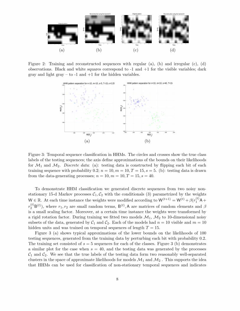
One way to validate correctness of the HHM learning rule is by performing deterministic recon-struction of learned temporal sequences from noiseless initializations at the starting patterns.For discrete sequences we expect such reconstructions to be good if there are sufficiently manyhidden variables to capture long temporal dependencies, i.e. if the total number of nodes is ofthe same order as s× T (the number of training sequences and their length respectively).

Figures 2 (a), (b) illustrate reconstruction of a 7-d discrete time series of length 15, per-formed by a network with 7 visible and 3 hidden units1. The initial training pattern v(0) was setat uniform random, and each subsequent observation vector v(t+1) was generated from v(t) byflipping each bit with probability 0.2 [Figure 2 (a)]. The model parameters Θ were learned bythe EM algorithm (section 3). The reconstructed sequence was generated from the initial statex(0), sampled from the learned prior p(x(0)), by deterministically setting subsequent variables

x(t+1)i according to sgn(σ(x

(t+1)i (wT

i x+bi))−1/2) [Figure 2 (b)]. Note that without hidden vari-ables deterministic reconstruction of the visible training sequence would be impossible. Indeed,patterns v(7) and v(8) are identical, and it is the learned activation of the hidden variables h(7)

and h(8) which distinguishes mapping x(7) → x(8) from x(8) → x(9).Figures 2 (c), (d) show a variant of the previous experiment for a discrete 10-d time series

with irregularly missing data. It is pleasing that the model perfectly reproduces the visiblepatterns, although nothing in the framework explicitly suggests perfect reconstruction of thehidden variables from noisy initialization at the starting visible state.

Note that in order to deterministically reconstruct a binary sequence in HHMs it is sufficient

to ensure that each data point v(t)i maps into v

(t+1)i lying on the correct side of the hyperplane

(wi; bi). Reconstruction of continuous temporally correlated patterns is in general more complex.

5.2 Classification of discrete sequences

In large scale HHMs computation of the likelihood of a sequence is intractable. One possiblediscriminative criterion for classification of a given new sequence v? is the lower bound on thelikelihood Φ(v?; q?,Θ) given by expression (2). Once HHM parameters Θ are optimized for thetraining set {v}, the distribution q? may be evaluated by fixing Θ, clamping v? on the visiblevariables, and performing just the E-step of the algorithm.

1From now on we imply multiplication of the network size by the sequence length T .

7

Original pattern

TimeN

ode

1 3 5 7 9 11 13

1

2

3

4

5

6

7

Reconstruction using the learned Θ

Time

No

de

1 3 5 7 9 11 13

1

2

3

4

5

6

7

8

9

10

Original pattern

Time

No

de

1 3 5 7 9 11 13

1

2

3

4

5

6

7

8

9

10

Reconstruction using the learned Θ

Time

No

de

1 3 5 7 9 11 13

1

2

3

4

5

6

7

8

9

10

(a) (b) (c) (d)

Figure 2: Training and reconstructed sequences with regular (a), (b) and irregular (c), (d)observations. Black and white squares correspond to -1 and +1 for the visible variables; darkgray and light gray – to -1 and +1 for the hidden variables.

−300 −280 −260 −240 −220

−300

−280

−260

−240

−220HHM pattern separation for n=10, m=10, s=5, T=15, ε=0.20

Φ(Θ1)

Φ(Θ

2)

−350 −340 −330 −320 −310 −300 −290−350

−340

−330

−320

−310

−300

−290HHM pattern separation for n=10, m=10, s=40, T=15

Φ(Θ1)

Φ(Θ

2)

(a) (b)

Figure 3: Temporal sequence classification in HHMs. The circles and crosses show the true classlabels of the testing sequences; the axis define approximations of the bounds on their likelihoodsfor M1 and M2. Discrete data: (a): testing data is constructed by flipping each bit of eachtraining sequence with probability 0.2; n = 10,m = 10, T = 15, s = 5. (b): testing data is drawnfrom the data-generating processes; n = 10,m = 10, T = 15, s = 40.

To demonstrate HHM classification we generated discrete sequences from two noisy non-stationary 15-d Markov processes C1, C2 with the conditionals (3) parametrized by the weights

W ∈ R. At each time instance the weights were modified according to W(t+1) = W(t)+β(r(t)1 A+

r(t)2 B(t)), where r1, r2 are small random terms, B(t),A are matrices of random elements and βis a small scaling factor. Moreover, at a certain time instance the weights were transformed bya rigid rotation factor. During training we fitted two modelsM1,M2 to 10-dimensional noisysubsets of the data, generated by C1 and C2. Each of the models had n = 10 visible and m = 10hidden units and was trained on temporal sequences of length T = 15.

Figure 3 (a) shows typical approximations of the lower bounds on the likelihoods of 100testing sequences, generated from the training data by perturbing each bit with probability 0.2.The training set consisted of s = 5 sequences for each of the classes. Figure 3 (b) demonstratesa similar plot for the case when s = 40, and the testing data was generated by the processesC1 and C2. We see that the true labels of the testing data form two reasonably well-separatedclusters in the space of approximate likelihoods for modelsM1 andM2 . This supports the ideathat HHMs can be used for classification of non-stationary temporal sequences and indicates

8

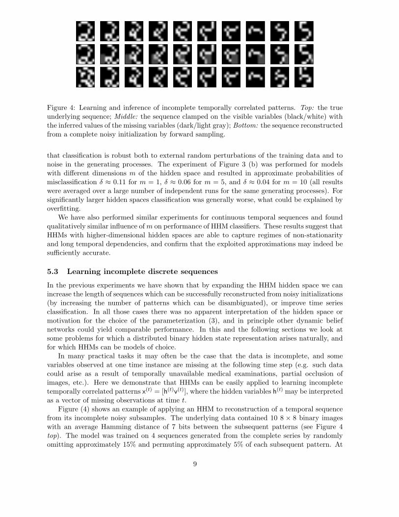
Figure 4: Learning and inference of incomplete temporally correlated patterns. Top: the trueunderlying sequence; Middle: the sequence clamped on the visible variables (black/white) withthe inferred values of the missing variables (dark/light gray); Bottom: the sequence reconstructedfrom a complete noisy initialization by forward sampling.

that classification is robust both to external random perturbations of the training data and tonoise in the generating processes. The experiment of Figure 3 (b) was performed for modelswith different dimensions m of the hidden space and resulted in approximate probabilities ofmisclassification δ ≈ 0.11 for m = 1, δ ≈ 0.06 for m = 5, and δ ≈ 0.04 for m = 10 (all resultswere averaged over a large number of independent runs for the same generating processes). Forsignificantly larger hidden spaces classification was generally worse, what could be explained byoverfitting.

We have also performed similar experiments for continuous temporal sequences and foundqualitatively similar influence ofm on performance of HHM classifiers. These results suggest thatHHMs with higher-dimensional hidden spaces are able to capture regimes of non-stationarityand long temporal dependencies, and confirm that the exploited approximations may indeed besufficiently accurate.

5.3 Learning incomplete discrete sequences

In the previous experiments we have shown that by expanding the HHM hidden space we canincrease the length of sequences which can be successfully reconstructed from noisy initializations(by increasing the number of patterns which can be disambiguated), or improve time seriesclassification. In all those cases there was no apparent interpretation of the hidden space ormotivation for the choice of the parameterization (3), and in principle other dynamic beliefnetworks could yield comparable performance. In this and the following sections we look atsome problems for which a distributed binary hidden state representation arises naturally, andfor which HHMs can be models of choice.

In many practical tasks it may often be the case that the data is incomplete, and somevariables observed at one time instance are missing at the following time step (e.g. such datacould arise as a result of temporally unavailable medical examinations, partial occlusion ofimages, etc.). Here we demonstrate that HHMs can be easily applied to learning incompletetemporally correlated patterns x(t) = [h(t)v(t)], where the hidden variables h(t) may be interpretedas a vector of missing observations at time t.

Figure (4) shows an example of applying an HHM to reconstruction of a temporal sequencefrom its incomplete noisy subsamples. The underlying data contained 10 8 × 8 binary imageswith an average Hamming distance of 7 bits between the subsequent patterns (see Figure 4top). The model was trained on 4 sequences generated from the complete series by randomlyomitting approximately 15% and permuting approximately 5% of each subsequent pattern. At

9

the reconstruction stage the visible part of the sequence with different, systematically missingobservations, was clamped on the HHM’s visible units, and the missing observations were inferredvariationally. As we see from Figure 4middle, the resulting reconstruction is reasonably accurate.

We have also tried to retrieve the underlying sequence by deterministic forward sampling(Figure 4 bottom) as described in section (5.1). The model was initialized at the completely

visible starting pattern x(0) perturbed with 10% noise. Each subsequent pattern x(t+1)i was

set according to sgn(σ(x(t+1)i (wT

i x(t) + bi)) − 1/2) and perturbed with additional 10% noise.We see that the underlying sequence can still be retrieved relatively accurately, though furtherexperiments show that this reconstruction proves to be sensitive to the noise of the trainingsequences.

5.4 Constrained HHMs for sequence halftoning

As we noted in section 3.4, learning all (m+n)×(m+n) weights could often be prohibitive. Oneway to circumvent this problem is to impose sparsity constraints on the weight matrix, so thatthe transitions and emissions are defined by a small subset of the full weight matrix. In additionto decreasing computational effort and reducing the required amount of training data, carefullyimposed constraints may yield a clear topological interpretation of the hidden variables.

Consider, for example, a special case of a generalized Markov chain with the joint distributiongiven by

p({h}, {v}) = p(h(0))T−1∏

t=0

p(h(t+1)|h(t))p(v(t+1)|h(t)). (18)

Graphically, the model corresponds to an HMM with a high-dimensional distributed hiddenspace representation. For some types of data (e.g. video sequences) it may be natural to assumethat points which are spatially close to each other belong to the same object, and their colorsare marginally dependent (assuming the objects are reasonably smoothly colored). On theother hand, colors of spatially distant points are likely to be marginally independent. From asingle time slice of the model (18) it is clear that visible variables are marginally dependent ifthey share a common ancestor. By arranging parents sharing common children to be spatiallyclose to each other in the hidden space, we can model smoothness of images by imposing localneighborhood constraints on the emission weights (so that each hidden parent is connected onlyto a small spacial neighborhood in the visible space, and each visible node is a direct offspringof a spacial neighborhood in the hidden space). Moreover, from the graphical structure it isclear that smooth transitions in the hidden space imply smoothness of dynamical changes inobservations and vice versa, yielding local neighborhood constraints on the transition weights.In the extreme case of factorial transitions, marginal dependencies of the visible variables aretime-invariant.

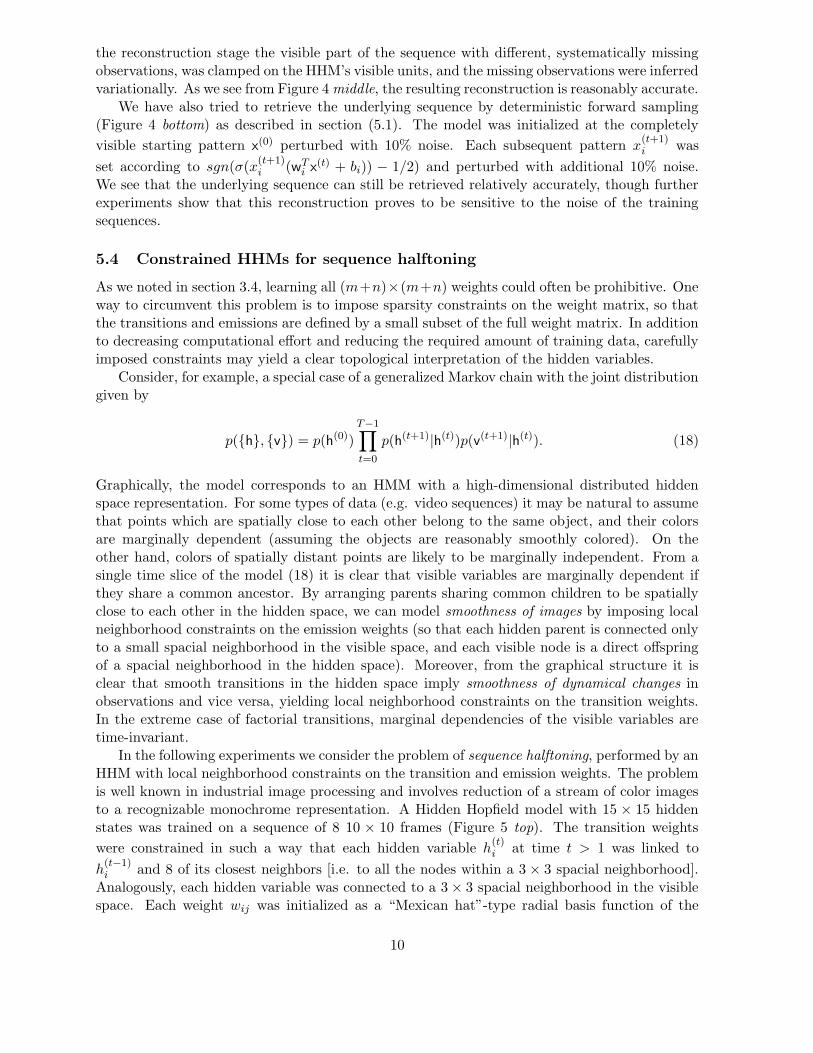
In the following experiments we consider the problem of sequence halftoning, performed by anHHM with local neighborhood constraints on the transition and emission weights. The problemis well known in industrial image processing and involves reduction of a stream of color imagesto a recognizable monochrome representation. A Hidden Hopfield model with 15 × 15 hiddenstates was trained on a sequence of 8 10 × 10 frames (Figure 5 top). The transition weights

were constrained in such a way that each hidden variable h(t)i at time t > 1 was linked to

h(t−1)i and 8 of its closest neighbors [i.e. to all the nodes within a 3 × 3 spacial neighborhood].

Analogously, each hidden variable was connected to a 3× 3 spacial neighborhood in the visiblespace. Each weight wij was initialized as a “Mexican hat”-type radial basis function of the

10

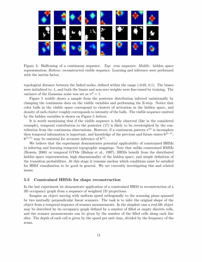
Figure 5: Halftoning of a continuous sequence. Top: true sequence; Middle: hidden spacerepresentation; Bottom: reconstructed visible sequence. Learning and inference were performedwith the inertia factor.

topological distance between the linked nodes, defined within the range (-0.05, 0.1). The biaseswere initialized to -1, and both the biases and non-zero weights were fine-tuned by training. Thevariance of the Gaussian noise was set as σ2 = 1.

Figure 5 middle shows a sample from the posterior distribution inferred variationally byclamping the continuous data on the visible variables and performing the E-step. Notice thatcolor balls in the visible space correspond to clusters of activation in the hidden space, anddensity of each cluster roughly corresponds to intensity of the balls. The visible sequence emittedby the hidden variables is shown on Figure 5 bottom.

It is worth mentioning that if the visible sequence is fully observed (like in the consideredexample), temporal contribution to the posterior (17) is likely to be overweighted by the con-tribution from the continuous observations. However, if a continuous pattern v(t) is incompletethen temporal information is important, and knowledge of the previous and future states h(t−1),h(t+1) may be essential for accurate inference of h(t).

We believe that the experiment demonstrates potential applicability of constrained HHMsto inferring and learning temporal topographic mappings. Note that unlike constrained HMMs(Roweis, 2000) or temporal GTMs (Bishop et al., 1997), HHMs benefit from the distributedhidden space representation, high dimensionality of the hidden space, and simple definition ofthe transition probabilities. At this stage it remains unclear which conditions must be satisfiedfor HHM visualization to be good in general. We are currently investigating this and relatedissues.

5.5 Constrained HHMs for shape reconstruction

In the last experiment we demonstrate application of a constrained HHM to reconstruction of a3D occupancy graph from a sequence of weighted 1D projections.

Imagine an object moving with uniform speed orthogonally to the scanning plane spannedby two mutually perpendicular linear scanners. The task is to infer the original shape of theobject from a temporal sequence of scanner measurements. In the simplest case a real-life objectmay be described by its occupancy graph defined by a number of filled or empty discrete cells,and the scanner measurements can be given by the number of the filled cells along each lineslice. The depth of each cell is given by the speed per unit time, divided by the frequency of thescans.

11

0 2 4 6 8 10 12 14

1

2

3

4

5

6

7

8

9

2

4

6

8

10

0 2 4 6 8 10 12 14

1

2

3

4

5

6

7

8

9

0

5

10

15

0 2 4 6 8 10 12 14

1

2

3

4

5

6

7

8

9

2

4

6

8

10

12

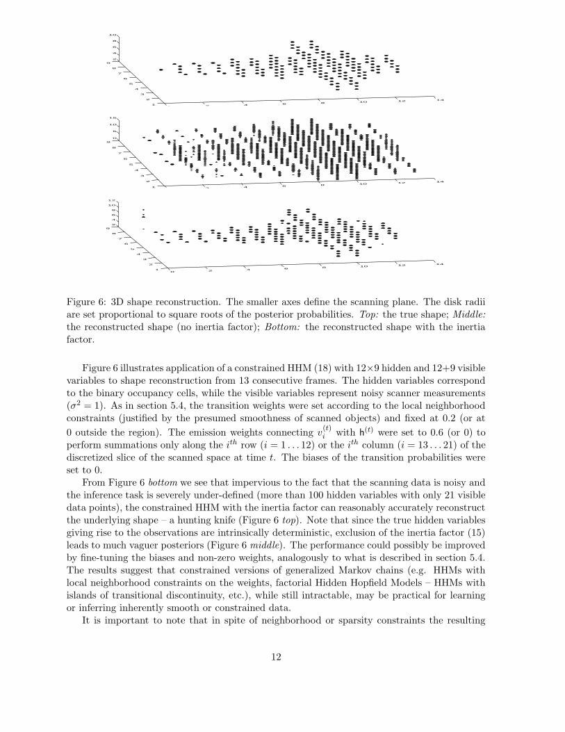
Figure 6: 3D shape reconstruction. The smaller axes define the scanning plane. The disk radiiare set proportional to square roots of the posterior probabilities. Top: the true shape; Middle:

the reconstructed shape (no inertia factor); Bottom: the reconstructed shape with the inertiafactor.

Figure 6 illustrates application of a constrained HHM (18) with 12×9 hidden and 12+9 visiblevariables to shape reconstruction from 13 consecutive frames. The hidden variables correspondto the binary occupancy cells, while the visible variables represent noisy scanner measurements(σ2 = 1). As in section 5.4, the transition weights were set according to the local neighborhoodconstraints (justified by the presumed smoothness of scanned objects) and fixed at 0.2 (or at

0 outside the region). The emission weights connecting v(t)i with h(t) were set to 0.6 (or 0) to

perform summations only along the ith row (i = 1 . . . 12) or the ith column (i = 13 . . . 21) of thediscretized slice of the scanned space at time t. The biases of the transition probabilities wereset to 0.

From Figure 6 bottom we see that impervious to the fact that the scanning data is noisy andthe inference task is severely under-defined (more than 100 hidden variables with only 21 visibledata points), the constrained HHM with the inertia factor can reasonably accurately reconstructthe underlying shape – a hunting knife (Figure 6 top). Note that since the true hidden variablesgiving rise to the observations are intrinsically deterministic, exclusion of the inertia factor (15)leads to much vaguer posteriors (Figure 6 middle). The performance could possibly be improvedby fine-tuning the biases and non-zero weights, analogously to what is described in section 5.4.The results suggest that constrained versions of generalized Markov chains (e.g. HHMs withlocal neighborhood constraints on the weights, factorial Hidden Hopfield Models – HHMs withislands of transitional discontinuity, etc.), while still intractable, may be practical for learningor inferring inherently smooth or constrained data.

It is important to note that in spite of neighborhood or sparsity constraints the resulting

12

HHMs very quickly become intractable. For the 3× 3 topological neighborhoods, the field con-tributions could be calculated exactly (though, as we see, the Gaussian field approximation alsoyields accurate predictions). However, the complexity of exact computations grows exponen-tially with the size of the neighborhood, and for the next closest 5×5 square region (225 possibleparental states) an approximation should be used for most practical purposes. This suggestspossible combinations of exact and approximate methods in sparse HHMs.

6 Summary

Learning temporal sequences with discrete hidden units is typically achieved using only lowdimensional hidden spaces due to the exponential increase in learning complexity with thehidden unit dimension. Motivated by the observation that mean field methods work well in thecounter-intuitive limit of a large, densely connected graph with conditional probability tablesdependent on a linear combination of parental states, we formulated the Hidden Hopfield Modelfor which the hidden unit dynamics is specified precisely by a form for which mean field theoriesmay be accurate in large scale systems. For discrete or continuous observations, we derivedfast EM-like algorithms exploiting mean and Gaussian field approximations, and demonstratedsuccessful applications to classification and reconstruction of non-stationary and incompletecorrelated temporal sequences. We have also discussed learning and inference applications of theconstrained HHMs, which may be useful for learning smooth data. The models can be modified

to allow other types of emission probabilities p(v(t+1)i |v(t), h(t)), e.g. mixtures of Gaussians, or

extended to handling mixed discrete and continuous observations.

A Appendix: Derivations

Here we briefly outline derivation of the variational EM algorithm and the block Gibbs samplingscheme discussed in section 3. The derivations are quite straight-forward; we include them herefor completeness.

A.1 Variational EM algorithm

Let x(t)i be the ith variable of an HHM-induced chain at time t. For each such variable we

introduce an auxiliary parameter λ(t)i , such that λ

(t)i

def= q(x

(t)i = 1) ∈ [0, 1] if x

(t)i is hidden, and

λ(t)i

def= (x

(t)i + 1)/2 (19)

if x(t)i is observable2. If xi is hidden the parameter λ

(t)i must be learned from data, which

is equivalent to the E-step of the variational EM algorithm. Otherwise, λ(t)i is necessarily

deterministic with λ(t)i ∈ {0, 1} for discrete and λ

(t)i ∈ R for continuous observations.

A.1.1 Discrete observations

It is intuitively clear that the parameters λ(t)i corresponding to the visible variables need to

remain fixed, which is equivalent to clamping training sequences on the visible nodes. There areno other principle differences between treating binary hidden and binary visible variables in theconsidered framework.

2To simplify the notation we let xT def

= [hTv

T ] and q({x})def= q({h}|{v}).

13

E-step:

The E-step involves optimization of the lower bound on the likelihood w.r.t. the parametersof the variational distribution q({h}).

From (1) and (2) it is clear that

log p({v}|h(0), v(0)) ≥

|{h}|∑

i=1

H(qi(hi)) +

T−1∑

t=0

〈log p(v(t+1), h(t+1)|v(t), h(t))〉q(h(t),h(t+1)) (20)

where H(qi(hi)) is the entropy of the mean field distribution of qi(hi). Differentiation w.r.t.

q(h(t)k ) leads to

q(h(t)k ) ∝ exp

〈log p(h(t)k |x

(t−1))〉q(h(t−1)) +∑

i∈V (t+1)

〈log p(v(t+1)i |x(t))〉

q(h(t)\h(t)k

)

+∑

m∈H(t+1)

〈log p(h(t+1)m |x(t))〉

q(h(t+1)m ,h(t)\h

(t)k

)

(21)

for each non-starting and non-ending hidden node h(t)k , where V (t+1) and H(t+1) are sets of nodes

visible and hidden at t + 1. From the parameterization given by (3) it is easily derived that

λ(t)k

def= q(h

(t)k = 1) = σ(lk), where

l(t)k = wT

k (2λ(t−1) − 1) + bk +

∑

i∈V (t+1)

[

〈log σ(v(t+1)i ctik)〉p(ct

ik) − 〈log σ(v

(t+1)i dtik)〉p(dt

ik)

]

+∑

m∈H(t+1)

[

⟨

log{

σ(ctmk)λ(t+1)i σ(−ctmk)

1−λ(t+1)m

}⟩

p(ctmk

)

−⟨

log{

σ(dtmk)λ(t+1)m σ(−dtmk)

1−λ(t+1)m

}⟩

p(dtmk

)

]

(22)

and the fields ctmk and dtmk are given by

ctmk = wTmx(t) + bm|h

(t)k = 1, (23)

dtmk = wTmx(t) + bm|h

(t)k = −1. (24)

Since ctmk and dtmk are given by linear combinations of random variables, the Central LimitTheorem implies approximate Gaussianity of p(ctmk) and p(dtmk) (Barber and Sollich, 2000)with the means µcmk(t), µ

dmk(t) trivially given by

µdmk(t) = wTm(2λ

(t) − 1)− 2wmkλ(t)k + bm, (25)

µcmk(t) = µdmk(t) + 2wmk (26)

and the variances

sdmk(t) = scmk(t) =

⟨

∑

i6=k

wmi(x(t)i − 〈x

(t)i 〉)

2⟩

=∑

i,j 6=k

wmiwmj

(

〈x(t)l x

(t)j 〉 − 〈x

(t)l 〉〈x

(t)j 〉)

= 4∑

i6=k

w2mi(1− λ

(t)i )λ

(t)i . (27)

14

Here we have used the mean field approximation 〈xixj〉 = 〈xi〉〈xj〉 and the fact that 〈x2j 〉 = 1.

Thus, the field update (22) may be re-written as

l(t)k ≈ wT

k (2λ(t−1) − 1) + bk +

|x(t)|∑

i=1

⟨

log{

σ(ctik)λ(t+1)i σ(−ctik)

1−λ(t+1)i

}⟩

N cik

(t)

−

|x(t)|∑

i=1

⟨

log{

σ(dtik)λ(t+1)i σ(−dtik)

1−λ(t+1)i

}⟩

N dik

(t), (28)

reducing to

λ(t)k ≈ σ

bk + wTk (2λ

(t−1) − 1) +

|x(t)|∑

i=1

[

logσ(µcik(t))

σ(µdik(t))− 2wik(1− λ

(t+1)i )

]

(29)

when the integrals are approximated at the means.M-step:

The M-step optimizes the lower bound on the likelihood w.r.t. the parameters W and b ofthe conditional distributions (3).

Let wij be the weight connecting x(t+1)i and x

(t)j . From (20) and (3) we get

∂Φ

∂wij=

∂

∂wij

T−1∑

t=0

|x(t+1)|∑

k=1

⟨

log{

σ(

x(t+1)k [wT

k x(t) + bk])}⟩

q(x(t+1)k

,x(t))

=

T−1∑

t=0

⟨(

1− σ(

x(t+1)i [wT

i x(t) + bi]))

x(t+1)i x

(t)j

⟩

q(x(t+1)i ,x(t))

=T−1∑

t=0

[

(2λ(t)j − 1)λ

(t+1)i −

⟨

x(t)j σ

(

wTi x(t) + bi

)⟩

q(x(t))

]

. (30)

Once again applying the Central Limit Theorem, we obtain

∂Φ

∂wij≈

T−1∑

t=0

{

λ(t+1)i (2λ

(t)j − 1)−

[

λ(t)j 〈σ(c

tij)〉N c

ij(t)+ (λ

(t)j − 1)〈σ(dtij)〉N d

ij(t)

]}

(31)

with the moments of N cij(t) and N

dij(t) given by (25) – (27). Analogously,

∂Φ

∂bi=

T−1∑

t=0

⟨(

1− σ(x(t+1)i [wT

i x(t) + bi]))

x(t+1)i

⟩

q(x(t+1)i ,x(t))

=T−1∑

t=0

[

λ(t+1)i − 〈σ(wT

i x(t) + bi)〉q(x(t))

]

≈T−1∑

t=0

[

λ(t+1)i − 〈σ(eti)〉N e

i (t)

]

(32)

where N ei (t) is a Gaussian with the mean and the variance

µei (t) = wTi (2λ

(t) − 1) + bi, (33)

sei (t) = 4

|x(t)|∑

k=1

λ(t)k (1− λ

(t)k )w2

ik. (34)

15

A.1.2 Continuous observations

The derivation is fully analogous to the one described in Appendix A.1.1, with the slight differ-

ences due to parameterization of the conditionals p(v(t+1)i |x(t)) ∼ N (wT

i x(t), s2).E-step:

From (21) we obtain λ(t)k = σ(lk) with

l(t)k = lk

(t)−

1

2s2

∑

i∈V (t+1)

⟨

(v(t+1)i − wT

i x|hk = 1)2 − (v(t+1)i − wT

i x|hk = −1)2⟩

q(x(t))

= lk(t)−

2

s2

∑

i∈V (t+1)

wik

[

wTi (2λ

(t) − 1)− wik(2λ(t)k − 1)− v

(t+1)i

]

, (35)

where

lk(t)

= wTk (2λ

(t−1)k − 1) + bk +

∑

m∈H(t+1)

[

⟨

log{

σ(ctmk)λ(t+1)i σ(−ctmk)

1−λ(t+1)m

}⟩

N cij(t)

−⟨

log{

σ(dtmk)λ(t+1)m σ(−dtmk)

1−λ(t+1)m

}⟩

N dij(t)

]

. (36)

As before, ctmk and ddmk are given by (23) and (24), the moments of N cij(t) and N

dij(t) – by (25) –

(27), and it is assumed that only those parameters λk which correspond to the hidden variablesneed to be adapted.M-step:

By analogy with the previous case, optimization of the upper bound w.r.t. the model pa-rameters leads to

∂Φ

∂wij= −

1

2s2

∂

∂wij

T−1∑

t=0

∑

l∈V (t+1)

〈(wTl x− v

(t+1)l )2〉q(x(t))

+∂

∂wij

∑

k∈H(t+1)

⟨

log{

σ(

x(t+1)k [wT

k x(t) + bk])}⟩

q(x(t+1)k

,x(t)). (37)

There are four possible simplifications of this expression, depending on observability of nodes

x(t+1)i and x

(t)j connected by the weight wij , so that

i ∈ V (t+1), j ∈ H(t) ⇒

∂Φ

∂wij= −

1

s2

T−1∑

t=0

〈(wTi x− v

(t+1)i )x

(t)j 〉q(x(t))

=1

s2

v(t+1)i (2λj − 1)−

|x(t)|∑

k=1

wik〈x(t)k x

(t)j 〉q(x(t))

=1

s2

(

(2λ(t)j − 1)

[

v(t+1)i − wT

i (2λ(t) − 1)

]

+ 4wij(λ(t)j − 1)λ

(t)j

)

, (38)

i ∈ V (t+1), j ∈ V (t) ⇒

∂Φ

∂wij=

1

s2

(

v(t)j

[

v(t+1)i − wT

i (2λ(t) − 1)

])

, (39)

16

i ∈ H(t+1), j ∈ V (t) ⇒

∂Φ

∂wij= v

(t)j

[

λ(t+1)i − 〈σ(wT

i x + bi)〉q(x)

]

≈ v(t)j

[

λ(t+1)i − 〈σ(eti)〉N e

i (t)

]

, (40)

where the moments of eti ∼ Nei (t) are given by (33) – (34). Finally, in the last case when

i ∈ H(t+1), j ∈ H(t) the gradients ∂Φ/∂wij are given by (31). Note that all of the abovegradients can be combined to give (6), and ∂Φ/∂bi is expressed as (32).

A.2 Gibbs sampling

Here we derive the conditional distributions used in the sampling scheme outlined in section 4.Let X and X be the odd layers of a 3-layer fully-connected chain X → X → X. We are

interested in sampling the even layer X from p(X|X, X). Note that p(X,X, X) = p(X)p(X|X)p(X|X),i.e.

p(X|X, X) ∝ p(X|X)p(X|X) =∏

i

p(Xi|X)p(X|X\i, Xi). (41)

Here Xi is a hidden variable in layer X, and X\idef= X\Xi. Note that in general p(X|X\i, Xi) is

not factorized over Xis. This complicates normalization of (41) and motivates usage of anothersampler for X’s components

Xi ← p(Xi|X\i, X, X) ∝ p(Xi,X

\i|X)p(X|X\i, Xi)

∝ p(Xi|X)∏

j

p(Xj |X\i, Xi), (42)

where we have used (41) and the fact that p(Xi|X\i, X) = p(Xi|X).

For the HHMs, the conditional distributions of the hidden variables p(h(t+1)i |x(t)) are given

by (3), and the conditional distributions of the visible variables p(v(t+1)i |x(t)) ∼ N (wT

i x(t), s2).From (42) it is then clear that

p(h(t)i = ±1|x(t−1), x(t+1), x(t)\h

(t)i ) ∝

σ(±[wTi x(t−1) + bi])

|h(t+1)|∏

j=1

σ(h(t+1)j [wT

j x(t) − wjix(t)i ± wji])

|v(t+1)|∏

k=1

exp

{

−1

2s2(v

(t+1)k − [wT

k x− wkix(t)i ± wki])

2

}

, (43)

which leads to

x(t)i ← p(x

(t)i = 1|x(t−1), x(t+1), x(t)\x

(t)i ) =

σ

bi + wTi x(t−1) +

|x(t+1)|∑

j=1

logσ(

x(t+1)j

[

wTi x− wjixi + wji)

]

)

σ(

x(t+1)j

[

wTi x− wjixi − wji)

]

)

(44)

17

for discrete and

x(t)i ← p(x

(t)i = 1|x(t−1), x(t+1), x(t)\x

(t)i ) =

σ

bi + wTi x(t−1) +

|h(t+1)|∑

j=1

logσ(

x(t+1)j

[

wTi x− wjixi + wji)

]

)

σ(

x(t+1)j

[

wTi x− wjixi − wji)

]

)

+2

σ2

|v(t+1)|∑

k=1

wki

(

v(t+1)k − wT

k x(t) + wkih(t)i

)

(45)

for continuous data models. Here we have used simple identities a/(a + b) ≡ σ(log(a/b)) andlog(σ(a)/σ(−a)) ≡ a which hold ∀a, b > 0.

References

Barber, D. and Sollich, P. (2000). Gaussian Fields for Approximate Inference. In Solla, S. A., Leen, T.,and Muller, K.-R., editors, Advances in Neural Information Processing Systems 12, pages 393–399.MIT Press, Cambridge, MA.

Bishop, C. M., Hinton, G. E., and Strachan, I. G. D. (1997). GTM Through Time. NCRG/97/005,NCRG, Dept. of Computer Science and Applied Mathematics, Aston University.

Ghahramani, Z. and Jordan, M. (1995). Factorial hidden Markov models. In Touretzky, D. S., Mozer,M. C., and Hasselmo, M. E., editors, Proc. Conf. Advances in Neural Information Processing Systems,

NIPS, volume 8, pages 472–478. MIT Press.

Hertz, J., Krogh, A., and Palmer, R. G. (1991). Introduction to the Theory of Neural Computation. MA:Addison-Wesley Publishing Company.

Neal, R. M. (1992). Connectionist learning of belief networks. Artificial Intelligence, (56):71 – 113.

Rabiner, L. (1989). A tutorial on hidden Markov models and selected applications in speech recognition.Proc. of the IEEE, 77(2).

Roweis, S. (2000). Constrained hidden Markov models. In Proc. Conf. Advances in Neural Information

Processing Systems, NIPS, volume 12. MIT Press.

Saul, L., Jaakkola, T., and Jordan, M. (1996). Mean field theory for sigmoid belief networks. Journal ofArtificial Intelligence Research, 4.

18