school of engineering - university of nairobi
TRANSCRIPT

i
UNIVERSITY OF NAIROBI
SCHOOL OF ENGINEERING
Department of Electrical and Information Engineering
MSc(Electrical and Electronic Engineering)
POWER LOSS REDUCTION IN THE DISTRIBUTION
SYSTEM WITH A WIND BASED DISTRIBUTED
GENERATION
By
Moses Peter Musau
F56/60213/2011
BSc (Electrical and Electronics Engineering),The University of Nairobi.
A Thesis submitted in partial fulfilment for the degree of Master of Science in the
Department of Electrical and Information Engineering of the University of
Nairobi.
FEBRUARY 2014

ii
DECLARATION OF ORIGINALITY
NAME OF STUDENT: MOSES PETER MUSAU
REGISTRATION NUMBER: F56/60213/2011
COLLEGE: Architecture and Engineering
FACULTY/SCHOOL/INSTITUTE: School of Engineering
DEPARTMENT: Electrical and Information Engineering
COURSE NAME: Master of Science in Electrical and Electronic Engineering
TITLE OF WORK: POWER LOSS REDUCTION IN THE DISTRIBUTION
SYSTEM WITH A WIND BASED DISTRIBUTED GENERATION.
1) I understand what plagiarism is and I am aware of the university policy in this regard.
2) I declare that this Master of Science in Electrical and Electronic Engineering
Thesis is my original work and has not been submitted elsewhere for examination,
award of a degree or publication. Where other people’s work or my own work
has been used, this has properly been acknowledged and referenced in
accordance with the University of Nairobi’s requirements.
3) I have not sought or used the services of any professional agencies to produce this work.
4) I have not allowed, and shall not allow anyone to copy my work with the
intention of passing it off as his/her own work.
5) I understand that any false claim in respect of this work shall result in
disciplinary action, in accordance with University anti-plagiarism policy.
Signature:
……………………………………………………………………………………
Date:
………………………………………………………………………………………

iii
DECLARATION
I Moses Peter Musau hereby declare that this thesis is my original work. To the best of my
knowledge, the work has not been presented for a degree award in The University of Nairobi or
any other Institution of Higher Learning.
Sign:………………………………
Date:……/…………/……………
Peter Musau Moses
Reg No: F56/60213/2011
This MSc Research thesis has been submitted to the School of Engineering, Department of
Electrical and Information Engineering, The University of Nairobi with my approval as The
University Supervisor.
Sign:………………………….……
Date:……/…………/…………….
Dr.N.Abungu

iv
DEDICATION
To my God and The Church.
“Study to show yourself approved to God, a workman that needs not to be
ashamed, rightly dividing the word of truth.” 2 Timothy 2:15 (NKJV)

v
ACKNOWLEDGEMENT
I have been very fortunate to have Dr.Nicodemus Abungu,Senior Lecturer, Department of
Electrical Information Engineering,The University of Nairobi as my thesis supervisor. I am
highly indebted to him and express my deep sense of gratitude for his guidance and valuable
discussion throughout the thesis. He encouraged, supported and motivated me with much
kindness throughout the work. I always had the freedom to follow my own ideas, of which I am
very grateful for him. Truly, this thesis would not have been possible without the fruitful
comments, suggestions and support from him. I really admire him for patience and staying power
to carefully read the whole manuscript.
I express my sincere gratitude to the academic and support staff members of the Department of
Electrical and Information Engineering, for their unparalleled academic support and ideas during
my thesis. These include Celestine waita,Edwin Nganga,Tom Oloo,Duncan Kinuthia and Luke
Wangai.
I do appreciate the Professor Pattis Odira(Dean,School of Engineering),Professor Mwangi
Mbuthia(Internal examiner),Dr Odwesso Muhua.Dr Mbunge Onyango ,Dr.Nicodemus
Abungu(Supervisor and Internal Examiner),Mrs.F.Midamba(Administrative Assistant,Deans
Office) for accepting and acting as the Board of Examiners for this thesis.My heart felt
blessing goes to the external examiner professor Josiah Munda(Associate Dean,Faculty of
Engineering and the Built Enviroment,Tshwane University of Technology) for his thorough
examination of the research work.
I render my respect my dear wife Jackline Mutheu Peter and son Prince Michael for giving me
physical, spiritual, mental support and inspiration for carrying out my research work. Thank you
for being my best friends. I would like to thank my parents Mr. and Mrs. Moses, my dear
brothers and sisters for all their faith and confidence in me to pursue a Master’s program in the
University of Nairobi. I am indebted to them for their unending love and blessings throughout
my work.
vi
ABSTRACT
Distribution system operating environments are changing rapidly due to the integration of the
intermittent renewable in to the power grid at the distribution side of the power system.
Therefore, with increasing number of wind based distributed generators (DFIGs) being installed
within distribution systems, the traditional methods for distribution system modeling, DFIG
placement & sizing, network reconfiguration needs to be reviewed and better practical ones
developed to cater for the intermittent renewable power.
The combined participation factors, realized by the Newton Raphson method, capture network
parameters, load distributions and DFIG capacities (sizes) and locations have been formulated
considering real and reactive power. A distributed slack bus model taking into consideration
network sensitivity is proposed in the research as compared to the distributed slack bus models
based on the DFIG capacity, DFIG domains and the single slack bus model.
DFIG placement and sizing using a particle swarm optimization method (PSO) and a hybrid of
GA and PSO (HGAPSO) and by load flow method are compared. With simulated results, the
optimal location of the DFIG is the primary distribution system, with the HGAPSO giving
improved results as compared to the ordinary PSO and the load flow.
The active distribution network reconfiguration problem with an objective function of reducing
real and reactive power losses in the presence of DFIG and uncertain loads proves the
practicability of such a method in reducing power losses and in improvement of the voltage
profile .Here an hybrid method of bacterial foraging and differential evolution (HBFDE)is
applied.
The proposed methods, as applied to the IEEE 33 Bus Radial distribution system ,are found to
be effective in the power loss reduction in the power system wind based distributed
generation.

vii
TABLE OF CONTENTS
DECLARATION OF ORIGINALITY ................................................................................................................... ii
DECLARATION .............................................................................................................................................. iii
DEDICATION................................................................................................................................................. iv
ACKNOWLEDGEMENT .................................................................................................................................. v
ABSTRACT .................................................................................................................................................... vi
TABLE OF CONTENTS .................................................................................................................................. vii
ABREVIATIONS ........................................................................................................................................ xi
LIST OF FIGURES .................................................................................................................................... xiv
LIST OF TABLES ...................................................................................................................................... xv
Chapter 1 ....................................................................................................................................................... 1
INTRODUCTION ..............................................................................................................................1
1.1 Problem Statement. ..................................................................................................................1
1.2 Justification ..............................................................................................................................2
1.3 Objectives ................................................................................................................................4
1.4 Research Questions ..................................................................................................................4
1.5 Thesis Organization...................................................................................................................5
1.6 Scope of the Research Work ......................................................................................................6
Chapter 2 ....................................................................................................................................................... 7
POWER SYSTEMS OVERVIEW ..........................................................................................................7
2.1 Distribution System ..................................................................................................................7
2.1.1 Typical power system [5] ..............................................................................................7
2.1.2 Power System Buses ....................................................................................................9
2.2 Distributed Generation .............................................................................................................9
2.2.1 Background of Distributed Generation .........................................................................9
2.2.2 Distributed Generation Technologies.......................................................................... 10
2.2.3 Wind Generation Technologies ................................................................................... 10
2.3 Doubly Fed Induction Generators (DFIG) and Reactive Power. ................................................. 11

viii
2.3.1 DFIG Overview ........................................................................................................... 11
2.3.2 Effects of reactive power to Distribution system with DFIG ......................................... 12
2.4 Distribution System Optimization ............................................................................................ 15
2.4.1 Classification of Optimization Techniques ................................................................... 16
2.4.2 Comparison ............................................................................................................... 16
2.5 Chapter Conclusion ................................................................................................................. 18
Chapter 3 ..................................................................................................................................................... 19
DFIG BASED DISTRIBUTED SLACK BUS MODEL ............................................................................... 19
3.1 Participation Factors ......................................................................................................... 19
3.2.1 Back Ground in Power Systems .................................................................................. 19
3.2.2 Real Power Participation Factors ................................................................................ 21
3.2.3 Reactive Power Participation Factors .......................................................................... 22
3.2.4 Penalty Factors .......................................................................................................... 23
3.2.5 Network Sensitivity Combined Participation Factors ................................................... 24
3.2.6 DFIG Domains Combined Participation Factors ........................................................... 28
3.2.7 Applications of Participation Factors in present work ................................................ 29
3.2 Single Slack Bus Model ...................................................................................................... 30
3.3 Distributed Slack Bus Model .............................................................................................. 31
3.3.1 DFIG Based Distributed Slack Bus Model ..................................................................... 32
3.4 Solution Algorithm for Reactive Power Participation Factors .............................................. 33
3.5 Flow Chart for the Solution Algorithm of reactive Power participation factors .................... 36
3.6 Simulation Results and Analysis ......................................................................................... 37
3.7.1 Participation factors and Power loss ................................................................................. 37
3.7.2Voltage Profile .................................................................................................................. 41
3.7 Chapter Conclusion ........................................................................................................... 43
Chapter 4 ..................................................................................................................................................... 45
DFIG PLACEMENT AND SIZING ...................................................................................................... 45
4.1 DG Placement and Sizing ................................................................................................... 45
4.2 DFIG Placement and Sizing ................................................................................................ 46
4.3 The DFIG Capability Limit Curves........................................................................................ 47
4.4 Problem Formulation ........................................................................................................ 50
4.5 HGAPSO Method ............................................................................................................... 54

ix
4.5.1 Particle Swarm Optimization (PSO) ............................................................................. 54
4.5.2 Genetic Algorithm (GA) .............................................................................................. 54
4.5.3 Hybrid of PSO and GA (HGAPSO) ................................................................................ 56
4.6 Proposed HGAPSO Algorithm ............................................................................................ 58
4.7 Results and Analysis .......................................................................................................... 60
4.7.1 Power Loss Reduction ................................................................................................ 60
4.7.2 Bus Voltage Profile ..................................................................................................... 62
4.8 Chapter Conclusion ........................................................................................................... 63
Chapter 5 ..................................................................................................................................................... 65
ACTIVE DISTRIBUTION NETWORK RECONFIGURATION (ADNR) PROBLEM WITH WIND & UNCERTAIN
LOAD ........................................................................................................................................... 65
5.1 Background ....................................................................................................................... 65
5.2 Network Reconfiguration Review ...................................................................................... 66
5.3 ADNR with Wind Based DFIG ............................................................................................. 68
5.4 ADNR Problem Formulation with Wind .............................................................................. 71
5.5 The Stochastic Model of DFIG and Loads ............................................................................ 75
5.6 The HBFDE Algorithm ........................................................................................................ 78
5.6.1 Bacterial Foraging (BF) Algorithm ............................................................................... 79
5.6.2 Differential Evolutionary (DE) Algorithm ..................................................................... 81
5.6.3 The HBFDE Algorithm ............................................................................................... 83
5.7 The ADNR Algorithm with Wind and Load Uncertainty ..................................................... 84
5.7.1 The algorithm for the DFIG scenario generation .......................................................... 84
5.7.2 The HBFDE Algorithm Mechanism .............................................................................. 85
5.8 Simulation Results and Analysis ......................................................................................... 86
5.8.1 The Test Network before and after reconfiguration .................................................... 87
5.8.2 A Comparison of BF DE and HBFDE without DFIG ........................................................ 88
5.8.3 ADNR problem with Wind .......................................................................................... 89
5.8.4 The Voltage Profile .................................................................................................... 92
5.8.5 Comparison with Other Methods ............................................................................... 92
5.9 Chapter Conclusion ........................................................................................................... 93
Chapter 6 ..................................................................................................................................................... 94
CONTRIBUTIONS AND RECOMMENDATIONS ................................................................................. 94

x
6.1 General Conclusions .......................................................................................................... 94
6.2 Comparison ....................................................................................................................... 95
6.3 Contributions .................................................................................................................... 96
6.4 Beneficiaries of this Research Work ................................................................................. 97
6.5 Recommendations for Future Work ................................................................................... 98
REFERENCES ................................................................................................................................. 99
RESEARCH PAPERS OUT OF THE PRESENT WORK PUBLISHED IN INTERNATIONAL JOURNAL .......... 113
APPENDIX A ............................................................................................................................... 114
APPENDIX B ............................................................................................................................... 117

xi
ABREVIATIONS
ABC-Artificial Bee Colony
AC-Alternating Current
ACO -Ant Colony Optimization
ADNR- Active Distribution Network
ADNR- Active Distribution Network Reconfiguration
BF-Bacterial foraging
BPSO-Binary Particle Swarm Optimization
CERTS- Consortium for Electricity Reliability Technology Solutions
CPF-Continuous Power Flow
DE-Differential evolution
DG-Distributed Generator
DGs-Distributed Generators
DIFG-Doubly Fed Induction Generator
DLF- Distribution Load Flow
DNR-Distribution Network Reconfiguration
DPC-Direct Power Control
EP-Evolutionary Programming
EPRI-Electric Power Research Institute
FACTS- Flexible Alternative Current Transmission Systems
FGA-Fuzzy Genetic Algorithm
FL-Fuzzy Logic
FRT-Fault Ride Through
GA-Genetic Algorithm Optimization
GS-Gauss Siedel

xii
HBCO-Honey Bee Colony Optimization
HBFDE- Hybrid of bacterial foraging and Differential evolution
HCBMOP-Hybrid and Constraint Based Multi Objective Programming.
HDP-Heuristic Dynamic Programming
HGAPSO-Hybrid of Genetic Algorithm and Particle Swarm Optimization
HPSOWM-Hybrid Particle Swarm Optimization with Wavelet Mutation
IEEE-Institute of Electrical and Electronics Engineers
INC-Interface Neuro Controller
IPM-Interior Point Method
IPPs-Independent Power Producers
KPLC-Kenya Power Lighting Company
LVRT- Low Voltage Ride Through
MAMD-Multiple Attribute Making Decision
MC-Monte Carlo
MIHDE-Mixer Integer Hybrid Differential Evolution
MINLP-Mixed Integer Non Linear Programming
MOPSO-Multiple Objective Particle Swarm Algorithm
MPPT-Maximum Power Point Tracking
NGF-Natural Gas Foundation
NSGA-Non-Dominated Sorting GA
OPF-Optimal Power Flow
PCC-Point of Common Coupling
PMSG-Permanent Magnet Synchronous Generator
PSO-Particle Swarm Optimization
PWM-Pulse Width Modulation

xiii
RBFNNs-Radial Basis Function Neural Networks
SA-Simulated Annealing
SCIG-Squirrel Cage Induction Generator
SFIG-Singly Fed Induction Generator
SPV-Solar Photo Voltaic
STATCOM-Static Synchronous Compensator
TS-Tabu Search
VSC-Voltage Source Converter
VSHDE-variable scaling hybrid differential evolution
WECC-Wind Energy Control Council
WECS- Wind Energy Control Systems
WTG-Wind Turbine Generator
WT-Wind Turbine

xiv
LIST OF FIGURES
FIGURE NAME PAGE
2.1 Typical Power System 8
2.2 DFIG Schematic Diagram 13
3.1 Flow Chart for the Solution Algorithm of reactive Power participation
factors
36
3.2 Voltage Profile for Real and Combined Participation factors 41
3.3 Voltage Profile for DFIG installations and without DFIG 42
3.4 Voltage Profile with the DFIG based DSB
43
4.1 DFIG Equivalent Circuit 48
4.2 DFIG Capability Limits Curve 50
4.3 Flow chart for HGAPSO Algorithm 60
4.4 Bus Voltages Profile after DFIG Placement using PSO and HGAPSO
and load flow
63
5.1 Discretization of PDF of wind forecast error 74
5.2 Roulette Wheel Selection 76
5.3 Flow Chart for the ADNR Algorithm with wind and load uncertainty. 86
5.4a) 33-Bus IEEE, Radial distribution network in the initial reconfiguration 87
5.4b) 33-Bus IEEE,Radial distribution network after reconfiguration with
DFIG
87
5.5 The profile voltages for Deterministic and Stochastic Scenarios. 92
6.1 A comparison of voltage profile improvement 96

xv
LIST OF TABLES
TABLE NAME PAGE
3.1 Comparison of load flow methods for new distribution networks 34
3.2 33 Bus Radial Distribution System With DFIG on Bus 18 to Service
1500kw 750kvar Load
39
3.3 33 Bus Radial Distribution System With one DFIG on Bus 19 to service
1500KW 750 KVAR Load
40
4.1 1.5 MW DFIG on Bus 18 61
4.2 1.5 MW DFIG on Bus 8 61
4.3 1.5 MW DFIG on Bus 3 62
5.1 Comparison of average solutions of 10 trials without considering DFIGs
88
5.2 The Simulation Results for DFIG in Stochastic Scenario
90
5.3 The optimum results of deterministic and stochastic situations
91
5.4 A Comparison of results obtained by optimizing active power loss 93
6.1 Comparison of loss reduction methods 95

1
Chapter 1
INTRODUCTION
This is an introduction chapter to the research area with a statement of the problem, a
justification of the study, the objectives and the research questions .Finally an organization of the
thesis is outlined.
1.1 Problem Statement.
The traditional Distribution System design has various inherent drawbacks. The design does not
take into account DG introduction especially the intermittent wind based DFIGs. Also the
penalty factors used in economic power dispatch and unit commitment by J.J.Grainger and
W.D Stevenson ,2003,[1] are derived using the method of Lagrange Multipliers without taking
into consideration the reactive power losses. However ,these losses can no longer be ignored in
the commercially viable DFIG used in the integration of wind energy into the grid.
Due to load growth, load demand exceeds the predetermined threshold capacity of distribution
systems; therefore distribution system design should either do an addition of new substations,
DGs or expand the existing substations’ capacities [2]. This must take into consideration the
type, position and the size of the DFIG so as to maintain the system voltage stability. In
modern practical power systems where reactive power injection plays a critical role in voltage
stability control, the reactive power losses need to be incorporated into the load flow problem.
This is not accounted for in the existing literature especially where intermittent renewable like
wind is involved.
2
The method of connecting DG with electric power system affects DG control schemes. The
IEEE Standard 1547 provides the minimum technical requirements of interconnecting
distributed resources with electric power system[3].The requirements are functional
requirements and do not specify any particular connection method or equipments. To achieve
some specified planning and operating goals for a wind based distributed generation through
automatic or manual control, regulation of electric power injections(both real and reactive )
from the DFIGs within power systems is required.
This thesis, therefore, as one of the objectives , has developed combined participation factors
taking in consideration both real and reactive power losses by using DFIG sizing and
locations, network parameters and load distribution parameters. Then a Newton Raphson
algorithm for distributing the slack in a Wind based DFIG Distribution system is formulated
using the combined participation factors. Further, real and reactive loss reduction is done
using a hybrid of GA and PSO (HGAPSO) for DFIG placement &sizing. Finally, the active
network reconfiguration problem is revisited taking into consideration DFIG placement and
uncertain loads using a hybrid of Bacterial Foraging and Differential Evolution (HBFDE).
1.2 Justification
Global wind resource potential is 72TW which is five times the world’s energy use. Only 4-10%
of this resource can be used in an economically viable way(that is a maximum of 7.2TW).As at
5th February 2014,the Global Wind Energy Council(GWEC)[4] statistics revealed that the
global wind installed capacity was 318,137MW,which means a growth of 12.5% from 2013.
This means over 6.90TW (96%) of the economically viable wind energy remains unexploited.
By 2020, 1900 GW (28%) of the viable wind energy will be used economically. Due to this,

3
there is increased penetration of wind energy into the grid with the capability of the wind power
to supply the peak load being 20%.
Statistics from the Kenya Power and Lighting Company (KPLC) indicate that wind energy
constitutes about 20% of the 1700 MW additional power that Kenya is working towards injecting
into the national grid, over the next five years. The Lake Turkana Wind Power Project(LTWPP)
is the largest of the three wind power plants that are expected to roar into life in the next two
years, churning out 300 MW. Using the latest wind turbine technology, LTWP will upon full
commissioning in 2014 will provide reliable and continuous clean power to satisfy up to 17% of
Kenya's total power needs. In the light of these national and world statistics, there is need to
solve the technical challenges facing the integration of wind energy into the power grid at the
distribution side and transmission end of the existing power system.
Wind energy is the world’s most developed renewable energy resource due to the need of
providing energy security and the climatic change problem. Assuming that 10% of households
would install wind turbines at a cost competitive with the grid side electricity at 12 pence 19
cents /KWh by 2020 ,production of 1.5 KWh p.a will save 0.6 million Tonnes of CO2
emission.Also,120.8 GW global wind capacity produce 260Twh and saves 158 Million Tones
of CO2 p.a .Also,20% of the worlds viable wind energy can satisfy the worlds electricity
demand by the year 2020 if the challenges facing its integration to the grid are addressed[4].
The Doubly Fed Induction Generator (DFIG) based wind turbine with variable-speed variable-
pitch control scheme is the most popular wind power generator in the wind power industry and
can be operated either in grid connected or stand alone mode. A thorough understanding of the
modeling, control, and dynamic as well as the steady state analysis of this machine in both

4
operation modes is necessary to optimally extract the power from the wind and accurately predict
its performance. Thus new strategies and methods for distribution system expansion planning
,which include DFIG placement, DFIG sizing and network reconfiguration , need to be studied.
1.3 Objectives
The main objective of this research is to optimize real and reactive losses in the presence of the
DFIG.The objective is further divided in to the following sub objectives:
To formulate combined participation factors for reactive and real power loss allocation
for DFIGs.
To formulate a distributed slack bus model for the distribution system with DFIGs.
To evaluate the impacts of introducing distributed slack bus models for reactive power
loss to wind based DFIG placement and sizing.
To design new strategies for network reconfiguration with wind based DFIG and
uncertain loads.
1.4 Research Questions
The following research questions have been addressed so as to fulfill the objectives:
How can the reactive power loss participation factors for DFIGs be formulated?
What are the differences between the participation factors of reactive power and real
power loss contributions and how can these kinds of participation factors is combined to
form a combined participation factor?
How can reactive power loss distribution to a distributed slack bus model be applied
in power flow study?

5
How can an Algorithm for DFIG placement and sizing be formulated?
How does the presence of the Wind based DFIG in the power grid affect the
Distribution Network reconfiguration problem?
1.5 Thesis Organization
This thesis has six chapters. Chapter 1 is an introduction to the research area ,a statement of the
problem , a justification of the study .Then, the objectives and the research questions are
presented .Finally an organization of the thesis is outlined.
In Chapter 2 a general overview of the power system is done beginning with the typical power
system, the distribution system, distributed generation, wind based distributed generation
technologies, Reactive power and power systems optimization.
Chapter 3 brings out the combined participation factors and the NR based distributed slack
bus model with DFIGs.A background for the participation factors is first given then the real
reactive and the combined participation factors. DFIG based network sensitive and DFIG
distributed slack domain based participation factors are presented and their corresponding
distributed slack bus modes with DFIG compared. The Voltage profiles for all the DFIG based
DSBMs are compared and finally a chapter conclusion is given.
In Chapter 4 the DFIG placement and sizing problem is solved using an hybrid of GA and PSO
(HGAPSO) and the results compared with those obtained by doing the placement using load
flow and ordinary PSO.A chapter conclusion is then drawn.
Chapter 5 deals with active distribution network reconfiguration problem taking into
consideration wind based DFIG and uncertain loads. A hybrid of bacterial foraging (BF) and

6
Differential evolution (DE) (HBFDE) is formulated and then applied for a stochastic wind
scenario and the results compared with those of a deterministic case. The voltage profiles are
also compared and a chapter conclusion is made.
In chapter 6 general thesis conclusions are made, contributions of this work are outlined plus the
beneficiaries of the work and finally recommendations for future work are made.
1.6 Scope of the Research Work
This research covers the power loss reduction and voltage profile improvement in the
distribution system environment. The losses in the generation and transmission side of the power
system are not in the scope of this work. Moreover the losses understudy is only the technical
losses.
The economic implications of power loss reduction are not considered in this research. This
being an area of study of its own has been suggested as an avenue for further work on this
subject.
Other benefits of the suggested methods of power loss reduction are taken as constraints in the
problem formulations. Such benefits have not been considered in this work.
This thesis serves as bench mark of the simulated methods, Thus there is no case study or
implementation of the proposed methods that has been done. However the significance of this
research work in load flow analysis, power system planning, renewable energy integration ,
smart grid implementation and modern electric machines cannot be overlooked.

7
Chapter 2
POWER SYSTEMS OVERVIEW
This chapter gives a general overview of the power system beginning with the typical power
system, the distribution system, distributed generation, wind based distributed generation
technologies, Reactive power and power systems optimization.
2.1 Distribution System
This section gives a general overview of the traditional power system buses and a review of the
power system buses. It will give a glimpse on how the modern power system is different from
the typical power network. We begin with the typical power system.
2.1.1 Typical power system [5]
A power system generally consists of the generation transmission and distribution system. The
sections are illustrated in the Figure 2.1. For many years, power systems were vertically and
centralized operated systems. The large thermal and nuclear power plants generate most of the
power due to their scale and economic merits. The electric power is transmitted and distributed
to consumers over long distances at different voltage levels. The centralized and hierarchical
control is applied to allow real time monitoring and control of the system.
The existing power system structures are changing due to [6]:
Geographical and environmental constraints
Stability and security problems of large plants
Rapidly growing demand related investment
Privatization

8
Deregulation
Competitive energy markets
Emergence of advanced generation techniques with small ratings employed with
environmental benefits and increased profitability
A distribution system is meant to provide reliable power in cost effective manner to the
consumers. Conventional distribution system planning follows well established strategies such as
expanding existing substations, building new substations, adding new feeders and/or
reconfiguring the existing distribution system, load switching and capacitor placement which
need additional investment in generation and transmission infrastructure to meet the increasing
load demand.
Figure 2.1: Typical Power System [5]

9
2.1.2 Power System Buses
A given power network has various parameters, which are either specified or unknown. These
are real power (P), reactive power (Q), voltage (V), and power angle (). At any given bus, two
variables are specified while the other two are variable. The two basic buses are [5] [7]:
Power controlled (PQ) bus /Load bus is a bus whose real power P and reactive power Q
are specified and voltage magnitude V and angle are calculated.
Voltage-controlled bus (PV bus) is a bus for which the voltage magnitude (V) and the
injected real power (P) are specified. The unknown variables are reactive power (Q) and
angle ().
2.2 Distributed Generation
In this section the background of distributed generation and the respective technologies are
discussed and then the wind based distributed generators which are the ones of concern in this
thesis are reviewed.
2.2.1 Background of Distributed Generation
In recent years, deregulation and liberalization of energy market, increasing petroleum fuel
prices and associated environmental concerns has attracted the attention of
researchers/developers to incorporate distributed generation (DG) in distribution system
planning.
Distributed Generation is a relatively small power generation source (from a few KW up to 10
MW), usually, connected in the distribution network or at the consumer side for the purpose of
reducing power losses, improving voltage profile and power quality, peak shaving, eliminating

10
the need of reserve margin with improved environmental concerns and increasing the network
capacity.
The disadvantages of Distributed Generation include the stability, complex protection strategies
and the islanding problems [8]. However the major driving forces for the increasing penetration
of DG in distribution system are technical, economical and environmental benefits [9].
2.2.2 Distributed Generation Technologies
Gopiya et al, 2012 [6] carried out a comparative study of the planning and operation of the
distributed generation in the distribution networks. The advances in DG technologies and
increase in their sizes play significant role in power distribution systems.
As per the current definition, DG is very diverse and range from 1kW PV installation, 1 MW
engine generators to 1000 MW offshore wind farms or more. All DG based on hydro, solar
biomass, ocean and geothermal energy are renewable DGs while others are conventional DGs.
For centralized generation, synchronous generator, asynchronous generator and power electronic
converter interfaces can also be used as DG. The fuel cell, wind, solar PV and small hydro are
emission free DGs and require no fuel and are environmental friendly.
The most suitable DGs considering environmental concerns, fuel cost, maintenance costs and
output power are identified as wind, SPV, biomass, small hydro etc.This thesis considers the
wind based DGs.The wind based DGs are discussed in the next section.
2.2.3 Wind Generation Technologies
There are two major classifications amongst wind generation units; fixed speed generation and
variable speed generation [10]. The fixed speed generators have a design speed for which they
have maximum efficiency whereas for other speeds their efficiency is lower. But variable speed

11
generators have the maximum power tracking capability that extracts maximum available power
out of the wind at different speeds thereby resulting in more efficient operation. Also the variable
speed generators reduce mechanical stresses on the turbine thus increasing the lifetime of the
turbine. It also helps damp out oscillations in torques more efficiently. Thus variable speed
generators are more commonly installed.
Amongst the variable speed generators there are two major kinds, synchronous generators with
direct power electronic converters and doubly fed induction generators with rotor side power
electronic converters. Both have the above mentioned advantages of variable speed generators
but the power electronic ratings of the two machines are different.
In a doubly fed induction generator the power electronic converter has a rating of about 30% of
the machine rating whereas for the synchronous generator the rating of the power electronic
converter is the same as machine rating thereby resulting in higher costs. Thus DFIGs are the
preferred choice for installation.
2.3 Doubly Fed Induction Generators (DFIG) and Reactive Power.
The DFIG is the thematic generator in this thesis since it is commercially viable. The generator
is capable of producing both real and reactive power. In this section, the DFIG is discussed and
the effects of reactive power to the distribution system revisited.
2.3.1 DFIG Overview
The Doubly Fed Induction Machine is shown in Figure 2.2 [10]. It consists of a wind turbine
that is connected through a gear train to the rotor shaft of the induction generator. The rotor
terminals of the induction machine are connected to the four-quadrant power electronic converter
capable of both supplying real/reactive power from the grid to the rotor as well as supplying

12
power from the rotor to the grid. The converter consists of two separate devices with different
functions, the generator side converter and the grid side converter.
The generator side converter controls the real and reactive power output of the machine and the
grid side converter maintains the DC link voltage at its set point. These converters are controlled
respectively by the Generator side controller and the Grid side controller. The DFIG also has a
wind turbine control that maximizes the power output from the turbine via pitch control and
sends this computed maximum power output to the converter. The Power electronic converter is
connected to the grid through a transformer that steps up the voltage to the grid. The stator side
of the induction generator is also connected to the grid through a step up transformer.
In case the system reliability requires that additional reactive power be injected a STATCOM
may be connected at this point of interconnection. The DFIG consists of a three phase induction
generator with three phase windings on the rotor. The rotor is connected to a converter which
supplies power to the rotor via the slip rings. The power electronic converter is capable of
handling power flow in both directions which permits the DFIG to operate at both sub
synchronous and super synchronous speeds.
2.3.2 Effects of reactive power to Distribution system with DFIG
Voltage control and reactive-power management are two aspects of a single activity that both
supports reliability and facilitates commercial transactions across transmission and distribution
networks [11].On an alternating-current (AC) power system, voltage is controlled by managing
production and absorption of reactive power.

13
There are three reasons why it is necessary to manage reactive power and control voltage. First;
both customer and power-system equipment are designed to operate within a range of voltages,
usually within±5% of the nominal voltage. At low voltages, many types of equipment perform
poorly; light bulbs provide less illumination, induction motors can overheat and be damaged, and
some electronic equipment will not operate at. High voltages can damage equipment and shorten
their lifetimes. Second, reactive power consumes transmission and generation resources. To
maximize the amount of real power that can be transferred across a congested transmission
interface, reactive-power flows must be minimized. Similarly, reactive-power production can
limit a generator’s real-power capability. Third, moving reactive power on the transmission
system incurs real-power losses. Both capacity and energy must be supplied to replace these
losses.
Figure 2.2 DFIG Schematic Diagram [10]
14
Voltage control is complicated by two additional factors. First, the transmission system itself is a
nonlinear consumer of reactive power, depending on system loading. At very light loading the
system generates reactive power that must be absorbed, while at heavy loading the system
consumes a large amount of reactive power that must be replaced. The system’s reactive-power
requirements also depend on the generation and transmission configuration. Consequently,
system reactive requirements vary in time as load levels and load and generation patterns change.
The bulk-power system is composed of many pieces of equipment, any one of which can fail at
any time. Therefore, the system is designed to withstand the loss of any single piece of
equipment and to continue operating without impacting any customers. That is, the system is
designed to withstand a single contingency. Taken together, these two factors result in a dynamic
reactive-power requirement. The loss of a generator or a major transmission line can have the
compounding effect of reducing the reactive supply and, at the same time, reconfiguring flows
such that the system is consuming additional reactive power.
At least a portion of the reactive supply must be capable of responding quickly to changing
reactive-power demands and to maintain acceptable voltages throughout the system. Thus, just as
an electrical system requires real-power reserves to respond to contingencies, so too it must
maintain reactive-power reserves. Loads can also be both real and reactive. The reactive portion
of the load could be served from the transmission system. Reactive loads incur more voltage
drop and reactive losses in the transmission system than do similar-size (MVA) real loads.

15
Distributing generation resources throughout the power system can have a beneficial effect if the
generation has the ability to supply reactive power. Without this ability to control reactive-power
output, performance of the transmission and distribution system can be degraded.
Doubly fed Induction generators (DFIGs) are an attractive choice for small, grid-connected
generation, primarily because they are relatively inexpensive. They do not require synchronizing
and have mechanical characteristics that are appealing for application as wind based DGs. They
also absorb reactive power rather than generate it, and are not controllable. If the output from the
DFIG fluctuates (as wind does), the reactive demand of the generator fluctuates as well,
compounding voltage-control problems for the transmission system. DFIGs can be compensated
with static capacitors, but this strategy does not address the fluctuation problem or provide
controlled voltage support.
2.4 Distribution System Optimization
Optimization is a mathematical formulation that is concerned with finding of minima or
maxima of functions subject to the so called constraints. Some decision making analysis involves
determining the action that best achieves a desired goal or objective. This finding means the
actions that optimizes (i.e. minimizes or maximizes) the value of an objective function.
Optimization is applied in the deregulated power industry to find best allocation of DG and other
devices. There are many optimization techniques available for the distribution system planning
in the presence of DG as discussed below. For determining global optimal solution to the
complex multi-objective optimization problem, one has to consider the basic conflicts resulting
between accuracy, reliability and computational time. So, some trade-off is necessary to arrive at

16
the compromised solution by satisfying all the objectives [6, 12].In the following subsections, the
power system optimization methods are presented and then a comparison is made.
2.4.1 Classification of Optimization Techniques
Past literature has revealed various solution techniques/methodologies that can be employed for
optimal allocation and are classified into four categories [6, 12]:
Analytical approaches: These are also called the traditional methods. They include
Mathematical Model and Numerical Solution
Artificial intelligent search techniques: These methods are motivated by the existing
biological laws. Examples include Genetic Algorithm (GA), Particle Swarm
Optimization (PSO), Ant Colony Algorithm (ACO), Tabu Search (TS), Evolutionary
programming (EP), Fuzzy Logic (FL), and Differential Evolution (DE)
Conventional techniques: Probabilistic based Mixed Integer Nonlinear Programming
(MINLP), Monte-Carlo (MC) simulation, Artificial Bee Colony (ABC), Bacterial
Foraging (BF), Distribution Load Flow (DLF), Optimal Power Flow (OPF), Continuation
Power Flow (CPF), Index Based Planning(IBP), and Bacterial Foraging (BF)
Hybrid based techniques: These are a combination of the any two of the analytical
artificial intelligent or conventional methods. They include HGAOPF, HGAPSO,
HGATS, Fuzzy-GA, HPSO-Ordinal optimization, HBFDE,GASA etc.
2.4.2 Comparison
Gopiya et al,2012[12] provided a general overview of the power system optimization methods
and K.Y Lee,2008 [6] and [12] all the optimization methods are discussed and compared. This
comparison includes the merits and demerits, areas of application and the operators involved.

17
One of the first and most widely used optimization techniques is GA, but it suffers from
divergence and local optima. PSO is the next popular technique used because of its simplicity,
less computation time and fast convergence characteristics. PSO is efficient for solving those
problems for which the accurate mathematical modelling is difficult but prone to local minima
and premature convergence. Artificial intelligence based optimization techniques like SA, EP,
TS, PSO, and ACO can handle the integer variables very well. SA provides better solution but
the computation time is excessively large. TS is an efficient technique to achieve either optimal
or sub-optimal solution in the short duration. ACO algorithm is more heuristic than the
conventional technique and needs further investigation on its performance.
Hybrid methods of optimization are the latest. They have succeeded in enhancing the strengths
and eliminating the weaknesses of the various methods. For example, combined HGAOPF is
better than SGA in terms of solution quality and number of iteration. However the method is
computationally demanding and less robust .Combined GA and simulated SA(GASA) is
effective for variable and intermittent forms of generation. However, its computational efficiency
to reduce the world models of distribution systems into a set of linear equations is usually very
difficult. The proposed Probabilistic approach with MINLP can closely mimic the actual loss
calculations resulting in more accurate solutions taking into consideration the uncertainty. The
method is however computationally demanding and less robust. HGATS gives better solution in
terms of solution quality and number of iteration HGAPSO escapes from local minima and also
Increases the diversity of variable values.

18
Hence it can be concluded that analytical approaches are not suitable for multi-objective
complex optimization problems. When optimization problems are solved by conventional
technique like mixed integer nonlinear programming, the nonlinear and integer variables will
demand more computation time and are less robust. Many recent publications use hybrid
optimization techniques to obtain an efficient and reliable solution to the problem by adding their
strengths and discarding the weaknesses.
2.5 Chapter Conclusion
This chapter has provided the basic concepts which will be applied in chapters 3 4 and 5 in loss
reduction and voltage profile improvement in active distribution systems with DFIGs.The
following conclusions can be made:
Integration of distributed generation with intermittent power into the grid demands
the conventional power system to be looked at again and better analysis and design
tools formulated.
Reactive power can no longer be ignored in the optimization of power in the modern
power system due to its increased need in maintaining the voltage profile.
The pure methods of power system optimization are strong and weak at the same
time .Therefore ,the hybrid optimization methods are the state of art for the modern
power systems because they provide efficient and reliable solution to the problem by
adding their strengths and discarding the weaknesses.
The next three chapter of this thesis aims at modelling the active distribution network with
regard to the integration of wind energy into the grid so as to provide a solution to some the
three power loss problems as evident in the smart grid.
19
Chapter 3
DFIG BASED DISTRIBUTED SLACK BUS MODEL
In this chapter, the combined participation factors and the NR based distributed slack bus
model with DFIGs are presented .A background for the participation factors is first given
then the real reactive and the combined participation factors. DFIG based network sensitive and
DFIG distributed slack domain based participation factors are presented and their corresponding
distributed slack bus modes with DFIG compared.
3.1 Participation Factors
This section provides a background of participation factors, real ,reactive and combined
factors, the penalty factors with network sensitivity and the available applications of
participation factors in power systems.
3.2.1 Back Ground in Power Systems
Participation factors are no dimensional scalars that measure the interaction between the modes
and the state variables of a linear system .Participation factors were introduced by Varghese,
P´erez-Arriaga and Schweppe,1982, [13],[14],[15] as a means for ranking the relative
interactions between system modes and system states. The concept is one element of the
Selective Modal Analysis (SMA) approach introduced by these authors, and its first applications
were in the field of electric power systems for analysis, order reduction and controller design.
Other definitions of participation factors were introduced by Abed et al, 1999 [16] so as to
achieve a conceptual framework that does not hinge on any particular choice of initial condition.

20
The initial condition is modeled as an uncertain quantity, which can be viewed either in a set-
valued or a probabilistic setting. If the initial condition uncertainty obeys a symmetry condition,
the new definitions are found to reduce to the original definition of participation factors.
In this thesis, a participation factor is a simple algebraic ratio. It is a weight attached to each
DFIG bus such that, the total unaccounted power shall be distributed to that bus multiplied by its
respective participation factor. In a means to deal with the distributed slack bus problem, we can
distribute the real power deficit among all generating buses. While doing so we take care that the
individual generating limits of the DFIGs are not exceeded. Once this is done, the burden on the
slack bus is tremendously reduced and now it can enter the optimal cost criteria region. To do
this many factors come into picture. The capacity of the individual generators, the distance from
the point of demand, the interconnection index, the dependency of other grids on the said system
and so on. Each of them individually or bunched together can be used to decide on a parameter
which shall dictate how to divide the power loss among the buses. The change in this parameter
will cause change in the system ELD scheme altogether. This parameter is called the
participation factor which when multiplied with the loss of the system decides how much loss
be transferred to the respective bus. Every different system can have a different participation
factor. But the sum of all the real and reactive power participation factors in a system must be
unity. Only generator buses have a participation factor parameter.

21
3.2.2 Real Power Participation Factors
Real power participation factor is a simple algebraic ratio of the total real power loss associated
with a certain generator, DFIG, and the total real power loss in the power system. S .Tong and
K.Miu, [18-21] defined the real power participation factor, Ki, for source i, is as:
𝐾𝑝 =𝑃𝐺𝑖
𝑙𝑜𝑠𝑠
𝑃𝑙𝑜𝑠𝑠 𝑖 = 0,1,2 … . 𝑚 (3.1)
Where
∑ 𝐾𝑝 = 1
𝑛
𝑖=𝑜
𝑃𝐺𝑖𝑙𝑜𝑠𝑠 =𝑃𝐺𝑖
𝑙𝑜𝑠𝑠 𝑎 + 𝑃𝐺𝑖𝑙𝑜𝑠𝑠 𝑏 + 𝑃𝐺𝑖
𝑙𝑜𝑠𝑠 𝑐
Where,
0 The substation index,
n The number of participating DFIGGs in the system, in this case
lossP The total real power loss in the system,
loss
GiP The real power loss associated with generator i,
ploss
GiP ,
The real power loss associated with generator i, phase p.
These real participation factors are applied in this thesis to distribute real power loss to
participating sources including the DFIGs and to maintain the voltage profile.

22
3.2.3 Reactive Power Participation Factors
With the introduction of DFIG sources, the effects of the reactive power can no longer be
ignored. The method of real power participation factor does not provide a procedure for
distributing the reactive losses in the various DFIG buses at the same time maintaining the
voltage stability. This section will investigate the criteria of applying optimized reactive power
loss distribution to a distributed slack bus model in power flow study by modelling the relation:
𝐾𝑞 =𝑄𝐺𝑖
𝑙𝑜𝑠𝑠
𝑄𝑙𝑜𝑠𝑠 𝑖 = 0,1,2 … . 𝑚 (3.2)
Where
∑ 𝐾𝑞 = 1
𝑚
𝑖=𝑜
𝑄𝐺𝑖𝑙𝑜𝑠𝑠 =𝑄𝐺𝑖
𝑙𝑜𝑠𝑠 𝑎 + 𝑄𝐺𝑖𝑙𝑜𝑠𝑠 𝑏 + 𝑄𝐺𝑖
𝑙𝑜𝑠𝑠 𝑐
Where
0 the substation index
n the number of participating DFIGs in the system
lossQ The total reactive power loss in the system
loss
GiQ The reactive power loss associated with generator i
ploss
GiQ ,The reactive power loss associated with generator I, phase p
These reactive power participation factors are applied in this thesis to distribute reactive power
loss to participating sources including the DFIGs and to maintain the voltage profile.

23
3.2.4 Penalty Factors
In this thesis, non-negative participation factors are desired. However, rate of power loss with
respect to DFIG input (sensitivities) can be negative, since penalty factors for real power in [1]
are defined as;
𝐿𝑝=
1
1−𝜕𝑃𝑙
𝜕𝑄𝑃𝑖
(3.3)
Thus the penalty factors for reactive power is defined as
𝐿𝑞=
1
1−𝜕𝑄𝑙
𝜕𝑄𝐺𝑖
(3.4)
It is noted that in economic dispatch [1] with line loss considerations, these penalty factors were
derived through the method of Lagrange multipliers. These penalty factors based on sensitivities
are nonnegative, and reflect the impact of transmission system loss to real power injections from
units, which are dispersed throughout the system. In this research, these penalty factors will be
derived using both real and reactive power and used in this research to obtain nonnegative
combined participation factors. That is, for the penalty factors, the combined penalty factor is
given by
𝐿 = 𝐿𝑝 + 𝐿𝑞 (3.5)

24
3.2.5 Network Sensitivity Combined Participation Factors
The network sensitivity combined participation factors incorporate the concept of network
sensitivities and penalty factors to distribute the slack. These participation factors implicitly
include effects of network parameters and load distribution through the sensitivities of system
real power loss to real power injections and reactive power loss to reactive power injections.
Since the sensitivities can be negative, penalty factors are applied to keep participation factors
nonnegative.
The sensitivities, iloss PP where lossP
represents real power loss and iP represents the real
power injection to bus i, is addressed. They will be derived and computed at each power flow
iteration as follows.
For real power,
(3.6)
For reactive power,
(3.7)
V
P
P
J
Q
P
P
P
loss
loss
T
loss
loss
1
V
Q
Q
J
P
Q
P
Q
loss
loss
T
loss
loss
1

25
Where:
J is the Jacobian matrix for three-phase power flow with a single slack bus
Since R, X values of network components, voltage phase angles θ and voltage magnitudes V are
included in J , the system network parameters, and load distribution are implicitly included in the
sensitivities and hence in the combined participation factors
The network sensitivity participation factors incorporate the concept of network sensitivities and
penalty factors to distribute the slack(real and reactive power losses).These participation factors
implicitly include effects of network parameters and load distribution through the sensitivities of
system real and reactive power losses and real and reactive power injections. Since the
sensitivities can be negative, penalty factors are applied to keep participation factors non
negative.
Since balanced and unbalanced systems are considered in actual load flow analysis, phase
sensitivities on the same bus could be different. Therefore, the average phase sensitivity or
maximum phase sensitivity can be utilized. Also, for a single slack bus model, the system loss is
independent of the real and reactive power injections of the reference bus, whose penalty factor
is set as one.
Thus, the penalty factors are defined as:
Based on average phase sensitivity
)(3
11
1
10
c
Gi
loss
b
Gi
loss
a
Gi
loss
P
P
P
P
P
P
PL
L
i=1, 2 …m (3.8a)

26
)(3
11
1
c
Gi
loss
b
Gi
loss
a
Gi
loss
q
Q
Q
Q
Q
Q
QL
i=1, 2 …m (3.8b)
Based on maximum phase sensitivity
),,(3
11
1
10
c
Gi
loss
b
Gi
loss
a
Gi
loss
P
P
P
P
P
P
PMax
L
L
i=1, 2 …m (3.9a)
),,(3
11
1
c
Gi
loss
b
Gi
loss
a
Gi
loss
q
Q
Q
Q
Q
Q
QMax
L
i=1, 2 …m (3.9b)
In the equations (3.8) and (3.9), all penalty factors are nonnegative. At first glance, the sensitivity
values are not necessarily nonnegative; however, when calculating in per unit with realistic
power distribution components, the sensitivity values are less than one, which results in
nonnegative.
These penalty factors also capture DFIGs’ effects to system losses through sensitivities. When a
participating source is installed far from load centers, more loss occurs on the path to serve the
same amount of load from this source; then, its sensitivity should be larger than the sources, who
are installed closer to load centers. In other words, a larger sensitivity value results in a larger
penalty factor.
27
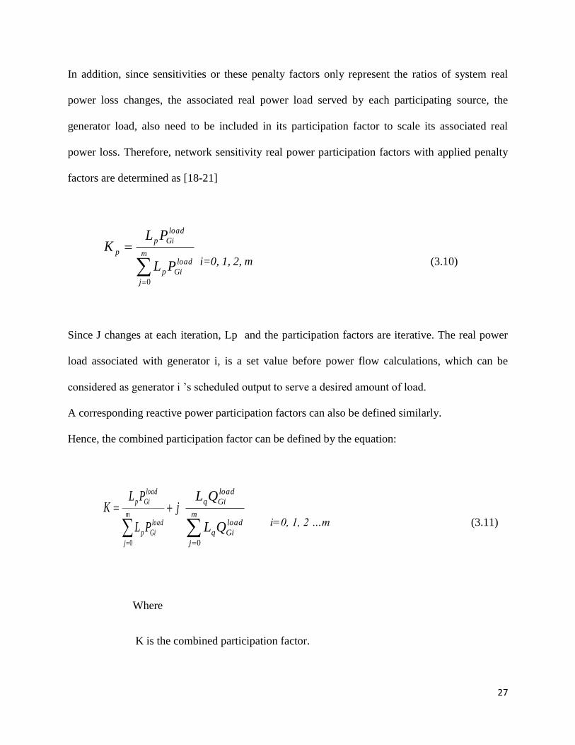
In addition, since sensitivities or these penalty factors only represent the ratios of system real
power loss changes, the associated real power load served by each participating source, the
generator load, also need to be included in its participation factor to scale its associated real
power loss. Therefore, network sensitivity real power participation factors with applied penalty
factors are determined as [18-21]
load
Gi
m
j
p
load
Gip
p
PL
PLK
0
i=0, 1, 2, m (3.10)
Since J changes at each iteration, Lp and the participation factors are iterative. The real power
load associated with generator i, is a set value before power flow calculations, which can be
considered as generator i ’s scheduled output to serve a desired amount of load.
A corresponding reactive power participation factors can also be defined similarly.
Hence, the combined participation factor can be defined by the equation:
j
PL
PLK
load
Gi
m
j
p
load
Gip
0
load
Gi
m
j
q
load
Giq
QL
QL
0
i=0, 1, 2 …m (3.11)
Where
K is the combined participation factor.

28
3.2.6 DFIG Domains Combined Participation Factors
The concept of generator domains and commons originates from a transmission system approach
in [18-21]. Each generator’s contribution to loads and losses can be distinguished using generator
domains and commons. Generator domains and commons were determined by post processing a
power flow solution or from available system measurements.
This thesis will adapt the transmission based concepts of generator domains and commons to the
DFIG based distribution systems. Since the loads and network are unbalanced in distribution
systems, the buses and branch flows supplied by the same source may be different across phases.
Thus, to emphasize and clarify individual phases to capture unbalanced situations encountered in
distribution systems, generator domains will be extended to multi-phase DFIG domains in this
thesis.
The concept of multi-phase generator domains strives to distinguish the loss and load associated
with each participating source. As such, an associated loss with each participating source can be
quantified. The effects of network parameters, load distributions and generator capacities are
explicitly included in these participation factors. The generator domain participation factors are
defined by equation (3.1)
In the distributed slack bus model with DFIG the real and reactive power outputs of participating
generators are iterative. DFIG domains and loss contributions vary with changing source
injections. Thus, the participation factors are iterative during power flow calculations. The
process for determining three-phase generator domains presented in [21] will be applied to the
DFIG.

29
3.2.7 Applications of Participation Factors in present work
Participation factors have been applied to assign the system loss to multiple generators during
power flow calculations. In previous works, these participation factors are constant values and
can be determined by different methods. The participation factors are related to the
characteristics of turbines on each generator bus and load allocation, combined cost and
reliability criteria in power flow for fair pricing and scheduled generator outputs. The
participation factors are also applied to minimize active power generation using the nonlinear
version of the Interior Point Method (IPM).
With increasing interest on reactive power dispatch and control in distribution systems, reactive
power control for DGs also has become possible [22, 23].The amount of reactive reserves at
generating stations is a measure of the degree of voltage stability. With this perspective, an
optimized reactive reserve management scheme based on the optimal power flow presented in
[24] show that detailed models of generator limiters, such as those for armature and field current
limiting must be considered in order to utilize the maximum reactive power capability of
generators, so as to meet reactive power demands during voltage emergencies. Participation
factors for each generator in the management scheme are predetermined based on the V-Q curve
methodology and the results prove that the proposed method can improve both static and
dynamic voltage stability.
Optimization Algorithms for reactive power have been presented in [25] by exact loss formula,
in [26] by PSO and by GA in [27] .In [28, 29], the management of reactive power generation to
improve the voltage stability margin using modal analysis technique is done and the simulation
results show that after the optimal reactive power re-scheduling, the active/reactive power losses
are decreased. All these optimization methods provide no means of distributing the slack to
30
various DGs in the power system for a distributed generation scenario with intermittent
renewable and uncertain loads.
Pushpendra Singh, L S Titare and L D Arya, 2013 [17] developed a DE-based algorithm
optimizes a set of reactive power control variables and maximizes reactive reserve available at
generating buses using generation participation factors. Voltage dependent reactive power limits
have been accounted. The optimal settings of reactive power control variables have been
obtained for next interval predicted loading condition. These optimized settings satisfy the
operating inequality constraints in predicted load condition as well as in present base case
loading conditions. Obtained results using DE have been compared with those obtained using
another population based techniques PSO and CAPSO.
3.2 Single Slack Bus Model
The traditional power flow analysis identifies the slack bus as the reference for the voltage angles
of all buses and the power-balancing bus that makes up for the difference between the scheduled
generation and the combined loads and losses. Hence, the slack bus is considered a voltage
source with a large power capacity [18-21].While this model is viable for the utility connected
operation ,where the utility bus can be assumed as an“infinite power source “with respect to the
DER units, it exhibits severe limitations for the islanded ADN. The slack bus in an islanded
ADN is essentially a grid-forming (PV bus) DER unit whose generation capacity is comparable
to the other operating DERunits.If the reference bus output power ,i.e., the slack, exceeds its
DER unit nominal capacity, it becomes essential to distribute the system slack among other
participating units, based on a pre-specified criterion. The single slack bus (SSB) model does not
allow for slack distribution analysis since it assigns all the system slack to one bus.

31
3.3 Distributed Slack Bus Model
In balanced transmission systems, distributed slack buses were introduced to remedy the
inadequacy of a single slack bus.[18-21].The concept of DSB-based power-flow analysis for
balanced transmission networks [30]–[31] and unbalanced distribution grids [18]–[21] has been
addressed in the technical literature.
Several criteria have been developed to distribute the slack among the participating sources
including constant participation factors based on the source scheduled output [21],[30-31] ,
iteratively calculated participation factors based on the source domains and commons [18]–[21]
and iteratively calculated participation factors based on the real power network sensitivity and
penalty factors for real power .
The existing three-phase DSB models are incorporated in phase-frame power-flow algorithms,
which are less computationally efficient than their sequence-frame counterparts [32], [33]. In
addition, deploying these models permit the grid-forming DG units (PV buses) to share only the
system real slack. Such a practice is not the best option for an islanded ADN where the DG fleet
may consist of power-controlled (PQ) DG units, intermittent renewable and varying loads.
In addition, distributing the reactive slack for the DFIGs has not yet been addressed in the
technical literature[32,34] .This research thesis also demonstrates that distributing the reactive
slack can significantly reduce the reference bus output, and thus prevent its power capacity limit
violation. As such, the main contribution of this work is introducing a DSB model that can
efficiently deal with unbalanced three-phase networks, distribute the reactive slack, and
incorporate the PQ controlled DG units in the real and reactive slack sharing through the
combined participation factors.
32
3.3.1 DFIG Based Distributed Slack Bus Model
Although the voltage and current unbalance in a distribution Grid could be significant, the power
unbalance (which is defined as the ratio of the negative-plus the zero-sequence power
components to the positive-sequence power component) is much smaller. Thus, it is reasonable
to assume that the total system three-phase power slack is approximately three times its positive-
sequence counterpart. Hence, the DFIG based distributed slack bus model in this thesis is defined
based on the positive-sequence powerflow, and is incorporated with the positive-sequence
power-how equations [32] where the bulk of the power system slack is associated with.
Based on the adopted control strategy, a DFIG unit can be categorized as a grid-forming
(voltage-controlled) unit that dictates the voltage and a power-controlled (PQ) unit that
exchanges pre-specified real and reactive power with the system [32]. The latter can be further
divided, based on the DFIG capacity, into a large or a small PQ unit. To formulate the
Distributed Slack Bus model, the DFIG units that participate in compensating the System slack
must be predetermined. The participating units are classified as [32].
PV and large PQ units with spare real power capacity to compensate for the system real
slack. The ratio of the real slack contribution of each participating unit to the total system
real slack is the “real-power participation factor” as in equation (3.1).
Large PQ units with spare reactive power capacity to compensate for the system reactive
slack. The “reactive-power participation factor,” is defined as the ratio of the reactive
slack contribution of each participating unit to the total system reactive slack as in
equation (3.2).

33
3.4 Solution Algorithm for Reactive Power Participation Factors
The real power participation factors developed in [18-21] for the general distributed
generator will be applied for the DFIG Real power and thus in this section only the reactive
power distributed slack model for the Newton Raphson(NR) method is developed to
distribute the reactive slack .The Newton Raphson(NR) method choice for the distributed
slack bus model in this thesis since ,as compared to the Gauss Siedel method(GS),NR has the
following merits[5,7]:
Its rate of convergence is fast and therefore requires less number of iterations to obtain
the solution.
It is independent of the number of buses of the system hence it can be applied on large
practical systems.
The convergence of the method is not affected by the selection of the slack bus; hence
there is freedom of distributing the slack bus.
It is more accurate and reliable when used for large systems.
A general comparison of NR with other load flow study methods is as shown in the Table 3.1

34
Table 3.1 Comparison of load flow methods for new distribution networks [1, 5, 7]
A Newton Rapson Solver Incorporating the distributed slack model with iterative participation
factors is used .This algorithm works for both network sensitivity and DFIG domain
participation factors. The steps for the algorithm are as follows:
Step 1: Choose an initial guess at 𝑥(0)
Step 2: Set the iteration counter at 𝑘 = 0

35
Step 3: Set desired 𝑄𝐺𝑖𝑙𝑜𝑎𝑑 𝑎𝑛𝑑 𝑖𝑛𝑖𝑡𝑖𝑎𝑙 𝐾𝑞
Step 4: Evaluate 𝐹(𝐾)(𝑋(𝐾))
Step 5: Stop if |𝐹(𝐾)| ≤ 𝑇𝑜𝑙𝑒𝑟𝑎𝑛𝑐𝑒
Step 6: Evaluate Je(k)
=∂F
∂x
Step 7: Solve 𝐽𝑒(𝑘)
∆𝑥(𝑘) = −𝐹(𝑘)
Step 8: Let 𝑥(𝑘+1) = 𝑥(𝑘) + ∆𝑥(𝑘)
Step 9: Let 𝑘 = 𝑘 + 1
Step 10: Check real and reactive power limits of the participating DFIGs.If the calculated
real/reactive power output of a DFIG violated its limits, this DFIGs cannot be considered as a
participating source which accounts for slack and is modelled as a constant PQ injection
Then go to Step 3
Step 11: Upgrade calculation information. For sensitivity participation factors, calculate
sensitivities and for generator domain participation factors, find positive power flow directions
and distinguish generator domains for the substation and participating DFIGs.
Step 12: Calculate reactive power participation factors 𝐾𝑞(𝑘)
𝑎𝑛𝑑 𝐾0(𝐾)
,and go to Step 4.
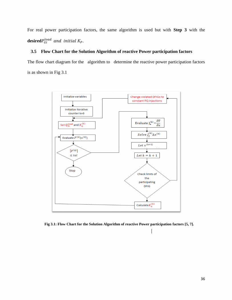
36
For real power participation factors, the same algorithm is used but with Step 3 with the
desired𝑃𝐺𝑖𝑙𝑜𝑎𝑑 𝑎𝑛𝑑 𝑖𝑛𝑖𝑡𝑖𝑎𝑙 𝐾𝑃.
3.5 Flow Chart for the Solution Algorithm of reactive Power participation factors
The flow chart diagram for the algorithm to determine the reactive power participation factors
is as shown in Fig 3.1
Fig 3.1: Flow Chart for the Solution Algorithm of reactive Power participation factors [5, 7].

37
3.6 Simulation Results and Analysis
The results presented in this section include those of the effects of combined participation factors
on power loss and voltage profile plus the effected of the proposed DSB the power losses and
voltage profile.
3.7.1 Participation factors and Power loss
Simulation results including the real and reactive power participation factors, real and reactive
power outputs obtained using the different slack bus models of the 33 bus radial distribution
system are as shown in the Table 3.1 and Table 3.2 below for cases 1 and case 2 respectively.
From these numerical simulation results, the impacts of different slack bus models for distributed
generation with DFIGs were observed. For the single slack bus model, both cases keep the
DFIGs at the same output out 1.5MW and 750KVAR.The combined participation factors is 1,
that of the substation.
The distributed slack bus model with non-iterative participation factors based on scheduled
DFIG capacity alone has the same real and reactive participation factors values in both cases.
Thus, with the same DFIG output, the amount of the output attributed to loads compared to the
system losses are the same even though the DFIG is located at different locations. The combined
participation factor is better than the corresponding real and reactive factors. Since this method
does not capture the effects of DFIG locations on power system studies, it is not recommended.
However it is better than the single slack bus model.
The distributed slack bus model with sensitivity participation factors were computed in two
ways; based on average sensitivities and maximum phase sensitivities. The resulting real reactive
and combined participation factors were slightly different between these two methods. It is noted

38
that both methods assigned larger participation factors to the DFIG on Bus 18than when the
DFIG was placed on Bus 19. Thus the sensitivity and penalty factor approach performed, as
expected, with respect to attributing higher losses to the DFIG at bus 18, the primary distribution
system. . The sensitivity measures are significant enough to fully capture the effects of DFIG
locations by assigning real reactive and combined participation factors to the respective DFIGs.
DFIG domains DSB does not capture the economic aspects of the network and also the details
of all network parameters. However this method confirms the optimal place for the slack bus is
the primary distribution system at high losses
The following key is used to interpret the results in tables 3.1 and 3.2
A-Single slack Bus Model [5, 7, 20]
B-Distributed Slack bus model based on DFIG capacity [36]
C-Distributed Slack bus model based on average sensitivity [This method]
D-Distributed Slack bus model based on maximum sensitivity [[This method]
E-Distributed Slack bus model based on DFIG domain [17, 21]
Unlike the existing DSB models, the proposed formulation the DFIG based DSB Simultaneously
distributes both real and reactive slack by the application of the combined participation factors.
From Table 3.1 and 3.2, the magnitude of the combined participation factor is greater than the
individual real and reactive participation factors, hence a better strategy to distribute the slack.
Also this model Involves DFIG units, with control strategies for the reactive power so as to
compensate the total slack hence an alternative way to control the voltage profile. In addition,
this DSB model guarantees the power flow solution to adhere with the DFIG operating limits.

39
Case A
Table 3.1:33 Bus Radial Distribution System with DFIG on Bus 18 to Service 1500KW 750KVAR Load
A[5,7,20] B[36] C[This
Method ]
D[This
Method]
E[17,21 ]
Sub Par KO 1 0.7515 0.7468 0.7497 0.6749
DFIG par
KP=18
0 0.2485 0.2532 0.2503 0.3251
DFIG par
Kq=18
0 0.2356 0.2448 0.2709 0.3099
Com.K 1 0.3424 0.3552 0.3688 0.4492
Ø(deg) 0 43.47 44.03 47.26 43.63
𝑃𝑠𝑢𝑏𝑜𝑢𝑡 (𝑀𝑊) 475.052 470.554 470.554 471.554 468.593
𝑃𝐷𝐹𝐼𝐺𝑜𝑢𝑡 (𝐾𝑊) 1.5000 1.5232 1.5232 1.5232 1.5629
𝑄𝐷𝐹𝐼𝐺𝑜𝑢𝑡 (𝐾𝑉𝐴𝑅) 750.0000 750.0083 750.0128 750.0156 750.0165
𝑃𝑙𝑜𝑠𝑠𝑠𝑦𝑠
(𝐾𝑊) 221.4340 221.4238 221.4238 221.4238 220.4225
𝑄𝑙𝑜𝑠𝑠𝑠𝑦𝑠
(𝐾𝑉𝐴𝑅) 150.1784 150.1780 150.1776 150.1770 150.1765

40
Case B:
TABLE 3.2:33 Bus Radial Distribution System with DFIG on Bus 19 to Service 1500KW 750KVAR Load
A[5,7,20] B[36] C[This
method]
D[This
method]
E[17,21 ]
Sub. Par KO 1 0.7515 0.7633 0.7555 0.9866
DFIG par
Kp=19
0 0.2485 0.2367 0.2445 0.0134
DFIG par
Kq=19
0 0.2296 0.2295 0.2386 0.0108
Comb.K 1 0.3384 0.3297 0.3416 0.0172
Ø(deg) 0 42.74 44.12 44.30 38.87
𝑃𝑠𝑢𝑏𝑜𝑢𝑡 (𝑀𝑊) 476.1162 471.6651 471.6651 471.6651 476.2040
𝑃𝐷𝐹𝐼𝐺𝑜𝑢𝑡 (𝐾𝑊) 1.5000 1.5265 1.5565 1.5565 1.5012
𝑄𝐷𝐹𝐼𝐺𝑜𝑢𝑡 (𝐾𝑉𝐴𝑅) 750.0000 750.0083 750.0128 750.0156 750.0165
𝑃𝑙𝑜𝑠𝑠𝑠𝑦𝑠
(𝐾𝑊) 221.4340 221.4344 221.4340 221.4341 220.9992
𝑄𝑙𝑜𝑠𝑠𝑠𝑦𝑠
(𝐾𝑉𝐴𝑅) 150.1784 150.1780 150.1776 150.1770 150.1765
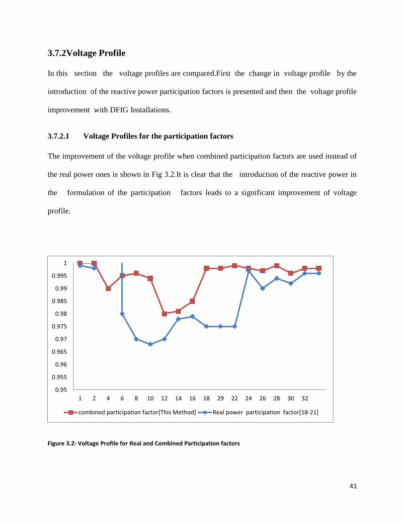
41
3.7.2Voltage Profile
In this section the voltage profiles are compared.First the change in voltage profile by the
introduction of the reactive power participation factors is presented and then the voltage profile
improvement with DFIG Installations.
3.7.2.1 Voltage Profiles for the participation factors
The improvement of the voltage profile when combined participation factors are used instead of
the real power ones is shown in Fig 3.2.It is clear that the introduction of the reactive power in
the formulation of the participation factors leads to a significant improvement of voltage
profile.
Figure 3.2: Voltage Profile for Real and Combined Participation factors
0.95
0.955
0.96
0.965
0.97
0.975
0.98
0.985
0.99
0.995
1
1 2 4 6 8 10 12 14 16 18 29 22 24 26 28 30 32
combined participation factor[This Method] Real power participation factor[18-21]
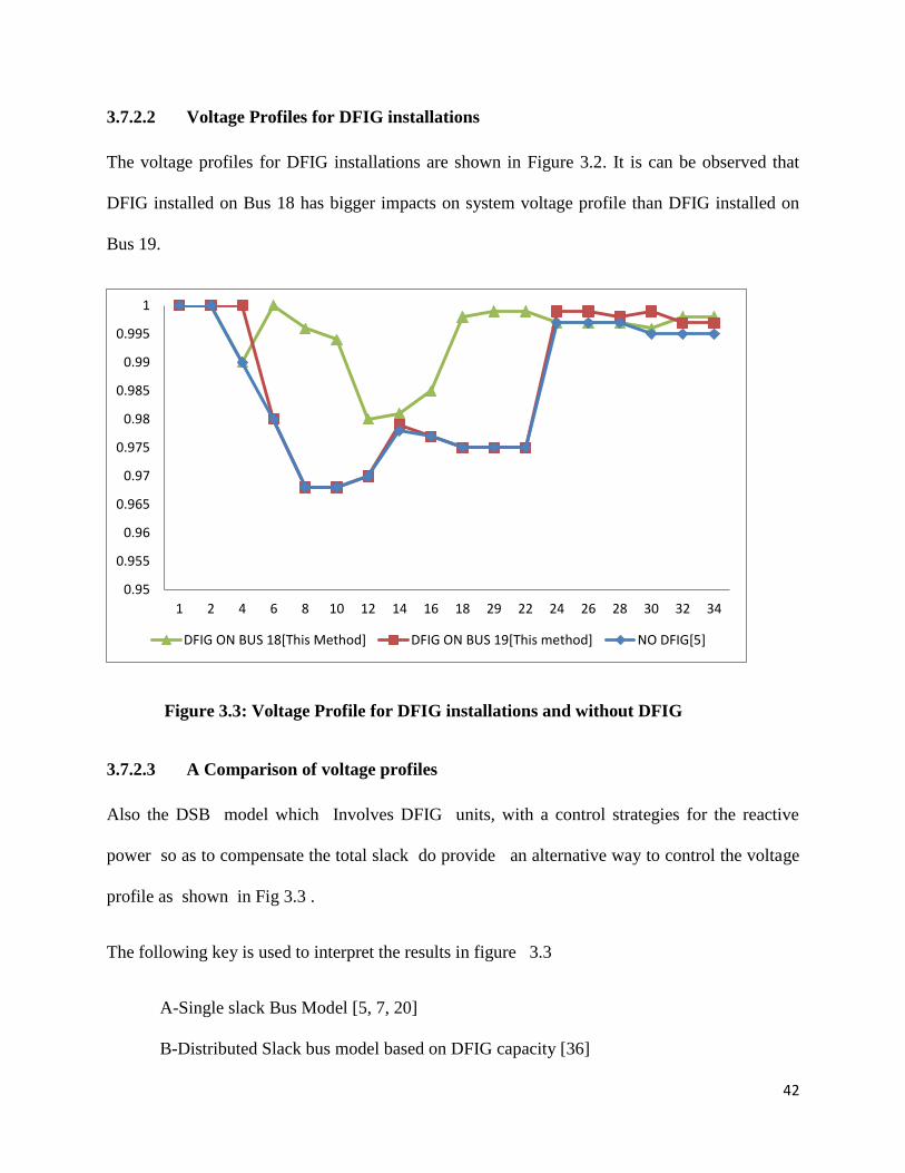
42
3.7.2.2 Voltage Profiles for DFIG installations
The voltage profiles for DFIG installations are shown in Figure 3.2. It is can be observed that
DFIG installed on Bus 18 has bigger impacts on system voltage profile than DFIG installed on
Bus 19.
Figure 3.3: Voltage Profile for DFIG installations and without DFIG
3.7.2.3 A Comparison of voltage profiles
Also the DSB model which Involves DFIG units, with a control strategies for the reactive
power so as to compensate the total slack do provide an alternative way to control the voltage
profile as shown in Fig 3.3 .
The following key is used to interpret the results in figure 3.3
A-Single slack Bus Model [5, 7, 20]
B-Distributed Slack bus model based on DFIG capacity [36]
0.95
0.955
0.96
0.965
0.97
0.975
0.98
0.985
0.99
0.995
1
1 2 4 6 8 10 12 14 16 18 29 22 24 26 28 30 32 34
DFIG ON BUS 18[This Method] DFIG ON BUS 19[This method] NO DFIG[5]
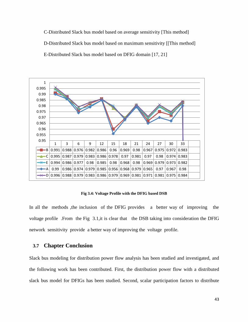
43
C-Distributed Slack bus model based on average sensitivity [This method]
D-Distributed Slack bus model based on maximum sensitivity [[This method]
E-Distributed Slack bus model based on DFIG domain [17, 21]
Fig 3.4: Voltage Profile with the DFIG based DSB
In all the methods ,the inclusion of the DFIG provides a better way of improving the
voltage profile .From the Fig 3.1,it is clear that the DSB taking into consideration the DFIG
network sensitivity provide a better way of improving the voltage profile.
3.7 Chapter Conclusion
Slack bus modeling for distribution power flow analysis has been studied and investigated, and
the following work has been contributed. First, the distribution power flow with a distributed
slack bus model for DFIGs has been studied. Second, scalar participation factors to distribute
1 3 6 9 12 15 18 21 24 27 30 33
B 0.991 0.988 0.976 0.982 0.986 0.96 0.969 0.98 0.967 0.975 0.972 0.983
C 0.995 0.987 0.979 0.983 0.986 0.978 0.97 0.981 0.97 0.98 0.974 0.983
E 0.994 0.986 0.977 0.98 0.985 0.98 0.968 0.98 0.969 0.979 0.973 0.982
A 0.99 0.986 0.974 0.979 0.985 0.956 0.968 0.979 0.965 0.97 0.967 0.98
D 0.996 0.988 0.979 0.983 0.986 0.979 0.969 0.981 0.971 0.981 0.975 0.984
0.95
0.955
0.96
0.965
0.97
0.975
0.98
0.985
0.99
0.995
1
44
uncertain real and reactive power system losses for three phase power flow calculations have
been formulated using network sensitive combined participation factors. Also two methods to
calculate network-based participation factors have been presented; sensitivity-based method and
generator domain based method. Lastly a GA based NR solver implemented the distributed
slack model with iterative combined participation factors.
The distribution power flow with a single slack bus model was revisited, and a distributed slack
bus model was developed for distribution systems with DFIGs. The combined participation
factors based on generator network sensitivity, which are explicitly relative to network
parameters and load distributions, demonstrate their ability to capture network characteristics and
to scale loss contributions of sources surpasses other combined participation factors. Therefore,
the DFIG based distributed slack model with network sensitive combined participation factors
is recommended for the allocation of real and reactive power losses to various buses.
The studies also conclude that simultaneous distribution of real and reactive slack positively
impacts the operation of the ADN by reducing the real power losses, and improving the voltage
profile, thus increasing the system overall efficiency.

45
Chapter 4
DFIG PLACEMENT AND SIZING
In this chapter, the DFIG placement and sizing problem is solved using an hybrid of GA and
PSO (HGAPSO) and the results compared with those obtained by doing the placement using
load flow and ordinary PSO.An overview of DG placement and sizing is given .
4.1 DG Placement and Sizing
S .Tong, 2006 [18-21] carried out a study on DG placement and sizing. Rau and Wan have used
gradient and second order method to minimize loss ,line loading and reactive power
requirements in the Distribution network .Willis investigated loss minimization using analytical
based 2/3 rule ,assuming a constant power source and a uniformly distributed load.
Hybrid and Constraint Based Multi Objective Programming(HCBMOP) and GA method was
proposed by Celli et al to minimize the cost of network upgrading ,power losses and energy
required by customer. He later used the method to minimize the cost of network upgrading
,cost of energy losses and DG network acceptability index with the DG fully considered as a
valid planning alternative.GA and Multiple Attribute Making Decision (MAMD) approach has
been used on a PQ model DG to investigate its technical attributes such as reactive power
flows, voltage variation and active loss as well as the economic attributes which include line
congestion ,capital cost and emission.
An Heuristic Iterative Search method was also used to minimize the cost of investment
and operation of DGs,loss and energy required by customers, which was later applied to
minimize DG investment and operation losses and energy purchased from the main grid.

46
Anti- Colony Optimization (ACO) was applied on a time varying load to minimize investment
cost, operation cost and energy buying from transmission grid. Further Particle Swarm
Optimization was used on a multi- load level to minimize the cost of active losses,
investment and operation cost of DG and emission cost.
The other methods used in the DG placement and sizing so far include analytical approach
simulated annealing optimal power flow ,sensitivity analysis, fast sequential quadratic
programming and NSGA II and max-min approach .
All these methods are limited in that they have not taken into consideration the reactive power
losses which can no longer be ignored due to their increased importance in maintaining the
voltage profile. Again such methods have not taken care of the intermittent renewable which
today are forming a significant part of the active distribution network.
4.2 DFIG Placement and Sizing
With wind taken into consideration , a GA with decision making approach was used by
Carpinelli et al,2001,[37] to minimize the cost of power losses and network upgrading for a
general wind generator with a peak load and constant load growth.
Ochoa el al,2008,[38] used multi objective optimization with NSGA for a wind turbine
generator with a time varying load to maximize the integration of DG and energy export
;minimizing losses and short circuit level.
These two methods have not considered the placement of the DFIG with an objective of
optimizing the real and reactive losses. For the first time, the placement and sizing of the

47
commercial DFIG is considered in this chapter using a hybrid of GA and PSO (HGAPSO) and
its effects on the real power losses and the reactive power losses and the voltage profile studied.
Juanuwattanakul et al, 2012, [39] proposed an effective method for placement of DFIG units in
multiphase distribution networks based on system voltage profile using PSO. The approach
consists of utilizing the positive sequence voltage ratio V collapse/Vno-load to identify the weakest
three-phase bus for the installation of DFIG units. DFIG ratings are determined by evaluating
their impacts on voltage profile, grid losses and maximum loading factor while considering the
voltage limits at all buses. The impacts of DIFG on voltage profile, active power loss and voltage
stability margin are highlighted. The PSO approach developed in this work is used for
comparison with HGAPSO method developed in this chapter.
4.3 The DFIG Capability Limit Curves
The model of a DFIG used in this thesis consists of a pitch controlled wind turbine and an
induction generator[36,40].The stator of the DFIG is directly connected to the grid ,while the
rotor is connected to the converter consisting of two back to back pulse width modulated
(PWM) inveters,which allow direct control of the rotor currents.
Direct control of the rotor currents allows for the variable speed operation and reactive power
control thus the DFIG can operate at a higher efficiency over a wide range of wind speeds and
thus help in providing voltage support for the power grid.
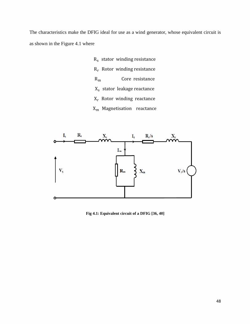
48
The characteristics make the DFIG ideal for use as a wind generator, whose equivalent circuit is
as shown in the Figure 4.1 where
Rs stator winding resistance
Rr Rotor winding resistance
Rm Core resistance
Xs stator leakage reactance
Xr Rotor winding reactance
Xm Magnetisation reactance
Fig 4.1: Equivalent circuit of a DFIG [36, 40]

49
The stator active and reactive power can be expressed in terms of the stator and rotor currents as
in the equations 4.2 and 4.3[36, 40],
(4.2)
(4.3)
Where
Ps is the real stator power
Qs is the reactive stator power
In the PQ plane, the equation (4.1) represents the circumference centered at the origin [0, 0] with
the radius equal to the stator speed apparent power. Equation (4.2) represents a circumference
centered at [−3𝑉𝑆2 𝑋𝑆,0]⁄ and radius equal to [3(𝑋𝑚𝑉𝑆𝐼𝑟) 𝑋𝑆,]⁄ .Therefore given the maximum
rotor and stator allowable currents limits ,𝐼𝑟 𝑚𝑎𝑥 and 𝐼𝑆 𝑚𝑎𝑥 , the DFIG capability limits can
be obtained.The composed DFIG capability limits curve is shown in Figure 4.2 where
𝑈𝑆 is used instead of 𝑉𝑆 . Taking the steady state stability of the DFIG into account,
represented by the vertical line at the [−3𝑉𝑆2 𝑋𝑆,, 0]⁄ cordinate,it is obvious that the DFIG real
and reactive power capability mainly depends on the maximum allowable rotor current.
)3(222
IVQP rsss
.
2
)3()3(
22
2
IVX
X
X
VQP rs
s
m
s
ssS

50
From the Figure 4.2, the DFIG can operate at any point in the intersecting area within the given
limits. When the available active power is far from its maximum, the amount of reactive power is
high. The large reactive power control capabilities of the DFIG make it possible to use DFIG as
the continuous reactive power support to support system voltage control.
Figure 4. 2: DFIG Capability limits curve [40]
4.4 Problem Formulation
The real power loss in the distribution system is very significant from the system operation point
of view. The difference between the generated power and the power demand gives the power
loss.

51
That is:
(4.3)
Where
Is the total real power loss
Is the generated power
Is the power demand
The objective of the placement technique is to minimize the total real power loss.
Mathematically, the objective function can be written as:
(4.4)
n
ilossL PP
1
n
iDFIGiP
1
n
iDiP
1
n
iL
n
iDi
n
iPPPDFIGi
111
VVR
K
VVR
K
QPPQKQQPPKP
Pp
ji
jiij
t
ji
jiij
i
jijitjiji
n
i
n
jiL
n
ilossL
where
with
)sin(
)cos(
).()(
min
1 1
1
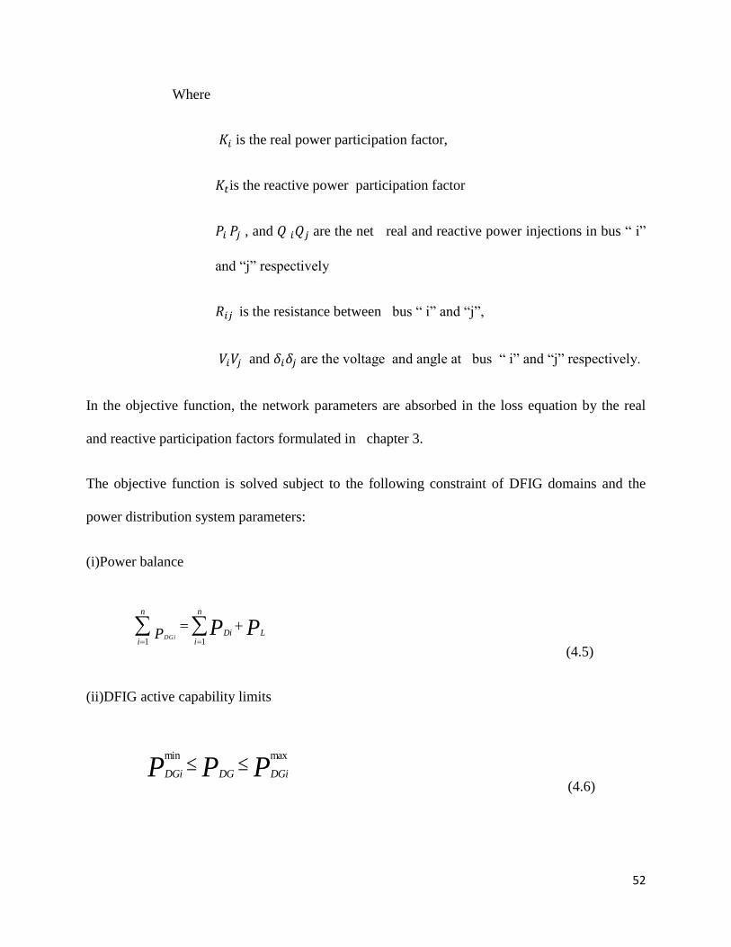
52
Where
𝐾𝑖 is the real power participation factor,
𝐾𝑡is the reactive power participation factor
𝑃𝑖 𝑃𝑗 , and 𝑄 𝑖𝑄𝑗 are the net real and reactive power injections in bus “ i”
and “j” respectively
𝑅𝑖𝑗 is the resistance between bus “ i” and “j”,
𝑉𝑖𝑉𝑗 and 𝛿𝑖𝛿𝑗 are the voltage and angle at bus “ i” and “j” respectively.
In the objective function, the network parameters are absorbed in the loss equation by the real
and reactive participation factors formulated in chapter 3.
The objective function is solved subject to the following constraint of DFIG domains and the
power distribution system parameters:
(i)Power balance
(4.5)
(ii)DFIG active capability limits
(4.6)
PP L
n
iDi
n
iPDGi
11
PPP DGiDGDGi
maxmin

53
(iii)DFIG reactive capability limits
From
(4.7)
Since for the DFIG, 𝑋𝑚 ≫≫ 𝑋𝑠 the middle term for the product of the reactive power
component can be ignored hence,
(4.8)
(4.9)
Where
PDFIGi is the real power generated by DFIG i
QDFIGi is the reactive power generated by DFIG i
(v)Voltage constraints at the buses
(4.10)
)3()3(
22
2
2
IVX
X
X
VQP rs
s
m
s
sDFIGiDFIGi
)3)32
((
2
2
2
2
X
VPIV
X
XQ
s
srs
s
mDFIGiDFIGi
.
2
(( )3)3
2
2
2
2
X
VPIV
X
XQ
s
srs
s
mDFIGiDFIGi
VVV iii
maxmin

54
(vi)Line thermal limit
(4.11)
4.5 HGAPSO Method
HGAPSO is made up of two pure optimization methods GA and PSO.The individual methods
are discussed and then the hybrid formed is presented.
4.5.1 Particle Swarm Optimization (PSO)
Swarm Intelligence (SI) is an innovative distributed intelligent paradigm for solving optimization
problems that originally took its inspiration from the biological examples by swarming, flocking
and herding phenomena in vertebrates[12] Particle Swarm Optimization (PSO) incorporates
swarming behaviors observed in flocks of birds, schools of fish, or swarms of bees, and even
human social behavior, from which the idea is emerged .PSO is a population-based optimization
tool, which could be implemented and applied easily to solve various function optimization
problems. As an algorithm, the main strength of PSO is its fast convergence, which compares
favorably with many global optimization algorithms like Genetic Algorithms (GA) Simulated
Annealing (SA) and other global optimization algorithms. For applying PSO successfully, one of
the key issues is finding how to map the problem solution into the PSO particle, which directly
affects its feasibility and performance [20].
4.5.2 Genetic Algorithm (GA)
Genetic Algorithms are a family of computational models inspired by evolution. These
algorithms encode a potential solution to a specific problem on a simple chromosome-like data
PP ijij
max
55
structure and apply recombination and mutation operators to these structures so as to preserve
critical information[12].An implementation of a genetic algorithm begins with a population of
(usually random) chromosomes.
One then evaluates these structures and allocates reproductive opportunities in such a way that
those chromosomes which represent a better solution to the target problem are given more
chances to reproduce than those chromosomes which are poorer solutions. The goodness of a
solution is typically defined with respect to the current population.
The genetic algorithm can be viewed as two stage process. It starts with the current population.
Selection is applied to the current population to create an intermediate population. Then
recombination and mutation are applied to the intermediate population to create the next
population. The process of going from the current population to the next population constitutes
one generation in the execution construction of the intermediate population is complete and
recombination can occur. This can be viewed as creating the next population from the
intermediate population. Crossover is applied to randomly paired strings with a probability
denoted Pc. A pair of strings is picked with probability Pc for recombination. These strings form
two new strings that are inserted into the next population. After recombination, mutation
operator is applied. For each bit in the population, is mutated with some low probability Pm.
Typically the mutation rate is applied with less than 1% probability. In some cases mutation is
interpreted as randomly generating a new bit in which case, only 50% of the time will the
mutation actually change the bit value. After the process of selection, recombination and
mutation, the next population can be evaluated. The process of evaluation, selection,
recombination and mutation forms one generation in the execution of a genetic algorithm.

56
4.5.3 Hybrid of PSO and GA (HGAPSO)
The drawback of PSO is that the swarm may prematurely converge [12]. The underlying
principle behind this problem is that, for the global best PSO, particles converge to a single
point, which is on the line between the global best and the personal best positions. This point is
not guaranteed for a local optimum .Another reason for this problem is the fast rate of
information flow between particles, resulting in the creation of similar particles with a loss in
diversity that increases the possibility of being trapped in local optima.
A further drawback is that stochastic approaches have problem-dependent performance. This
dependency usually results from the parameter settings in each algorithm. The different
parameter settings for a stochastic search algorithm result in high performance variances. In
general, no single parameter setting can be applied to all problems. Increasing the inertia weight
(w) will increase the speed of the particles resulting in more exploration (global search) and less
exploitation (local search) or on the other hand, reducing the inertia weight will decrease the
speed of the particles resulting in more exploitation and less exploration. Thus finding the best
value for the parameter is not an easy task and it may differ from one problem to another.
Therefore, from the above, it can be concluded that the PSO performance is problem-dependent.
The problem-dependent performance can be addressed through hybrid mechanism. It combines
different approaches to be benefited from the advantages of each approach.
To overcome the limitations of PSO, hybrid algorithms with GA are proposed. The basis behind
this is that such a hybrid approach is expected to have merits of PSO with those of GA. One
advantage of PSO over GA is its algorithmic simplicity. Another clear difference between PSO
and GA is the ability to control convergence. Crossover and mutation rates can subtly affect the
convergence of GA, but these cannot be analogous to the level of control achieved through

57
manipulating of the inertia weight. In fact, the decrease of inertia weight dramatically increases
the swarm’s convergence. The main problem with PSO is that it prematurely converges to stable
point, which is not necessarily maximum. To prevent the occurrence, position update of the
global best particles is changed. The position update is done through some hybrid mechanism of
GA. The idea behind GA is due to its genetic operators crossover and mutation. By applying
crossover operation, information can be swapped between two particles to have the ability to fly
to the new search area. The purpose of applying mutation to PSO is to increase the diversity of
the population and the ability to have the PSO to avoid the local maxima.
There are three different hybrid approaches are proposed. In PSO-GA (Type 1), the gbest particle
position does not change its position over some designated time steps, the crossover operation is
performed on gbest particle with chromosome of GA. In this model both PSO and GA are run in
parallel.
In PSO-GA (Type 2), the stagnated pbest particles are change their positions by mutation
operator of GA. Lastly, in PSO-GA (Type 3), the initial population of PSO is assigned by
solution of GA. The total numbers of iterations are equally shared by GA and PSO. First half of
the iterations are run by GA and the solutions are given as initial population of PSO. Remaining
iterations are run by PSO
In this thesis, the PSO-GA type 2 is preferred since we are interested in changing the siting of the
DFIGs optimizes the power losses, taking their capacities as a constant.
PSO, which is stochastic in nature and makes use of the memory of each particles as well as the
knowledge gained by the swarm as a whole, has been proved to be powerful in solving many
optimization problems. The hybrid PSO systems find a better solution without trapping in local

58
maximum, and to achieve faster convergence rate. This is because when the PSO particles
stagnate, GA diversifies the particle position even though the solution is worse. In PSO-GA,
particle movement uses randomness in its search. Hence, it is a kind of stochastic optimization
algorithm that can search a complicated and uncertain area. This makes PSO-GA more flexible
and robust. Unlike standard PSO, PSO-GA is more reliable in giving better quality solutions with
reasonable computational time, since the hybrid strategy avoids premature convergence of the
search process to local optima and provides better exploration of the search process.
4.6 Proposed HGAPSO Algorithm
The HGAPSO based approach for solving the optimal sizing and placement of the DFIG is
aimed at minimizing the distribution line real and reactive losses. In this thesis, the reactive
power output is obtained by means of the DFIG power curves after the active power output is
known. The total active power output is obtained by the equation(4.5).Considering the
capability limits of the DFIGs,the maximum of the reactive power that each DFIG can generate
or absorb, the HGAPSO based approach for solving the problem to minimizes the losses takes
the following steps.
Step 1: Input the line and bus data and the bus voltage limits
Step 2: calculate the loss using distribution load flow based on backward forward sweep
Step 3: Randomly generate an initial population (array) of particles with random initial positions
and velocities on dimensions in the solution space.Set the iteration counter 𝑘 = 0
Step 4: For each particle, if the bus voltage is within the limits, perform mutation on the particle
position, one by one, keeping the velocity fixed, then perform mutation on the velocity, keeping

59
the position fixed. Other n positions and k velocities are obtained. Calculate the total losses as in
equation 1 in each case.
Step 5: For each particle, compare its objective position and velocity with the individual best .If
the objective value is lower than Pbest, set this value as the current Pbest, and record the
corresponding particle position.
Step 6:Compare all components of the particle according to their fitness values. Choose the
particle associated with the minimum individual best Pbest of all the particles and set the value
of this Pbest as the current overall best Gbest
Step 7: If the iteration number reaches the maximum limit, go to step 9.Otherwise set iteration
index 𝑘 = 𝑘 + 1 and go back to step 4
Step 8: Update the velocity and position of the particle
Step 9: If the particle equals to the population size N, print out the optimal solution of the
targeted problem, otherwise set the particle to i=1 and go to step 3.
Step 10.Assign Combined participation Factors to each particle taking into consideration the
DFIG domains chapter 3
The best position includes the optimal locations and sizes of the DFIGs and the corresponding
fitness value represents the minimum total real power loss.
The flow chart for the proposed HGAPSO algorithm is as shown in the Fig 4.3

60
Figure 4.3 Flow chart for HGAPSO Algorithm
4.7 Results and Analysis
The simulation results presented in this section concern the power loss reduction and the
improved voltage profile.
4.7.1 Power Loss Reduction
Simulations were run on the IEEE 33Bus Radial distribution Test System [35] the real and
reactive power losses obtained through load flow, PSO and HGAPSO are as shown in the Tables
4.1, 4.2 and 4.3
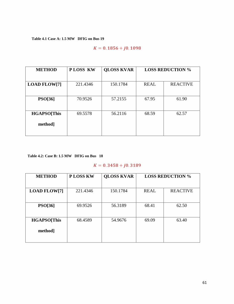
61
Table 4.1 Case A: 1.5 MW DFIG on Bus 19
𝑲 = 𝟎. 𝟏𝟖𝟓𝟔 + 𝒋𝟎. 𝟏𝟎𝟗𝟖
Table 4.2: Case B: 1.5 MW DFIG on Bus 18
𝑲 = 𝟎. 𝟑𝟒𝟓𝟖 + 𝒋𝟎. 𝟑𝟏𝟖𝟗
METHOD P LOSS KW QLOSS KVAR LOSS REDUCTION %
LOAD FLOW[7] 221.4346 150.1784 REAL REACTIVE
PSO[36] 69.9526 56.3189 68.41 62.50
HGAPSO[This
method]
68.4589 54.9676 69.09 63.40
METHOD P LOSS KW QLOSS KVAR LOSS REDUCTION %
LOAD FLOW[7] 221.4346 150.1784 REAL REACTIVE
PSO[36] 70.9526 57.2155 67.95 61.90
HGAPSO[This
method]
69.5578 56.2116 68.59 62.57

62
Table 4.3: Case C: 1.5 MW DFIG on Bus 3
𝑲 = 𝟎. 𝟎𝟐𝟑𝟒 + 𝒋𝟎. 𝟎𝟏𝟖𝟕
METHOD P LOSS KW QLOSS KVAR LOSS REDUCTION %
LOAD FLOW[7] 221.4346 150.1784 REAL REACTIVE
PSO[36] 68.8536 53.8907 68.91 64.12
HGAPSO[This
method]
66.5578 50.8765 69.94 66.12
The load flow method determines the total real and reactive power losses accurately in the 33 bus
radial distribution system. The basic PSO seems to provide better loss reduction than the load
flow but this is not accurate enough since the PSO algorithm may have converged before all
the buses are considered.
The HGAPSO on the other hand provides a better loss reduction technique compared to the PSO
in that the mutation operator ensures no local /premature convergence occur and thus it can be
applied in practical distribution systems. The % real and reactive power loss reduction is better
with HGAPSO as compared to the load flow and the PSO.
4.7.2 Bus Voltage Profile
The voltage level of all the buses keep the standards level of voltages (+-5%) with load flow,
PSO and HGAPSO as shown in the Fig 4.5 .However, the voltage is more improved by using
HGAPSO

63
Fig 4.4: Bus Voltages Profile after DFIG Placement using PSO and HGAPSO and load flow
4.8 Chapter Conclusion
The DFIG wind turbines are capable of reducing both real and reactive power losses in a power
distribution system; however they need to be placed at suitable locations. The PSO algorithm is
optimally placing the DFIG with the objective of reducing the total real power losses in the
primary distribution systems. The PSO is fast and accurate in determining the sizes and the
locations. However this ordinary PSO is prone to local minima and premature convergence
hence not applicable in solving real life power system optimization problems.
The HGAPSO algorithm performs the optimisation over a larger search space since it escapes
from local minima and increases the diversity of variable values using the mutation operator. The
HGAPSO optimises in a better way, the real and reactive power losses at the same time giving an
improved voltage profile.
The numerical results shows that the integration of the DFIG wind turbines into the traditional
power distribution system is highly effective in reducing real and reactive power losses in the
0 5 10 15 20 25 30 35
0.978
0.98
0.982
0.984
0.986
0.988
0.99
0.992
0.994
0.996
0.998
0.965
0.97
0.975
0.98
0.985
0.99
0.995
1
1 3 6 13 28 30
PSO[36] LOAD FLOW[7] HGAPSO[This Method]

64
primary distribution System9 buses 18 and 3 in this case ) when HGAPSO is used as compared
to the ordinary PSO.
In DFIG placement and sizing with the objective of optimizing real and reactive power
losses ,the bus to which the DFIG domain Distributed Slack Bus Model assigns a large
Combined Participation Factor is considered as the optimal site for the DFIG.In this case the
large combined participation factor is assigned to DFIG In bus 3 and 18 ,the primary
distribution system .
When well applied to a DFIG, the HGAPSO can be used to reduce the real and reactive power
losses by 70% and 67% at the same time giving an improvement of the voltage profile by almost
0.3% from the PSO and by almost 0.6% from the load flow.
From the tabulated results, the best locations corresponding to the optimum size for reducing the
total real and reactive power losses is in the primary distribution system.

65
Chapter 5
ACTIVE DISTRIBUTION NETWORK RECONFIGURATION
(ADNR) PROBLEM WITH WIND & UNCERTAIN LOAD
This chapter deals with the active distribution network reconfiguration (ADNR) problem taking
into consideration wind based DFIG and uncertain loads. A hybrid of bacterial foraging (BF) and
Differential evolution (DE) (HBFDE) is formulated and then applied for a stochastic wind
scenario and the results compared with those of a deterministic case. First, an introduction to
network configuration is given in the next section.
5.1 Background
The configuration of most electric distribution networks is radial for proper protection
coordination. Due to some objectives such as supply all of the loads, reduce power loss, increase
system security and enhancement of power quality, the configuration of these networks may be
changed with automatic or manual switching operations. Distribution network reconfiguration
also relieves the overloading of network components. This change is performed by opening
sectionalizing (normally closed) and closing tie (normally open) switches of the network. These
switching operations are performed in such a way that all of the loads are energized and the
radiality of the network is preserved.
From the impact of DG on power distribution networks, the distribution system reconfiguration
is found to have more line losses and reduced terminal voltage as compared to transmission
network. For optimizing power loss, the new reconfiguration is used as the feeder
reconfiguration systematic method to operate the distribution system at minimum cost and with
66
improved system reliability and security. By opening or closing the feeder switches, load
currents can be transferred from feeder to feeder thus helping to study the effect of DG on the
distribution networks with reference to network reconfiguration problems. The combination of
feeder reconfiguration and DG placement process not only reduce the power loss but also
improve the voltage profile. DGs are not only employed to provide real and /or reactive power
compensation in distribution systems but also to reduce the power losses and to maintain the
voltage profile within the acceptable limits. In this thesis the wind based DFIG has been be
considered.
The numerous advantages of the DFIG in terms of their low or zero emission and their much
smaller size than conventional central power plants have created more incentives than before to
use these kinds of generators with free energy source. Therefore, it is necessary to study the
impact of DFIGs units on the distribution networks especially on the ADNR [41]-[42].
5.2 Network Reconfiguration Review
The problem of NR is not a new one. Many studies have undertaken the challenge of loss
minimization in the area of the network reconfiguration. One of the first researches on this area
had been introduced by Merlin and Back, 1975, [43]. They solved the problem by the branch
and bound method. But the introduced method has two drawbacks. Firstly, the convergence of
the solution was not guaranteed, and secondly it required a huge amount of calculations for a real
network.
R.J. Sarfi et al ,1994 [44], proposed a simple innovative method for calculating loss through the
network reconfiguration, which is based on some simplifications in order to calculate the change
of loss in load transfer from one feeder to another. Later Awaji and Galiana, 2012[45]
67
improved the method proposed in [44] with a few corrections. The main drawbacks of the
method are that there is no guarantee to reach the global solution and the final solution depends
on the initial status of the tie and sectionalizing switches.
Due to the evolution of the central grid into a smart one the studies and approaches to NR have
changed significantly. Many recent researchers have used evolutionary algorithms to solve
ADNR problem in [46, 47], a problem for loss reduction and load balancing as an artificial bee
colony (ABC) problem was modeled. Qiwang et al, 2009, [48] introduced a power-flow-
minimum heuristic algorithm for ADNR problem. In [49], a model based automated strategy
was considered the ADNR problem taking the smart grid into consideration. J. Torres-Jimenez
et al, 2010 [50] proposed a GA and Spanning trees multi-objective approach to solve the ADNR
problem [50]. In [51], an algorithm was considered for efficient and automatic NR based on the
service restoration and load balancing in a real-time operation. The method was based on
differential evolution (DE). Chiou et al, 2005, [52] presented a variable scaling hybrid
differential evolution (VSHDE) to solve the ADNR. In his work, minimizing the power loss was
considered as the objective function. Nuno and Susana, 2011 [53] proposed a method for
network reconfiguration to minimize power loss by using the improved MIHDE.In [54], a PSO
based algorithm for multi-objective ADNR with fault restoration is proposed. Wu et al, 1989,
[55] proposed a hybrid algorithm based on GA and PSO for ADNR problem while Yu et al,
2009, [56] proposed an improved genetic algorithm with infeasible solution disposing for the
ADNR problem.
In all mentioned work, the ADNR problem has been solved without considering the DFIG and
the stochastic wind scenario. In general the challenges facing the integration of Wind energy into
the grid have been ignored.
68
5.3 ADNR with Wind Based DFIG
The most recent studies on the ADNR problem with wind has been done by considering general
wind turbines. To achieve the reconfiguration of distribution network with wind turbine, Shuang
et al, 2012 [57], raised a probability-based scenario analysis to form typical scenarios of wind
turbine with consideration of statistical characteristics of wind energy output. By generating the
switch-state graph of distribution system, NR was simplified to the optimization problem of
network switch-state combination. For model solution, a genetic algorithm (GA) and the way of
"breaking circle" was employed to seek optimal network reconfiguration scheme with wind
turbine under mono-scenario and the multiscenario.
Zhou et al, 2011 [58] proposed a chance constrained programming formulation for distribution
reconfiguration with WTG that aims at minimum power loss and increasing voltage quality. A
scenario analysis method was applied to describe the random output of WTG through the
scenario probability and scenario output. A multiple objective PSO (MOPSO) was employed to
solve the multi-objective discrete nonlinear optimization problem. The dedicated particle
encoding with the mesh information of the distribution network can effectively avoid producing
a large amount of invalid solutions. With MOPSO, it was possible to obtain the optimum
solution set of each objective while helping the operator to choose the most appropriate plan for
reconfiguration.
Yuqing et al, 2010, [59] presented a novel scenario distribution network reconfiguration model
in which the scenario analysis method was applied to describe the random output of the WTG
and its influence through the scenario selection and scenario voltage. Multiple WTGs and wind

69
farms connected with a network was also considered in this model. An efficient GA was
presented for the scenario distribution network reconfiguration model. Through the non-feasible
coding rule in the initial population strategy, cross strategy and eugenic strategy, individuals in
the evolution always form the feasible solutions which can meet the requirement of the actual
distribution network. Physical optimization based on scenario voltage in the process of evolution
reduces the optimization time and the dependence of the initial population. All these studies are
based on general WTGs and are therefore not suitable for the commercial DFIG.In Addition the
hybrid optimization methods are the state of the art means for a real time and real world power
system for they enhance the strengths of the methods involved and discard their weaknesses.
Jingjing Zhao et al, 2009, [60] proposed a joint optimization algorithm of combining reactive
power control of wind farm with DFIG and network reconfiguration. In the proposed joint
optimization algorithm, an improved hybrid particle swarm optimization with wavelet mutation
algorithm (HPSOWM) was developed for voltage profile improvement which utilized reactive
power output of wind farm as the control variable. In each particle updating instance at each
iteration of reactive power output optimization algorithm, a binary particle swarm optimization
algorithm (BPSO) is utilized to find the optimal network structure. This problem will be revisited
in this thesis by using an HBFDE algorithm
In the distribution system, due to many candidate switching combinations and also presence of
DFIG units, the ADNR problem is modeled as a MINLP problem. Various methods such as LP,
MIP, QP, can be used to solve this problem. However, in many cases, the classical methods fail
to provide the global optimum solution and only reach local solution.

70
In recent years, the BF and DE algorithms have been proposed as two powerful optimization
evolutionary algorithms in the field of optimization [61]-[62]. Although in many cases, BF
eventually determines the desired solution, its convergence rate is slow and its local search is
weak. In other side, DE algorithm has a good performance in the local search area but its global
search is weak and its performance depends on the proper selection of the initial population. In
this thesis, a hybrid method is employed to combine the BF and DE algorithms (HBFDE) based
on the evolutionary natures of them. This will take the advantage of the compensatory property
of both of them and avoid their negative points. Most important advantage of proposed HBFDE
algorithm is high accuracy in finding the optimal switching combination of the distribution
system to minimize the network loss.
In addition, the decision maker must be able to balance the consumption and generation of
energy at both short and long time intervals. Due to intermittent nature of wind and loads, this is
difficult for the network operator to balance the consumption and production of energy when the
wind turbines are feeding the electrical network [63]-[65]. This is the main reason why a good
prediction has a significant role in the handling of the DFIG and loads in electrical networks.
Hence, in this thesis, the system uncertainty including the DFIGs and loads are modelled in a
stochastic approach based on scenarios. The scenarios are generated using the roulette wheel
mechanism which models the stochastic behaviours of the wind speed and loads uncertainty.
Moreover, an aggregation method is used to decrease the computation burden and extract one
scenario among all generated scenario so that the uncertainty of all scenarios are considered in
aggregated scenario based on their probability. Finally, the HBFDE algorithm is used to optimize
the problem for deterministic and stochastic (aggregated) scenarios.

71
5.4 ADNR Problem Formulation with Wind
The ADNR problem considering the DFIG is a mixed integer nonlinear optimization problem.
(MINOP). In this problem, there are many different objective functions including loss
minimization, balancing the load on transformers, balancing the load on feeders, maximum
loading of feeders and minimizing the deviation of voltages from nominal value. In this thesis,
power loss minimization is considered as the objective of ADNR problem with regard to DFIG,
while the other objectives are considered as constraints. The minimization of total real power
loss is calculated as follows [63]:
2
1
(X)brN
i i
i
f R I
tie1 2 1 2 1 2 1 (2 )X [ , ,..., , , ,...., , , ,..., ]tie tieWTG WTGi N N N N NTie Tie Tie Sw Sw Sw pf pf pf
Where ,
iR resistance of the ith branch
iI actual current of the ith branch
tieN number of tie switches
WTGN number of WTG units, in this case DFIG
(5.1)
The vector X has three sections: iTie , that represents the situation of tie switches in ith loop and
get ‘0’ and ‘1’ values corresponding to open and close states, respectively. Indeed, if the iTie is
0, it means that the tie switch of ith loop must remain unchanged (open), also if it is ‘1’ , it means

72
that tie switch of ith loop must be closed .The iSw that is one of the sectionalizing switches in ith
loop, replace the tie switch of that loop. The third part of vector X is the power factor of ith
DFIG.
The constraints of the proposed problem are expressed as follows [63, 64]:
Distribution line limits,
Line
ij
Line
ij PP max,
where
LineijP
power flowing over distribution lines
This constraint defines the power security of the system
(5.2)
Distribution power flow equations,
)sin(YVVQ
)cos(YVVP
jiijijj
N
1i
ii
jiijijj
N
1i
ii
bus
bus
Where
iP net injected active power components at the ith bus.
iQ net injected reactive power components at the ith bus.
(5.3)

73
iV amplitude of voltage at the ith bus
i angle of voltage at the ith bus
The radiality of the network,
1 busbrFL NNN
Where
FLN number of main loops
busN number of buses
brN number of branches
In this thesis, the main closed loops of the system are used to
check the radial structure of the network
(5.4)
Limit on the currents of the transformers,
titit NiII ,...,2,1max
,,
(5.5)

74
Where
itI , current amplitude of the ith transformer
tN number of transformers
The current limit of the feeders,
fifif NiII ,...,2,1max
,,
Where
ifI , current amplitude of the ith feeder
fN number of feeders
(5.6)
Active power constraints of the DFIG,
min, , , max, ,w i w i w ip p p
Where
,w ip Generated active power of ith DFIG.
(5.7)

75
Bus voltage amplitudes ,
min maxiV V V (5.8)
Power factor constraints of the DFIG,
iii pfpfpf max,min, (5.9)
5.5 The Stochastic Model of DFIG and Loads
In this case, there is need to balance the consumption and production of energy in a system
considering DFIG. Hence we must make a good prediction of wind speed and loads. In this
thesis, to make a good prediction of uncertainty parameters, the wind and loads uncertainty are
considered based on the wind and loads forecast error [64, 65]. So, the probability distribution
function (PDF) of the wind and loads forecast error should be constructed .In this thesis a typical
PDF has been considered. The continuous distribution function of the wind forecast error along
with its discretization is shown in Fig.5.1 according to which seven intervals are centered on the
zero mean and each of intervals are one wind speed forecast error standard deviation, as
presented in [66]. Finally, a roulette wheel mechanism [67] is implemented to generate scenarios
for the proposed time. In the roulette wheel mechanism, scenarios are selected on the basis of
different wind and loads forecast levels and their probabilities obtained from the PDF.

76
Wind error
Pro
bab
ilit
y d
ensi
ty
Win
d lev
el 7
Win
d lev
el 5
Win
d lev
el 6
Win
d lev
el 4
Win
d lev
el 3
Win
d lev
el 2
Win
d lev
el 13
6
4
7
5
2
Fig 5.1: Discretization of PDF of wind forecast error
For this purpose, at first, the probabilities of different wind and loads forecast levels are
normalized such that their summation becomes equal to unity. Then, by roulette wheel
mechanism a scenario is obtained. In this regards, as shown in Fig. 5.2, the range of 0-1 is
occupied by the normalized probabilities. After that, random numbers are generated between 0
and 1. Each random number falls in the normalized probability range in the roulette wheel .The
selected interval is associated with a binary digit equal to 1, and other interval becomes zero.
Wind le
vel 1
Wind level 2Wind level 3
Wind level 4
Wind level 5 Win
d lev
el 6
Win
d lev
el 7
Roulette
wheel
0-1
Fig 5.2: Roulette Wheel Selection

77
After obtaining the wind and load forecast level for all DFIGs and loads, a scenario
corresponding to all DFIGs and loads is produced. A scenario is a vector of binary parameters
that identify the wind and loads intervals: This procedure is repeated until the desired number of
scenarios is generated by the relation [64]
1 1 1 1 1 17, 7, 7, 7,1, 1, 1, 1, 1 (7( ))[ , ... , ,..., , ... , , , ... , ,..., , ... , ]
WTG loadn
WTG WTG WTGn WTGn load load loadn loadnn n n nn n n n N Nscenario W W W W W W W W
(5.10a)
The probability of all scenarios is then calculated by equation 5.10b [64]
(5.10)
Where
,jWTG
i nW binary parameter indicating whether the ith wind interval of ith WTG is
selected in the ith scenario.
senN Number of scenario
nscenarioP Probability of the nth scenario
α is the coefficient of power of WTG j in the nth scenario of the wind forecast
error, standard deviation which is a measure of uncertainty of wind loading.
7 7
, , , , , , , ,
1 11 1
7 7
, , , , , , , ,
1 1 11 1
. . .
( . . . )
1,2,...
WTG load
n WTG loadsen
N N
WTG load
n i j n i j n r m n r m
i rj m
Senario N NNWTG load
n i j n i j n r m n r m
k i rj m
sen
w w
p
w w
n N

78
Finally, obtained wind speed is converted to the active power of DFIGs according to the
equation [68]:
1 3
1 2
2 3
0 ,
( )
w w
w w w
n w
v v v v
P v v v v
p v v v
(5.11)
Where,
v1, v2 and v3 are, cut in, rated and cut-out wind speeds respectively (m/s)
𝑃𝑤 the output power from a wind turbine
𝛷(𝑉𝑤)Power generated between the cut in and rated speed which is a
function of the wind speed
𝑃𝑛 power generated between rated and cut out speeds
𝑉𝑤 The useful wind speed (m/s)
5.6 The HBFDE Algorithm
HBFDE algorithm consists of two pure optimization methods, BF and DE.In this section the pure
methods and the proposed hybrid is presented. We begin with an overview of the pure
methods.

79
5.6.1 Bacterial Foraging (BF) Algorithm
The Bacterial Foraging algorithm (BF) has been implemented in the global optimization field
in the recent years. BF algorithm is based on the foraging behaviour of the E. coli bacteria. Each
bacterium by its selection behaviour tries to eliminate the poor foraging strategy and modifies the
successful foraging strategy. As the other evolutionary algorithms, this algorithm is designed to
solve non-gradient optimization problems with non-differentiable and complex objective
functions such as DNR problem. In BF algorithm, each possible solution is considered as
bacteria. There are three main steps in the original BF algorithm, namely; chemotaxis,
reproduction and elimination or dispersal [61].
The initial population of bacteria must be produced in their search space according to the
equation,
1
1 2 1 2
1 2
( ) (2 )
1 (2 )
X
.
_ .
.
X
,
X [ , ,..., , , ,....,
, , ,..., ] , 1, 2,...,
BF
tie
tieBF WTG
tie
tieWTG WTG
N
i N N
BF
N N N
N N N
BF Population
for
Tie Tie Tie Sw Sw Sw
pf pf pf i N
(5.12)
The chemotaxis step is composed of a set of consequence swimming following by tumble. At
first, based on the rotation of the flagella, the bacterium selects the direction that it should move
(tumbling). Then, if the new position of bacterium is better than previous, the bacteria will begin
to move in the same previous direction (swimming). A unit length in a random direction
represents a tumble; ( )j , this random direction specifies the direction of the movement after

80
a tumble. The constant run-length unit, ( , )C i j , determines the size of the step taken in the
random direction. In the proposed algorithm, the location of the ith bacterium at the jth
chemotactic step, kth reproduction step and lth elimination/dispersal event is represented by
( , , )i j k l ,and the objective function is shown by ( , , , )J i j k l . After a tumble the location of ith
bacteria is shown by the equation,
( 1, , ) ( , , ) ( , ) ( )i ij k l j k l C i j j (5.13)
If the obtained objective function at ( 1, , )i j k l is better (lower) than ( , 1, , )J i j k l , another step
of size ( , )C i j in the same direction is taken. This swimming operation is repeated as long as a
lower objective function is obtained until a maximum present number of steps are reached.
The objective function of each bacterium in the population is affected by swarming, that is
performed by the cell-to-cell signalling released by the bacteria groups to form swarm patterns.
This procedure is expressed as follows [62]:
1
2
1 1 1 1
( , ( , , )) ( , ( , , ))
[ exp( ( ))] [ exp( ( ) )]
si i
cc cc
i
p ps si i
attract attract m m repellant repellant m m
i m i m
J P j k l J j k l
d w h w
(5.14)
Where, attractd , attractw , repelllanth and repellantw are coefficients representing the characteristics of
the attractant and repellent signals released by the cell and i
m is the mth component of ith
bacteria position i .

81
Also, the position of each member of the population of the S bacteria is show by ( , , )p j k l and
defined as:
( , , ) ( , , ) 1,2,...ip j k l j k l i s
(5.15)
Where
S is the size of the bacteria population.
( , ( , , ))ccJ P j k l represents the cell-to-cell signaling effect, is added to the ( , , , )J i j k l .
After cN steps of chemotactic, the reproduction process is performed. In this step, the population
is halved so that the least healthy half dies and each bacterium in the other healthiest one splits
into two bacteria that take the same position.
2r
SS
An elimination/dispersal process is performed after taking a maximum number of chemotactic
steps,reN . In this operation each bacterium could be moved to the new position of the search
space
5.6.2 Differential Evolutionary (DE) Algorithm
The Differential Evolutionary (DE) algorithm was proposed by Ji-PyngChiou et al [52] and
futher studied and implemented by D.Pal et al ,[51] .This algorithm is a very simple and
straightforward optimization strategy .The main concept of DE is conducted by means of four
main operations: 1-initialization, 2-mutation, 3- crossover, 4- selection.
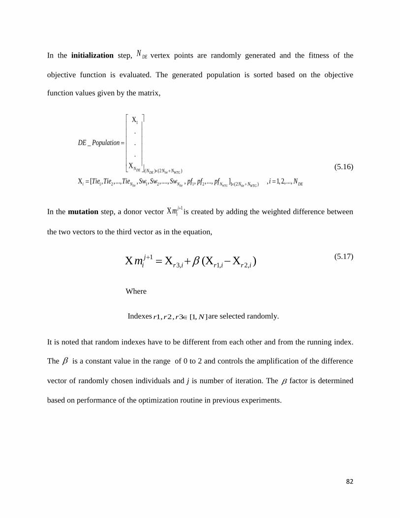
82
In the initialization step, DEN vertex points are randomly generated and the fitness of the
objective function is evaluated. The generated population is sorted based on the objective
function values given by the matrix,
1
1 2 1 2 1 2
( ) (2 )
1 (2 )
X
.
_ .
.
X
X [ , ,..., , , ,...., , , ,..., ] , 1,2,...,WTG
DEtieDE WTG
tie tie tie WTG
N
i N N N DE
N N N
N N
DE Population
Tie Tie Tie Sw Sw Sw pf pf pf i N
(5.16)
In the mutation step, a donor vector 1X j
im is created by adding the weighted difference between
the two vectors to the third vector as in the equation,
1
3, 1, 2,X X (X X )j
i r i r i r im (5.17)
Where
Indexes ],1[3,2,1 Nrrr are selected randomly.
It is noted that random indexes have to be different from each other and from the running index.
The is a constant value in the range of 0 to 2 and controls the amplification of the difference
vector of randomly chosen individuals and j is number of iteration. The factor is determined
based on performance of the optimization routine in previous experiments.
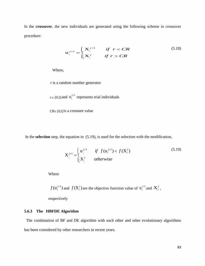
83
In the crossover, the new individuals are generated using the following scheme in crossover
procedure:
1
1X
uX
i
i
i
j
j
j
if r CR
if r CR
(5.18)
Where,
r is a random number generator
]1,0[r and 1u j
i
represents trial individuals
]1,0[CR is a constant value
In the selection step, the equation in (5.19), is used for the selection with the modification,
1 1
1u (u ) (X )
XX
i
i
i
j j j
i ij
j
if f f
otherwise
(5.19)
Where
1(u )j
if and (X )j
if are the objective function value of 1u j
i
and X
j
i ,
respectively
5.6.3 The HBFDE Algorithm
The combination of BF and DE algorithm with each other and other evolutionary algorithms
has been considered by other researchers in recent years.

84
In [42] and [69], BF and DE has been combined to perform economic load dispatch with non-
convex loads and improve the performance of algorithms by increasing the effect of swarming.
In [52], a variable scaling hybrid DE algorithm has been proposed to dominate the problem of
the selection of a mutation operator. But, this thesis aims at the integration of BF and DE
algorithms, to combine their advantages and avoid their negative points. For example, DE
algorithm is a very efficient local search procedure, but it is not always available since it is very
sensitive to the choice of the initial condition and there is no guarantee to obtain the global
optimization. Also, the accuracy of the BF algorithm is not very high and its local search is
weak. But, by combining these algorithms, the new algorithm namely, HBFDE algorithm has a
better convergence rate in comparison to original BF and DE algorithms.The proposed algorithm
works for all Wind Turbine Generators (WTG)
5.7 The ADNR Algorithm with Wind and Load Uncertainty
The algorithm consists of two major sections which are outlined in the sections 5.7.1 and
5.7.2.First the DFIG scenarios are generated and then the HBFDE algorithm is formulated.
5.7.1 The algorithm for the DFIG scenario generation
Step 1: Set i as the initial number of trials; i=i+1
Step 2: Import the basic information; that is the bus and load data.
Step 3: Generate 1000 scenarios for the DFIGs speed.
Step 4: Determine the aggregate of the 1000 generated scenarios using equation (5.10).
Step 5: Use equation (5.11) to determine the DFIG output.

85
5.7.2 The HBFDE Algorithm Mechanism
Step 6: Generate the initial population.
Step7: Let J be the number of HBFDE iterations, J=J+1.
Step 8: Evaluate the objective function for initial population; that is the power loss.
Step 9: Sort the initial population based on augmented objective function value.
Step 10: Devide the sorted population to BF and DE algorithms. The population size is
set at 3N, when solving an N-dimensional problem. The initial 3N solutions are randomly
generated and sorted by their fitness, and the top N=NDE solutions fed into the DE
method to improve their positions. The other 2N=NBF solutions are updated by the BF
method. In the BF algorithm N neighborhood of bacterium is proposed to expand the
local search area. The neighbourhoods best bacterium are selected by first evenly
dividing the 2N bacterium into N neighbourhoods and designating the bacterium with the
better fitness value in each neighbourhood as the neighbourhood’s representative. After
first iteration of BF and DE, the first combination is completed. In the second
combination, the 3N updated solutions are sorted again for repeating the entire run. This
process is performed after taking a maximum number of combinations.
Step 11: Combine the updated population from step 10 to generate the HBFDE
population
Step 12: Compare the HBFDE iterations J and the initial number of trials i. If J<Jmax then
update the HBFDE iterations to J=J+1 and go back to Step 7 .Otherwise go to Step 13.
Step 13. If i˃imax then output results, otherwise go back to Step 1.
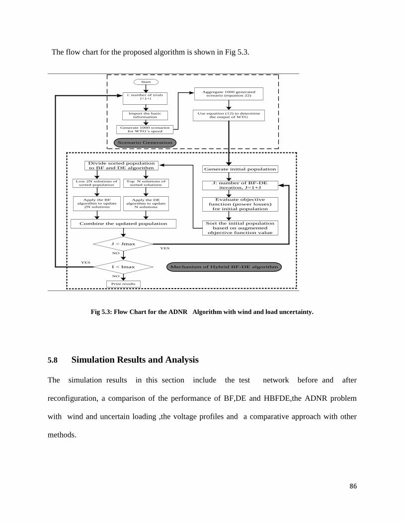
86
The flow chart for the proposed algorithm is shown in Fig 5.3.
Start
Import the basic
information
Generate 1000 scenarios
for WTG’s speed
Aggregate 1000 generated
scenario (equation 22)
Generate initial population
Apply the DE
algorithm to update
N solutions
Apply the BF
algorithm to update
2N solutions
Top N solutions of
sorted solutions
Low 2N solutions of
sorted population
Divide sorted population
to BF and DE algorithm
Sort the initial population
based on augmented
objective function value
Evaluate objective
function (power losses)
for initial population
J: number of BF-DE
iteration, J=1+J
Use equation (12) to determine
the output of WTG
Combine the updated population
J < Jmax
I < Imax
NO
YES
YES
NO
Mechanism of Hybrid BF-DE algorithm
Scenario Generation
Print results
i: number of trials
i=1+i
Fig 5.3: Flow Chart for the ADNR Algorithm with wind and load uncertainty.
5.8 Simulation Results and Analysis
The simulation results in this section include the test network before and after
reconfiguration, a comparison of the performance of BF,DE and HBFDE,the ADNR problem
with wind and uncertain loading ,the voltage profiles and a comparative approach with other
methods.
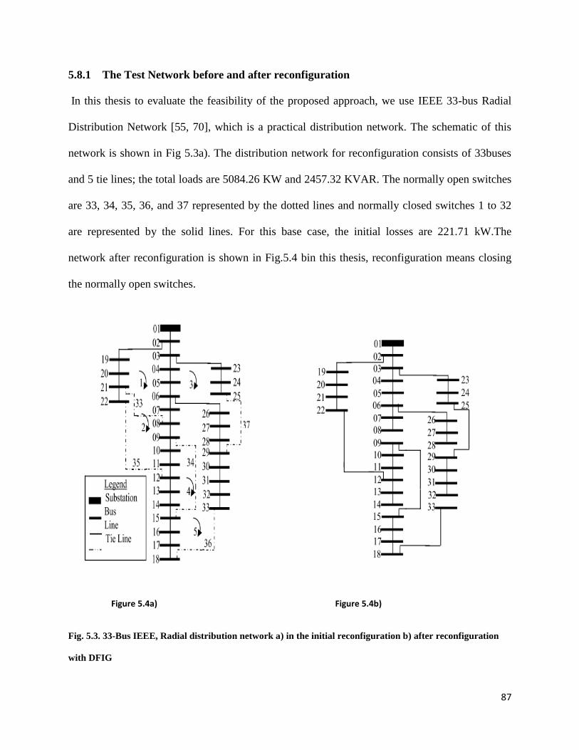
87
5.8.1 The Test Network before and after reconfiguration
In this thesis to evaluate the feasibility of the proposed approach, we use IEEE 33-bus Radial
Distribution Network [55, 70], which is a practical distribution network. The schematic of this
network is shown in Fig 5.3a). The distribution network for reconfiguration consists of 33buses
and 5 tie lines; the total loads are 5084.26 KW and 2457.32 KVAR. The normally open switches
are 33, 34, 35, 36, and 37 represented by the dotted lines and normally closed switches 1 to 32
are represented by the solid lines. For this base case, the initial losses are 221.71 kW.The
network after reconfiguration is shown in Fig.5.4 bin this thesis, reconfiguration means closing
the normally open switches.
Figure 5.4a) Figure 5.4b)
Fig. 5.3. 33-Bus IEEE, Radial distribution network a) in the initial reconfiguration b) after reconfiguration
with DFIG
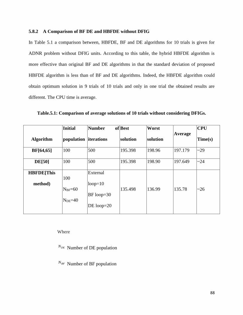
88
5.8.2 A Comparison of BF DE and HBFDE without DFIG
In Table 5.1 a comparison between, HBFDE, BF and DE algorithms for 10 trials is given for
ADNR problem without DFIG units. According to this table, the hybrid HBFDE algorithm is
more effective than original BF and DE algorithms in that the standard deviation of proposed
HBFDE algorithm is less than of BF and DE algorithms. Indeed, the HBFDE algorithm could
obtain optimum solution in 9 trials of 10 trials and only in one trial the obtained results are
different. The CPU time is average.
Table.5.1: Comparison of average solutions of 10 trials without considering DFIGs.
Algorithm
Initial
population
Number of
iterations
Best
solution
Worst
solution
Average
CPU
Time(s)
BF[64,65] 100 500 195.398 198.96 197.179 ~29
DE[50] 100 500 195.398 198.90 197.649 ~24
HBFDE[This
method)
100
NBF=60
NDE=40
External
loop=10
BF loop=30
DE loop=20
135.498 136.99 135.78 ~26
Where
DEN Number of DE population
BFN Number of BF population
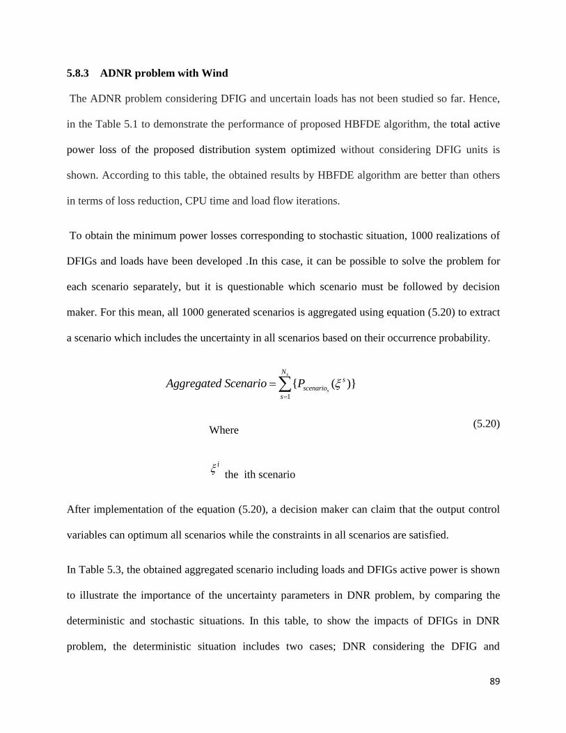
89
5.8.3 ADNR problem with Wind
The ADNR problem considering DFIG and uncertain loads has not been studied so far. Hence,
in the Table 5.1 to demonstrate the performance of proposed HBFDE algorithm, the total active
power loss of the proposed distribution system optimized without considering DFIG units is
shown. According to this table, the obtained results by HBFDE algorithm are better than others
in terms of loss reduction, CPU time and load flow iterations.
To obtain the minimum power losses corresponding to stochastic situation, 1000 realizations of
DFIGs and loads have been developed .In this case, it can be possible to solve the problem for
each scenario separately, but it is questionable which scenario must be followed by decision
maker. For this mean, all 1000 generated scenarios is aggregated using equation (5.20) to extract
a scenario which includes the uncertainty in all scenarios based on their occurrence probability.
1
{ ( )}s
s
Ns
scenario
s
Aggregated Scenario P
Where
i the ith scenario
(5.20)
After implementation of the equation (5.20), a decision maker can claim that the output control
variables can optimum all scenarios while the constraints in all scenarios are satisfied.
In Table 5.3, the obtained aggregated scenario including loads and DFIGs active power is shown
to illustrate the importance of the uncertainty parameters in DNR problem, by comparing the
deterministic and stochastic situations. In this table, to show the impacts of DFIGs in DNR
problem, the deterministic situation includes two cases; DNR considering the DFIG and

90
without considering the impact of DFIGs in network. In last columns of Table 5.3 the optimum
tie switches corresponding to each scenario is shown.
Table.5.2. the Simulation Results for DFIG in Stochastic Scenario
Loss in the base configuration 222.71kw
Loss in the optimal configuration 155.78
Optimal configuration 33,14,8,32,28
Loss reduction 86.93kw
Loss reduction (%) 39.1%
CPU time 0.42 sec
Number of load flow iterations 26
The optimal radial configuration of the IEEE 33 Bus network after all the switching operations is
shown in Figure 5.3b). Table 5.2 shows the simulation results of the base configuration and the
optimal configuration. The minimum and the maximum voltages of the two configurations are
depicted in Fig.5. 4. The power loss before reconfiguration is 222.71 kW and reconfiguration is
155.78 kW. From the results it is observed that reduction in power loss is 86.93 kW which is
approximately 39.1 %. The number of all load flow runs required for the entire process is 26.

91
Table.5.3. The optimum results of deterministic and stochastic situations
Case Power losses [kW] Optimum tie Switches
ADNR considering
DFIG
Stochastic[This Method] 135.89 s34,s14,s8,s32,s28
Deterministic[64,This Method ] 138.97 s35,s14,s8,s32,s28
ADNR without
DFIG
Deterministic[64] 197.398 s37,s14,s8,s32,s28
By comparing the obtained results in Table 5.1 and Table 5.3, it is clear that there are differences
between the results of deterministic and stochastic scenarios. In other side, the probability of the
deterministic scenario is about 4.1% (among 1000 produced scenarios). This means that the
deterministic solution may happen with the low probability of 4.1%. Consequently, the
deterministic scenario cannot be an acceptable solution by itself. On the other hand, using the
obtained aggregated scenario, all 1000 scenarios contribute into determining the ADNR results
according to their probability values. So, the ADNR results of the stochastic framework with
DFIG are more realistic than the deterministic one with DFIG. In other word, the most important
advantage of stochastic scenario is that individual scenario problems become simple to interpret
and with aggregation the 1000 scenarios the underlying problem structure is preserved. Hence
the ADNR problem with wind and uncertain loading is better solved in the stochastic scenario.
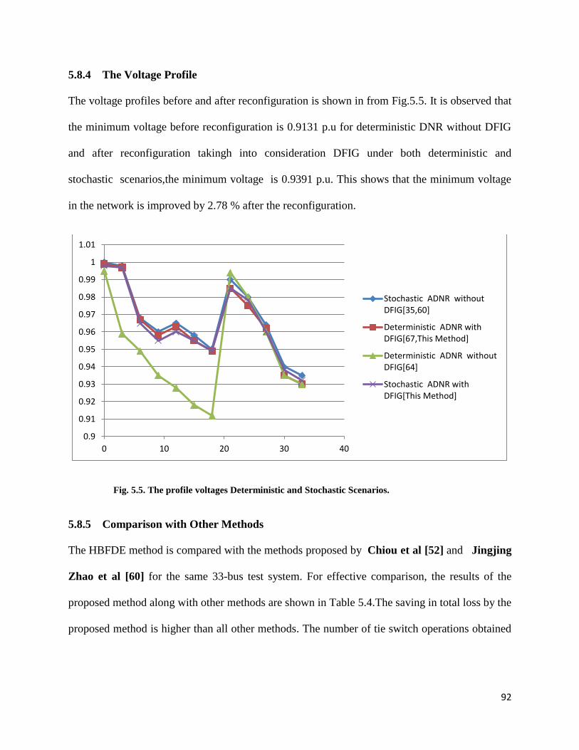
92
5.8.4 The Voltage Profile
The voltage profiles before and after reconfiguration is shown in from Fig.5.5. It is observed that
the minimum voltage before reconfiguration is 0.9131 p.u for deterministic DNR without DFIG
and after reconfiguration takingh into consideration DFIG under both deterministic and
stochastic scenarios,the minimum voltage is 0.9391 p.u. This shows that the minimum voltage
in the network is improved by 2.78 % after the reconfiguration.
Fig. 5.5. The profile voltages Deterministic and Stochastic Scenarios.
5.8.5 Comparison with Other Methods
The HBFDE method is compared with the methods proposed by Chiou et al [52] and Jingjing
Zhao et al [60] for the same 33-bus test system. For effective comparison, the results of the
proposed method along with other methods are shown in Table 5.4.The saving in total loss by the
proposed method is higher than all other methods. The number of tie switch operations obtained
0.9
0.91
0.92
0.93
0.94
0.95
0.96
0.97
0.98
0.99
1
1.01
0 10 20 30 40
Stochastic ADNR withoutDFIG[35,60]
Deterministic ADNR withDFIG[67,This Method]
Deterministic ADNR withoutDFIG[64]
Stochastic ADNR withDFIG[This Method]

93
by the HBFDE and all other methods is 5.The CPU Time for the HBFDE method is the best
compared to the other methods.
Table.5.4.A Comparison of results obtained by optimizing active power loss
Method Final open
switches
Total loss
savings (%)
CPU time
HBFDE[This method ] 33,14,8,32,28 33.1 0.42
Jingjing Zhao et al [60] 7,9,14,32,37 32.6 0.87
Chiou et al [52] 7,9,14,32,37 32.6 1.66
5.9 Chapter Conclusion
In this thesis, a hybrid evolutionary algorithm based on the combination of BF and DE
algorithms called HBFDE has been proposed to obtain the optimal configuration of radial
distribution systems, when the objective function is power loss and holding all the other
objectives of ADNR as constraints. An ADNR has been studied considering the wind based
DFIG. To reach a more realistic solution than the deterministic situation, a stochastic framework
has been considered to model the stochastic behavior of the wind speed and uncertain loads.
Additionally, the simulation results have shown the effectiveness of HBFDE algorithm and the
stochastic approach which can lead to a more efficient utilization of energy in the distribution
systems and permit decision makers to select the possible actions to cope with the wind
uncertainty in the modern power system.

94
Chapter 6
CONTRIBUTIONS AND RECOMMENDATIONS
In this chapter, general thesis conclusions are made, a comparison of the three methods of loss
reduction, contributions of this work, the beneficiaries of the work and finally recommendations
for future work are made.
6.1 General Conclusions
Three methods of power loss reduction in power system with wind wind based distributed
generation has been presented in this work and the following conclusions can be made.
A distributed slack bus model taking into consideration both the DFIG domains and the
network sensitivity using the NR method is the most effective in capturing both real and
reactive power losses. Gauss Siedel (GS) method cannot be applied in formulating the
distributed slack bus since its convergence is affected by the selection of the slack
bus , hence the iterations required to give a solution change with the position of the
slack bus[5,7].
The hybrid methods of power system optimization remain the state of the art methods
for the modern power system with intermittent power.HGAPSO and HBFDE methods
proved effective in power loss reduction and voltage profile improvement as compared
to the pure methods of optimization
The optimal place for power loss reduction is the primary distribution system. The
HGAPSO for DFIG placement and sizing and the DSB with Wind based DFIG Provided
Optimal results in the primary distribution.

95
6.2 Comparison
In this thesis, the distribution test systems used is the IEEE Radial 33 bus systems. The system
has 32 sectionalizing branches, 5 tie switches, nominal voltage of 12.66KV and a total system
load 3.72 MW and 2.3 MVAR. The original total real power loss and reactive power loss in the
system are 221.4346 KW (5.95%) and 150.1784 KNAR (6.53%)
A comparison of the three methods in their effectiveness is as shown in the table 6.1.From the
table it is clear that the DBS is effective in distributing the losses and not reducing them in a
significant way. Also DIG placement is the best in power loss reduction followed by ANDRÉ.
Table 6.1: Comparison of Loss Reduction.
Type of Loss DSB with DFIG DFIG
placement
and sizing
ADNR with Wind
and uncertain loads
Real Losses(KW) 221.4238 69.5578 86.93
% Real Losses 99.99 31.41 60.9
Reactive
losses(KVAR)
150.1770 56.2116 123.338
%Reactive Losses 99.99 37.43 59.7
However the three methods result to an improvement of the voltage profile by 2.96% with the
DFIG based DSB and ADNR with wind being better than the DFIG placement and sizing.

96
Fig 6.1:A comparison of voltage profile improvement.
6.3 Contributions
The technical challenges facing the integration of wind energy into the power grid are of great
concern to the modern power systems designer .Some of these hurdles have been addressed and
the following contributions are made:
Combined participation factors have been formulated, taking into consideration both real
and reactive power losses. These factors have been found more effective in the design of
the distributed slack bus model as compared to the real power participation factors that
existed in the past literature.
A network sensitive distributed slack bus model based on DFIG was designed so as to
distribute real and reactive slacks in the distribution system. A comparison was done with
the single slack bus model, DFIG distributed slack bus model based on DFIG domains
and the DFIG distributed slack bus model based on DFIG capacity.
0.92
0.93
0.94
0.95
0.96
0.97
0.98
0.99
1
1.01
0 10 20 30 40
Vo
ltag
e P
rofi
le[p
.u]
BUS NO
DFIG placement and sizing[ThisMethod]
Combined Participation Factor[This Method]
DSB with DFIG[This Method]
Stochastic ADNR withDFIG[This Method]

97
DFIG placement and sizing was done using HGAPSO and comparative study made using
pure PSO.In both the optimal place for the DFIG is the primary distribution system
,however the HGAPSO offers an a better voltage profile and can also be applied on a
practical distribution system, that is, the ADN.
The Active distribution network reconfiguration(ADNR) problem has been solved
using an HBFDE Algorithm taking into consideration the wind based DFIG and the
uncertain loading effect using a stochastic scenario .Such a strategy was found to reduce
real and reactive power losses and giving an improvement to the voltage profile.
6.4 Beneficiaries of this Research Work
The results and findings of this research will be found useful by the following:
Power system designers. It will facilitate distribution system expansion reconfiguration
with wind based DFIGs and uncertain loading.
Utility Companies integrating wind power into the grid. It will serve as a blue print to
the solution of the technical challenges to facing the smart grid implementation, for
example minimizing power losses and improving voltage stability.
Load Flow Analysis.there will be an improved slack distribution with the
implementation DFIG based distributed slack bus model.This DSB will facilitate the
distribution of both real and reactive slack.
Smart Grid. This shall include the researchers working towards the decentralization of
power generation and utilization of renewable energy especially wind.

98
6.5 Recommendations for Future Work
The integration of intermittent power into the distribution system is the practice at heart due to
the voltage profile maintenance and reduction in power losses. Thus the following aspects and
areas of DFIG need to be investigated:
Design the DFIG domain and the network sensitive participation factor based
distributed slack bus models using a hybrid of GA.
Develop a DFIG based distributed slack bus model for the Economic load
dispatch (ELD)
Study the DFIG under unbalanced radial distribution systems and note the
discrepancies.
Investigate other aspects of reducing real and reactive power loses in DFIG.These
include DFIG-Capacitor placement and reconductoring in the presence of DFIG.
Power loss reduction with wind based distributed generation by considering
Distributed PQ and PV buses.
99
REFERENCES
[1] J.J.Grainger and W.D Stevenson,JR, Power System Analysis, McGraw-Hill, Inc., New Delhi,
2003.
[2] W. El-Khattam, Y. H. Hegazy, M. M. A. Salama, "An Integrated distributed generation
optimization model for distribution system planning", IEEE Trans. Power System, vol. 20,
No.2 , May, 2005.
[3] IEEE Standard 1547 for Interconnecting Distributed Resources with Electric Power Systems,
2005.
[4] http://www.gwec.net/global-figures/graphs/Feb 2014.
[5] L.P. Singh, "Advanced Power System Analysis & Dynamics" by New Age International, 3rd
Edition.
[6] Gopiya et al.”Planning and Operation of Distributed Generation in Distribution Networks”
International Journal of Emerging Technology and Advanced Engineering(IJETAE),Volume
2, Issue 9, pp 381-388, September 2012.
[7] I.J. Nagrath & D.P Kothari, "Modern Power System Analysis" by Tata-McGraw Hill, 4th
Edition.
[8] H. Yasami, A. Moeini, S.M.R. Rafiei, A. Darabi and A. Bageri. ” Optimal DG planning
considering reliability, cost of energy and power loss, “Scientific research and essays, pp
1963-1967, Dec 2011.
[9] Chiradeja, P. “Benefits of Distributed Generation: A line loss reduction analysis,
“Transmission and Distribution Conference and Exhibition: Asia and Pacific, pp1-5,May
2005.

100
[10] S.Muller, M.Deicke and Rik W. De Doncker, “Doubly Fed Induction Generator Systems
for Wind Turbines,” IEEE Industry Applications Magazine, pp. 26-33, May/June 2002.
[11] N. Rugthaicharoencheep, “Distribution System Operation for Power Loss Minimization
and Improved Voltage Profile with Distributed Generation and Capacitor Placement” IEEE
International Conference on Electric Utility Deregulation, Restructuring and Power
Technology, Thailand, pp 1185-1189,
May 2011.
[12] K.Y Lee, M.A El-Sharkawi,”Modern Heuristic Optimization Techniques: Theory and
Applications to Power Systems”IEEE Press Book,2008.
[13] J. P´erez-Arriaga, G.C. Verghese and F.C. Schweppe, “Selective modal analysis with
applications to electric power systems, Part I: Heuristic introduction,” IEEE Trans.Power
Apparatus and Systems, Vol. 101, pp. 3117-3125,1982.
[14] G.C. Verghese, I.J. P´erez-Arriaga andF.C. Schweppe, “Measuring state variable
participation for selective modal analysis,” IFAC Symposium on Digital Control, New Delhi,
India, January 1982.
[15] G.C. Verghese, I.J. P´erez-Arriaga and F.C. Schweppe, “Selective modal analysis with
applications to electric power systems, Part II: The dynamic stability problem,” IEEE Trans.
Power Apparatus and Systems, Vol. 101, pp. 3126-3134, 1982.
[16] E.H. Abed et al, “Technical Research Report on Participation Factors for Linear Systems
“Institute for Systems Research, T.R 99-41, June 1999.
[17] Pushpendra Singh, L S Titare and L D Arya ” Preventive Corrective Rescheduling for
Reactive Power Reserve Maximization using Generation Participation Factors” International
Journal of ChemTech Research, Vol.5, No.2, pp 1009-1015, April-June 2013.

101
[18] K.M.S.TongandM.Kleinberg, “A distributed slack bus model and its impact on
distribution system application techniques,” in Proc. IEEE Int.Symp.CircuitsSyst. (ISCAS),
,vol.5, pp.4743–4746,May 2005.
[19] S.TongandK.Miu, “A network-based distributed slack bus model for DGs in unbalanced
power how studies, IEEETrans.PowerSyst” vol.20, no. 2, pp. 835–842, May 2005.
[20] K. M. S. Tong, “Participation factor studies for distributed slack bus Models in three-
phase distribution power flow analysis,”inProc.IEEE
PESTransm.Distrib.Conf.Exhib.,2005/2006, pp.92–96,May2006.
[21] S. Tong and K. Miu, “Slack bus modeling and cost analysis of distributed generator
installations,” J. Energy Eng., vol. 133, no. 3, pp.111–120, 2007.
[22] A.H .Mantawy, and M.S.AL-Ghamdi,”A new reactive power optimization Algorithm”,
IEEE Bologna power technology conference, June 23rd -26th 2003, Bologna, 2003 Italy.
[23] M.F Kotb,K.M.Shelb,M.EL.Khazendar and A.EI Husseiny”Genetic Algorithm for
optimum siting and sizing of Distributed Generation “Proceedings of the 14th International
Middle East Power Systems Conference(MEPCON’10),Cairo university ,Egypt,Dec .pp 19-
21 ,2010.
[24] A. Rabiee “MVAR Management Using Generator Participation Factors for Improving
Voltage StabilityMargin”, Journal of Applied Sciences, 9: pp 2123 2129, 2009.
[25] M.I .El-Sayed, EI.Othman, and A.S.EL-Khouly,”Improvement of voltage stability in
interconnected power systems using a neural network”, A journal of American Science, Vol
8(1), pp 295-301, June 2012.
102
[26] D.Bica and P.Maior,”Static Voltage Stability Analysis by participation Factors
Computing”, Scientific Bulletin of the Petru Major University of Targu Mures, Vol .2 pp 19,
2006.ISSN 1841-9267.
[27] C.F.Moyano, R.Salgado, L.V.Barboza,”Calculating Participation Factors In the
maximum loadability”, IEEE Bologna Power Tech.Conference,Bologna Italy, June 23rd -26th
2003 .
[28] HabibollahRaoufi, Mohsen Kalantar, “Reactive power rescheduling with generator
ranking for voltage stability improvement” Energy Conversion and Management, Volume
50, Issue 4,pp. 1129-1135. April 2009.
[29] F. Dong, B. Chowdhury, M. Crow, L. Acar, “Improving Voltage Stability by Reactive
Power Reserve Management,” IEEE Transactions on Power Systems, vol. 20, no. 1, pp. 338-
345, February 2005.
[30] Chayakulkheeree, Keerati,”Distributed Slack Bus Power Flow Part I: Mathematical
Model and Framework” The 30th Electrical Engineering Conference, 25-Oct-2007.
[31] Chayakulkheeree, K., "Application of distributed slack bus power flow to competitive
environments," Power Engineering Conference, 2007. AUPEC 2007. Australasian
Universities, vol., no., pp. 9-12 Dec. 2007.
[32] Kamh, M.Z.; Iravani, R.; , "A Sequence Frame-Based Distributed Slack Bus Model for
Energy Management of Active Distribution Networks," IEEE Transactions on Smart Grid,
vol.3, no.2, pp.828-836, June 2012.
[33] Naren Bharatwaj ,Abhijit Abhyankar and P Bijwe , “Iterative DCOPF Model Using
Distributed Slack Bus” Indian Institute of Technology Delhi, June 2012.
103
[34] Power Systems: Power System Modeling and Scripting By Federico Milano, Springer, pp
61-100, 2010.
[35] “Radial test feeders,”IEEE Distribution System Analysis
Subcommittee:http://ewh.ieee.org/soc/pes/dsacom/testfeeders.html/June 2013.
[36] D. Santos-Martin ,S. Arnaltes,J.L. Rodriguez Amenedo“Reactive power capability of
doubly fed asynchronous generators” Electric Power Systems Research,Volume 78, Issue 11,
, pp 1837–1840, November 2008.
[37] Carpinelli, G., Celli, G., Pilo, F and A. Russo "Distributed generation siting and sizing
under uncertainty", in Proc. 2001 IEEE Porto Power Tech Conf,2001.
[38] Ochoa, L.F., Padiha-Feltrin, A., et al.: "Time-series-based maximization of distributed
wind generation integration", IEEE Trans. Energy Conversion, vol. 3, No. 3,pp.968-974,Sept
2008.
[39] Juanuwattanakul, P.; Masoum, M. A S; Niyomsak, C.; Mohseni, M., "Voltage analysis
for placement of DG in multiphase distribution networks," Power and Energy Society
General Meeting, 2012 IEEE , vol., no., pp. 22-26 July 2012.
[40] Fernandez, Francisco Jurado,José Ramón Saenz“Aggregated dynamic model for wind
farms with doubly fed induction generator wind turbines “Renewable Energy ,Vol .33
NO.1,pp.129-140,2008.
[41] Maurizio Delfanti, Davide Falabretti, Marco Merlo” Dispersed generation impact on
distribution network losses” Electric Power Systems Research, Volume 97,pp 10-18. April
2013.
104
[42] Satish Kansal, Vishal Kumar, Barjeev Tyagi, Optimal placement of different type of
DG sources in distribution networks, International Journal of Electrical Power & Energy
Systems, Volume 53, pp 752-760,June 2013.
[43] Merlin, A., and H. Back. "Search for a minimal-loss operating spanning tree
configuration in an urban power distribution system." In Proc. of the Fifth Power System
Conference (PSCC), Cambridge, pp. 1-18. 1975.
[44] R.J. Sarfi, M.M.A. Salama, A.Y. Chikhani, “A survey of the state of the art in
distribution system reconfiguration for system loss reduction”, Electric Power Systems
Research, Volume 31, Issue 1, pp 61-70. October 1994.
[45] A. Ajaja, F.D. Galiana, "Distribution network reconfiguration for loss reduction using
MILP," ISGT, pp 1-6, 2012 IEEE PES Innovative Smart Grid Technologies, 2012.
[46] Nguyen Tung Linh, Nguyen Quynh Anh, "Application Artificial Bee Colony
Algorithm (ABC) for Reconfiguring Distribution Network," ICCMS, vol. 1, pp.102-106,
2010 Second International Conference on Computer Modeling and Simulation, 2010.
[47] Nguyen Tung Linh, Nguyen Quynh Anh, "Application Artificial Bee Colony
Algorithm (ABC) for Reconfiguring Distribution Network," iccms, vol. 1, pp.102-106, 2010
Second International Conference on Computer Modeling and Simulation, 2010.
[48] Qiwang Li, Wei Ding, Jianquan Zhang, Anhui Liu, "A New Reconfiguration Approach
for Distribution System with Distributed Generation," ICEET, International Conference on
Energy and Environment Technology, vol. 2, pp.23-26, 2009.
[49] K. J. Russell, R. P. Broadwater, "Model-based automated reconfiguration for fault
isolation and restoration," ISGT, pp 1-4, 2012 IEEE PES Innovative Smart Grid
Technologies, 2012.
105
[50] J. Torres-Jimenez, J. L. Guardado, F. Rivas, S. Maximov, E. Melgoza,
"Reconfiguration of Power Distribution Systems Using Genetic Algorithms and Spanning
Trees," CERMA,2010 IEEE Electronics, Robotics and Automotive Mechanics Conference,
pp.779-784, 2010.
[51] D. Pal, S. Kumar, B. Tudu, K. K. Manual, N. Chakraborty “Efficient and Automatic
Reconfiguration and Service Restoration in Radial Distribution System Using Differential
Evolution “Proceedings Advances in Intelligent Systems and Computing Volume 199, pp
365-372,2013.
[52] Ji-PyngChiou; Chung-Fu Chang; Ching-Tzong Su; , "Variable scaling hybrid
differential evolution for solving network reconfiguration of distribution systems," Power
Systems, IEEE Transactions on , vol.20, no.2, pp. 668- 674, May 2005.
[53] Nuno Tenazinha, Susana Vinga, "A Survey on Methods for Modeling and Analyzing
Integrated Biological Networks," IEEE/ACM Transactions on Computational Biology and
Bioinformatics, vol. 8, no. 4, pp. 943-958, July-Aug. 2011.
[54] Yi-xiong Yan, Yan Wang, Yong-sheng Shi, "The Research on Fault Restoration
Considering Distributed Generation Based Particle Swarm Optimization," APPEEC, pp.1-4,
2011 Asia-Pacific Power and Energy Engineering Conference, 2011.
[55] M. E. Baran and F. F. Wu, “Network reconfiguration in distribution systems for loss
reduction and load balancing,” IEEE Trans. Power Del.vol. 4, no. 2, pp. 1401–1407, Apr.
1989.
[56] Jianming Yu; Fan Zhang; Feng Ni; Yuanshe Ma; "Improved Genetic Algorithm with
Infeasible Solution Disposing of Distribution Network Reconfiguration," Intelligent Systems,
2009. GCIS '09. WRI Global Congress on, vol.2, no., pp.48-52, 19-21 May 2009.

106
[57] Shuang Ma; Hao Zhang; Gang Xu, "Distribution Network Reconfiguration with Wind
Turbine Based on Breaking Circle," Engineering and Technology (S-CET), 2012 Spring
Congress on, vol., no., pp.1-4, 27-30May 2012.
[58] Zhou Suwen; Chen Xingying; Liu Jian; Dong Xinzhou; Liao Yingchen, "Distribution
network reconfiguration considering the random character of wind power generation,"
Advanced Power System Automation and Protection (APAP), 2011 International Conference
on , vol.2, no., pp.1195,1200,16-20,Oct.2011.
[59] HE Yuqing et al,” Scenario Model an Algorithm for the Reconfiguration of
Distribution Network With Wind Power Generators” College of Mechatronics & Control
Engineering, Shenzhen University, October 2010.
[60] Jingjing Zhao et al” Joint optimization algorithm for network reconfiguration and
reactive power control of wind farm in distribution system” WSEAS Transactions on Circuits
and Systems Volume8Issue2, pp 268-279, February 2009.
[61] Liu, Y., and K. M. Passino. "Biomimicry of social foraging bacteria for distributed
optimization: models, principles, and emergent behaviors." Journal of Optimization Theory
and Applications 115.3 (2002) pp 603-628.
[62] Biswas, Arijit, et al. "Synergy of PSO and bacterial foraging optimization—a
comparative study on numerical benchmarks." Innovations in Hybrid Intelligent Systems.
Springer Berlin Heidelberg,pp 255-263, 2007.
[63] Huajie Ding, Zechun Hu, Yonghua Song” Stochastic optimization of the daily
operation of wind farm and pumped-hydro-storage plant” Renewable Energy, Volume 48, pp
571-578, December 2012.

107
[64] Al-Awami, A.T.; El-Sharkawi, M.A., "Statistical characterization of wind power output
for a given wind power forecast," North American Power Symposium (NAPS), 2009, vol.,
no., pp. 4-6 Oct. 2009.
[65] H. Q. Zhou, Z. P. Song, J. P. Wang, Y. Xue, "A Review on Dynamic Equivalent
Methods for Large Scale Wind Farms," APPEEC, pp.1-7, 2011 Asia-Pacific Power and
Energy Engineering Conference, 2011.
[66] S. Dutta, R. Sharma, "Optimal storage sizing for integrating wind and load forecast
uncertainties," ISGT, pp.1-7, 2012 IEEE PES Innovative Smart Grid Technologies, 2012.
[67] Golestani, S.; Raoofat, M.; Farjah, E., "An improved integer coded genetic algorithm
for security constrained unit commitment problem," Power and Energy Conference, 2008.
PECon 2008. IEEE 2nd International, vol., no., pp.1251-1255, Dec. 2008.
[68] Yao, D.L.; Choi, S.S.; Tseng, K.J.; Lie, T.T., "Determination of Short-Term Power
Dispatch Schedule for a Wind Farm Incorporated With Dual-Battery Energy Storage
Scheme," Sustainable Energy, IEEE Transactions on , vol.3, no.1, pp.74,84, Jan. 2012.
[69] Pandi, V. Ravikumar, Arijit Biswas, Sambarta Dasgupta, and B. K. Panigrahi. "A
hybrid bacterial foraging and differential evolution algorithm for congestion management."
European Transactions on Electrical Power 20, no. 7, pp 862-871, 2010.
[70] Bi-chang Zou, Qing-wu Gong, Xun Li, Dao-jun Chen, "Reconfiguration in Distribution
Systems Based on Refined Genetic Algorithm for Improving Voltage Quality," APPEEC,
pp.1-4, 2011 Asia-Pacific Power and Energy Engineering Conference, 2011.
[71] Power Systems: Power System Modelling and Scripting By Federico Milano, Springer,
pp 61-100, 2010.
108
[72] “Radial test feeders,” IEEE Distribution System Analysis
Subcommittee:http://ewh.ieee.org/soc/pes/dsacom/testfeeders.html/ June 2013.
[73] D. Santos-Martin, S. Arnaltes, J.L. Rodriguez- Amenedo, “Reactive power capability of
doubly fed asynchronous generators,” Electric Power Systems Research, vol.78, pp.1837-
1840, 2008
[74] Carpinelli, G., Celli, G., Pilo, F and A.Russo "Distributed generation siting and sizing
under uncertainty", IEEE Porto Power Tech Conf in Proc. 2001.
[75] Ochoa, L.F., Padiha-Feltrin, A., et al.: "Time-series-based maximization of distributed
wind generation integration", IEEE Trans. Energy Conversion, vol. 3, No. 3, pp.968-974,
2008.
[76] Juanuwattanakul, P.; Masoum, M. A S; Niyomsak, C.; Mohseni, M., "Voltage analysis
for placement of DG in multiphase distribution networks," Power and Energy Society
General Meeting, 2012 IEEE , vol., no., pp. 22-26 July 2012.
[77] Fernandez, Francisco Jurado,José Ramón Saenz“Aggregated dynamic model for wind
farms with doubly fed induction generator wind turbines “Renewable Energy ,Vol
.33,pp.129-140,2008.
[78] Maurizio Delfanti, Davide Falabretti, Marco Merlo” Dispersed generation impact on
distribution network losses” Electric Power Systems Research, Volume 97,pp 10-18, April
2013.
[79] Satish Kansal, Vishal Kumar, Barjeev Tyagi, Optimal placement of different type of
DG sources in distribution networks, International Journal of Electrical Power & Energy
Systems, Volume 53 , pp 752-760, June 2013.

109
[80] Merlin, A., and H. Back. "Search for a minimal-loss operating spanning tree
configuration in an urban power distribution system." In Proc. of the Fifth Power System
Conference (PSCC), Cambridge, pp. 1-18. 1975.
[81] R.J. Sarfi, M.M.A. Salama, A.Y. Chikhani, “A survey of the state of the art in
distribution system reconfiguration for system loss reduction”, Electric Power Systems
Research, Volume 31, Issue 1, pp 61-70,October 1994.
[82] A. Ajaja, F.D. Galiana, "Distribution network reconfiguration for loss reduction using
MILP," ISGT, pp.1-6, 2012 IEEE PES Innovative Smart Grid Technologies, 2012.
[83] Nguyen Tung Linh, Nguyen Quynh Anh, "Application Artificial Bee Colony
Algorithm (ABC) for Reconfiguring Distribution Network," ICCMS, vol. 1, pp.102-106,
2010 Second International Conference on Computer Modeling and Simulation, 2010.
[84] Nguyen Tung Linh, Nguyen Quynh Anh, "Application Artificial Bee Colony
Algorithm (ABC) for Reconfiguring Distribution Network," ICCMS, vol. 1, pp.102-106,
2010 Second International Conference on Computer Modeling and Simulation, 2010.
[85] Qiwang Li, Wei Ding, Jianquan Zhang, Anhui Liu, "A New Reconfiguration Approach
for Distribution System with Distributed Generation," ICEET, vol. 2, pp.23-26, 2009
International Conference on Energy and Environment Technology, 2009.
[86] K. J. Russell, R. P. Broadwater, "Model-based automated reconfiguration for fault
isolation and restoration," ISGT, pp.1-4, 2012 IEEE PES Innovative Smart Grid
Technologies, 2012.
[87] J. Torres-Jimenez, J. L. Guardado, F. Rivas, S. Maximov, E. Melgoza,
"Reconfiguration of Power Distribution Systems Using Genetic Algorithms and Spanning

110
Trees," cerma, pp.779-784, 2010 IEEE Electronics, Robotics and Automotive Mechanics
Conference, 2010.
[88] D. Pal, S. Kumar, B. Tudu, K. K. Mandal, N. Chakraborty “Efficient and Automatic
Reconfiguration and Service Restoration in Radial Distribution System Using Differential
Evolution “Proceedings Advances in Intelligent Systems and Computing Volume 199, pp
365-372, 2013.
[89] Ji-PyngChiou; Chung-Fu Chang; Ching-Tzong Su; , "Variable scaling hybrid
differential evolution for solving network reconfiguration of distribution systems," Power
Systems, IEEE Transactions on , vol.20, no.2, pp. 668- 674, May 2005.
[90] Nuno Tenazinha, Susana Vinga, "A Survey on Methods for Modeling and Analyzing
Integrated Biological Networks," IEEE/ACM Transactions on Computational Biology and
Bioinformatics, vol. 8, no. 4, pp. 943-958, July-Aug. 2011.
[91] Yi-xiong Yan, Yan Wang, Yong-sheng Shi, "The Research on Fault Restoration
Considering Distributed Generation Based Particle Swarm Optimization," appeec, pp.1-4,
2011 Asia-Pacific Power and Energy Engineering Conference, 2011.
[92] M. E. Baran and F. F. Wu, “Network reconfiguration in distribution systems for loss
reduction and load balancing,” IEEE Trans. Power Del.vol. 4, no. 2, pp. 1401–1407, Apr.
1989.
[93] Jianming Yu; Fan Zhang; Feng Ni; Yuanshe Ma; "Improved Genetic Algorithm with
Infeasible Solution Disposing of Distribution Network Reconfiguration," Intelligent Systems,
2009. GCIS '09. WRI Global Congress on, pp.48-52, May 2009.

111
[94] Shuang Ma; Hao Zhang; Gang Xu, "Distribution Network Reconfiguration with Wind
Turbine Based on Breaking Circle," Engineering and Technology (S-CET), 2012 Spring
Congress on, pp. 27-30 May 2012.
[95] Zhou Suwen; Chen Xingying; Liu Jian; Dong Xinzhou; Liao Yingchen, "Distribution
network reconfiguration considering the random character of wind power generation,"
Advanced Power System Automation and Protection (APAP), 2011 International Conference
on , vol.2, no., pp.1195-1200, Oct.2011.
[96] HE Yuqing et al,” Scenario Model an Algorithm for the Reconfiguration of
Distribution Network With Wind Power Generators” College of Mechatronics & Control
Engineering, Shenzhen University,2013.
[97] Jingjing Zhao et al” Joint optimization algorithm for network reconfiguration and
reactive power control of wind farm in distribution system” WSEAS Transactions on Circuits
and Systems Volume8Issue2, pp 268-279, February 2009.
[98] Liu, Y., and K. M. Passino. "Biomimicry of social foraging bacteria for distributed
optimization: models, principles, and emergent behaviors." Journal of Optimization Theory
and Applications vol 115.no 3 pp 603-628, 2002.
[99] Biswas, Arijit, et al. "Synergy of PSO and bacterial foraging optimization—a
comparative study on numerical benchmarks." Innovations in Hybrid Intelligent Systems.
Springer Berlin Heidelberg, Pp 255-263, 2007.
[100] Huajie Ding, Zechun Hu, Yonghua Song” Stochastic optimization of the daily
operation of wind farm and pumped-hydro-storage plant” Renewable Energy, Volume 48, pp
571-578, December 2012.

112
[101] Al-Awami, A.T.; El-Sharkawi, M.A., "Statistical characterization of wind power output
for a given wind power forecast," North American Power Symposium (NAPS), 2009, vol.,
no., pp.4-6 Oct. 2009.
[102] H. Q. Zhou, Z. P. Song, J. P. Wang, Y. Xue, "A Review on Dynamic Equivalent
Methods for Large Scale Wind Farms," appeec, pp.1-7, 2011 Asia-Pacific Power and Energy
Engineering Conference, 2011.
[103] S. Dutta, R. Sharma, "Optimal storage sizing for integrating wind and load forecast
uncertainties," ISGT, pp.1-7, 2012 IEEE PES Innovative Smart Grid Technologies, 2012.
[104] Golestani, S.; Raoofat, M.; Farjah, E., "An improved integer coded genetic algorithm
for security constrained unit commitment problem," Power and Energy Conference, 2008.
PECon 2008. IEEE 2nd International, vol., no., pp.1251-1255, Dec. 2008.
[105] Yao, D.L.; Choi, S.S.; Tseng, K.J.; Lie, T.T., "Determination of Short-Term Power
Dispatch Schedule for a Wind Farm Incorporated with Dual-Battery Energy Storage
Scheme," Sustainable Energy, IEEE Transactions on, vol.3, no.1, pp.74-84, Jan. 2012.
[106] Pandi, V. Ravikumar, Arijit Biswas, Sambarta Dasgupta, and B. K. Panigrahi. "A
hybrid bacterial foraging and differential evolution algorithm for congestion management."
European Transactions on Electrical Power vol 20, no. 7,pp 862-871, 2010.
[107] Bi-chang Zou, Qing-wu Gong, Xun Li, Dao-jun Chen, "Reconfiguration in Distribution
Systems Based on Refined Genetic Algorithm for Improving Voltage Quality," APPEEC,
pp.1-4, 2011 Asia-Pacific Power and Energy Engineering Conference, 2011.
113
RESEARCH PAPERS OUT OF THE PRESENT WORK
PUBLISHED IN INTERNATIONAL JOURNAL
1. Mr.Peter Musau Moses and Dr.Nicodemus Abungu Odero ”Distributed Slack Bus
Model for a Wind Based Distributed Generation using Combined Participation
Factors” International Journal of Emerging Technology and Advanced
Engineering(IJETAE),Volume 2, Issue 10, October 2012,PP 459-469.
2. Mr.Peter Musau Moses and Dr. Nicodemus Abungu Odero “Solving The Active
Distribution Network Reconfiguration (ADNR) Problem Taking Into Consideration
A Stochastic Wind Scenario And Load Uncertainty By Using HBFDE Method”
International Journal of Emerging Technology and Advanced
Engineering(IJETAE),Volume 3, Issue 7, July 2013,PP 26-36.
3. Mr.Peter Musau Moses, Dr. Nicodemus Abungu Odero and Prof. J. Mwangi
Mbuthia“Power Loss Reduction in the Active Distribution Network by Doubly Fed
Induction Generator (DFIG) Placement and Sizing Using Ordinary Particle Swarm
Optimization (PSO) and an hybrid of Genetic Algorithm (GA) and PSO
(HGAPSO)”International Journal of Emerging Technology and Advanced
Engineering (IJETAE), Volume 3, Issue 7, July 2013, PP 37-46.
4. Mr.Peter Musau Moses, Dr. Nicodemus Abungu Odero “Reducing Real and
Reactive Power Losses in the Power Distribution System by DFIG Placement and
Sizing Using Ordinary PSO and HGAPSO: A Comparison” International Journal of
Emerging Technology and Advanced Engineering (IJETAE), (Accepted).

114
APPENDIX A
APPENDIX A.1
IEEE 33 BUS RADIAL DISTRIBUTION NETWORK SYSTEMS
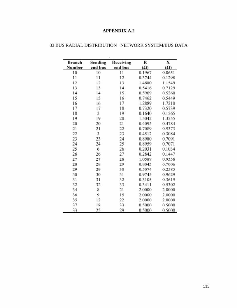
115
APPENDIX A.2
33 BUS RADIAL DISTRIBUTION NETWORK SYSTEM/BUS DATA

116
APPENDIX A.3
33 BUS RADIAL DISTRIBUTION NETWORK LOAD DATA.
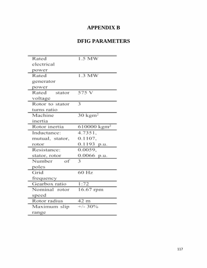
117
APPENDIX B
DFIG PARAMETERS