school of engineering & built environment
TRANSCRIPT

Original Epicyclic and Power Screw notes prepared by G.K. Vijayaraghavan (2006), Original Clutch, Belt and Brake Systems by Dr M. Macdonald, Updated notes prepared by A. Cowell (2017)
School of Engineering & Built Environment
African Leadership College Notes
2017/18
Module: Engineering Design and Analysis 2
Clutch Design and Belt Drives Summary
Dr Andrew Cowell CEng MIMechE FIES Department of Engineering T: 0141 331 3711 E: [email protected]
Page 1 of 6
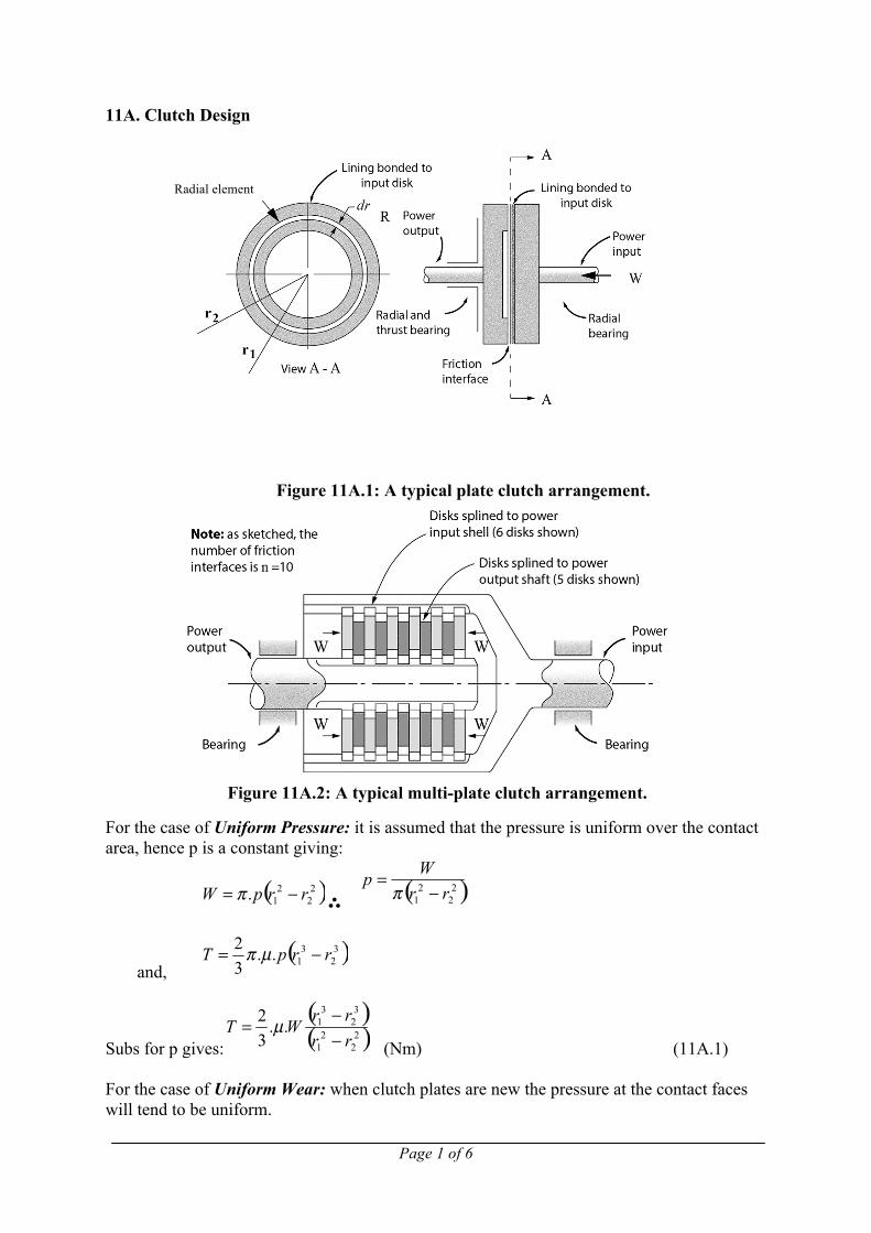
11A. Clutch Design
For the case of Uniform Pressure: it is assumed that the pressure is uniform over the contact area, hence p is a constant giving:
∴
and,
Subs for p gives: (Nm) (11A.1) For the case of Uniform Wear: when clutch plates are new the pressure at the contact faces will tend to be uniform.
Figure 11A.1: A typical plate clutch arrangement.
Figure 11A.2: A typical multi-plate clutch arrangement.
Radial element

Page 2 of 6
T = µWR (Nm) (11A.2) Note: For multi-plate clutches, equations (11A.1) and (11A.2) are multiplied by ‘n’.
Assuming p is constant, i.e. uniform pressure: (Nm) (11A.3) Finally, assuming p.r is constant, i.e. uniform wear:
∴ (Nm) (11A.4) Nomenclature for Clutches Symbol Description Unit A Contact area m2 dr Small portion of contact disc m n Number of contact pairs (plate clutch) - p Intensity of pressure between contact surfaces Nm-2 R Mean radius m r1 Outer radius m r2 Inner radius m T Transmitted torque Nm W Axial thrust force N β Cone angle degrees
Figure 11A.3: A typical cone clutch arrangement.
Page 3 of 6
µ Coefficient of friction -
Page 4 of 6
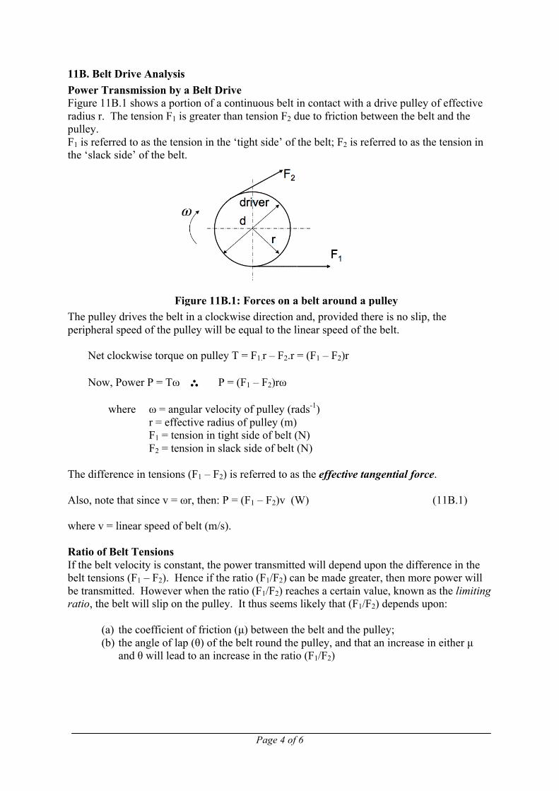
11B. Belt Drive Analysis Power Transmission by a Belt Drive Figure 11B.1 shows a portion of a continuous belt in contact with a drive pulley of effective radius r. The tension F1 is greater than tension F2 due to friction between the belt and the pulley. F1 is referred to as the tension in the ‘tight side’ of the belt; F2 is referred to as the tension in the ‘slack side’ of the belt.
The pulley drives the belt in a clockwise direction and, provided there is no slip, the peripheral speed of the pulley will be equal to the linear speed of the belt. Net clockwise torque on pulley T = F1.r – F2.r = (F1 – F2)r Now, Power P = Tω ∴ P = (F1 – F2)rω where ω = angular velocity of pulley (rads-1) r = effective radius of pulley (m) F1 = tension in tight side of belt (N) F2 = tension in slack side of belt (N) The difference in tensions (F1 – F2) is referred to as the effective tangential force. Also, note that since v = ωr, then: P = (F1 – F2)v (W) (11B.1) where v = linear speed of belt (m/s). Ratio of Belt Tensions If the belt velocity is constant, the power transmitted will depend upon the difference in the belt tensions (F1 – F2). Hence if the ratio (F1/F2) can be made greater, then more power will be transmitted. However when the ratio (F1/F2) reaches a certain value, known as the limiting ratio, the belt will slip on the pulley. It thus seems likely that (F1/F2) depends upon:
(a) the coefficient of friction (µ) between the belt and the pulley; (b) the angle of lap (θ) of the belt round the pulley, and that an increase in either µ
and θ will lead to an increase in the ratio (F1/F2)
Figure 11B.1: Forces on a belt around a pulley

Page 5 of 6
It can be shown that the limiting ratio of tensions (F1/F2) is given by:
(11B.2) where, F1 = tension in tight side of belt (N) F2 = tension in slack side of belt (N) e = constant = 2.718 (base of natural logarithms) µ = coefficient of friction between belt and pulley θ = angle of lap of belt round pulley (rads) Note than where an open belt connects two pulleys of different diameters, the angle of lap on the smaller pulley will be less than that on the larger pulley. From Figure 4.5 it can be seen that θS is less than θL. Figure 11B.2: Angle of lap for drive and driven pulley Calculations, then, would be based on the smallest pulley. Vee-Belt Drives
(a) (b)
Figure 11B.3: Vee belt and pulley interaction The belt tension sets up a radial force R acting towards the centre of the pulley. From Figure 11B.3(b):
θL θS

Page 6 of 6
∴
∴ R = 2RNsinα ∴
Now, for flat belts, the friction force = µR
and for vee-belts, the friction force = 2µRN (two friction surfaces) =
Hence, the belt tension formula for flat belts, is modified for vee-belts and becomes:
where, F1 = tension in tight side of belt (N) F2 = tension in slack side of belt (N) e = constant = 2.718 µ = coefficient of friction between belt and pulley θ = angle of lap of belt round pulley (rads) and, 2α = included angle of pulley groove (°)
Page 7 of 6
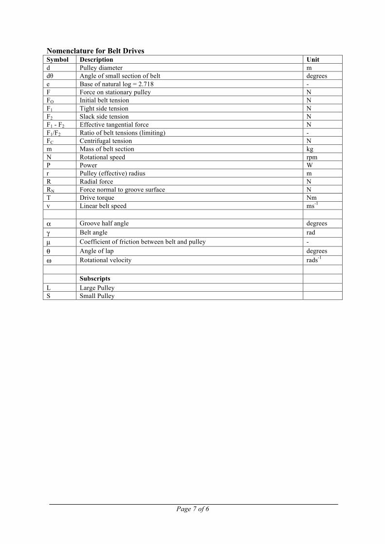
Nomenclature for Belt Drives Symbol Description Unit d Pulley diameter m dθ Angle of small section of belt degrees e Base of natural log = 2.718 - F Force on stationary pulley N FO Initial belt tension N F1 Tight side tension N F2 Slack side tension N F1 - F2 Effective tangential force N F1/F2 Ratio of belt tensions (limiting) - FC Centrifugal tension N m Mass of belt section kg N Rotational speed rpm P Power W r Pulley (effective) radius m R Radial force N RN Force normal to groove surface N T Drive torque Nm v Linear belt speed ms-1 α Groove half angle degrees γ Belt angle rad µ Coefficient of friction between belt and pulley - θ Angle of lap degrees ω Rotational velocity rads-1 Subscripts L Large Pulley S Small Pulley