Working Paper SeriesWP 2008-24

School of Economic Sciences

Washington Biofuel Feedstock Crop Supply Analysis

By

Qiujie Zheng and C. Richard Shumway

December 2008

Washington Biofuel Feedstock Crop Supply Analysis

Qiujie Zheng

C. Richard Shumway

Abstract

Biofuels, as alternative transportation fuels, are now being used globally. Taking advantage of

in-state feedstock supply is an efficient way to stimulate in-state biofuel industries and the local

economy. This paper uses several models to estimate supply equations for major biofuel

feedstock crops in Washington. We estimate expected utility maximization models, expected

profit maximization models, and several pragmatic models. We examine the comparative statics

results of the models, and use the results to draw important implications for Washington policy

makers and for farmers who are considering production of biofuel feedstocks.

Keywords: biofuel feedstock, output uncertainty, price uncertainty, profit maximization, supply

Qiujie Zheng is a graduate research assistant and C. Richard Shumway is a professor in the

School of Economic Sciences, Washington State University.

1

Washington Biofuel Feedstock Crop Supply Analysis

Biofuels, as alternative transportation fuels derived from biomass, are now being used

globally. Biofuels can provide local economic benefits such as additional markets for farm crops

and additional jobs in rural communities. Broader benefits include potential mitigation of

greenhouse gas emissions (under certain scenarios) as well as improvements in energy security

by decreasing dependence on foreign sources of fuels.

Biofuel production and use are in their infancy but are experiencing a period of rapid

growth. New markets are being created to help foster biofuel growth across the United States.

Washington State’s push toward biofuels is evidenced by state and local government mandates,

expansion of state-owned vehicles running on biofuels, increases in the number of biofuel plants,

and increases in the acreage of feedstocks.

Taking advantage of in-state feedstock supply is an efficient way to stimulate in-state

biofuel industries and the local economy. Thus, analyzing the existing feedstock supply and

potential in Washington is important. “Under current technology, Washington’s potential biofuel

crops include corn and sugar beets for sugar-based ethanol; oilseed crops (canola, soybeans,

camelina, mustard, safflower, sunflower and peanuts) for biodiesel; and poplar, grain straw,

switch grass and other fiber sources for cellulosic ethanol.” (Yoder et. al., 2007, p. 7)

Corn ethanol is the major biofuel now used in the United States. In Washington, corn is

primarily grown under irrigation in the Columbia Basin. It is relatively expensive to grow corn in

Washington compared to the Midwest. Although there was a 67% increase in Washington corn

harvested acreage in 2007 compared to 2006, it contributes a trivial part of national production

(about 1/10 of 1 percent). Sugar beets were a common crop produced in Washington until 1978,

but little has been grown since processing facilities were closed due to low sugar prices and high

2

energy costs. The few acres of sugar beets still grown in Washington are near Moses Lake, and

research on the economic potential for sugar beets as a biofuel feedstock is necessary and

underway.

Compared to their experience in growing grains, oilseed crops are comparatively new to

Washington’s farmers. Economic viability and agronomic refinements to plant and harvest

techniques, nutrient inputs, soil management, and weed and pest control are just beginning

(Washington State Biofuels Advisory Committee Report. August 2007). Canola has the highest

oil yield of the various oilseed crops and has been grown in limited quantities for several decades

in Washington. Mustard and safflower have lower oil yields than canola. Soybeans can be grown

in the warmer southern portion of the Columbia Basin but only under irrigation. Camelina,

sunflower and peanuts are under cropping trials in the State.

The final type of biofuel feedstock is cellulosic biomass, inedible plants grown on less than

optimal farmland. Use of cellulosic feedstock will mitigate the food versus fuel problem but will

take time for producers to gain experience to grow and for researchers and processors to innovate

with improved technologies to convert cellulose to fuel. We do not consider cellulosic feedstock

supplies in this paper.

With more farmers considering production of biofuel feedstocks, an examination of their

supply response is critical for purposes of predicting future crop prices as well as food and fuel

supplies. The high demand for biofuel production that may or may not persist could drive

feedstock prices to be high and variable which will play an important role in farmers’ planting

decisions. Thus, the analysis of biofuel feedstock supplies must take crop price and output

uncertainty into account.

Much research has focused on crop supplies. Some studies have incorporated output price

3

or quantity risk into the economic models of supply. This paper develops several models under

utility maximization considering output and/or price uncertainty or under profit maximization

without risk to examine the supply of major biofuel feedstocks in Washington. Its purpose is to

predict supply response and guide Washington farmers in making optimal production decisions

as the biofuel industry develops in the State. Our objectives are to (a) estimate supply equations

for major biofuel feedstock crops, (b) examine the comparative statics results of the models, and

(c) use the results to draw important decision-making implications for Washington farmers who

are considering production of biofuel feedstock crops.

Relevant Literature

The research literature on crop supplies under risk is extensive. We will illustrate the extent

of this literature by citing just a few and will give relatively greater emphasis to literature that

has addressed both profit and risk motives.

Just (1974) generalized the adaptive expectations geometric lag model by including

quadratic lag terms indicative of risk and applied the model to the analysis of California

field-crop supply response. Pope (1982) addressed conceptual and estimation issues to develop

procedures for incorporating risk into a wide range of production economic models and

procedures.

Chavas and Holt (1990) developed an acreage supply response model under expected utility

maximization considering price and yield uncertainty using subjective probability distributions

and investigated its empirical implications for U.S. corn and soybean acreages. Pope and Just

(1991) proposed an econometric test for distinguishing the class of preferences and implemented

it for potato supply response in Idaho. Meyers and Robison (1991) extended the theory of the

firm facing a random output price to include industry equilibrium conditions and developed an

4

aggregate model under risk which displays the linkages between risk, return and land prices.

Coyle (1992) developed tractable dual models of production under risk aversion and price

uncertainty within the context of a mean-variance model of utility maximization. Saha,

Shumway and Talpaz (1994) used an expo-power utility function to jointly estimate risk

preference structure, degree of risk aversion and production technology and implemented it for a

sample of Kansas wheat farmers. Chavas and Holt (1996) developed a maximum likelihood

procedure to jointly estimate risk preferences and technology under very general conditions and

used it to examine U.S. corn-soybean acreage decisions.

Saha and Shumway (1998) derived the complete set of refutable propositions for the

competitive firm model under a general wealth structure that encompasses output price and

quantity risk as special cases and empirically tested some of the propositions using firm-level

data. Adrangi and Raffiee (1999) developed a general model of the competitive firm’s behavior

under output and factor price uncertainty to evaluate the role of market interdependencies in

analyzing long-run equilibrium conditions and the comparative statics of increased uncertainty in

output and input prices. Kumbhakar (2002) dealt with specification and joint estimation of risk

preferences, production risk, and technical inefficiency. Alghalith (2007) modified and expanded

the duality theory and implemented a tractable empirical procedure for estimating supply

response and testing hypotheses under both price and output uncertainty.

In this study, we will consider output price and quantity risk motivations in our model of

expected utility maximization. We will also consider both risks associated with the feedstock

commodity as well as the influence of risks from rotational crops to estimate the optimal supply

response. Alternative models will maintain the hypothesis that producers are risk-neutral,

profit-maximizing firms. They will be developed and estimated subject to various restrictions

5

implied by profit maximization.

Data

The primary biofuel feedstock crops currently being grown in Washington or being given

serious consideration by farmers are corn, sugar beets and canola. State-level annual data for

these crops and their primary rotational crops are used in the analysis. We consider three

rotational pairs – corn and potatoes, sugar beets and alfalfa hay, canola and wheat. The

production data for corn, potatoes and alfalfa hay and the market price data for potatoes and

alfalfa hay for Washington from 1960 to 2006 are from the USDA National Agricultural

Statistics Service (NASS). The production data for sugar beets, market price data and

government program payments for corn and sugar beets, and aggregate input price index data for

Washington from 1960 to 2004 were compiled by Eldon Ball (Ball, Hallahan, and Nehring 2004).

We extended these data to 2005 and 2006 using USDA NASS price and quantity data and Eldon

Ball’s tabulation of government program payments.

Since time series data for U.S. and state-level canola production do not exist for this length

of time, we use annual data for four states from 1992 to 2004. State-level production, market

price, government program payments and aggregate input price index data for canola and wheat

for Washington, Idaho, Minnesota and North Dakota are from Eldon Ball.

Public research data for each state for the period 1961-2004 are from Wallace Huffman.

These data represent the estimated investment stock values of public research expenditures and

were calculated based on a trapezoidal function of past expenditures (Huffman and Evenson

1989). Because the stock of public research investment was nearly constant during the final five

years, the stock for 2005 and 2006 was presumed to be the same as for 2004.

6

Method of Analysis

We estimate supply equations for three pairs of crops commonly grown in rotation in

Washington. They include corn and potatoes, sugar beets and alfalfa hay, canola and wheat. We

have enough observations for corn, potatoes, sugar beets and alfalfa hay to introduce output price

and quantity risk along with profit into an expected utility function. Farmers are expected to be

risk averse and maximize the expected utility of profit and uncertainty. We use Model 1 to

estimate supply functions accounting for both output price and quantity risks, Model 2 to

estimate supply functions under both output price risk and risk-neutral profit maximization,

Model 3 to estimate supply functions under risk-neutral profit maximization using panel data,

and Model 4 (a set of pragmatic models) to estimate supply functions while maintaining the most

important expectation under profit maximization (i.e., that own-price supplies are upward

sloping and statistically significant).

Because of limited data for canola, we use panel data and estimate supply equations for

canola and wheat based only on risk-neutral profit maximization (Model 3) using a multi-state

panel model. We use this model to focus on Washington supply response of canola.

Model 1 – Expected Utility Maximization under Output Price and Quantity Risk

Consider a farmer with two rotational crops. When she is making her planting decisions, she

faces uncertain output prices given by i i i ip p σ ε= + , where 1,2i = denotes two rotational

crops, iε is random with [ ] 0iE ε = and [ ] 1iVar ε = ; thus, [ ]i iE p p= and 2[ ]i iVar p σ= . The

output level realized at harvest time is also uncertain due mainly to variability in weather, soil,

pests, and disease. We denote output as i i i i i i iq q yθη θη= + = + , where iη is random with

[ ] 0iE η = and [ ] 1iVar η = , so that [ ]i i iE q q y= = and 2[ ]i iVar q θ= . Input prices are known

with certainty at planting time, and costs are represented by a cost function, ( , )i ic y w , where iy

7

is expected output for one crop and w is the state-level aggregate input price. The farmer can

estimate individual crop costs at planting from expected crop output level and aggregate input

price.

The profit function for this farm manager is:

(1) 1 1 2 2 1 1 2 2( , ) ( , ).p q p q c y w c y wπ = + − −

We assume this farm manager is risk averse and maximizes the expected utility of profit:

(2) 1 2

1 1 2 2 1 1 2 2,[ ( )] [ ( ( , ) ( , ))].

y yMax E U E U p q p q c y w c y wπ = + − −

Assuming that standard regularity conditions apply to the technology, there exist optimal

expected output levels *1y and *

2y that maximize profit

* * * * *1 1 1 1 2 2 2 2 1 1 2 2( ) ( ) ( , ) ( , )p y p y c y w c y wπ θη θ η= + + + − − . Thus we can get the indirect expected

utility function with profit-maximizing expected output levels:

(3) 1 2 1 2 1 2* * * *

1 1 1 1 2 2 2 2 1 1 2 2

( , , , , , , )[ ( ( ) ( ) ( , ) ( , ))].

V p p wE U p y p y c y w c y w

σ σ θ θ

θη θ η= + + + − −

Applying the envelope theorem to (3), we obtain the first derivatives of indirect expected

utility to expected prices of the crops. For the first crop:

(4) 1

* * *1 1 1

1

[ ( )] [ ( ) ].pV V y E U E Up

π θ π η∂ ′ ′= = +∂

If there is only price risk, we can derive a supply function directly from (4) since 1η will

be zero in that case. However, with 1η also a random term representing output uncertainty, we

use the second-order Taylor’s series expansion to deal with the second term in (4).

Consider an approximation of *( )U π′ around the arbitrary point π̂ :

(5) * *ˆ ˆ ˆ( ) ( ) ( )( ).U U Uπ π π π π′ ′ ′′≈ + −

8

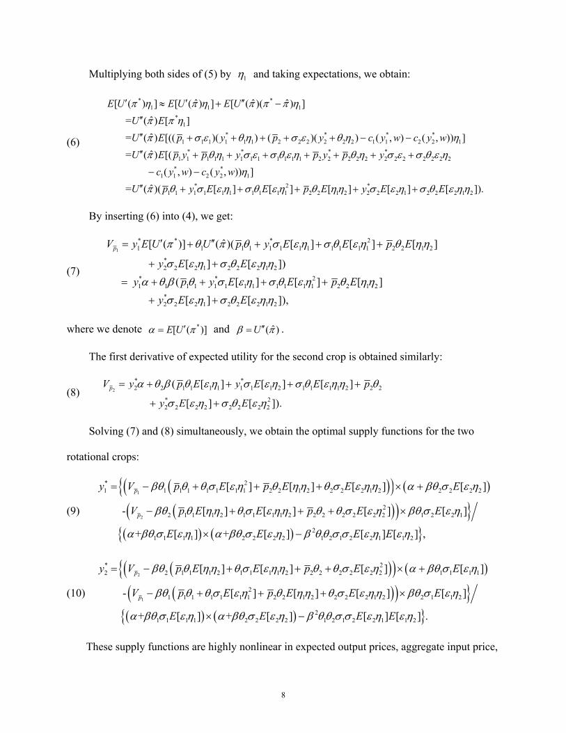
Multiplying both sides of (5) by 1η and taking expectations, we obtain:

(6)

* *1 1 1

*1

* * * *1 1 1 1 1 1 2 2 2 2 2 2 1 1 2 2 1

* * *1 1 1 1 1 1 1 1 1 1 1 1 2 2

ˆ ˆ ˆ[ ( ) ] [ ( ) ] [ ( )( ) ]ˆ = ( ) [ ]ˆ = ( ) [(( )( ) ( )( ) ( , ) ( , )) ]ˆ = ( ) [(

E U E U E U

U EU E p y p y c y w c y wU E p y p y p y

π η π η π π π η

π π η

π σ ε θη σ ε θ η η

π θη σ ε σ θ ε η

′ ′ ′′≈ + −

′′

′′ + + + + + − −

′′ + + + + + *2 2 2 2 2 2 2 2 2 2

* *1 1 2 2 1

* 2 *1 1 1 1 1 1 1 1 1 1 2 2 1 2 2 2 2 1 2 2 2 1 2

( , ) ( , )) ]ˆ = ( )( [ ] [ ] [ ] [ ] [ ]).

p yc y w c y w

U p y E E p E y E E

θ η σ ε σ θ ε η

η

π θ σ ε η σ θ ε η θ ηη σ ε η σ θ ε ηη

+ +

− −

′′ + + + + +

By inserting (6) into (4), we get:

(7)

1

* * * 21 1 1 1 1 1 1 1 1 1 1 1 2 2 1 2

*2 2 2 1 2 2 2 1 2

* * 21 1 1 1 1 1 1 1 1 1 1 1 2 2 1 2

*2 2 2 1 2 2

ˆ[ ( )] ( )( [ ] [ ] [ ]

[ ] [ ]) ( [ ] [ ] [ ] [ ]

pV y E U U p y E E p E

y E Ey p y E E p E

y E

π θ π θ σ ε η σ θ ε η θ ηη

σ ε η σ θ ε ηη

α θ β θ σ ε η σ θ ε η θ ηη

σ ε η σ θ

′ ′′= + + + +

+ +

= + + + +

+ + 2 1 2[ ]),E ε ηη

where we denote *[ ( )]E Uα π′= and ˆ( )Uβ π′′= .

The first derivative of expected utility for the second crop is obtained similarly:

(8) 2

* *2 2 1 1 1 1 1 1 1 2 1 1 1 1 2 2 2

* 22 2 2 2 2 2 2 2

( [ ] [ ] [ ]

[ ] [ ]).pV y p E y E E p

y E E

α θ β θ ε η σ ε η σ θ ε ηη θ

σ ε η σ θ ε η

= + + + +

+ +

Solving (7) and (8) simultaneously, we obtain the optimal supply functions for the two

rotational crops:

(9)

( )( ) ( ){( )( ) }

( ) ( )

1

2

* 21 1 1 1 1 1 1 1 2 2 1 2 2 2 2 1 2 2 2 2 2

22 1 1 1 2 1 1 1 1 2 2 2 2 2 2 2 1 2 2 1

21 1 1 1 2 2 2 2 1 2 1 2 2 1 1

[ ] [ ] [ ] [ ]

- [ ] [ ] [ ] [ ]

+ [ ] + [ ] [ ] [

p

p

y V p E p E E E

V p E E p E E

E E E E

βθ θ θ σ ε η θ ηη θ σ ε ηη α βθ σ ε η

βθ θ ηη θ σ ε ηη θ θ σ ε η βθ σ ε η

α βθ σ ε η α βθ σ ε η β θ θ σ σ ε η ε η

= − + + + × +

− + + + ×

× −{ }2 ] ,

(10)

( )( ) ( ){( )( ) }

( ) ( )

2

1

* 22 2 1 1 1 2 1 1 1 1 2 2 2 2 2 2 2 1 1 1 1

21 1 1 1 1 1 1 2 2 1 2 2 2 2 1 2 2 1 1 2

21 1 1 1 2 2 2 2 1 2 1 2 2 1 1

[ ] [ ] [ ] [ ]

- [ ] [ ] [ ] [ ]

+ [ ] + [ ] [ ] [

p

p

y V p E E p E E

V p E p E E E

E E E E

βθ θ ηη θ σ ε ηη θ θ σ ε η α βθ σ ε η

βθ θ θ σ ε η θ ηη θ σ ε ηη βθ σ ε η

α βθ σ ε η α βθ σ ε η β θ θ σ σ ε η ε

= − + + + × +

− + + + ×

× −{ }2 ] .η

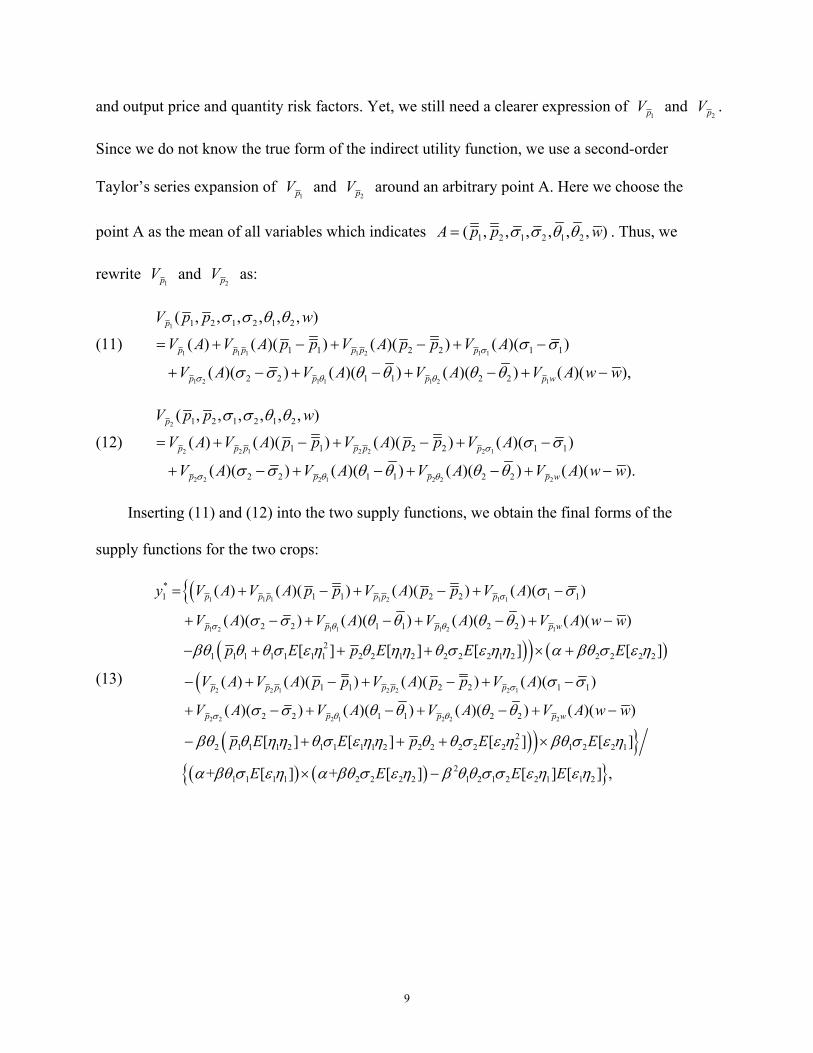
These supply functions are highly nonlinear in expected output prices, aggregate input price,

9

and output price and quantity risk factors. Yet, we still need a clearer expression of 1pV and

2pV .

Since we do not know the true form of the indirect utility function, we use a second-order

Taylor’s series expansion of 1pV and

2pV around an arbitrary point A. Here we choose the

point A as the mean of all variables which indicates 1 2 1 2 1 2( , , , , , , )A p p wσ σ θ θ= . Thus, we

rewrite 1pV and

2pV as:

(11) 1

1 1 1 1 2 1 1

1 2 1 1 1 2 1

1 2 1 2 1 2

1 1 2 2 1 1

2 2 1 1 2 2

( , , , , , , )

( ) ( )( ) ( )( ) ( )( )

( )( ) ( )( ) ( )( ) ( )( ),

p

p p p p p p

p p p p w

V p p w

V A V A p p V A p p V A

V A V A V A V A w wσ

σ θ θ

σ σ θ θ

σ σ

σ σ θ θ θ θ

= + − + − + −

+ − + − + − + −

(12) 2

2 2 1 2 2 2 1

2 2 2 1 2 2 2

1 2 1 2 1 2

1 1 2 2 1 1

2 2 1 1 2 2

( , , , , , , )

( ) ( )( ) ( )( ) ( )( )

( )( ) ( )( ) ( )( ) ( )( ).

p

p p p p p p

p p p p w

V p p w

V A V A p p V A p p V A

V A V A V A V A w wσ

σ θ θ

σ σ θ θ

σ σ

σ σ θ θ θ θ

= + − + − + −

+ − + − + − + −

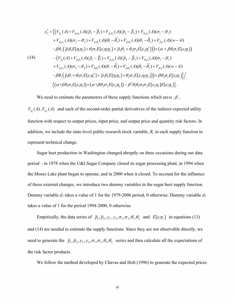
Inserting (11) and (12) into the two supply functions, we obtain the final forms of the

supply functions for the two crops:

(13)

({

( )) ( )

1 1 1 1 2 1 1

1 2 1 1 1 2 1

*1 1 1 2 2 1 1

2 2 1 1 2 2

21 1 1 1 1 1 1 2 2 1 2 2 2 2 1 2 2 2 2 2

( ) ( )( ) ( )( ) ( )( )

( )( ) ( )( ) ( )( ) ( )( )

[ ] [ ] [ ] [ ]

p p p p p p

p p p p w

y V A V A p p V A p p V A

V A V A V A V A w w

p E p E E E

σ

σ θ θ

σ σ

σ σ θ θ θ θ

βθ θ θ σ ε η θ ηη θ σ ε ηη α βθ σ ε η

= + − + − + −

+ − + − + − + −

− + + + × +

(

( )) }

2 2 1 2 2 2 1

2 2 2 1 2 2 2

1 1 2 2 1 1

2 2 1 1 2 2

22 1 1 1 2 1 1 1 1 2 2 2 2 2 2 2 1 2 2 1

( ) ( )( ) ( )( ) ( )( )

( )( ) ( )( ) ( )( ) ( )( )

[ ] [ ] [ ] [ ]

p p p p p p

p p p p w

V A V A p p V A p p V A

V A V A V A V A w w

p E E p E E

σ

σ θ θ

σ σ

σ σ θ θ θ θ

βθ θ ηη θ σ ε ηη θ θ σ ε η βθ σ ε η

− + − + − + −

+ − + − + − + −

− + + + ×

( ) ( ){ }21 1 1 1 2 2 2 2 1 2 1 2 2 1 1 2 + [ ] + [ ] [ ] [ ] ,E E E Eα βθ σ ε η α βθ σ ε η β θ θ σ σ ε η ε η× −

10

(14)

({

( )) ( )

2 2 1 2 2 2 1

2 2 2 1 2 2 2

*2 1 1 2 2 1 1

2 2 1 1 2 2

22 1 1 1 2 1 1 1 1 2 2 2 2 2 2 2 1 1 1 1

( ) ( )( ) ( )( ) ( )( )

( )( ) ( )( ) ( )( ) ( )( )

[ ] [ ] [ ] [ ]

p p p p p p

p p p p w

y V A V A p p V A p p V A

V A V A V A V A w w

p E E p E E

σ

σ θ θ

σ σ

σ σ θ θ θ θ

βθ θ ηη θ σ ε ηη θ θ σ ε η α βθ σ ε η

= + − + − + −

+ − + − + − + −

− + + + × +

(

( )) }

1 1 1 1 2 1 1

1 2 1 1 1 2 1

1 1 2 2 1 1

2 2 1 1 2 2

21 1 1 1 1 1 1 2 2 1 2 2 2 2 1 2 2 1 1 2

( ) ( )( ) ( )( ) ( )( )

( )( ) ( )( ) ( )( ) ( )( )

[ ] [ ] [ ] [ ]

p p p p p p

p p p p w

V A V A p p V A p p V A

V A V A V A V A w w

p E p E E E

σ

σ θ θ

σ σ

σ σ θ θ θ θ

βθ θ θ σ ε η θ ηη θ σ ε ηη βθ σ ε η

α

− + − + − + −

+ − + − + − + −

− + + + ×

( ) ( ){ }21 1 1 1 2 2 2 2 1 2 1 2 2 1 1 2+ [ ] + [ ] [ ] [ ] .E E E Eβθ σ ε η α βθ σ ε η β θ θ σ σ ε η ε η× −

We need to estimate the parameters of these supply functions which areα ,β ,

1( )pV A ,

2( )pV A and each of the second-order partial derivatives of the indirect expected utility

function with respect to output prices, input price, and output price and quantity risk factors. In

addition, we include the state-level public research stock variable, R, in each supply function to

represent technical change.

Sugar beet production in Washington changed abruptly on three occasions during our data

period – in 1978 when the U&I Sugar Company closed its sugar processing plant, in 1994 when

the Moses Lake plant began to operate, and in 2000 when it closed. To account for the influence

of these external changes, we introduce two dummy variables in the sugar beet supply function.

Dummy variable d1 takes a value of 1 for the 1979-2006 period, 0 otherwise. Dummy variable d2

takes a value of 1 for the period 1994-2000, 0 otherwise.

Empirically, the data series of 1 2 1 2 1 2 1 2, , , , , , ,p p y y σ σ θ θ and [ ]i jE εη in equations (13)

and (14) are needed to estimate the supply functions. Since they are not observable directly, we

need to generate the 1 2 1 2 1 2 1 2, , , , , , ,p p y y σ σ θ θ series and then calculate all the expectations of

the risk factor products.

We follow the method developed by Chavas and Holt (1996) to generate the expected prices

11

series, 1p and 2p , for the Model 1 equations, where the price at time t is regressed on its

lagged price.

(15) 1 1,2,it i i it itp p u iγ λ −= + + =

where itp is the market price plus government programs payment for crop i at time t , 1itp −

is crop i ’s previous year’s price, iγ and iλ are drift and slope parameters for crop i , itu is

error term with [ ] 0itE u = . Hence, the expected prices are:

(16) 1[ ] 1, 2.it it i i itE p p p iγ λ −= = + =

We use a similar method (Lapan and Moschini 1994) to generate the expected output series,

1y and 2y , where output at time t is also dependent on their lagged values:

(17) 1 1,2,it i i it itq q v iφ ϕ −= + + =

where itq is the output level for crop i at time t , 1itq − is crop i ’s previous year’s output

level, iφ and iϕ are drift and slope parameters for crop i , itv is error term with [ ] 0itE v = .

Thus, the expected outputs are:

(18) 1[ ] 1,2.it it i i itE q y q iφ ϕ −= = + =

We follow Chavas and Holt’s (1996) method to generate risk factors 1 2 1 2, , ,σ σ θ θ .

(19) 3

2 2

1

( ) 1,2,it j it j it j it jj

p E p iσ ω − − −=

= − =∑

(20) 3

2 2

1

( ) 1,2,it j it j it j it jj

q E q iθ ω − − −=

= − =∑

where jω are 0.5, 0.33, 0.17 when 1, 2,3j = . The variances of price and output are measured

as a declining weighted sum of the squared difference of previous real values from expected

values.

12

Then from the price equations, i i i ip p σ ε= + , 1, 2i = , and output equations,

i i i i i i iq q yθη θη= + = + , 1, 2i = , together with (19) and (20), we can calculate all the

expectations of the products of risk factors in (13) and (14).

With these generated values of the independent and dependent variables and the formulas

for the nonlinear supply response functions, we use nonlinear seemingly unrelated least squares

to estimate the supply functions of the two rotational crops. We use this estimated model to not

only calculate estimated supply elasticities but also to test several hypotheses about producer

motivations. For example, if the producer is risk neutral, then ˆ''( ) 0U π β= = and expected

utility does not depend on output price or quantity risk, which means 0i

Vσ = and 0i

Vθ = . This

implies that all the partial derivatives of i

Vσ and i

Vθ are also zero. Thus, we test risk neutrality

by:

(21) 1 1 1 2 2 1 2 2 1 1 1 2 2 1 2 2

0.p p p p p p p pV V V V V V V Vσ σ σ σ θ θ θ θβ = = = = = = = = =

We test for the absence of output price risk by:

(22) 1 1 1 2 2 1 2 2

0,p p p pV V V Vσ σ σ σ= = = =

and the absence of output quantity risk by:

(23) 1 1 1 2 2 1 2 2

0.p p p pV V V Vθ θ θ θ= = = =

Model 2 – Expected Utility Maximization under Output Price Risk

In this model, we ignore output quantity uncertainty while assuming farmers are risk averse

and seek to maximize their expected utility considering output price risk only. We also impose

some structure following Coyle (1992) by specifying a mean-variance utility function with

stochastic output prices that is linear in expected profits, E[π], and profit variance, V[π]:

(24) [ ] [ ]2

U E Vαπ π= −

13

where α is a measure of risk aversion.

As in Model 1, the producer plants two rotational crops using an aggregate input. The

farmer’s profit function is:

(25) 1 1 2 2p q p q wxπ = + −

where p1, p2 are crop prices (market prices adjusted for government programs payments), q1, q2

are crop output levels, w is aggregate input price, and x is aggregate input level. Hence,

(26) 1 2 1 1 2 2[ ( , , )]E q q x p q p q wxπ = + −

(27) 2 21 2 1 1 2 2 1 2 1 2[ ( , , )] ( ) ( ) 2 ( , )V q q x q var p q var p q q cov p pπ = + +

where 1 2,p p are expected crop prices (including government program payments) at planting

time, var(p1), var(p2), cov(p1,p2) are variances and covariance of the crop prices.

The farmer is risk averse and maximizes her expected utility:

(28) { }

1 2

*1 2 1 2 1 2

2 21 2 1 1 2 2 1 1 2 2 1 2 1 2, ,

( , , , var( ), var( ),cov( , ))

max ( , , ) ( ) ( ) 2 ( , )2q q x

U p p w p p p p

U q q x p q p q wx q var p q var p q q cov p pα ⎡ ⎤= = + − − + +⎣ ⎦

The following propositions apply to this dual specification of the price taking, risk averse,

expected-utility maximizing producer:

(a) *U is increasing in p , decreasing in w , decreasing in Vp , where Vp is the

covariance matrix of crop prices.

(b) *U is linear homogeneous in ( , , )p w Vp .

(c) *U is convex in prices p and w .

(d) *( )U ⋅ is differentiable as follows:

(29) *

*( , , ) , 1, 2.jj

U p w Vp q jp

∂= =

∂

14

(30) *( , , )U p w Vp x

w∂

= −∂

(31) *

*2( , , ) , 1, 2.2 j

jj

U p w Vp q jVp

α∂= − =

∂

(32) *

* *( , , ) , ; , 1, 2.i jij

U p w Vp q q i j i jVp

α∂= − ≠ =

∂

By specifying functional forms for the derivatives of this dual model with respect to prices p and w ,

we can get specific functional forms for the derivatives of the dual with respect to the elements of Vp ,

and can trace backwards to the dual utility function by Euler’s theorem.

First we define general forms for the partial derivatives.

(33)

1 2 1 2 1 2

1 2 1 2 1 2

var( ) var( ) cov( , ), , , , , 1, 2.

var( ) var( ) cov( , ), , , ,

j jp p p p p pq q jw w w w w

p p p p p px xw w w w w

⎛ ⎞= =⎜ ⎟⎝ ⎠

⎛ ⎞= ⎜ ⎟⎝ ⎠

Since we do not have input quantity data for our specific crops, we are unable to estimate

the input demand equation. Using seemingly unrelated regression method (SUR), we estimate

the following system of supply functions, which are generalizations of those derived from a

normalized quadratic profit function:

(34)

1 1 2 1 1 2 1 21 1 11 12 13 11 12 13 1

1 1 2 1 1 2 1 22 2 21 22 23 21 22 23 2

var( ) var( ) cov( , )

var( ) var( ) cov( , )

t t t t t tt t

t t t t t

t t t t t tt t

t t t t t

p p p p p pq a a a a R b b b uw w w w wp p p p p pq a a a a R b b b uw w w w w

− −

− −

= + + + + + + +

= + + + + + + +

where R is the state level research stock variable. Assuming a Markov process, farmers take each

crop’s lagged price (adjusted for government payments) as the expected price for Model 2-4

equations. Consistent with proposition (b) of the utility function, this specification maintains the

property that each supply function is homogeneous of degree zero in prices, variance, and

15

covariance by dividing each of these variables by the input price index. Consistent with

proposition (c), we maintain the property that the system of supply functions is convex in prices

by reparameterizing the parameter matrix on the price variables using the Cholesky

decomposition method. Consistent with proposition (d), we impose symmetry restrictions on the

cross-price equations.

We derive variances and covariance of the crop prices following Chavas and Holt (1996)

and introduce the same dummy variables in the sugar beets supply equation as in Model 1. We

estimate and analyze the estimation results both under expected utility maximization (i.e., when

we include the price variance and covariance items in equation (33)) and under risk-neutral profit

maximization (i.e., when bij=0, i=1,2; j=1,2,3). We test for risk neutrality by testing the

hypothesis that the coefficients on the variance and covariance terms are jointly zero.

Model 3 – Profit Maximization

We use panel data and estimate supply equations for canola and wheat based on profit

maximization in a multi-state panel model. Because of the extremely limited time series for

canola price and production data in each state, we do not introduce price risk into the supply

functions but maintain the assumption of linear supply functions. Under price-taking,

profit-maximizing behavior, the supply equations are nondecreasing in output prices,

nonincreasing in aggregate input price, homogeneous of degree zero in prices, and convex in

prices. If the profit function is twice continuously differentiable, the cross-price parameters are

symmetric between the linear supply functions. Thus, we estimate the following supply functions

as a fixed-effects panel data model allowing for differences between states in all parameters:

16

(37)

1 1 2 11 1 11 12 13 1

1 1 2 12 2 21 22 23 2

mt mtmt m m m m mt t

mt mt

mt mtmt m m m m mt t

mt mt

p pq a a a a R vw wp pq a a a a R vw w

− −

− −

= + + + +

= + + + +

where m=WA, ID, MN, ND denotes Washington, Idaho, Minnesota, and North Dakota,

respectively.

We also estimate this system of supply equations as a system of seemingly unrelated

regressions. While we obtain results for all four states, we focus on the implications for

Washington.

Model 4 – Pragmatic Alternatives

In addition to models that fully satisfy the expected utility or the profit maximization

hypotheses, we also search for specifications of Washington corn and sugar beet supplies that

meet the most important expectation under profit maximization, i.e., a positively-sloped

own-price parameter, that is statistically significant. We focus attention on models that permit

the short-run and long-run price elasticities to be distinguished; assuming Koyck distributed lags,

the lagged dependent variable is included in the specification as a regressor. We consider simple

linear and loglinear specifications based on profit maximization or expected utility maximization.

Following a Markov process, lagged output prices (market plus government payments) are the

expected output prices. So the basic specification is as follows:

(38) *1 1it i ii it ij jt iy it

j

q a a p a p a q− −= + + +∑

where p* is a subset of the vector of other expected output prices, the input price index, and

research stock or year. In some cases the expected output prices are divided by the input price

index, thus maintaining homogeneity of degree zero as also implied by expected profit

maximization.

17

We estimate Models 1-4 using state-level data. Depending on the model, we maintain the

hypothesis that each state acts as though it were an optimizing (either expected utility, profit, or

quasi-profit maximizing) producer. While the assumption that a state acts as though it were an

optimizing producer is an important abstraction from reality, Lim and Shumway’s (1992)

nonparametric test results failed to reject the most binding version of this hypothesis for the State

of Washington.

Results

In this section, we report and discuss implications of the estimated Washington parameters

for corn and potato supplies and for sugar beet and alfalfa hay supplies based on Models 1, 2 and

4. We report similar findings for canola and wheat for each of four states based on Model 3.

Results from Model 1

Estimated parameters for the Washington corn and potato supply equations, estimated

elasticities, and hypothesis tests from Model 1 are reported in Table 1. Twelve of the 19

parameter estimates are statistically significant at the 10% level (ten at the 5% level). The corn

own-price elasticity is also significant, but it is negative which implies a downward sloping

output supply contrary to strong theoretical expectations. The potato own-price elasticity is also

negative although statistically insignificant. Hypotheses of risk neutrality and absence of either

output price or output quantity risk are all rejected.

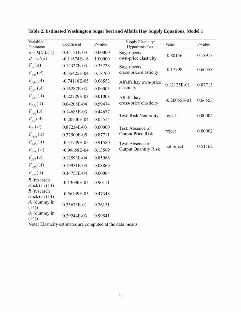
Estimated parameters, elasticities, and hypothesis tests for the Washington sugar beet and

alfalfa hay supply equations from Model 1 are reported in Table 2. Although two more

parameters are estimated in this system of equations, only seven are statistically significant at the

10% level (five at the 5% level). Sugar beet own-price elasticity is negative but insignificantly

different from zero. The alfalfa hay own-price elasticity is positive but also insignificant. Of the

18

three hypotheses tested, only the absence of output quantity risk is not rejected.

Given the small number of statistically significant parameters in the sugar beet – alfalfa hay

equations and the failure of Model 1 to provide positively-sloped estimates of the own-price

elasticity of either biofuel feedstock, we must conclude that this model does not provide a

statistically adequate or economically meaningful fit of the data. Consequently, we turn to other

models of supply for these commodities.

Results from Model 2

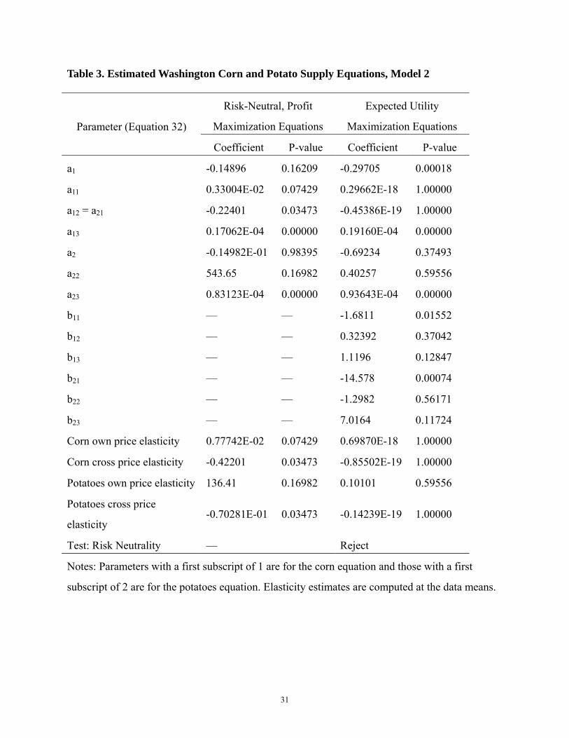
Model 2 parameter estimates for corn and potato supply functions are reported in Table 3.

Two sets of estimates are provided. The first presumes that producers are risk-neutral in

maximizing expected utility (i.e., they maximize expected profit) while the second presumes

they also account for price risk in maximizing expected utility.

Under risk neutrality, four of the seven parameter estimates are statistically significant at the

10% level (three at the 5% level). Except for the intercept, all parameters in the corn supply

equation are statistically significant. The own-price and cross-price elasticities are also

significant. The corn own-price elasticity is small while the potato own-price elasticity is very

large but statistically insignificant. The cross-price elasticities are negative, implying the two

crops are substitutes. We also observe that corn supply is more dependent on potato price than

corn price. Although the magnitude of the own-price elasticity estimate is small for corn and

large for potatoes, when considered along with the cross-price elasticities, they do reflect one

important point. Corn is a very low-value crop relative to potatoes and is often grown as a

rotation crop with potatoes. Thus, it is expected potato price that drives the production of

potatoes. And, since they are grown in rotation, it also drives the production of corn.

We next examine whether price risk is statistically significant and whether it moderates the

19

supply elasticity estimates. When supply response is couched within the framework of

maximizing expected utility under output price risk, five of 13 parameters estimates are

statistically significant at the 10% level (and at the 5% level). However, only one intercept

parameter and the parameters on the research stock and corn variance are significant.

Consequently, although positive, neither own-price elasticity is statistically significant. The

hypothesis of risk neutrality is rejected, which implies that the expected utility maximization

framework is preferred to the assumption of risk-neutral, profit-maximizing behavior. Thus, our

assessment of the historical data via each of the three estimated sets of Model 1 and Model 2

supply equations suggests that Washington corn is unlikely to become a major source of biofuel

feedstock.

Table 4 provides the estimation results for the sugar beet and alfalfa hay supply equations

both under risk neutrality and when considering price risk. Under risk neutrality, five of nine

parameter estimates are significant at the 10% level (five also at the 5% level). Except for the

alfalfa hay price and the second dummy variable, all parameter estimates in the sugar beet

equation are significant. The sugar beet own-price elasticity is significant and approximately

unitary while the alfalfa hay own-price elasticity is small and insignificant.

When output price risk is considered, seven of 15 parameter estimates are statistically

significant. They include the parameters on sugar beet price and variance in the sugar beet

equation. The sugar beet own-price elasticity is again significant and a little larger than when

estimated under the assumption of price neutrality. The price covariance terms were insignificant

in both supply functions, so they were dropped and the supply equations considering price

variances were re-estimated. The drop of covariance terms doesn’t change the results much. The

same parameters are statistically significant, and the sugar beet own-price elasticity is significant

20

and unitary. The hypothesis of risk neutrality is rejected in favor of expected utility

maximization with output price risk.

The relatively large and consistent magnitudes of the Model 2 own-price elasticity estimates

for sugar beets suggest that this crop has potential to become a major biofuel feedstock in

Washington. Its supply can be encouraged by an increase in the market price and/or the

government subsidy.

Results from Model 3

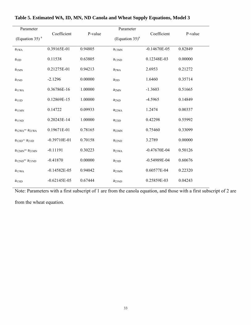
The parameter estimates for Washington, Idaho, Minnesota, and North Dakota wheat and

canola supply equations are reported in Table 5. Only seven of the 28 parameter estimates are

significant at the 10% level (six at the 5% level). They include five parameters for North Dakota

supplies, the canola own-price parameter for Minnesota, and the wheat own-price parameter for

Washington.

Elasticity estimates at the data means are reported in Table 6. The only significant elasticity

in Washington is the wheat own-price elasticity. The canola own-price elasticity is economically

trivial as well as statistically insignificant. The cross-price elasticity is positive which implies

wheat and canola are complements, but it is statistically insignificant. Qualitative results for

Idaho are similar to Washington as is the estimated canola own-price elasticity magnitude. Only

in Minnesota is the canola own-price elasticity significant. Although North Dakota produced

more than 90% of the U.S. canola crop in 2004, its own-price elasticity is trivial and insignificant,

but its cross-price elasticity and wheat own-price and cross-price elasticity are significant. In

North Dakota, canola and wheat are substitutes, and canola production is much more sensitive to

wheat price than to its own price.

Washington contributed 0.35% of the U.S. canola production and 6.65% of U.S. wheat

21

production in 2004. The State’s canola supply is trivial, and our analysis suggests that it

currently is largely unresponsive to its expected price. Other recent empirical evidence supports

this finding by noting that high production risks associated with producing this crop in Eastern

Washington make it uncompetitive with other crops (Zaikin, Young, and Schillinger 2007). Thus,

the evidence from both econometric analysis and production trials suggests that, despite its high

oil yield for biodiesel, Washington-produced canola is unlikely to be a major source of biofuel

feedstock in the near future.

Results from Model 4

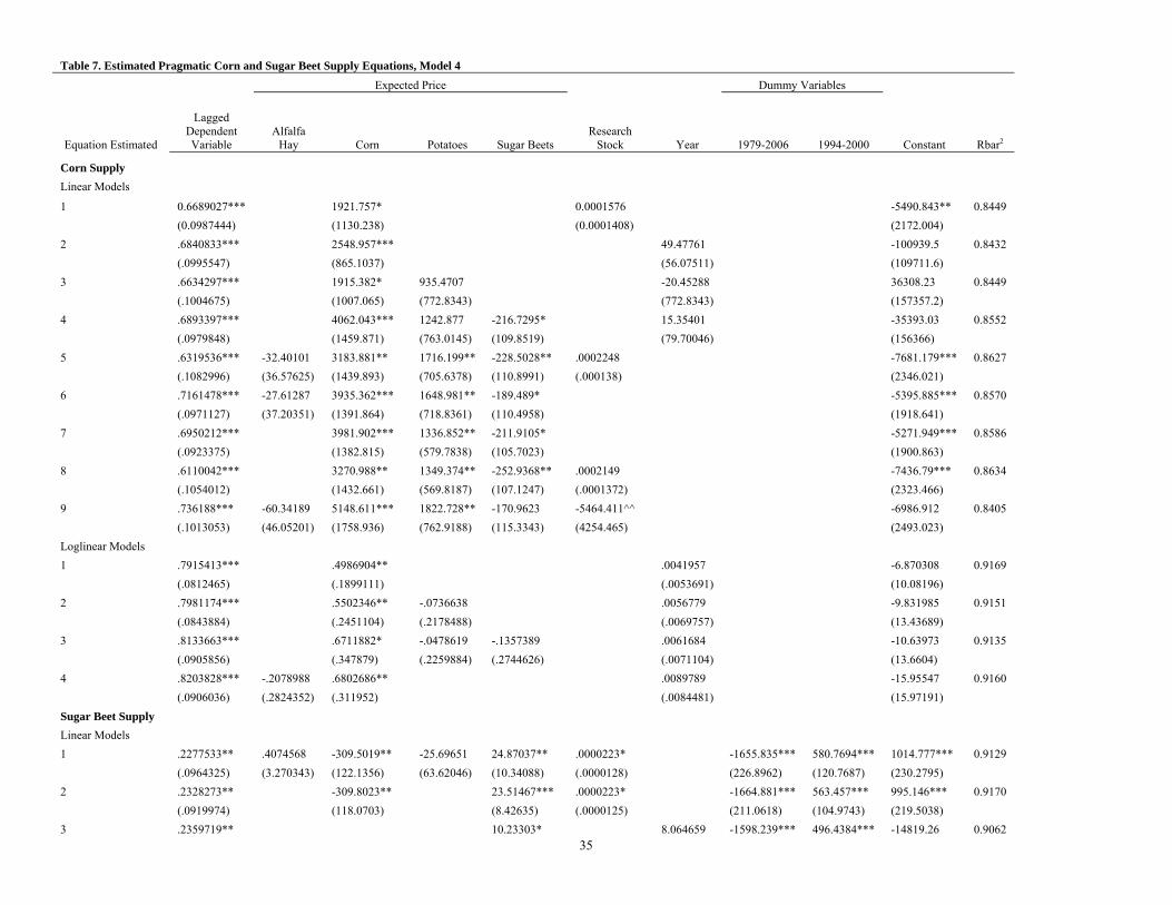
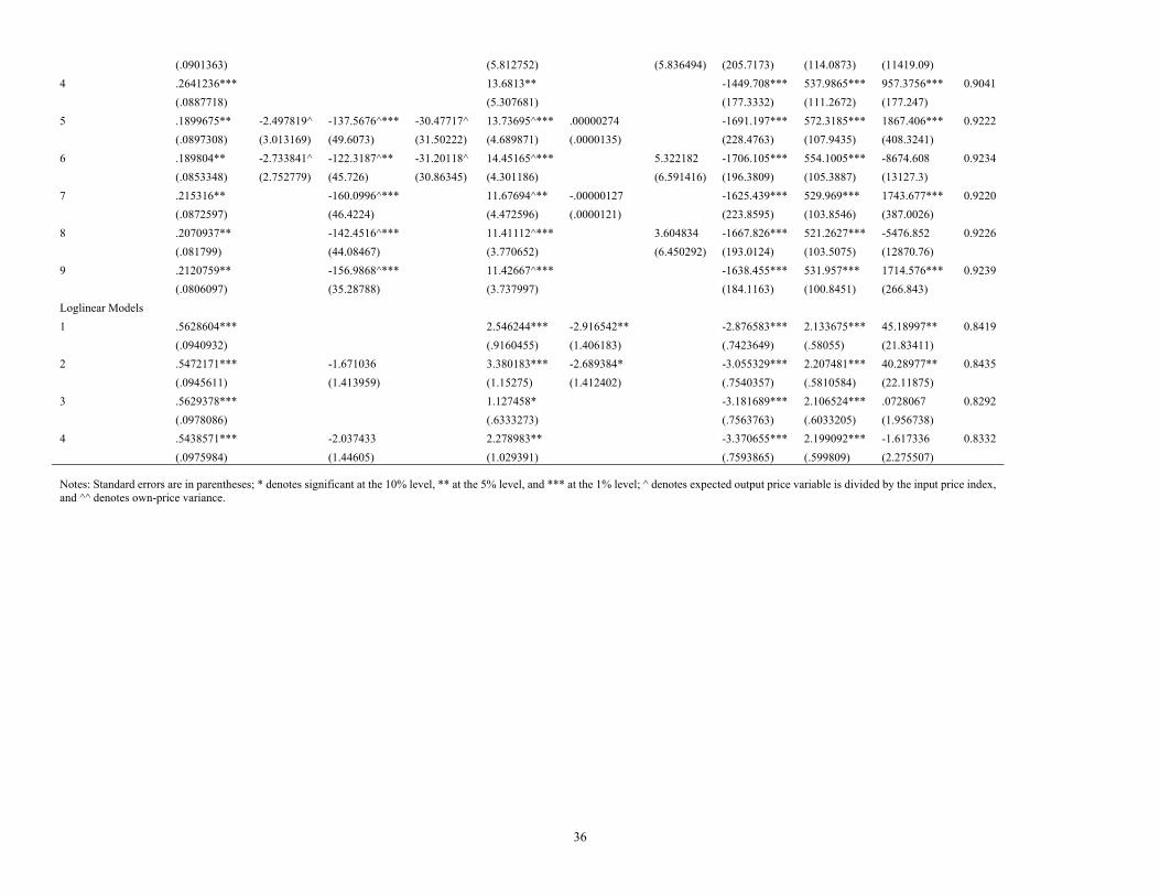
Parameter estimates for other models of corn and sugar beet supply that satisfied the

pragmatic condition are reported in Table 7. In each model reported, both the own-price

coefficient and the coefficient on the lagged dependent variable were significant at the 10% level

and typically at the 5% level. Alfalfa hay price, research stock, and year were never significant in

the corn supply equations. Inclusion of research stock resulted in a higher Rbar2 value in the corn

supply equations, but adding alfalfa hay price consistently lowered it, as did replacing research

stock with year. Functional form had the largest impact on Rbar2 values. Alfalfa hay price, potato

price, and year were never significant in the sugar beet supply equations. Functional form had

the biggest impact on Rbar2 values. All loglinear corn supply equations had higher Rbar2 values

than any of the linear equations, and all linear sugar beet supply equations had higher Rbar2

values than any of the loglinear equations.

Both short-run and long-run own-price elasticity estimates are reported for each of the

pragmatic models in Table 8. For the linear equations, they are computed at the data means.

The estimated elasticities are quite sensitive to model specification, and in the case of sugar beets,

to functional form.

22

The short-run corn supply elasticities vary from 0.46 to 1.22 when computed with the linear

models and from 0.50 to 0.68 when computed with the loglinear models. The average of all

linear models is 0.79 and the average of all loglinear models is 0.60. The elasticity from the

models with highest Rbar2 values is 0.78 for the linear and 0.50 for the loglinear. Since the

loglinear models had consistently and substantially higher Rbar2 values and since Models 1-2 did

not render corn own-price supply elasticities that were both economically meaningful and

statistically significant, we rely mainly on the Model 4 loglinear models for our “best” estimates

of the corn short-run supply elasticity: 0.6 (the loglinear mean) with a possible range from 0.5

(loglinear minimum) to 0.8 (linear mean).

Their long-run elasticities vary between 1.35 and 4.64 from the linear models and between

2.39 and 3.79 from the loglinear models. Averages are 2.54 and 3.13, respectively. Elasticities

from models with highest Rbar2 values are 2.00 and 2.39, respectively. Since the estimates from

models with highest Rbar2 values are lower than either average, we consider them in our best

estimates of the corn long-run supply elasticity: 2.4 (loglinear highest Rbar2) with a possible

range from 2.0 (linear highest Rbar2) to 3.1 (loglinear mean).

The short-run sugar beet elasticities vary from 0.24 to 0.89 when computed with the linear

models and from 1.13 to 3.38 when computed with the loglinear models. The average of all

linear models is 0.62 and the average of all loglinear models is 2.33. The elasticity from the

models with highest Rbar2 values is 0.71 for the linear and 3.38 for the loglinear. Since the linear

models had consistently and substantially higher Rbar2 values, we rely mainly on them and

Model 2 estimates for our best estimates of the sugar beet short-run supply elasticity: 0.7 (linear

highest Rbar2) with a possible range from 0.6 (linear mean) to 1.1 (Model 2 mean and loglinear

minimum).

23

Their long-run elasticities vary from 0.31 to 1.10 from the linear models and from 2.58 to

7.47 from the loglinear models. Averages are 0.79 and 5.22, respectively. Elasticities from

models with highest Rbar2 values are 0.89 and 7.47, respectively. We rely on the linear models

for our best estimate of the sugar beet long-run supply elasticity, 0.9 (linear highest Rbar2), but

consider the lower end of the loglinear range for our upper estimate to provide a possible range

from 0.7 (linear 3rd lowest) to 2.6 (loglinear minimum).

Decision Making and Policy Implications

From these empirical results, we conclude that corn and sugar beets could become

important sources of locally-produced biofuel feedstock in Washington. Sugar beets demonstrate

the largest short-run supply elasticities, so supplies of this crop are expected to show the quickest

response to price or subsidy stimuli. Although current production of Washington sugar beets is

very small, that is due to the lack of a sugar beet processing plant in the State. Washington sugar

beet producers must incur very high transportation costs to get their crop to market. Should

appropriately located ethanol plants be built to handle sugar beets, we might reasonably expect

Washington sugar beet production to quickly return to the levels of the early 1970s.

Although the short-run elasticity estimates for corn are somewhat smaller than for sugar

beets, long-run elasticity estimates are greater. Thus, corn is expected to be more responsive to

price and subsidy stimuli during the 2012-2020 period than sugar beets, so it could become the

more important source of in-state biofuel feedstock with similar economic incentives.

Canola is hard to judge due to the limited quantity produced in the state and the short time

period for which reliable state-level data are available in the U.S. Further, recent production

experience in the State has not been promising (Young 2008). Consequently, we draw no

conclusions about the prospects for this source of in-state biofuel feedstock.

24

Under current legislation, Washington’s Renewable Fuel Standard requires certain licensees

in the fuel production chain to report evidence that at least two percent of gasoline and diesel

sold in the State contain ethanol or biodiesel, respectively, by December 2008 (RCW 19.112.110,

RCW 19.112.120). For example, for a 2.7 billion gallon fuel market, this implies a minimum

requirement of 54 million gallons of biofuel. Currently there is virtually no use of Washington

biomass for biofuel production (Yoder et. al., 2007).

For in-state feedstocks to satisfy the mandated biofuel production demand, a subsidy for

locally produced corn and sugar beets used as biofuel feedstock is likely to generate the quickest

and most visible response from Washington crop producers. Biofuel conversion rates of these

two crops are 0.36 bushel of corn (Lyons 2008) or 80.6 lbs of sugar beets (Salassi, 2007) for a

gallon of ethanol.

Just over 3/4 of the current production of Washington corn or 2/3 of the average production

of Washington sugar beets in the 1970s (with yield increases similar to those in Idaho) would be

sufficient to meet the mandated biofuel production from in-state feedstocks for a 2.7 billion

gallon fuel market (based on Young 2008). Consequently, with ethanol processing facilities

located in appropriate places and capable of utilizing these crops, production that would be

reasonably expected at current prices would be more than sufficient to meet the mandate from

in-state feedstock production. The only incentive needed would be that required to compete with

existing buyers of in-state production of these and competitive crops. Since there is no current

competitor for sugar beets, it is unlikely much of a premium would be required to secure the

entire sugar beet crop for biofuel. For corn, a modest premium may be needed to compete with

current uses of in-state production, but it should not be great. The Washington corn market

reflects the Midwest corn market plus transportation costs, e.g.., average corn price in

25

Washington has averaged 20% higher than the Iowa price during the period 2003-2007.

Assuming that a 10% biofuel feedstock subsidy would be sufficient to secure the entire

Washington corn and sugar beet production for biofuels, they would supply more than 5% of the

total Washington fuel market. To achieve 10% of the current fuel market would require an

estimated additional 120% subsidy in the short run and an estimated 50% subsidy in the long

run.

Conclusions

In this paper, we estimated a wide array of supply equations for three potential biofuel

feedstock crops (corn, sugar beets, and canola) in Washington. We considered a range of models

both for the feedstock crops and for rotational crops. One set of models fully embodied the

theoretical structure implied by expected utility maximization. Other models partially embodied

this framework. Examining the comparative statics results of the models, we conclude that

Washington corn and sugar beets are important potential sources of biofuel feedstock in the State.

Corn is expected to have the greatest potential because it has the largest long-run elasticity, and

the supply can be encouraged by an increase in the market price and/or government subsidy.

Recovery in the sugar beet industry also has significant potential. The potential of canola is less

clear, largely because of data limitations and anecdotal evidence that canola doesn’t compete

well in either current or historical markets with other crops produced in the State.

26

References

Adrangi B. and K. Raffiee. 1999. “On Total Price Uncertainty and the Behavior of a Competitive

Firm.” American Economist 43(2): 59.

Alghalith M. 2007. “Estimation and Econometric Tests under Price and Output Uncertainties.”

Applied Stochastic Models in Business and Industry 23(6): 531-536.

Ball, V.E., C. Hallahan, and R. Nehring. 2004. “Convergence of Productivity: An Analysis of the

Catch-up Hypothesis within a Panel of States,” American Journal of Agricultural

Economics 86:1315-1321.

Chavas J.P. and M. T. Holt. 1990. “Acreage Decisions under Risk: The Case of Corn and

Soybeans.”American Journal of Agricultural Economics 72(3): 529-538.

Chavas J.P. and M. T. Holt. 1996. “Economic Behavior Under Uncertainty: A Joint Analysis of

Risk Preferences and Technology.” The Review of Economics and Statistics 78(2): 329-335.

Coyle B. T. 1992. “Risk Aversion and Price Risk in Duality Models of Production: A Linear

Mean-Variance Approach.” American Agricultural Economics Association 74(4): 849-59.

Huffman, W.E. and R.E. Evenson. 1989. “Supply and Demand Functions for Multiproduct U.S.

Cash Grain Farms: Bias Caused by Research and Other Policies.” American Journal of

Agricultural Economics 71:761-73.

Just R. E. 1974. “An Investigation of the Importance of Risk in Farmers' Decisions.” American

Journal of Agricultural Economics 56(1): 14-25.

Kumbhakar S.C. 2002. “Specification and Estimation of Production Risk, Risk Preferences and

Technical Efficiency.” American Agricultural Economics Association 84(1): 8-22.

Lim, H., and C. R. Shumway. 1992. “Profit Maximization, Returns to Scale, and Measurement

Error.” Review of Economics and Statistics 74(August): 430-38.

27

Lyons, Kim. Biofuels Development in Washington. Washington State University Energy

Extension Program. Olympia, Washington. 2008.

Meyer J., L. J. Robison. “The Aggregate Effects of Risk in the Agricultural Sector.” American

Journal of Agricultural Economics 73(1): 18-24.

Pat Westhoff. 2006. “FAPRI Ethanol Briefing Materials for Congressman Peterson.” Food and

Agricultural Policy Research Institute - University of Missouri Report #02-06.

Pope R. D. 1982. “Empirical Estimation and Use of Risk Preferences: An Appraisal of

Estimation Methods That Use Actual Economic Decisions. American Journal of

Agricultural Economics 64(2): 376-383.

Pope R. D., R. E. Just. 1991. “On Testing the Structure of Risk Preferences in Agricultural

Supply Analysis.” American Journal of Agricultural Economics 73(3): 743-748.

Saha A., C. R. Shumway. 1998. “Refutable implications of the firm model under risk.” Applied

Economics 30: 441-448.

Saha A., C. R. Shumway, H. Talpaz. 1994. “Joint Estimation of Risk Preference Structure and

Technology Using Expo-Power Utility.” American Journal of Agricultural Economics 76(2):

173-184.

Salassi, Michael E. “The Economic Feasibility of Ethanol Production from Sugar Crops.”

Louisiana Agriculture Magazine, Winter, 2007.

Shumway C. R. 1983. “Supply, Demand, and Technology in a Multiproduct Industry: Texas

Field Crops.” American Journal of Agricultural Economics 65(4): 748-760.

U.S. Department of Agriculture/National Agricultural Statistics Service (NASS). 2008. Data and

Statistics. (March). http://www.nass.usda.gov/Data_and_Statistics/Quick_Stats/.

Washington State Biofuels Advisory Committee. 2007. “Implementing the Minimum Renewable

28

Fuel Content Requirements.” (August). http://agr.wa.gov.

Williams S. P., C. R. Shumway. 2000. “Trade Liberalization and Agricultural Chemical Use:

United States and Mexico.” American Agricultural Economics Association 82: 183-199.

Yoder J., P. Wandschneider, et. al. 2007. “Economic Analysis of Market Incentives for Biofuel

Production in Washington State: Interim report to the Governor’s Office and the

Washington State Legislature as directed in E2SSHB 1303 section 402.” Washington State

University, School of Economic Sciences Working Paper.

Young, D. L. 2008. “Feedstock Availability And Economic Potential For Washington State: Crop

Feedstocks.” Washington State University, School of Economic Sciences Working Paper.

Zaikin, A. A., D. L. Young, and W. F. Schillinger. 2008. “Economics of an Irrigated no-till Crop

Rotation with Alternative Stubble Management Systems Versus Continuous Irrigated

Winter Wheat with Burning and Plowing of Stubble, Lind, WA, 2001-2006.” Washington

State University Extension, Farm Business Management Report EB2029E.

29

Table 1. Estimated Washington Corn and Potato Supply Equations, Model 1

Variable/ Parameter Coefficient P-value Supply Elasticity/

Hypothesis Test Value P-value *[ ( )]E Uα π′= 0.43534E-03 0.00000 Corn own-price elasticity -1.2522 0.00000 ˆ( )Uβ π′′= -0.73148E-04 0.00094

1( )pV A -0.68662E-05 0.80580 Corn cross-price

elasticity 0.10005 0.61356 1 1

( )p pV A -0.64870E-04 0.00000

1 2( )p pV A 0.53385E-05 0.62227 Potato own-price

elasticity -0.26488E-01 0.82670 1 1

( )pV Aσ 0.30463E-04 0.28767

1 2( )pV Aσ 0.43084E-04 0.00968 Potato cross-price

elasticity 0.13519E-01 0.62272 1 1

( )pV Aθ 0.59060E-03 0.00000

1 2( )pV Aθ 0.48295E-04 0.25473

Test: Risk Neutrality reject 0.00000 1

( )p wV A 0.14778E-04 0.00004

2( )pV A 0.86937E-03 0.00000 Test: Absence of Output

Price Risk reject 0.01509 2 2

( )p pV A -0.12794E-04 0.80117

2 1( )pV Aσ -0.26175E-03 0.05054 Test: Absence of Output

Quantity Risk reject 0.00000 2 2

( )pV Aσ 0.49174E-04 0.61284

2 1( )pV Aθ -0.88508E-03 0.09245

2 2

( )pV Aθ 0.51741E-03 0.01718

2( )p wV A 0.14541E-03 0.00000

R (research stock) in (13) 0.94984E-05 0.00000

R (research stock) in (14) 0.95870E-06 0.92015

Note: Elasticity estimates are computed at the data means.

30

Table 2. Estimated Washington Sugar beet and Alfalfa Hay Supply Equations, Model 1

Variable/ Parameter Coefficient P-value Supply Elasticity/

Hypothesis Test Value P-value *[ ( )]E Uα π′= 0.45151E-03 0.00000 Sugar beets

own-price elasticity -0.80156 0.18913ˆ( )Uβ π′′= -0.11674E-16 1.00000

1( )pV A 0.14327E-03 0.33228 Sugar beets

cross-price elasticity -0.17798 0.665531 1

( )p pV A -0.35425E-04 0.18760

1 2( )p pV A -0.74118E-05 0.66553 Alfalfa hay own-price

elasticity 0.12125E-01 0.877131 1

( )pV Aσ 0.16287E-03 0.00003

1 2( )pV Aσ -0.22729E-03 0.01008 Alfalfa hay

cross-price elasticity -0.26055E-01 0.665531 1

( )pV Aθ 0.64208E-04 0.59474

1 2( )pV Aθ 0.14685E-03 0.44677

Test: Risk Neutrality reject 0.000041

( )p wV A -0.20230E-04 0.05514

2( )pV A 0.87234E-03 0.00000 Test: Absence of

Output Price Risk reject 0.000022 2

( )p pV A 0.32500E-05 0.87711

2 1( )pV Aσ -0.37749E-05 0.91580 Test: Absence of

Output Quantity Risk not reject 0.511622 2

( )pV Aσ -0.99658E-04 0.13599

2 1( )pV Aθ 0.12593E-04 0.85986

2 2

( )pV Aθ 0.19951E-03 0.08869

2( )p wV A 0.44757E-04 0.00004

R (research stock) in (13) -0.13090E-05 0.90111

R (research stock) in (14) -0.56449E-05 0.47348

d1 (dummy in (14)) 0.35673E-01 0.76151

d2 (dummy in (14)) 0.29244E-03 0.99541

Note: Elasticity estimates are computed at the data means.

31

Table 3. Estimated Washington Corn and Potato Supply Equations, Model 2

Notes: Parameters with a first subscript of 1 are for the corn equation and those with a first

subscript of 2 are for the potatoes equation. Elasticity estimates are computed at the data means.

Parameter (Equation 32)

Risk-Neutral, Profit

Maximization Equations

Expected Utility

Maximization Equations

Coefficient P-value Coefficient P-value

a1 -0.14896 0.16209 -0.29705 0.00018

a11 0.33004E-02 0.07429 0.29662E-18 1.00000

a12 = a21 -0.22401 0.03473 -0.45386E-19 1.00000

a13 0.17062E-04 0.00000 0.19160E-04 0.00000

a2 -0.14982E-01 0.98395 -0.69234 0.37493

a22 543.65 0.16982 0.40257 0.59556

a23 0.83123E-04 0.00000 0.93643E-04 0.00000

b11 — — -1.6811 0.01552

b12 — — 0.32392 0.37042

b13 — — 1.1196 0.12847

b21 — — -14.578 0.00074

b22 — — -1.2982 0.56171

b23 — — 7.0164 0.11724

Corn own price elasticity 0.77742E-02 0.07429 0.69870E-18 1.00000

Corn cross price elasticity -0.42201 0.03473 -0.85502E-19 1.00000

Potatoes own price elasticity 136.41 0.16982 0.10101 0.59556

Potatoes cross price

elasticity -0.70281E-01 0.03473 -0.14239E-19 1.00000

Test: Risk Neutrality — Reject

32

Table 4. Estimated Washington Sugar Beet and Alfalfa Hay Supply Equations, Model 2

Parameter (Equation 32) Risk-Neutral, Profit Maximization

Equations Expected Utility Maximization Equations

Including Variance and Covariance Including Variance Only Coefficient P-value Coefficient P-value Coefficient P-value

a1 0.85988 0.00141 0.76015 0.00069 0.75291 0.00225 a11 0.45892 0.00263 0.51117 0.00260 0.42876 0.01318 a12 = a21 -0.69216E-01 0.64611 -0.19204 0.13270 -0.12772 0.44756 a13 -0.28219E-04 0.00001 -0.21512E-04 0.00024 -0.20604E-04 0.00051 a2 1.7110 0.00000 1.3643 0.00000 1.4506 0.00000 a22 0.15428 0.57433 0.72150E-01 0.41776 0.32772 0.56019 a23 -0.13539E-04 0.34273 0.10263E-04 0.47834 0.40922E-05 0.77288 c1(dummy d1) 0.56646 0.01947 0.29925 0.16532 0.39628 0.11737 c2(dummy d2) 0.83391E-01 0.39049 0.72070E-01 0.42158 0.65700E-01 0.49080 b11 — — 1.2151 0.00003 0.91976 0.00006 b12 — — -2.3310 0.01112 -2.8806 0.00125 b13 — — -1.2529 0.15490 — — b21 — — -0.71506E-02 0.98790 0.27739 0.47141 b22 — — -2.9152 0.00149 -2.7006 0.00785 b23 — — 0.69389 0.42603 — — Sugar beets own-price elasticity 1.0765 0.00263 1.1991 0.00260 1.0058 0.01318 Sugar beets cross-price elasticity -0.15805 0.64611 -0.43852 0.13270 -0.29164 0.44756 Alfalfa hay own-price elasticity 0.57265E-01 0.57433 0.26781E-01 0.41776 0.12164 0.56019 Alfalfa hay cross-price elasticity -0.26394E-01 0.64611 -0.73232E-01 0.13270 -0.48704E-01 0.44756 Test: Risk Neutrality — reject reject

Notes: Parameters with a first subscript of 1 are for the sugar beets equation and those with a first subscript of 2 are for the alfalfa hay equation. Elasticity estimates are computed at the data means.

33

Table 5. Estimated WA, ID, MN, ND Canola and Wheat Supply Equations, Model 3

Parameter

(Equation 35) a Coefficient P-value

Parameter

(Equation 35)a Coefficient P-value

a1WA 0.39165E-01 0.94805 a13MN -0.14670E-05 0.82849

a1ID 0.11538 0.63805 a13ND 0.12348E-03 0.00000

a1MN 0.21275E-01 0.94213 a2WA 2.6953 0.21272

a1ND -2.1296 0.00000 a2ID 1.6460 0.35714

a11WA 0.36786E-16 1.00000 a2MN -1.3603 0.51665

a11ID 0.12869E-15 1.00000 a2ND -4.5965 0.14849

a11MN 0.14722 0.09933 a22WA 1.2474 0.00337

a11ND 0.20243E-14 1.00000 a22ID 0.42298 0.55992

a12WA= a21WA 0.19671E-01 0.78165 a22MN 0.75460 0.33099

a12ID= a21ID -0.39710E-01 0.70158 a22ND 3.2789 0.00000

a12MN= a21MN -0.11191 0.30223 a23WA -0.47670E-04 0.50126

a12ND= a21ND -0.41870 0.00000 a23ID -0.54989E-04 0.60676

a13WA -0.14582E-05 0.94042 a23MN 0.60577E-04 0.22320

a13ID -0.62145E-05 0.67444 a23ND 0.25859E-03 0.04243

Note: Parameters with a first subscript of 1 are from the canola equation, and those with a first subscript of 2 are

from the wheat equation.

34

Table 6. Estimated WA, ID, MN, ND Canola and Wheat Supply Elasticities, Model 3

State Elasticity Value P-value State Elasticity Value P-value

WA

Canola own-price 0.13135E-15 1.00000

MN

Canola own-price 0.49204 0.09933

Canola cross-price 0.48603E-01 0.78165 Canola cross-price -0.31827 0.30223

Wheat own-price 0.11798 0.00337 Wheat own-price 0.82158E-01 0.33099

Wheat cross-price 0.26890E-02 0.78165 Wheat cross-price -0.14318E-01 0.30223

ID

Canola own-price 0.32997E-15 1.00000

ND

Canola own-price 0.63658E-14 1.00000

Canola cross-price -0.96145E-01 0.70158 Canola cross-price -1.1634 0.00000

Wheat own-price 0.39205E-01 0.55992 Wheat own-price 0.34879 0.00000

Wheat cross-price -0.38978E-02 0.70158 Wheat cross-price -0.50405E-01 0.00000

Note: Elasticity estimates are computed at the data means.

35

Table 7. Estimated Pragmatic Corn and Sugar Beet Supply Equations, Model 4 Expected Price Dummy Variables

Equation Estimated

Lagged Dependent Variable

Alfalfa Hay Corn Potatoes Sugar Beets

Research Stock Year 1979-2006 1994-2000 Constant Rbar2

Corn Supply Linear Models

1 0.6689027*** 1921.757* 0.0001576 -5490.843** 0.8449 (0.0987444) (1130.238) (0.0001408) (2172.004) 2 .6840833*** 2548.957*** 49.47761 -100939.5 0.8432 (.0995547) (865.1037) (56.07511) (109711.6) 3 .6634297*** 1915.382* 935.4707 -20.45288 36308.23 0.8449 (.1004675) (1007.065) (772.8343) (772.8343) (157357.2) 4 .6893397*** 4062.043*** 1242.877 -216.7295* 15.35401 -35393.03 0.8552 (.0979848) (1459.871) (763.0145) (109.8519) (79.70046) (156366) 5 .6319536*** -32.40101 3183.881** 1716.199** -228.5028** .0002248 -7681.179*** 0.8627 (.1082996) (36.57625) (1439.893) (705.6378) (110.8991) (.000138) (2346.021) 6 .7161478*** -27.61287 3935.362*** 1648.981** -189.489* -5395.885*** 0.8570 (.0971127) (37.20351) (1391.864) (718.8361) (110.4958) (1918.641) 7 .6950212*** 3981.902*** 1336.852** -211.9105* -5271.949*** 0.8586 (.0923375) (1382.815) (579.7838) (105.7023) (1900.863) 8 .6110042*** 3270.988** 1349.374** -252.9368** .0002149 -7436.79*** 0.8634 (.1054012) (1432.661) (569.8187) (107.1247) (.0001372) (2323.466) 9 .736188*** -60.34189 5148.611*** 1822.728** -170.9623 -5464.411^^ -6986.912 0.8405 (.1013053) (46.05201) (1758.936) (762.9188) (115.3343) (4254.465) (2493.023) Loglinear Models 1 .7915413*** .4986904** .0041957 -6.870308 0.9169 (.0812465) (.1899111) (.0053691) (10.08196) 2 .7981174*** .5502346** -.0736638 .0056779 -9.831985 0.9151 (.0843884) (.2451104) (.2178488) (.0069757) (13.43689) 3 .8133663*** .6711882* -.0478619 -.1357389 .0061684 -10.63973 0.9135 (.0905856) (.347879) (.2259884) (.2744626) (.0071104) (13.6604) 4 .8203828*** -.2078988 .6802686** .0089789 -15.95547 0.9160 (.0906036) (.2824352) (.311952) (.0084481) (15.97191) Sugar Beet Supply Linear Models 1 .2277533** .4074568 -309.5019** -25.69651 24.87037** .0000223* -1655.835*** 580.7694*** 1014.777*** 0.9129 (.0964325) (3.270343) (122.1356) (63.62046) (10.34088) (.0000128) (226.8962) (120.7687) (230.2795) 2 .2328273** -309.8023** 23.51467*** .0000223* -1664.881*** 563.457*** 995.146*** 0.9170 (.0919974) (118.0703) (8.42635) (.0000125) (211.0618) (104.9743) (219.5038) 3 .2359719** 10.23303* 8.064659 -1598.239*** 496.4384*** -14819.26 0.9062

36

(.0901363) (5.812752) (5.836494) (205.7173) (114.0873) (11419.09) 4 .2641236*** 13.6813** -1449.708*** 537.9865*** 957.3756*** 0.9041 (.0887718) (5.307681) (177.3332) (111.2672) (177.247) 5 .1899675** -2.497819^ -137.5676^*** -30.47717^ 13.73695^*** .00000274 -1691.197*** 572.3185*** 1867.406*** 0.9222 (.0897308) (3.013169) (49.6073) (31.50222) (4.689871) (.0000135) (228.4763) (107.9435) (408.3241) 6 .189804** -2.733841^ -122.3187^** -31.20118^ 14.45165^*** 5.322182 -1706.105*** 554.1005*** -8674.608 0.9234 (.0853348) (2.752779) (45.726) (30.86345) (4.301186) (6.591416) (196.3809) (105.3887) (13127.3) 7 .215316** -160.0996^*** 11.67694^** -.00000127 -1625.439*** 529.969*** 1743.677*** 0.9220 (.0872597) (46.4224) (4.472596) (.0000121) (223.8595) (103.8546) (387.0026) 8 .2070937** -142.4516^*** 11.41112^*** 3.604834 -1667.826*** 521.2627*** -5476.852 0.9226 (.081799) (44.08467) (3.770652) (6.450292) (193.0124) (103.5075) (12870.76) 9 .2120759** -156.9868^*** 11.42667^*** -1638.455*** 531.957*** 1714.576*** 0.9239 (.0806097) (35.28788) (3.737997) (184.1163) (100.8451) (266.843) Loglinear Models 1 .5628604*** 2.546244*** -2.916542** -2.876583*** 2.133675*** 45.18997** 0.8419 (.0940932) (.9160455) (1.406183) (.7423649) (.58055) (21.83411) 2 .5472171*** -1.671036 3.380183*** -2.689384* -3.055329*** 2.207481*** 40.28977** 0.8435 (.0945611) (1.413959) (1.15275) (1.412402) (.7540357) (.5810584) (22.11875) 3 .5629378*** 1.127458* -3.181689*** 2.106524*** .0728067 0.8292 (.0978086) (.6333273) (.7563763) (.6033205) (1.956738) 4 .5438571*** -2.037433 2.278983** -3.370655*** 2.199092*** -1.617336 0.8332 (.0975984) (1.44605) (1.029391) (.7593865) (.599809) (2.275507)

Notes: Standard errors are in parentheses; * denotes significant at the 10% level, ** at the 5% level, and *** at the 1% level; ^ denotes expected output price variable is divided by the input price index, and ^^ denotes own-price variance.

37

Lagged Dependent

RegressorsVariable

CoefficientOwn-Price Coefficient Rbar2 Short Run Long Run

Corn Supply:Linear Models1 0.6689027 1921.757 0.8449 0.457 1.3802 .6840833 2548.957 0.8432 0.606 1.9193 .6634297 1915.382 0.8449 0.456 1.3534 .6893397 4062.043 0.8552 0.966 3.1105 .6319536 3183.881 0.8627 0.757 2.0576 .7161478 3935.362 0.8570 0.936 3.2977 .6950212 3981.902 0.8586 0.947 3.1058 .6110042 3270.988 0.8634 0.778 2.0009 .736188 5148.611 0.8405 1.224 4.641 Linear Model Average 0.792 2.540Loglinear Models1 .7915413 .4986904 0.9169 0.499 2.3922 .7981174 .5502346 0.9151 0.550 2.7263 .8133663 .6711882 0.9135 0.671 3.5964 .8203828 .6802686 0.9160 0.680 3.787 Loglinear Model Average 0.600 3.125Sugar Beet Supply:Linear Models1 .2277533 24.87037 0.9129 0.583 0.7552 .2328273 23.51467 0.9170 0.551 0.7193 .2359719 10.23303 0.9062 0.240 0.3144 .2641236 13.6813 0.9041 0.321 0.4365 .1899675 13.73695 0.9222 0.847 1.0466 .189804 14.45165 0.9234 0.891 1.1007 .215316 11.67694 0.9220 0.720 0.9188 .2070937 11.41112 0.9226 0.704 0.8889 .2120759 11.42667 0.9239 0.705 0.894 Linear Model Average 0.618 0.786Loglinear Models1 .5628604 2.546244 0.8419 2.546 5.8252 .5472171 3.380183 0.8435 3.380 7.4653 .5629378 1.127458 0.8292 1.127 2.5804 .5438571 2.278983 0.8332 2.279 4.996 Loglinear Model Average 2.333 5.216

Own-Price Elasticity Estimate

Note: For linear models, elasticities are computed at data means.

Table 8. Own-Price Elasticity Estimates, Pragmatic Models, Model 4