Schema Mappings

Data Exchange &

Metadata Management

Phokion G. Kolaitis IBM Almaden Research Center joint work with Ronald Fagin Renée J. Miller Lucian Popa Wang-Chiew Tan IBM Almaden U. Toronto IBM Almaden UC Santa Cruz

2

The Data Interoperability Problem

n  Data may reside q  at several different sites q  in several different formats (relational, XML, …).

n  Two different, but related, facets of data interoperability:

q  Data Integration (aka Data Federation):

q  Data Exchange (aka Data Translation):

3

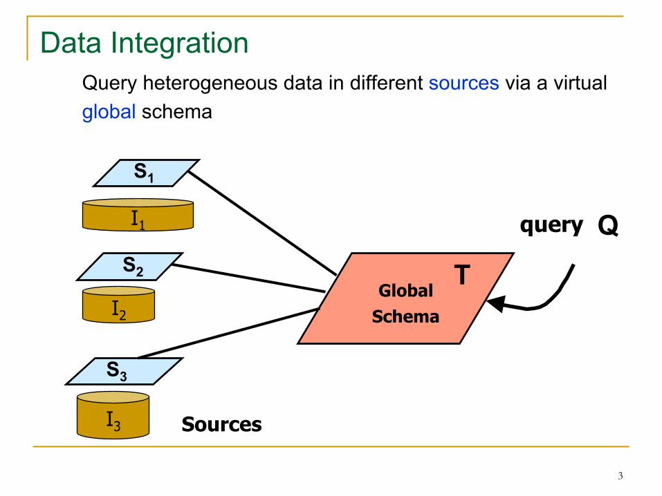
Data Integration Query heterogeneous data in different sources via a virtual global schema

I1

Global Schema I2

I3 Sources

query

S1

S2

S3

T

Q

4

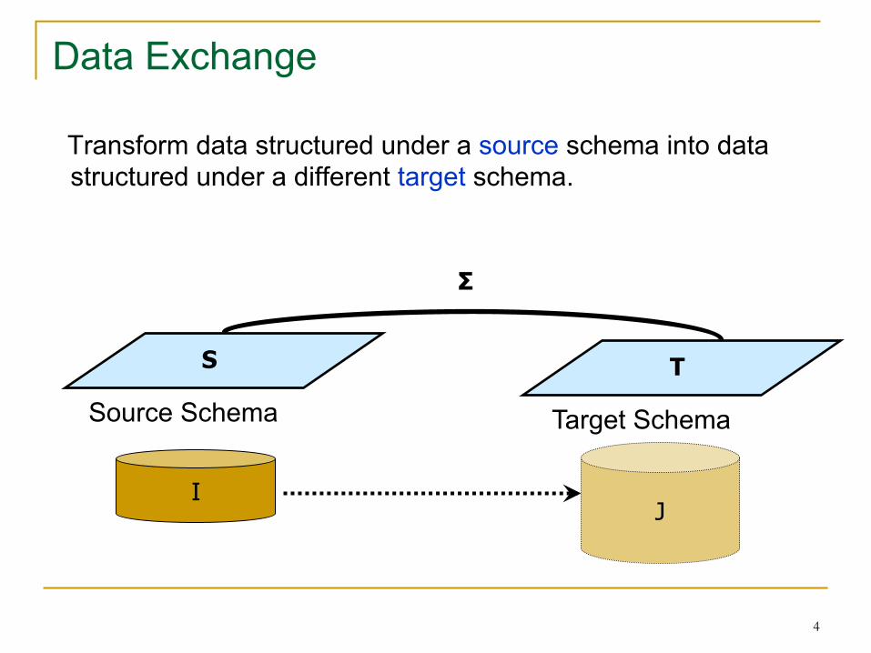
Data Exchange

Transform data structured under a source schema into data structured under a different target schema.

S T

Σ

I J

Source Schema Target Schema

5

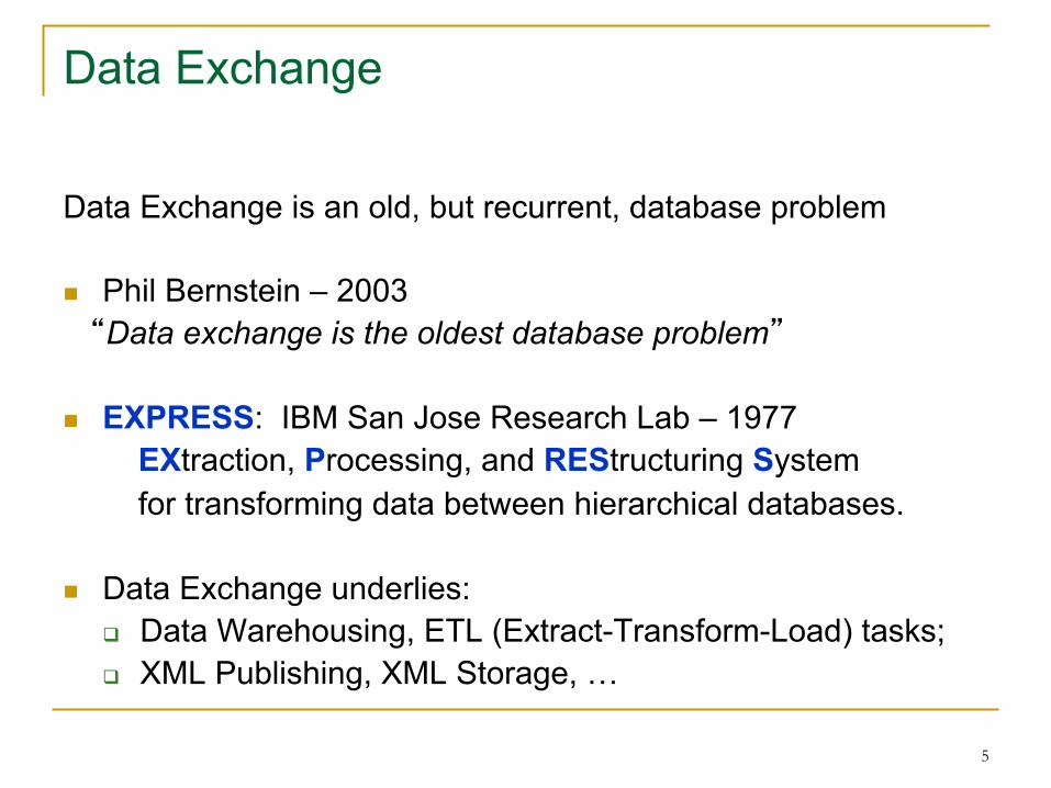
Data Exchange

Data Exchange is an old, but recurrent, database problem n  Phil Bernstein – 2003 “Data exchange is the oldest database problem”

n  EXPRESS: IBM San Jose Research Lab – 1977

EXtraction, Processing, and REStructuring System for transforming data between hierarchical databases.

n  Data Exchange underlies: q  Data Warehousing, ETL (Extract-Transform-Load) tasks; q  XML Publishing, XML Storage, …

6

Foundations of Data Interoperability

Theoretical Aspects of Data Interoperability Develop a conceptual framework for formulating and studying

fundamental problems in data interoperability: n  Semantics of data integration & data exchange n  Algorithms for data exchange n  Complexity of query answering

7

Outline of the Talk

n  Schema Mappings and Data Exchange n  Solutions in Data Exchange

q  Universal Solutions q  The Core of the Universal Solutions

n  Query Answering in Data Exchange n  Composing Schema Mappings

8

Schema Mappings

n  Schema mappings: high-level, declarative assertions that specify the

relationship between two schemas. n  Ideally, schema mappings should be

q  expressive enough to specify data interoperability tasks; q  simple enough to be efficiently manipulated by tools.

n  Schema mappings constitute the essential building blocks in

formalizing data integration and data exchange. n  Schema mappings play a prominent role in Bernstein’s

metadata management framework.

9

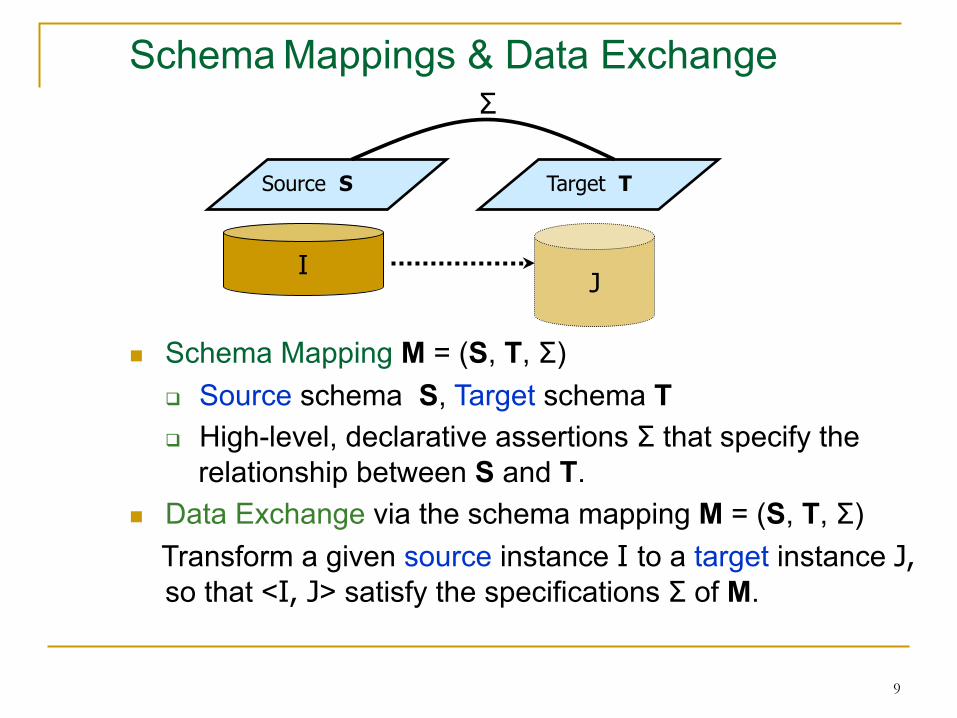
Schema Mappings & Data Exchange

Source S Target T

n  Schema Mapping M = (S, T, Σ) q  Source schema S, Target schema T q  High-level, declarative assertions Σ that specify the

relationship between S and T. n  Data Exchange via the schema mapping M = (S, T, Σ) Transform a given source instance I to a target instance J,

so that <I, J> satisfy the specifications Σ of M.

I J

Σ

10

Solutions in Schema Mappings

Definition: Schema Mapping M = (S, T, Σ) If I is a source instance, then a solution for I is a target instance J such that <I, J > satisfy Σ. Fact: In general, for a given source instance I, q  No solution for I may exist or q  Multiple solutions for I may exist; in fact, infinitely many

solutions for I may exist.

11

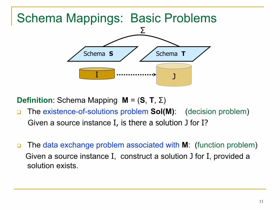
Schema Mappings: Basic Problems

Definition: Schema Mapping M = (S, T, Σ) q  The existence-of-solutions problem Sol(M): (decision problem) Given a source instance I, is there a solution J for I? q  The data exchange problem associated with M: (function problem) Given a source instance I, construct a solution J for I, provided a

solution exists.

Schema S Schema T

I J

Σ

12

Schema Mapping Specification Languages

n  Question: How are schema mappings specified? n  Answer: Use logic. In particular, it is natural to try to use first-order logic as a specification language for schema

mappings. n  Fact: There is a fixed first-order sentence specifying a

schema mapping M* such that Sol(M*) is undecidable. n  Hence, we need to restrict ourselves to well-behaved

fragments of first-order logic.

13

Embedded Implicational Dependencies

n  Dependency Theory: extensive study of constraints in relational databases in the 1970s and 1980s.

n  Embedded Implicational Dependencies: Fagin, Beeri-Vardi, … Class of constraints with a balance between high expressive

power and good algorithmic properties: q  Tuple-generating dependencies (tgds) Inclusion and multi-valued dependencies are a special case. q  Equality-generating dependencies (egds) Functional dependencies are a special case.

14

Data Exchange with Tgds and Egds

n  Joint work with R. Fagin, R.J. Miller, and L. Popa n  Studied data exchange between relational schemas for

schema mappings specified by q  Source-to-target tgds q  Target tgds q  Target egds

15

Schema Mapping Specification Language

The relationship between source and target is given by formulas of first-order logic, called

Source-to-Target Tuple Generating Dependencies (s-t tgds) ϕ(x) → ∃y ψ(x, y), where

§  ϕ(x) is a conjunction of atoms over the source; §  ψ(x, y) is a conjunction of atoms over the target. Example: (Student(s) ∧ Enrolls(s,c)) → ∃t ∃g (Teaches(t,c) ∧ Grade(s,c,g))

16

Schema Mapping Specification Language

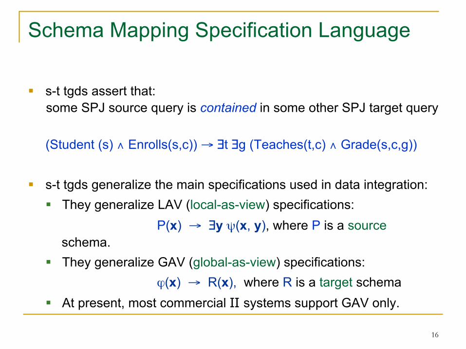
§  s-t tgds assert that: some SPJ source query is contained in some other SPJ target query

(Student (s) ∧ Enrolls(s,c)) → ∃t ∃g (Teaches(t,c) ∧ Grade(s,c,g))

§  s-t tgds generalize the main specifications used in data integration: §  They generalize LAV (local-as-view) specifications: P(x) → ∃y ψ(x, y), where P is a source

schema. §  They generalize GAV (global-as-view) specifications: ϕ(x) → R(x), where R is a target schema §  At present, most commercial II systems support GAV only.

17

Target Dependencies

In addition to source-to-target dependencies, we also consider target dependencies:

q  Target Tgds : ϕT(x) → ∃y ψT(x, y) Dept (did, dname, mgr_id, mgr_name) → Mgr (mgr_id, did) (a target inclusion dependency constraint)

q  Target Equality Generating Dependencies (egds): ϕT(x) → (x1=x2)

(Mgr (e, d1) ∧ Mgr (e, d2)) → (d1 = d2) (a target key constraint)

18

Data Exchange Framework

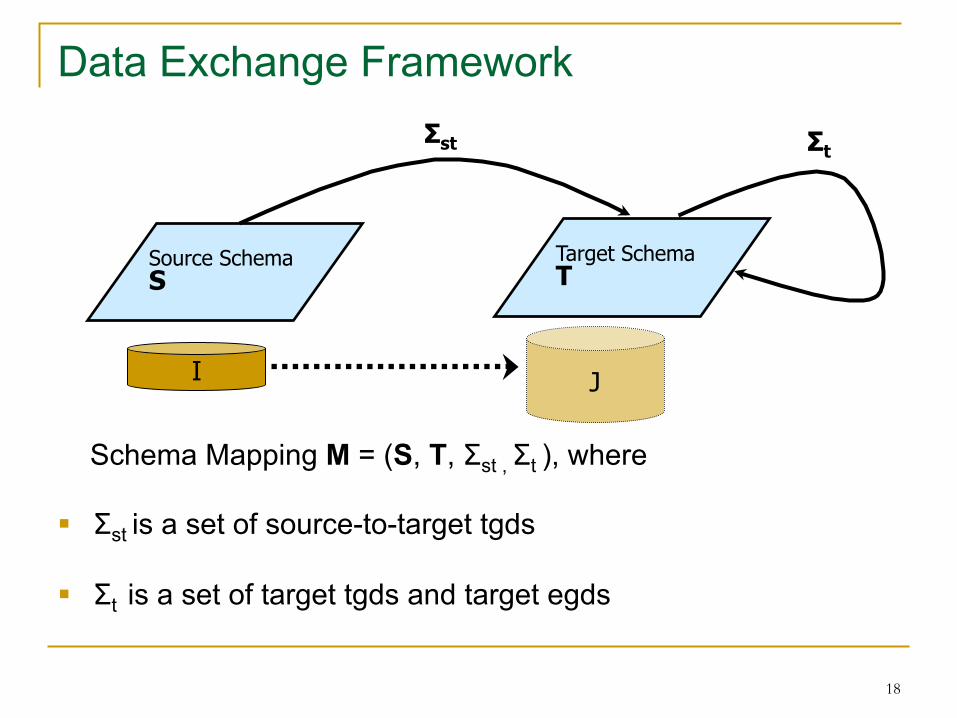
Schema Mapping M = (S, T, Σst , Σt ), where §  Σst is a set of source-to-target tgds

§  Σt is a set of target tgds and target egds

Source Schema S

Target Schema T

Σst

I J

Σt

19

Underspecification in Data Exchange

n  Fact: Given a source instance, multiple solutions may exist. n  Example: Source relation E(A,B), target relation H(A,B) Σ: E(x,y) → ∃z (H(x,z) ∧ H(z,y)) Source instance I = {E(a,b)} Solutions: Infinitely many solutions exist §  J1 = {H(a,b), H(b,b)} constants: §  J2 = {H(a,a), H(a,b)} a, b, … §  J3 = {H(a,X), H(X,b)} variables (labelled nulls): §  J4 = {H(a,X), H(X,b), H(a,Y), H(Y,b)} X, Y, … §  J5 = {H(a,X), H(X,b), H(Y,Y)}

20

Main issues in data exchange

For a given source instance, there may be multiple target instances satisfying the specifications of the schema mapping. Thus,

q  When more than one solution exist, which solutions are

“better” than others? q  How do we compute a “best” solution?

q  In other words, what is the “right” semantics of data exchange?

21

Universal Solutions in Data Exchange

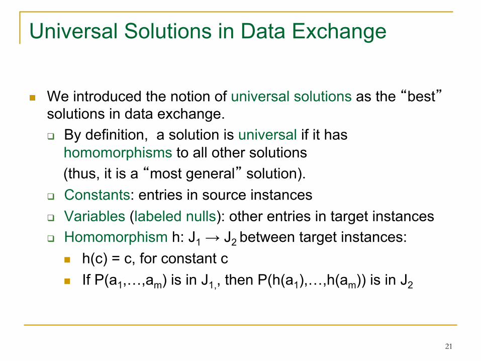
n  We introduced the notion of universal solutions as the “best” solutions in data exchange. q  By definition, a solution is universal if it has

homomorphisms to all other solutions (thus, it is a “most general” solution). q  Constants: entries in source instances q  Variables (labeled nulls): other entries in target instances q  Homomorphism h: J1 → J2 between target instances:

n  h(c) = c, for constant c n  If P(a1,…,am) is in J1,, then P(h(a1),…,h(am)) is in J2

22

Universal Solutions in Data Exchange

Schema S Schema T

I J

Σ

J1 J2

J3

Universal Solution

Solutions

h1 h2 h3 Homomorphisms

23

Example - continued

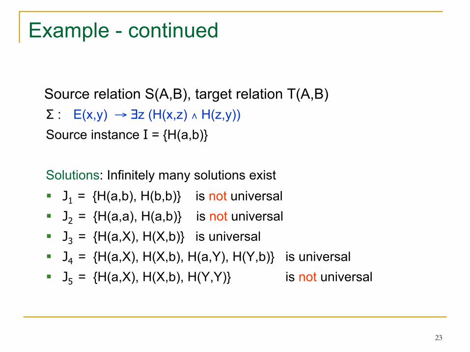
Source relation S(A,B), target relation T(A,B) Σ : E(x,y) → ∃z (H(x,z) ∧ H(z,y)) Source instance I = {H(a,b)} Solutions: Infinitely many solutions exist §  J1 = {H(a,b), H(b,b)} is not universal §  J2 = {H(a,a), H(a,b)} is not universal §  J3 = {H(a,X), H(X,b)} is universal §  J4 = {H(a,X), H(X,b), H(a,Y), H(Y,b)} is universal §  J5 = {H(a,X), H(X,b), H(Y,Y)} is not universal

24

Structural Properties of Universal Solutions

n  Universal solutions are analogous to most general unifiers in logic programming.

n  Uniqueness up to homomorphic equivalence:

If J and J’ are universal for I, then they are homomorphically equivalent.

n  Representation of the entire space of solutions:

Assume that J is universal for I, and J’ is universal for I’. Then the following are equivalent: 1.  I and I’ have the same space of solutions. 2.  J and J’ are homomorphically equivalent.

25

Algorithmic Properties of Universal Solutions

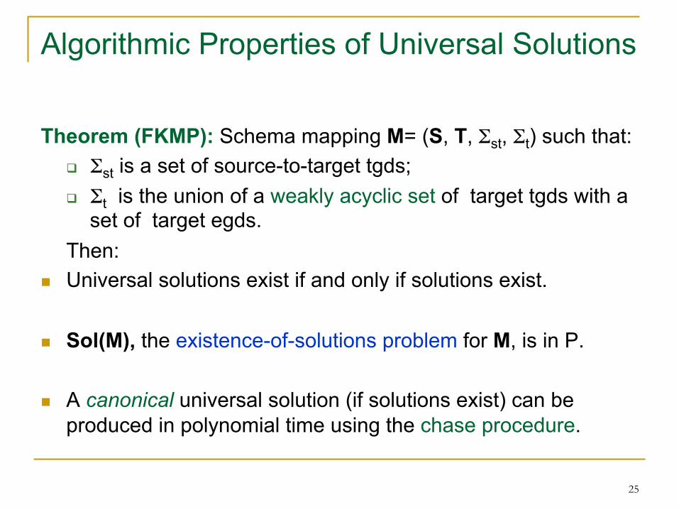
Theorem (FKMP): Schema mapping M= (S, T, Σst, Σt) such that: q  Σst is a set of source-to-target tgds; q  Σt is the union of a weakly acyclic set of target tgds with a

set of target egds. Then:

n  Universal solutions exist if and only if solutions exist.

n  Sol(M), the existence-of-solutions problem for M, is in P. n  A canonical universal solution (if solutions exist) can be

produced in polynomial time using the chase procedure.

26

Weakly Acyclic Sets of Tgds

Weakly acyclic sets of tgds contain as special cases: §  Sets of full tgds ϕT(x) → ψT(x), where ϕT(x) and ψT(x) are conjunctions of target atoms. Example: H(x,z) ∧ H(z,y) → H(x,y) ∧ C(z) Full tgds express containment between relational joins. §  Sets of acyclic inclusion dependencies Large class of dependencies occurring in practice.

27

The Smallest Universal Solution

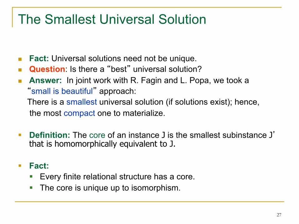
n  Fact: Universal solutions need not be unique. n  Question: Is there a “best” universal solution? n  Answer: In joint work with R. Fagin and L. Popa, we took a “small is beautiful” approach: There is a smallest universal solution (if solutions exist); hence, the most compact one to materialize. §  Definition: The core of an instance J is the smallest subinstance J’

that is homomorphically equivalent to J. §  Fact:

§  Every finite relational structure has a core. §  The core is unique up to isomorphism.

28

The Core of a Structure

J’= core(J)

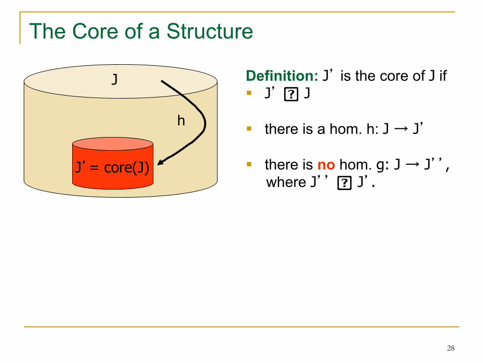
J Definition: J’ is the core of J if §  J’ � J §  there is a hom. h: J → J’ §  there is no hom. g: J → J’’, where J’’ � J’.

h

29

The Core of a Structure

J’= core(J)

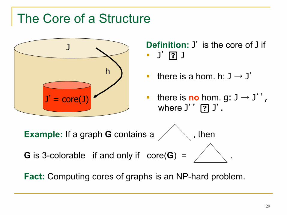
J Definition: J’ is the core of J if §  J’ � J §  there is a hom. h: J → J’ §  there is no hom. g: J → J’’, where J’’ � J’.

h

Example: If a graph G contains a , then G is 3-colorable if and only if core(G) = . Fact: Computing cores of graphs is an NP-hard problem.

30

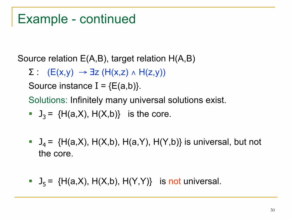
Example - continued

Source relation E(A,B), target relation H(A,B) Σ : (E(x,y) → ∃z (H(x,z) ∧ H(z,y)) Source instance I = {E(a,b)}. Solutions: Infinitely many universal solutions exist. §  J3 = {H(a,X), H(X,b)} is the core. §  J4 = {H(a,X), H(X,b), H(a,Y), H(Y,b)} is universal, but not

the core.

§  J5 = {H(a,X), H(X,b), H(Y,Y)} is not universal.

31

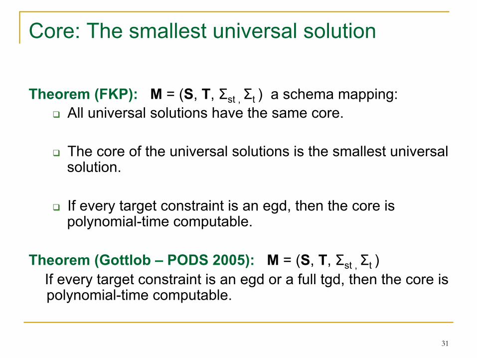
Core: The smallest universal solution

Theorem (FKP): M = (S, T, Σst , Σt ) a schema mapping: q  All universal solutions have the same core. q  The core of the universal solutions is the smallest universal

solution. q  If every target constraint is an egd, then the core is

polynomial-time computable.

Theorem (Gottlob – PODS 2005): M = (S, T, Σst , Σt ) If every target constraint is an egd or a full tgd, then the core is

polynomial-time computable.

32

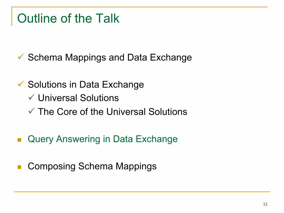
Outline of the Talk

ü  Schema Mappings and Data Exchange

ü  Solutions in Data Exchange ü Universal Solutions ü The Core of the Universal Solutions

n  Query Answering in Data Exchange n  Composing Schema Mappings

33

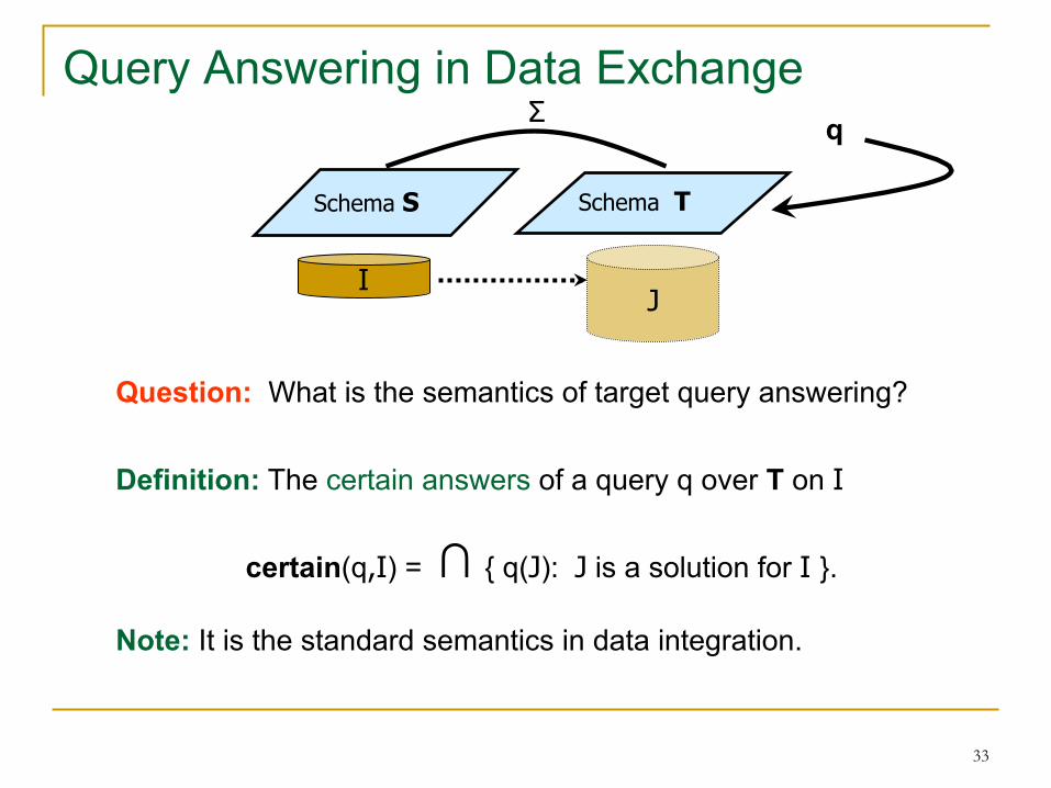
Query Answering in Data Exchange

Schema S Schema T

I J

Σ q

Question: What is the semantics of target query answering?

Definition: The certain answers of a query q over T on I

certain(q,I) = ∩ { q(J): J is a solution for I }. Note: It is the standard semantics in data integration.

34

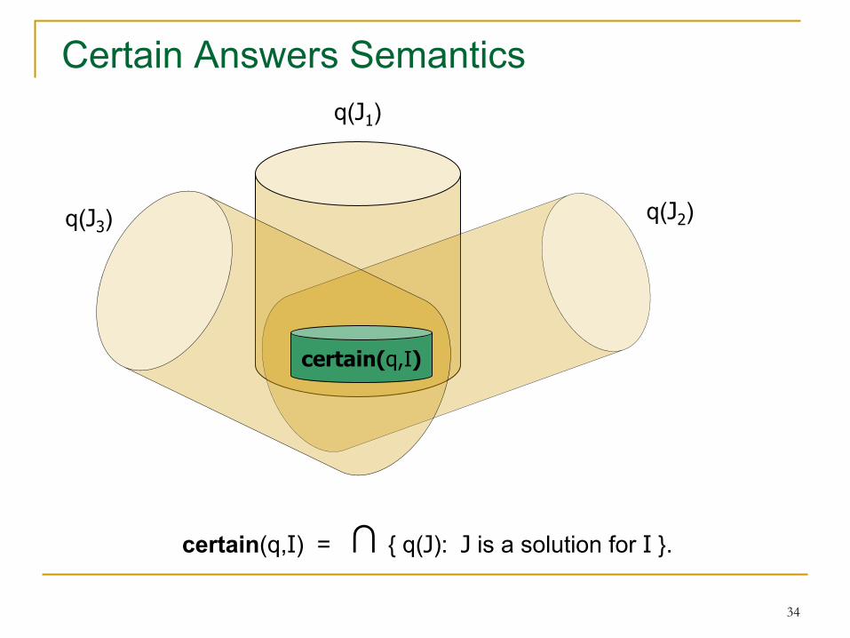
Certain Answers Semantics

certain(q,I)

q(J1)

q(J2) q(J3)

certain(q,I) = ∩ { q(J): J is a solution for I }.

35

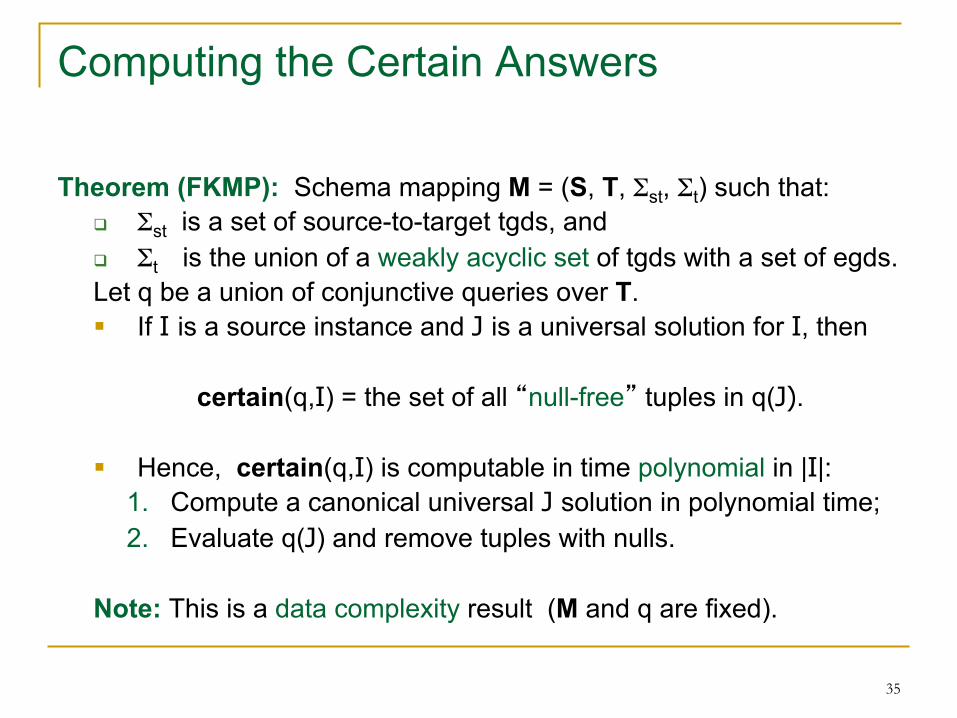
Computing the Certain Answers

Theorem (FKMP): Schema mapping M = (S, T, Σst, Σt) such that: q  Σst is a set of source-to-target tgds, and q  Σt is the union of a weakly acyclic set of tgds with a set of egds. Let q be a union of conjunctive queries over T. §  If I is a source instance and J is a universal solution for I, then certain(q,I) = the set of all “null-free” tuples in q(J). §  Hence, certain(q,I) is computable in time polynomial in |I|:

1.  Compute a canonical universal J solution in polynomial time; 2.  Evaluate q(J) and remove tuples with nulls.

Note: This is a data complexity result (M and q are fixed).

36

Certain Answers via Universal Solutions

q(J1)

q(J2) q(J3)

certain(q,I) = set of null-free tuples of q(J).

q(J) certain(q,I)

q(J)

universal solution J for I

q: union of conjunctive queries

37

Computing the Certain Answers

Theorem (FKMP): Schema mapping M = (S, T, Σst, Σt) such that: q  Σst is a set of source-to-target tgds, and q  Σt is the union of a weakly acyclic set of tgds with a set of egds.

Let q be a union of conjunctive queries with inequalities (�). §  If q has at most one inequality per conjunct, then certain(q,I) is computable in time polynomial in |I| using a disjunctive chase. §  If q is has at most two inequalities per conjunct, then certain(q,I) can be coNP-complete, even if Σt = �.

38

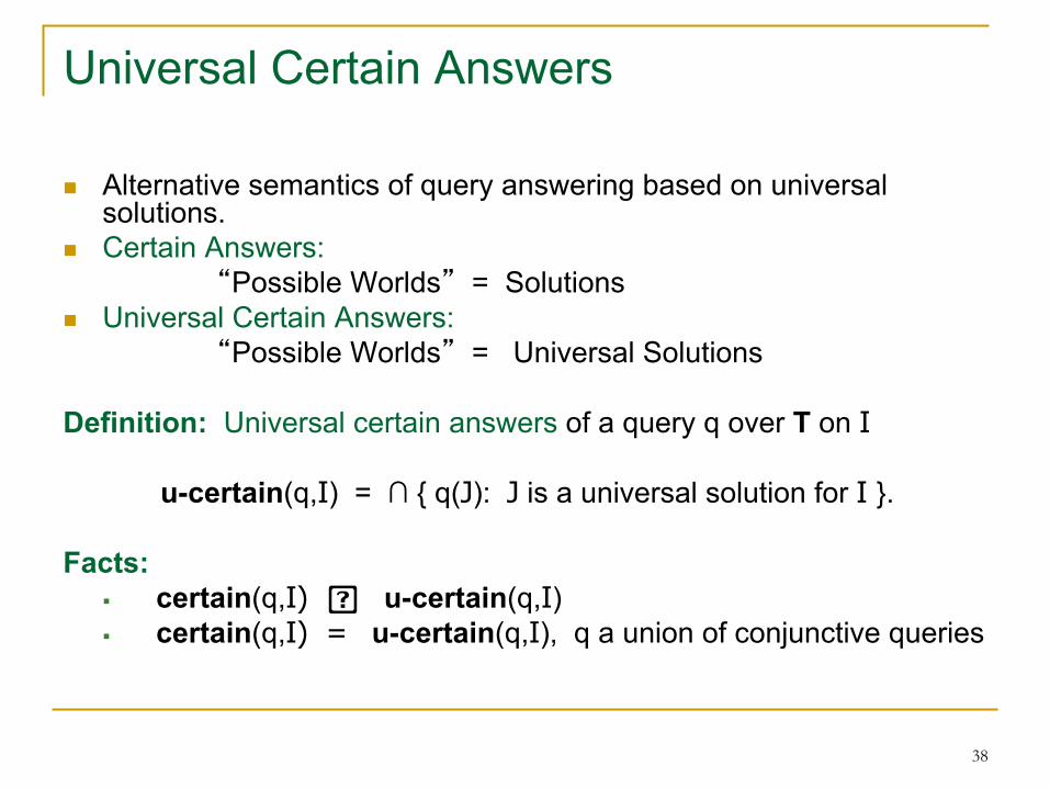
Universal Certain Answers

n  Alternative semantics of query answering based on universal solutions.

n  Certain Answers: “Possible Worlds” = Solutions n  Universal Certain Answers: “Possible Worlds” = Universal Solutions Definition: Universal certain answers of a query q over T on I

u-certain(q,I) = ∩ { q(J): J is a universal solution for I }. Facts:

§  certain(q,I) � u-certain(q,I) §  certain(q,I) = u-certain(q,I), q a union of conjunctive queries

39

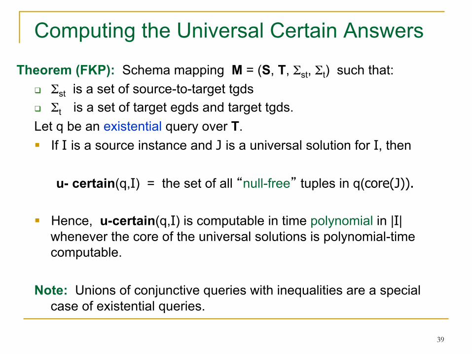
Computing the Universal Certain Answers

Theorem (FKP): Schema mapping M = (S, T, Σst, Σt) such that: q  Σst is a set of source-to-target tgds q  Σt is a set of target egds and target tgds. Let q be an existential query over T. §  If I is a source instance and J is a universal solution for I, then u- certain(q,I) = the set of all “null-free” tuples in q(core(J)). §  Hence, u-certain(q,I) is computable in time polynomial in |I|

whenever the core of the universal solutions is polynomial-time computable.

Note: Unions of conjunctive queries with inequalities are a special

case of existential queries.

40

Universal Certain Answers via the Core

q(J1)

q(J2) q(J3)

u-certain(q,I) = set of null-free tuples of q(core(J)).

q(J) u-certain(q,I)

q(core(J))

universal solution J for I

q: existential

41

From Theory to Practice

n  Clio/Criollo Project at IBM Almaden managed by Howard Ho. q  Semi-automatic schema-mapping generation tool; q  Data exchange system based on schema mappings.

n  Universal solutions used as the semantics of data exchange. n  Universal solutions are generated via SQL queries extended

with Skolem functions (implementation of chase procedure), provided there are no target constraints.

n  Clio/Criollo technology is being exported to WebSphere II.

42

n  Supports nested structures q  Nested Relational

Model q  Nested Constraints

n  Automatic & semi-automatic discovery of attribute correspondence.

n  Interactive derivation of

schema mappings. n  Performs data exchange

Some Features of Clio

43

44

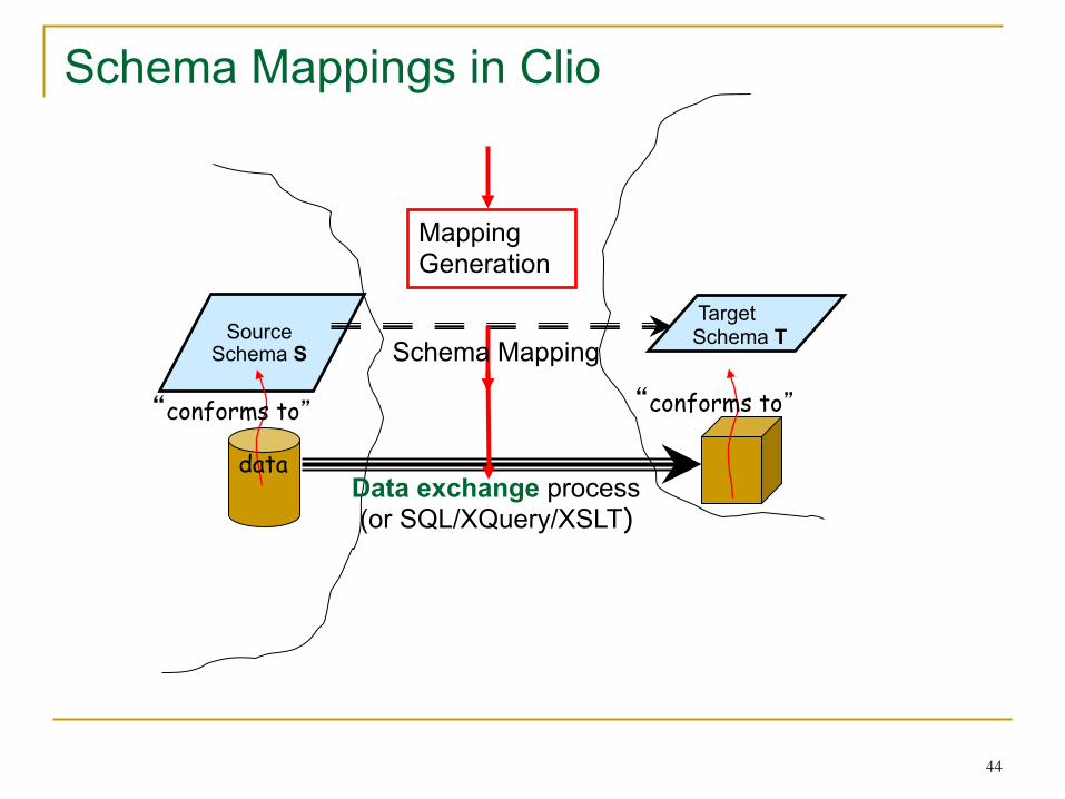
Source Schema S

“conforms to”

data Data exchange process (or SQL/XQuery/XSLT)

“conforms to”

Schema Mappings in Clio

Mapping Generation

Schema Mapping Target Schema T

45

Outline of the Talk

ü  Schema Mappings and Data Exchange

ü  Solutions in Data Exchange ü Universal Solutions ü The Core of the Universal Solutions

ü Query Answering in Data Exchange

n  Composing Schema Mappings joint work with R. Fagin, L. Popa, and W.-C. Tan

46

Managing Schema Mappings

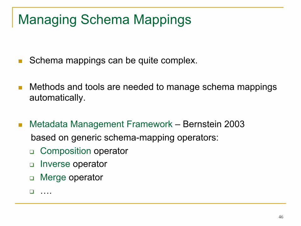
n  Schema mappings can be quite complex.

n  Methods and tools are needed to manage schema mappings automatically.

n  Metadata Management Framework – Bernstein 2003 based on generic schema-mapping operators:

q  Composition operator q  Inverse operator q  Merge operator q  ….

47

Composing Schema Mappings

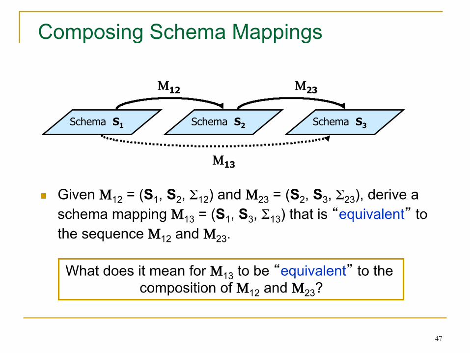
n  Given Μ12 = (S1, S2, Σ12) and Μ23 = (S2, S3, Σ23), derive a schema mapping Μ13 = (S1, S3, Σ13) that is “equivalent” to the sequence Μ12 and Μ23.

Schema S1 Schema S2 Schema S3

Μ12 Μ23

Μ13

What does it mean for Μ13 to be “equivalent” to the composition of Μ12 and Μ23?

48

Earlier Work

n  Metadata Model Management (Bernstein in CIDR 2003) q  Composition is one of the fundamental operators q  However, no precise semantics is given

n  Composing Mappings among Data Sources (Madhavan & Halevy in VLDB 2003)

q  First to propose a semantics for composition q  However, their definition is in terms of maintaining the

same certain answers relative to a class of queries. q  Their notion of composition depends on the class of

queries; it may not be unique up to logical equivalence.

49

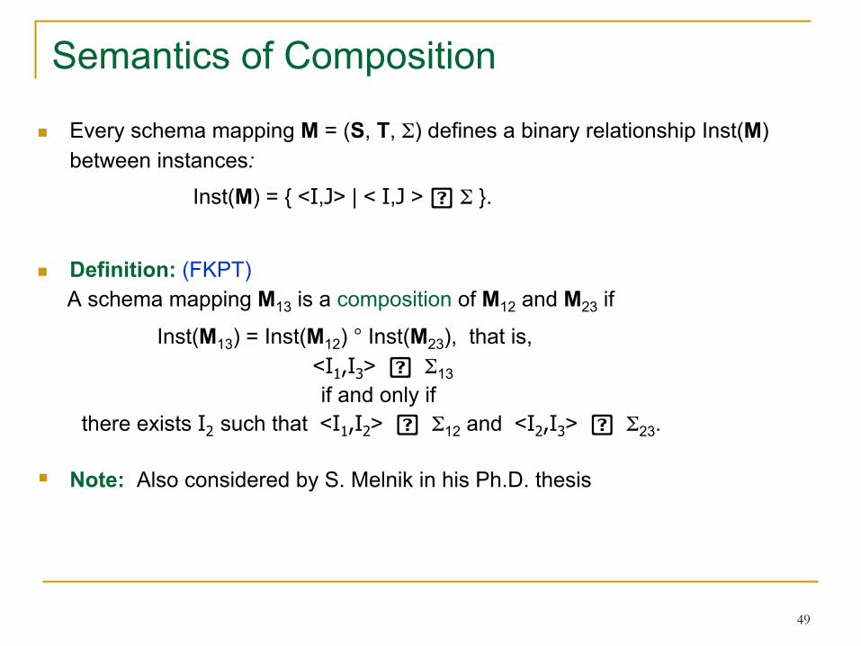
Semantics of Composition

n  Every schema mapping M = (S, T, Σ) defines a binary relationship Inst(M) between instances:

Inst(M) = { <I,J> | < I,J > � Σ }.

n  Definition: (FKPT) A schema mapping M13 is a composition of M12 and M23 if

Inst(M13) = Inst(M12) ° Inst(M23), that is, <I1,I3> � Σ13

if and only if there exists I2 such that <I1,I2> � Σ12 and <I2,I3> � Σ23.

§  Note: Also considered by S. Melnik in his Ph.D. thesis

50

The Composition of Schema Mappings

Fact: If both Μ = (S1, S3, Σ) and Μ’ = (S1, S3, Σ’) are compositions of Μ12 and Μ23, then Σ are Σ’ are logically equivalent. For this reason:

q  We say that Μ (or Μ’) is the composition of Μ12 and Μ23. q  We write Μ12 ° Μ23 to denote it Definition: The composition query of Μ12 and Μ23 is the set

Inst(Μ12) ° Inst(Μ23)

51

Issues in Composition of Schema Mappings

n  The semantics of composition was the first main issue. Some other key issues: n  Is the language of s-t tgds closed under composition? If Μ12 and Μ23 are specified by finite sets of s-t tgds, is Μ12 ° Μ23 also specified by a finite set of s-t tgds? n  If not, what is the “right” language for composing schema

mappings?

52

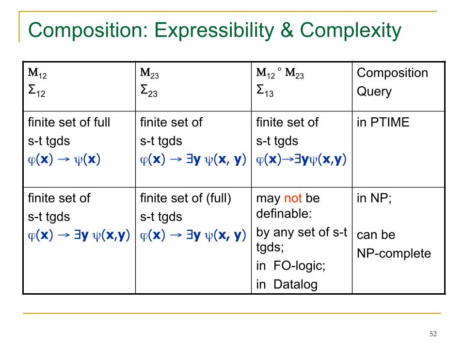
Composition: Expressibility & Complexity

Μ12 Σ12

Μ23 Σ23

Μ12 ° Μ23 Σ13

Composition Query

finite set of full s-t tgds ϕ(x) → ψ(x)

finite set of s-t tgds ϕ(x) → ∃y ψ(x, y)

finite set of s-t tgds ϕ(x)→∃yψ(x,y)

in PTIME

finite set of s-t tgds ϕ(x) → ∃y ψ(x,y)

finite set of (full) s-t tgds ϕ(x) → ∃y ψ(x, y)

may not be definable: by any set of s-t tgds; in FO-logic; in Datalog

in NP; can be NP-complete

53

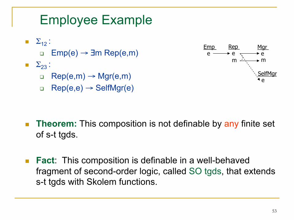
Employee Example n  Σ12 :

q  Emp(e) → ∃m Rep(e,m) n  Σ23 :

q  Rep(e,m) → Mgr(e,m) q  Rep(e,e) → SelfMgr(e)

n  Theorem: This composition is not definable by any finite set

of s-t tgds. n  Fact: This composition is definable in a well-behaved

fragment of second-order logic, called SO tgds, that extends s-t tgds with Skolem functions.

Emp e

Rep e m

Mgr e m

SelfMgr e

54

Employee Example - revisited

Σ12 : q  ∀e ( Emp(e) → ∃m Rep(e,m) )

Σ23 : q  ∀e∀m( Rep(e,m) → Mgr(e,m) ) q  ∀e ( Rep(e,e) → SelfMgr(e) )

Fact: The composition is definable by the SO-tgd Σ13 :

q  ∃f (∀e( Emp(e) → Mgr(e,f(e) ) ∧ ∀e( Emp(e) ∧ (e=f(e)) → SelfMgr(e) ) )

55

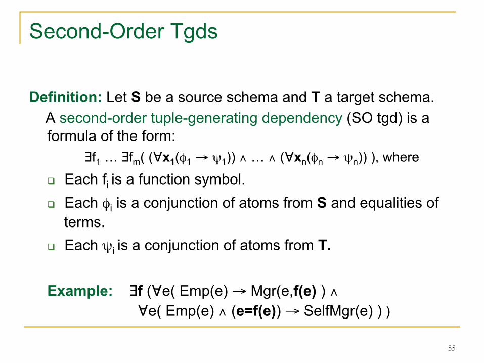
Second-Order Tgds

Definition: Let S be a source schema and T a target schema. A second-order tuple-generating dependency (SO tgd) is a

formula of the form: ∃f1 … ∃fm( (∀x1(φ1 → ψ1)) ∧ … ∧ (∀xn(φn → ψn)) ), where

q  Each fi is a function symbol. q  Each φi is a conjunction of atoms from S and equalities of

terms. q  Each ψi is a conjunction of atoms from T. Example: ∃f (∀e( Emp(e) → Mgr(e,f(e) ) ∧

∀e( Emp(e) ∧ (e=f(e)) → SelfMgr(e) ) )

56

Composing SO-Tgds and Data Exchange

Theorem (FKPT): q  The composition of two SO-tgds is definable by a SO-tgd.

q  There is an algorithm for composing SO-tgds.

q  The chase procedure can be extended to schema mappings specified by SO-tgds, so that it produces universal solutions in polynomial time.

q  For schema mappings specified by SO-tgds, the certain

answers of target conjunctive queries are polynomial-time computable.

57

Synopsis of Schema Mapping Composition

n  s-t tgds are not closed under composition. n  SO-tgds form a well-behaved fragment of second-order logic.

q  SO-tgds are closed under composition; they are a “good” language for composing schema mappings. q  SO-tgds are “chasable”:

Polynomial-time data exchange with universal solutions.

n  SO-tgds and the composition algorithm have been incorporated in Criollo’s Mapping Specification Language (MSL).

58

Related Work and Extensions in this PODS

n  G. Gottlob: Computing Cores for Data Exchange: Algorithms & Practical Solutions

n  A. Nash, Ph. Bernstein, S. Melnik: Composition of Mappings Given by Embedded Dependencies n  A. Fuxman, Ph. Kolaitis, R.J. Miller, W.-C. Tan: Peer Data Exchange n  M. Arenas & L. Libkin: XML Data Exchange: Consistency and Query Answering

59

Theory and Practice

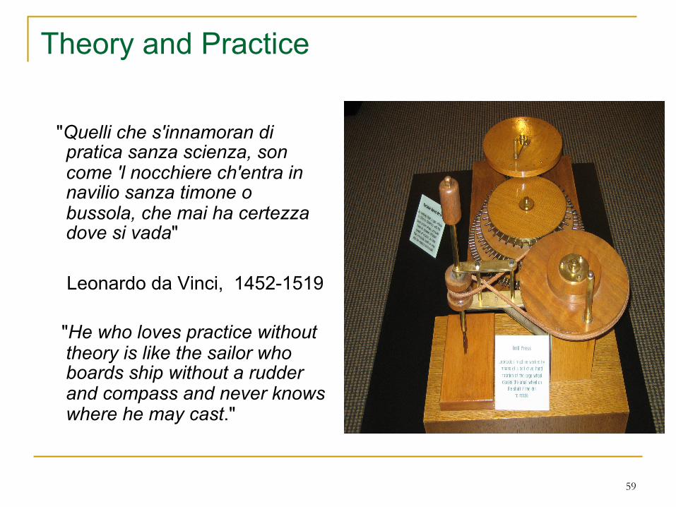
"Quelli che s'innamoran di pratica sanza scienza, son come 'l nocchiere ch'entra in navilio sanza timone o bussola, che mai ha certezza dove si vada"

Leonardo da Vinci, 1452-1519 "He who loves practice without

theory is like the sailor who boards ship without a rudder and compass and never knows where he may cast."

60

Reduction from 3-Colorability

n  Σ12 q  ∀x∀y (E(x,y) → ∃u∃v (C(x,u) ∧ C(y,v))) q  ∀x∀y (E(x,y) → F(x,y))

n  Σ23 q  ∀x∀y∀u∀v (C(x,u) ∧ C(y,v) ∧ F(x,y) → D(u,v))

n  Let I3 = { (r,g), (g,r), (b,r), (r,b), (g,b), (b,g) }

n  Given G=(V, E), q  let I1 be the instance over S1 consisting of the edge relation E

of G

n  G is 3-colorable iff <I1,I3> ∈ Inst(Μ12) ° Inst(Μ23)

n  [Dawar98] showed that 3-colorability is not expressible in L∞ω ω

61

Algorithm Compose(Μ12, Μ23)

n  Input: Two schema mappings Μ12 and Μ23 n  Output: A schema mapping Μ13 = Μ12° Μ23

n  Step 1: Split up tgds in Σ12 and Σ23 q  C12 = Emp(e) → (Mgr1(e, f(e)) q  C23 =

n  Mgr1(e,m) → Mgr(e,m) n  Mgr1(e,e) → SelfMgr(e)

n  Step 2: Compose C12 with C23

q  χ1 : Emp(e0) ∧ (e=e0) ∧ (m=f(e0)) → Mgr1(e,m) q  χ2 : Emp(e0) ∧ (e=e0) ∧ (e=f(e0)) → SelfMgr(e)

n  Step 3: Construct Μ13 q  Return Μ 13 = (S1, S3, Σ13) where q  Σ13 = ∃f(∃e0 ∃e∃m χ1 ∧ ∃e0∃e χ2)