scheduling unrelated parallel machines with resource … unrelated parallel machines with...

Scheduling unrelated parallel machines with

resource-assignable sequence dependent setup times

Rubén Ruiz1∗, Carlos Andrés2

1 Grupo de Sistemas de Optimización Aplicada, Instituto Tecnológico de Informática,

Universidad Politécnica de Valencia, Valencia, Spain. [email protected]

2Departamento de Organización de Empresas,

Universidad Politécnica de Valencia, Valencia, Spain. [email protected].

January 28, 2007

Abstract

A novel scheduling problem that results from the addition of resource-assignable

setups is presented in this paper. We consider an unrelated parallel machine problem

with machine and job sequence dependent setup times. The new characteristic is that

the amount of setup time do not only depend on the machine and job sequence, but

also on a number of resources assigned, which can vary between a minimum and a

maximum. The aim is to give solution to real problems arising in several industries

where frequent setup operations in production lines have to be carried out. These

operations are indeed setups whose length can be reduced or extended according

to the number of resources assigned to them. The objective function considered

is a linear combination of total completion time and the total number of resources

assigned. We present a MIP model and some fast dispatching heuristics. We carry

out careful and comprehensive statistical analyses to study what characteristics of

the problem affect the MIP model performance. We also study the effectiveness of

the different heuristics proposed.

Keywords: scheduling, unrelated parallel machines, sequence dependent setups, total

completion time, resources

∗Corresponding author. Tel: +34 96 387 70 07, ext: 74946. Fax: +34 96 387 74 99

1

1 Introduction

Parallel machine scheduling problems contain an interesting number of characteristics that set

them aside in the scheduling field. In these problems, there is a set N = 1, 2, . . . , n of jobs where

each one has to be processed exactly on one machine from the set M = 1, . . . ,m. Firstly, jobs have

to be assigned to machines and secondly, among the jobs assigned to each machine, a processing

sequence must be derived. Among parallel machine scheduling problems, the most general case

is when the parallel machines are said to be unrelated. In this scenario, the processing time of

each job depends on the machine to which it is assigned. This processing time is deterministic

and known in advance and is denoted by pij, i ∈ M , j ∈ N .

In this paper we are interested in a complex and realistic variant of the unrelated parallel machine

scheduling problem. We consider machine and sequence dependent setup times which can be

separated from processing times. A setup is a non-productive period of time which usually

modelizes operations to be carried out on machines after processing a job to leave them ready for

processing the next job in the sequence. Therefore, Sijk is the setup time to be carried out on

machine i after having processed job j and before processing job k, i ∈ M , j, k ∈ N, j 6= k. Setup

times frequently represent cleaning production lines and/or adding/removing elements from a

line when changing from one type of job to another. A clear example stems from the ceramic tile

manufacturing sector. At the glazing stage there are several unrelated parallel lines (machines)

capable of glazing the different types of ceramic tile lots (jobs). After glazing a lot, the glazing

line needs to be cleaned and prepared for the glazing of the next lot or job. This is the setup time

which clearly depends on the line type and on the processing sequence. Modern glazing lines are

easier to clean whereas old and end-of-life lines need more careful cleaning. Additionally, if the

last tile lot glazed had a strong color, a much more time consuming cleaning must be carried

out, specially if the next tile lot has a clear color. Hence, setup times are machine and sequence

dependent.

Sijk is difficult to set in practice. One of the reasons is that if more resources are devoted to a

given setup operation, the setup time decreases. In the previous ceramic tile example, resources

are usually cleaning machinery and/or plant personnel. The cleaning of the glazing line might

take several hours if a single person is carrying out the cleaning. However, if several workers clean

the line, the setup time decreases. In this paper, apart from the machine and sequence dependent

setup times, we also consider the resources assigned to each setup, which affect the time the setup

needs. We will denote by Rijk the amount of resources devoted to carrying out setup Sijk. We refer

to this as resource-assignable sequence dependent setup times or RASDST in short. Obviously,

assigning more resources would certainly reduce the total setup time. However, such resources

are usually costly and a trade-off situation arises. Consequently, we are interested in a realistic

optimization criterion which minimizes the total production time or flowtime. If we denote by

Cj the completion time of job j at the shop, the total completion time or flowtime is given by∑n

j=1 Cj . Is is well known that minimizing flowtime minimizes as well cycle time and maximizes

2

throughput. All these measures are very important in practice. Of course, the total resource

assignment must be considered. We denote by TRes the total number of resources assigned to

setups (i.e., TRes =∑m

i=1

∑nj=1

∑nk=1,k 6=j Rijk). Additionally, given α and β that modelize the

importance or cost of each unit of resource and flowtime, respectively, the objective function

considered in this paper is αTRes + β∑n

j=1 Cj, where α, β ≥ 0. Such a problem, that can be

denoted as R/Sijk, Rijk/αTRes +β∑n

j=1 Cj by extending the the notation given in Graham et al.

(1979) is obviously NP-Hard. The unrelated parallel machine problem without setups and total

completion time criterion (R//∑n

j=1 Cj) is in P according to Horn (1973) where the optimum

solution can be simply derived with the Shortest Processing Time rule (SPT). However, the case

where the parallel machines are identical and there are only sequence independent family setup

times, i.e., the problem P/Sj/∑n

j=1 Cj is already NP-Hard as explained in Webster (1997).

Therefore, by simple reduction to this problem, the unrelated parallel machines problem with

resource-assignable sequence dependent setup times tackled in this paper is also NP-Hard. As a

result, heuristics are the only alternative for realistically-sized problems.

In Section 2 we review the literature of related problems, since, as we will show and to the best

of our knowledge, the problem tackled in this paper has not been addressed in the literature

before. Due to its novelty, a MIP model for obtaining the exact solution is presented in Section 3,

along with a more detailed notation of the problem. Section 4 presents some static and dynamic

dispatching heuristics for the problem, along with an exact rule for assigning setup resources,

once the job assignment to machines and processing sequence is given. A complete testing and

evaluation of both the MIP model as well as the heuristics is given in Section 5. Comprehensive

statistical analyses help supporting the results. Lastly, some conclusions and further research

topics are presented in Section 6.

2 Literature review

In the literature there are several reviews and surveys about scheduling with setup times like the

ones of Yang and Liao (1999), Allahverdi et al. (1999) and more recently, Allahverdi et al. (2007).

There are also specific surveys dealing with parallel machine settings like those of Cheng and Sin

(1990), Lam and Xing (1997) and Mokotoff (2001). A careful examination of these reviews results

in no paper dealing with the problem considered in this work.

From our perspective, unrelated parallel machine problems with sequence dependent setup times

contain the principal characteristics of the problem studied here and therefore we focus the re-

view mainly on them. Some of the earlier studies come from Marsh and Montgomery (1973)

where problems with identical as well as unrelated parallel machines and sequence dependent

setup times are considered. The objective function is the minimization of total setups. Guinet

(1991) considered the unrelated machines case also with sequence and machine dependent setups.

Heuristics and mathematical modeling were employed to solve the mean tardiness and mean com-

3

pletion time criteria. In a later paper, Guinet and Dussauchoy (1993) study the same problem

but in this case with identical parallel machines and makespan as well as mean completion time

criteria. The authors develop some routing-based heuristics as solution methods. Lee and Pinedo

(1997) propose a three-phase heuristic also for the identical machine problem but in this case for a

total weighted tardiness criterion. Most literature deals with the identical parallel machine prob-

lem and finding results for the unrelated machine case with sequence dependent setup times is

difficult. For example, the papers of Balakrishnan et al. (1999), Sivrikaya-Serifoglu and Ulusoy

(1999), or Radhakrishnan and Ventura (2000) propose different techniques for the identical or

uniform parallel machine problems with sequence dependent setup times and using different ear-

liness and tardiness criteria. There are, however, some exceptions. In Zhu and Heady (2000), a

mixed integer programming model is proposed for the unrelated machines, sequence dependent

setup problem with earliness/tardiness objective. Weng et al. (2001) study the same problem

but with two differences: the criterion studied is the mean completion time and the setup times

depend only on the job sequence and not on the machine. The authors propose seven dispatching

heuristics for the problem and compare the results in comprehensive experiments. A similar prob-

lem is dealt with in Kim et al. (2002) but with total tardiness criterion and with the additional

characteristic that jobs are grouped into families and the setups are family-based. More recently,

Rabadi et al. (2006) have proposed several GRASP-like heuristics for an unrelated machines case

with machine and job sequence dependent setup times with makespan criterion.

As we can see, to the best of our knowledge, no scheduling problem has been studied in the

literature where the setup times can be resource-assignable. However, there is a large body of

literature where the processing times can be controlled. A good review of these types of problems

is given by Nowicki and Zdrzalka (1990). In these cases, processing time can be controlled or

“compressed” at a given cost. The closest reference we find is due to Zhang et al. (2001) where an

unrelated parallel machine problem with controllable processing times is examined. In this case,

the objective considered in a combination of total weighted completion time and total processing

time compression costs. However, no setup times are considered. Lastly, we find an interesting

reference due to Chen (2006), where a complex problem from the semiconductor industry is ap-

proached. The problem resembles an unrelated parallel machine setting with tooling mounting

and un-mounting at the machines. This mounting operations can be seen as sequence-independent

setups. The interesting fact is that although the setup times are fixed, a given resource is needed

for each setup.

The conclusion from this review is that the complex unrelated parallel machine with resource-

assignable machine and job sequence dependent setup times problem considered in this paper is

novel. To the best of our knowledge, this problem has not been considered before in the literature.

4

3 Problem and MIP model formulation

Now we give further notation and definitions for the unrelated parallel machine RASDST problem.

For each possible setup time Sijk we have a set of four values. The first two specify the minimum

and maximum quantities of resources that can be assigned to each setup. Therefore, R−ijk(R

+ijk)

denote the minimum (maximum) resources assignable to setup Sijk. Let us consider again the

ceramic tile glazing lines example of Section 1. Some setups might require removing certain heavy

tooling from the glazing lines and therefore a minimum amount of workers (resources) are needed.

Similarly, at a given moment it might not be possible to assign more resources due to physical or

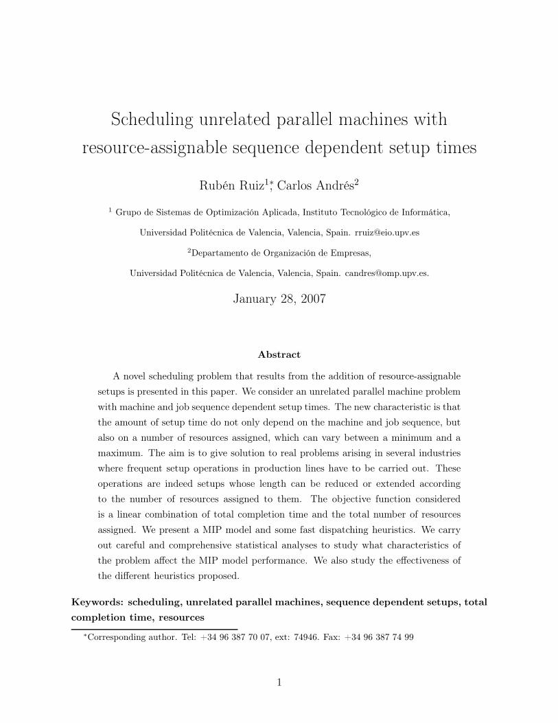
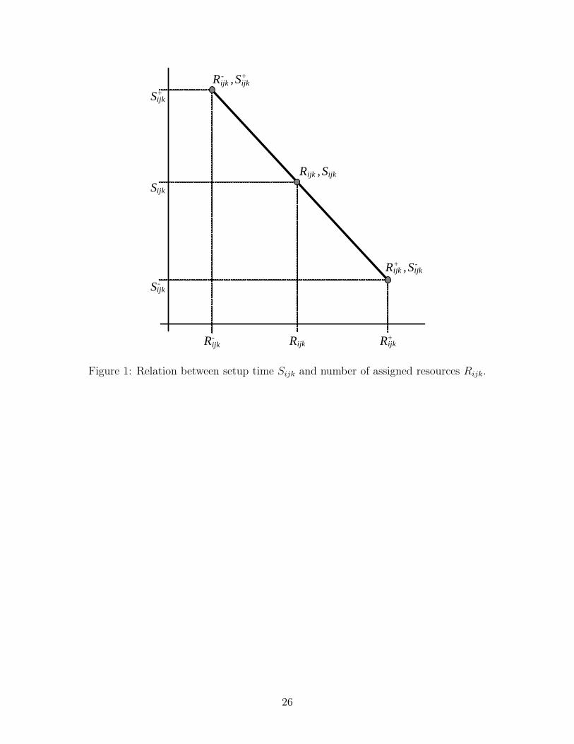
operational constraints. The relation between the actual setup time and the number of resources

assigned is assumed in this work to be linear. Therefore, if the minimum resources R−ijk

are

assigned, the resulting setup time will be the largest possible, denoted as S+ijk

. Conversely, if the

maximum resources are assigned, R+ijk, the setup will be minimum (S−

ijk). This relation is shown

in Figure 1.

[Insert Figure 1 about here]

Therefore, from the linear relation, the expression that returns the amount of setup time Sijk as

a function of the assigned resources Rijk is the following:

Sijk = S+ijk −

S+ijk − S−

ijk

R+ijk − R−

ijk

(Rijk − R−ijk) = S+

ijk +S+

ijk − S−ijk

R+ijk − R−

ijk

R−ijk −

S+ijk − S−

ijk

R+ijk − R−

ijk

Rijk (1)

Using K1 and K2 for the first terms and for the Rijk multiples, respectively we have as a result

the slope-intercept form of the line relating Sijk and Rijk:

Sijk = K1 − K2Rijk (2)

Therefore, K2 is the slope of the line that relates Rijk with Sijk as shown in Figure 1. In

other words, K2 indicates how much the setup time Sijk is reduced by each additional re-

source. For example, given S+ijk = 20, S−

ijk = 4, R+ijk = 10 and R−

ijk = 2 we would have

Sijk = 20 − 20−410−2 (Rijk − 2) = 24 − 2Rijk. As a result, each additional resource would decrease

the setup time in two units.

With the definition of the setup times we can now derive a mathematical mixed integer pro-

gram (MIP) to obtain the optimum solution of the unrelated parallel machine RASDST problem.

The model uses the following decision variables:

5

Xijk =

{

1, if job j precedes job k on machine i

0, otherwise

Cij = Completion time of job j at machine i

Rijk = Resources assigned to the setup between job j and job k on machine i

The objective function is:

min∑

i∈M

∑

j∈N

∑

k∈Nk 6=j

αRijk +∑

i∈M

∑

j∈N

βCij (3)

And the constraints are:∑

i∈M

∑

j∈{0,N}j 6=k

Xijk = 1, k ∈ N (4)

∑

i∈M

∑

k∈Nj 6=k

Xijk ≤ 1, j ∈ N (5)

∑

k∈N

Xi0k ≤ 1, i ∈ M (6)

∑

h∈{0,N}h 6=k,h 6=j

Xihj ≥ Xijk, j, k ∈ N, j 6= k, i ∈ M (7)

Cik + V (1 − Xijk) ≥ Cij + K1 − K2Rijk + pik, j ∈ {0, N}, k ∈ N, j 6= k, i ∈ M (8)

Rijk ≥ R−ijk

, j, k ∈ N, j 6= k, i ∈ M (9)

Rijk ≤ R+ijk

, j, k ∈ N, j 6= k, i ∈ M (10)

Ci0 = 0, i ∈ M (11)

Cij ≥ 0, j ∈ N, i ∈ M (12)

Xijk ∈ {0, 1}, j ∈ {0, N}, k ∈ N, j 6= k, i ∈ M (13)

The objective minimizes a linear combination of the total resources assigned (TRes) and the total

completion time. Constraint set (4) ensures that every job has exactly one predecessor. Notice

the usage of dummy jobs 0 as Xi0k, i ∈ M,k ∈ N . Conversely, constraint set (5) limits the

number of successors of every job to one. Set (6) limits the number of successors of the dummy

jobs to a maximum of one on each machine, i.e., dummy job 0 can have at most one successor

on each machine. With set (7) we ensure that jobs are properly linked in machines since if a

given job j is processed o a given machine i, it must have a predecessor h on the same machine.

Constraint set (8) is central for controlling the completion times of the jobs at the machines.

Basically, if a job k is assigned to machine i after job j (i.e., Xijk = 1), its completion time Cik

6

must be greater than the completion time of j, Cij plus the setup time between j and k and the

processing time of k. Notice how the setup time is expressed here according to equation (2). If

Xijk = 0, then the big constant V renders the constraint redundant. An important issue arises

if R−ijk = R+

ijk. In this situation, S−ijk = S+

ijk = Sijk and therefore, the term K1 − K2Rijk in

constraint set (8) is simply substituted by the constant Sijk. Constraint sets (9) and (10) bound

the possible assignable resources. Sets (11) and (12) define completion times as 0 for dummy jobs

and non-negative for regular jobs, respectively. Finally, set (13) defines the binary variables.

Overall, the model contains n2m binary variables, n(n− 1)m+nm+m continuous variables and

a total of n2m + 3n(n − 1)m + nm + 2n + 2m constraints.

4 Heuristic methods

Shortest Processing Time (SPT) dispatching rules are known to give optimum solutions for sim-

plistic scheduling problems with the total completion time (∑n

j=1 Cj) criterion (see Pinedo, 2002).

Additionally, all seven heuristics proposed in Weng et al. (2001) for the R/Sjk/1n

∑nj=1 wjCj prob-

lem are based on this dispatching rule, or more precisely on the Weighted Shortest Processing

Time (WSPT). The main rationale behind the SPT rule for total completion time criterion is

that the completion time of the first job assigned to a given machine contributes to the comple-

tion times of all other jobs assigned to the same machine. For example, picture three jobs to be

assigned to a given machine with processing times p1 = 1, p2 = 9 and p3 = 10. Discarding setups

and resources, a sequence {1, 2, 3} gives completion times of 1, 10 and 20 for each job, respec-

tively, with a total completion time of 31. However, a sequence of {3, 2, 1} results in completion

times of 10, 19 and 20, respectively and a total completion time of 49. It is clear than processing

first the shortest jobs results in a lower overall total completion time. Therefore, we also base

our proposed heuristics on the SPT rule.

4.1 Shortest Processing Time with Setups resource Assignment

(SPTSA)

This procedure returns, for every machine, the jobs assigned to it along with their sequence and

the resources assigned to each possible setup.

1. For every job j calculate the machine with the minimum processing time, i.e., l = arg mini∈M pij.

Store job j, machine l and the minimum processing time plj in a vector V of size n

2. Sort vector V in increasing order of the minimum processing time of each job on all machines

(pil)

3. For j = 1 to n do

(a) Take from V [j] the job k and the machine l to which assign the job k

7

(b) Assign resources to the setup between the last job assigned to machine l and job k

(c) Assign job k to machine l

After the job assignment, A final issue remains about the quantity of resources to assign to each

setup (step 3b). We test three different approaches where we assign minimum, maximum, and

average resources. We refer to this approaches as SPTSA−, SPTSA+ and SPTSAav , respectively.

The average resources are just calculated with the expressionR

+

ijk+R

−

ijk

2 . Notice that when the

first job is assigned to a given machine, resources are assigned to the initial setup. However,

without loss of generality, we consider this initial setup (and the corresponding resources) to be

zero.

4.2 Shortest Processing and Setup Time with Setups resource

Assignment (SPSTSA)

SPSTSA is very similar to SPTSA, the only difference is that average setups are also considered

along with the minimum processing times for deriving the dispatching order of jobs. Therefore,

the first two steps of the SPTSA are modified as follows:

1. For every job j calculate the the minimum processing time and average setup time for all

machines, i.e., calculate an index I as follows:

Ij = mini∈M

pij +1

n − 1

n∑

k=1,k 6=j

S+ijk + S−

ijk

2

(14)

Let l be the machine where the minimum Ij has been obtained. Store job j, machine l and

Ij in a vector V of size n

2. Sort vector V in increasing order of Ij

The other steps are equal to SPTSA. Contraty to SPTSA, SPSTSA also considers the expected

setup time between a job assigned to a given machine and all the possible successors and thus

giving an estimation of the processing time plus setup time which in turn will increase the

completion time of succeeding jobs.

4.3 Dynamic Job Assignment with Setups resource Assignment

(DJASA)

Both previous dispatching rules have a main drawback. In an unrelated parallel machine problem,

the minimum processing time, or minimum index I for two jobs can be on the same machine

l. Therefore, assigning both jobs to l might not be the best solution since the first job might

be assigned to l and the second job to another machine where the processing time or index I

8

might be slightly larger. In this other solution, the total completion time is likely to be lower.

DJASA solves this problem by dynamically considering all pending jobs and all machines at each

iteration. The procedure is the following:

1. Add all jobs to a list of unscheduled jobs ρ

2. While ρ 6= ∅ do

(a) For every pending job in ρ (ρ(j)) and for every machine i ∈ M do

i. Temporarily assign resources to the setup between job ρ(j) and the previous job

assigned to machine i

ii. Assign ρ(j) to machine i

iii. Calculate the objective αTRes +β∑n

j=1 Cj after the resource and job assignment

(b) Let j and l be the job and machine that has resulted in the minimum overall objective

increase, respectively

(c) Assign resources to the setup between job j and the previous job assigned to machine

l

(d) Assign job j to l

(e) Remove job j from ρ

As with SPTSA and SPSTSA, a decision has to be made on the quantity of resources to assign.

Therefore, three methods are derived depending on wether minimum, maximum or average re-

sources are assigned at steps (2(a)i) and (2c). We will refer to the three resulting DJASA methods

as DJASA−, DJASA+ and DJASAav , respectively.

For SPTSA and SPSTSA, the overall complexity is O(n log n) since the most expensive operation

is the sorting of the processing times and I index, respectively. For DJASA, a total of n(n+1)2 m

job insertions are carried out, which results in a O(n2m) complexity.

4.4 Optimal resource assignment

Once the assignment of the different jobs to the unrelated parallel machines and the sequence

among them is known, several observations can be derived from the resources assigned to the

setups:

• Shortening setups early in the machine’ sequences is likely to have a large effect on total

completion times

• Saving resources (expanding setups) late in the sequence has a lesser effect on total com-

pletion times

• The most interesting setups are those with a high slope K2 according to expression (2)

9

The last observation is particularly interesting, a high slope K2 means that large reductions in

setup time are obtained by assigning additional resources. Given the linearity of the relation

between Sijk and Rijk, the same reductions are obtained for each additional resource in the range

[R−ijk;R

+ijk]. As a result, the following assignment procedure can be applied:

1. For each machine i and for each job k assigned to i except the last do

(a) Let j be the predecessor of k at i or 0 if job k is the first job assigned to i

(b) Let h be the number of successors of job k assigned to machine i

(c) The resources Rijk assigned to the setup between jobs j and k at machine i are

re-assigned according to the following expression:

Rijk =

{

R+ijk

, if K2 · h · β > α

R−ijk, otherwise

(15)

It is straightforward to see that the previous re-assignment of setup resources is optimal. Reducing

the setup time one unit will reduce the completion times of all jobs processed after the setup in

one unit as well. In a simple case where K2 = α = β = 1, if two jobs are assigned to a given

machine after a setup, increasing the resources of this setup in one unit will improve the objective.

In this case, and giving the linearity of K2, the maximum resources (minimum setup) should be

assigned to obtain the maximum savings.

This optimal resource assignment procedure is very simple and, given a schedule with all the

job assignments to machines along with their sequences, it takes only O(n) steps to optimally

re-assign resources. This procedure can be applied to the resulting solution of SPTSA, SPSTSA

and DJASA. In the case of SPTSA and SPSTSA, the original resource assignment will be changed

and therefore we refer to these methods with the optimal resource assignment as SPTSA∗ and

SPSTSA∗, respectively. Notice that for DJASA, since jobs are assigned dynamically, the way

resources are assigned during the algorithm might have an effect on the final job sequences,

independently of the final re-assignment. Therefore, apart from the three DJASA procedures

(DJASA+, DJASA− and DJASAav), we have three more that result from the application of the

re-assignment procedure: DJASA∗+, DJASA∗

− and DJASA∗av

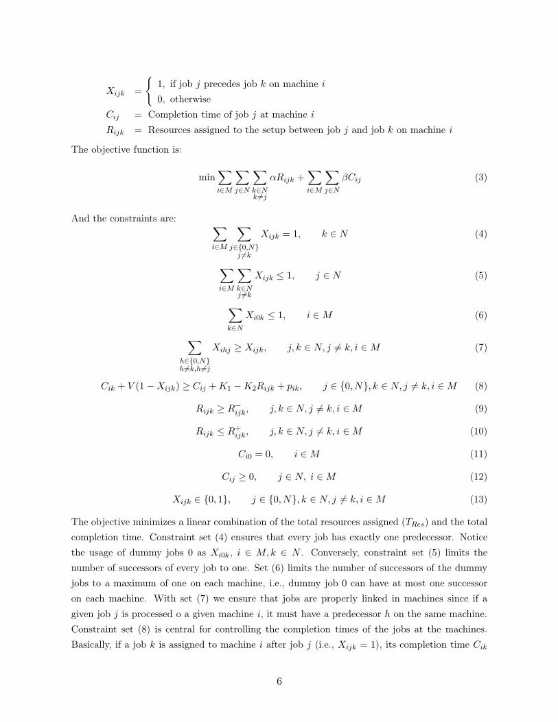
4.5 Application example

We present an example application of the DJASAav and DJASA∗av heuristics to a small four job,

2 machine problem. The processing times are given in Table 1 while the minimum and maximum

resources and setups are given in Table 2.

[Insert Tables 1 and 2 about here]

Now we apply the dynamic dispatching rule DJASAav. Let us work with α = 30 and β = 1,

10

i.e., each unit of resource is 30 times more expensive or important than each flowtime unit.

Additionally, we are going to assume that only an integer quantity of resources can be assigned.

Initially, all four jobs are unscheduled so ρ = 1, 2, 3, 4. Since we assume than the initial setups

are zero, the job with the shortest processing time on all machines is assigned. From Table 1 we

see that the lowest processing time corresponds to job 3 on machine 2 (p23 = 27). Therefore job

3 is scheduled first on machine 2. We remove job 3 from ρ.

Now we consider jobs all pending jobs ρ = 1, 2, 4 at machines 1 and 2:

1. Job 1, machine 1: C11 = C10 + S101 + p11 = 0+ 0+ 79 = 79. 79 units increase in objective.

2. Job 1, machine 2: Resources assigned:R

+

231+R

−

231

2 = 3 which correspond to S231 = 63.5.

C21 = C23 + S231 + p21 = 27 + 63.5 + 45 = 135.5. 30 · 3 + 135.5 = 225.5 units increase in

objective.

3. Job 2, machine 1: C12 = C10 + S102 + p12 = 0+ 0+ 51 = 51. 51 units increase in objective.


+

232+R

−

232


C22 = C23 + S232 + p22 = 27 + 59.5 + 78 = 164.5. 30 · 3 + 164.5 = 254.5 units increase in

objective.

5. Job 4, machine 1: C14 = C10 +S104 + p14 = 0+0+43 = 43. 43 units increase in objective.


+

234+R

−

234

2 = 3.5 → 4 which correspond to S234 =

36.3. C24 = C23 + S234 + p24 = 27 + 36.3 + 90 = 153.3. 30 · 4 + 153.3 = 273.3. 273.3 units

increase in objective.

The lowest increase in the objective comes after assigning job 4 to machine 2. Therefore, job 4 is

assigned first on machine 1. We remove job 4 from ρ.

Now we consider jobs all pending jobs ρ = 1, 2 at machines 1 and 2:


+

141+R

−

141


C11 = C14 +S141 +p11 = 43+54.5+79 = 176.5. 30 ·2+176.5 = 236.5. 236.5 units increase

in objective.


+

231+R

−

231


C21 = C23 + S231 + p21 = 27 + 63.5 + 45 = 135.5. 30 · 3 + 135.5 = 225.5. 225.5 units



+

142+R

−

142

2 = 3.5 → 4 which correspond to S142 = 36.

C12 = C14 + S142 + p12 = 43 + 36 + 51 = 130. 30 · 4 + 130 = 250. 250 units increase in

objective.


+

232+R

−

232


C22 = C23 +S232 +p22 = 27+59.5+78 = 164.5. 30 ·3+164.5 = 254.5. 254.5 units increase

in objective.

11

The lowest increase in the objective comes after assigning job 1 to machine 2. Job 1 is assigned

second on machine 2 and 3 units of resource are assigned to setup S231. We remove job 1 from ρ.

Now we consider the last pending job in ρ = 2 at machines 1 and 2:

1. Job 2, machine 1: Resources assigned:R+

142+R−

142


C12 = C14 + S142 + p12 = 43 + 36 + 51 = 130. 30 · 4 + 130 = 250. 250 units increase in

objective.


+

212+R

−

212


C22 = C21 + S212 + p22 = 135.5 + 34 + 78 = 247.5. 30 · 4 + 247.5 = 367.5. 367.5 units


In this last step, job 2 is assigned second on machine 2 and 4 units of resource are assigned to

setup S142. After removing job 2 from ρ we have that ρ = ∅ so the procedure is finished. In total

there are 4+3 = 7 resources assigned. The total completion time is 43+130+27+135.5 = 335.5

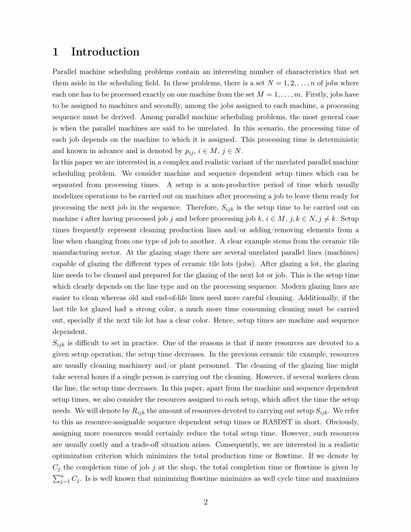
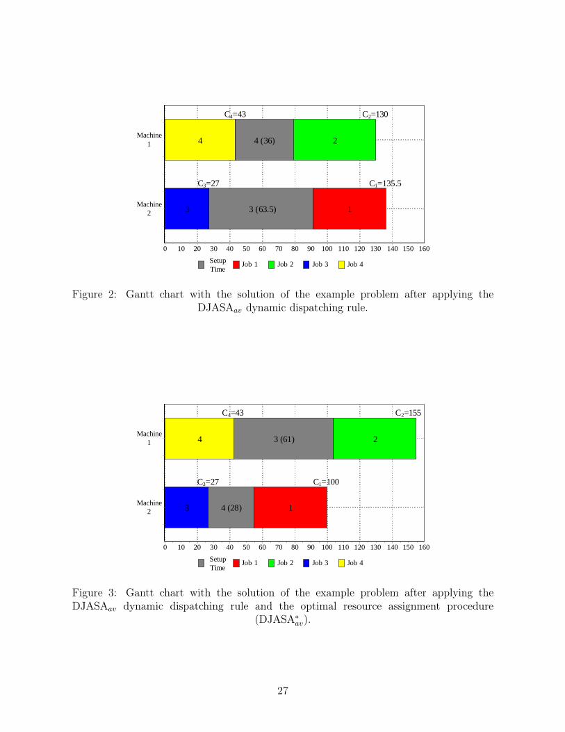
so the objective value is 30 · 7 + 335.5 = 545.5. A Gantt chart with this solution along with all

details is shown in Figure 2.


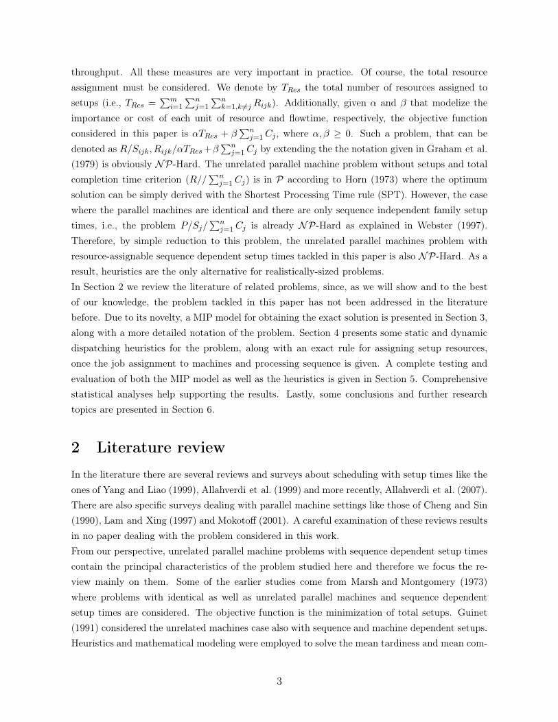
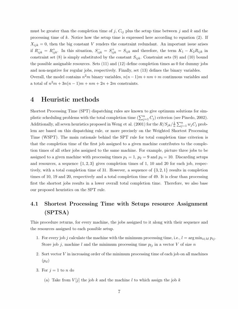
At this point, we apply the optimal resource assignment. We only have two setups in the example,

S142 = 36 with R142 = 4 and S231 = 63.5 with R231 = 3. There is one job after each setup on

both cases. Therefore:

1. Setup at machine 1 between jobs 4 and 2 (K2 = 25): K2 · 1 · 1 ≯ 30. Therefore R142 is

re-assigned to R−142 = 3. The objective value decreases by 5 units (α − K2).

2. Setup at machine 2 between jobs 3 and 1 (K2 = 35.5): K2 · 1 · 1 > 30. Therefore R231 is

re-assigned to R+231 = 4. The objective value decreases by 5.5 units (K2 − α).

As a result of the optimal resource assignment we have a new objective value of 545.5−5−5.5 =

535. The resulting Gantt chart is given in Figure 3.


5 Computational Evaluation

In this section our aim is to test the MIP model and the proposed heuristics for this novel

unrelated parallel machine RASDST problem. In order to do so, a comprehensive benchmark

has been defined. As has been shown in the previous example problem, apart from the number

of jobs n and the number of machines m, several sets of data have to be generated. These are

the processing times pij and the minimum and maximum resources and setups R−ijk

, R+ijk

, S−ijk

12

and S+ijk

, respectively. The MIP model is not expected to be usable for large instances, given

the number of variables and constraints needed. Therefore, two sets of instances are defined.

For the small instances, all the following combinations of n and m are tested: n = {6, 8, 10}

and m = {3, 4, 5}. For the large instances the combinations are n = {50, 75, 100} and m =

{10, 15, 20}. In all cases, the processing times are generated according to a uniform distribution

in the range [1, 99] as it is usual in the scheduling literature. For the minimum and maximum

resources we consider two combinations. In the first one the minimum and maximum resources

are uniformly distributed in the ranges [1, 3; 3, 5]. For the second case the uniform distributions

are [1, 5; 5, 10]. This means that R−ijk

is distributed as U [1, 3] and U [1, 5] and R+ijk

as U [3, 5] and

U [5, 10]. However, only two combinations are considered. For the setup times we also work with

two combinations U [1, 50; 50, 100] and U [50, 100; 100, 150]. These two cases modelize medium

and large setup times, respectively. Notice that there is a possibility of R−ijk being equal to R+

ijk.

We think this captures the reality in which some setups might not be resource-assignable. In

such cases the value of S−ijk is equal to S+

ijk.

As a conclusion, for the small instances we have three values for n, three for m, two combinations

of resources and two of setups. 10 instances are generated for each case so there are 360 small

instances. The same applies for the large instances so the total number of instances considered

is 720. In order to study both the MIP model and the heuristics, we set the weights for the

objective function as α = 50 and β = 1. The rationale behind this decision is that resources are

usually scarce and more expensive than each unit of flowtime.

5.1 MIP model performance study

We construct a model in LP format for each instance in the small set. The resulting 360 models

are solved with CPLEX 9.1 on a Pentium IV 3.2 GHz computer with 1 Gbyte of RAM memory.

We have refrained from developing an ad-hoc branch and bound method mainly due to the fact

that obtaining good lower bounds for the RASDST problem is deemed as complicated. The rea-

son is that lower bounds are weak in the presence of sequence dependent setup times. In simpler

scheduling environments no good lower bounds exist in the presence of sequence dependent setup

times since the amount of setups depends on the sequence. Furthermore, commercial solvers for

parallel machine problems with setups have also been used by Balakrishnan et al. (1999) and

Zhu and Heady (2000).

We solve all instances with two different time limits, 5 and 60 minutes. We think that allowing

more time is not realistic since scheduling problems need to be solved in a matter of minutes in

a production floor. As we will see, not all instances are solved within these time limits. Con-

sequently, for each run we record a categorical variable which we refer to as “type of solution”

with two possible values 0 and 1. Type 0 means that an optimum solution was found, in which

the objective value and the time needed for obtaining it are recorded. Type 1 means that the

time limit was reached and at the end a feasible integer solution was found. The gap is recorded

13

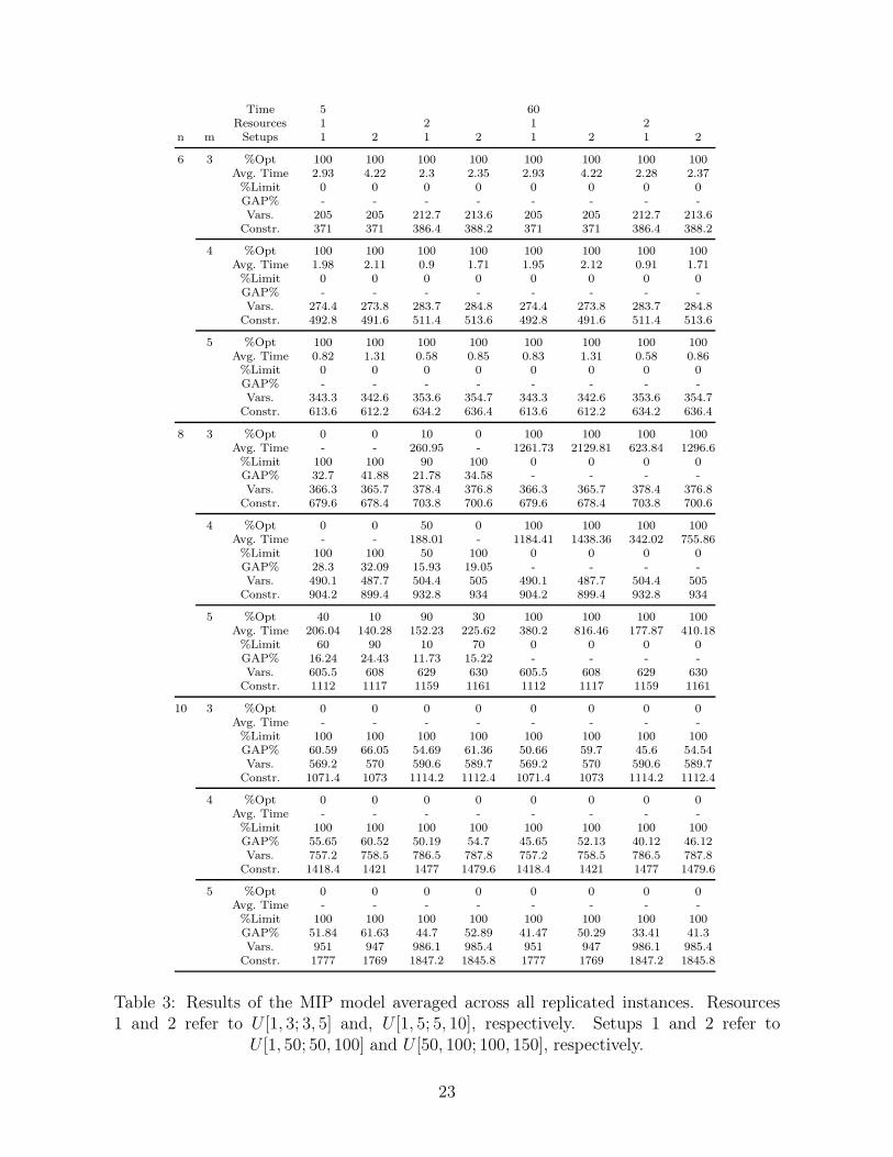
in such a case. The averaged results for all levels of n, m, Rijk and Sijk are given in Table 3.

Each cell gives the average of the 10 replicated instances. The percentage of instances for which

a type 0 solution was found (%Opt) and the average time needed for this optimum solution (Avg.

Time) are displayed. The percentage of instances with a type 1 solution (%Limit) is also shown

in the table along with the observed gap (GAP%). Finally, the average number of variables and

constraints is also given.

[Insert Table 3 about here]

Some direct conclusions can be drawn from Table 3. For example, all instances with n = 6 are

solved to optimality under both stopping time criteria. However, for n = 8, only a few optimum

solutions are obtained within 5 minutes CPU time. For 60 minutes CPU times, all n = 8 instances

are solved. For n = 10 no optimum solution could be found for any instance even with 60 minutes

CPU time. The effect of other factors is also easy to see. Increasing the number of machines m

results in instances that are easier to solve. At first, this observation might seem counterintuitive.

However, with fewer machines, more jobs are assigned to each machine and the importance of

the job sequence and sequence dependent setup times, as well as assignable resources, becomes

more visible. The largest CPU times among the solved instances are observed for n = 8 and

m = 3. The same applies to the largest gaps in unsolved instances (n = 10 and m = 3). The

effect of the resources is also interesting. From the Table it seems that having more resources

(i.e., U [1, 5; 5, 10]) results in instances that are easier to solve. On the other hand, larger setups

(U [50, 100; 100, 150]) result in harder instances. All these observations are important since they

allow us to characterize which elements from the novel unrelated parallel machines RASDST

problem affect performance. Lastly, we can see that the number of variables and constraints (as

reported by CPLEX after model reduction techniques) are largely affected by n and m, as the

other factors do not seem to contribute significantly.

Overall, the performance of the MIP model is good, specially when compared to results from

the literature. Balakrishnan et al. (1999) solved problems of up to n = 10 and m = 4 but on a sim-

pler setting with uniform parallel machines. Their MIP model contains significantly less variables

due to the triangular law of inequality assumption in the setup times, i.e., Balakrishnan et al.

(1999) assume that Sijk + Sikl ≥ Sijl. Obviously, in our RASDST problem this assumption is

unacceptable since the length of the setups might change greatly depending on the resources

assigned. Zhu and Heady (2000) work with an unrelated parallel machines case and use a similar

variable definition to the one employed in this paper. In this case, the largest size of problem

solved is n = 9 and m = 3 needing almost 5,400 seconds of CPU time in this latter case. Con-

sidering that in our model, apart from the job assignment and the job sequencing we have also

the assignable-resources, we conclude that the MIP model performance is good.

14

5.2 MIP model statistical analysis

All previous discussion is solely based on observed average values. It is important to carry out sta-

tistical testing in order to have a sound basis for the conclusions reached. We use a not so common

advanced statistical technique called Automatic Interaction Detection (AID). AID recursively bi-

sects experimental data according to one factor into mutually exclusive and exhaustive sets that

explain the variability in a given response variable in the best statistically significant way. AID

was originally proposed by Morgan and Sonquist (1963). Kass (1980) improved the initial AID

by including statistical significance testing in the partition process and by allowing multi-way

splits of the data. The improved version is called Chi-squared Automatic Interaction Detection

(CHAID). Biggs et al. (1991) developed an improved version known as Exhaustive CHAID. AID

techniques are a common tool in the fields of Education, Population Studies, Market Research,

Psychology, etc. CHAID was recently used by Ruiz et al. (2007) also for the analysis of a MIP

model.

We adopt the Exhaustive CHAID method for the analysis of the MIP model results. The pro-

cedure starts with all data contained in a root node. From this point, all controlled factors are

studied and the best multi-way split of the root node according to the levels of each factor is

calculated. A statistical significance test is carried out to rank the factors on the splitting capa-

bility. The procedure is applied recursively to all nodes until no more significant partitions can

be found. A decision tree is constructed from the splitting procedure. This tree allows a visual

and comprehensive study of the effect of the different factors on the studied response variable.

We use SPSS DecisionTree 3.0 software. The factors n, m, Resources and Setups are controlled.

We introduce all data of both stopping CPU time criteria, so the factor Time is also controlled.

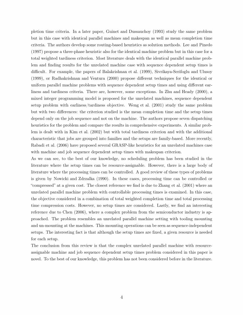
The response variable is the type of solution with two possible values (0 and 1). We set a high

confidence level for splitting of 99.9% and a Bonferroni adjustment for multi-way splits that com-

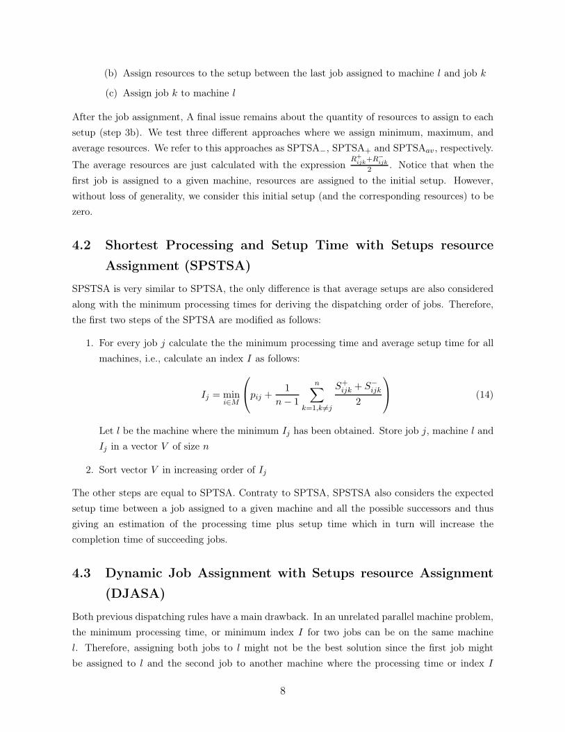
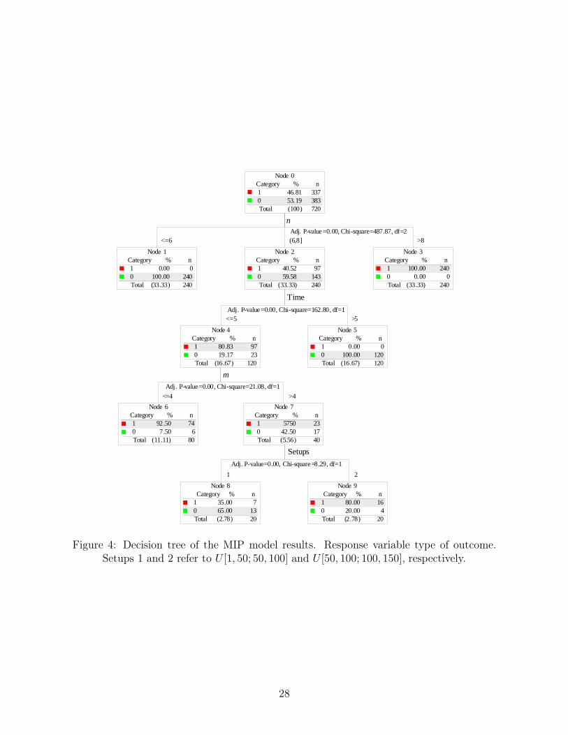
pensates the statistical bias in multi-way paired tests. The full decision tree is shown in Figure 4.


As with Table 3, the most important factor on determining the type of solution is n. As we can

see, the statistical test with which the root node has been split has a very large Chi-Square value

and an Adjusted P-Value of essentially 0. This means that the split is statistically significant at a

very high confidence level. This first level split statistically confirms that n is the most influential

factor on the type of solution. For instances of 8 jobs the situation is very interesting. First of

all, with 60 minutes CPU time, all instances are solved (second level split). For 5 minutes CPU

time, the tree has many other levels. The third split corresponds to the number of machines

m. According to this, instances with 4 or less machines are more difficult than instances with 5

machines. Lastly, for n = 8 Time=5 and m = 5, large setups result in harder instances.

It is also interesting to repeat the analysis but changing the response variable to the observed

gap percentage. In this case, the response variable is no longer categorical but rather continuous.

15

The resulting tree is very large and is not shown here for reasons of space. However, the following

observations can be made from the results:

• For n = 8 and Time=5 there is a large tree with one first split on m. In this case, the gap

percentage increases with decreasing values of m

• For n = 8, Time=5 and the different splits on m there are further splits. The overall

observation is that the gap percentage is larger for Resources = U [1, 5; 5, 10] and Setups =

U [50, 100; 100, 150]. This is consistent for all the multi-way splits according to the values

of m.

• For n = 10 and Time=5 the next split is based on Setups, not in m as in the previous case.

Again, larger setups result in larger gap percentages

• For n = 10, Time=5 and for the two values of setups, the trend for the resources is reversed,

i.e., more resources result in slighter lower gap percentages

• For n = 10 and Time=60 the next split is based in m, with larger gap percentages as m

decreases

• For n = 10, Time=60 and all the values for m, the following splits are either based on

Setups or on Resources. Again, larger setups result larger gap percentages.

• For n = 10, Time=60, values of m and all values of Setups, higher number of resources

results in lower gap percentages.

• The largest gap percentage under 60 minutes CPU time is observed for the following com-

bination of values: n = 10, m = 3, Setups=U [50, 100; 100, 150] and Resources=U [1, 3; 3, 5].

Here the gap percentage is almost 60%.

After this comprehensive analysis we know that for the MIP model the number of jobs and

machines clearly affect the difficulty. To be precise, a high n/m ratio results in the most difficult

problems. Large setups and low quantity of assignable resources also contribute to the difficulty.

5.3 Heuristic evaluation

We proceed now to test the performance of the proposed heurisics. Recall that there are three

main methods each one with three possible resource assignment variations: SPTSA−, SPTSA+,

SPTSAav , SPSTSA−, SPSTSA+, SPSTSAav , DJASA−, DJASA+ and DJASAav. Finally, we can

apply the optimal resource assignment procedure to SPTSA, SPSTSA and to the three DJASA

variants, this gives us five more methods: SPTSA∗, SPSTSA∗, DJASA∗−, DJASA∗

+ and DJASA∗av.

As a result, there are 14 different methods. All heuristics have been coded in Delphi 2006 and

have been tested on the same computer used for testing the MIP model.

16

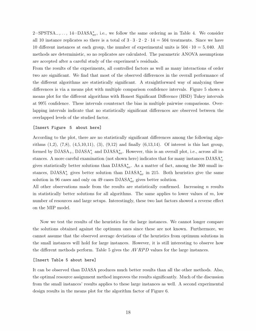
We test each method on the small instances, where we measure the average percentage increase

(AV RPD) over the optimum solution (or best solution found) given by the MIP model. For

the large instances we test the average percentage deviation over the best solution found by all

heuristics. The AV RPD is measured as follows:

AV RPD =1

R

R∑

r=1

Heusolr − Optsolr

Optsolr

100 (16)

where Heusolr is the heuristic solution obtained by any of the 14 methods on instance repli-

cate r. Optsolr is the MIP optimum or best solution known for that instance replicate and

for the small instances or the best solution known across all results for that instance replicate

for the large instances. All instances, as well as the best known solutions are available from

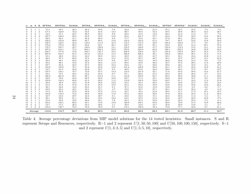
http://www.upv.es/gio/rruiz. Table 4 gives the AV RPD values for the small instances. The

results are shown for every possible combination of n, m, Setups and Resources. Recall that

there are 10 instances per each combination and therefore each cell contains the AV RPD across

10 values.


As expected, DJASA is the best method over SPSTSA and this later one is in turn better

than SPTSA. The AV RPD values drop strongly for DJASA in all situations. Among the three

resource assignment methods, (−, + and av) the best solutions are obtained by assigning the

maximum resources and the worst solutions by assigning the lowest resources. This is consistent

for the three heuristics. Obviously, increasing the value of α would favor assigning less resources.

As expected, the optimal resource assignment procedure improves the results always since the

procedure cannot deteriorate the solutions. What is more interesting is to actually quantify the

improvements. For example, comparing the best SPTSA method, SPTSA+ with SPTSA∗+ we see

a difference of 5.2%. This difference is 4.6% for SPSTSA and a mere 0.4% for DJASA. However,

the differences are much larger if we compare other initial resource assignments. The trend for n

and m is not clear. It seems that larger values of m result in higher AV RPD values. What seems

clear is the effect of the setups and resources. Higher number of resources and lower duration of

setups results in higher deviations.

Overall, the best result is given by algorithm DJASA∗+ with an average deviation from optimum

solutions of 11.1%. In reality, deviation from optimum solution can only be given for instances

with n ≤ 8. In this case, the AV RPD is 12.41%. While being relatively large, it is fairly small

considering that DJASA is a simple dispatching rule.

As with the case of the MIP model, the previous table contains observed averages alone. We

carry out a full experimental analysis using the ANOVA technique. In the experiment we control

n, m, R, S and Algorithm as factors. Algorithm is a factor with 14 levels where 1=SPTSA−,

17

http://www.upv.es/gio/rruiz

2=SPSTSA−,. . . , 14=DJASA∗av , i.e., we follow the same ordering as in Table 4. We consider

all 10 instance replicates so there is a total of 3 · 3 · 2 · 2 · 14 = 504 treatments. Since we have

10 different instances at each group, the number of experimental units is 504 · 10 = 5, 040. All

methods are deterministic, so no replicates are calculated. The parametric ANOVA assumptions

are accepted after a careful study of the experiment’s residuals.

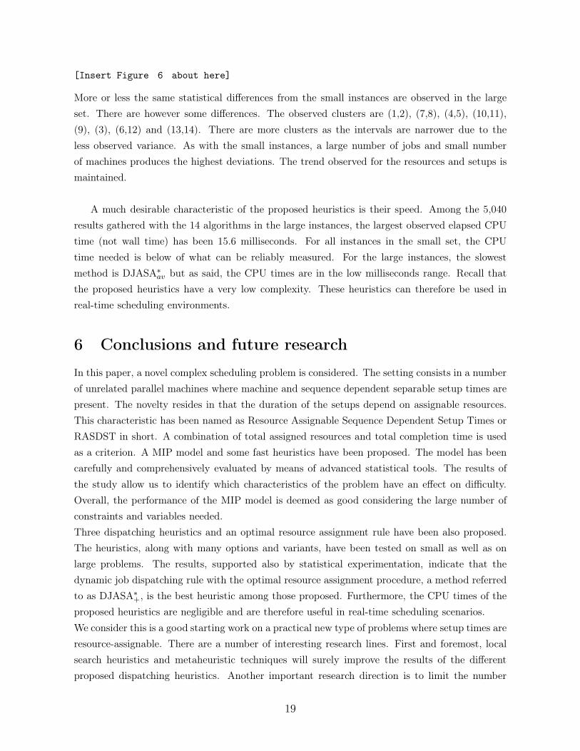
From the results of the experiments, all controlled factors as well as many interactions of order

two are significant. We find that most of the observed differences in the overall performance of

the different algorithms are statistically significant. A straightforward way of analyzing these

differences is via a means plot with multiple comparison confidence intervals. Figure 5 shows a

means plot for the different algorithms with Honest Significant Difference (HSD) Tukey intervals

at 99% confidence. These intervals counteract the bias in multiple pairwise comparisons. Over-

lapping intervals indicate that no statistically significant differences are observed between the

overlapped levels of the studied factor.


According to the plot, there are no statistically significant differences among the following algo-

rithms (1,2), (7,8), (4,5,10,11), (3), (9,12) and finally (6,13,14). Of interest is this last group,

formed by DJASA+, DJASA∗+ and DJASA∗

av. However, this is an overall plot, i.e., across all in-

stances. A more careful examination (not shown here) indicates that for many instances DJASA∗+

gives statistically better solutions than DJASA∗av . As a matter of fact, among the 360 small in-

stances, DJASA∗+ gives better solution than DJASA∗

av in 215. Both heuristics give the same

solution in 96 cases and only on 49 cases DJASA∗av gives better solution.

All other observations made from the results are statistically confirmed. Increasing n results

in statistically better solutions for all algorithms. The same applies to lower values of m, low

number of resources and large setups. Interestingly, these two last factors showed a reverse effect

on the MIP model.

Now we test the results of the heuristics for the large instances. We cannot longer compare

the solutions obtained against the optimum ones since these are not known. Furthermore, we

cannot assume that the observed average deviations of the heuristics from optimum solutions in

the small instances will hold for large instances. However, it is still interesting to observe how

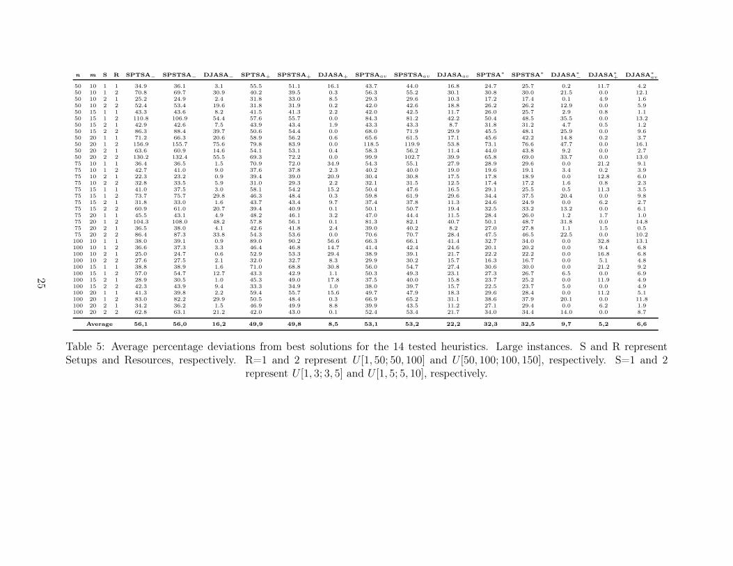
the different methods perform. Table 5 gives the AV RPD values for the large instances.


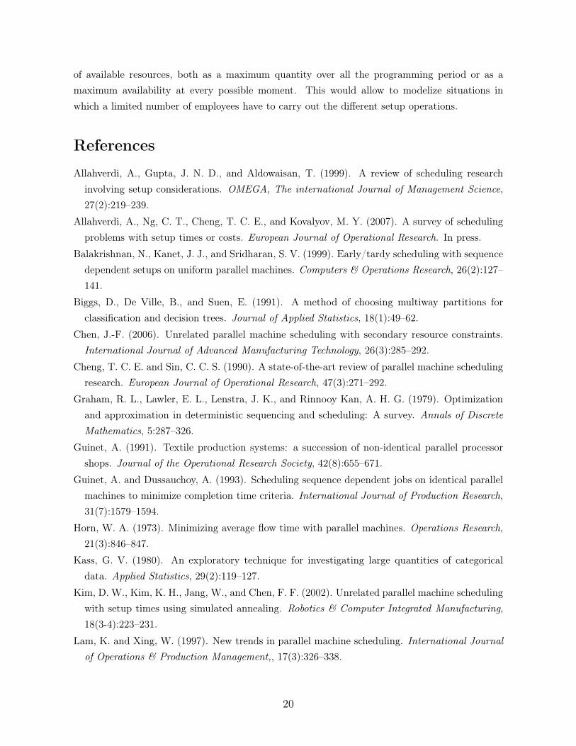
It can be observed than DJASA produces much better results than all the other methods. Also,

the optimal resource assignment method improves the results significantly. Much of the discussion

from the small instances’ results applies to these large instances as well. A second experimental

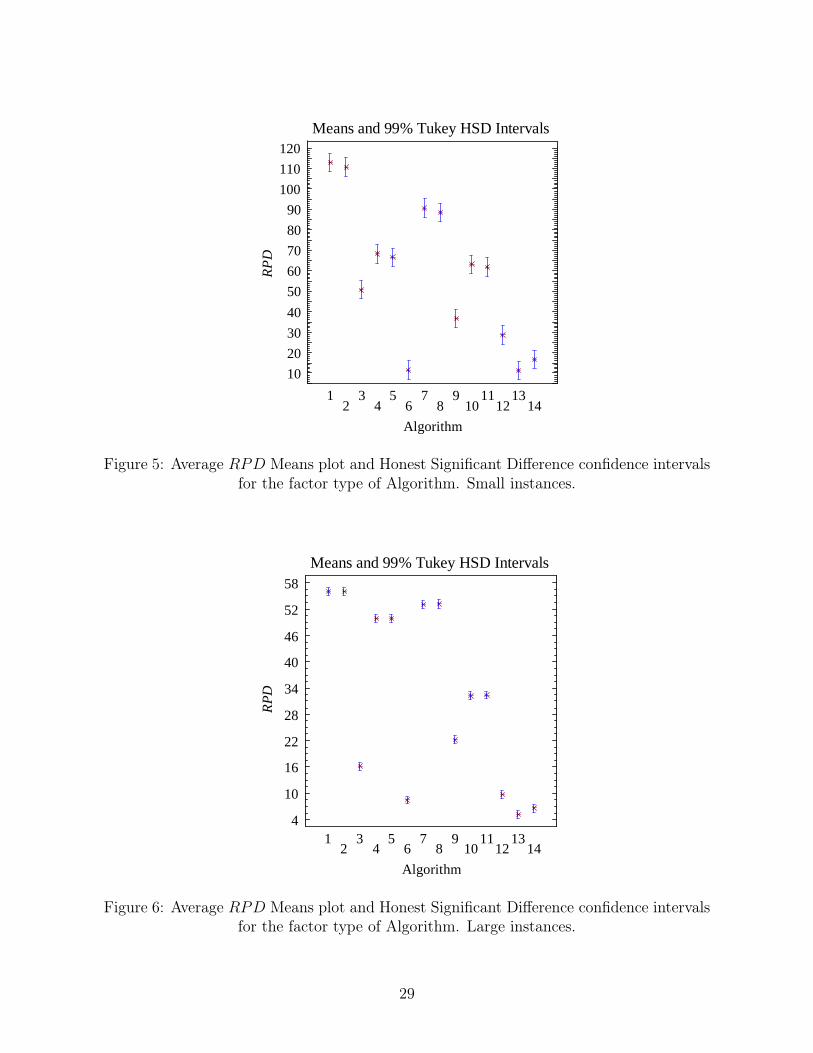
design results in the means plot for the algorithm factor of Figure 6.

18


More or less the same statistical differences from the small instances are observed in the large

set. There are however some differences. The observed clusters are (1,2), (7,8), (4,5), (10,11),

(9), (3), (6,12) and (13,14). There are more clusters as the intervals are narrower due to the

less observed variance. As with the small instances, a large number of jobs and small number

of machines produces the highest deviations. The trend observed for the resources and setups is

maintained.

A much desirable characteristic of the proposed heuristics is their speed. Among the 5,040

results gathered with the 14 algorithms in the large instances, the largest observed elapsed CPU

time (not wall time) has been 15.6 milliseconds. For all instances in the small set, the CPU

time needed is below of what can be reliably measured. For the large instances, the slowest

method is DJASA∗av but as said, the CPU times are in the low milliseconds range. Recall that

the proposed heuristics have a very low complexity. These heuristics can therefore be used in

real-time scheduling environments.

6 Conclusions and future research

In this paper, a novel complex scheduling problem is considered. The setting consists in a number

of unrelated parallel machines where machine and sequence dependent separable setup times are

present. The novelty resides in that the duration of the setups depend on assignable resources.

This characteristic has been named as Resource Assignable Sequence Dependent Setup Times or

RASDST in short. A combination of total assigned resources and total completion time is used

as a criterion. A MIP model and some fast heuristics have been proposed. The model has been

carefully and comprehensively evaluated by means of advanced statistical tools. The results of

the study allow us to identify which characteristics of the problem have an effect on difficulty.

Overall, the performance of the MIP model is deemed as good considering the large number of

constraints and variables needed.

Three dispatching heuristics and an optimal resource assignment rule have been also proposed.

The heuristics, along with many options and variants, have been tested on small as well as on

large problems. The results, supported also by statistical experimentation, indicate that the

dynamic job dispatching rule with the optimal resource assignment procedure, a method referred

to as DJASA∗+, is the best heuristic among those proposed. Furthermore, the CPU times of the

proposed heuristics are negligible and are therefore useful in real-time scheduling scenarios.

We consider this is a good starting work on a practical new type of problems where setup times are

resource-assignable. There are a number of interesting research lines. First and foremost, local

search heuristics and metaheuristic techniques will surely improve the results of the different

proposed dispatching heuristics. Another important research direction is to limit the number

19

of available resources, both as a maximum quantity over all the programming period or as a

maximum availability at every possible moment. This would allow to modelize situations in

which a limited number of employees have to carry out the different setup operations.

References

Allahverdi, A., Gupta, J. N. D., and Aldowaisan, T. (1999). A review of scheduling research

involving setup considerations. OMEGA, The international Journal of Management Science,

27(2):219–239.

Allahverdi, A., Ng, C. T., Cheng, T. C. E., and Kovalyov, M. Y. (2007). A survey of scheduling

problems with setup times or costs. European Journal of Operational Research. In press.

Balakrishnan, N., Kanet, J. J., and Sridharan, S. V. (1999). Early/tardy scheduling with sequence

dependent setups on uniform parallel machines. Computers & Operations Research, 26(2):127–

141.

Biggs, D., De Ville, B., and Suen, E. (1991). A method of choosing multiway partitions for

classification and decision trees. Journal of Applied Statistics, 18(1):49–62.

Chen, J.-F. (2006). Unrelated parallel machine scheduling with secondary resource constraints.

International Journal of Advanced Manufacturing Technology, 26(3):285–292.

Cheng, T. C. E. and Sin, C. C. S. (1990). A state-of-the-art review of parallel machine scheduling

research. European Journal of Operational Research, 47(3):271–292.

Graham, R. L., Lawler, E. L., Lenstra, J. K., and Rinnooy Kan, A. H. G. (1979). Optimization

and approximation in deterministic sequencing and scheduling: A survey. Annals of Discrete

Mathematics, 5:287–326.

Guinet, A. (1991). Textile production systems: a succession of non-identical parallel processor

shops. Journal of the Operational Research Society, 42(8):655–671.

Guinet, A. and Dussauchoy, A. (1993). Scheduling sequence dependent jobs on identical parallel

machines to minimize completion time criteria. International Journal of Production Research,

31(7):1579–1594.

Horn, W. A. (1973). Minimizing average flow time with parallel machines. Operations Research,

21(3):846–847.

Kass, G. V. (1980). An exploratory technique for investigating large quantities of categorical

data. Applied Statistics, 29(2):119–127.

Kim, D. W., Kim, K. H., Jang, W., and Chen, F. F. (2002). Unrelated parallel machine scheduling

with setup times using simulated annealing. Robotics & Computer Integrated Manufacturing,

18(3-4):223–231.

Lam, K. and Xing, W. (1997). New trends in parallel machine scheduling. International Journal

of Operations & Production Management,, 17(3):326–338.

20

Lee, Y. H. and Pinedo, M. (1997). Scheduling jobs on parallel machines with sequence dependent

setup times. European Journal of Operational Research, 100(3):464–474.

Marsh, J. D. and Montgomery, D. C. (1973). Optimal procedures for scheduling jobs with

sequence-dependent changeover times on parallel processors. AIIE Technical Papers, pages

279–286.

Mokotoff, E. (2001). Parallel machine scheduling problems: a survey. Asia-Pacific Journal of

Operational Research, 18(2):193–242.

Morgan, J. A. and Sonquist, J. N. (1963). Problems in the analysis of survey data and a proposal.

Journal of the American Statistical Association, 58:415–434.

Nowicki, E. and Zdrzalka, S. (1990). A survey of results for sequencing problems with controllable

processing times. Discrete Applied Mathematics, 26(2-3):271–287.

Pinedo, M. (2002). Scheduling: Theory, Algorithms, and Systems. Prentice Hall, Upper Saddle,

N.J, second edition.

Rabadi, G., Moraga, R. J., and Al-Salem, A. (2006). Heuristics for the unrelated parallel machine

scheduling problem with setup times. Journal of Intelligent Manufacturing, 17(1):85–97.

Radhakrishnan, S. and Ventura, J. A. (2000). Simulated annealing for parallel machine scheduling

with earliness-tardiness penalties and sequence-dependent set-up times. International Journal

of Production Research, 38(10):2233–2252.

Ruiz, R., Sivrikaya Şerifoğlu, F., and Urlings, T. (2007). Modeling realistic hybrid flexible flow-

shop scheduling problems. Computers & Operations Research. In press.

Sivrikaya-Serifoglu, F. and Ulusoy, G. (1999). Parallel machine scheduling with earliness and

tardiness penalties. Computers & Operations Research, 26(8):773–787.

Webster, S. T. (1997). The complexity of scheduling job families about a common due date.

Operations Research Letters, 20(2):65–74.

Weng, M. X., Lu, J., and Ren, H. (2001). Unrelated parallel machines scheduling with setup con-

sideration and a total weighted completion time objective. International Journal of Production

Economics, 70(3):215–226.

Yang, W.-H. and Liao, C.-J. (1999). Survey of scheduling research involving setup times. Inter-

national Journal of Systems Science, 30(2):143–155.

Zhang, F., Tang, G. C., and Chen, Z. L. (2001). A 3/2-approximation algorithm for parallel

machine scheduling with controllable processing times. Operations Research Letters, 29(1):41–

47.

Zhu, Z. and Heady, R. (2000). Minimizing the sum of earliness/tardiness in multi-machine

scheduling: a mixed integer programming approach. Computers & Industrial Engineering,

38(2):297–305.

21

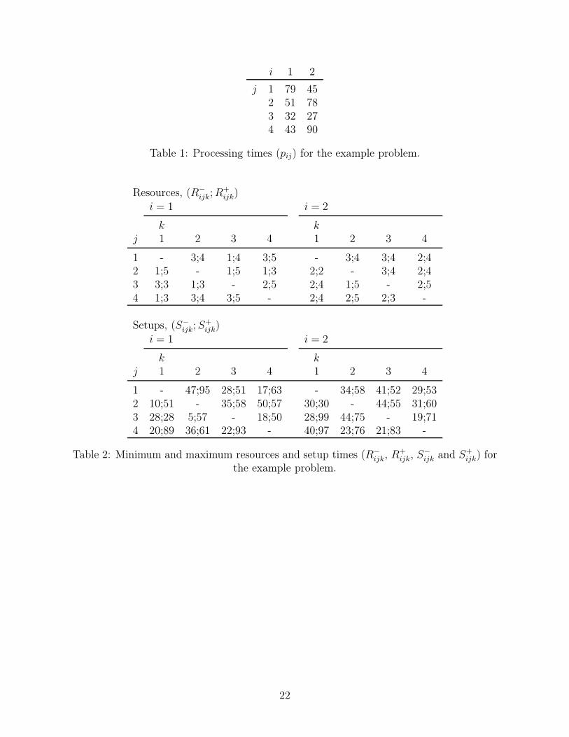
i 1 2

j 1 79 452 51 783 32 274 43 90

Table 1: Processing times (pij) for the example problem.

Resources, (R−ijk; R

+ijk)

i = 1 i = 2

k k

j 1 2 3 4 1 2 3 4

1 - 3;4 1;4 3;5 - 3;4 3;4 2;42 1;5 - 1;5 1;3 2;2 - 3;4 2;43 3;3 1;3 - 2;5 2;4 1;5 - 2;54 1;3 3;4 3;5 - 2;4 2;5 2;3 -

Setups, (S−ijk; S

+ijk)

i = 1 i = 2

k k

j 1 2 3 4 1 2 3 4

1 - 47;95 28;51 17;63 - 34;58 41;52 29;532 10;51 - 35;58 50;57 30;30 - 44;55 31;603 28;28 5;57 - 18;50 28;99 44;75 - 19;714 20;89 36;61 22;93 - 40;97 23;76 21;83 -

Table 2: Minimum and maximum resources and setup times (R−ijk, R+

ijk, S−ijk and S+

ijk) forthe example problem.

22

Time 5 60Resources 1 2 1 2

n m Setups 1 2 1 2 1 2 1 2

6 3 %Opt 100 100 100 100 100 100 100 100Avg. Time 2.93 4.22 2.3 2.35 2.93 4.22 2.28 2.37%Limit 0 0 0 0 0 0 0 0GAP% - - - - - - - -Vars. 205 205 212.7 213.6 205 205 212.7 213.6

Constr. 371 371 386.4 388.2 371 371 386.4 388.2

4 %Opt 100 100 100 100 100 100 100 100Avg. Time 1.98 2.11 0.9 1.71 1.95 2.12 0.91 1.71%Limit 0 0 0 0 0 0 0 0GAP% - - - - - - - -Vars. 274.4 273.8 283.7 284.8 274.4 273.8 283.7 284.8

Constr. 492.8 491.6 511.4 513.6 492.8 491.6 511.4 513.6

5 %Opt 100 100 100 100 100 100 100 100Avg. Time 0.82 1.31 0.58 0.85 0.83 1.31 0.58 0.86%Limit 0 0 0 0 0 0 0 0GAP% - - - - - - - -Vars. 343.3 342.6 353.6 354.7 343.3 342.6 353.6 354.7

Constr. 613.6 612.2 634.2 636.4 613.6 612.2 634.2 636.4

8 3 %Opt 0 0 10 0 100 100 100 100Avg. Time - - 260.95 - 1261.73 2129.81 623.84 1296.6%Limit 100 100 90 100 0 0 0 0GAP% 32.7 41.88 21.78 34.58 - - - -Vars. 366.3 365.7 378.4 376.8 366.3 365.7 378.4 376.8

Constr. 679.6 678.4 703.8 700.6 679.6 678.4 703.8 700.6

4 %Opt 0 0 50 0 100 100 100 100Avg. Time - - 188.01 - 1184.41 1438.36 342.02 755.86%Limit 100 100 50 100 0 0 0 0GAP% 28.3 32.09 15.93 19.05 - - - -Vars. 490.1 487.7 504.4 505 490.1 487.7 504.4 505

Constr. 904.2 899.4 932.8 934 904.2 899.4 932.8 934

5 %Opt 40 10 90 30 100 100 100 100Avg. Time 206.04 140.28 152.23 225.62 380.2 816.46 177.87 410.18%Limit 60 90 10 70 0 0 0 0GAP% 16.24 24.43 11.73 15.22 - - - -Vars. 605.5 608 629 630 605.5 608 629 630

Constr. 1112 1117 1159 1161 1112 1117 1159 1161

10 3 %Opt 0 0 0 0 0 0 0 0Avg. Time - - - - - - - -%Limit 100 100 100 100 100 100 100 100GAP% 60.59 66.05 54.69 61.36 50.66 59.7 45.6 54.54Vars. 569.2 570 590.6 589.7 569.2 570 590.6 589.7

Constr. 1071.4 1073 1114.2 1112.4 1071.4 1073 1114.2 1112.4

4 %Opt 0 0 0 0 0 0 0 0Avg. Time - - - - - - - -%Limit 100 100 100 100 100 100 100 100GAP% 55.65 60.52 50.19 54.7 45.65 52.13 40.12 46.12Vars. 757.2 758.5 786.5 787.8 757.2 758.5 786.5 787.8

Constr. 1418.4 1421 1477 1479.6 1418.4 1421 1477 1479.6

5 %Opt 0 0 0 0 0 0 0 0Avg. Time - - - - - - - -%Limit 100 100 100 100 100 100 100 100GAP% 51.84 61.63 44.7 52.89 41.47 50.29 33.41 41.3Vars. 951 947 986.1 985.4 951 947 986.1 985.4

Constr. 1777 1769 1847.2 1845.8 1777 1769 1847.2 1845.8

Table 3: Results of the MIP model averaged across all replicated instances. Resources1 and 2 refer to U [1, 3; 3, 5] and, U [1, 5; 5, 10], respectively. Setups 1 and 2 refer to

U [1, 50; 50, 100] and U [50, 100; 100, 150], respectively.

23

n m S R SPTSA−

SPSTSA−

DJASA−

SPTSA+ SPSTSA+ DJASA+ SPTSAav SPSTSAav DJASAav SPTSA∗ SPSTSA∗ DJASA∗

−DJASA∗

+ DJASA∗

av

6 3 1 1 57.4 58.5 36.5 46.2 50.6 7.6 52.2 54.6 21.3 37.1 42.7 19.3 7.2 7.2

6 3 1 2 117.1 124.8 72.2 55.5 61.9 12.4 88.7 95.0 52.4 50.5 56.9 38.3 12.4 26.7

6 3 2 1 44.5 47.1 20.7 29.3 36.2 6.6 36.9 41.0 14.3 26.4 31.2 11.2 5.7 7.2

6 3 2 2 127.7 128.9 90.9 65.9 76.6 15.6 95.6 101.7 57.7 63.0 73.8 43.5 15.6 20.5

6 4 1 1 82.5 84.4 31.1 65.4 66.4 9.8 71.7 75.0 23.1 57.9 60.1 23.3 9.8 16.8

6 4 1 2 169.5 155.8 88.8 82.7 89.3 15.8 124.3 123.2 61.4 78.7 80.7 54.9 15.8 20.2

6 4 2 1 128.7 124.5 32.4 110.0 111.0 10.3 116.7 113.3 23.9 104.3 102.0 17.7 9.8 15.7

6 4 2 2 172.3 175.0 80.7 94.0 82.1 20.1 132.7 129.1 60.1 93.2 82.0 41.4 20.1 37.0

6 5 1 1 176.7 165.1 30.7 136.6 120.6 12.1 152.5 140.6 21.7 125.0 112.5 13.5 12.1 13.5

6 5 1 2 337.4 416.1 77.4 204.1 232.5 23.9 270.6 324.9 60.2 199.1 232.5 44.9 23.9 34.0

6 5 2 1 224.7 177.0 37.6 194.7 145.7 16.5 209.3 158.3 25.7 185.6 135.0 26.7 16.3 17.0

6 5 2 2 287.0 244.7 67.5 161.8 155.2 13.4 226.9 206.4 48.1 159.2 150.8 36.7 13.4 17.5

8 3 1 1 53.1 48.9 25.4 42.3 38.9 13.1 46.9 43.5 21.7 33.1 30.1 16.4 10.8 11.5

8 3 1 2 96.5 97.3 66.0 37.5 34.4 15.1 67.8 65.7 46.7 35.1 33.7 33.7 15.1 21.8

8 3 2 1 39.3 38.1 22.3 32.5 27.9 9.8 36.7 33.2 16.3 26.3 24.6 10.4 8.8 7.8

8 3 2 2 90.3 88.1 53.2 47.4 38.4 11.8 69.0 63.6 40.3 45.7 37.4 28.5 11.8 20.9

8 4 1 1 60.7 63.4 30.3 47.5 49.0 10.4 53.4 54.1 22.6 39.2 42.1 16.5 9.4 9.9

8 4 1 2 134.9 135.0 78.1 65.2 65.6 15.6 101.4 100.8 56.8 63.1 63.7 45.2 15.6 21.5

8 4 2 1 54.7 61.9 29.0 43.8 50.7 8.5 48.8 55.8 22.9 38.0 46.5 15.7 8.5 12.7

8 4 2 2 143.7 134.1 76.7 74.8 67.7 14.4 110.5 101.9 53.1 71.8 65.4 40.9 14.4 21.7

8 5 1 1 84.4 75.5 39.4 52.2 50.0 9.7 67.1 60.2 27.4 50.3 46.5 26.3 9.7 13.5

8 5 1 2 186.4 201.0 89.1 96.1 101.0 11.1 144.2 150.0 62.1 90.3 99.2 46.8 11.1 22.0

8 5 2 1 93.9 76.8 30.0 66.5 63.9 10.8 80.7 71.4 24.1 62.9 58.6 19.7 9.8 13.0

8 5 2 2 159.9 144.4 80.6 61.4 62.0 11.2 112.9 104.3 52.6 60.5 61.1 42.3 11.2 21.8

10 3 1 1 36.8 36.0 19.3 31.8 30.5 12.0 34.5 33.4 20.5 19.6 18.9 12.7 9.9 10.5

10 3 1 2 91.2 91.0 57.8 41.3 35.7 13.0 65.3 64.2 44.8 34.6 30.6 34.8 13.0 20.1

10 3 2 1 28.1 24.6 12.0 24.5 21.7 8.1 27.1 21.6 13.2 16.8 14.7 6.9 6.6 5.7

10 3 2 2 62.6 68.3 42.5 32.1 37.1 4.7 47.6 52.7 27.1 29.1 34.4 20.3 4.6 11.0

10 4 1 1 51.2 50.6 27.6 34.9 37.0 11.2 43.7 45.3 21.6 29.5 31.1 17.3 10.1 10.7

10 4 1 2 124.3 118.3 75.5 50.8 49.0 11.8 87.2 83.6 56.6 47.9 45.0 50.2 11.4 22.9

10 4 2 1 44.7 44.6 20.7 42.3 38.7 6.1 43.8 42.3 15.1 32.3 30.5 11.4 5.4 6.1

10 4 2 2 90.1 90.5 61.1 38.6 43.5 10.8 64.5 67.0 41.9 35.6 40.7 32.9 10.8 17.5

10 5 1 1 55.8 59.8 33.0 36.6 35.1 7.8 45.2 47.2 23.8 30.5 30.2 23.4 7.2 11.1

10 5 1 2 163.1 142.1 86.0 93.1 74.0 12.9 126.9 109.1 64.0 89.8 72.0 51.0 12.9 28.2

10 5 2 1 54.7 51.5 26.3 43.5 36.6 4.1 48.9 44.9 16.7 35.8 32.9 13.6 4.1 5.7

10 5 2 2 143.3 140.7 76.6 76.3 78.0 6.7 110.1 109.9 53.4 73.8 77.1 43.6 6.7 21.1

Average 113.0 110.7 50.7 68.3 66.5 11.5 90.6 88.6 36.5 63.1 61.9 28.7 11.1 16.7

Table 4: Average percentage deviations from MIP model solutions for the 14 tested heuristics. Small instances. S and Rrepresent Setups and Resources, respectively. R=1 and 2 represent U [1, 50; 50, 100] and U [50, 100; 100, 150], respectively. S=1

and 2 represent U [1, 3; 3, 5] and U [1, 5; 5, 10], respectively.

24

n m S R SPTSA−

SPSTSA−

DJASA−

SPTSA+ SPSTSA+ DJASA+ SPTSAav SPSTSAav DJASAav SPTSA∗ SPSTSA∗ DJASA∗

−DJASA∗

+ DJASA∗

av

50 10 1 1 34.9 36.1 3.1 55.5 51.1 16.1 43.7 44.0 16.8 24.7 25.7 0.2 11.7 4.2

50 10 1 2 70.8 69.7 30.9 40.2 39.5 0.3 56.3 55.2 30.1 30.8 30.0 21.5 0.0 12.1

50 10 2 1 25.2 24.9 2.4 31.8 33.0 8.5 29.3 29.6 10.3 17.2 17.4 0.1 4.9 1.6

50 10 2 2 52.4 53.4 19.6 31.8 31.9 0.2 42.0 42.6 18.8 26.2 26.2 12.9 0.0 5.9

50 15 1 1 43.3 43.6 8.2 41.5 41.3 2.2 42.0 42.5 11.7 26.0 25.7 2.9 0.8 1.1

50 15 1 2 110.8 106.9 54.4 57.6 55.7 0.0 84.3 81.2 42.2 50.4 48.5 35.5 0.0 13.2

50 15 2 1 42.9 42.6 7.5 43.9 43.4 1.9 43.3 43.3 8.7 31.8 31.2 4.7 0.5 1.2

50 15 2 2 86.3 88.4 39.7 50.6 54.4 0.0 68.0 71.9 29.9 45.5 48.1 25.9 0.0 9.6

50 20 1 1 71.2 66.3 20.6 58.9 56.2 0.6 65.6 61.5 17.1 45.6 42.2 14.8 0.2 3.7

50 20 1 2 156.9 155.7 75.6 79.8 83.9 0.0 118.5 119.9 53.8 73.1 76.6 47.7 0.0 16.1

50 20 2 1 63.6 60.9 14.6 54.1 53.1 0.4 58.3 56.2 11.4 44.0 43.8 9.2 0.0 2.7

50 20 2 2 130.2 132.4 55.5 69.3 72.2 0.0 99.9 102.7 39.9 65.8 69.0 33.7 0.0 13.0

75 10 1 1 36.4 36.5 1.5 70.9 72.0 34.9 54.3 55.1 27.9 28.9 29.6 0.0 21.2 9.1

75 10 1 2 42.7 41.0 9.0 37.6 37.8 2.3 40.2 40.0 19.0 19.6 19.1 3.4 0.2 3.9

75 10 2 1 22.3 23.2 0.9 39.4 39.0 20.9 30.4 30.8 17.5 17.8 18.9 0.0 12.8 6.0

75 10 2 2 32.8 33.5 5.9 31.0 29.3 2.2 32.1 31.5 12.5 17.4 17.2 1.6 0.8 2.3

75 15 1 1 41.0 37.5 3.0 58.1 54.2 15.2 50.4 47.6 16.5 29.1 25.5 0.5 11.3 3.5

75 15 1 2 73.7 75.7 29.8 46.3 48.4 0.3 59.8 61.9 29.6 34.4 37.5 20.4 0.0 9.8

75 15 2 1 31.8 33.0 1.6 43.7 43.4 9.7 37.4 37.8 11.3 24.6 24.9 0.0 6.2 2.7

75 15 2 2 60.9 61.0 20.7 39.4 40.9 0.1 50.1 50.7 19.4 32.5 33.2 13.2 0.0 6.1

75 20 1 1 45.5 43.1 4.9 48.2 46.1 3.2 47.0 44.4 11.5 28.4 26.0 1.2 1.7 1.0

75 20 1 2 104.3 108.0 48.2 57.8 56.1 0.1 81.3 82.1 40.7 50.1 48.7 31.8 0.0 14.8

75 20 2 1 36.5 38.0 4.1 42.6 41.8 2.4 39.0 40.2 8.2 27.0 27.8 1.1 1.5 0.5

75 20 2 2 86.4 87.3 33.8 54.3 53.6 0.0 70.6 70.7 28.4 47.5 46.5 22.5 0.0 10.2

100 10 1 1 38.0 39.1 0.9 89.0 90.2 56.6 66.3 66.1 41.4 32.7 34.0 0.0 32.8 13.1

100 10 1 2 36.6 37.3 3.3 46.4 46.8 14.7 41.4 42.4 24.6 20.1 20.2 0.0 9.4 6.8

100 10 2 1 25.0 24.7 0.6 52.9 53.3 29.4 38.9 39.1 21.7 22.2 22.2 0.0 16.8 6.8

100 10 2 2 27.6 27.5 2.1 32.0 32.7 8.3 29.9 30.2 15.7 16.3 16.7 0.0 5.1 4.8

100 15 1 1 38.8 38.9 1.6 71.0 68.8 30.8 56.0 54.7 27.4 30.6 30.0 0.0 21.2 9.2

100 15 1 2 57.0 54.7 12.7 43.3 42.9 1.1 50.3 49.3 23.1 27.3 26.7 6.5 0.0 6.9

100 15 2 1 28.9 30.5 1.0 45.3 49.0 17.8 37.5 40.0 15.8 23.7 25.2 0.0 11.9 4.9

100 15 2 2 42.3 43.9 9.4 33.3 34.9 1.0 38.0 39.7 15.7 22.5 23.7 5.0 0.0 4.9

100 20 1 1 41.3 39.8 2.2 59.4 55.7 15.6 49.7 47.9 18.3 29.6 28.4 0.0 11.2 5.1

100 20 1 2 83.0 82.2 29.9 50.5 48.4 0.3 66.9 65.2 31.1 38.6 37.9 20.1 0.0 11.8

100 20 2 1 34.2 36.2 1.5 46.9 49.9 8.8 39.9 43.5 11.2 27.1 29.4 0.0 6.2 1.9

100 20 2 2 62.8 63.1 21.2 42.0 43.0 0.1 52.4 53.4 21.7 34.0 34.4 14.0 0.0 8.7

Average 56,1 56,0 16,2 49,9 49,8 8,5 53,1 53,2 22,2 32,3 32,5 9,7 5,2 6,6

Table 5: Average percentage deviations from best solutions for the 14 tested heuristics. Large instances. S and R representSetups and Resources, respectively. R=1 and 2 represent U [1, 50; 50, 100] and U [50, 100; 100, 150], respectively. S=1 and 2

represent U [1, 3; 3, 5] and U [1, 5; 5, 10], respectively.

25

Rijk+RijkRijk

-

Sijk-

Sijk+

Sijk

Rijk ,- Sijk

+

Rijk , Sijk

Rijk ,+ Sijk-

Figure 1: Relation between setup time Sijk and number of assigned resources Rijk.

26

4 (36)

3 (63.5) 1

2

3

4

Setup Time

Job 1 Job 2 Job 3 Job 4

1601501401301201101009080706050403020100

Machine 1

Machine 2

C3=27 C1=135.5

C4=43 C2=130

Figure 2: Gantt chart with the solution of the example problem after applying theDJASAav dynamic dispatching rule.

Setup Time

Job 1 Job 2 Job 3 Job 4

1601501401301201101009080706050403020100

Machine 1

Machine 2

3 (61)

4 (28) 1

24

C3=27 C1=100

C4=43 C2=155

3

Figure 3: Gantt chart with the solution of the example problem after applying theDJASAav dynamic dispatching rule and the optimal resource assignment procedure

(DJASA∗av).

27

Category % n1 46.81 3370 53.19 383Total (100) 720

Node 0

Category % n1 100.00 2400 0.00 0Total (33.33) 240

Node 3Category % n1 40.52 970 59.58 143Total (33.33) 240

Node 2

Category % n1 0.00 00 100.00 120Total (16.67) 120

Node 5Category % n1 80.83 970 19.17 23Total (16.67) 120

Node 4

Category % n1 5750 230 42.50 17Total (5.56) 40

Node 7

Category % n1 80.00 160 20.00 4Total (2.78) 20

Node 9Category % n

1 35.00 70 65.00 13Total (2.78) 20

Node 8

Category % n1 92.50 740 7.50 6Total (11.11) 80

Node 6

Category % n1 0.00 00 100.00 240Total (33.33) 240

Node 1

nAdj. P-value=0.00, Chi-square=487.87, df=2

>8(6,8]

Time

Adj. P-value=0.00, Chi-square=162.80, df=1>5<=5

mAdj. P-value=0.00, Chi-square=21.08, df=1

>4

Setups

Adj. P-value=0.00, Chi-square=8.29, df=1

21

<=4

<=6

Figure 4: Decision tree of the MIP model results. Response variable type of outcome.Setups 1 and 2 refer to U [1, 50; 50, 100] and U [50, 100; 100, 150], respectively.

28

Means and 99% Tukey HSD Intervals

Algorithm

RP

D

12

34

56

78

910

1112

1314

10

20

30

40

50

60

70

80

90

100

110

120

Figure 5: Average RPD Means plot and Honest Significant Difference confidence intervalsfor the factor type of Algorithm. Small instances.

RP

D

4

10

16

22

28

34

40

46

52

58

Means and 99% Tukey HSD Intervals

Algorithm

12

34

56

78

910

1112

1314

Figure 6: Average RPD Means plot and Honest Significant Difference confidence intervalsfor the factor type of Algorithm. Large instances.

29

scheduling unrelated parallel machines with resource … unrelated parallel machines with...

Documents