scheduled theoretical restoration for mining immensely partial data sets

7/27/2019 Scheduled Theoretical Restoration for Mining Immensely Partial Data Sets

http://slidepdf.com/reader/full/scheduled-theoretical-restoration-for-mining-immensely-partial-data-sets 1/8

International Journal of Technological Exploration and Learning (IJTEL)

ISSN: 2319-2135

Volume 2 Issue 5 (October 2013)

www.ijtel.org 252

Scheduled Theoretical Restoration for Mining

Immensely Partial Data Sets

K.A.VarunKumar

Department of Computer Science and Engineering

Vel Tech Dr.RR & Dr.SR Technical University, Chennai

M.Prabakaran, Ajay Kaurav

Department of Electrical & Electronics Engineering


S.Sibi Chakkaravarthy

Department of Computer Science and Engineering


R.Baskar, N.Nandhakishore

Department of Electrical & Electronics Engineering


Abstract — Partial data sets have turn out to be just about

ubiquitous in an extensive range of application fields. Mutual

illustrations can be initiate in climate and image data sets, sensor

data sets, and medical data sets. The partiality in these data sets

may stand up from a number of issues: In some circumstances, it

may merely be a replication of definite measurements not being

obtainable at the time, in others, the data may be absent due to

incomplete system failure, or it may merely be a consequence of

users being reluctant to stipulate attributes due to confidentiality

worries. When a important portion of the entries are lost in all of

the attributes, it turn into very tough to perform any generous of

sensible extrapolation on the unique data. For such

circumstances, we present the innovative idea of theoretical

restoration in which we make effective theoretical representations

on which the data mining algorithms can be openly smeared. The

desirability behind the idea of theoretical restoration is to

practice the correlation structure of the data in directive to

precise it in terms of ideas rather than the unique dimensions. Asa outcome, the restoration procedure evaluates only those

theoretical aspects of the data can be mined from the partial data

set, rather than might faults formed by extrapolation. We reveal

the efficiency of the method on a range of actual data sets.

Keywords — Data Mining; Correlation; Partial Data Sets;

Resortation..

I. I NTRODUCTION

In recent years, a huge number of data sets which areobtainable for data mining asks are somewhat particular. A

partly specified information is one in which a firm proportionof the ideals are lost. This is because the information set for data mining troubles are usually extract from real-worldsituation in which also not all capacity may be offered or not allthe entry may be significant to a given testimony. In other cases, where report is obtained from user straightforwardly,many users may be averse to give the entire attribute because of seclusion concern [3], [16]. In many cases, such situationupshot in records sets in which a huge profit of the ingress arelost. This is a difficulty most data mining algorithms imaginethat the data set is entirely specified.

There are ranges of solution which can be used in tidy togrip this inequality for data mining especially unfinished datasets. For example, if the incompleteness occurs in a smallnumber of rows, then such rows may be unobserved.Alternatively, when the incompleteness occurs in a small digitof column, then only these columns may be unobserved. Inmany cases, this summary data set may be sufficient for thereason of a data mining algorithm. None of the above technique

would work for a data set which is especially imperfect becauseit would lead to ignoring almost of the report and attributes.

General solutions to the omitted data problem include the useof assertion, arithmetical or regression-based events [4], [5],[10], [11], [19], [20], [15], [17] in order to opinion of theentries. Unfortunately, these techniques are also flat toinference errors with increasing dimensionality andincompleteness. This is because, when enormous profits of theentries are missing, each quality can be estimated to a muchlower level of accuracy. Additionally, some attributes can beanticipated to a much inferior degree of reliability than othersand there is no method of easy-to-read a priori whichestimation are the most precise. A conversation and examplesof the nature of the preconception in use straight imputation-

based events may be found in [7].

We note down that any lost data machine would rely on thefact that the quality in a data set are not sovereign of oneanother, but that there is some extrapolative value from onecharacteristic to another. If the attribute in an information setare truthfully uncorrelated, then some losses in attribute entrieslead to a true failure of in sequence. In such cases, absent datamechanism cannot give any approximation to the true value of a data access. Unfortunately, this is not the case in most actualdata sets in which there are wide redundancies and correlationacross the data demonstration.

In this paper, we discuss the novel technique of conceptualrebuilding in which we state the data in terms of the mostimportant concepts of the link arrangement of the data. This

abstract structure is gritty using techniques such as major Component Analysis [8]. These are the information in the factsalong which most of the inconsistency occurs and are alsoreferred to as the conceptual information. We note that, still adata set may contain thousands of dimensions; the numeral of concepts in it may be fairly small. For example, in text datasets, the number of size (words) is more than 100,000, but thereare often only 200-400 prominent concepts [14], [9]. In this

paper, we will provide verification of the claim even though predict the data along random information (such as the uniqueset of dimensions) is full with errors. This problem is especiallytrue in extremely incomplete data sets in which the errorscaused by successive imputation add up and result in aconsiderable drift from the true results. On the other hand, the

mechanism along the theoretical information can be predictedquite consistently. This is because the abstract rebuildingmethod uses these redundancies in an effective way so as toapproximation whatever abstract representations are constantly

possible rather than force extrapolations on the unique set of




ISSN: 2319-2135


www.ijtel.org 253

attributes. As the data dimensionality increases, even massivelyincomplete data sets can be modeled by using a small number of conceptual directions which capture the overall correlationsin the data. Such a strategy is valuable since it simply tries toget anything information is really accessible in the data. Wenote that this results in some loss of interpretability with respectto the original dimensions; however, the aim of this paper is to

be able to use available data mining algorithms in an effectiveand accurate way. The results in this paper are presented onlyfor the case when the data is presented in explicitmultidimensional form and are not meant for the case of latentvariables.

This paper is organized as follows: The remains of thissection provide a formal discussion of the offerings of this

paper. In the next section, we will discuss the basic Conceptualreconstruction procedure and provide intuition on why it shouldwork well. In Section 3, we provide the completion details.Section 4 contains the empirical results. The conclusions andsummary are contained in Section 5.

A. Contributions of this Paper

This paper discusses a method for mining extremelyincomplete data sets by exploit the connection structure of datasets. We use the connection behavior in order to create a newsymbol of the data which predict only as a good dealinformation as can be dependably predictable from the data set.This outcome in a new full-dimensional demonstration of thedata which does not have a one-to-one mapping with theunique set of attributes. However, this new representationreflects the available concept in the data correctly and can beused for many data mining algorithms, such as cluster,similarity search, or cataloging.

II. AN INTUITIVE UNDERSTANDING OF

CONCEPTUAL RECONSTRUCTION

In order to make easy further discussion, we will define the profit of attribute missing from a data set as the incompletenessfactor. The elevated the incompleteness factor, the trickier it isto obtain any important arrangement from the data set. Theabstract reform technique is customized toward data mining

particularly incomplete data sets for high-dimensional evils. Asdesignate earlier, the attribute in high-dimensional data areoften unified. This results in a normal conceptual structure of the data. For example, in a market storage bin application, aconcept may consist of groups or sets of confidentiallycorrelated items. A given client may be involved in particular

kinds of items which are correlated and may vary over time.However, her conceptual performance may be much clearer ata collective level since one can classify the kinds of items thatshe is most interested. In such cases, even when an enormousfraction of the attributes are missing, it is possible to obtain anidea of the conceptual performance of this customer.

A more scientifically exact method for finding thecollective conceptual information of a data set is PrincipalComponent Analysis (PCA) [8]. Consider a data set with Nrecords and dimensionality d. In the first step of the PCAtechnique, we generate the covariance matrix of the data set.The covariance matrix is a d * d matrix in which the (i,j),theentry is equal to the covariance among the dimensions I and j.

In the second step, we generate the eigenvectors fe1 . . . edge of this covariance matrix. These are the information in the datawhich are such that, when the data is probable along thisinformation, the second order connection is zero. Let us assume

that the Eigen value for the eigenvector is equal to .When the data is misshapen to this new Axis-system, the valueis also equal to the difference of the data along the axis . Theassets of this revolution are that most of the variance is retain ina small number of eigenvectors matching to the largest values

of . We retain the k < d eigenvectors which communicate tothe Largest Eigen values. An important point to appreciate isthat the removal of the lesser Eigen values for extremelyconnected high-dimensional harms results in a new data set inwhich much of the clamor is removed [13] and the qualitativeeffectiveness of data mining algorithms such as similaritysearch is improved [1]. This is because these few eigenvectorscommunicate to the conceptual information in the data alongwhich the no noisy aspects of the data are sealed. One of theappealing results that this paper will show is that theseapplicable information are also the ones along which theconceptual mechanism can be most exactly predict by using thedata in the area of the relevant record. We will explain this ideawith the help of an example. Throughout this paper, we will

refer to a retain eigenvector as a concept in the data.

A. On the Effects of Conceptual Reconstruction

Let Q is a record with some missing attributes denoted byB. Let the specified attribute be denoted by A. Note that, inorder to estimation the conceptual component along a givendirection, we find a set of neighborhood records based on theknown attributes only. These records are used in order toestimate the corresponding conceptual coordinates.Correspondingly, we define the concept of an. €; A. -neighborhood of a data point Q. Once we have established theconcept of. €; A.-neighborhood, we shall define the concept of

€; A; e.-predictability along the eigenvector e. intuitively, the

predictability along an eigenvector e is a measure of howclosely the value along the eigenvector e can be predicted usingonly the behavior of the neighborhood set S.Q, €, A.

Since the above fraction measures the mean to normaldivergence ratio, greater amount of certainty in the correctnessof the forecast is obtained when the ratio is high. We note thatthe value of the inevitability has been defined in this way, sincewe wish to make the definition scale invariant. We shall nowillustrate, with the help of an example, why A; e.-predictabilityof eigenvector e is higher when the corresponding Eigen valueis larger. In Fig. 1, we have shown a two-dimensional examplefor the case when a data set is drawn from a uniformlydistributed rectangular distribution centered at the origin. Wealso assume that this rectangle is banked at an angle _ from theX-axis and the sides of this rectangle are of lengths a and b,respectively. Since the data is unvaryingly generated within therectangle, if we were to perform PCA on the data records, wewould obtain eigenvectors parallel to the sides of the rectangle.The corresponding Eigen values would be relative to a2 and b2,respectively. Without loss of generality, we may assume that a> b. Let us think that the eigenvectors in the correspondinginstructions are e1 and e2, respectively. Since the variationalong the eigenvector e1 is bigger, it is clear that the equivalentEigen value is also larger. Let Q be a data point for which theX-coordinate x is shown in Fig. 1. Now, the set S(Q,{X}). Of data proceedings which is nearby to the point Q based on thecoordinate X. X is in a thin strip of width 2 centered at the

sector marked with a length of c in Fig. 1. In order to make aninstinctive study without edge effects, we will assume that

. Therefore, in the diagram for Fig. 1, we have just useda erect line which is a band of width zero. Then, the standard




ISSN: 2319-2135


www.ijtel.org 254

difference of the records in . Along the Y axis is

given by using the methodfor a uniform giving out along a time of length c. Theequivalent components along the eigenvectors e1 and e2 are

respectively. The equivalent means along the eigenvectors e1

and e2 are given by and 0, respectively. Now, wecan replacement for the mean and standard difference values indefinition 2 in order to obtain the following results:

1. The -predictability of the data point Q is

.

2. The -predictability of the data point Q is 0.

Thus, this example illustrates that certainty is much better in the way of the bigger eigenvector e1. Furthermore, with aoutline value of inevitability along this eigenvector (which has

an angle _ with the particular characteristic) improve. We willnow proceed to party some of these innate results.

Figure 1. Pridictablity for a simple distribution

Since the above fraction measures the mean to normaldivergence ratio, greater amount of certainty in the correctnessof the forecast is obtained when the ratio is high. We note thatthe value of the inevitability has been defined in this way, sincewe wish to make the definition scale invariant. We shall nowillustrate, with the help of an example, why A; e.-predictabilityof eigenvector e is higher when the corresponding Eigen valueis larger. In Fig. 1, we have shown a two-dimensional examplefor the case when a data set is drawn from a uniformlydistributed rectangular distribution centered at the origin. Wealso assume that this rectangle is banked at an angle _ from theX-axis and the sides of this rectangle are of lengths a and b,respectively. Since the data is unvaryingly generated within the

rectangle, if we were to perform PCA on the data records, wewould obtain eigenvectors parallel to the sides of the rectangle.The corresponding Eigen values would be relative to a2 and b2,respectively. Without loss of generality, we may assume that a> b. Let us think that the eigenvectors in the correspondinginstructions are e1 and e2, respectively. Since the variationalong the eigenvector e1 is bigger, it is clear that the equivalentEigen value is also larger. Let Q be a data point for which theX-coordinate x is shown in Fig. 1. Now, the set S(Q,{X}). Of data proceedings which is nearby to the point Q based on thecoordinate X. X is in a thin strip of width 2 centered at thesector marked with a length of c in Fig. 1. In order to make aninstinctive study without edge effects, we will assume that

. Therefore, in the diagram for Fig. 1, we have just useda erect line which is a band of width zero. Then, the standard

difference of the records in . Along the Y axis is

given by using the method

for a uniform giving out along a time of length c. Theequivalent components along the eigenvectors e1 and e2 are

respectively. The equivalent means along the eigenvectors e1

and e2 are given by and 0, respectively. Now, we

can replacement for the mean and standard difference values indefinition 2 in order to obtain the following results:

1. The -predictability of the data point Q is

.

2. The -predictability of the data point Q is 0.

Thus, this example illustrates that certainty is much better in the way of the bigger eigenvector e1. Furthermore, with aoutline value of inevitability along this eigenvector (which hasan angle _ with the particular characteristic) improve. We willnow proceed to party some of these innate results.

B. Key Intuitions

1) Intuition

The larger the value of the eigenvalue for , thesuperior the relative predictability of the conceptual component

along

These intuitions summarize the implications of the examplediscussed in the previous section. In the previous example, itwas also clear that the level of correctness with which theconceptual component could be predicted along an eigenvector was dependent on the angle with which the eigenvector was

bank with the axis. In order to formalize this notion, weintroduce some additional notations. Let b1, . bn. correspond tothe unit direction vector along a principle component

(eigenvector) in a data set with n attributes. Obviously, thelarger the value of bi, the more the variance of the outcrop of attribute i along the rule component i and vice versa.

2) IntuitionFor a given vector ei, the larger the weighted ratio the

greater the relative predictability of the conceptual componentalong ei.

I. DETAILS OF THE CONCEPTUAL

RECONSTRUCTION TECHNIQUEIn this section, we outline the overall conceptual rebuilding

procedure along with key implementation details. Morespecifically, two fundamental problems with theimplementation need to be discussed. In order to find theconceptual directions, we first need to create the covariancematrix of the data. Since the data is massively incomplete, thismatrix cannot be directly computed but only estimated. Thisneeds to be carefully thought out in order to avoid bias in the

process of formative the conceptual directions. Second, oncethe conceptual vectors (principal components) are found, wewill work out the best methods for finding the components of records with missing data along these vectors.




ISSN: 2319-2135


www.ijtel.org 255

A. The Conceptual Reconstruction Algorithm

The overall conceptual reconstruction algorithm isillustrated Fig. 2. For the purpose of the following explanation,we will assume, without loss of generality, that the data set iscentered at the origin.

The goal in Step 1 is to compute the covariance matrix Mfrom the data. Since the records have missing data, the

covariance matrix cannot be directly constructed. Therefore, weneed methods for estimating this matrix. In a later section, wewill discuss methods for computing this matrix M. Next, wecompute the eigenvectors of the covariance matrix M. The

covariance matrix for a data set is positive semi definite and

can be expressed in the form , where N is a

diagonal matrix containing the Eigen values . The

columns of P are the eigenvectors , which form anorthogonal axis-system. We assume without loss of generality

that the eigenvectors are sorted so that . Tofind these eigenvectors, we rely on the popular Householder

reduction to tridiagonal form and then apply the QL transform[8], which is the fastest known method to compute eigenvectors

for symmetric matrices Once these eigenvectors have beengritty, we decide to retain only those which protect the greatestamount of variance from the data. Well-known heuristics for deciding the number of eigenvectors to be retained may be

found in [8]. Let us assume that a total of m _ d eigenvectors

are

B. the Covariance Matrix

At first sight, a normal method to find the covariance between a given pair of magnitude i and j in the data set is tosimply use those entries which are specified for bothdimensions i and j and calculate the covariance. However, thiswould often lead to substantial bias since the entries which are

missing in the two dimensions are also often correlated withone another. Accordingly, the covariance between the specifiedentries is not a good representative of the overall covariance ina real data set. This is specially the case for particularlyincomplete data sets in which the bias may be considerable. Byusing dimensions on a pair wise basis only, such methodsignore a substantial amount of information that is hidden in thecorrelations of either of these retained. Next, we set up a loopfor each retained eigenvector ei and incompletely specifiedrecord Q in the database. We assume that the set of knownattributes in Q is denoted by A, whereas the set of unidentifiedattributes is denoted by B. We first find the bulge of thespecified attribute set A onto the eigenvector ei. We denote this

projection by Y IA, whereas the outcrop for the indefiniteattribute set B is denoted by Y iB. Next, the K nearby recordsto Q is determined using the Euclidean distance on the attributeset A. The value of K is a user-defined parameter and shouldtypically be fixed to a small percentage of the data. For the

purposes of our implementation, we set the value of K consistently to about 1 percent of the total number of records,subject to the restriction that K was at least 5. This envoy set of records is denoted by C in Fig. 2. Once the set C has beencomputed, we estimate the missing component Y iB of the

projection of Q on ei. For each record in the set C, we computeits projection along ei using the attribute set B. The averagevalue of these projections is then taken to be the estimate Y iBfor Q. Note that it is possible that the records in C may alsohave missing data for the attribute set B. For such cases, onlythe components from the specified attributes are used in order to calculate the Y iB values for that record. The conceptualcoordinate of the record Q along the vector ei is given by

Thus, the conceptual representation of the

record Q is given by . dimensions with the other dimensions for which fully specified values are available.

In order to strap up this hidden information, we use a procedure in which we assume a sharing model for the data andestimate the parameters of this model in terms of which thecovariance are uttered. Specifically, we use the techniquediscussed in [10], which assumes a Gaussian model for the dataand estimates the covariance matrix for this Gaussian modelusing an Expectation Maximization (EM) algorithm. Eventhough some inaccuracy is introduced because of this modelingassumption, it is still better than the vanilla approach of pair wise covariance estimation. To highlight some of theadvantages of this approach, we conduct the followingexperiment.

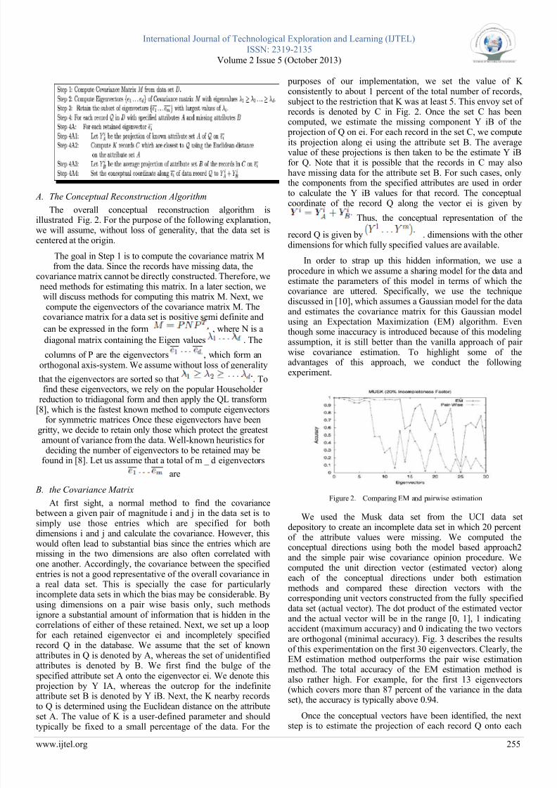
Figure 2. Comparing EM and pairwise estimation

We used the Musk data set from the UCI data setdepository to create an incomplete data set in which 20 percentof the attribute values were missing. We computed theconceptual directions using both the model based approach2and the simple pair wise covariance opinion procedure. Wecomputed the unit direction vector (estimated vector) alongeach of the conceptual directions under both estimationmethods and compared these direction vectors with thecorresponding unit vectors constructed from the fully specifieddata set (actual vector). The dot product of the estimated vector and the actual vector will be in the range [0, 1], 1 indicatingaccident (maximum accuracy) and 0 indicating the two vectorsare orthogonal (minimal accuracy). Fig. 3 describes the resultsof this experimentation on the first 30 eigenvectors. Clearly, theEM estimation method outperforms the pair wise estimationmethod. The total accuracy of the EM estimation method isalso rather high. For example, for the first 13 eigenvectors

(which covers more than 87 percent of the variance in the dataset), the accuracy is typically above 0.94.

Once the conceptual vectors have been identified, the nextstep is to estimate the projection of each record Q onto each




ISSN: 2319-2135


www.ijtel.org 256

abstract vector. In the previous section, we discussed how a setC of close records are determined using the known attributes inorder to perform the rebuilding. We defined C to be the set of records in the neighborhood of Q using the attribute set A. Thevalue for Q is estimated using the records in set C. It is possibleto further refine the performance using the followingobservation.

The values of YB for the records in C may often show somecluster behavior. We cluster the YB values in C in order to

create the sets C1 . . . Cr, where for each set Ci,we compute the distance of its cancroids to the record Q usingthe known attribute set A. The cluster that is closest to Q isused to predict the value of YB. The perception behind thismethod is obvious.

The time complexity of the method can be obtained bysumming the time required for each step of Fig. 2. The firststep is the calculation of the covariance matrix, which normally(when there is no missing data) requires processing time of O(d2. N). For the missing data case, since, essentially, we use theEM procedure to estimate this matrix at each iteration untilconvergence is achieved, the lower bound on the total cost may

be approximated as O(d2 . N. it), where it is the numeral of iterations for which the EM algorithm is run. For a more exactanalysis of the intricacy of the EM algorithm and associatedguarantee of convergence (to a local maximum of the log-likelihood), we refer the reader elsewhere [18], [12]. The

process of Step 2 is simply the generation of the eigenvectorswhich requires a time of O (d3). However, since only m of these eigenvectors needs to be retained, the actual time required

for the combination of Steps 2 and 3 is O . Finally,Step 4 requires m dot product calculations for each record and

requires a total time of O (N.d.m).

II. EMPIRICAL EVALUATIONS

In order to perform the testing, we used several completelyspecified data sets (Musk (1 & 2), BUPA, Wine, and Letter-Recognition) in the UCI3 machine wisdom storehouse. TheMusk 1 data set has 475 instances and 166 dimensions. TheMusk 2 data set has 6,595 instances and 166 dimensions. TheLetter-Recognition data set has 16 dimensions and 20,000instances. The BUPA data set has 6 dimensions and 345instances. The incomplete records were generated by arbitrarilyremoving some of the entries from the records. We introduce anotion of incompleteness in these data sets by arbitrarily

eliminating values in records of the data set. One of theadvantages of this method is that, since we already know theunique data set, we can compare the effectiveness of thereconstruct data set with the actual data set to validate our approach. We use several evaluation metrics in order to test theefficiency of the reconstruction approach. These metrics aredesigned in various ways to test the sturdiness of thereconstructed method in preserve the inherent information fromthe original records.

A. Direct Error Metric

Let be the estimated value of the conceptualcomponent for the eigenvector i using the modernization

method. Let . Be the true value of the projection of

the record Q on to eigenvector i, if we had an oracle whichknew the true projection onto eigenvector i using the original

data set. Obviously, the closer is to

, the better the quality of the reconstruction. We define therelative error5 along the eigenvector i as follows:

Clearly, inferior values of the error metric are moreenviable. In many cases, even when the absolute error inestimation is somewhat high, experiential data suggests that thecorrelation between estimated and actual values continue to bequite high. This indicates that, even though the estimatedconceptual representation is not the same as the truerepresentation, the estimated and actual components arecorrelated so highly that the direct application of many datamining algorithms on the reconstructed data set is likely tocontinue to be effective. To this end, we computed thecovariance and correlation of these actual and estimated

projections for each eigenvector over different values of Q in

the database. A validation of our conceptual

Figure 3. . (a) Error, (b) correlation (estimated, actual), and (c) covariance

(estimated, actual) as a function of eigenvectors for the Musk(1) data set at 20

percent and 40 percent missing

.Rebuilding procedure would be if the correlations between

the actual and estimated projections are high. Also, if the scaleof the covariance between the estimated and actual mechanismalong the principal eigenvectors were high, it would providefurther validation of our intuitions that the principleeigenvectors provide the instructions of the data which have themaximum predictability.

B. Indirect Error Metric

Since the thrust of this paper is to compute conceptualrepresentations for indirect use on data mining algorithmsrather than actual attribute reconstruction, it is also useful toevaluate the methods with the use of an indirect error metric. Inthis metric, we build and compare the performance of a datamining algorithm on the reconstruct data set. To this effect, weuse classifier trees generated from the original data set andcompare it with the performance of the classifier treesgenerated from the reconstructed data set. Let CAo be theclassification accuracy with the original data set and CAr is theclassification accuracy with the reconstructed data set. Thismetric, also referred to as Classification Accuracy Metric(CAM), measures the ratio between the above twoclassification accuracies. More formally:

Thus, the indirect metric measures how close to the originaldata set the reconstructed data set is in terms of classificationaccuracy.

1) Evaluations with Direct Error Metric




ISSN: 2319-2135


www.ijtel.org 257

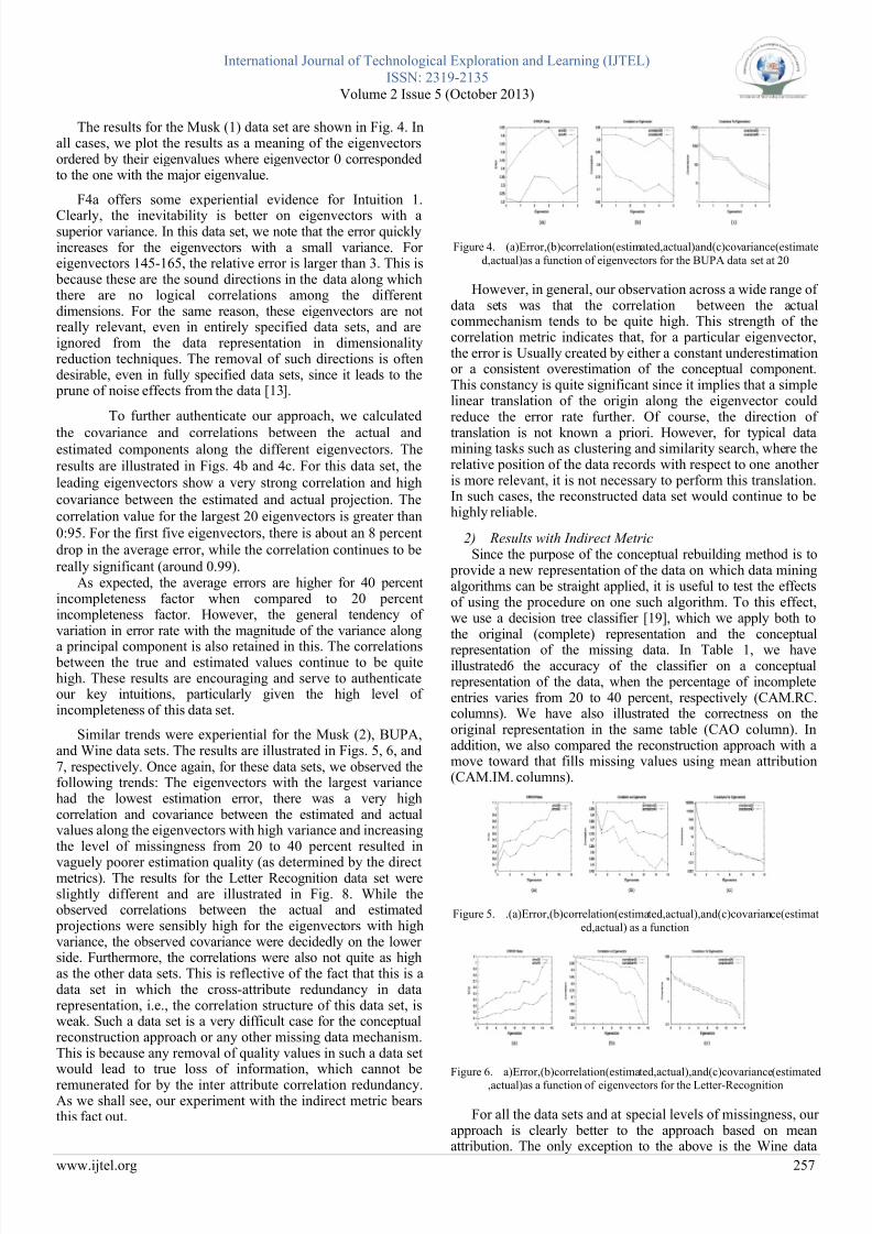
The results for the Musk (1) data set are shown in Fig. 4. Inall cases, we plot the results as a meaning of the eigenvectorsordered by their eigenvalues where eigenvector 0 correspondedto the one with the major eigenvalue.

F4a offers some experiential evidence for Intuition 1.

Clearly, the inevitability is better on eigenvectors with asuperior variance. In this data set, we note that the error quicklyincreases for the eigenvectors with a small variance. For eigenvectors 145-165, the relative error is larger than 3. This is

because these are the sound directions in the data along whichthere are no logical correlations among the differentdimensions. For the same reason, these eigenvectors are notreally relevant, even in entirely specified data sets, and areignored from the data representation in dimensionalityreduction techniques. The removal of such directions is oftendesirable, even in fully specified data sets, since it leads to the

prune of noise effects from the data [13].

To further authenticate our approach, we calculated

the covariance and correlations between the actual andestimated components along the different eigenvectors. Theresults are illustrated in Figs. 4b and 4c. For this data set, the

leading eigenvectors show a very strong correlation and high

covariance between the estimated and actual projection. The

correlation value for the largest 20 eigenvectors is greater than

0:95. For the first five eigenvectors, there is about an 8 percent

drop in the average error, while the correlation continues to be

really significant (around 0.99).As expected, the average errors are higher for 40 percent

incompleteness factor when compared to 20 percentincompleteness factor. However, the general tendency of variation in error rate with the magnitude of the variance along

a principal component is also retained in this. The correlations between the true and estimated values continue to be quitehigh. These results are encouraging and serve to authenticateour key intuitions, particularly given the high level of incompleteness of this data set.

Similar trends were experiential for the Musk (2), BUPA,and Wine data sets. The results are illustrated in Figs. 5, 6, and7, respectively. Once again, for these data sets, we observed thefollowing trends: The eigenvectors with the largest variancehad the lowest estimation error, there was a very highcorrelation and covariance between the estimated and actualvalues along the eigenvectors with high variance and increasingthe level of missingness from 20 to 40 percent resulted in

vaguely poorer estimation quality (as determined by the directmetrics). The results for the Letter Recognition data set wereslightly different and are illustrated in Fig. 8. While theobserved correlations between the actual and estimated

projections were sensibly high for the eigenvectors with highvariance, the observed covariance were decidedly on the lower side. Furthermore, the correlations were also not quite as highas the other data sets. This is reflective of the fact that this is adata set in which the cross-attribute redundancy in datarepresentation, i.e., the correlation structure of this data set, isweak. Such a data set is a very difficult case for the conceptualreconstruction approach or any other missing data mechanism.This is because any removal of quality values in such a data setwould lead to true loss of information, which cannot be

remunerated for by the inter attribute correlation redundancy.As we shall see, our experiment with the indirect metric bearsthis fact out.

Figure 4. (a)Error,(b)correlation(estimated,actual)and(c)covariance(estimate

d,actual)as a function of eigenvectors for the BUPA data set at 20

However, in general, our observation across a wide range of data sets was that the correlation between the actualcommechanism tends to be quite high. This strength of thecorrelation metric indicates that, for a particular eigenvector,the error is Usually created by either a constant underestimationor a consistent overestimation of the conceptual component.This constancy is quite significant since it implies that a simplelinear translation of the origin along the eigenvector couldreduce the error rate further. Of course, the direction of

translation is not known a priori. However, for typical datamining tasks such as clustering and similarity search, where therelative position of the data records with respect to one another is more relevant, it is not necessary to perform this translation.In such cases, the reconstructed data set would continue to behighly reliable.

2) Results with Indirect MetricSince the purpose of the conceptual rebuilding method is to

provide a new representation of the data on which data miningalgorithms can be straight applied, it is useful to test the effectsof using the procedure on one such algorithm. To this effect,we use a decision tree classifier [19], which we apply both tothe original (complete) representation and the conceptual

representation of the missing data. In Table 1, we haveillustrated6 the accuracy of the classifier on a conceptualrepresentation of the data, when the percentage of incompleteentries varies from 20 to 40 percent, respectively (CAM.RC.columns). We have also illustrated the correctness on theoriginal representation in the same table (CAO column). Inaddition, we also compared the reconstruction approach with amove toward that fills missing values using mean attribution(CAM.IM. columns).

Figure 5. .(a)Error,(b)correlation(estimated,actual),and(c)covariance(estimat

ed,actual) as a function

Figure 6. a)Error,(b)correlation(estimated,actual),and(c)covariance(estimated

,actual)as a function of eigenvectors for the Letter-Recognition

For all the data sets and at special levels of missingness, our approach is clearly better to the approach based on meanattribution. The only exception to the above is the Wine data




ISSN: 2319-2135


www.ijtel.org 258

set, where, at 20 percent missingness, the two schemes areequal. In fact, in some cases, the development in accuracy isnearly 10 percent. This improvement is more apparent in datasets where the correlation structure is weaker (Letter-Recognition, Bupa) than in data sets where the correlationstructure is stronger (Musk, Wine data sets). One possiblereason for this is that, although mean imputation often results inincorrect estimations, the stronger correlation structure in theMusk data sets enables C4.5 to ignore the incorrectly estimatedattribute values, thereby ensuring that the classification

performance is relatively unaffected. Note also that theimprovement of our reconstruction approach over meanimputation is more noticeable as we move from 20 percentmissingness to 40 percent missingness. This is true of all thedata sets, including the Wine data set.

For the case of the BUPA, Musk (1), and Musk (2) datasets, the C4.5 classifier built on the reconstructed data set (our approach) was at least 92 percent as correct as the original dataset, even with 40 percent incompleteness. In most cases, theaccuracy was radically higher. This is evidence of the heftinessof the technique and its applicability as a procedure totransform the data without losing the inherent informationavailable in it.

Out of the five data sets experienced, only the letter recognition data set did not show as effective a classification

performance as the other three data sets. This difference isespecially perceptible at the 40 percent incompleteness factor.There are three particular characters of this data set and theclassification algorithm which contribute to this. The firstreason is because the correlation structure of the data set wasnot strong enough to account for the loss of information created

by the missing attributes. Although our approach outperforms

mean imputation, the weak correlation structure of this data settends to amplify the errors of the reconstruction approach. Wenote that any missing data mechanism needs to depend uponinter attribute redundancy and such behavior shows that thisdata set is not as suitable for missing data mechanisms as theother data sets. Second, on presentation the decision trees thatwere constructed, we noticed that, for this particular data set,the classifier happened to pick the eigenvectors with lower variance first, while selecting the splitting attributes. Theselesser eigenvectors also are the ones where our estimation

procedure results in larger errors. This problem may not,however, occur in a classifier in which the higher eigenvectorsare picked first (as in PCA-based classifiers). Finally, in this

particular data set, several of the classes are intrinsically similar to one another and are distinguished from one another by onlysmall variations in their feature values. Therefore, removal of data values has a severe effect on the maintenance of thedistinctive characteristics among different classes. This tends toincrease the misclassification rate.

TABLE I. EVALUTION OF INDIRECT METRIC

We note that, even though the applicability of the generalconceptual reconstruction technique applies across the entire

range of generic data mining problems, it is possible to further improve the method for picky problems. This can be done by

picking or designing the method used to solve that problemmore carefully. For example, we are evaluating strategy bywhich the overall classification performance in suchreconstructed data sets can be improved. As mentioned earlier,one strategy under active consideration is to use class-dependent PCA-based classifiers. This has two advantages:First, since these are PCA-based, our reconstruction approachnaturally fits into the overall model. Second,class-dependentapproaches are typically better discriminators in data sets witha large number of classes and will improve the overallclassification accuracy in such cases. An interesting line of future study would be to develop conceptual reconstructionapproaches which are specially tailored to different data miningalgorithms.

III. CONCLUSIONS AND DIRECTIONS FOR FUTURE

WORK

In this paper, we present the novel idea of theoreticaltransformation for mining particularly incomplete data sets.The key incentive behind conceptual reconstruction is that, bychoosing by prediction the data along the conceptual directions,we use only that level of knowledge that can be reliably

predicted from the incomplete data. This is lither than therestrictive approach of Predicting along the original attributedirections. We show the effectiveness of the technique on awide variety of real data sets. Our results indicate that, eventhough it may not be possible to reconstruct the original dataset for a random feature or vector, the conceptual directions areVery agreeable to reconstruction. Therefore, it is possible toreliably apply data mining algorithms on the conceptualrepresentation of the reconstructed data sets.

In terms of future work, one interesting line is toexpand the proposed ideas to work with categorical attributes.Recall that the current approach works well only on continuousattributes since it relies on PCA. Another motivating avenue of future research could involve investigatingrefinement to theestimation procedure that can improve the efficiency (usingsampling) and accuracy (perhaps by evaluating and using therefinements suggested in Section 3.1) of the conceptualreconstruction procedure.

REFERENCES

[1] C.C. Aggarwal, “On the Effects of Dimensionality Reduction on HighDimensional Similarity Search,” Proc. ACM Symp. Principles of

Database Systems Conf., 2001[2] C.C. Aggarwal and S. Parthasarathy, “Mining Massively Incomplete

Data Sets by Conceptual Reconstruction,” Proc. ACM KnowledgeDiscovery and Data Mining Conf., 2001.

[3] R. Agrawal and R. Srikant, “Privacy Preserving Data Mining,” Pr oc.ACM SIGMOD, 2000

[4] L. Breiman, J.H. Friedman, R.A. Olshen, and C.J. Stone, Classificationand Regression Trees. New York: Chapman & Hall, 1984.

[5] ] A.P. Dempster, N.M. Laird, and D.B. Rubin, “Maximum Likelihoodfrom Incomplete Data via the EM Algorithm,” J. Royal Statistical Soc.Series, vol. 39, pp. 1-38, 1977

[6] A.W. Drake, Fundamentals of Applied Probability Theory. McGraw-Hill, 1967

[7] Z. Ghahramani and M.I. Jordan, “Learning from Incomplete Data,”Dept. of Brain and Cognitive Sciences, Paper No. 108, Massachusetts

Institute of Technology, 1994.

[8] I.T. Jolliffe, Principal Component Analysis. New York: Springer-Verlag, 1986.




ISSN: 2319-2135


www.ijtel.org 259

[9] J. Kleinberg and A. Tomkins, “Applications of Linear Algebra toInformation Retrieval and Hypertext Analysis,” Proc. ACM Symp.Principles of Database Systems Conf., Tutorial Survey, 1999.

[10] R. Little and D. Rubin, “Statistical Analysis with Missing Data Values,”Wiley Series in Probability and Statistics, 1987.

[11] R.J.A. Little and M.D. Schluchter, “Maximum Likelihood Estimate for

Mixed Continuous and Categorical Data with Missing Values,”Biometrika, vol. 72, pp. 497-512, 1985.

[12] ] S.Parthsarthy and C.C. Aggarwal, “On the Use of ConceptualReconstruction for Mining Massively Incomplete Data Sets, “IEEETrans. Knowledge and Data Eng., pp. 1512-1521,2003.

[13] Eclipse Home Page : http://www.eclipse.org/

[14] http://weka.sourceforge.net/wiki/index.php/Writing_your_own_Filter

[15] wekaWikilin :http://weka.sourceforge.net/wiki/index.php/Main_Page

[16] ] Ian H. Witten and Eibe Frank , “Data Mining: Practical MachineLearning Tools and Techniques” Second Edition, Morgan KaufmannPublishers. ISBN: 81-312-0050-7.

[17] http://weka.sourceforge.net/wiki/index.php/CVS

[18] http://weka.sourceforge.net/wiki/index.php/Eclipse_3.0.xweka.filters.SimpleBatchFilter

http://weka.sourceforge.net/wiki/index.php/Writing_your_own_Filter

http://weka.sourceforge.net/wiki/index.php/Eclipse_3.0.x

http://weka.sourceforge.net/wiki/index.php/Eclipse_3.0.x

http://weka.sourceforge.net/wiki/index.php/Writing_your_own_Filter

scheduled theoretical restoration for mining immensely partial data sets

Documents