scene classification processes tina ehtiatidigitool.library.mcgill.ca/thesisfile102975.pdf · scene...
TRANSCRIPT
,~ Strongly Coupled Bayesian Models for Interacting Object and
Scene Classification Processes
Tina Ehtiati
Department ofElectrical and Computer Engineering
Mc Gill University, Montreal
February 2007
A Thesis submitted to the Faculty of Graduate Studies and Research
in partial fulfillment of the requirement for the degree of
Doctor of Philosophy
© TINA EHTIATI, 2007

1+1 Library and Archives Canada
Bibliothèque et Archives Canada
Published Heritage Branch
Direction du Patrimoine de l'édition
395 Wellington Street Ottawa ON K1A ON4 Canada
395, rue Wellington Ottawa ON K1A ON4 Canada
NOTICE: The author has granted a nonexclusive license allowing Library and Archives Canada to reproduce, publish, archive, preserve, conserve, communicate to the public by telecommunication or on the Internet, loan, distribute and sell th es es worldwide, for commercial or noncommercial purposes, in microform, paper, electronic and/or any other formats.
The author retains copyright ownership and moral rights in this thesis. Neither the thesis nor substantial extracts from it may be printed or otherwise reproduced without the author's permission.
ln compliance with the Canadian Privacy Act some supporting forms may have been removed from this thesis.
While these forms may be included in the document page count, their removal does not represent any loss of content from the thesis.
• •• Canada
AVIS:
Your file Votre référence ISBN: 978-0-494-32177-5 Our file Notre référence ISBN: 978-0-494-32177-5
L'auteur a accordé une licence non exclusive permettant à la Bibliothèque et Archives Canada de reproduire, publier, archiver, sauvegarder, conserver, transmettre au public par télécommunication ou par l'Internet, prêter, distribuer et vendre des thèses partout dans le monde, à des fins commerciales ou autres, sur support microforme, papier, électronique et/ou autres formats.
L'auteur conserve la propriété du droit d'auteur et des droits moraux qui protège cette thèse. Ni la thèse ni des extraits substantiels de celle-ci ne doivent être imprimés ou autrement reproduits sans son autorisation.
Conformément à la loi canadienne sur la protection de la vie privée, quelques formulaires secondaires ont été enlevés de cette thèse.
Bien que ces formulaires aient inclus dans la pagination, il n'y aura aucun contenu manquant.

~ 1
Abstract
In this thesis, we present a strongly coupled data fusion architecture within a Bayesian
framework for modeling the bi-directional influences between the scene and object
classification mechanisms. A number of psychophysical studies provide experimental
evidence that the object and the scene perception mechanisms are not functionally
separate in the human visual system. Object recognition facilitates the recognition of the
scene background and also knowledge of the scene context facilitates the recognition of
the individual objects in the scene. The evidence indicating a bi-directional ex change
between the two processes has motivated us to build a computational model where
object and scene classification proceed in an interdependent manner, while no
hierarchical relationship is imposed between the two processes. We propose a strongly
coupled data fusion model for implementing the feedback relationship between the scene
and object classification processes. We present novel schemes for modifying the
Bayesian solutions for the scene and object classification tasks which allow data fusion
between the two modules based on the constraining of the priors or the likelihoods. We
have implemented and tested the two proposed models using a database of natural
images created for this purpose. The Receiver Operator Curves (ROC) depicting the
scene classification performance of the likelihood coupling and the prior coupling
models show that scene classification performance improves significantly in both
models as a result of the strong coupling ofthe scene and object modules.
ROC curves depicting the scene classification performance of the two models also show
that the likelihood coupling model achieves a higher detection rate compared to the prior
coupling mode!. We have also computed the average rise times of the models' outputs as

a measure of comparing the speed of the· two models. The results show that the
likelihood coupling model outputs have a shorter rise time. Based on these experimental
findings one can conclu de that imposing constraints on the likelihood models provides
better solutions to the scene classification problems compared to imposing constraints on
the prior models.
We have also proposed an attentiomil feature modulation scheme, which consists of
tuning the input image responses to the bank of Gabor filters based on the scene class
probabilities estimated by the model and the energyprofiles of the Gabor filters for
different scene categories. Experimental results based on combining the attentional
feature tuning scheme with the likelihood coupling and the prior coupling methods show
a significant improvement in the scene classification performances ofboth models.
11

Résumé
Dans cette thèse, nous présentons une architecture de fusion de données fortement
couplée à l'intérieur d'un cadre bayésien pour la modélisation des influences
bidirectionelles entre les mécanismes de classification de scène et d'objet. Un certain
nombre d'études psychophysiques apportent des preuves expérimentales que les
mécanismes de perception d'objet et de scène ne sont pas séparés fonctionnellement
dans le système visuel humain. La reconnaissance d'objet facilite la reconnaissance de
l'arrière-plan d'une scène et la connaissance du contexte d'une scène facilite aussi la
reconnaissance des objets individuels de la scène. Les preuves indiquant un échange
bidirectionnel entre les deux processus nous ont motivés à construire un modèle
computationnel dans lequel la classification d'objet et de scène procèdent de façon
interdépendante, alors qu'aucune relation hiérarchique n'est imposée entre les deux
processus. Nous proposons un modèle de fusion de données fortement couplé pour
implémenter la relation de feedback entre les processus de classification de scène et
d'objet. Nous présentons de nouvelles techniques pour modifier les solutions
bayésiennes pour les tâches de classification de scène et d'objet qui permettent la fusion
de données entre les deux modules en se basant sur la contrainte des probabilités a priori
ou des vraisemblances. Nous avons implémenté et testé les deux modèles proposés en
utilisant une base de donnée d'images naturelles créés à cet escient. Les courbes de
caractéristique d'opération du récepteur (Receiver Operator Curve - ROC) décrivant la
performance en classification de scène des modèles par couplage de vraisemblance et
par couplage de probabilité a priori montrent que le fort couplage des modules de scène
111

et d'objet resulte en une amélioration significative de la performance en classification de
scène des deux modèles.
Les courbes ROC décrivant la performance en classification de scène des deux modèles
montrent aussi que le modèle par couplage de vraisemblance atteint un taux de détection
plus élevé que le modèle par couplage de probabilité a priori. Nous avons aussi calculé
les temps de montée moyens des sorties des modèles comme mesure de comparaison de
la vitesse des deux modèles. Les résultats montrent que les sorties du modèle par
couplage de vraisemblance ont un temps de montée plus court. En se basant sur ces
résultats expérimentaux, on peut conclure qu'imposer des contraintes sur les modèles
par vraisemblance fournir de meilleures solutions aux problèmes de classification de
scène qu'imposer des contraintes sur les modèles par probabilité a priori.
Nous avons aussi proposé une technique de modulation par trait attentionel qui consiste
au réglage des réponses des images en entrée à la banque de filtres de Gabor en se basant
sur les probabilitées de classes de scènes estimées par le modèle et les profils
energétiques des filtres de Gabor pour différentes catégories de scènes. Des résultats
expérimentaux basés sur la combinaison de la technique de réglage par trait attentionel
avec les méthodes par couplage de vraisemblance et par couplage de probabilité a priori
montrent une amélioration significative de la performance en classification de scène
pour les deux modèles.
iv

Acknowledgements
I would like to express my great gratitude to my supervisor, Dr. James J. Clark, for his
encouragement and guidance throughout my Ph.D. pro gram, and for his time and patience
in the course of writing this thesis. I have been most fortunate to be able to use his wealth
of knowledge and experience as his Ph.D. student during the past four years. I would also
like to thank my thesis committee members, Dr. TaI Arbel and Dr. Michael Langer for
their supervision on my the sis progress.
I would like to thank my friends in the Centre for Intelligent Machines, Wei Sun, Sandra
Skaff, Li Jie, Muhua Li, and Fatima Drissi-Smaili for their companionship which made
my years of Ph.D. studies more fruitful and enjoyable. I thank Vincent Levesque for the
French translation of the abstract ofthis thesis.
My special gratitude goes to my family members, my parents Mohammad Ali Ehtiati and
Servat Rostamkhani, and my husband Zahir Albadawi, for an the support they gave me
throughout my research work.
The research described in this thesis was funded by Precarn Incorporated, as well as
through research grants to the supervisor from the Institute for Robotics and Intelligent
Systems (IRIS).
v

Table of Contents
Chapter 1. Introduction ...................................................................................................... 1
1.1 Motivation ............................................................................................................... 1
1.2 Objectives ................................................................................................................ 3
1.3 Contributions ........................................................................................................... 6
1.4 Overview of the Thesis ............................................................................................ 8
Chapter 2. Cognitive Models of Scene and Contextual Object Perception ..................... 10
2.1 The Content ofthe Gist of a Scene ........................................................................ 12
2.2 Scene Context and Object Perception ................................................................... 15
2.3 Hints from Neurophysiology ................................................................................. 17
2.4 Summary ............................................................................................................... 18
Chapter 3. Computational Models for N atural Scene and Object Classification ............ 21
3.1 Computational Model for Scene Classification ..................................................... 22
3.1.1 Review ofComputational Models for Scene Representation and Classification
................................................................................................................................. 23
3.1.2 Oliva and Torralba Model for Natural Scene Representation and
Classification ........................................................................................................... 28
3.2 Computational Model for Object Classification ................................................... 38
3.2.1 Proposed Object Module Formulation ........................................................... 41
3.3. Summary .............................................................................................................. 45
Chapter 4. Coupling of the Scene Classification Module and the Object Classification
Module ............................................................................................................................. 47
4.1 Data Fusion ............................................................................................................ 47
4.2 Weakly and Strongly Coupled Architectures for Data Fusion .............................. 52
4.3 Strongly Coupled Data Fusion between Scene and Object Modules .................... 57
4.3.1 Adaptive Priors Model ................................................................................... 57
4.3.2 Adaptive Likelihoods Model .......................................................................... 61
Chapter 5. Experimental Results for the Strongly Coupled Scene and Object
Classification Models ...................................................................................................... 64
5.1 Experimental Image Database ............................................................................... 65
5.2 Choice of Model Parameters ................................................................................. 70
5.3 Experimental Results for the Strongly Coupled Scene and Object Modules ........ 72
5.3.1 Case Studies for the Adaptive Priors and Adaptive Likelihood Models ........ 74
5.3.2 Statistical Study of the Classification Results ................................................ 88
Chapter 6. Comparison of the Strongly Coupled Scene and Object Classification Models
......................................................................................................................................... 91
6.1 Classification Performance ofthe Two Models .................................................... 91
6.2 Predictability ofthe Two Models .......................................................................... 92
6.3 Speed of the Two Models ...................................................................................... 97
6.4 Robustness of the Two Models to Input Variations .............................................. 98
Chapter 7. Attentional Feature Tuning .......................................................................... 102
7.1 F eature Tuning Scheme ....................................................................................... 104
7.2 Experimental Results ........................................................................................... 107
Chapter 8. Conclusions and Future Work ..................................................................... 113
8.1 Conclusions ......................................................................................................... 113
8.2 Future Work ........................................................................................................ 116

~. List of Figures
( ) Figure 2.1 Example of a hybrid image used by Oliva and Shyns is shown. The hybrid
images are produced by combining the low frequency components of the amplitude and phase spectra of one scene with the high frequency components of another scene. This ex ample mixes the low frequency component of a city scene with a high frequency component of a highway.(Taken from the paper by Oliva and Schyns [66]) .......................................................................................................................... 14
Figure 2.2 A model is presented where the two mechanisms of scene and object recognition occur in paraIIel, but constantly feedback information to each other so that as soon as there is any information for any possible stages of recognition (scene or object), the model takes advantage of it.. ............................................................. 19
Figure 3.1. (a) Mean power spectrum averaged from 12000 images. (b) Mean power spectra computed for 6000 images of man-made scenes. (d) Mean power spectra of images from natural scenes. (c) and (e) are contour plots of respective power spectra, the contour is chosen so that the sum of the components inside the section represents 50% (and 80%) of the total energy of the spectra. Units are in cycles per pixel. (hnage taken from reference [94]) ................................................................. 28
Figure 3.2. Spectral signatures of 14 different image categories is presented. Each spectral signature is obtained by averaging the power spectra of a few hundred images per category. The contour plots represent 60%, 80%, and 90% of the energy of the spectra. (Taken from reference [95]) ............................................................. 29
Figure 3.3. Coverage of the spatial frequency domain by a bank of24 Gabor filters ...... 31
Figure 3.4. Local patches are extracted from each image using sliding window of different scales. For each local patch of scale Tl, the probability of the presence of
different classes of objects are estimated using likelihood models which are built by patches of the same scale ........................................................................................ 42
Figure 3.5. The scene module creates hypotheses about the identity of the scene based on the global image features and the object module creates hypotheses about the identity of the objects present in the scene based on local image features ............... 46
Figure 4.1 The general architecture of a weakly coupled data fusion model is represented with L sensory information processing modules. The modules are defined on the feature space x , each performing independent sensory information processing tasks represented by functions Il (x), 12 (x), .... The fusion module combines the
results produced by the individual modules to produce a global function represented by j(j) (x),j 2(x), ... ,J L (x» ..................................................................................... 54
./". Figure 4.2 The general architecture of strongly coupled data fusion models are represented, (a) represents a feed forward architecture where the likelihood or the
) prior model of one sensory information processing module is constrained based on the output of another independent functioning module, (b) represents a recurrent architecture where the likelihood or the prior models of both sensory information processing modules are constrained based on output from the other module .......... 55
Figure 5.1 Sample images of the five scene categories are presented. The scene categories presented in each column, from left to right, are street, park, indoors, downtown, and residential scenes ............................................................................ 68
Figure 5.2 Sample images of the five object categories are presented. The object categories presented from top to bottom are people, buildings, cars, furniture, trees . .................................................................................................................................. 69
Figure 5.3. The classification performance for the uncoupled scene model for 60 test images is presented. Each curve shows performance for mixture models with different number of Gaussians. Performance of the model with mixture of 3 Gaussians shows no significance over the performance of model with mixture of 2 Gaussians .................................................................................................................. 71
Figure 5.4. The classification performance for the uncoupled scene model for 60 test images is presented. Each curve shows performance for a different choice of the number of eigenvectors used for the feature extraction process. Performance of the model using 4 eigenvectors shows no significance over the performance of model using 5 or 6 eigenvectors .......................................................................................... 71
Figure 5.5. Percentage of correct classification results for different scene categories averaged for the two coupled methods ..................................................................... 74
Figure 5.6. The scene and object hypotheses created by the first 100 iterations of the two models for a sample image belonging to the residential category are presented, (a) shows the posterior scene probabilities computed by the adaptive priors model, (b) shows the posterior object probabilities computed by the adaptive priors model (c) shows the posterior scene probabilities computed by the adaptive likelihood model, (d) shows the posterior object probabilities computed by the adaptive likelihood model. ....................................................................................................................... 75
Figure 5.7. The scene and object hypotheses created by the first 100 iterations of the two models for a sample image belonging to the residential category are presented, (a) shows the posterior scene probabilities computed by the adaptive priors model, (b) shows the posterior object probabilities computed by the adaptive priors model (c) shows the posterior scene probabilities computed by the adaptive likelihood model, (d) shows the posterior object probabilities computed by the adaptive likelihood model. ....................................................................................................................... 77
Figure 5.8. The scene and object hypotheses created by the first 100 iterations of the two models for a sample image belonging to the street category are presented, (a) shows the posterior scene probabilities computed by the adaptive priors model, (b) shows the posterior object probabilities computed by the adaptive priors model (c) shows the posterior scene probabilities computed by the adaptive likelihood model, (d) shows the posterior object probabilities computed by the adaptive likelihood model. .................................................................................................................................. 80
Figure 5.9. The scene and object hypotheses created by the first 100 iterations of the two models for a sample image belonging to the park category are presented, (a) shows the posterior scene probabilities computed by the adaptive priors model, (b) shows the posterior object probabilities computed by the adaptive priors model (c) shows the posterior scene probabilities computed by the adaptive likelihood model, (d) shows the posterior object probabilities computed by the adaptive likelihood model. .................................................................................................................................. 83
Figure 5.1 o. The scene and object hypotheses created by the first 100 iterations of the two models for a sample image belonging to the downtown category are presented, (a) shows the posterior scene probabilities computed by the adaptive priors model, (b) shows the posterior object probabilities computed by the adaptive priors model (c) shows the posterior scene probabilities computed by the adaptive likelihood model, (d) shows the posterior object probabilities computed by the adaptive likelihood model. ..................................................................................................... 84
Figure 5.11. The scene and object hypotheses created by the first 100 iterations of the two models for a sample image belonging to the indoors category are presented, (a) shows the posterior scene probabilities computed by the adaptive priors model, (b) shows the posterior object probabilities computed by the adaptive priors model (c) shows the posterior scene probabilities computed by the adaptive likelihood model, (d) shows the posterior object probabilities computed by the adaptive likelihood model. ....................................................................................................................... 86
Figure 5.12. The scene and object hypotheses created by the first 100 iterations of the two models for a sample image belonging to the ambiguous category are presented, (a) shows the posterior scene probabilities computed by the adaptive priors model, (b) shows the posterior object probabilities computed by the adaptive priors model (c) shows the posterior scene probabilities computed by the adaptive likelihood model, (d) shows the posterior object probabilities computed by the adaptive likelihood model. ..................................................................................................... 87
Figure 5.13. ROC curves for scene classification results of the test images. (a) ROC curves computed for the coupled priors model. (b) ROC curves computed for the coupled likelihood mode!. Each curve represents results from a fixed iteration ..... 90
Figure 6.1. ROC curves for scene classification results of the coupled likelihood and coupled priors models, (a) ROC curves representing scene classification results from 50th iteration of the two models, (b) ROC curves representing scene classification results from the 150th iteration of the two models ............................. 93
Figure 6.2. Autocorrelation plots for the outputs of the coupled likelihood model, (a) shows the averaged autocorrelations plot of the model outputs which correspond to a correct classification decision, (b) shows the averaged autocorrelations plot of the model outputs which correspond to cases where the scene images remain unclassified or ambiguous ........................................................................................ 95
Figure 6.3. Autocorrelation plots for the outputs of the coupled priors model, (a) shows the averaged autocorrelations plot of the model outputs which correspond to a correct classification decision, (b) shows the averaged autocorrelations plot of the model outputs which correspond to cases where the scene images remain unclassified or ambiguous ........................................................................................ 96
Figure 6.4. Examples ofnoisy images, (a) original image, (b) image with added Gaussian noise of zero mean and 0- =0.1, (c) image with added Gaussian noise of zero mean and Œ=O.OI, (d) image with added Gaussian noise ofzero mean and 0-=0.001...99
Figure 7.l.The Gabor indexes computed for five scene categories, indoors, park, downtown, residential, and street scenes are presented for À, = 8 and e = 0,30,60,90,120,150,180 degrees. Each Gabor index is obtained by averaging the total energy of the database images in each scene category ................................... 105
Figure 7.2. An example of the function of the coupled likelihoods model as combined with feature tuning effect is presented (a) sample input image (b) the probabilities of different objects being present in the scene, as computed by the coupled likelihoods model, without any feature tuning (c) the probabilities of the image belonging to different scene classes, as computed by the coupled likelihoods model, without any feature tuning and (d) the probabilities of the image belonging to different scene classes, as computed by the coupled likelihoods model, combined with feature tuning ................................................................................................. 108
Figure 7.3. An example of the function of the coupled priors model as combined with feature tuning effect is presented (a) sample input image (b) the probabilities of different objects being present in the scene, as computed by the coupled priors model, without any feature tuning (c) the probabilities of the image belonging to different scene classes, as computed by the coupled priors model, without any feature tuning and (d) the probabilities of the image belonging to different scene classes, as computed by the coupled priors model, with feature tuning ................ 109

(
Figure 7.4. (a) ROC curves computed for the coupled likelihood model when combined with top-down feature tuning effect. (h) ROC curves computed for the coupled likelihood model without any feature tuning effect. Each curve represents results for varying decision thresholds for a fixed iteration of the model. .............................. 111
Figure 7.5 (a) ROC curves computed for the coupled priors mode! when combined with top-down feature tuning effect. (b) ROC curves computed for the coupled priors model combined without any feature tuning effect. Each curve represents results for varying decision thresholds for a fixed iteration of the model.. ............................. 112

List of Tables
Table 6.1. Comparison of the speed of the two models using time constants obtained from fitting the model outputs with a first order step response ............................... 97
Table 6.2. Comparison of the speed of the two models using the iteration number in which the model responses rise %63 of the way from their original value at the first iteration, to the value of the threshold ...................................................................... 98
Table 6.3. Classification performance for noisy test images ........................................... 99
Table 6.4. Classification performance for test images with variations in orientation .... 1 01

1. Introduction
Chapter 1
Introduction
1.1 Motivation
Natural scene categorization is one of the most relevant evolutionary tasks of the human
visual system. The great efficiency of this task as perfonned by hum ans has stimulated
much research in the fields of neural physiology, psychophysics, and computational
neuroscience. Contrary to our daily experience of the effortlessness with which natural
scene recognition is performed in humans, this is one of the hardest tasks for machine
vision, and one that the modem state of the art computer vision algorithms have yet to
accomplish. This difficulty is to a great extent due to the vast variability among the
scenes belonging to similar categories of natural scenes. The question of choosing
appropriate scene representations that are capable of capturing the main characteristics of
scene categories without being too sensitive to intra-class variabilities, and are therefore
useful for the scene recognition task, has been the subject of extended research in the
domain of computer vision.
In this work we have looked into the literature in neurophysiology and
psychophysics in order to gain an understanding of how the human visual system
performs scene recognition and categorization and to apply similar models and
mechanisms to the computer vision systems for achieving more efficient scene
recognition capabilities. In this endeavor we have found that the hierarchical view of the
1

1. Introduction
human visual system, which has been supported by neuro-physiological findings, has led
to the general conclusion that understanding the meaning of scenes is a high level visual
task which takes place as the end result of a progressive reconstruction of the retinal
image. The hierarchical architecture of the visual system implies that understanding the
content of local regions of scenes, and recognition of objects in the scene, are the pre
requisite of understanding the meaning of the whole scene. On the other hand we have
found that experimental results in the domain of psychophysics have provided evidence
that scene understanding can take place independently from object recognition. These
results have been interpreted as evidence that sorne sort of high-level abstract
representations of scenes, or "gists" of scenes, are rapidly extracted by the visual system,
bypassing the object recognition stage [76][77]. The low-pass spatial frequency content
of the scenes have been suggested as a candidate for the computational definition of
"gists" since they provide an encoding of the scene that is useful for categorizing scene
information across scene classes. Psychophysical experimental results have furthermore
shown that scene context can be processed and accessed early enough to influence the
recognition of objects. These experiments imply that the abstract conceptual
representations of scenes may be formed before the identification of the objects which
are semantically associated with them.
In general, it is far from being settled what is actually the relationship between
the scene recognition pro cess and object recognition process in the human visual
process, and what actually happens in a brief viewing of a scene. It is still an open debate
in psychophysics whether the objects in the scene are perceived before the scene identity
is produced based on the list of objects and their relations, or the scene context is
2

1. Introduction
grasped independently and perhaps priOf to recognizing objects. But by looking into' the
psychophysical and the neuro-physiological findings one can conc1ude that there is
adequate evidence to suggest that scene and object perception are not unrelated and
disparate mechanisms, but they are correlated and facilitate each other, implying that
they may share computation al resources. Scene-contextual constraint is available early
enough and is robust enough to influence the recognition of objects, and also
identification of the object in a scene promotes the understanding of the meaning of the
scene, implying a bidirectional exchange between the two processes. Our goal in this
thesis is to provide an account of how such a bidirectional influence is computationally
possible. What would be a computational model for implementing the mutual influence
between the two processes?
1.2 Objectives
We would like to build a computational model where the scene recognition and object
recognition mechanisms do not relate to each other in a hierarchical relationship, but
rather ron in parallel. Our objective is to build a computational model where the two
recognition stages occur in paraIlel, but constantly feedback information to each other in
order to enhance the performance of the two processes. The idea is that as soon as there
is any information for any possible levels of recognition, our model takes advantage of
it. In this model an early sensory information extraction stage precedes the semantic
recognition stages. The scene recognition process is performed based on sensory
information from aIl locations in the scene, or "global" scene information. The object
recognition stage is performed based on local sensory information extracted from local
3

1. Introduction
regions in the image. The computational scheme chosen for scene recognition stage must
be capable of eliciting an estimation of the scene identity rapidly and independently of
the object recognition stage, based on the gist type global scene features given to it. The
object module must in parallel produce the most likely candidate interpretations of
individual objects based on local image features. The information inferred by each of the
two recognition processes is projected to the other process, where the set of associations
that corresponds to the relevant content is activated. In implementing such a model the
main questions to address are the following: How are the associations between scenes
and objects represented? How can the results of the scene recognition process become
available to the object recognition process and vise versa?
In this work we propose using strongly coupled data fusion architecture within a
Bayesian framework to model the associations between the scene and the object
recognition mechanisms. The function of each recognition process is modeled using
Bayesian inference methods. The strongly coupled data fusion architecture ensures that
when the a priori constraints built into the scene recognition process and the object
recognition process fail to provide a unique solution for one of the processes, the
knowledge inferred from the other module can be combined as part of the module
estimation process in order to further constrain the solution. Motivated by the strongly
coupled data fusion architecture we present a scheme for modifying the Bayesian
solutions for the scene and the object recognition processes in order to incorporate the
possibility of information sharing between the two processes. The strongly coupled data
fusion architecture allows two approaches to implementing the interactions between the
two modules. In the first approach, the two modules interact through the prior terms of
4

1. Introduction
the Bayesian fonnulation. In this approach the a priori mode1s of the scene and object
modules are modified in order to allow constraints built into the solution process based
on infonnation coming from the other module. This variation of the model is strongly
coupled in tenns of priors. In the second approach, the likelihood models of each module
are refonnulated in order to allow data fusion with the other module. This variation of
the model is strongly coupled in tenns of likelihoods. Both variations of the mode1 we
present are examples of recurrent strongly coupled architecture.
A computational scheme for producing features that capture the context of the
scenes was first proposed by Oliva and Torralba [70]. In their work a holistic
representation of the scene based on oriented bandpass filters is used as the context
features. This image representation encodes spatially localized structural infonnation.
The potential of this representation for serving as features for the computational scene
categorization task has been investigated and demonstrated. Furthennore Torralba and
Oliva [94] have proposed a nove1 Bayesian approach to contextual object detection.
Their approach is based on conditioning the statistics of the low leve1 contextual features
of the scene according to the presence or absence of objects. They show that the scene
contexts can provide an estimate of the likelihood for finding certain classes of objects in
the scene. Murphy et al [65] have further extended this idea and combined the scene
classification and object detection task by maximizing a conditional joint probability
density model that represents the likelihood of different scene classes and the presence of
different object classes in certain locations, as constrained by the global contextual
features.
5

1. Introduction
Our approach has the architectural advantage that the scene identification and
object identification are capable of functioning independently. When one of the
pro cesses does not have enough infonnation in order to create a plausible hypothesis, the
strong coupling data fusion scheme between the two processes can be used in order to
obtain further evidence for creating a hypothesis. Furthennore, our approach is different
from [65) in the sense that we do not just use conditional likelihoods, but rather we use a
full Bayesian fonnulation in which the a priori scene and object models play a crucial
role.
Vi suaI attention is considered to be one of the first and foremost means of
controlling the flow of infonnation between the different levels of visual processing. It
has been shown that the function of attention is tightly associated with object recognition
process in human vision. Numerous studies have probed the function of attention,
demonstrating attentional control over stimuli with complex and conjugate features. In
this work we have investigated the usefulness and efficacy of an attention al process in
the scene recognition process. We have implemented the attentional process for scene
recognition by adding a feature tuning stage in which the high-Ievel infonnation inferred
from the scene recognition pro cess is used to bias image responses to selected spatial
frequency and orientation features that provide higher discrimination for scene
classification task.
1.3 Contributions
The following is a list of the main contributions made in this thesis, most of which have
been published in Ehtiati and Clark [18][19]:
6

1. Introduction
1. We propose a' model in which the process of scene categorization and the
pro cess ofcategorization of individual objects in the scene feedback information to each
other in order to enhance the performance of both processes. The main characteristic of
this model is that the feedback between the two processes is implemented in a way
which allows the two processes to function in parallel, with no hierarchical relationship
being imposed between the two processes. The proposed architecture allows the two
processes to function independently, within their individual required timeframes and
without receiving any feedback from the other process, but as soon as any information is
available by one of the pro cesses it becomes available to the other process through the
feedback connections between the two processes.
2. We propose a strongly coupled data fusion model for implementing the
feedback relationship between the scene categorization and the object categorization
processes. We present a Bayesian interpretation of the strongly coupled data fusion
architecture which allows imposing constraints on either the likelihood models or the
priOf models of the scene and object categorization processes based on feedback from
the other process.
3. We present experimental results which show that the feedback implemented
between the scene categorization and the object categorization processes increases the
performance of scene categorization task. We also investigate the robustness of the
model function to noise and variability in data such as scale and orientation variations.
4. We present a variation of the model in which a top-down attentional
modulation effect from the high-Ievel scene inference process to the lower level scene
feature extraction process is incorporated with the objective of making the scene
7
1. Introduction
categorization process more efficient. In this variation' of the model we use the
hypothesis formed by the scene categorization process to bias global image responses to
selected spatial frequencies and orientations. We show that the effect of combining
feature tuning with the strongly coupled models is to increase the performance of scene
categorization.
1.4 Overview of the Thesis
This thesis is organized as the following. In chapter 2 we examine the CUITent theories
and findings in the domain of cognitive sciences about scene perception and the
relationship between scene perception and object perception, with the goal of motivating
the model presented in this thesis. In chapter 3 we first give a short background on
different computational schemes for scene representation and classification and motivate
and present our choice for the model's formulation of scene classification process. In the
second part of this chapter we discuss briefly different computational schemes for object
representation and classification and motivate and present our choice for the model' s
formulation of object categorization module. In chapter 4 we discuss the implementation
of the feedback between the scene and the object categorization processes. In this
chapter we present the mathematical methodology we have developed through which the
information produced by the two sensory information processing modules, the scene
classification module and the object classification module can become available to each
other and be considered as part of the information processing problem solved in each
module. The methodology we present here is motivated by the field of data fusion. In
this chapter we propose two approaches for implernenting the interactions between the
8

r---..
J. Introduction
scene classification and the object classification modules based on a Bayesian strongly
coupled data fusion architecture, the strongly coupled priors model and the strongly
coupled likelihoods model. In chapter 5 we present the experimental results from the
implementation of the strongly coupled scene and object classification models presented
in chapter 4. We first demonstrate selective examples where the scene module or the
object module cannot perform the scene or the object classification task reliably when
they function independently, but the strong coupling of the two modules improves the
initial classification results. In this chapter we also present the statistical evaluation of
the models performances and address the issue of statistical meaningfulness of the
presented results using receiver operating characteristic (ROC) curves. The statistical
evaluation of the adaptive priors and the adaptive likelihood models provide a basis for
comparing these two models. In this chapter we also give a description of the database
we have created for the purpose of these experiments. In chapter 6 we attempt to
establish the main characteristics of the models such as predictability, speed, and
robustness to input image variations. In chapter 7 we present a variation of the model
which incorporates a top-down attentional feedback from the high-Ievel scene inference
pro cess to the lower level scene feature extraction process. In this chapter we show that
the attentional modulation effect enhances the scene categorization performance.
Chapter 8 provides conclusion for the CUITent work and suggestions for future work.
9

2. Cognitive Models of Scene and Contextual Object Perception
Chapter 2
Cognitive Models of Scene and Contextual Object Perception
We often take our ability to quickly and accurately understand real-world scenes for
granted. It is normal for us to be able to rapidly grasp the meaning of different scenes
while scanning through different channels on the TV, the downtown of Montreal with
high buildings and people and cars moving around, a courtroom full of people and
fumiture, a boat sailing in the sea, etc. We are able to efficiently and accurately
recognize and categorize the new scene types without our visual system requiring
significant amounts of time to adjust and tune itself.
The rapid apprehension of the world by the human visual system has been the
subject of many psychophysical studies. Potter et al. utilized rapid seriaI vi suai
presentations (RSVP) of images to find out that subjects could understand a visual scene
with exposures of as brief as 100 ms, and might be able to extract semantic information
about scene context from presentations as brief as 80 ms [76][77]. Furthermore, they
demonstrated that while the semantic information of a scene is quickly extracted, it
requires a few hundred milliseconds (about 300 ms) to be consolidated into memory.
These results have been interpreted as evidence that a high-Ievel abstract representation
of the visual scene, which can be accessed very rapidly, is continually generated by the
visual system. This representation, which is called the "gist" of a scene, is defined as a
conceptual summary of the principal semantic features of the scene as perceived in a
brief viewing. In other words, the gist of the scene is the conceptual content of the scene
10
2. Cognitive Models ofScene and Contextual Object Perception
understood in a glance. In experiments performed by Standing et al [86] and Standing
[87] it is shown that our visual memory performs very well in identifying scenes viewed
previously among very large sets of old and new scenes. One possible explanation of this
performance can be that in this task only the gist of the scenes are required for
recognition of old scenes.
Sorne evidence for abstract representations of scenes also cornes from the
phenomenon of boundary extension [46] [3 5]. Boundary extension is a type of memory
distortion in which observers report having seen not only information that was physically
present in the scene, but also information that they have extrapolated outside the scene's
boundaries. Similarly, in visual false memory experiments, participants report that they
remember having seen, in a previously presented picture, objects that are contextually
related to that scene but that were not in the picture. Such memory distortions might be
the byproduct of an efficient mechanism for extracting and encoding the gist of a scene.
It is interesting to compare the capacity of our brain for holding gist of scenes with its
capacity to hold details of objects in scenes. The limits of our perception of objects
during RSVP experiments has been studied by Rensink et al.[80] and O'Regan et al
[73]. They used the "mud splash" technique ofmasking a change in the scene by making
several simultaneous conspicuous changes at different locations in the scene (similar to
the effect of a mud splash on a car windscreen). They show that when the attentional
effect introduced by visual transients accompanying a change in the scene is masked,
changes to retinotopically large portions of the scene sometimes can fail to be detected
by viewers. This is more likely to occur when the regions are not linked to the scene's
overall meaning. This striking phenomenon has been termed "change blindness". The
11

2. Cognitive Models ofScene and Contextual Object Perception
phenomenon of change blindness is especially interesting since it challenges the view of
the "picture in the head", or an exact and detailed internaI representation of the visual
world in our brain, which is usually assumed in the passive vision theories. Change
blindness is better explained when the active vision perspective is adopted. O'Regan et
al [72] show that for objects directly fixated change detection ability is high.
2.1 The Content of the Gist of a Scene
Other investigators have attempted to elucidate the nature of infonnation captured by the
gist of a scene. What is the nature of infonnation that we perceive and understand when
we rapidly glance at the world?
Mandler and Parker have suggested that three types of information are
remembered from a picture: i) an inventory of objects, ii) descriptive information of the
physical appearance and other details of the objects, iii) spatial relationships between the
objects [58]. Freidman and colleagues proposed that early scene recognition involves the
identification of at least one obligatory object [30]. In their model, the obligatory object
serves as a contextual pivotaI point for the recognition of other parts of the scene. They
have also provided evidence that objects can be recognized independently, without
facilitation by the global scene context. Bar and Ullman [3] show that an ambiguous
object becomes recognizable when another object that is contextually associated with it,
is placed in an appropriate spatial relation to it.
On the other hand, other researchers have supported the idea that early scene
processing is based on global scene information rather than local object information.
Wolfe speculates that the spatiallayout ofthe scene and a general impression of the low-
12

,r-..
2. Cognitive Models of Scene and Contextual Object Perception
level features that fill the scene (e.g., texture, etc.) contribute to the understanding of the
conceptual content of a scene [108]. Metzger and Antes [62] show that contextual
information is extracted before observers can saccade towards the portions of the picture
that were rated as contributing most to the context of the scene, and possibly even before
the recognition of individual objects. Loftus et al [56] furthermore show that observers
process the most informative portions of an image earliest.
Biederman et al. [5] found that recognition of objects is impaired when the
objects are embedded in a randomly jumbled scene rather than a coherent scene.
Biederman' s finding implies that sorne kind of global context of the scene is registered
in the early stages of scene perception, which can modulate the object recognition
mechanism. His conclusions regarding scene perception parallel concepts in the auditory
studies of sentence and word comprehension. He suggests using an analogy with analysis
of language material, that scenes could be regarded as schemas, providing a frame in
which objects are viewed. He identifies several physical (support, interposition) and
semantic (probability, position, size) constraints, which objects must satisfy within a
scene, similar to the syntactic and grammatical rules of language [6]. He shows that
scenes with typical physical and structural regularities which follow contextual semantic
rules facilitate object recognition as compared to scenes where these rules and
regularities are violated.
Boyce et al. [9] have demonstrated that objects are more difficult to identify
when Iocated against a contextually inconsistent background, given a briefly flashed
scene (150 ms) as compared with the effect of a meaningless background that was
equated for visual appearance.
13
2. Cognitive Models of Scene and Contextual Object Perception
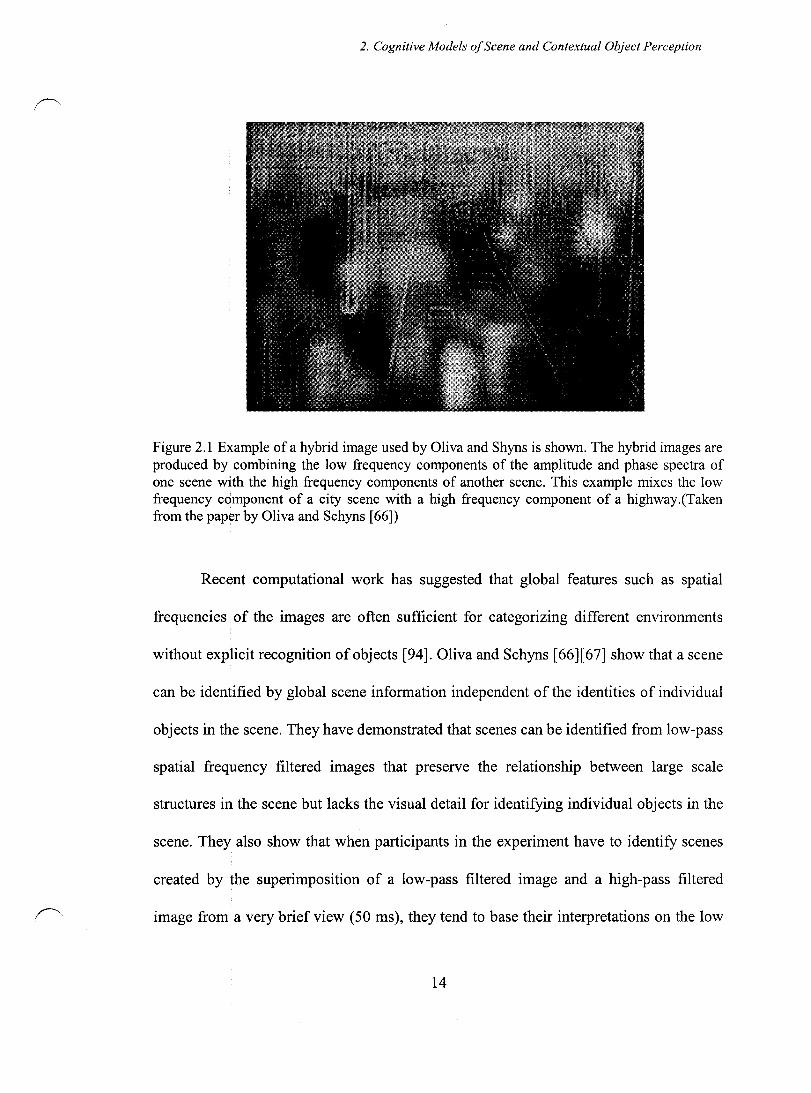
Figure 2.1 Example of a hybrid image used by Oliva and Shyns is shown. The hybrid images are produced by combining the low frequency components of the amplitude and phase spectra of one scene with the high frequency components of another scene. This example mixes the low frequency component of a city scene with a high frequency component of a highway.(Taken from the paper by Oliva and Schyns [66])
Recent computational work has suggested that global features such as spatial
frequencies of the images are often sufficient for categorizing different environments
without explicit recognition of objects [94]. Oliva and Schyns [66][67] show that a scene
can be identified by global scene information independent of the identities of individual
objects in the scene. They have demonstrated that scenes can be identified from low-pass
spatial frequency filtered images that preserve the relationship between large scale
structures in the scene but lacks the visual detail for identifying individual objects in the
scene. They also show that when participants in the experiment have to identify scenes
created by the superimposition of a low-pass filtered image and a high-pass filtered
image from a very brief view (50 ms), they tend to base their interpretations on the low
14

2. Cognitive Models of Scene and Contextual Object Perception
frequency information rather than the high frequency information. This interpretation for
gist of scenes is specifically interesting in the light of the experimental results of HubeI
and Weisel [45] which provide evidence for the presence of oriented band-pass filters at
the early stages of the visual pathway. An example of the superimposed images used by
Oliva and Schyns is shown in figure (2.1).
2.2 Scene Context and Object Perception
Sorne discrepancies appear to exist between the different theories and experimental
results described in section 2.1. Although intuitively much of the meaning of a scene is
defined by the objects that comprise the scene (it is hard to imagine a scene that does not
contain any objects), there is evidence that it is possible to produce a "gist" of a scene
independent of constituent objects, and furthermore this "gist" modulates object
recognition. On the other hand there is evidence from the experiments that at least sorne
sort of object recognition is present even in the early stages of scene perception. At least
sorne objects are recognized in the brief viewings of c1uttered scenes. So the question
which arises is that are the objects in the scene perceived first, and then the scene
identity is produced based on the list ofthese objects and their relations? Or is the scene
context grasped independently, and perhaps prior to recognizing objects? How are the
two perceptions related? 1s object recognition part of early scene perception? These
questions have been the topic of an open debate by the psychophysical community for
more than two decades [33][16][41].
The perceptual schema model proposes that expectations derived from
knowledge about the composition of a scene type interact with the perceptual analysis of
15

2. Cognitive Models ofScene and Contextual Object Perception
objects in the scene [62][5][6][74]. This model is supported by studies of scene
consistencyand object detection. This view suggests that scene context infonnation can
be processed and accessed early enough to influence recognition of objects contained in
the scene, even inhibiting recognition of inconsistent on es [7]. The priming model, on
the other hand, proposes that the locus of the contextual effect is at the stage where a
structural description of an object is matched against long-tenn memory representations
[30][3]. This model suggests that the activation of a certain scene context primes the
stored representations of context-consistent object types, and facilitates convergence to
the most likely interpretations during the object recognition process. This model implies
a definition of scene context independent of the identity of the objects semantically
associated with the scene.
Regardless of the mechanism, both the priming model and the perceptual schema
model c1aim that scene context facilitates consistent objects more than inconsistent ones.
These theories predict that we should observe a correlation of object identification
perfonnance with scene context categorization perfonnance [22]. In contrast, a third
theory called the functional isolation model, proposes that object identification is
isolated from expectations derived from scene knowledge [40]. Henderson and
colleagues, who propose this view, predict that experiments examining the perceptual
analysis of objects should find no systematic relation between object and scene
recognitionperfonnance. Hollingworth and Henderson [40] mention that whereas
objects tend to have a highly constrained set of component parts and relations between
parts, a scene places far less constraint on objects and spatial relationship among objects.
16

2. Cognitive Models ofScene and Contextual Object Perception
2.3 Hints from N europhysiology
The ventral visual pathway, linking the primary visual cortex through inferior temporal
cortex to the pre frontal cortex, is generally known as the "what" visual pathway, as it is
responsible for object recognition through integrating features [101][50][64][98]. Given
the hierarchical structure of the visual system many have proposed models in which the
elementary features of the objects are first processed and then bound together for object
recognition [96][107]. Although many studies have revealed the cortical mechanisms
involved in the recognition of individual objects, in comparison little work has been
done to reveal the neural underpinnings of scene perception and contextual object
recognition. Neuro-imaging studies have shown that a region in the parahippocampal
cortex (PHC) responds preferentially to topographical information and spatial
landmarks, the Parahippocampal place area (PPA) [1][21][57]. This region has an
important role in large scale integration [54] and is increasingly being speculated to be a
module for scene analysis [20][88]. Experimental results have also shown that objects
may be grouped by physical appearance in the occipital visual cortex [36][91], by basic
level categories in the anterior temporal cortex [78][39][17], by contextual relations in
the parahippocampal cortex (PHC) [4], and by semantic relations in the prefrontal cortex
(PFC) [31]. Bar has performed experiments in order to investigate the cortical areas
involved during a contextual processing [4]. He designed experiments in which he
compares the fMRI signal elicited during the recognition ofvisual objects that are highly
associated with a certain context with that elicited by objects that are not associated with
any unique context. He reports that the largest focus of differential activity is in the
posterior PRC, which is the site that encompasses pp A. The other foci of activation are
17
2. Cognitive Models ofScene and Contextual Object Perception
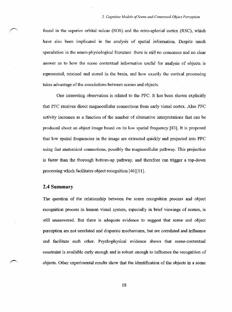
found in the superior orbital sulcus (SOS) and the retro-splenial 'cortex (RSC), which
have also been implicated in the analysis of spatial information. Despite much
speculation in the neuro-physiological literature there is still no consensus and no clear
answer as to how the scene contextual information useful for analysis of objects is
represented, retained and stored in the brain, and how exactly the cortical processing
takes advantage ofthe associations between scenes and objects.
One interesting observation is related to the PFC. It has been shown explicitly
that PFC receives direct magnocellular connections from early visual cortex. Aiso PFC
activity increases as a function of the number of alternative interpretations that can be
produced about an object image based on its low spatial frequency [83]. It is proposed
that 10w spatial frequencies in the image are extracted quickly and projected into PFC
using fast anatomical connections, possibly the magnocellular pathway. This projection
is faster than the thorough bottom-up pathway, and therefore can trigger a top-down
processing which facilitates object recognition [46][11].
2.4 Summary
The question of the relationship between the scene recognition process and object
recognition process in human visual system, especially in brief viewings of scenes, is
still unanswered. But there is adequate evidence to suggest that scene and object
perception are not unrelated and disparate mechanisms, but are correlated and influence
and facilitate each other. Psychophysical evidence shows that scene-contextual
constraint is available early enough and is robust enough to influence the recognition of
objects. Other experimental results show that the identification of the objects in a scene
18

2. Cognitive Models of Scene and Contextual Object Perception
promotes the understanding of the meaning of the scene. One can hypothesize that there
is a bidirectional ex change of information between the two processes, without one
pro cess being necessarily pre-requisite of the other. Our goal in this thesis is to provide
an account of how such a bidirectional influence is computationally possible while
retaining biological plausibility. What would be a computational model for
implementing the mutual influence between the two processes?
Global Image Features
Scene Module
Hypothesis generated: Scene identity
Local Image Features
Object Module
Hypothesis generated: Objects present in the scene
Figure 2.2 A model is presented where the two mechanisms of scene and object recognition occur in parallel, but constantly feedback information to each other so that as soon as there is any information for any possible stages of recognition (scene or object), the model takes advantage of it.
In figure (2.2) we present the general architecture of the model we propose for
implementing the bi-directional relationship between the scene recognition and the
object recognition process. The model consists of two modules, the scene module and
the object modules, which encapsulate the process of scene recognition and object
recognition. The main characteristic of this model is that the scene recognition and
19

2. Cognitive Models ofScene and Contextual Object Perception
object recognition mechanisms do not relate to each other in a hierarchical relationship,
but rather run in parallel. The model has to be implemented in a fashion that although the
two pro cesses occur in parallel, they constantly feedback information to each other in
order to enhance the performance of the two processes. In the next chapter we discuss
the computational formulation for each of the two modules.
20

3. Computation al Models for Natural Scene and Object Classification
Chapter 3
Computational Models for Natural Scene and Object Classification
In the previous chapter we examined the current theories and findings in the domain of
cognitive sciences about scene perception and the relationship between scene perception
and object perception. We explained that, contrary to seminal approaches to vision
which viewed scene perception as a result of a hierarchical visual organization, there is
strong evidence that scenes can be understood very rapidly and independently of the
recognition of the constituent objects. We found that there is strong psychophysical
evidence that the two processes of scene perception and object perception are correlated,
with the results of each process affecting and constraining the outcome of the other
process. This motivates us to investigate the possibility of computational
implementation of a model which incorporates this bi-directional relationship.
Our goal is not to build a high performance scene classification or object
classification model per se; but to build a model which allows the two processes to
interact with each other, and see if such an interaction entails any significant increase in
the scene and object classification performance compared to an implementation with no
feedback. As mentioned previously our proposed model has two modules for scene
classification and object identification, which are able to function either independently or
with feedback, based on availability of information from the other module. In this
chapter we discuss the formulation of each of the modules as they function separately. In
section 3.1 we first give a short background on different computational schemes for
21

3. Computational Models for Natural Scene and Object Classification
scene representation and classification and motivate our choice for the model's
formulation for scene classification. In section 3.2 we discuss briefly different
computational schemes for object representation and classification and motivate our
choice of formulation of the mode!' s object module. In the following chapter we will
continue the discussion with the implementation of the feedback between the two
modules.
3.1 Computational Model for Scene Classification
The scene classification problem is one of the most challenging problems in computer
vision. Given an arbitrary scene, we would like to describe it as belonging to a
semantically meaningful category. A complete approach to scene classification should
address the issues of feature selection (scene representation), feature organization, and
classification. One computational approach to scene representation and classification is
to view it as a process that combines low level image features (col or, orientation, texture,
etc.) to form progressively higher level constructs su ch as regions, geons, objects, and
finally complex scenes. This approach is motivated by the hierarchical view of the visual
system where at the earliest stage from retina to V 1 simple features such as lines and
edges are processed, in visu al cortex V 4 more complex features su ch as curve contours
or 3D orientations are being processed. CeUs responding to complex object patches are
found in the anterior regions of IT, and finally in PPA layout of scenes are processed.
This approach to human vision has been challenged by recent findings in psychophysics
which suggest that scene understanding can happen independently from object
recognition (see the discussion found in chapter 2). In parallel, a new computational
22

3. Computational Modelsfor Natural Scene and Object Classification
approach to scene representation and classification has been developed which processes
low level features directly without the creation of intermediate progressive levels of
abstraction. In the following section we briefly review sorne of the more recent work in
this area in order to motivate our choice of scene representation and scene classification
method.
3.1.1 Review of Computational Models for Scene Representation and Classification
A number of recent studies have presented approaches to classify scene images using
global eues (e.g. power spectrum, color histogram information). Gorkani and Picard [34]
discriminate between photos of city scenes and photos of landscape scenes using a
multiscale steerable pyramid to find dominant orientations in 4x4 sub-blocks of the
image. The image is classified as a city scene if enough sub.,blocks have strong dominant
vertical orientations, or alternatively medium-strong vertical orientation and also
horizontal orientation. Yiu [110] uses the same dominant orientation features and also
color information, to classify indoor and outdoor scenes using nearest neighbor and
support vector machine classifiers. Szummer and Picard [90] combine color histogram
features and DCT -based features capturing shift invariant intensity variations over a
range of scales to discriminate between indoor and outdoor images. They report that k-
nearest neighborhood classifiers perforrned as weIl as more sophisticated classification
methods such as neural networks. They deal with the problem of combining local and
global properties through a multi-stage classification method. They divide the images
into sub-block and classify the sub-blocks independently and then perforrn another stage
of classification on these results for the image as a whole. The disadvantage of this
23
3. Computational Models for Natural Scene and Object Classification
method is that spatial location information is not used for classification of sub-blocks;
therefore the individual sub-block classifiers are less accurate than the whole image
classifier.
Carson et al [13] propose a representation of images based on blobs. Each blob is
a coherent color-texture region. AIl the blobs in aIl image categories are clustered into a
set of canonical blobs using Gaussian models. Each image is thenassigned a score
vector which measures the nearest distance of each canonical blob to the image. These
score vectors are used to train a classifier.
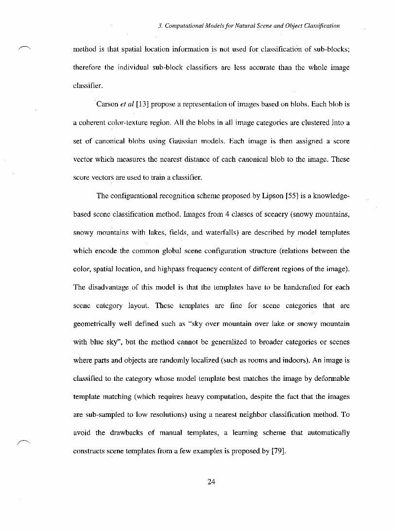
The configurational recognition scheme proposed by Lipson [55] is a knowledge
based scene classification method. Images from 4 classes of scenery (snowy mountains,
snowy mountains with lakes, fields, and waterfalls) are described by mode! templates
which encode the common global scene configuration structure (relations between the
color, spatial location, and highpass frequency content of different regions of the image).
The disadvantage of this model is that the templates have to be handcrafted for each
scene category layout. These templates are fine for scene categories that are
geometrically weIl defined such as "sky over mountain over lake or snowy mountain
with blue sky", but the method cannot be generalized to broader categories or scenes
where parts and objects are randomly localized (such as rooms and indoors). An image is
classified to the category whose model template best matches the image by deformable
template matching (which requires heavy computation, despite the fact that the images
are sub-sampled to low resolutions) using a nearest neighbor classification method. To
avoid the drawbacks of manu al templates, a learning scheme that automatically
constructs scene templates from a few examples is proposed by [79].
24
3. Computational Models for Natural Scene and Object Classification
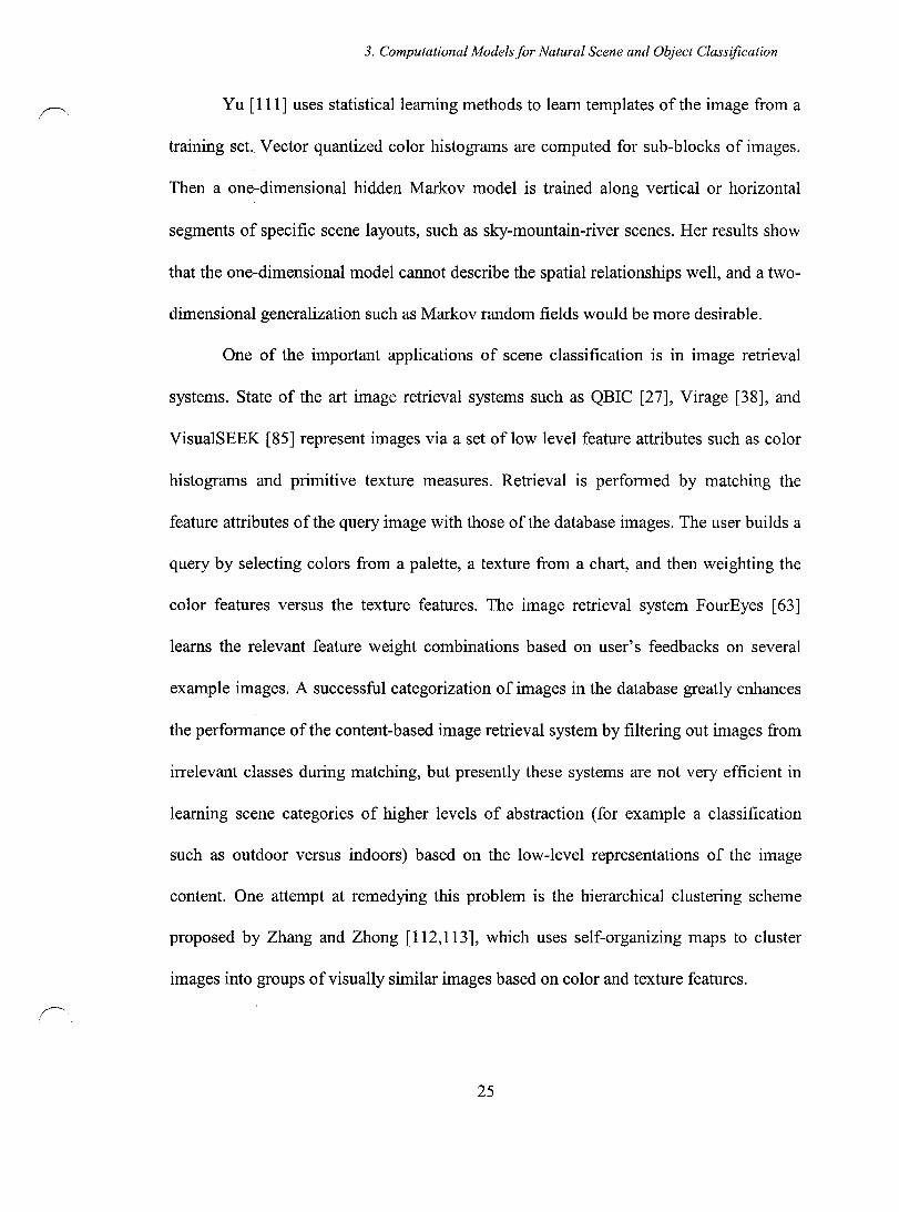
Yu [111] uses statisticalleaming methods to leam templates of the image from a
training set. Vector quantized color histograms are computed for sub-blocks of images.
Then a one-dimensional hidden Markov model is trained along vertical or horizontal
segments of specific scene layouts, such as sky-mountain-river scenes. Rer results show
that the one-dimensional model cannot describe the spatial relationships well, and a two
dimensional generalization such as Markov random fields would be more desirable.
One of the important applications of scene classification is in image retrieval
systems. State of the art image retrieval systems such as QBIC [27], Virage [38], and
VisualSEEK [85] represent images via a set of low level feature attributes such as color
histograms and primitive texture measures. Retrieval is performed by matching the
feature attributes of the query image with those of the database images. The user builds a
query by selecting colors from a palette, a texture from a chart, and then weighting the
color features versus the texture features. The image retrieval system FourEyes [63]
leams the relevant feature weight combinations based on user' s feedbacks on several
example images. A successful categorization of images in the database greatly enhances
the performance of the content-based image retrieval system by filtering out images from
irrelevant classes during matching, but presently these systems are not very efficient in
leaming scene categories of higher levels of abstraction (for example a classification
such as outdoor versus indoors) based on the low-level representations of the image
content. One attempt at remedying this problem is the hierarchical clustering scheme
proposed by Zhang and Zhong [112,113], which uses self-organizing maps to cluster
images into groups ofvisually similar images based on color and texture features.
25
(~
3. Computational Models for Natural Scene and Object Classification
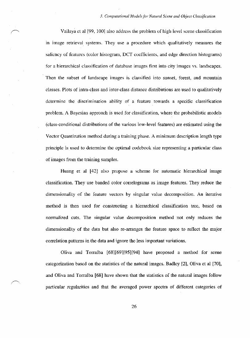
Vailaya et al [99, 100] also address the problem of high level scene classification
ln image retrieval systems. They use a procedure which qualitatively measures the
saliency of features (color histogram, DCT coefficients, and edge direction histograms)
for a hierarchical classification of database images first into city images vs. landscapes.
Then the subset of landscape images is classified into sunset, forest, and mountain
classes. Plots of intra-class and inter-class distance distributions are used to qualitatively
determine the discrimination ability of a feature towards a specific classification
problem. A Bayesian approach is used for classification, where the probabilistic models
(class-conditional distributions ofthe various low-Ievel features) are estimated using the
Vector Quantization method during a training phase. A minimum description length type
principle is used to determine the optimal codebook size representing a particular class
of images from the training samples.
Huang et al [42] also propose a scheme for automatic hierarchical image
classification. They use banded color correlograms as image features. They reduce the
dimensionality of the feature vectors by singular value decomposition. An iterative
method is then used for constructing a hierarchical classification tree, based on
normalized cuts. The singular value decomposition method not only reduces the
dimensionality of the data but also re-arranges the feature space to reflect the major
correlation patterns in the data and ignore the less important variations.
Oliva and Torralba [68][69][95][94] have proposed a method for scene
categorization based on the statistics of the natural images. Badley [2], Oliva et al [70],
and Oliva and Torralba [68] have shown that the statistics of the natural images follow
particular regularities and that the averaged power spectra of different categories of
26

3. Computational ModelsforNatural Scene and Object Classification
scenes exhibit different orientation and spatial frequency distributions. They have used
spatial frequency and orientation tuned filters to create a representation of scenes based
on their characteristic power spectra.
Our design goal to avoid a hierarchical relationship between the object and the
scene modules constrains us to choose a model which adopts a direct scene
representation approach as opposed to a hierarchical scene representation. The model
proposed by Oliva and Torralba captures the main insights which the other models in
line with the direct scene representation, such as Gorkani and Picard [34], Szummer and
Picard [90], and Vailaya et al [99][100] offer. In terms of scene feature selection,
sampling of the low frequency content of the scene power spectra using a bank of Gabor
filters is founded on the psychophysical findings which provide evidence for scene
recognition based on low frequency content of images. These features capture multi
scale information from images, similar to multi-scale steerable pyramids and DCT based
features, and can be computed in parallel over the whole image. In fact, Oliva has
proposed that these features can serve as a computational account for "gist" features,
since based on them the scenes can be rapidly and directly be identified [71]. In terms of
feature organization, Oliva and Torralba use principal components analysis (PCA) for
maximizing variability among features of different classes. The method proposed by
Oliva and Torralba is successful in categorizing scenes at basic level classes, such as
street, buildings, highways, and beach scenes, which is not achieved by the other
methods. Motivated by this discussion we have based our formulation of the scene
module based on the work of Oliva and Torralba; therefore, we present a detailed
discussion of their model in the following section.
27
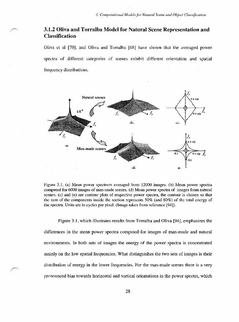
3. Computational Models for Natural Scene and Object Classification
3.1.2 Oliv·a and Torralba Model for Natural Scene Representation and Classification
Oliva et al [70], and Oliva and Torralba [68] have shown that the averaged power
spectra of different categories of scenes exhibit different orientation and spatial
frequency distributions.
Figure 3.1. (a) Mean power spectrum averaged from 12000 images. (b) Mean power spectra computed for 6000 images of man-made scenes. (d) Mean power spectra of images from natural scenes. (c) and (e) are contour plots of respective power spectra, the contour is chosen so that the sum of the components inside the section represents 50% (and 80%) of the total energy of the spectra. Units are in cycles per pixel. (Image taken from reference [94]).
Figure 3.1, which illustrates results from Torralba and Oliva [94], emphasizes the
differences in the mean power spectra computed for images of man-made and natural
environments. hl both sets of images the energy of the power spectra is concentrated
mainly on the low spatial frequencies. What distinguishes the two sets of images is their
distribution of energy in the lower frequencies. For the man-made scenes there is a very
pronounced bias towards horizontal and vertical orientations in the power spectra, which
28

3. Computational Modelsfor Natural Scene and Object Classification
can be explained by the fact that in man-made environments the structural elements of
the scene are organized mainly in horizontal or vertical layers. The power spectra of the
natural scenes have a tendency to be more isotropic as compared to the man-man made
scenes, but still there is a more energy concentrated on the vertical spatial frequencies, as
a lot of natural scenes are organized along layers parallel to the horizon.
® <ê> @ @ ~ ~ t Nalurul River and Forest Mountafn Field Beach Coast ooject walertall
<$> ® +. +-+ ~ Man-made Portrait Jndoor Street tligb City-vlew Highway
objeet sœrre building
Figure 3.2. Spectral signatures of 14 different image categories is presented. Bach spectral signature is obtained by averaging the power spectra of a few hundred images per category. The contour plots represent 60%, 80%, and 90% of the energy of the spectra. (Taken from reference [95])
Figure 3.2, which illustrates results from Torralba and Oliva [95], shows the
spectral signatures of 14 different categories of scenes. One striking result is that basic
level classes of scenes such as streets, highways, buildings, and indoor scenes have
typical spectral signatures. The difference among the spectra of various man-made
categories lies in the relationship between the horizontal and vertical contours at
different spatial scales. On the other hand, the spectra of the natural scenes exhibit a
broader range of variations. Large scale scene categories dominated by the horizon, have
a high percentage of the energy concentrated on the vertical orientation, but in scenes
29
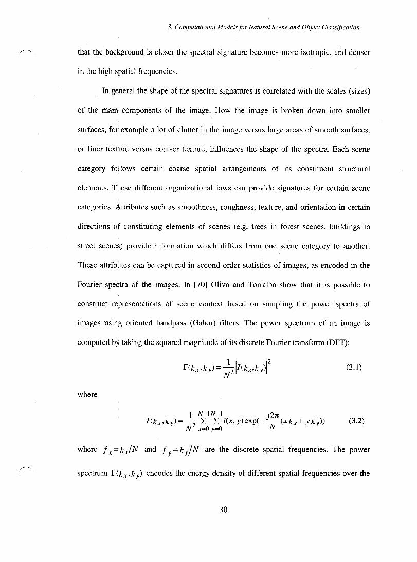
3. Computational Modelsfor Natural Scene and Object Classification
that the background is closer the spectral signature becomes more isotropic, arid denser
in the high spatial frequencies.
In general the shape of the spectral signatures is correlated with the scales (sizes)
of the main components of the image. How the image is broken down into smaller
surfaces, for ex ample a lot of clutter in the image versus large areas of smooth surfaces,
or finer texture versus coarser texture, influences the shape of the spectra. Each scene
category follows certain coarse spatial arrangements of its constituent structural
elements. These different organizational laws can provide signatures for certain scene
categories. Attributes su ch as smoothness, roughness, texture, and orientation in certain
directions of constituting elements of scenes (e.g. trees in forest scenes, buildings in
street scenes) pro vide information which differs from one scene category to another.
These attributes can be captured in second order statistics of images, as encoded in the
Fourier spectra of the images. In [70J Oliva and Torralba show that it is possible to
construct representations of scene context based on sampling the power spectra of
images using oriented bandpass (Gabor) filters. The power spectrum of an image is
computed by taking the squared magnitude of its discrete Fourier transform (DFT):
(3.1)
where
1 N-IN-l j2Jr I(k x ,kY)=2 L L i(x,y)exp(--N (xkx+Yk y» (3.2)
N x=Oy=O
where f x = k xl N and f y = k y / N are the discrete spatial frequencies. The power
spectrum r(k x ' k y) encodes the energy density of different spatial frequencies over the
30
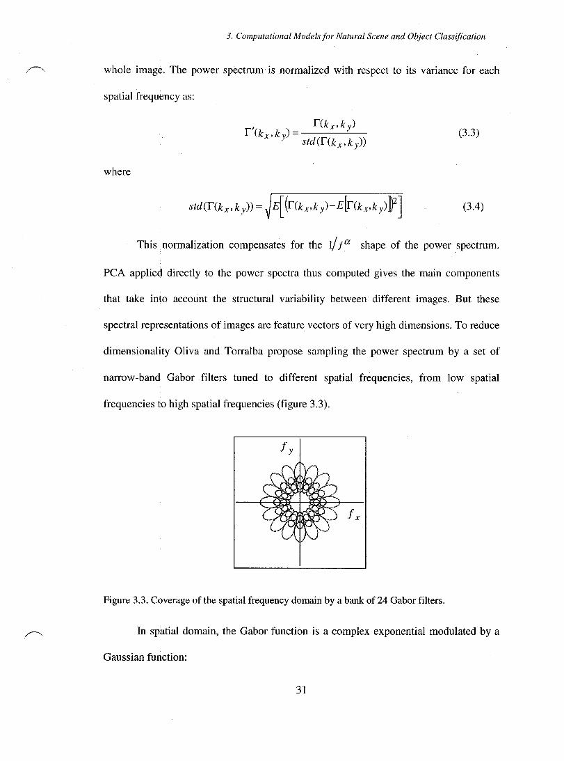
3. Computational Modelsfor Natural Scene and Object Classification
whole image. The power spectrum is normalized with respect to its variance for each
spatial frequency as:
(3.3)
where
(3.4)
This normalization compensates for the 1/ fa shape of the power spectrum.
PCA applied directly to the power spectra thus computed gives the main components
that take into account the structural variability between different images. But these
spectral representations of images are feature vectors of very high dimensions. To reduce
dimensionality Oliva and Torralba propose sampling the power spectrum by a set of
narrow-band Gabor filters tuned to different spatial frequencies, from low spatial
frequencies to high spatial frequencies (figure 3.3).
Figure 3.3. Coverage of the spatial frequency domain by a bank of 24 Gabor filters.
In spatial domain, the Gabor function is a complex exponential modulated by a
Gaussian function:
31
3. Computational Modelsfor Natural Scene and Object Classification
G(x,y)= exp -- ~+~ exp[2J9'~] 1 [1 (/2 12 J] 1 2Jr (j x (j y 2 (j x (j y À
(3.5)
where x' = x cos( 8) + Y sine 8) and y' = -x sine 8) + y cos( 8). The filter is tuned to the
wavelength À (or radial frequency f r = 1/ À). Filters of arbitrary orientations are
obtained by rotations of the x ,y coordinates, and the angle parameter 8 defines the
orientation of the 2-dimensional sinusoid. The parameters a x} and a y define the
Gaussian envelope along the x and y axes. The transfer function of a Gabor filter tuned
to a radial frequency f rand with the orientation determined by the angle 8 is given as:
1 a constant, and a - --
f x - 2Jra x
(3.6)
1 and (j f - define the shape and the frequency
y 2Jr (j y
resolution of the Gabor filter. A self-similar set of the Gabor filters bank is obtained by
the rotation and the scaling of the expression (3.6). Sampling the power spectrum with
the bank of Gabor filters produces a higher resolution of frequency sampling in the low
spatial frequencies and a lower resolution of frequency sampling in the higher
frequencies. We choose the frequency bandwidth and orientation bandwidth of the
Gabor filters in order to have a uniform covering of the spatial-frequency domain, with
minimum amount of overlap between filters. The representation of scene context using
Gabor filters are specifically interesting in the light of the experimental results of HubeI
32
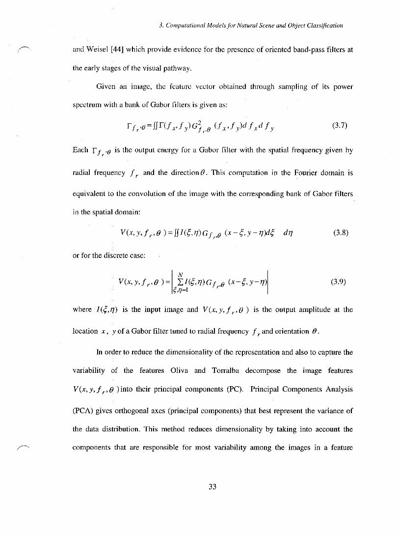
3. Computational Modelsfor Natural Scene and Object Classification
and Wei sel [44] which provide evidence for the presence of oriented band-pass filters at
the early stages of the visual pathway.
Given an image, the feature vector obtained through sampling of its power
spectrum with a bank of Gabor filters is given as:
(3.7)
Each r f r,f) is the output energy for a Gabor filter with the spatial frequency given by
radial frequency f r and the direction e. This computation in the Fourier domain is
equivalent to the convolution of the image with the corresponding bank of Gabor filters
in the spatial domain:
or for the discrete case:
N V(x,y,fr,e)= IJ(;,17)Gf
r,f) (x-;,y-TJ)
;,1]=1
(3.8)
(3.9)
where 1(;,17) is the input image and V(x, y, f r' e) is the output amplitude at the
location x, y of a Gabor filter tuned to radial frequency f r and orientation e.
In order to reduce the dimensionality of the representation and also to capture the
variability of the features Oliva and Torralba decompose the image features
V(x,y,fr,e )into their principal components (PC). Principal Components Analysis
(PCA) gives orthogonal axes (principal components) that best represent the variance of
the data distribution. This method reduces dimensionality by taking into account the
components that are responsible for most variability among the images in a feature
33

3. Computational Models lor Natural Scene and Object Classification
space. To thls purpose covariance matrices are formed for each f rand e using feature
vectors V(x,y,fr,e )obtained from aIl training images in the database. The
decomposition of the covariance matrices produces the eigenvectors lf/ n (x, y, f r' e ).
The coefficients al r,(},d are produced by the projection of the image features
v (x, y, f r' e ) onto the principal components lf/ d (x, y, f r' e ).
D
V(x,y,fr,e)= Lafr,B ,dlf/d(x,y,fr,e) d=l
(3.10)
The coefficients {al r'(} ,n} for the radial frequencies f r and orientations e and the
principal components d = L.D are used as an estimation of the context features of the
images. The dimensionality of the context features depend on the choice of the number
of filters in the Gabor set and the choice of D. We will discuss the effect of choice of D
in our model further in chapter 5. The coefficients {al r'(} ,d} incorporate information
about the spectral characteristics of the images and their spatial arrangements. The
ability of this representation for scene categorization task and its ability to account for
attributes meaningful to observers has been investigated and demonstrated in Oliva and
Torralba [37].
3.1.3 Proposed Scene Module Formulation
We choose the feature vector Vc={alr,(} ,dl as the scene representation for our model,
and we caU V c the global image feature. Assuming m scene classes Sb S 2"'" Sm' and
global context features V c of an input image given to the scene module, the probability
34
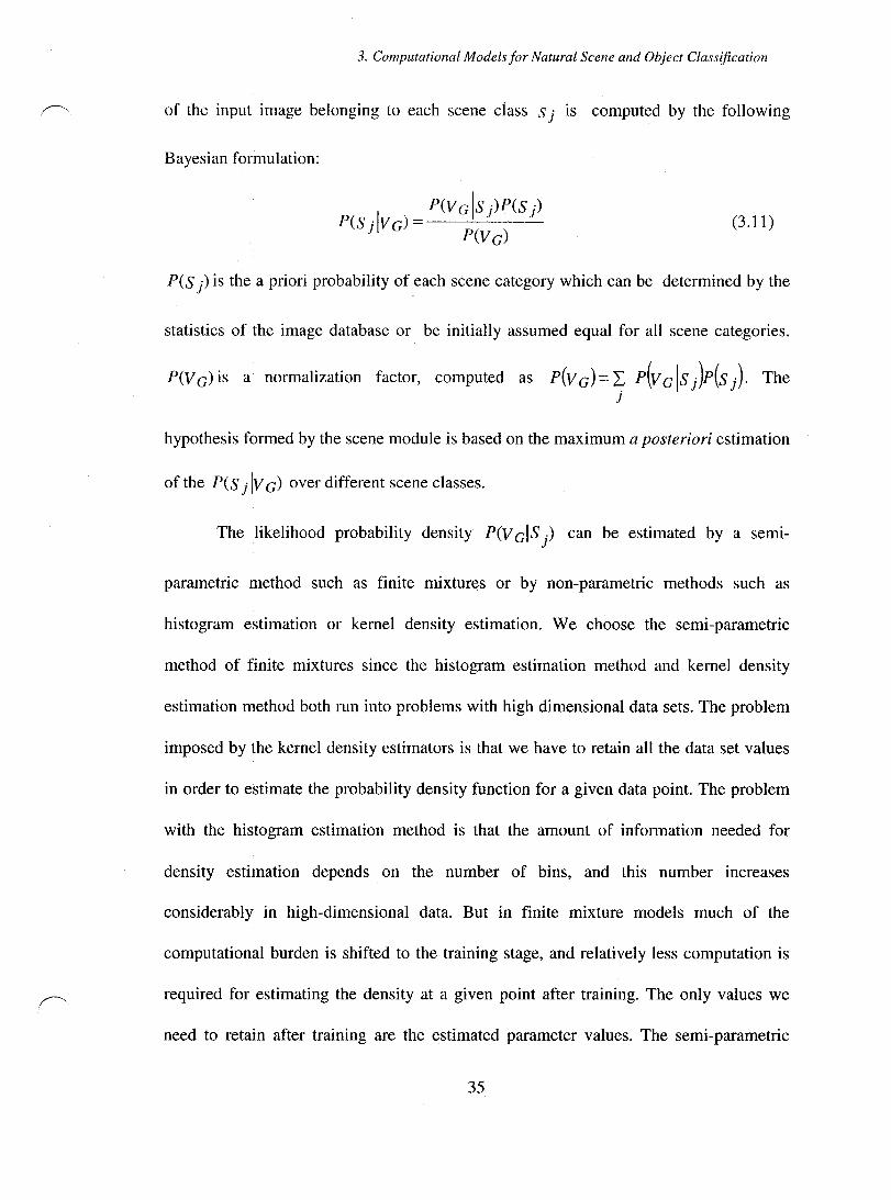
3. Computational Models for Natural Scene and Object Classification
of the input image belonging to each scene ciass S j IS computed by the following
Bayesian formulation:
1
PCV c Is )P(S j) P(S j V c) = --P--'-(-V-c)-- (3.11 )
P(S j) is the a priori probability of each scene category which can be determined by the
statistics of the image database or be initially assumed equal for all scene categories.
pcv c) is a normalization factor, computed as p(V c) = ~ p{v c Is Jp{s j). The }
hypothesis formed by the scene module is based on the maximum a posteriori estimation
of the P(S j Iv c) over different scene classes.
The likelihood probability density PcV clS) can be estimated by a semi-
parametric method su ch as finite mixtures or by non-parametric methods such as
histogram estimation or kemel density estimation. We choose the semi-parametric
method of finite mixtures since the histogram estimation method and kemel density
estimation method both run into problems with high dimensional data sets. The problem
imposed by the kemel density estimators is that we have to retain aIl the data set values
in order to estimate the probability density function for a given data point. The problem
with the histogram estimation method is that the amount of information needed for
density estimation depends on the number of bins, and this number increases
considerably in high-dimensional data. But in finite mixture models mu ch of the
computational burden is shifted to the training stage, and relatively less computation is
required for estimating the density at a given point after training. The only values we
need to retain after training are the estimated parameter values. The semi-parametric
35
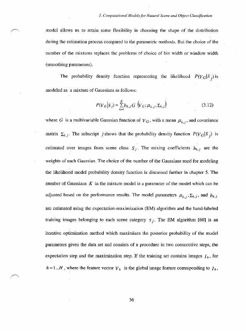
3. Computational Modelsfor Natural Scene and Object Classification
model allows us to retain sorne flexibility in choosing the shape of the distribution
during the estimation process compared to the parametric methods. But the choice of the
number of the mixtures replaces the problems of choice of bin width or window width
(smoothing parameters).
The probability density function representing the likelihood PCV GIS) is
modeled as a mixture of Gaussians as follows:
(3.12)
where G is a multivariable Gaussian function of V G' with a mean flk ., and covariance ,j
matrix Lk,j' The subscript j shows that the probability density function PCV GIS) is
estimated over images from scene class S j' The mixing coefficients bk,j are the
weights of each Gaussian. The choice of the number of the Gaussians used for modeling
the likelihood model probability density function is discussed further in chapter 5. The
number of Gaussians K in the mixture model is a parameter of the model which can be
adjusted based on the performance results. The model parameters flk,j' Lk,j' and bk,j
are estimated using the expectation-maximization (EM) algorithm and the hand-labeled
training images belonging to each scene category S j' The EM algorithm [60] is an
iterative optimization method which maximizes the posterior probability of the model
parameters given the data set and consists of a procedure in two consecutive steps, the
expectation step and the maximization step. If the training set contains images 1 h, for
h = 1 ... H , where the feature vector V h is the global image feature corresponding to 1 h ,
36
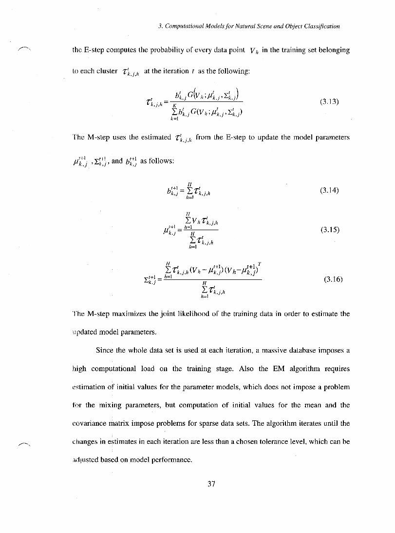
3. Computational Modelsfor Natural Scene and Object Classification
the E-step computes the probability of every data point V h in the training set belonging
to each cluster rLj,h at the iteration t as the following:
(3.13)
The M-step uses the estimated r~,j,h from the E-step to update the model parameters
Hl H' d t+l + Il f.1k,j , Lk,j' an bk,j as 10 ows:
H
bt+l _ ",.,.1 k'-~"k'h ,J h=l ,J,
H
IVhrL,h f.1t+1 _ .:..;..h=--=l __ _
k,j- H
IrL,h h=1
(3.14)
(3.15)
(3.16)
The M-step maximizes the joint likelihood of the training data in order to estimate the
Il pdated model parameters.
Since the whole data set is used at each iteration, a massive database imposes a
high computational load on the training stage. Also the EM algorithm requires
estimation of initial values for the parameter models, which does not impose a problem
for the mixing parameters, but computation of initial values for the mean and the
covariance matrix impose problems for sparse data sets. The algorithm iterates until the
changes in estimates in each iteration are less than a chosen tolerance level, which can be
adjusted based on model performance.
37

3. Computational Models for Natural Scene and Object Classification
3.2 Computational Model for Object Classification
Replicating the human ability to recognize different object categories is one of the most
difficult challenges which face computational vision scientists in this decade. Humans
are able to recognize more than 104 categories of objects by the time they are six years
o]d, and keep learning more through life [8]. The literature on the topie of object
presentation and object recognition is very rich, but one can generalize the various
approaches to three general dichotomies. The early approach to object presentation was
to con si der an object as made up of a distinctive collection of features, and to attempt to
achieve recognition through detection of features and their combinations. MaIT [59] and
Biederman [8] proposed a different view of the vision process, in whieh a 2-dimensional
retinal image is first transformed to a 3-dimensional representation, whieh forms a basis
for recognition. Based on this view, Biederman proposed an elaborate theory for object
recognition, where objects are represented as collection of geometric ieons (geons),
which are 3-dimensional shapes that produce viewpoint invariant 2-dimensional
projections. An alternative "appearance-based" view of object representation was
proposed by Poggio and Edelman [75] and TaIT and Bulthoff [92] that suggests objects
are recognized on the basis of a small number of stored 2-dimensional views. The main
challenge of aIl three approaches is that in order to capture the great diversity of forms
and appearances of objects, the models must contain hundreds, and sometimes thousands
of parameters. Estimation of these parameters in volves batch training with large sets of
examples. Compounding this diffieulty are other factors su ch as occlusion, clutter,
lighting and shading, view points, scales, all of whieh make recognition harder. Recent
work has highlighted the ability of humans to learn object categories from small number
38

3. Computational Modelsfor Natural Scene and Object Classification
of examples and in an incremental manner (as opposed to the large training sets and
batch learning common in computational vision methods) and have attempted to
replicate these abilities into computational vision a1gorithms [24][22][25].
In view of the complications of an elaborate model for object· category
representation, we searched for a relatively simple method which would be adequate for
our experimental setup of discrimination among a few chosen set of object classes. Sorne
recent work on object classification focuses on special interest categories: human faces
[53] [82][89][84][103], pedestrians [104], hand written digits [52], and automobiles [84]
[26]. Instead we need a method that would apply well to a variety of different object
categories. Researchers who have addressed the prob1em of multi-category recognition
[26][106][12] choose rich representation models with many parameters for object
categories in order to be able to capture the diversity of different category appearances.
They do not deal with variability in view-point and lighting and occlusion explicitly, but
as additional factors for intra-class variability, therefore there is no requirement for
alignment of objects, lighting normalization, or segmentation of the images as a
preprocessing stage.
We define our problem as recognizing one object category out of a number of
possible object categories, from image patches which have been extracted from a natural
scene image. Our goal is to extract sorne local information about the probabilities of
having different object categories in that location of image. Image patches are extracted
from a tessellation of the scene image in different scales, so a patch may be dominated
by one object or part of an object, or be a cluttered part of the scene with no dominant
object, or belong to the background. There is generally a lot of clutter and occlusion
39

.~.
3. Computational Models for Natural Scene and Object Classification
present in the "images and few patches in a scene may contain a dominant un-occluded
object. The objects appear in a variety of sc ales and from different view points which are
only constrained by the scene context (certain view points of objects, or certain scales of
objects, are very improbable in certain scene contexts).
In choosing a model for representing different object categories we rely on
experimental results presented by Oliva and Torralba [95]. In order to study the effect of
scale in their proposed method for scene representation, they have also experimented
with close-up images (or cropped sections of images) which contain mainly one object
category. Their results show that the sorne object categories can be characterized by their
me an power spectra. For example fig 3.2 shows characteristic spectra for man made
objects versus natural objects. Motivated by this result we have investigated the
possibility of categorizing image patches containing our chosen set of object classes
(vehicles, buildings, furniture, people, and plants) using spectrum-based features. We
created a set of image patches in different scales, by cropping the scene images in our
data base by hand and selecting patches which bound one whole object. We did not
impose a limitation on objects view points or orientations, but these factors are highly
constrained by the scene context. Our experiments indicate that we can use the features
extracted by sampling the mean power spectra, as explained in detail in section 3.1.2, for
a reliable classification of object-patches, within this chosen set of object categories. We
would like to emphasize that we do not daim that this method can serve as a successful
object category model in general. The object categories we have chosen differ in texture,
dominant orientation of structural components, and smoothness of surfaces, which may
count for the success of this modeling for our purposes. The utility of this model may
40

~ ..
3. Computational Models for Natural Seene and Object Classification
break however, with a different choice of object categories. The PCA stage in feature
extraction maximizes the variability of the selected features among the chosen classes.
We choose a probabilistic framework for classification in these experiments, and the
statistical modeling of the object category features allows us to de al with the problems of
variations in view point, occlusion, background clutter, and lighting implicitly as intra
category variability. We de al with the problem of scale more explicitly in the model
which is discussed in detail in the following section.
3.2.1 Proposed Object Module Formulation
Given an input image to the model, the object module estimates the probability of
presence of objects from different object categories in local regions of the image (image
patches). The object module processes local information while the scene module
processes global scene information. Local regions of an image may be extracted using
different methods. We choose a sliding rectangular window for extracting patches from
the image, where the center of the sliding window moves on an evenly sampled grid in
order to provide a uniform covering of the image. Patches of different sizes are used for
extracting regions of different scales in the image. Each sc ale is denoted by Tl, with
1 = 30,50,70,90,110 pixels, corresponding to patches with height of 30, 50, etc. pixels.
For each extracted patch the feature vector VL={afr,8 ,d} is computed using the Oliva
and Torralba method described in section 3.1.2.
The probability of a patch of scale Tl representing an object belonging to one of
the n different object classes OI>02, ... ,On is given by:
41
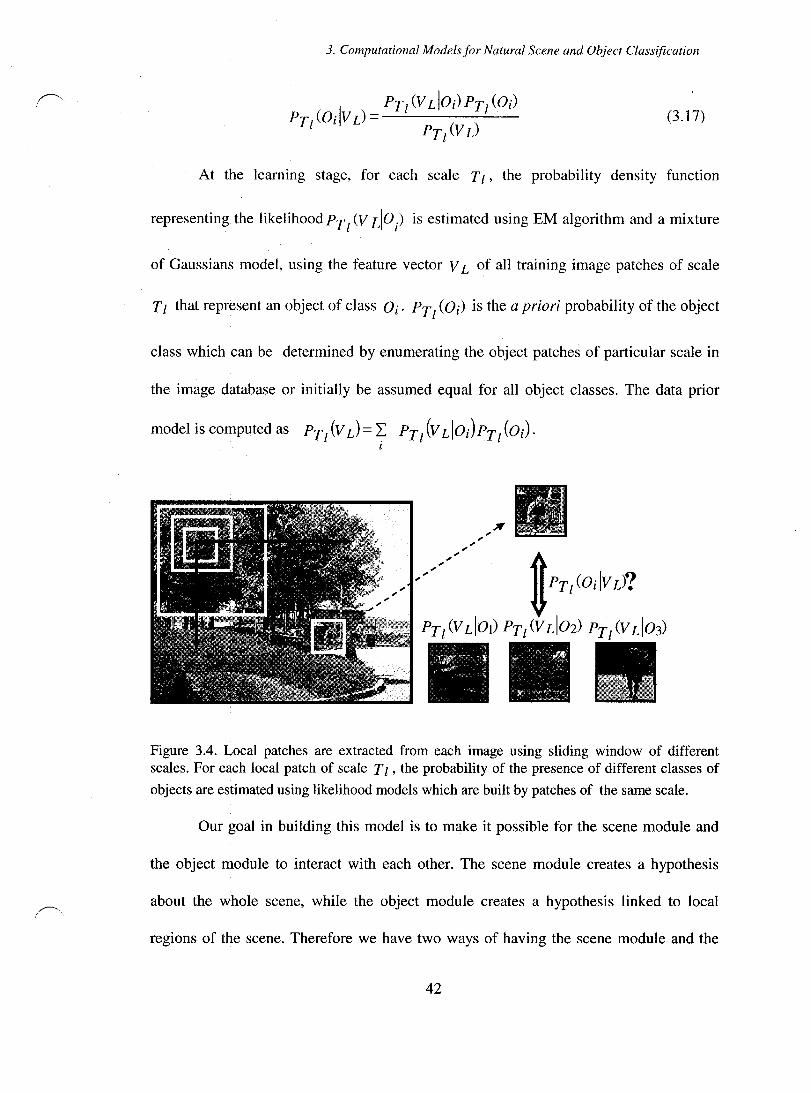
3. Computational Modelsfor Natural Scene and Object Classification
(3.17)
At the learning stage, for each scale Tl, the probability density function
representing the likelihoodPT/V LlO) is estimated using EM algorithm and a mixture
of Gaussians model, using the feature vector V L of all training image patches of scale
Tl that represent an object of class Oi' PTz (Oi) is the a priori probability of the object
class which can be determined by enumerating the object patches of particular scale in
the image database or initially be assumed equal for all object classes. The data prior
model is computed as PT z (V L) = I; PT /V L loJ PT z (oJ 1
Figure 3.4. Local patches are extracted from each image using sliding window of different scales. For each local patch of scale T z , the probability of the presence of different classes of
objects are estimated using likelihood models which are built by patches of the same scale.
Our goal in building this model is to make it possible for the scene module and
the object module to interact with each other. The scene module creates a hypothesis
about the whole scene, while the object module creates a hypothesis linked to local
regions of the scene. Therefore we have two ways of having the scene module and the
42

3. Computational Modelsfor Natural Seene and Object Classification
object module interact. We can either let each local region propagate the results of its
local processing to the scene module independently, and then average or aggregate the
results of the independent interactions of each local region with the whole scene, at the
scene level. Or we can combine the results of local processing of the regions produced
by the object module before any interaction with the scene module and then adjust the
scene module according to the combination of the object module results. This issue is
actually the crux of the model and one of the most important problems to resolve. In
order to address this issue we have to decide what kind of information we want to
transfer between the two modules. There are three types of information produced by the
object module, the identity of the objects, the scales, and the locations of the objects. The
scene module can make use of aIl these three types of information to adjust its estimate
of the scene type, although they may not be necessary. In the present implementation of
the model, we focus on the identity of the objects. We would want to pass the
information extracted by the object module about the possible object categories present
III the image to the scene module but not specifie information about their locations or
scales. In this case there is no need for local region processes interacting individually
with the scene module. Therefore we integrate the local hypotheses represented by the
posterior PT/odv L) from different patch locations and different scales into one
hypothesis which we represent by P(Oi 1 { V L} ). One can think of averaging aIl the
probability distributions PTI (0 Iv Ü over all the patches of different scales and
different locations. But a simple averaging of the probability distributions would run into
43

3. Computational Modelsior Natural Scene and Object Classification
several issues. We propose a weighted average of the distributions using the following
technique:
1. A weighted average is computed where the posterior probability distributions
which present low certainty decisions (based on the preset decision thresholds)
are assigned a lower weight compared to posterior probability distributions which
present high certainty decisions. (We do not want a lot of regions with posteriors
representing uncertain decisions cancel out the effect of regions with certain
decisions ).
2. The distributions are weighted according to their scale, with a higher weight for
distributions belonging to larger scale reglOns and a smaller weight for
distributions belonging to smaller scale reglOns. Certainty or uncertainty of
decision for larger scale regions has more effect on the weighted average
compared to certainty or uncertainty of decision for sm aller sc ale regions. The
adverse effect of this weighting is that the effects of many small instances of an
object have to aggregate to have the effect of one instance of object in a larger
scale, which may not be always meaningful.
In order to resolve the issue of over-counting evidence we take the following
measures:
1. We start computing the local estimation with the patches of highest scale, and at
each scale level we discard aIl the smaller scale patches falling inside a higher
scale patch with a high certainty decision. We also avoid over-counting evidence
for objects which are self-similar in different scales (e.g. plants).
44

3. Computational Modelsfor Natural Scene and Object Classification
2. We discard regions with small likelihood values, reglons which the
measurements do not give evidence that one of the known object categories is
present, regions with unknown objects, or background dutter. In such a case the
Bayesian formulation copies the prior model to the posterior. In the future design
of the model this issue will cause a problem because we count evidence for
wrong regions.
3. In order to avoid over-counting evidence from overlapping regions we compare
the change in the posterior estimation for regions in a neighborhood and if the
changes in probability values are smaller than a threshold, we discard the
overlapping patch.
The global probability distribution P(O 1 { V L}) is thus created as a weighted
average over the local posterior probability distributions, with the probability
P(Oi 1 { V L}) containing information about the frequency of presence of object category
Oi across all scales and across aIl locations in the scene.
3.3. Summary
We use the scene representation introduced by Oliva and Torralba, based on the
sampling of the mean power spectrum of images with Gabor filters of different scales
and orientations, for scene categorization. We also use a similar representation for
extracting features from local image regions for object categorization. Figure (3.5)
presents a general schema of the model discussed in this chapter. The function of the
scene and the object modules are formulated using Bayesian inference processes. In the
45
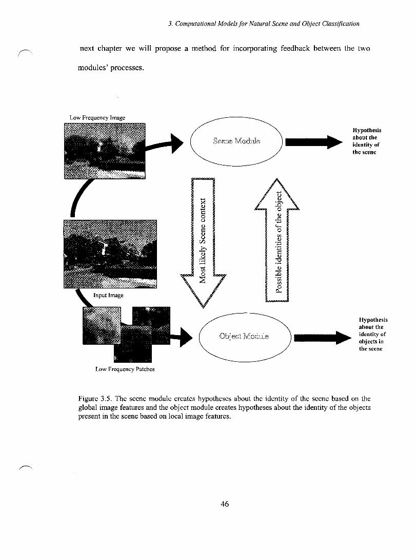
3. Computational Models for Natural Seene and Object Classification
next chapter we will propose a method for incorporating feedback between the two
modules' processes.
Low Frequency Image
CI)
~ 0 <)
CI)
~ CI) <)
rfJ ~ -CI)
~ ..... -
Low Frequency Patches
CI)
-5 4-< 0 <:Il CI) ..... ...... ..... ~ CI)
"0 . .... CI) -..0 .....
Hypothesis about the identity of the scene
Hypothesis about the identityof objects in the scene
Figure 3.5. The scene module creates hypotheses about the identity of the scene based on the global image features and the object module creates hypotheses about the identity of the objects present in the scene based on local image features.
46
4. Coupling of the Scene Classification Module and the Object Classification Module
Chapter 4
Coupling of the Scene Classification Module and the Object Classification Module
In this chapter we present the mathematical methodology we have developed through
which the information produced by the two sensory information processing modules, the
scene classification module and the object classification module, can become available
to each other and be considered as part of the information processing problem solved in
each module. The methodology we present here is motivated by the field of data fusion,
which is concemed with the methods of combining various information sources. In
section 4.1 we motivate our proposed methodology in the framework of Bayesian data
fusion. In section 4.2 we distinguish between two classes of data fusion
implementations, the weak coupling and the strong coupling architectures. In section 4.3
we propose two approaches for implementing the interactions between the scene
classification and the object classification modules based on a Bayesian strongly coupled
data fusion architecture.
4.1 Data Fusion
Data fusion deals with the question of fusing separate sensory information processing
components in order to achieve a globally "better" solution to the sensory information
processing problem at hand, as compared to the solutions given by each of the individual
components. The global system improves the performance of the task at hand by
producing a solution which is more accurate than the components' solutions or by
47

4. Coupling of the Scene Classification Module and the Object Classification Module
producing a unique solution when the individual components are not able to produce any
unique solutions individually. The latter aspect of data fusion algorithms have been
described by Clark and Yuille [14] in terms ofregularization ofill-posed problems.
Clark and Yuille view the problem of image understanding or "perception" as a
process of inverting the world-to-sensed-data mapping. Since the sensing process
pro duces a non-invertible projection of the world (i.e. the mapping from the world
structures to the image space is many to one), in order to invert this mapping one must
constrain the set of possible world interpretations of the sensed-data to a degree where
the mapping from the reduced space to the image space becomes invertible. In other
words sensing involves a non-invertible projection of the world which makes perception
(sensory information processing task) an ill-posed problem; therefore in order to
regularize such an ill-posed problem, and for a sensory processing module to operate
adequate1y (being able to pro duce unique solutions to the task at hand), constraints of
one form or another must be imposed on the solution process. These constraints can be
"physical constraints", "natural constrains", or "artificial constraints". Physical
constraints are based on rules of physics and mathematics and rule out solutions which
are physically impossible. Natural constraints are derived from observations from the
environment and represent conditions which are normally and naturally true in that
domain (examples of natural constraints used in computer vision problems are surface
smoothness, object rigidity, Lambertian surface reflectance). Artificial constraints embed
expectations about the state of the world based on high leve1 knowledge of the domain,
formed from previous estimates of the state of the world. Physical constraints are
universally valid, but natural and artificial constraints are not. Furthermore, it is
48

4. Coupling of the Scene Classification Module and the Object Classification Module
sometimes not possible to find natural and artificial constraints which are always valid,
even within the specifie domain of the problem. In cases where the constraints imposed
on the information processing module are not valid, or are insufficient, the module may
produce a wrong solution or be unable to find a unique solution to the problem.
One way to address this problem is to use the information produced by another
information processing unit to correct the answer of the module. In this way combining
or fusing results obtained from several modules enhances the performance of the system
as a whole. So fusion of information produced by different components of a sensory
system can reduce the dependency of the solution of the system on invalid or insufficient
constraints imposed on the solution process within each module. In this sense, data
fusion can be seen as a method of regularizing the ill-posed problem of perception (or
any other ill-posed problem for that matter) not only by means of a priori constraints
(constraints not based on CUITent sensory data), but also by constraining it by information
which cornes from a "partial" solution to the problem and is obtained from independent
sensory information processing modules (based on the current sensory data).
In the Bayesian approach to solving sensory information processing problems,
different possible solutions are assigned a probability based on the models of the sensing
process (likelihood model) and models representing general assumptions made about the
world (a priori models). One of the advantages of the Bayesian formulation is that it
provides a suitable form for embedding constraints into the solution process. Sorne of
the constraints required for the solution process are incorporated and embedded into the
likelihood models when these models are being estimated using sensory measurements.
One can also choose the a priori models to enforce the necessary constraints on the
49
4. Coupling of the Scene Classification Module and the Object Classification Module
solution process. Usually the a priori models incorporate constraints which are based on
general assumptions made about the domain (before any measurements are made), but
the priors can also be influenced by the previous measurements (as in the case of active
vision). The likelihood models typically involve physical, and to a lesser extent natural
constraints, while the prior models typically involve natural and artificial constraints
[14].
In the Bayesian approach that we have chosen for determining the semantic
context of a scene and for determining the presence or absence of certain object classes
in the scene, scene and object classification are formulated as estimating the following a
posteriori conditional probabilities:
1
P(V GIS)p(S) P(S . V G) = ------'----
J P(V G) (4.1)
(4.2)
The conditional probabilities P(V Gis j) and PT, (V LI Qi) represent probabilities of
occurrence for the input measurement data on the event that it is known that the
measurements belong to scene class S j or object class Qi respectively. The likelihood
P(V Gis j) represents the mapping from the class of scenes S j to the space of image
features V Gand similarly PTt (V L 1 Qi) represents the mapping from the class of objects
Oi to the image features V L' Universally valid physical constraints and certain domain
specific natural constraints (e.g. certain structural rules normally valid for most
50

4. Coupling of the Seene Classification Module and the Object Classification Module
contextually meaningful scenes such as sky above earth, horizontal layers along
dominant horizon) are embedded into these conditional probabilities during the learning
stage through the training patterns.
On the other hand the a priori models P(S j) and PT, (Oi) constrain the solution
with general assumptions made about the scene classes Sj and object classes Oi' In the
previous chapter we mentioned that the a priori models P(S j) and PT, (Oi) are
computed using the statistics of the database to represent how likely a given scene or
object is, before any measurements are made. But it is not al ways possible to estimate an
informative a priori model for the problem this way (for example a training database
where aIl the scene and object classes have equal probability of presence will produce a
uniform a priori model for the problem). In cases where the a priori models are
uninformative, the solutions to equations (4.1) and (4.2) are reduced to a maximum
likelihood estimation of the two equations.
In cases where the constraints embedded in the likelihood models or a priori
models are not valid or are insufficient, the scene classification module or the object
daqsification module may produce a wrong solution or be unable to find a unique
solution to the problem. In such a case one can supplement the a priori constraints
(constraints not based directly on the measurements from the sensory data) with extra
constraining information obtained from the other information processing module. For
example in the problem of scene classification of a given image, if the object module has
independently determined with a high reliability that certain objects exist in the image,
but the scene module is not able to classify the image reliably, then the knowledge about
51

4. Coupling of the Scene Classification Module and the Object Classification Module
the objects present in the scene can be used for further constraining the scene module
solution process. For example knowledge of the relationships between scene categories
S j and object categories ai, in the form of conditionals ail S j and S j lai can be used to
develop a more informative a priori model for the scene module. It is this Bayesian view
of data fusion which forms the theoretical basis for our proposed method of
implementing informative interactions between the scene and the object modules.
Based on the Bayesian interpretation of data fusion, information from
independent information processing modules can be used to impose constraints on either
the likelihood models or the prior models of a Bayesian estimation process. The
alteration of either the likelihood models or the prior models, in order to accommodate
information coming from an independent source, is the basis for distinguishing between
two methods of coupling the object and the scene modules, as proposed later in this
chapter. Before describing our proposed method for "constraint embedding" or "data
fusion" between the scene classification and the object classification modules, it is
necessary to distinguish between weakly versus strongly coupled data fusion
architectures.
4.2 Weakly and Strongly Coupled Architectures for Data Fusion
The research performed on data fusion systems has been carried out largely within the
engineering community [15][102][105] and overlaps substantially with the work on
multiple classifier systems in the area of pattern recognition. In this body of work
different architectures (for example seriaI, parallel, hierarchical) have been considered
for implementing data fusion, but often the adopted architectures are developed in an ad
52

4. Coupling of the Scene Classification Module and the Object Classification Module
hoc manner dictated by the practical application at hand. Two major classes of fusional
architectures have been distinguished by Clark and Yuille [14]; that of weakly coupled
and strongly coupled data fusion. These two classes differ in the way the constraints
(information from other sensory modules) are embedded into the solution processes.
In the weakly coupled data fusion model the outputs of several sensory
information processing modules are combined in a fusion module to produce a global
system solution for the desired task. The general architecture for a weakly coupled data
fusion system is presented in figure (4.1). As illustrated in figure (4.1) the modules Ml,
M 2 , ... , ML process the feature space, and the information processing function
performed by the modules are independent from each other. In the weakly coupled
architectures the supplementary constraints required for the solution process are imposed
through the fusion module. From a Bayesian point of view the likelihood models and the
a priori models of different modules do not depend on the output of any other module,
and the solution process of the component modules are not altered to accommodate extra
constraints from other sources.
The information fusion models studied in the area of pattern recognition under
the title of "classifier fusion models" are weakly coupled architectures. Examples of
these models are the classifier combiners based on Bayesian decision mIes proposed by
Kittler et al [49], classifier combiners based on class predictions proposed by Lam and
Suen [51] and Huang and Suen [43], combiners based on stack generalization, mixture
of expert models proposed by Jacobs et al [47] and Jordan and Jacobs [48], bagging
[10], boosting methods proposed by Freund and Schapire [28] [29], and dynamic
classifier selection method proposed by Woods et al [109]. These models deal with the
53
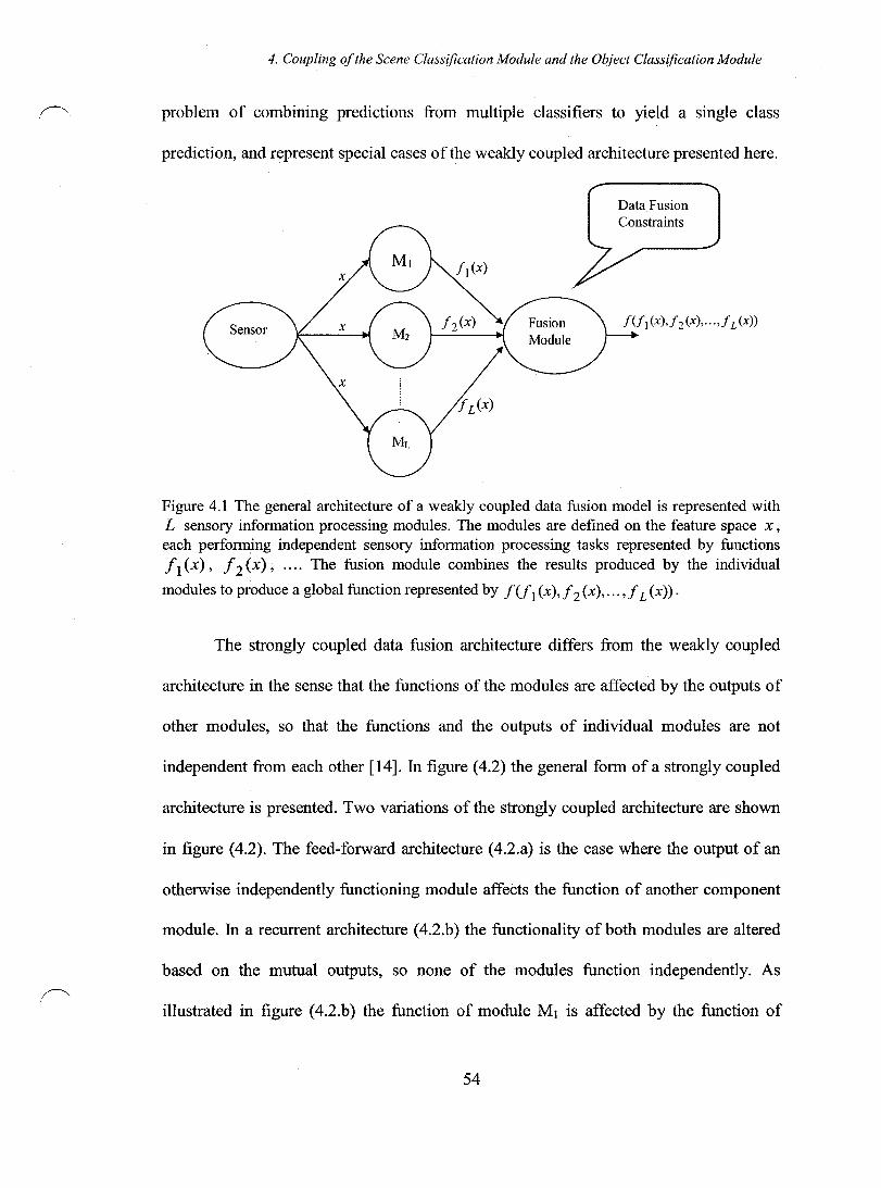
4. Coupling of the Scene Classification Module and the Object Classification Module
problem of combining predictions from multiple classifiers to yield a single class
prediction, and represent special cases of the weakly coupled architecture presented here.
Data Fusion Constraints
Figure 4.1 The general architecture of a weakly coupled data fusion model is represented with L sensory information processing modules. The modules are defined on the feature space x, each performing independent sensory information processing tasks represented by functions Il (x), 12 (x), .... The fusion module combines the results produced by the individual
modules to produce a global function represented by f (f 1 (x), f 2 (x), ... ,f L (x» .
The strongly coupled data fusion architecture differs from the weakly coupled
architecture in the sense that the functions of the modules are affected by the outputs of
other modules, so that the functions and the outputs of individual modules are not
independent from each other [14]. In figure (4.2) the general forrn of a strongly coupled
architecture is presented. Two variations of the strongly coupled architecture are shown
in figure (4.2). The feed-forward architecture (4.2.a) is the case where the output of an
otherwise independently functioning module affects the function of another component
module. In a recurrent architecture (4.2.b) the functionality ofboth modules are altered
based on the mutual outputs, so none of the modules function independently. As
illustrated in figure (4.2.b) the function of module Ml is affected by the function of
54
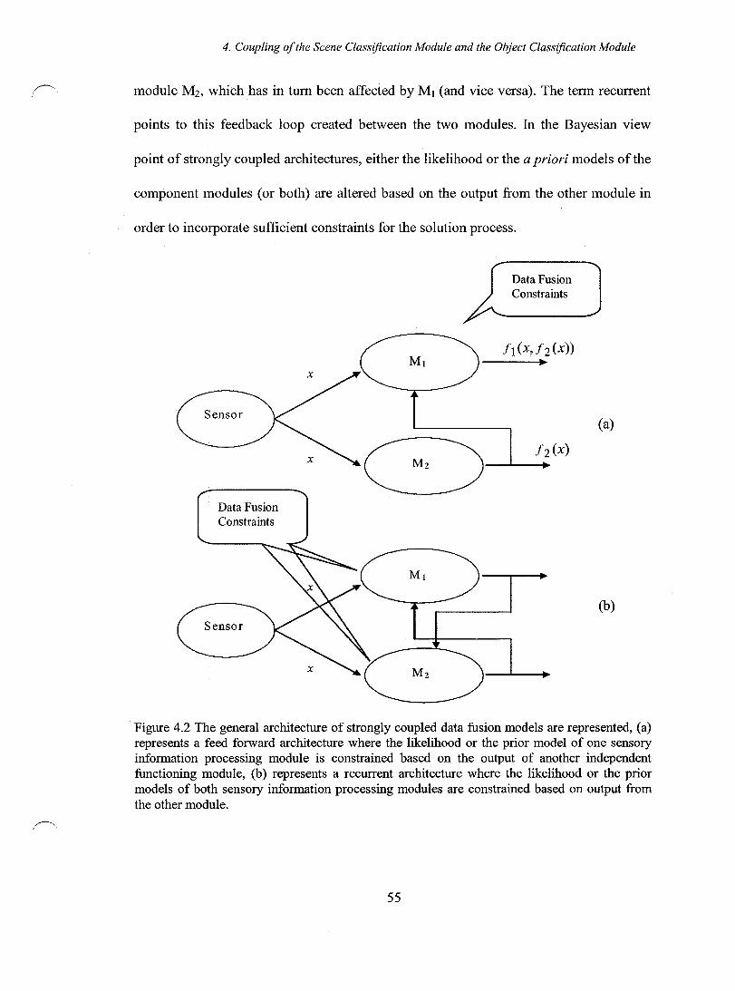
4. Coupling of the Scene Classification Module and the Object Classification Module
module M2, which has in tum been affected by Ml (and vice versa). The terrn recurrent
points to this feedback loop created between the two modules. In the Bayesian view
point of strongly coupled architectures, either the likelihood or the a priori models of the
component modules (or both) are altered based on the output from the other module in
order to incorporate sufficient constraints for the solution process.
Data Fusion Constraints
Sensor
M2
Data Fusion Constraints
fI (x, f 2 (x)) ~
(a)
(b)
Figure 4.2 The general architecture of strongly coupled data fusion models are represented, (a) represents a feed forward architecture where the likelihood or the prior model of one sensory information processing module is constrained based on the output of another independent functioning module, (b) represents a recurrent architecture where the likelihood or the prior models of both sensory information processing modules are constrained based on output from the other module.
55
4. Coupling of the Scene Classification Module and the Object Classification Module
An example of strongly coupled data fusion architecture in literature is the
Kalman filtering method [32]. The Kalman filter estimates a variable which represents a
sequence of changing states of the world, and involves recursively updating the a priori
model of the state variable based on previous and currentestimates of the state variables
and updating the estimate of the state variable based on the current a priori model, the
system model, and the measured data. The Kalman filter is a strongly coupled model in
the sense that the a priori model is adapted in a data dependant way.
A general characterization of the function of a module III the Bayesian
implementation of a strongly coupled data fusion model is given by Clark and Yuille
[14] as foUows:
p(x Iv ; ZJ, Z2, ... , Zn)P(V ; ZJ, Z2, ... , Zn) pCv 1 x) = -----------
p(x ; Zb Z2, ... , Zn)
(4.3)
where the function of the module is to determine a parameter v by optimizing the
conditional density pCv 1 x), where x is the measured data input to the Bayesian
parameter estimation module, and Zl, Z2, ... , Zn are the data from the other sensory
information producing modules. The likelihood model, the a priori model, and the data
model aU can be seen as functions of Zl, Z2, ... , Zn . The output Zk of a given module which
influences the estimation process of parameter v, can itself in tum be influenced by the
function of this module. This formulation includes the adaptation of both the a priori
model and the likelihood models.
56

4. Coupling of the Scene Classification Module and the Object Classification Module
4.3 Strongly Coupled Data Fusion between Scene and Object Modules
In the previous section we mentioned that in cases where the a priori constraints built
into the scene classification module and the object classification module fail to provide a
unique solution for one of the modules, the knowledge inferred from the other module
can be combined as part of the module estimation process in order to further constrain
the solution. We are motivated by the strongly coupled data fusion architecture
illustrated in figure (4.2) and the general formulation in equation (4.3) to modify our
Bayesian solutions for the scene and the object classification modules in order to
incorporate possibility of information sharing between the two modules. As discussed in
the previous section the strongly coupled data fusion architecture allows two approaches
to implementing the interactions between the two modules. In the first approach, the two
modules interact through the prior terms of the Bayesian formulation. In this approach
the a priori models of the scene and object modules are modified in order to allow
constraints built into the solution process based on information coming from the other
module. This variation of the model is strongly coupled in terms of priors. In the second
approach, the likelihood models of each module are reformulated in order to allow data
fusion with the other module. This variation of the model is strongly coupled in terms of
likelihoods. For both variations of the model we present are examples of recurrent
strongly coupled architecture.
4.3.1 Adaptive Priors Model
The key idea in this approach is that the any previously acquired knowledge about the
scene identity affects the a priori models used for the object identification process, and
likewise any previously acquired knowledge about the objects present in the scene
57

4. Coupling of the Scene Classification Module and the Object Classification Module
affects the a priori models used for the scene identification process. In our proposed
model we revise the Bayesian estimation equations (4.1) and (4.2) in order to embed a
feedback interaction between the two modules. In order to make feedback connections
possible between the two modules, the a priori terms in equations (4.1) and (4.2) are
expanded as following:
P(S) = IP(Sj,Oi) = IP(SjloJP(oJ i i
(4.4)
PT/ (Di) = ~ PT/ (Di' S) = ~ PT/ (Oil S j)P(S j) (4.5) J J
Expanding the a priori terms as In equations (4.4) and (4.5) exploits the
dependency of the scene level priors and the object leve1 priors to provide a way to feed
back the output of the one module to the other module. Equation (4.4) shows how the a
priori term P(S) can be modified based on knowledge of the probability of the
presence of different object classes in the scene. Ifthere is no previous knowledge of the
different object classes present in the scene, the a priori term P(S j) of equation (4.1)
can be determined based on the statistics of the database or be assumed equal for aIl
scene classes (as done for the first iteration of the model), but once the object module
has made inferences about the probability of the presence of different object classes in
the scene, this knowledge can be used to provide a new estimation of the a priori term
P(S) based on equation (4.4), where the term P(O,) in equation (4.4) is updated based
on the new a posteriori distributionP(Oi 1 {V r}) produced by the object module.
Similarly equation (4.5) shows how the knowledge acquired by the scene module about
the probability of the image belonging to different scene classes can affect the a priori
probability of the presence of different objects in the scene. The new estimation of the
58

4. Coupling of the Scene Classification Module and the Object Classification Module
prior term PTt (Oi) is estimated by updating the terms P(S) in equation (4.5) based on
the new a posteriori P(S j Iv G) produced by the scene module.
The data dependent alteration of the a priori terms distinguishes this model as a
strongly coupled architecture. The mutual feedback between the two modules
characterizes the model as a recurrent feedback system. At the first iteration of the model
the scene and object modules perform their Bayesian estimation process independently
and without any feedback from the other module; therefore, the result of first iteration
shows how well the modules can function on their own and if there is any need for
information sharing between the modules. If there is no reliable estimate made by either
of the two modules then the feedback connections are activated, and new estimates of
scene and object classes are made through the recurrent feedback between the two
modules.
The feedback is designed to use the new information inferred by the system at
each iteration, to determine a more accurate a priori model for the specific scene class.
The a priori models representing different scene classes in the Bayesian equation (4.1)
are not the same if there is any previously acquired knowledge of the type of objects
found in the scene. Aiso the a priori models representing different object classes in the
Bayesian equation (4.2) are not the same if there is any previously acquired knowledge
of the image scene type. Expanding the a priori models P(S) andPT/OJ as in
equations (4.4) and (4.5) allows the readjustment of the weights of the conditional
probabilities P(S jl Oi) and PTt (Oil S) in order to incorporate the effect of the
knowledge acquired by the other module.
59
4. Coupling of the Scene Classification Module and the Object Classification Module
It is important to show that the modification of the priors given in equations (4.4)
and (4.5) produces valid a priori probability distributions. In order to have valid a priori
and a posteriori probability distributions in equations (4.1) and (4.2), we have to show
that LP(S))=l and ~PT,(OJ=l, when P(S) and PT/Oi) are estimated using ) 1
equations (4.4) and (4.5). Since
LP(S) = LLP(S) 1 Oi)P(OJ = LP(Oi)LP(S) 1 oJ (4.6) ) ) i i)
and also given that P(oJ are replaced by the a posteriori distributions P(Oi 1 {V L}) ,
which are computed so that L P(Oi 1 { V Ln = 1, in order to show that L P(S) = 1, we i )
must show that for 'yi Oi ' L P(S) lOi) = 1. And similarly, since )
~PT,(Oi) = LLPTz(Oils))p(S) = LP(S)~PTz(OiIS) (4.7) Il} } 1
and given that P(S) are replaced by the a posteriori distributionP(S )Iv G) which are
computed so that LP(s)lvG)=l, in order to show that ~PT/Oi)=l, we must show } 1
that for 'yi S j' L P(Oi 1 S)) = 1. Computing the conditional probabilities p(s)1 Oi) and i
PT, (Oil S)) simply based on enumeration of database items ensures the conditions
L P(S) lOi) = 1 and L P(S) Iv G) = 1. p(s)1 oJ is computed as the total number of ) )
images containing object category Oi' which belong to the scene category S) divided by
the total number of images in the database which contain object c1ass Oi (being any
scene type). And similarly PT, (Oil S)) is computed as the total number of image patches
60

4. Coupling of the Scene Classification Module and the Object Classification Module
of given scale Tl belonging to images from scene category S j which contain an object
from class Oi divided by the total number of image patches of scale Tl (containing any
of the object categories) which belong to an image from scene category S j' One can
view the approach explained in this section as having a set of different a priori models
for solving a given Bayesian estimation problem, where each of these a priori models
are appropriate to be used in a given domain. The information from the other sensory
module is used to determine which domain is being operated and which one of the a
priori models are to be selected and used. The updating of the a priori model based on
the knowledge acquired from the other sensory information processing module may have
the effect of changing a uniform or uninformative prior model to an informative prior
model.
4.3.2 Adaptive Likelihoods Model
In the second approach to strong coupling of the scene and object classification modules,
the likelihood models of the Bayesian equations (4.1) and (4.2) are modified in order to
incorporate constraints based on the inferences made by the other module. For this
purpose the likelihood term of the scene classification module is modified as
P(VG,P(O\),P(02), ... ,Î\ON)ISj ), which represents a joint distribution of the global
image features V G andP(oJ, which is an estimate of the probabilities of object classes
Oi being present in the scene (i = 1. .. N where N is the number of object classes).
P(Oi) = P(O = Oi 1 V L) and P(O = Oi 1 V L) are estimated using the posterior
probabilities of the object classes as estimated by the object module., The likelihood term
of the object classification module IS also modified as
61
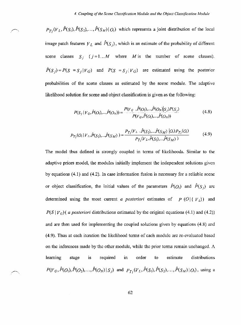
4. Coupling of the Scene Classification Module and the Object Classification Module
PT/V L, peSt), P(S2),"" P(SM) 1 oJ which represents a joint distribution of the local
image patch features V Land P(S j)' which is an estimate of the probability of different
scene classes S j ( j = 1. .. M where M is the number of scene classes).
P(S j) = P(S = S j 1 V c) and P(S = S j 1 V c) are estimated using the posterior
probabilities of the scene classes as estimated by the scene module. The adaptive
likelihood solution for scene and object classification is given as the following:
(4.8)
(4.9)
The model thus defined is strongly coupled in terms of likelihoods. Similar to the
adaptive priors mode1, the modules initially implement the independent solutions given
by equations (4.1) and (4.2). In case information fusion is necessary for a reliable scene
or object classification, the initial values of the parameters P(OJ and P(S) are
determined using the most CUITent a posteriori estimates of P (0 1 { V L} ) and
P(S 1 V G)( a posteriori distributions estimated by the original equations (4.1) and (4.2))
and are then used for implementing the coupled solutions given by equations (4.8) and
(4.9). Thus at each iteration the likelihood terms of each module are re-evaluated based
on the inferences made by the other module, while the prior terms remain unchanged. A
leaming stage IS required III order to estimate distributions
62
4. Coupling of the Scene Classification Module and the Object Classification Module
training set of images for which F(OJ and F(S) have been determined usmg
equations (4.1) and (4.2). The estimation of the probab ility distribution PCV GiS)
involves leaming the characteristics of the feature clusters which represent scene classes
S j. For the probability distribution PCV G, F(OI)' F(Oz),···, peON) 1 S j)' the clusters
formed in the joint space of V Gand P(Oi), not only depict the variability of the
features V G for different scene classes S j' but also depict the relationship between
different object classes Di and the scene classes S j. The clusters representing features
from images belonging to different scene class S j have peaks close to those values of
parameters P(oJ which represent object classes Di that are often found in relationship
with scene class Similarly for the probability distributions
Pr/VL,P(SI),P(SZ), ... ,P(SM) 1 Di), the clusters formed in the joint space of VL and
P(S j) not only depict the variability of the features V L of the image patches of scale
Tl which contain an object from class Di' but also depict the relationship between the
different scene classes S j and the object classes Di. The feature clusters representing
patches containing Di have peaks (are most dense) close to those values of parameters
P(S j) which represent scene classes S j that most often contain objects Di.
63

5. Experimental Resultsfor the Strongly Coupled Scene and Object Classification Models
Chapter 5
Experimental Results for the Strongly Coupled Scene and Object Classification Models
In this chapter we present the experimental results from implementing the strongly
coupled scene and object classification mode!s presented in sections 4.3 and 4.4. We
demonstrate se!ected examples where the scene module or the object module cannot
perform the scene or the object classification task reliably when they function
independently, but where the strong coupling of the two modules improves the initial
classification results. We demonstrate how the initial inferences made about the scene
and the object classes change as the scene module interacts with the object module, and
as the prior model estimations or the likelihood mode! estimations vary in time. We also
measure the performance of the strongly coupled models as classification tools using
receiver operating characteristic (ROC) curves.
In section 5.1 we give a description ofthe database we created for the purpose of
the experiments. In section 5.2 we discuss the choice of sorne important mode!
parameters such as the orientations and scales of the Gabor filters and the number of
Gaussian mixtures used for modeling the likelihood densities based on their effect on the
classification performance. In section 5.3 we demonstrate the effect of the strong
coupling of the two modules on the scene and object classification performance. In this
section we also present the statistical evaluation of the mode! performance and address
the issues of statistical meaningfulness of the presented results. The statistical evaluation
64

5. Experimental Resultsfor the Strongly Coupled Scene and Object Classification Models
of the adaptive priors and the adaptive likelihood models provide a basis for comparing
these two models.
5.1 Experimental Image Database
A database of 1000 natural images from different scene categories was created for the
purpose of these experiments. Each image is 256x256 pixels in size. These images
include pictures taken by a digital camera and images downloaded from the web. The
images have been gathered according to the following scene categories: street scenes,
park scenes, indoor scenes, downtown scenes, and residential (suburban) scenes. The
object classes identified in the images are vehic1es, trees, people, buildings, and
furniture. Sample images of different scene categories are presented in figure (5.1) and
samples of the different object categories are given in figure (5.2).
The images in this database have been gathered under varied times of the year
and different times of the day, and therefore lighting conditions vary among different
images in each scene category. Also there has not been any artificial control ofthe sc ales
in which the objects appear in the scenes. Our goal has been to gather a set of images
that captures the natural frequency of the appearance of different object types in their
different scales, as experienced by the human eye in scenes encountered everyday.
Natural images depicting scenes of the same basic-Ievel categories (such as
forest, mountain, beach, street, buildings, indoors) share common features. According to
the discussion in chapter 2 the study of the power spectrum of the natural images shows
that images belonging to the same basic-Ievel scene categories share common spectral
features, and these features can be used for c1assifying scenes. What gives rise to a
particular spectral shape for a certain scene category is the similarity in the distribution
65

5. Experimental Resultsfor the Strongly Coupled Scene and Object Classification Models
of structural patterns (textures) in scenes of the same category. But the distribution of the
structural patterns and the spectral features of the scene vary based on both the
viewpoint of the observer and also the scale of the images. By scene scale we mean the
mean depth range, i.e. the mean distance between the observers and the elements in the
scene. This issue is important for us, since it sets the constraints for the scene scales and
point ofviews we gather for the database. It is important to consider, for the purpose of
gathering images for the database, how the statistics of the spectral features of the scene
images vary as a function of point of view and mean depth range.
One can intuitively see that the ecological parameters (i.e. parameters that
depend on the interactions between the world and the observer of the world) affecting
the shape of the image power spectra are also strongly constrained by the way scene
images are defined. Although we treat scenes and objects almost in a parallel fashion in
our model, there is an inherent difference between scenes and objects. An object is a
concept that exists independently of the observers' ecological factors, while a scene is a
concept, based on deductions made by the observer, and strongly correlated with the
observers' ecological factors. An object remains the same object, no matter from which
point of view or depth of range it is viewed, while the semantic meaning of an image
viewed by an observer changes when point of view or depth of range changes (the view
of a street by a pedestrian walking in a street and by an airplane passenger flying over
the street do not belong to the same scene category).
With our chosen observer being a human standing up (straight), the viewpoints
for our chosen scene categories (indoors, streets, parks, etc.) are strongly constrained,
with the main components composing the scene also being strongly constrained in
orientation (buildings, cars, trees, furniture, most people) with pronounced horizontal
66

5. Experimental Results for the Strongly Coupled Scene and Object Classification Models
and vertical alignments for most objects. Torralba and Oliva [94] made a study of the
variations of the spectral features of scenes based on changes in the scene scale. Their
results show that significant differences exist between spectral features of images when
the mean depth range changes more than a factor of 10. For the images we have gathered
by digital camera, we controlled the scene scale by maintaining a fixed range of mean
depth for images of the same scene category. Specifically the mean distance of the
observer with the main components of the scene do not vary by more than 10 met ers
from one image to another (no control is used for indoor scenes). The mean depth of the
images collected from the web was controlled by comparing the average scales of the
main components of the scenes, and making them similar to values computed on the
digital camera images.
Ecological constraints, which define a scene category, also constrained the
objects found in the scene. Our database of object patches does not contain an infini te
number of point of views of objects. AIso, the scales of the main objects found in the
scenes are correlated with the scene category. So our database of object patches is
constrained both in point of view and scale. Therefore we do not require an object
classification system (or set of object features) which is spatially invariant or scale
invariant.
67
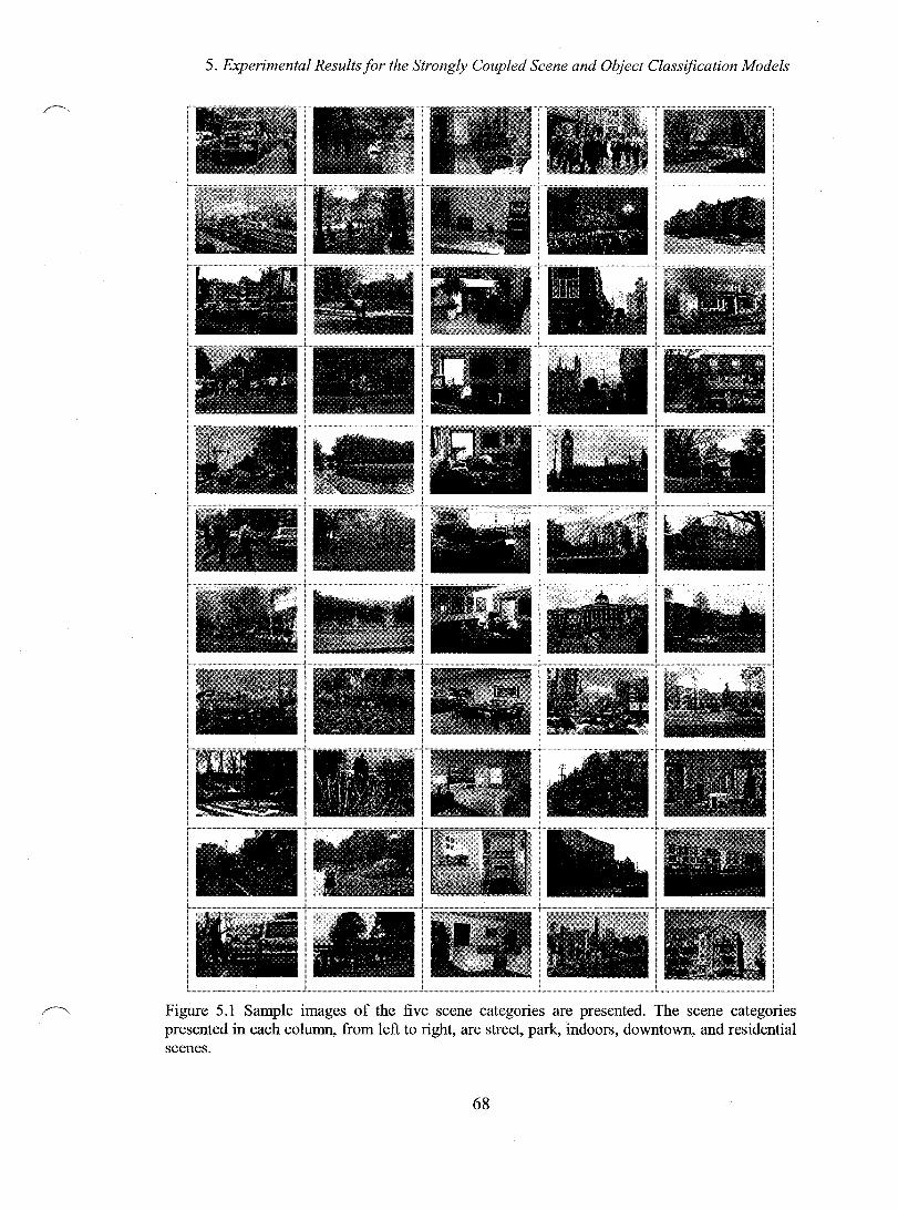
5. Experimental Resultsfor the Strongly Coupled Scene and Object Classification Models
~ 1 < 1\ . " ~,
'tit'i\A... ,#
~,..~ "
Figure 5.1 Sample images of the five scene categories are presented. The scene categories presented in each column, from left to right, are street, park, indoors, downtown, and residential scenes.
68
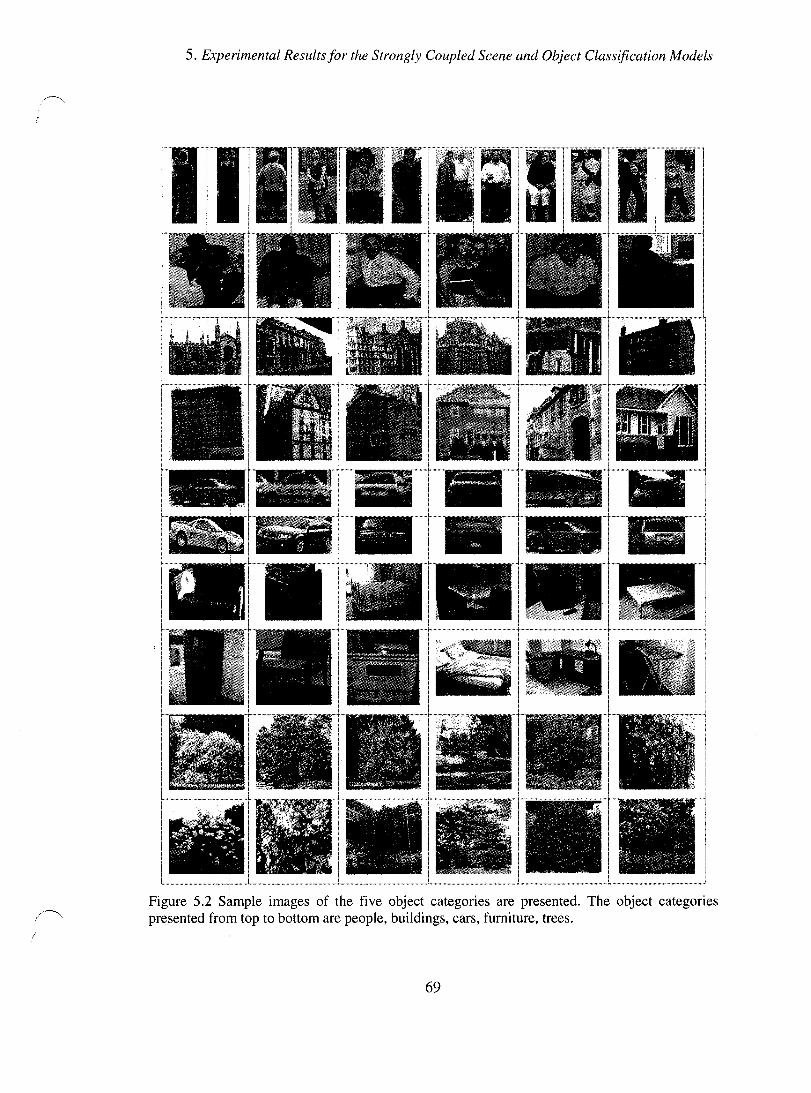
5. Experimental Resultsfor the Strongly Coupled Scene and Object Classification Models
Figure 5.2 Sample images of the five object categories are presented. The object categories presented from top to bottom are people, buildings, cars, furniture, trees.
69
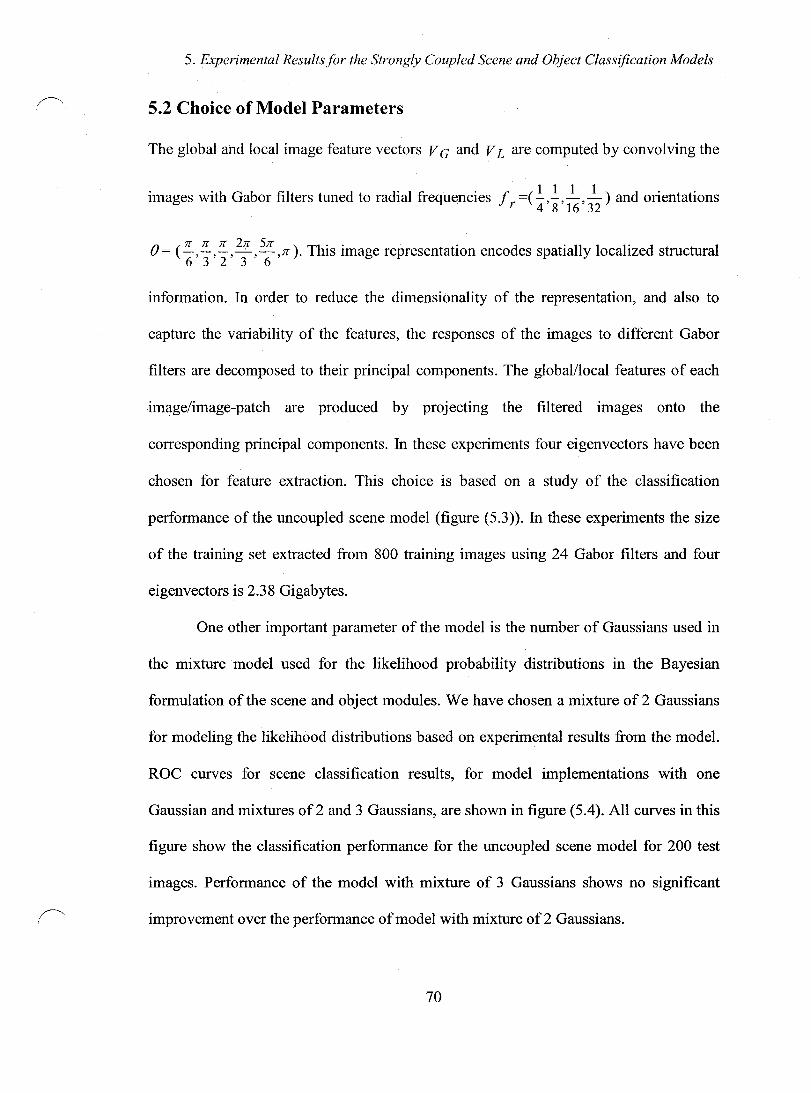
5. Experimental Resultsfor the Strongly Coupled Scene and Object Classification Models
5.2 Choice of Model Parameters
The global and local image feature vectors V G and V Lare computed by convolving the
images with Gabor filters tuned to radial frequencies Ir =( ~,~, ~,~ ) and orientations 4 8 16 32
B= (Ir ,!!., Ir, 21r, Sir ,Ir). This image representation encodes spatially localized structural 6 3 2 3 6
information. In order to reduce the dimensionality of the representation, and also to
capture the variability of the features, the responses of the images to different Gabor
filters are decomposed to their principal components. The global/local features of each
image/image-patch are produced by projecting the filtered images onto the
corresponding principal components. In these experiments four eigenvectors have been
chosen for feature extraction. This choice is based on a study of the classification
performance of the uncoupled scene model (figure (5.3»). In these experiments the size
of the training set extracted from 800 training images using 24 Gabor filters and four
eigenvectors is 2.38 Gigabytes.
One other important parameter of the model is the number of Gaussians used in
the mixture model used for the likelihood probability distributions in the Bayesian
formulation of the scene and object modules. We have chosen a mixture of2 Gaussians
for modeling the likelihood distributions based on experimental results from the model.
ROC curves for scene classification results, for model implementations with one
Gaussian and mixtures of2 and 3 Gaussians, are shown in figure (5.4). AlI curves in this
figure show the classification performance for the uncoupled scene model for 200 test
images. Performance of the model with mixture of 3 Gaussians shows no significant
improvement over the performance of model with mixture of 2 Gaussians.
70
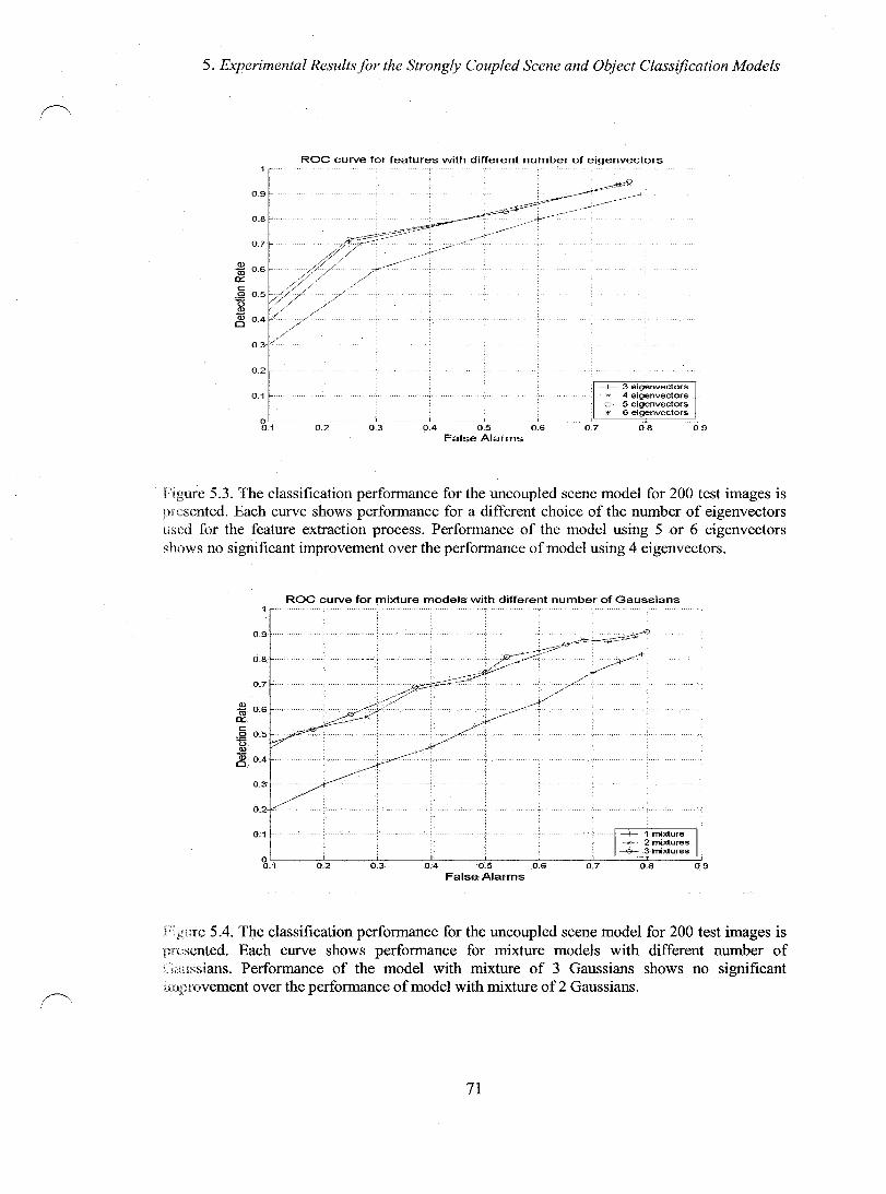
5. Experimental Resultsfor the Strongly Coupled Scene and Object Classification Models
0.2
0.1
ROC curve for features with different number of eigenvectors
-+- 3 eigenvectors "' ~*- 4 eigenvectors
-e- 5 eigenvectors --*--- 6 eigenvectors
oL-____ ~----~L-----~----~~----~----~~====~====~ 0.1 0.2 0.3 0.4 0.5 0.6 0.7 0.8 0.9
False Alarms
Figure 5.3. The classification performance for the uncoupled scene model for 200 test images is prcscnted. Each curve shows performance for a different choice of the number of eigenvectors uscd for the feature extraction process. Performance of the model using 5 or 6 eigenvectors shows no significant improvement over the performance of model using 4 eigenvectors.
0.9
0.8
0.7
"* 0.6 0:: s::: 1 :.:
0.3
0.1
ROC curve for mixture models with different number of Gaussians
o~--~~----~----~~--~~--~~--~~~==~====~ 0.1 0.2 0.5 0.7 0.9 False Alarms
Figure 5.4. The classification performance for the uncoupled scene model for 200 test images is presented. Each curve shows performance for mixture models with different number of (';Iussians. Performance of the model with mixture of 3 Gaussians shows no significant i Ct ~ Ipmvement over the performance of model with mixture of 2 Gaussians.
71

5. Experimental Resultsfor the Strongly Coupled Scene and Object Classification Models
5.3 Experimental Results for the Strongly Coupled Scene and Object Modules
Having discussed the issues of the creation of the database and the choice of important
parameters affecting the model performance, we now present the experimental results
from the implementation of the adaptive priors and the adaptive likelihoods models as
presented in chapter 4. In section 5.3.1 we present selected examples of the models'
behaviors for chosen images of the test set. For each model we have chosen 7 examples
which represent different types of the behavior of the model under a variety of input
images. By studying the behavior of the model in these sample cases we intend to gaina
deeper understanding of the model function and also to examine how the information
flow between the two modules will affect the inferences made by each module. These
cases represent selective behaviors of the model, so a statistical study which measures
the general performance of model as a classification tool is presented in section 5.3.2.
ROC curves which present the performance of the two models for varying decision
thresholds are presented in section 5.3.2.
AIl images in the database have been labeled by 3 human observers. The
observers have been asked to label the images by one of the five scene category labels:
street scene, downtown area, residential area, indoors, and park. The observers have also
been asked to label the patches containing objects as representing one of the 5 object
categories: vehic1es, plants, buildings, fumiture, and people. The scene images left
uncategorized or categorized as ambiguous by at least one of the observers have been
discarded from the database and replaced by non-arnbiguous images, so aIl the images in
the database are uniquely assigned to one of the 5 scene categories by aIl 3 observers
(exarnples of images which have arnbiguous class assignrnents by human observers are
72

5. Experimental Resultsfor the Strongly Coupled Scene and Object Classification Models
kept for sorne experiments, but are not included in the training or the test sets unless
mentioned in the experiments.) The same strategy has also been taken with object
images. Image patches left uncategorized or categorized as ambiguous by at least one of
the observers have been discarded and replaced, so that aIl image patches used for the
training of the object module are uni quel y assigned to one of the 5 object categories by
aIl 3 observers.
For the purpose of these experiments we divided the database of images into 800
images for training and 200 images for testing. Equal numbers of images are used for
training the modules for different scene or object categories. In order to be able to
estimate confidence levels for statistical analysis of the classification results, we have
chosen the strategy of rotating the test set, i.e. at each trial, alternative subsets of the
image database are chosen as test images, and the scene and object modules are trained
using the remaining 800 images in the database. Five different subsets of the database
have been used to compute the confidence levels in the classification results. The mean
standard deviation error is computed for the classification results obtained from each
rotating training image set.
Once a test image is given to the model, the model classification result faIls into
one of the following three categories: correctly classified, misclassified, and unclassified
images. The results of classification are a function ofboth the iteration number and also
the threshold levels we choose for accepting the probability levels as a correct decision.
The image category label given by the human observers is used as the criteria for
validating the model classification results. We specify our exact definition of an image
being correctly classified, unclassified, and misclassified by the model at each section.
73
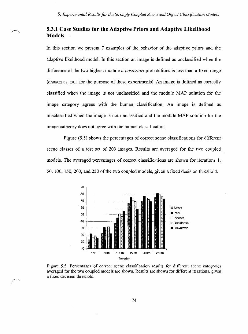
5. Experimental Resultsfor the Strongly Coupled Scene and Object Classification Models
5.3.1 Case Studies for the Adaptive Priors and Adaptive Likelihood Models
In this section we present 7 examples of the behavior of the adaptive priors and the
adaptive likelihood model. In this section an image is defined as unclassified when the
difference of the two highest module a posteriori probabilities is less than a fixed range
(chosen as ±O.1 for the purpose ofthese experiments). An image is defined as correctly
classified when the image is not unclassified and the module MAP solution for the
image category agrees with the human classification. An image is defined as
misclassified when the image is not unclassified and the module MAP solution for the
image category does not agree with the human classification.
Figure (5.5) shows the percentages of correct scene classifications for different
scene classes of a test set of 200 images. Results are averaged for the two coupled
models. The averaged percentages of correct classifications are shown for iterations 1,
50, 100, 150,200, and 250 of the two coupled models, given a fixed decision threshold.
: 1--------------------------------_a_,----
70 1-----~-1
60 -1-'----------------
i 50+----~-------~-~
40 +----------.
30
20 +-1~,--
10
o 1st 50th 100th 150th 200th 250th
Iteration
œStreet
• Park
Olndoors
o Residenlial
• Downlown
Figure 5.5. Percentages of correct scene classification results for different scene categories averaged for the two coupled models are shown. Results are shown for different iterations, given a fixed decision threshold.
74
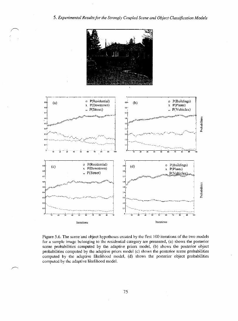
5. Experimental Resultsfor the Strongly Coupled Scene and Object Classification Models
0.& (a) 0.8 .
0.7
0.9 (c)
o P(Residential) x P(Downtown) .. P(Street)
o P(Residential) x P(Downtown) .. P(Street)
Iterations
09 (b) 0.6
0.7
0.2 .......... , .. ...... 0.1 . ., ........... , .
Iterations
o P(Buildings) x P(Plants) .. P(Vehicles)
. ........... . . ........ .
Figure 5.6. The scene 'and object hypotheses created by the first 100 iterations of the two models for a sample image belonging to the residential category are presented, (a) shows the posterior scene probabilities computed by the adaptive priors model, (b) shows the posterior object probabilities computed by the adaptive priors model (c) shows the posterior scene probabilities computed by the adaptive likelihood model, (d) shows the posterior object probabilities computed by the adaptive likelihood mode\.
75
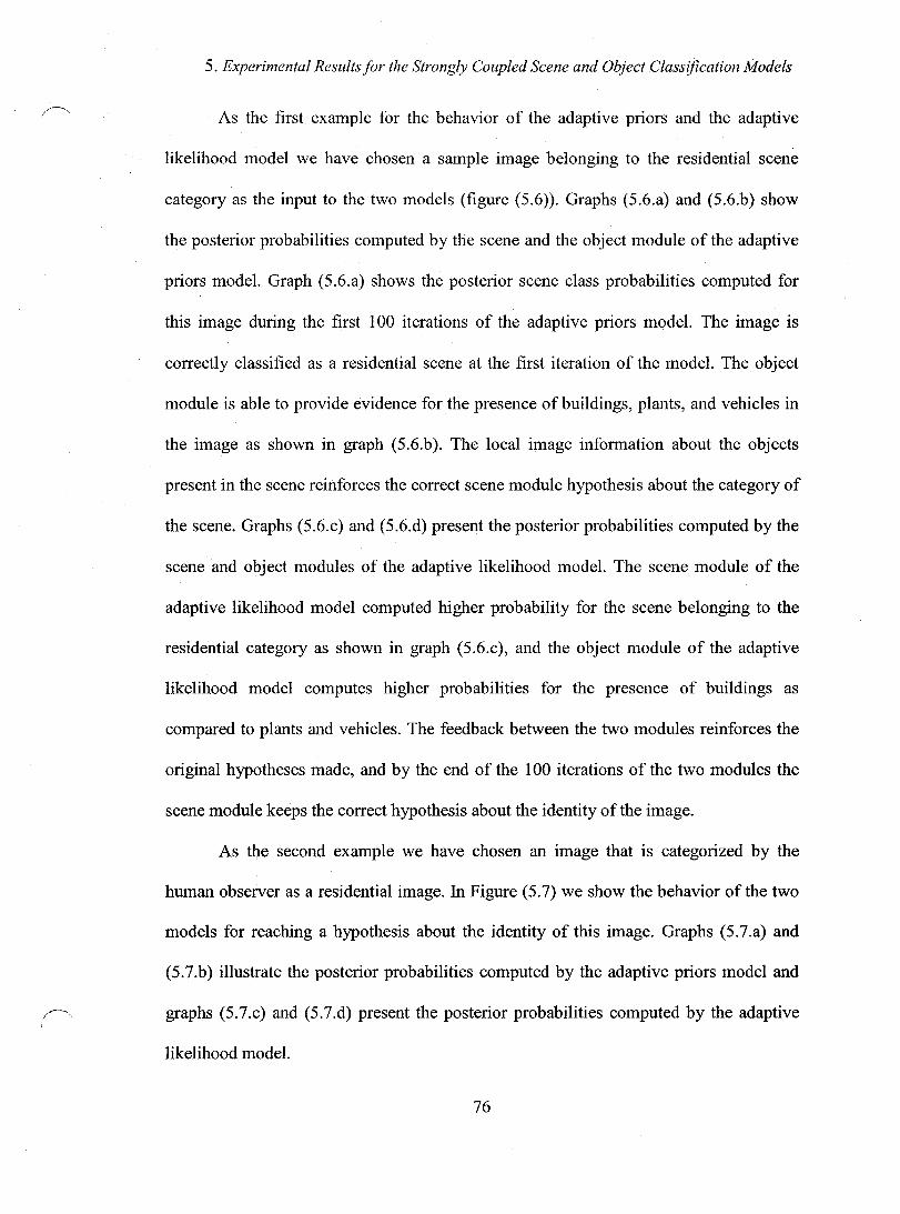
5. Experimental Resultsfor the Strongly Coupled Scene and Object Classification Models
As the first example for the behavior of the adaptive priors and the adaptive
likelihood model we have chosen a sample image belonging to the residential scene
category as the input to the two models (figure (5.6)). Graphs (5.6.a) and (5.6.b) show
the posterior probabiIities computed by the scene and the object module of the adaptive
priors model. Graph (5.6.a) shows the posterior scene class probabiIities computed for
this image during the first 100 iterations of the adaptive priors model. The image is
correctly classified as a residential scene at the first iteration of the model. The object
module is able to provide evidence for the presence of buildings, plants, and vehicles in
the image as shown in graph (5.6.b). The local image information about the objects
present in the scene reinforces the correct scene module hypothesis about the category of
the scene. Graphs (5.6.c) and (5.6.d) present the posterior probabilities computed by the
scene and object modules of the adaptive likelihood model. The scene module of the
adaptive likelihood model computed higher probability for the scene belonging to the
residential category as shown in graph (5.6.c), and the object module of the adaptive
likelihood model computes higher probabilities for the presence of buildings as
compared to plants and vehicles. The feedback between the two modules reinforces the
original hypotheses made, and by the end of the 100 iterations of the two modules the
scene module keeps the correct hypothesis about the identity of the image.
As the second example we have chosen an image that is categorized by the
human observer as a residential image. In Figure (5.7) we show the behavior of the two
models for reaching a hypothesis about the identity of this image. Graphs (5.7.a) and
(5.7.b) illustrate the posterior probabilities computed by the adaptive priors model and
graphs (5.7.c) and (5.7.d) present the posterior probabilities computed by the adaptive
likelihood model.
76
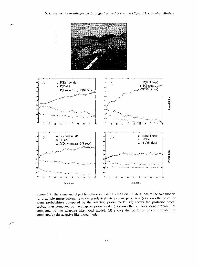
(
5. Experimental Resultsfor the Strongly Coupled Scene and Object Classification Models
09 (a)
0.8
o.,
0.9 (c) 0.8
0.3
0.2 ....
........... 0.1
o P(Residential) x P(Park) .. P(Downtown)+P(Street)
o P(Residentiad x P(Park)
P(Downtown)+P(Street)
........................................... , .. ............................
Iterations
... , ..... "
0.1
""'" ........... " ..... . 10 20 30 40 50 60
0.9 (d) 0.8
O"l 0.6
o P(Buildings) x P(Plants) .. P(Vehicles)
1 T~ ~. 0.5 [ ~,o""",,';\'\' lQj}K'xi0i&<,o.",9f"lJ'''''è,b"" '{;<,,,cçe"""'''Q
0 .. '(9"" " ~. 1"< "~'" w. :J ........ : .. :.:::::::::::::::::=::::::::::::=:::~ w • ~ ~ w ~ ro ~ 00 a
Iterations
Figure 5.7. The scene and object hypotheses created by the first 100 iterations of the two models for a sample image belonging to the residential category are presented, (a) shows the posterior scene probabilities computed by the adaptive priors mode), (b) shows the posterior object probabilities computed by the adaptive priors model (c) shows the posterior scene probabilities computed by the adaptive likelihood model, (d) shows the posterior object probabilities computed by the adaptive likelihood mode\.
77

~"
5. Experimental Resultsfor the Strongly Coupled Scene and Object Classification Models
Graph (5.7.a) illustrates the a posteriori probabilities orthe test image belonging
to the residential category or the park category, as produced by the scene module, for the
first 100 iterations of the adaptive priors model. The image is unclassified by the scene
module at the first iteration of the model since the difference of the probabilities of the
scene belonging to the residential or the park category is less than 0.1 . The three curves
in graph (5.7.b) illustrate the a posteriori probabilities of image containing buildings,
plants, and vehicles, as produced by the object module, at the first 100 iterations of the
adaptive priors model. The scene probabilities estimated by the first iteration of the scene
module are in fact the results of scene categorization without any feedback from the
object module. One can interpret the model behavior as the following: At the first
iteration, the scene module is not able to discriminate between the image global features
V G belonging to the residential category or the park category. The object module finds
evidence for buildings, plants, and vehicles in the scene. This combination of objects,
with their relative probability levels, provide an object profile which modifies the prior
model of the scene module in a way which favors the probability of image being a
residential scene versus a park scene. At the same time the scene a posteriori distribution
propagates to the object module, and modifies the prior model of the object module. The
modification of the object priors has the effect of changing the original hypothesis made
about sorne of the object patches, and the aggregation of these changes pro duces new
estimates for the probability of presence of buildings, plants, or vehicles in the image.
After 100 iterations, the mutual feedback between the scene and the object module has
the overall effect of increasing the probability of the scene belonging to the residential
category as compared to the park scene. At the end of the 100th iteration more patches
78

5. Experimental Resultsfor the Strongly Coupled Scene and Object Classification Models
have been labeled as buildings, and with higher probabilities, as the probability level of
the presence of buildings has increased as compared to plants, or vehicles.
Graphs (5.7.c) and (5.7.d) in this example show the posterior probabilities
computed by the scene and the object module of the adaptive likelihood model. Graph
(5.7.c) shows the probability of the scene belonging to the residential or the park
category as computed by the adaptive likelihood model. The scene module with no
feedback computes similar probabilities for the scene being a residential or a park scene.
The likelihood term of the scene module with no feedback computes the likelihood of the
scene belonging to different scene categories based only on the global context features of
the image V G. The strong coupling of the likelihood terms of the two modules has the
effect of increasing the probability of the scene belonging to the residential category. The
likelihood term of the scene module with feedback computes the likelihood of the scene
belonging to different scene categories based on the joint probability density of the
global context features V G and the probability of the presence of different object
categories such as buildings, plants, and vehicles. Similarly, the likelihood term of the
object module with no feedback computes the likelihood of the presence of different
object categories based only on the local features v L • The likelihood term of the object
module with feedback computes the likelihood of the presence of different object
categories based on the joint probability density of the local features V L and the
probability of the image belonging to different scene categories. The joint scene
likelihood function estimates higher probabilities for the image belonging to the
residential scene category. The joint object likelihood function estimates higher
probability for patches containing buildings.
79
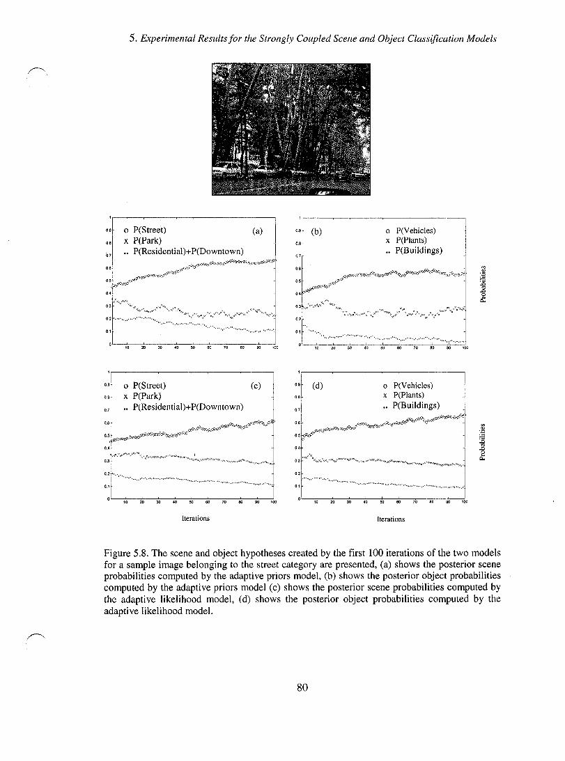
5. Experimental Resultsfor the Strongly Coupled Scene and Object Classification Models
09 0 P(Street) 08r x P(Park)
(a)
o,f .. P(ResidentiaI)+P(Downtown) i .çCÎ:f,~oJr,.-)}-Q2"~;-I\..çQ"Çf..( ... ~·O:t:O<-t(-tf)'~.pt
o.sr :-Ç1'(qflj-#'-! ÇS'Cf>fO n:r ((:>Î)J"
05r~Ç;
'r 0'1 O.3~l(x",,*,\wx" x'<./>'x ~ 0.2~ ............. :::~::::::: '~""""~\(,*,/ •• <r/,,,,.~/r",········"Y·".'·x
O.,
l
rl ................... , ...... " ••• , ............... . .........
OL-~'O--~2LO--W~~.o--~w--~~~~,LO--~ .. --~oo--~'oo
09
0.8
0.7 .
o .•
0.3
o P(Street) (c) x P(Park)
P(ResidentiaI)+P(Downtown)
0.2 ................................................................................. . 0.1 .............. .
Iterations
0.9 (b)
0.8
0.7 -
0.2
o P(VehicJes) x P(Plants) .. P(Buildings)
0:[ ..... : ................... : ......... : ......... ; ............................. : .................. . w • ~ • M .. ro .. 00 _
o:r (d) 0 P(Vehicles) O'r x P(Plants)
1 P(Buildings) o'f
1 ~.~"",,,,~ 06,· r~~"'G'"
::llo~~ . w"
0.3" lo:lIxxx" \x/~y'<X>(>(""XX)(>O(""x>!'4""»)<X"x'XX><"y,..x)(1<':.,,'XI<~~XX><>i<~""~l<!'<"""'>O<>«"~,~"">:yl'
0.2 ...................... o., . ............................................................... .
Iterations
Figure 5.8. The scene and object hypotheses created by the first 100 iterations of the two models for a sample image belonging to the street category are presented, (a) shows the posterior scene probabilities computed by the adaptive priors model, (b) shows the posterior object probabilities computed by the adaptive priors model (c) shows the posterior scene probabilities computed by the adaptive likelihood model, (d) shows the posterior object probabilities computed by the adaptive likelihood mode\.
80

5. Experimental Resultsfor the Strongly Coupled Scene and Object Classification Models
Figure (5.8) presents an example for the behavior of the two adaptive models for
an image that is categorized by the hum an observer as belonging to the street category.
Graph (5.8.a) illustrates the a posteriori probabilities of the test image belonging to the
street category or the park category, as produced by the scene module of the adaptive
priors mode!. The three curves in graph (5.8.b )illustrate thea posteriori probabilities of
image containing vehicles, plants, and buildings, as produced by the object module of
the adaptive priors mode!. The global image features V G do not provide adequate
evidence for the scene module to independently produce a reliable hypothesis about the
identity of the image, and in the first iteration, the scene module estimates very close
probability values for the image being a street scene or a park scene. The object module
is able to independently find evidence for vehicles, plants, and buildings in the scene, as
presented in the first object a posteriori estimates. The feedback between the two
modules has the effect of the enforcement of the hypothesis of the image being a street
scene and the weakening of the hypothesis of the image being a park scene.
Each scene class is associated with a prototypical arrangement of objects. The
strong coupling of the scene priors and the object priors in fact makes an association
between each scene class and its prototypical arrangement of objects. When the object
posterior probabilities are projected to the scene module the set of associations that
correspond to the relevant scene context are activated and result in an enforcement of the
posterior probability of the scene class which is most strongly associated with the
present set of objects. In this example the profile of the objects in the scene, a high
probability of vehicles and lower probabilities for plants and buildings enforces the
hypothesis of the image being a street scene. When the higher probability of image being
81
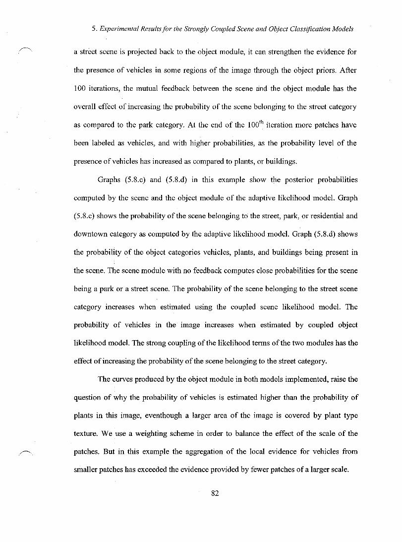
5. Experimental Resultsfor the Strongly Coupled Scene and Object Classification Models
a street scene is projected back to the object module, it can strengthen the evidence for
the presence of vehicles in sorne regions of the image through the object priors. After
100 iterations, the mutual feedback between the scene and the object module has the
overall effect of increasing the probability of the scene belonging to the street category
as compared to the park category. At the end of the 100th iteration more patches have
been labeled as vehicles, and with higher probabilities, as the probability level of the
presence of vehi cl es has increased as compared to plants, or buildings.
Graphs (5.8.c) and (5.8.d) in this example show the posterior probabilities
computed by the scene and the object module of the adaptive likelihood model. Graph
(5.8.c) shows the probability of the scene belonging to the street, park, or residential and
downtown category as computed by the adaptive likelihood model. Graph (5.8.d) shows
the probability of the object categories vehicles, plants, and buildings being present in
the scene. The scene module with no feedback computes close probabilities for the scene
being a park or a street scene. The probability of the scene belonging to the street scene
category increases when estimated using the coupled scene likelihood model. The
probability of vehicles in the image increases when estimated by coupled object
likelihood model. The strong coupling of the likelihood terms of the two modules has the
effect of increasing the probability of the scene belonging to the street category.
The curves produced by the object module in both models implemented, raise the
question of why the probability of vehicles is estimated higher than the probability of
plants in this image, eventhough a larger area of the image is covered by plant type
texture. We use a weighting scheme in order to balance the effect of the scale of the
patches. But in this example the aggregation of the local evidence for vehicles from
smaller patches has exceeded the evidence provided by fewer patches of a larger scale.
82
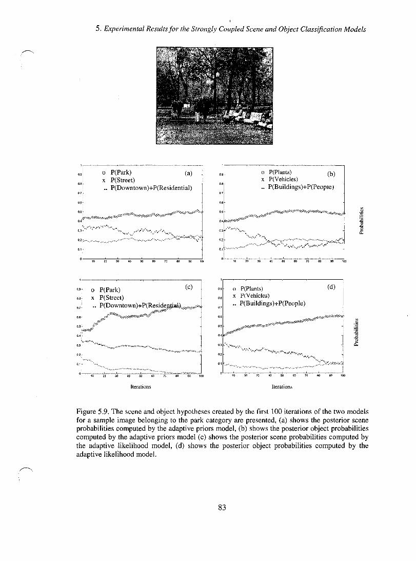
5. Experimental Resultsfor the Strongly Coupled Scene and Object Classification Models
1" ____________ . __________________ ,
09~ 08
1
i 0.7i"
i
o P(Park) (a) x P(Street) •. P(Downtown)+P(Residential)
o ''---::10:----:':--0 ---:3=-0 --7::'0--:':50,----=60:----:7::-0 -.=-0 ---:':90--~'0(
0.9 0 P(Park) (c)
o .• x P(Street)
0.7 P(Downtown)+ P(Reside ,~>5è6'l.\
0.6
o.,
0.1 r " .... ""." ......... " .................. " .. . 0'----=1O:--~'::-0--3=-0---:':40---:':50:----:60:--.. _ .. ·~,·;~~·~"~· ~.0~~90~~,00
Iterations
o P(Plants) (b) x P(VehicIes)
09
0.8 .. P(Buildings)+P(Peopw)
07
0.6
10
O:~('PlantS) (d)
081 x :~vehicIeS) .. P(Buildings)+P(People)
0.7
0,1 •
10 20 30 .0 90 100
Iterations
Figure 5.9. The scene and object hypotheses created by the first 100 iterations of the two models for a sample image belonging to the park category are presented, (a) shows the posterior scene probabilities computed by the adaptive priors model, (b) shows the posterior object probabilities computed by the adaptive priors model (c) shows the posterior scene probabiIities computed by the adaptive likelihood model, (d) shows the posterior object probabilities computed by the adaptive likelihood mode!.
83
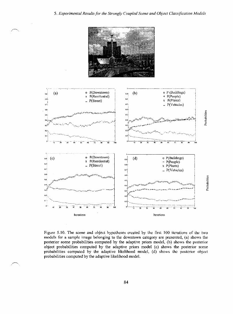
5. Experimental Resultsfor the Strongly Coupled Scene and Object Classification Models
Ogr
0.8!-
t o.rf
i
(a) o P(Downtown) x P(Residential)
P(Street)
O,6r'
1 {<>_~'9':'-.((Z,S"!."~..:6l:.:.;t~J/~.(ù.nr,;);\t'{(f>-·:4m).v>o.U.f9t 0.5! ~ -o.M-'(J'('O .. -{4b;19}}-· "1
i ~_' i o .• b,)(~" " , /,,:,"jf
T _~; ~ ,<'." ''''" .... l<'-K,,'' /.,( p~.>«. j
O.3t~ '~><...-'>t-c< /·x,./,r··""':>",,/ ·"'.A~;':<,.,/.~'<"-,.,/x,,,,,,,x,,t>;'''/,,y'?(,x. -
1
02+-.
011'" ........................ . 1 ..... • ........ ..
oL_.....!..-___ .~....l...- ·:.::.:.::..~.·.;.L .. '-....... _ .. __ ..... _____ j W W ~ W ~ 00 ro W 00 _
.........
o P(Downtown) x P(Residential) •• P(Street)
! o L ..... __ . .i... ___ -'-_.__ '., ," ...... , ••• " .......... "., ' •••••••• ' ,,, •••• , ' ••••• " .. ,."
10 20 ··"3Q-"40-··-···-S0---·,,··6ë---ro"M-----OO100
Iterations
o P (Buildings) + P(People) x P(Plants)
P(Vehicles)
'r---------~ __ --------------------,
=1 (d)
O.7~
o P(Buildings) + P(People) x P(Plants) •• P(Vehicles)
Iterations
Figure 5.10. The scene and object hypotheses created by the first 100 iterations of the two models for a sample image belonging to the downtown category are presented, (a) shows the posterior scene probabilities computed by the adaptive priors model, (b) shows the posterior object probabilities computed by the adaptive priors model (c) shows the posterior scene probabilities computed by the adaptive likelihood model, (d) shows the posterior object probabilities computed by the adaptive likelihood model.
84
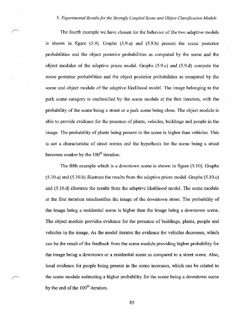
5. Experimental Resultsfor the Strongly Coupled Scene and Object Classification Models
The fourth exarnple we have chosen for the behavior of the two adaptive models
lS shown in figure (5.9). Graphs (5.9.a) and (5.9.b) present the scene posterior
probabilities and the object posterior probabilities as computed by the scene and the
object modules of the adaptive priors model. Graphs (5.9.c) and (5.9.d) compute the
scene posterior probabilities and the object posterior probabilities as computed by the
scene and object module of the adaptive likelihood model. The image belonging to the
park scene category is unclassified by the scene module at the first iteration, with the
probability of the scene being a street or a park scene being close. The object module is
able to provide evidence for the presence of plants, vehicles, buildings and people in the
image. The probability of plants being present in the scene is higher than vehicles. This
is not a characteristic of street scenes and the hypothesis for the scene being a street
becomes weaker by the 100th iteration.
The fifth example which is a downtown scene is shown in figure (5.1 0). Graphs
(5.1O.a) and (5.10.b) iIlustrate the results from the adaptive priors model. Graphs (5.10.c)
and (5.1O.d) iIlustrate the results from the adaptive likelihood model. The scene module
at the first iteration misclassifies the image of the downtown street. The probabiIity of
the image being a residential scene is higher than the image being a downtown scene.
The object module provides evidence for the presence of buildings, plants, people and
vehicles in the image. As the model iterates the evidence for vehicles decreases, which
can be the result of the feedback from the scene module providing higher probability for
the image being a downtown or a residential scene as compared to a street scene. AIso,
local evidence for people being present in the scene increases, which can be related to
the scene module estimating a higher probability for the scene being a downtown scene
by the end of the 100th iteration.
85
~"
5. Experimental Resultsfor the Strongly Coupled Scene and Object Classification Models
0.9 0 P(Indoors) (a) li 0.8 X P(Park) 0.7 •• P(Street)+P(Residential)+P(Downtown)
06
o 5 ~#.::fJ'..zv->-wü.<......-.:c-I))T(\V-~p:n::(;~pi~~:(~S:flS.')J)lj
û"p61~C" '" .<,;«
o. x"X'<.,,:"'" :.<:,,"xq .... ><xl"" x~x><::<>("r"',.>O<"",,"" )<,,~,,;< ,,~x,."'»./"'x..,.;..,..)<y\'xx,./<x,,~><~;.)<><"'" 0.3 "y''>:x/~»" •
0.2 ".
0.1 ......... . .......... . ....................... ............
o _----.J...-.... __ J. __ L_. ___ I..._~_._~---L~ __ L-_
W ~ • • ~ w ro w 00 w
0.9 0 P(Indoors) ( C )
08 X P(Park) 0.7 •• P(Street)+P(Residential)+P(Downtown)
«<>û.
6"'J~"Q~<V 0.5 cr?o;>S0
0.6
O··~*"'W"""",="""_,""",,<,,,,,,~~Y<"""~""'*""""""""""" 0.3 ,.=- """"'~'~"""""=<"'~'»'~'od
02
0.1 ......................
Iterations
0.9 0 P(Fumiture) (b) 0.8 x P (Plants) 0.7 •• P(Buildings)+ P(Vehic1es)
02
0.1 ",
0.9 0 P(Fumiture) x P(Plants) 0.8
0.7 .• P(Buildings)+ P( Vehic1es)
0.3
0.2
0.1 •••••••
(d)
o --~ ·:········;,········i··~·····ï·····~ ...... ·.l· .... ·.",. "-Lo.
10 20 • • ~ w ro w w ~
Iterations
Figure 5.11. The scene and object hypotheses created by the flfst 100 iterations of the two models for a sample image belonging to the indoors category are presented, (a) shows the posterior scene probabilities computed by the adaptive priors model, (b) shows the posterior object probabilities computed by the adaptive priors model (c) shows the posterior scene probabilities computed by the adaptive likelihood model, (d) shows the posterior object probabilities computed by the adaptive likelihood model.
86
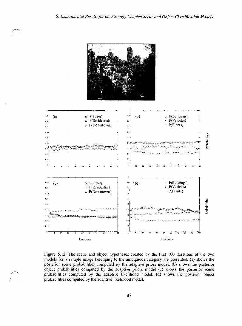
.~.
!
5. Experimental Resultsfor the Strongly Coupled Scene and Object Classification Models
0.9
oef
0'1
::~
(a) o P(Street) x P(Residential) .. P(Downtown)
o"l'""'~'~~~~~~ 0,3 :.y"><"xy~:'!,,y''':'O<'\..X ''*'',/' ..... '~":'-H"", ... ",··1:,<)ol."'~·X"'·''(''';l\VU''''''''''''''''f."')1,
0'>
01 f OL
I ~~~~~~--~~~~--=-~~~ 10 20 30 40 50 60 70 80 90 10
0.9 (c) 0.8
o.,
06
0.5
o .•
o P(Street) x P(Residential)
P(Downtown)
50 60 70 80 90 100
Iterations
0.9
0.8
0.6·
(b) o P(Buildings) x P(Vehicles) .. P(Plants)
0.5
0·'r()>:'}P:6,(rP~~~,))):9'f:tQJ'éJ'fJtq:fl:)'f.tl:O:o-j.o:G-"'t9J)~i~-Qyo;r;~;-.0-~ "~ ,,""x ">C<.,,,/.z)'\l\Xx.,,/',;«\~~~\/:><.,,; x,.,..,,";'>tx"-y, >; x x<"""Y>I/"x x,..",x""->e><
0.3 '(x x ""x,,.,,/ ~ )Q< '" ~ x";.:x,, X """",<x"
:JV w m w ~ m w ro 00 00 ~
o P(Buildings) x P(Vehicles) .. P(Plants)
, ....................... . . ............... , .. .
Iterations
Figure 5.12. The scene and object hypotheses created by the first 100 iterations of the two models for a sample image belonging to the ambiguous category are presented, (a) shows the posterior scene probabilities computed by the adaptive priors model, (b) shows the posterior object probabilities computed by the adaptive priors model (c) shows the posterior scene probabilities computed by the adaptive likelihood model, (d) shows the posterior object probabilities computed by the adaptive Iikelihood mode!.
87

5. Experimental Results for the Strongly Coupled Scene and Object Classification Models
The sixth example is an image which belongs to the indoor scene category. The
results related to this example are shown in figure (5.11). This image is initially
unclassified by the scene module. The global context features are not adequate for
uniquely classifying this image. This may be due to the large windows in the indoor
image which show plants from outdoors. The object module finds evidence for the
presence of both fumiture and plants in the image. The model is able to resolve the
ambiguity in the scene identity by the 100th iteration, although the rate of increase in the
indoor a posteriori probability levels is not uniform, and the model seems to oscillate
between the indoor and the park identities.
The last example is an ambiguous image in the sense that the human observers
have not been able to uniquely label this image as a street scene, a downtown scene, or a
residential scene (figure (5.12)). It is interesting to show that the model is also unable to
resolve the ambiguity in the scene identity. Evidence is found as for the presence of
buildings, vehicles and plants, but the relative probability levels of the presence of the
object categories do not reinforce a specifie scene prior and the model oscillate between
the three hypotheses.
5.3.2 Statistical Study of the Classification Results
The suggested architectures can be compared from different points of view. In this
section we would limit the criteria of the comparison of the two models to their
performance in classification tasks. Figure (5.13) presents the comparison of the two
models based on their performance in terms of correct classifications of scene identities.
Receiver Operator Curves (ROC) demonstrate the performance of the models in terms of
their true positive and false positive results and can be used as a tool for quantitatively
88
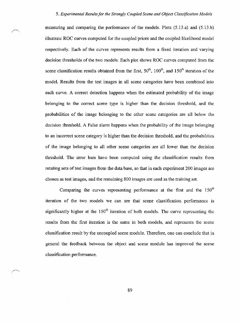
5. Experimental Resultsfor the Strongly Cou pied Scene and Object Classification Models
measuring and comparing the perfonnance of the models. Plots (5.l3.a) and (5.13.b)
illustrate ROC curves computed for the coupled priors and the coupled likelihood model
respectively. Each of the curves represents results from a fixed iteration and varying
decision thresholds of the two models. Each plot shows ROC curves computed from the
scene classification results obtained from the first, 50th, 100th, and 150th iteration of the
model. Results from the test images in an scene categories have been combined into
each curve. A correct detection happens when the estimated probability of the image
belonging to the correct scene type is higher than the decision threshold, and the
probabilities of the image belonging to the other scene categories are an below the
decision threshold. A False alann happens when the probability of the image belonging
to an incorrect scene category is higher than the decision threshold, and the probabilities
of the image belonging to an other scene categories are an lower than the decision
threshold. The error bars have been computed using the classification results from
rotating sets of test images from the data base, so that in each experiment 200 images are
chosen as test images, and the remaining 800 images are used as the training set.
Comparing the curves representing perfonnance at the first and the 150th
iteration of the two models we can see that scene classification perfonnance is
significantly higher at the 150th iteration of both models. The curve representing the
results from the first iteration is the same in both models, and represents the scene
classification result by the uncoupled scene module. Therefore, one can conclude that in
general the feedback between the object and scene module has improved the scene
classification perfonnance.
89
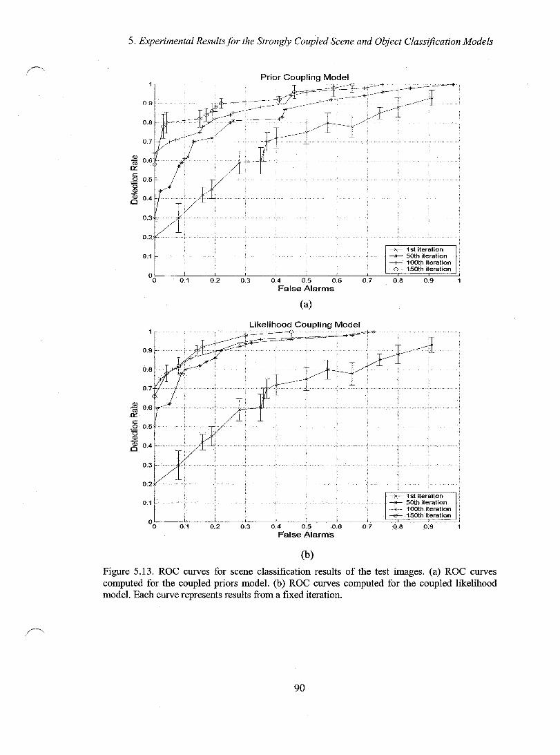
5. Experimental Resultsfor the Strongly Coupled Scene and Object Classification Models
0.2
0.1
°0~--~~----~----~----~OL.4~--~0~.5~---0~.~6----~~~=OI.8=====0~.9====~ False Alarms
(a)
Likelihood Coupling Model ---. ~ ..... ~ ~
0.9
0.1 -><-- 1 st iterati on
... __ 50th iteration -+- 100th iteration -<&- 150th iteration
°0L---~~--~~----0~.L3----~OL.4~·----oi.5~---O~.~6-----0L.7--~=OI.8=====0~.9====~ False Alarms
(h)
Figure 5.13. ROC curves for scene classification results of the test images. (a) ROC curves computed for the coupled priors model. (b) ROC curves computed for the coupled likelihood model. Each curve represents results from a fixed iteration.
90

6. Comparison of the Strongly Coupled Scene and Object Classification Models
Chapter 6
Comparison of the Strongly Coupled Scene and Object Classification Models
In the prevlOUS chapter we presented the experimental results obtained from
implementing the strongly coupled scene and object classification models. The receiver
operating characteristic (ROC) curves depicting the performance of each of the strongly
coupled models (figure 5.13) shows that in general the feedback mechanism between the
object classification module and the scene classification improves the scene
classification performance in both models. In this chapter we further analyze the outputs
obtained from the two models in order to establish sorne of the main characteristics of
the models such as predictability, speed of response, and robustness of the models.
Investigating these questions also provides a basis for comparing the behavior of the two
models. In section 6.1 we compare the classification performance of the two models
using the corresponding ROC curves. In section 6.2 we investigate the predictability of
the two models using cross-correlation plots and in section 6.3 we compare the speed of
the two models by estimating the rise times of the models' outputs. In section 6.4 we
investigate the robustness of the models to variations of the input image such as changes
in image orientations, and additional noise.
6.1 Classification Performance of the Two Models
Plotting the ROC curves representing the scene classification performance of the two
models demonstrates a significant difference in their detection rates. In order to
91
6. Comparison of the Strongly Coupled Scene and Object Classification Models
demonstrate this result more Clearly, we plot the ROC curves obtained from the two
models, for fixed iterations and varying decision thresholds, in the same graph (figure
(6.l.a) and (6.l.b)). In figure (6.l.a) the two curves corresponding to the classification
results obtained from the 50th iteration of the two models are shown. In figure (6.l.b) the
two curves corresponding to the classification results obtained from the 150th iteration of
the two models are shown.
The results depicted III figure (6.l.a) and (6.l.b) show that the adaptive
likelihood model has a higher detection rate as compared to the adaptive priors model.
Based on these experimental results one can empirically conclude that constraining the
likelihoods provides better solutions for the scene classification problem compared to
constraining the priors, given our choice of image features and image data base. This
result also implies that the MAP solutions of the Bayesian estimation problems
presented by the functions of the scene and object modules are more sensitive to changes
in the shape of the likelihood distributions, as compared to changes in the shape of the
priOf distributions.
6.2 Predictability of the Two Models
We use autocorrelation plots as tools for checking the predictability of the model.
Randomness in a data set is ascertained when the autocorrelation plots have near zero
values for all time lag separations. If the data set is non-random one or more of the auto-
correlation values is significantly non-zero. We form the auto-correlation plots by
computing the auto-correlation coefficient Rh as the following
(6.1)
92
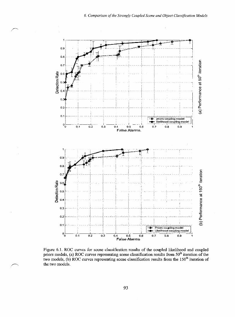
6. Comparison of the Strongly Coupled Scene and Object Classification Models
0.9
0.8
c:: .Q o. 13 (J)
~ 0.4
o.
0.2
0.1
o~--~--~----~--~ ____ ~ __ -i~=======r====r===~
c:: .Q 0.5 13 (J)
~ 0.4
0.1
o 0.1 0.2 0.3 0.4 0.5 0.6 0.7 0.8 0.9
False Alarms
°o~--~-----L----i-----L---~-----L~==~====C====I====~ 0.1 0.2 0.3 0.4 0.5 0.6 0.7 0.8 0.9
False Alarms
c .Q ro L..
:ê = o 1.0 -ro Q) () c ro E .g Q) a..
c o ~ L..
:ê =0 1.0 ..--ro ~ c ro E .g Q) a.. ........ .0 ........
Figure 6.1. ROC curves for scene classification results of the coupled like1ihood and coupled priors mode1s, (a) ROC curves representing scene classification results from 50th iteration of the two models, (b) ROC curves representing scene classification results from the 150th iteration of the two models.
93
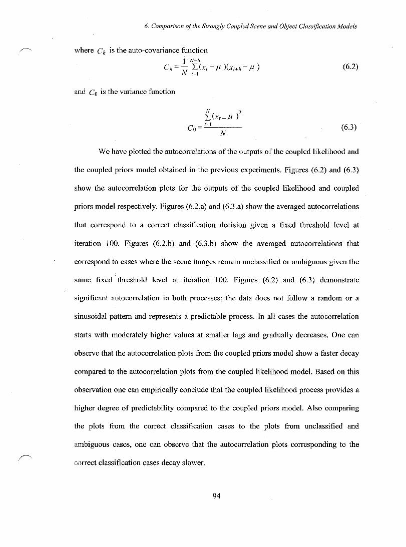
r-'-..
6. Comparison of the Strongly Coupled Scene and Object Classification Models
where Chis the auto-covariance function 1 N-h
Ch = N I~(XI - Ji )(Xt+h - Ji )
and Co is the variance function
N 2 I. (Xt - Ji )
Co = "-.-1=..:....1 ---
N
(6.2)
(6.3)
We have plotted the autocorrelations of the outputs of the coupled likelihood and
the coupled priors model obtained in the previous experiments. Figures (6.2) and (6.3)
show the auto correlation plots for the outputs of the coupled likelihood and coupled
priors model respectively. Figures (6.2.a) and (6.3.a) show the averaged autocorrelations
that correspond to a correct classification decision given a fixed threshold level at
iteration 100. Figures (6.2.b) and (6.3.b) show the averaged autocorrelations that
correspond to cases where the scene images remain unclassified or ambiguous given the
same fixed threshold level at iteration 100. Figures (6.2) and (6.3) demonstrate
significant auto correlation in both processes; the data does not follow a random or a
sinusoidal pattern and represents a predictable process. In aIl cases the autocorrelation
starts with moderately higher values at smaller lags and gradually decreases. One can
observe that the auto correlation plots from the coupled priors model show a faster decay
compared to the auto correlation plots from the coupled likelihood mode!. Based on this
observation one can empirically conclude that the coupled likelihood process provides a
higher degree of predictability compared to the coupled priors mode!. Also comparing
the plots from the correct classification cases to the plots from unclassified and
ambiguous cases, one can observe that the auto correlation plots corresponding to the
correct classification cases decay slower.
94
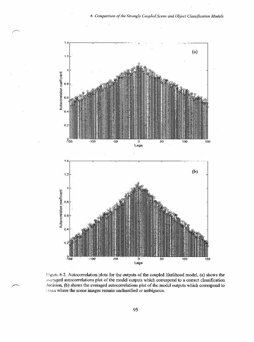
6. Comparison of the Strongly Coupled Scene and Object Classification Models
1.4._-------.---------,--------~--------,_--------._------_,
-c <J)
(> :E
1.2
~ 0.8 o c o
1U ~ 0.6 o o .9 ::l «
-100 -50 o Lags
50 100
(a)
150
1.4,--------,---------,---------,--------,---------,---------
1.2 (b)
hgure 6.2. Autocorre1ation plots for the outputs of the coupled likelihood model, (a) shows the ;;veraged autocorre1ations plot of the model outputs which correspond to a correct classification decision, (b) shows the averaged autocorre1ations plot of the mode1 outputs which correspond to . HSCS where the scene images remain unclassified or ambiguous.
95
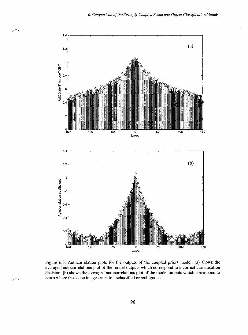
6. Comparison of the Strongly Coupled Scene and Object Classification Models
1.4.-------~--------~--------~--------__ --------__ ------~
~
c Q) '0
1.2
t\jj o 0.8 (.)
c o ~ ~ 0.6 o (.)
~ « 0.4
-100 -50 o Lags
50
(a)
100 150
1.4r--------,---------.--------~--------~--------._------_.
ë Q) ·0
1.2
t\jj 00.8 (.)
c o ~ ~ 0.6
~ ::l «
0.4
-100 -50 o Lags
50
(b)
100 150
Figure 6.3. Autocorrelation plots for the outputs of the coupled priors model, (a) shows the averaged autocorrelations plot of the model outputs which correspond to a correct classification decision, (b) shows the averaged autocorrelations plot of the model outputs which correspond to cases where the scene images remain unclassified or ambiguous.
96

6. Comparison of the Strongly Coupled Scene and Object Classification Models
6.3 Speed of the Two Models
In this section we compare the speed of the two approaches. In order to evaluate the
speed of the two models we use the model outputs that represent a correct classification
by the 100th iteration given a fixed threshold. We use two methods for evaluating the
rise times of the model outputs.
1) We fit the model outputs y with a first order step response given by the
exponential function 1 - A exp (~). In order to do so we use a regression r
method to fit a straight line to In(1 - y) . The slope of the fitted line is equal to
-1 -. The time constant r provides a way for comparing the rise times of the r
model outputs.
2) We determine the iteration number where the model response has risen %63 of
the way from its original value at the first iteration to the value of the threshold.
Tables (6.1) and (6.2) show the results computed from the two models' outputs
corresponding to different scene types. Results from table (6.1) show that a higher time
constant is estimated for the coupled priors model's outputs, consistently over an scene
classes. This translates into slower rise times for the outputs obtained from the coupled
priors mode!.
Time Constant SceneType Coupled Likelihood Model Coupled Priors Model Street 666.7±70 1250.2± 300 Park 555.5± 100 909.1 ±300 Indoors 476.2± 50 1111.1 ± 400 Downtown 625.3 ± 100 1740± 500 Residential 769.2± 70 2500.0± 300
Table 6.1. Comparison of the speed of the two models using time constants obtained from fitting the model outputs with a first order step response.
97

6. Comparison of the Strongly Coupled Scene and Object Classification Models
Iteration Number Scene Type Coupled Likelihood Model Coupled Priors Model Street 43± 10 78± 12 Park 24± 14 53±9 Indoors 27± 10 45± 15 Downtown 51 ± 7 74± 11 Residential 37± 12 62± 17
Table 6.2. Comparison of the speed of the two models using the iteration number in which the model responses rise %63 of the way from their original value at the first iteration, to the value of the threshold.
We choose a second method for comparing the speed of the two processes since
the first order step response function does not always provide a good model for fitting
the models' output data. The results obtained from the second method explained above
are shown in table (6.2). These results support the findings from figure (6.1) that outputs
from the coupled likelihood model have shorter rise times. One can observe that in most
cases the coupled likelihood model outputs reach %63 of the difference between their
original values and the threshold values in significantly fewer iterations compared to the
coupled priors outputs.
6.4 Robustness of the Two Models to Input Variations
In this section we study how the models' classification results change with variations to
the input images. At first we experiment with images with added Gaussian noise of zero
mean and 0-=0.1, 0.01, and 0.001. Figure (6.4) shows examples of the noisy images
generated from an example image of the test set. Table (6.3) shows the classification
results obtained from a test set of 50 images chosen from different scene categories.
These results are obtained using a fixed decision threshold at the iteration 150.
98
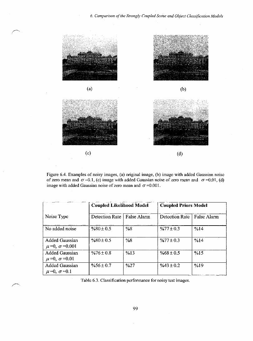
6. Comparison of the Strongly Coupled Scene and Object Classification Models
(a) (b)
(c) (d)
Figure 6.4. Examples ofnoisy images, (a) original image, (b) image with added Gaussian noise of zero mean and 0-=0.1, (c) image with added Gaussian noise of zero mean and 0-=0.01, (d) image with added Gaussian noise of zero mean and 0- =0.001.
Coupled Likelihood Model Cou pIed Priors Model
Noise Type Detection Rate FalseAlarm Detection Rate False Alann
No added noise %80±0.5 %8 %77±0.3 %14
Added Gaussian %80±0.5 %8 %77±0.3 %14 fi =0, 0- =0.001
Added Gaussian %76±0.8 %13 %68±0.5 %15 fi =0, 0- =0.01
Added Gaussian %56±0.7 %27 %43 ± 0.2 %19 fi =0, 0- =0.1
Table 6.3. Classification performance for noisy test images.
99
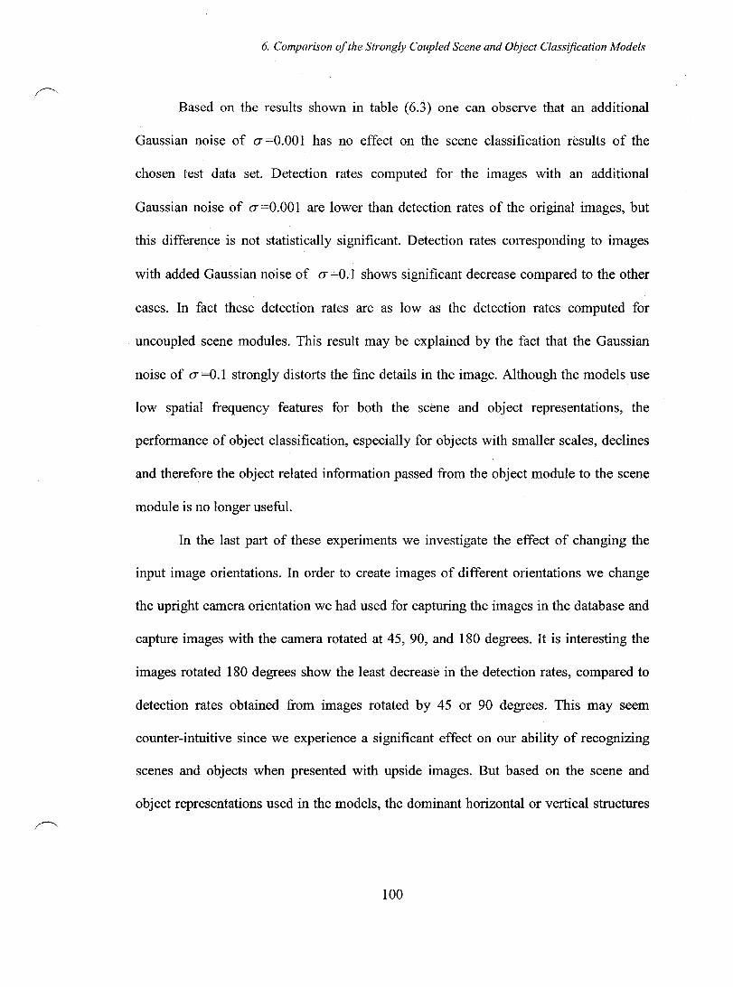
6. Comparison of the Strongly Coupled Scene and Object Classification Models
Based on the results shown in table (6.3) one can observe that an additional
Gaussian noise of (J" =0.001 has no effect on the scene classification results of the
chosen test data set. Detection rates computed for the images with an additional
Gaussian noise of (J" =0.001 are lower than detection rates of the original images, but
this difference is not statistically significant. Detection rates corresponding to images
with added Gaussian noise of (J" =0.1 shows significant decrease compared to the other
cases. In fact these detection rates are as low as the detection rates computed for
uncoupled scene modules. This result may be explained by the fact that the Gaussian
noise of (J" =0.1 strongly distorts the fine details in the image. Although the mode1s use
low spatial frequency features for both the scene and object representations, the
performance of object classification, especially for objects with smaller scales, declines
and therefore the object related information passed from the object module to the scene
module is no longer useful.
In the last part of these experiments we investigate the effect of changing the
input image orientations. In order to create images of different orientations we change
the upright camera orientation we had used for capturing the images in the database and
capture images with the camera rotated at 45, 90, and 180 degrees. It is interesting the
images rotated 180 degrees show the least decrease in the detection rates, compared to
detection rates obtained from images rotated by 45 or 90 degrees. This may seem
counter-intuitive since we experience a significant effect on our ability of recognizing
scenes and objects when presented with upside images. But based on the scene and
object representations used in the mode1s, the dominant horizontal or vertical structures
100
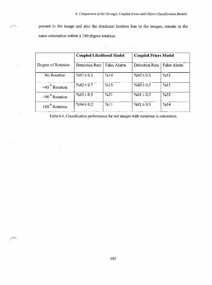
6. Comparison of the Strongly Cou pied Scene and Object Classification Models
present in the image and also the dominant horizon line in the images, remain in the
same orientation within a 180 degree rotation.
Cou pIed Likelihood Model Coupled Priors Model
Degree of Rotation Detection Rate False Alann Detection Rate FalseAlann
No Rotation %97±0.5 %14 %92±0.5 %15
+45 0 Rotation %82±0.7 %15 %86±0.3 %13
+900
Rotation %63±0.5 %21 %61 ± 0.2 %22
1800
Rotation %94±0.2 %11 %91±0.5 %14
Table 6.4. Classification performance for test images with variations in orientation.
101

~ ..
.~.
7. Attentional F eature Tuning
Chapter7
Attentional Feature Tuning
In the previous section we demonstrated the effect of the strong-coupling of the scene
and object modules on scene categorization results. The object classification and the
scene classification module make inferences about high-Ievel concrete (object) or
semantic (scene) concepts based on local or globallow level sensory features extracted
from the power spectrum of the images. The strongly-coupled feedback incorporated in
the model uses the inference made related to one of the high-Ievel concepts to influence
and adjust the inference made about the other high-Ievel concept. It is also possible to
create a top-down feedback between the high-Ievel inference processes and the lower
level feature extraction processes with the objective of creating an attention al
modulation effect which would make the scene or object classification process more
efficient. For example when the scene categorization module creates a hypothesis about
the identity of a scene based on the global features V G of the image, in the cases that the
identity of the image is ambiguous, meaning that the probability of the scene belonging
to two or more classes are smaller than a certain threshold, the feedback between the
object and the scene module may resolve this ambiguity based on evidence for presence
of object classes which can more clearly identify the scene. One other way of resolving
such ambiguity is to tune the features V G extracted from the scene image in order to
create higher discriminability between the ambiguous scene classes. In this chapter we
present the implementation and the experimental results of such a feature tuning scheme
102

r--..
7. Attentional Feature Tuning
where the hypothesis generated about the identity of the scenes is used to modify the
feature extraction process.
In the previous chapters we talked about the experiments by Oliva and Torralba
which show that the distribution of energy across the different scales and orientations of
the Gabor filter bank are stable enough among images belonging to the same scene
category, and therefore these distributions can be used as signatures representing the
scene classes [94]. In this chapter we propose using the energy distribution
characterizing each scene category to tune the Gabor filter bank used for producing the
low level features V G based on the scene hypothesis produced by the scene module. The
Bayesian inference function of the scene module represents the bottom-up flow of
infonnation in the model, where scene identities are inferred from the low level features
image features. The feature tuning represents the top-down flow of infonnation, where
the high-Ievel infonnation inferred from the scene identification module is used to tune
the low-Ievel features. This approach has conceptual similarity to the winner-take-all
model introduced by Tsotsos et al [97], but instead of the top-down winner-take-all
selection process biasing the features in sorne region of the image, representing the focus
of attention to that region, we use the hypothesis fonned by the scene module to bias
global image responses to selected spatial frequencies and orientations, therefore
attending to certain frequencies and orientations and not to a certain location in the
Image.
For this purpose we first study the energy levels of image responses to the Gabor
filter bank for images of different scene classes. We compute the average energy level of
the image responses from each scene c1ass to each Gabor filter (with specific orientation
103

~ ..
7. Attentional Feature Tuning
and sc ale ), and thus we create a "Gabor index" for each scene class. At the first iteration
of the model, the feature vector V G is extracted from the image without any a priori
hypothesis about the scene category, therefore the image responses to filters of different
scales and orientations are aIl used with equal weight for forming V G. But once the
probability of the image belonging to a scene class is estimated, this value can be used to
weight the image responses to different Gabor filters based on the corresponding "Gabor
Index". In this way we intend to enhance the image responses to filters with higher
energy levels and inhibit the image responses to filters with lower energy levels. The
newly formed V G is used in estimating the likelihoods PCV Gis j) for the next iteration.
We study the effect of combining the feature modulation and the feedback between the
object and the scene module on the scene classification performance.
7.1 Feature Tuning Scheme
In order to compute dominant power spectrum information for images belonging to each
scene class we use the total energy of the image responses to the bank of Gabor filters.
For a given image I(q,17) the image response to a Gabor filter tuned to radial frequency
f r and orientation B is given by
N V(x,y,fr,B)= "fJ(q,rJ)Gfr,(} (x-q,y-rJ)
;,1]=1
The total energy of the image response V (x, y, f r ,B ) is gi ven by
104
(7.1)
(7.2)
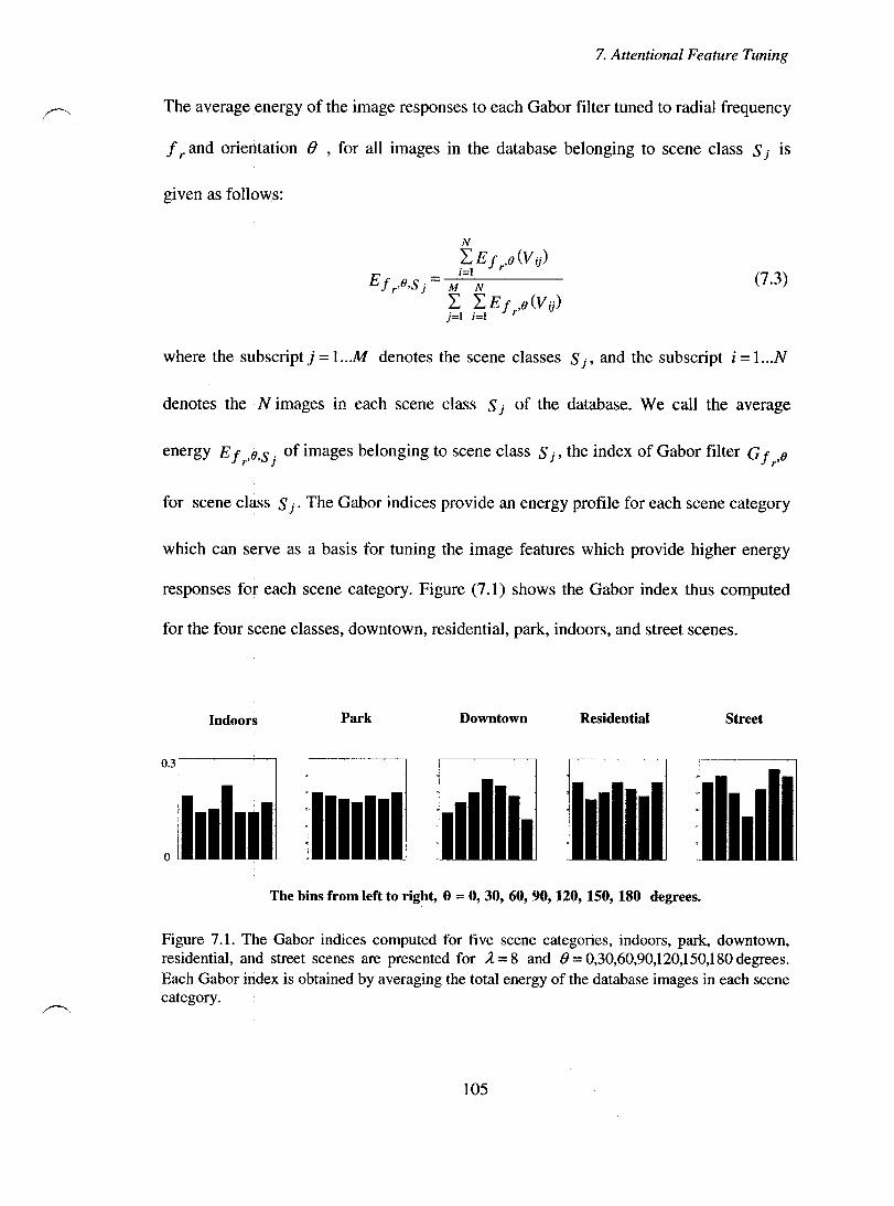
7. Attentional F eature Tuning
The average energy of the image responses to each Gabor filter tuned to radial frequency
f r and orientation 8 , for all images in the database belonging to scene class S j is
given as follows:
(7.3)
where the subscript j = 1 ... M den otes the scene classes S j' and the subscript i = 1 ... N
denotes the N images in each scene class S j of the database. We calI the average
energy E f r,e,S j of images belonging to scene class S j' the index of Gabor filter G f r,B
for scene class S j. The Gabor indices provide an energy profile for each scene category
which can serve as a basis for tuning the image features which provide higher energy
responses for each scene category. Figure (7.1) shows the Gabor index thus computed
for the four scene classes, downtown, residential, park, indoors, and street scenes.
Indoors Park Downtown Residential Street
0.3
o
The bins from left to right, 9 == 0, 30, 60, 90, 120, 150, 180 degrees.
Figure 7.1. The Gabor indices computed for tïve scene categories, indoors, park, downtown, residential, and street scenes are presented for  = 8 and 8 = 0,30,60,90,120,150,180 degrees. Each Gabor index is obtained by averaging the total energy of the database images in each scene category.
105

7. Attentional Feature Tuning
.~ .. Given an input image to the model, we can use the hypothesis formed by the scene
module to bias the image responses to selected Gabor filters which provide higher
discrimination for scene classes with higher probabilities. We weigh the image response
to a Gabor filter with radial frequency ! r and orientation fJ according to the probability
value of each scene class S j and index of the Gabor filter G f r,e for each scene class
S j as the following:
(7.4)
In each iteration of the model, in order to incorporate the top-down feature
tuning scheme based on the hypotheses created by the scene module, the modulated
image responses V (x, y,! r' fJ) are weighed based on the probability values estimated
for each of the scene classes at the previous iteration. The modulated image responses
V (x'Y'!r,fJ) replace V (x'Y'!r,fJ) for computing the global image features VG
used at the CUITent iteration of the model. Updating of the global image features V G ,
based on the modulated image responses, means. that- the likeliho0d--m0del estimations..
vary at each iteration of the model.
For the adaptive prior model the estimate of the likelihood P(V Gis j) vanes
based on the updated values of V G' and for the adaptive likelihood model the estimate
of the likelihood P(V G' P( 0 = 01)"", P( 0 = ON) 1 S j) varies not only based on the new
estimates for the object class probabilities, but also based on the new global image
features V G' As the model iterates, if one of the scene category probabilities computed
106

I~'
7. Attentional Feature Tuning
by the model dominates the other scene category probabilities, the corresponding Gabor
index gains more weight for the modulation of the image responses. In the next section
we show examples of how such a process affects the function of the scene classification
module, and in general the scene classification performance of the mode1.
7.2 Experimental ResuUs
Figures (7.2) and (7.3) present results of the model function when combined with feature
tuning effect as explained in the previous section. Figure (7.2) illustrates an ex ample of
the behavior of the coupled likelihoods model when combined with the feature tuning
effect and figure (7.3) illustrates an example of the behavior of the coupled priors model
when combined with the feature tuning effect.
The sample image in figure (7.2.a) IS a street scene. The probabilities of
buildings, plants, and vehicles being present in the scene, as computed by the coupled
likelihood model, without any feature tuning is shown in figure (7.2.b). The probabilities
of the image belonging to the scene categories street, park, downtown, and residential, as
computed by the coupled likelihood model, without feature tuning, is shown in figure
(7.2.c). Initially the mode1 computes close probability values for the image belonging to
the street category and the park category, but the object module finds more evidence for
vehicles being present in the image as compared to plants. The object probabilities
provide enough information for the scene module in order to gradually estimate higher
probabilities for the scene being a street scene. Figure (7.2.d) shows the probabilities of
this image belonging to the mentioned scene classes when the coupled likelihoods model
is combined with the feature tuning effect. Comparing figure (7.2.c) and (7.2.d) one can
107
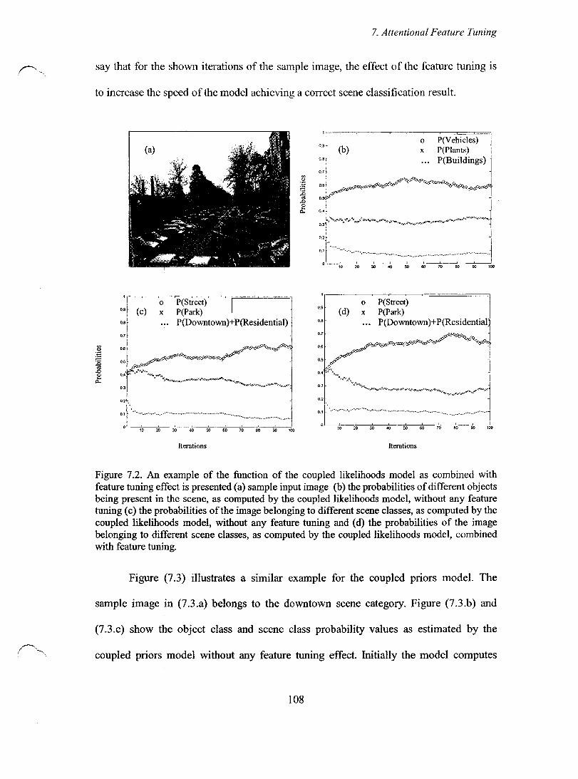
7. Attentional Feature Tuning
say that for the shown iterations of the sample image, the effect of the feature tuning is
to increase the speed of the model achieving a correct scene classification result.
0.9 (c)
02
o x
P(Street) 1 P(Park)
P(Downtown)+P(Residential)
0.1 ............................................................................................... .
Iterations
o P(VehicJes) (b) x P(Plants)
0.8 P(Buildings)
:'~-----j 0.4 ""'x.,., ...... x~)()(~i!'x,.-.x~~lOOt,.,.~>i><><.x __ " """""')<"x~)<,r...~;'o<)(0,i"'''>O<Y''',..''''><:><><'''''1 0.3 "><>'")0<"'-...... ,....,.,.,. 1 u J
0:···· .............................................................................. d
o.
• ~ ~ w ~ ~ ro 00 00 _
o (d) x
P(Street) P(Park) P(Downtown)+P(Residential
~ 1
o. ''''' .... ,.1'« "1 0.3 ~">o<">oI""><>Vl<)C><"'><X"""#"'''''''')(,<xl<'')(~'''''''",,>Qo)O<)'.,... ~-.?"'x")C<X''<'' 0.2 ''"~~"'<::::~< 'J 0.1 •••••••••••••••••••••••••••••••••••••••••••••••••••••••••••••••••••••••••••••••••••••••••••••
o -~~ • ~ ~ w ~ 00 ro 00 00 _
Iterations
Figure 7.2. An example of the function of the coupled likelihoods model as combined with feature tuning effect is presented (a) sample input image (b) the probabilities of different objects being present in the scene, as computed by the coupled likelihoods model, without any feature tuning (c) the probabilities of the image belonging to different scene classes, as computed by the coupled likelihoods model, without any feature tuning and (d) the probabilities of the image belonging to different scene classes, as computed by the coupled likelihoods model, combined with feature tuning.
Figure (7.3) illustrates a similar example for the coupled priors model. The
sample image in (7.3.a) belongs to the downtown scene category. Figure (7.3.b) and
(7.3.c) show the object class and scene class probability values as estimated by the
coupled priors model without any feature tuning effect. Initially the model computes
108
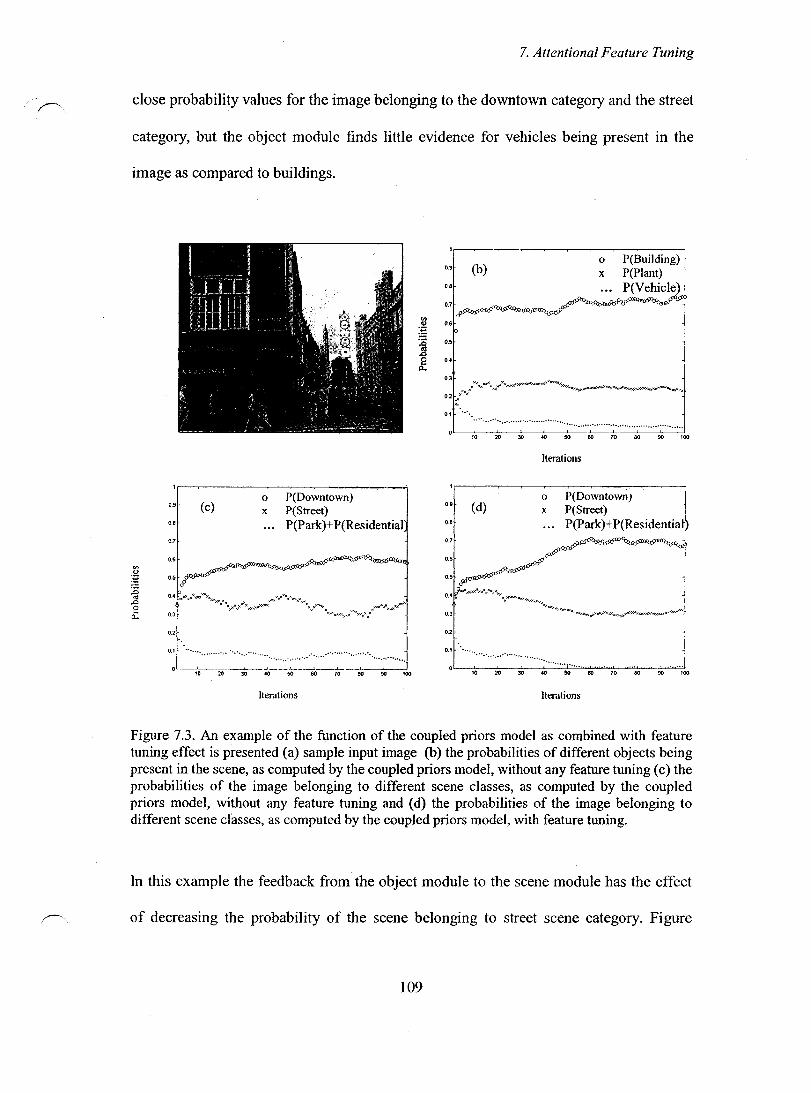
.~.
7. Attentional Feature Tuning
close probability values for the image belonging to the downtown category and the street
category, but the object module finds little evidence for vehicles being present in the
image as compared to buildings.
0.9 (c) o P(Downtown) x P(Street)
o .• P(Park)+ P(Residential 0.7
o .•
02
0.1 •••••••••••••••••••••••••••••••••.•••••••••••••••••••••••••••••••••••••••.•••••••••••••••••••••
o ._.L __ ......... ___ . ..L~ __ .• .J.. __ ._.L...._ .. --1_. __ ..l._._.--l._
g ~ ~ ~ ~ ~ n ro 00 m
Iterations
0.9 (b) o P(Bui)ding) x P(Plant)
o.. ••• P(Vehicle) 0.7 ""'~_. ~ooxY'O' _,~M 6'~-~~=»<)~ .
o .• p
0.5
o.,
0.1 •••• ..................................... ........................ .................. .
0,9 (d) o .•
0.7
Iterations
o x
P(DowntoWll) ) P(Street) P(Park)+ p(Residentia~
o.. ~../' O.5~"'--
0.2
0.1 •••••••••••••• _
. ........... . 10 20 30 ~ 70 80 100
Iterations
Figure 7.3. An example of the function of the coupled priors model as combined with feature tuning effect is presented (a) sample input image (b) the probabilities of different objects being present in the scene, as computed by the coupled priors model, without any feature tuning (c) the probabilities of the image belonging to different scene classes, as computed by the coupled priors model, without any feature tuning and (d) the probabilities of the image belonging to different scene classes, as computed by the coupled priors model, with feature tuning.
In this example the feedback from the object module to the scene module has the effect
of decreasing the probability of the scene belonging to street scene category. Figure
109

r---..
7. Attentional Feature Tuning
(7.3.d) shows the behavior of the model when the coupling of the priors is combined
with the feature tuning effect. Similar to the ex ample above the effect of feature tuning
for this sample image is that the model achieves higher probabilities for the correct
scene class identity in earlier iterations.
Examples in the previous two figures have been selected among experimental
results in order to illustrate the capability of the feature tuning to increase the scene
classification performance. In order to make a statistically valid conclusion about the
effect of feature tuning on the scene classification performance we plot ROC curves.
Figure (7.4) and (7.5) contain the receiver operating characteristic (ROC) curves for
scene classification task performed by the coupled priors and coupled likelihoods
models when their functionality is combined with the feature tuning effect. In figures
(7.4) and (7.5) each curve represents results from varying decision thresholds of a fixed
iteration of the model. Comparing the curves representing performance at the first and
the l00th iteration of the two models we can see that classification performance is higher
at the 100th iteration in both models. It is also important to compare the performances of
the two models with feature tuning with the performances of the two models without any
feature tuning. Therefore, we have included relevant plots in figures (7.4) and (7.5) to
make the comparisons easier. One can observe that the models with feature tuning
achieve higher classification performance at the 100th iteration as compared to the
models without feature tuning. In general one can conclude that the effect of combining
feature tuning with the strongly coupled models is that on average a higher detection rate
is achieved with fewer iterations, at least within the first 100 iterations of the model.
110
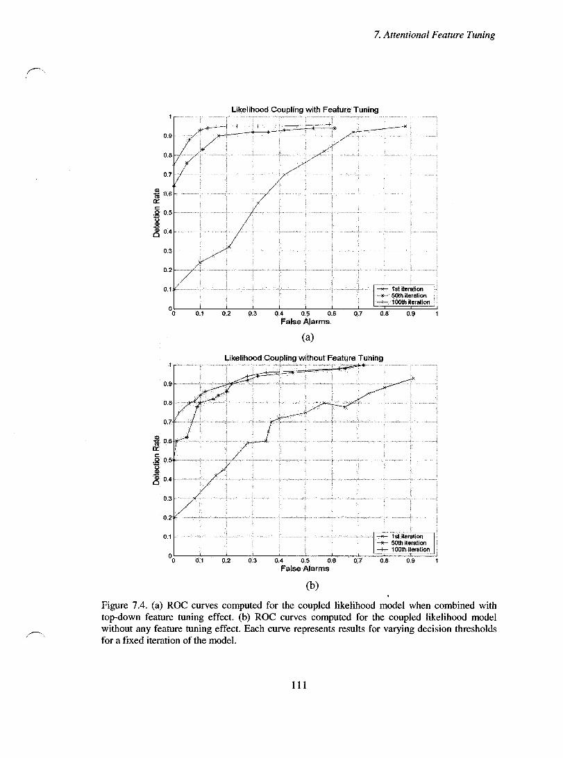
7. Attentional Feature Tuning
Likelihood Coupling with Feature Tuning
0.9
0.8
0.7
"* 0.6 n:: s::::
.Q 0.5 1) CI)
~ 0.4
0.3
0.2 ..
0.1
0 0 0.1
(a)
(b)
Figure 7.4. (a) ROC curves computed for the coupled likelihood model when combined with top-down feature tuning effect. (b) ROC curves computed for the coupled likelihood model without any feature tuning effect. Each curve represents results for varying decision thresholds for a fixed iteration of the model.
111
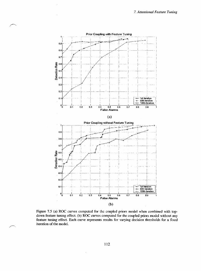
7. Attentional Feature Tuning
Prior Coupling with Feature Tuning
Ca) Prior Coupling without Feature Tuning
0.8 ........ .1.. .... 0 ••• , .... J ...
o.
0.1
°0L---~--~~--~--~~--~--~~--~~=?~~~~=J 0.4 0.5 0.6 0.9
False Alarms
Cb)
Figure 7.5 (a) ROC curves computed for the coup1ed priors mode1 when combined with topdown feature tuning effect. (b) ROC curves computed for the coup1ed priors mode1 without any feature tuning effect. Each curve represents results for varying decision thresho1ds for a fixed iteration of the model.
112

8. Conclusions and Future Work
Chapter 8
Conclusions and Future W ork
8.1 Conclusions
In this thesis, we have presented a strongly coupled data fusion architecture within a
Bayesian framework that mode1s the associations between the scene and object
classification mechanisms. Based on findings from the domains of neurophysiology and
psychophysics there is adequate experimental evidence to suggest that the scene
perception mechanism and the object perception mechanism in hum an vision do not
function in isolation. There is experimental evidence which shows that scene-contextual
constraints are available early enough and are robust enough to influence the object
recognition mechanism, also rapid recognition of familiar objects influences the scene
recognition mechanism. These experimental results imply the presence of a bidirectional
flow of information between the scene and the object recognition mechanisms, while
contradicting a strictly hierarchical relationship between the two processes in any order.
These findings have motivated us to develop an architecture that can give a
computational account of how such a relationship is possible between the object
classification and the scene classification processes. The most important characteristic of
the architecture proposed in this thesis is that it avoids a hierarchical relationship
between the two processes, so that each of the processes can function independently in
case of lack of feedback from the other process. A feedback channel is provided between
the two processes so that as soon as any of the two processes extracts any information
113

8. Cone/usions and Future Work
about the identity of the scene or the identity of the objects present in the scene, this
information becomes available to the other process.
Our proposed architecture is derived from Clark and Yuille's [14] work. In their
work they present a general architecture for strongly-coupled data fusion of separate
sensory information processing modules, with the purpose of regularizing the ill-posed
problem involved with each sensory information processing task. We have used this
general structure and have adapted it to the specific problem of the strong coupling of
two modules which are specialized in the scene classification and the object
classification tasks. The strong coupling of the two modules provide additional
constraints for each module's solution process based on the information obtained from
the independent process of the other module. The Bayesian approach taken for solving
the tasks assigned to each module has the advantage of providing a suitable form for
embedding constraints either in the likelihood models or the prior models of the
modules' solution processes. In this thesis we have presented novel schemes for
modifying the Bayesian solutions for the scene and object classification tasks which
allow data fusion between the two modules based on the constraining of the priors or the
likelihoods.
We have implemented the two proposed models and tested the model functions
usmg a data base of natural images created for this purpose. We have presented
examples of the model outputs for images of different scene categories which illustrate
how the feedback between the two modules can improve the initial scene classification
results obtained from the uncoupled scene module. The ROC curves plotted for the
likelihood coupling and the prior coupling mode1s show that the scene classification
114

8. Cone/usions and Future Work
perfonnance improves significantly in both models as a result of the strong coupling of
the scene and object modules. The shapes of the autocorrelation plots obtained from both
models' outputs demonstrate the predictability of the two models' processes. We have
also tested the robustness of the two models to variations to the input test images such as
added noise. ROC curves depicting the scene classification perfonnance of the two
models also show that the likelihood coupling model achieves a higher detection rate
compared to the prior coupling model. We have also computed the average rise times of
the models' outputs as a measure of comparing the speed of the two models. The results
show that the likelihood coupling model outputs have a shorter rise time. Based on these
experimental findings one can conclude that imposing constrains on the likelihood
models provide better solutions to the scene classification problems compared to
imposing constraints on the prior models. This result is compatible with the general
concept that the prior models represent smoother functions compared to the likelihood
models. Imposing constraints on the likelihood models, which are more sensitive
functions compared to the prior models, improves the Bayesian solution more than
imposing constraints on prior models, which are smoother, slower varying functions.
We have also proposed an attentional feature modulation scheme, which consists
of tuning the input image responses to the bank of Gabor filters based on the scene class
probabilities estimated by the model and the energy profiles of the Gabor filters for
different scene categories. Experimental results based on combining the attentional
feature tuning scheme with the likelihood coupling and the prior coupling methods show
a significant improvement in the scene classification perfonnances ofboth models.
115

8. Conclusions and Future Work
The question of coupling the object classification process and the scene
classification process has been addressed by other researchers in the field of machine
leaming such as Murphy et al [65]. The approach taken by these researchers is to
combine the tasks of scene classification and object presence detection using a tree
structural graphical model, where the message passing runs first bottom-up (objects to
scenes) and then top-down (scenes to objects). The graphical model encodes a
conditional joint probability density model of the scene class and the object classes
present in the scene as constrained by the global contextual features. Our approach to
combining the scene classification and the object classification tasks differ from this
approach in a fundamental way. Our main goal in developing the proposed architecture
was its biological relevance, and not necessarily building a model for efficient scene or
object classification. Therefore, we imposed certain constraints to our model, such as
avoiding a hierarchical relationship between the object and scene classification modules,
in order to develop a computational scheme which would explain the relationship
between the scene and object recognition process in human visual system based on
psychophysical findings.
8.2 Future Work
Our main challenge in developing a model where the scene processing and the object
processing modules would interact, was to find a way to combine results from local and
global sources of information. There are three types of local information produced by the
object processing module, the identity of the objects, the location of the objects, and the
scale of the objects. In the present implementation of the model the local information
116

8. Conclusions and Future Work
extracted about the identities of the objects are combined with each other and interact
with the global source of information, but we make no use of the objects' locations and
scales, while both the scales of the objects and their locations provide strong constraints
for the scene classification problem. Therefore, the proposed model can be enhanced by
modifying the present formulation in order to include scales and locations of the objects
as part of the information passed between the modules.
Our present method of identifying objects in a scene is based on sliding a
detector over the whole scene and classifying the patches at each location and scale. We
can improve the speed and the accuracy of our object classification module by reducing
the search space for objects. This can be implemented either by using prior constraints
from the scene classes inferred from the scene classification module. Scene classes
provide strong constraints on the locations where certain object classes may be found.
We can also reduce the search space for the objects by using an attentional scheme
which would highlight the most conspicuous locations of the scene. This may provide a
way to reduce the amount of irrelevant information processed and to focus on the most
informative or the most interesting locations of the scene. Such a scheme would also be
closer to how humans fixate on different locations in a scene, rather than covering the
whole scene with a pre-assigned order.
What we consider a very challenging and interesting issue to be addressed in
future work is the issue of moving from a highly supervised model, such as the model
presented in this thesis, to an unsupervised model, where new scene and object
categories can be leamed from the data. Also the choice of levels of abstractions for
scene and object classes in a supervised model is a challenging decision. While
117

8. Cane/usions and Future Work
designing the experiments for the implementation of our model we had to deal with the
problem of choosing appropriate levels of abstraction for the scene and object categories,
in order to allow useful information being produced for the use of the other model.
Changing the levels of abstraction from basic level categories such as the ones we have
used in our experiments to more general or finer discrimination categories may involve
modifications to the proposed model which has to be investigated further.
118
r~ References
[1] G. K. Agui rre. , "The parahippocampus subserves topographical leaming in man," Cortex, vol. 6, pp. 823-829, 1996.
[2] R. Baddeley, "The correlational structure of natural images and the calibration of spatial representations," Cogn. Sci. vol. 21, pp. 351-372, 1997.
[3] M. Bar and S. Ullman, "Spatial context in recognition," Perception, vol. 25, pp.343-352, 1996.
[4] M. Bar and E. Aminoff, "Cortical analysis of visual context," Neuron vol. 38, pp. 347-358,2003.
[5] 1. Biederman, "Perceiving real-worId scenes," Science, vol. 177, pp. 77-80, 1972.
[6] 1. Biederman, "On the semantics of a glance at a scene," Perceptual Organization, pp. 213-254, 1981.
[7] 1. Biederman, R. C. Teitelbaum, and R. J. Mezzanotte, "Scene perception: a failure to find a benefit from prior expectancy or familiarty," J. of Exp. Psychol., vol. 9(3), pp. 411-429, 1983.
[8] 1. Biederman, "Recognition-by-Components: A theory of human image understanding," Psychological Review, vol. 94, pp. 115-147,
[9] S. J. Boyce, A. Pollatsek, and K. Rayner, "Effect of background information on object identification," J. Exp. Psycho!. Hum. Perc. and Perf, vol. 15(3), pp. 556-566, 1989.
[10] L. Breiman, "Bagging predictors," Machine Learning, vol. 26(2), pp. 123-140, 1996.
[11] J. Bullier and L. G. Nowak, "ParaIlei versus seriaI processing: new vistas on the distributed organization ofthe visual system," Curr. Opin. Neurobiol.vol. 5, pp. 497-503 1995.
[12] M. BurI and P. Perona, "Recognition of planar object classes," Proc .of Computer Vision and Pattern Recognition, pp. 223-230, 1996.
[13] S. Belongie, C. Carson, H. Greenspan, and J. Malik, "Color and texture based image segmentation using EM and its application to image querying and classification," Proc. of the Int. Conf Computer Vision, pp. 675-672, 1998.
119
[14] J. 1. Clark and A. L. Yuille," Data Fusion for Sensory Information Processing Systems, USA: Kluwer Academic Publishers, 1990.
[15] B. V. Dasarthy, Decision Fusion, Los Alamitos, CA: IEEE Computer Society Press.
[16] P. De Graef, D. Christiaens, and G. d'Ydewalle, "Perceptual effects of scene context on object identification," Psychol. Res., vol. 52, pp. 317-329, 1990.
[17] P. E. Downing., "A cortical area selective for visual processing of the human body," Science vol. 293, pp. 2470-2473,2001.
[18] T. Ehtiati and J. J. Clark, "A Bayesian Model for the Bi-directional Influences between the Scene and the Object Identification Processes", Proc. of the International Workshop on the Representation and Use of Prior Knowledge in Vision (WRUPKV), in association with the 9th European Conference on Computer Vision (ECCV), pp. 126-139,2006.
[19] T. Ehtiati and J. J. Clark, "A Strongly Coupled Architecture for Contextual Object and Scene Identification", Proc. of the 1 i h IEEE International Conference on Pattern Recognition (ICPR), vol. 3, pp. 69-72, 2004.
[20] R. A. Epstein, "The cortical basis ofvisual scene processing," Visual Cogn, vol. 12, pp. 954-978, 2005.
[21] R. Epstein and N. Kanwisher, "A cortical representation of the local vi suaI environment," Nature, vol. 392, pp. 598-601, 1998.
[22] L. Fei-Fei, R. Fergus, and P. Perona, "Leaming generative visual models from few training examples: an incremental Bayesian approach tested on 101 object categories," Workshop on Generative-Model Based Vision, 2004 (in press).
[23] L. Fei-Fei, R. VanRullen, C. Koch, and P. Perona, "Rapid natural scene categorization in the near absence of attention," Proc. Nat. Acad. Sci., vol. 99(14), pp. 9596-9601,2002.
[24] L. Fei-Fei, R. Fergus, and P. Perona, "A Bayesian approach to unsupervised oneShot learning of object categories," Proc. of Int. Conf on Computer Vision, pp. 1134-1141,2003.
[25] L. Fei-Fei, R. Fergus, and P. Perona, "One-Shot leaming of object categories," IEEE Trans. on Pattern Analysis and Machine Intelligence, vol. 28(4), pp. 594-611, 2006.
[26] R. Fergus, P. Perona, and A. Zisserman, "Object c1ass recognition by unsupervised scale-invariant leaming," Proc. of Computer Vision and Pattern Recognition, pp. 264-271,2003.
120
[27] M. Flickner and H. Sawhney, "Query by image and video content: The QIBC system," IEEE Computer, vol. 28(9), pp. 23-32, 1995.
[28] Y. Freund and R. E. Schapire, "Experiments with a new boosting algorithm, " Proc. of the Thirteenth Int. Conf on Machine Learning, pp. 148-156, 1996.
[29] Y. Freund and R. Schapire, "A short introduction to boosting," Journal of Japanese Society for ArtificialIntelligence, vol. 14(5), pp. 771-780, 1999.
[30] A. Friedman, "Frame pictures: the role of knowledge in automatized en co ding and memory for gist," J. of Exp. Psycho!. General, vol. 108(3), pp.316-355, 1979.
[31] J. D. Gabrieli, R. A. Poldrack, and J. E. Desmond, "The role of left prefrontal cortex in language and memory," Proc. Nat! Acad. Sci. USA, vol. 95, pp.906-913, 1998.
[32] A. Gelb, Applied Optimal Estimation. Cambridge, MA: MIT Press 1974.
[33] F. Germeys and G. d'Y dewalle, "Revisiting scene primes for object locations," Quart. J. Exp. Psychol., vol. 54A(3), pp. 683-693,2001.
[34] M. Gorkani and R. W. Picard, "Texture orientation for sorting photos at a glance," Proc. of the Int. Conf on Pattern Recognition, vol. 1, pp. 459-464, 1994.
[35] C. V. Gottesman and H. Intraub, "Wide-angle memories of close-up scenes: a demonstration of boundary extension,", Behav. Res. Methods Instrum. Comp., vol. 31(1), pp. 86-93, 1999.
[36] K. Grill-Spector, Z. Kourtzi, and N. Kanwisher, "The lateral occipital complex and its role in object recognition," Vision Res., vol. 41, pp. 1409-1422,2001.
[37] K. Grill-Spector and N. Kanwisher, "Visual recognition: as soon as you know it is there, you know what it is," Psychol. Sci., vol. 16 (2) ,pp. 152-160,2005.
[38] A. Gupta and R. Jian, "Visual information retrieval," Communications of the A CM, vol. 40(5), pp. 71-79, 1997.
[39] J. V. Haxby, "Distributed and overlapping representations of faces and objects in ventral temporal cortex," Science, vol. 293, pp. 2425-2430, 2001.
[40] J. M. Henderson and A. Hollingworth, "High-level scene perception," Annu. Rev. Psychol., vol. 50, pp. 243-271, 1999.
[41] A. Hollingworth and J. M. Henderson, "Object identification is isolated from scene semantic constraint: evidence from object type and token discrimination," Acta Psychol (Amst), vol. 102(2-3), pp. 319-343, 1999.
121
[42] J. Huang, S. R. Kumar, and R. Zabih, "An automatic hierarchical image classification scheme," Proc. of Sixth A CM Inti. Multimedia Conf., pp. 219-228, 1998.
[43] Y. S. Huang and C. y. Suen, "A method of combining multiple experts for recognition of unconstrained handwritten numerals," IEEE Trans. on Pattern Analysis and Machine Intelligence, vol. 17 (1), pp.90-94, 1995.
[44] D. H. Hubel and T. N. Wiesel, "Receptive fields and functional architecture of the monkey striate cortex," Journal of Physiology, vol. 195, pp.215-243, 1968.
[45] D. HubeI and T. Wiesel, " Binocular interaction and functional architecture in the catIs visual cortex," Journal of Physiology, vol. 160, pp. 106-154, 1962.
[46] H. Intraub, "Boundary extension for briefly glimpsed photographs: do common perceptual pro cesses result in unexpected memory distortions?" J. Mem. Lang., vol. 35, pp. 118-134, 1996.
[47] R. A. Jacobs, M. 1. Jordan, S. J. Nowlan, and G. E. Hinton, "Adaptive mixtures of local experts," Neural Computation, vol. 3, pp. 79-87, 1991.
[48] M. 1. Jordan and R. A. Jacobs, "Hierarchical mixtures of experts and the EM algorithm," Neural Computation, vol. 6, pp. 181-214, 1994.
[49] J. Kittler, M. Hatef, R. P. W. Duin, and J. Matas, "On combining classifiers," IEEE Trans. on Pattern Analysis and Machine Intelligence, vol. 20(3), pp. 226-239, 1998.
[50] S. M. Kosslyn, R. A. Flynn, J. B. Amsterdam, and G. Wang, "Components ofhighlevel vision: A cognitive neuroscience analysis and accounts of neurological syndromes," Cognition, vol. 34, pp. 203-277, 1990.
[51] L. Lam and C. Y. Suen, "Optimal combinations of pattern classifiers," Pattern Recognition letters, vol. 16, pp. 945-954, 1995.
[52] Y. LeCun, L. Bottou, Y. Bengio, and P. Haffner, "Gradient-based leaming applied to document recognition," Proc. of the IEEE, vol. 86(11), pp. 2278-2324, 1998.
[53] T. Leung, M. Burl, and P. Perona, "Finding faces in cluttered scenes using labeled random graph matching," Proc. Int. Conf on Computer Vision, pp. 637-644, 1995.
[54] 1. Levy, "Center-periphery organization ofhuman object areas," Nature Neurosci., vol. 4, pp. 533-539, 2001.
[55] P. Lipson, "Context and Configuration Based Scene Classification," EECS dept, PhD thesis MIT, 1996.
122
[56] G. R. Loftus, W. W. Nelson, and H. J. Kallman, "DifferentiaI acquisition rates for different types of information from pictures," Q. J. Exp. Psychol. vol. 35A, pp. 187-198, 1983.
[57] E. A. Maguire., "Knowing where things are: parahippocampal involvement in encoding object locations in virtual large-scale space," J. Cogn. Neurosci., vol. 10, pp. 61-76, 1998.
[58] J. M. Mandler and R. E. Parker, "Memory for descriptive and spatial information in complex pictures," J. of Exp. Psychol., vol. 2(1), pp. 38-48, 1976.
[59] D. Marr, Vision, USA: W.H. Freeman, 1981.
[60] G. J. McLachlan and T. Krisshnan, The EM Algorithm and Extenstions, USA: John Wiley & Sons Inc. 1997.
[61] W. H. Merigan and J. H. Maunsell, "How parallel are the primate visual pathways?" Annu. Rev. Neuroscie., vol. 16, pp. 369-402, 1993.
[62] R. L. Metzger and J. R. Antes, "The nature of processing early lU picture perception," Psychol. Res., vol. 45, pp. 267-274, 1983.
[63] T. P. Minka and R. W. Picard, "Interactive learning using a society of models," Proc. ofCVPR IEEE Computer Society, pp. 447-452, 1996.
[64] M. Mishkin, L. G. Ungerleider, and K. A. Macko, "Object vision and spatial vision: Two cortical pathways," Trends Neurosci., vol. 6, pp. 414-417, 1983.
[65] K. Murphy, A. Torralba, and W. Freeman, "Using the forest to see the trees: a graphical model relating features, objects and scenes," Neural info. Processing Systems, Vancouver, B.C., 2004.
[66] A. Oliva and P. G. Schyns, "Coarse blobs or fine edges? Evidence that information diagnosticity changes the perception of complex visual stimuli," Cognitive Psychology, vol. 34, pp. 72-107, 1997.
[67] A. Oliva and P. G. Schyns, "Colored diagnostic blobs mediate scene recognition," Cognitive Psychology, vol. 41, pp.176-210, 2000.
[68] A. Oliva and A. Torralba, "Modeling the shape of the scene: a holistic representation of the spatial Envelope," Int. Journal of Computer Vision, vol. 42(3), pp. 145-175,2001.
[69] A. Oliva and A. Torralba, "Scene-Centered Description from Spatial Envelope Properties," Proc. 2nd Workshop on Biologically Motivated Computer Vision, Tubingen, Germany, 2002.
123
[70] A. Oliva, A. Torralba, A. Guerin-Dugue, and J. Herault, "Global semantic classification of scenes using power spectrum templates," Proe. of The Challenge of Image Retrieval. Electronic Workshop Computer Series, Springer-Verlag, 1999.
[71] A. Oliva, "Gist of a Scene," Neurobiology of Attention, Academic Press, Elsevier pp. 251-256.
[72] J. K. O'Regan and A. Noë, "What it is like to see: A sensorimotor theory of visual experience," Synthese, vol. 129(1), pp. 79-103, 2001.
l73] J. K. O'Regan, R. A. Rensink, and J. J. Clark, "Blindness to scene changes caused by "mudsplashes"," Nature, vol. 398, pp. 34, 1999.
[74] S. E. Palmer, "Visual perception and world knowledge: notes on a mode1 of sensory-cognitive interaction," Explorations in Cognition, pp. 279-307. LNR Res. Group, San Francisco, 1975.
[75] T. Poggio and S. Edelman, "A network that leams to recognize 3D objects," ,Nature vol. 343, pp. 263-266, 1990.
[76] M. C. Potter, "Short-terrn conceptual memory for pictures," J of Exp. Psychol. Hum. Learning and Mem, vol. 2, pp. 509-522, 1976.
[77] M. C. Potter, A. Staub, J. Rado, and D.H. O'Connor, "Recognition memory for briefly presented pictures: the time course of rapid forgetting," J Exp. Psychol: Hum. Pere. and Perl, vol. 28(5), pp. 1163-1175,2002.
[78] A. Puce, T. Allison, M. Asgari, J. C. Gore, and G. McCarthy, "DifferentiaI sensitivity of human visual cortex to faces, letterstrings, and textures: a functional magnetic resonance imaging study," J Neurosci., vol. 16, pp. 5205-5215, 1996.
[79] A. L. Ratan and W. E. L. Grimson, "Training ternplates for scene classification using a few exarnples," Proc. of IEEE Workshop on Content-Based Access of Image and Video Libraries, pp. 90-97, 1997.
[80] R. A. Rensink, J. K. O'Regan, and J. J. Clark, "To see or not to see: the need for attention to perceive changes in scenes," Psychol. Sei., vol. 8(5), pp. 368-373, 1997.
[81] G. Rousselet, M. Fabre-Thorpe, and S. Thorpe, "Paralle1 processing in high-1eve1 categorization of natural images," Nature Neuroseience, vol. 5, pp. 629-630, 2002.
[82] H. Rowley, S. Baluja, and T. Kanade, "Neural network-based face detection," IEEE Trans. On Pattern Analysis and Machine Intelligence., vol. 20(1), pp. 23-38, 1998.
[83] A. M. Schmid and M. Bar, "Activation of multiple candidate object representations during top-down facilitation of visual recognition," Soc. Neurosei. Abstr. vol. 128(5), 2003.
124
[84] H. Schneidennan and T. Kanade, "A statistical approach to 3D object detection applied to faces and cars," Proc. of Computer Vision and Pattern Recognition, pp. 746-751,2000.
[85] J. R. Smith and S. F. Chang. "Visualseek: A fully automated content-based image query system," ACM Multimedia, pp. 87-98, 1996.
[86] L. Standing, "Leaming 10,000 pictures," Quarterly Journal of Experimental Psychology, vol. 25, pp. 207-222, 1973.
[87] L. Standing, J. Conezio, and R. N. Haber, "Perception and memory for pictures: Single-trial leaming of 2,500 visual stimuli," Psychonomic Science, vol. 19, pp. 73-74, 1970.
[88] C. E. Stem, "The hippocampal fonnation participates in noveI picture encoding: evidence from functional magnetic resonance imaging," Proc. Nat! Acad. Sci., vol. 93, pp. 8660-8665, 1996.
[89] K. Sung and T. Poggio, "Example-based leaming for view-based human face detection," IEEE Trans. on Pattern Analysis and Machine Intelligence, vol. 20(1), pp. 39-51, 1998.
[90] M. Szummer and R. Picard, "1ndoor-outdoor image classification," Int. Workshop on Content-based Access of Image and Video Databases, 1998.
[91] K. Tanaka, "Neuronal mechanisms of object recognition," Science, vol. 262, pp. 685-688, 1993.
[92] M. Tarr and H. Bulthoff, "1s human object recognition better described by geon structural descriptions or by multiple views? Comment on Biederrnan and Gerhardstein (1993)," J. Exp. Psycho!. Hum. Percept. Perform, vol. 21, pp. 1494-1505, 1995.
[93] S. Thorpe, D. Fize, and C. Marlot, "Speed of processing in the hurnan visual system," Nature, vol. 381, pp. 520-522, 1996.
[94] A. Torralba and A. Oliva., "Statistics of natural image categories," Network: computation in neural systems. vol. 14, pp.391-412, 2003.
[95] A. Torralba and A. Oliva, "Depth estimation from image structure," IEEE Trans. on Pattern Analysis and Machine Intelligence, vol. 24(9), pp. 1226-1238, 2002.
[96] A. Treisman and G. Gelade, "A feature-integration theory of attention," Cogn. Psychol., vol. 12, pp. 97-136, 1980.
125
[97] J. K. Tsotsos, S. Culhane, W. Wai, y. Lai, N. Davis, and F. Nuflo, "Modeling visual attention via selective tuning," Artificial Intelligence, vol. 78(1-2), pp. 507-547, 1995.
[98] L. G. Ungerleider and M. Mishkin, "Two cortical visual systems," Analysis of Visual Behavior, pp. 549-586, MIT press, Cambridge, Mass., 1982.
[99] A. Vailaya, M. Figueiredo, A. Jain, and H. Zhang, "Image classification for content-based indexing," IEEE Trans. on Image Processing, vol. 10, 2001.
[100] A. Vailaya, M. Figueiredo, A. Jain, and H. Zhang, "A Bayesian Framework for Semantic Classification of Outdoor Vacation Images," Proc. of SPIE Conference on Electronic Imaging, San Jose, California, 1999.
[101] D. C. Van Essen, "Functional organization of primate visual cortex," Cerebral Cortex, vol. 3, pp. 259-329. Plenum Press, 1985.
[102] P. K. Varshney, Distributed Detection and Data Fusion, New York: Springer Verlag, 1997.
[103] P. Viola and M. Jones, "Rapid object detection using a boosted cascade of simple features," Proc. of Computer Vision and Pattern Recognition, vol. 1, pp. 511-518,2001.
[104] P. Viola, M. Jones, and D. Snow, "Detecting pedestrians using patterns ofmotion and appearance," Proc. of the Int. Conf on Computer Vision, pp. 734-741, 2003.
[l05] E. Waltz and J. Llinas, Multisensor Data Fusion, Boston: Artech Rouse, 1990.
rl06] M. Weber, M. Welling, and P. Perona, "Unsupervised leaming of models for recognition," Proc. of the European Conf on Computer Vision, vol. 2, pp. 101-108, 2000.
[107] J. M. Wolfe, "Visual search," Attention, pp. 13-74, Psychology Press Ltd., 1998.
[108] J. M. Wolfe, "Visual memory: what do you know about what you saw?" Curr. Bio, vol. 8, pp. R303-R304, 1998.
[109] K. Woods, W. P. Kegelmeyer, and K. Bowyer, "Combination of multiple classifiers using local accuracy estimates," IEEE Trans. on Pattern Analysis and Machine Intelligence, vol. 19, pp. 405-410, 1997.
[110] E. C. Yiu, "Image classification using color eues and texture orientation," dept. EECS, Masters's thesis MIT, 1996.
[111] H. Yu and W. Wolf, "Scenic classification methods for image and video databases," Proc. SPIE, Digital Image Storage and Archiving Systems, pp. 363-371, 1995.
126

[112] H. J. Zhang and D. Zhong, "A scheme for visual feature based image indexing," Proc. SPIE Conference on Storage and Retreival for Image and Video da ta bases , San Jose, CA, pp. 36-46, 1995.
[113] D. Zhong, H. J. Zhang, and S. F. Chang, "Clustering methods for video browsing and annotation," Proc. SPIE Conference on Storage and Retreival for Image and Video databases, San Jose, CA, 1995.
127