scattering amplitudes - international centre for...
TRANSCRIPT
ICTP Summer School, June 2017
Scattering Amplitudes LECTURE 2
Jaroslav TrnkaCenter for Quantum Mathematics and Physics (QMAP), UC Davis

Review of Lecture 1

Spinor helicity variables
✤ Standard SO(3,1) notation for momentum
✤ Matrix representation
pµ = (p0, p1, p2, p3)
pab = �µabpµ =
✓p0 + ip1 p2 + p3p2 � p3 p0 � ip1
◆
On-shell: p2 = det(pab) = 0
Rank (pab) = 1
pj 2 Rp2 = p20 + p21 + p22 � p23

Spinor helicity variables
✤ Rewrite the four component momentum
✤ Little group scaling
✤ Invariants
pµ1 = �µaa �1a
e�1a
h12i ⌘ ✏ab�1a�2b [12] ⌘ ✏abe�1a
e�2b
s12 = h12i[12]
� ! t�
e� ! 1
te�
p ! p

Three point amplitudes
✤ Three point kinematics
✤ Two solutions:
p21 = p22 = p23 = 0 p1 + p2 + p3 = 0
h12i = h23i = h13i = 0
�1 ⇠ �2 ⇠ �3
[12] = [23] = [13] = 0
e�1 ⇠ e�2 ⇠ e�3
No solution for real momenta (��+)(+ +�)
spin-S amplitudesE.g.✓
[12]3
[23][31]
◆S ✓h12i3
h23ih31i
◆S
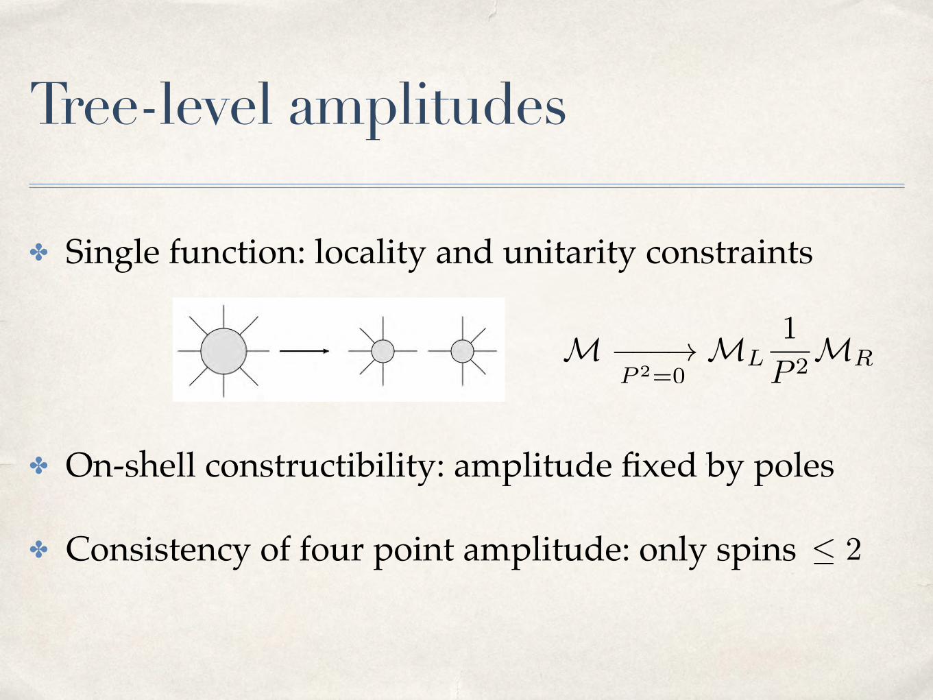
Tree-level amplitudes
✤ Single function: locality and unitarity constraints
✤ On-shell constructibility: amplitude fixed by poles
✤ Consistency of four point amplitude: only spins
M ���!P 2=0
ML1
P 2MR
2
Recursion relations

Tree level amplitudes
✤ Tree-level amplitude is a rational function of kinematics
✤ Only poles, no branch cuts
✤ Gauge invariant object: use spinor helicity variables
momentapolarization vectors
Pj =X
k
pk
Feynman propagators
A =X
(Feyn. diag) =NQj P
2j

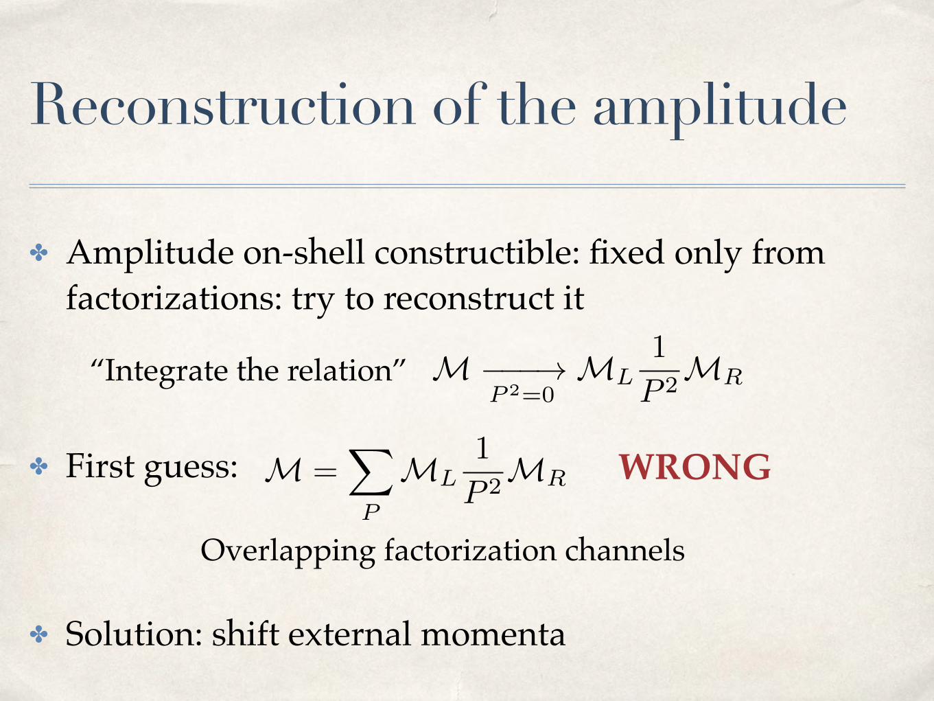
Reconstruction of the amplitude
✤ Amplitude on-shell constructible: fixed only from factorizations: try to reconstruct it
✤ First guess:
M ���!P 2=0
ML1
P 2MR“Integrate the relation”
M =X
P
ML1
P 2MR
Reconstruction of the amplitude
✤ Amplitude on-shell constructible: fixed only from factorizations: try to reconstruct it
✤ First guess:
✤ Solution: shift external momenta
M ���!P 2=0
ML1
P 2MR“Integrate the relation”
M =X
P
ML1
P 2MR WRONG
Overlapping factorization channels
Momentum shift
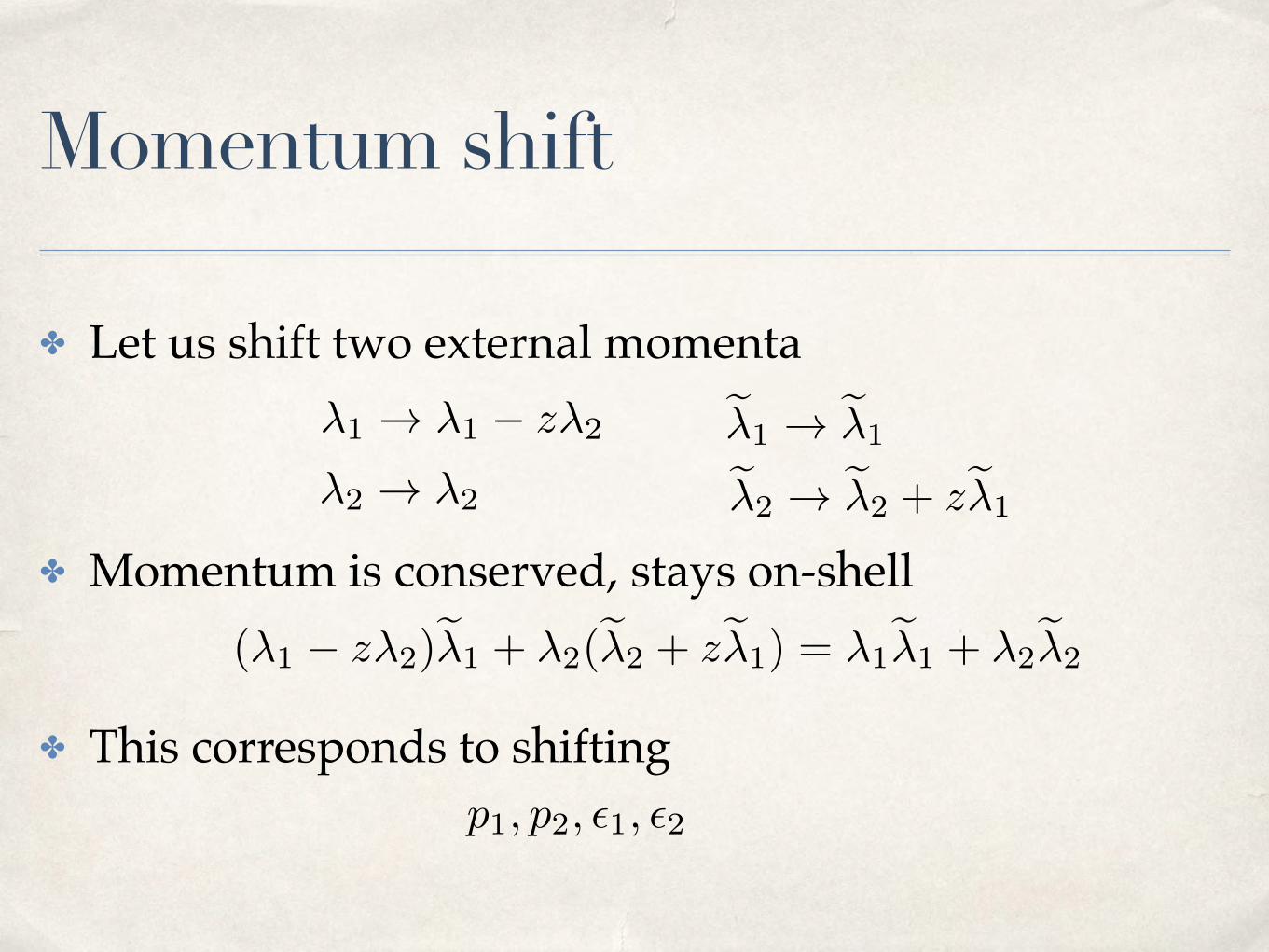
✤ Let us shift two external momenta
✤ Momentum is conserved, stays on-shell
✤ This corresponds to shifting
e�2 ! e�2 + ze�1
�1 ! �1 � z�2
(�1 � z�2)e�1 + �2(e�2 + ze�1) = �1e�1 + �2
e�2
e�1 ! e�1
�2 ! �2
p1, p2, ✏1, ✏2

Shifted amplitude
✤ On-shell tree-level amplitude with shifted kinematics
✤ Analytic structure
✤ Location of poles:
An(z) = A(p1(z), p2(z), p3, . . . , pn)
Pj(z) = Pj
Pj(z) = Pj � z�2e�1 p1 2 Pj
p2 2 Pj
if
if
otherwise
Pj(z) = Pj + z�2e�1
An(z) =N(z)Qj Pj(z)2
Shifted amplitude
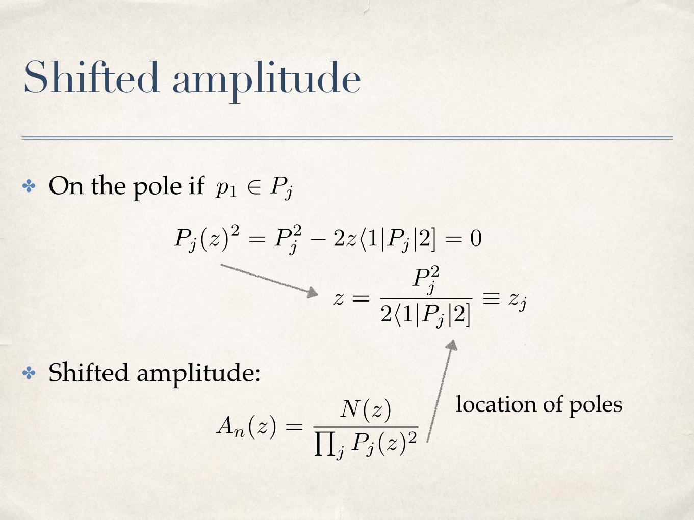
✤ On the pole if
✤ Shifted amplitude:
p1 2 Pj
Pj(z)2 = P 2
j � 2zh1|Pj |2] = 0
An(z) =N(z)Qj Pj(z)2
location of poles
z =P 2j
2h1|Pj |2]⌘ zj

Residue theorem
✤ Shifted amplitude
✤ Let us consider the contour integral
✤ Original amplitude
✤ Residue theorem:
Zdz
zAn(z) = 0
An = An(z = 0)
An(z) =N(z)Q
k(z � zk)
An +X
k
Res
✓An(z)
z
◆ �����z=zk
= 0
No pole at z ! 1
Residue at z = 0

Residue theorem
✤ Unitarity of shifted tree-level amplitude
An = �X
k
Res
✓An(z)
z
◆ �����z=zk
Residue on the pole
An(z) ������!Pj(z)2=0
AL(z)1
Pj(z)2AR(z)
Pj(z)2 = 0

Residue theorem
✤ Unitarity of shifted tree-level amplitude
An = �X
k
Res
✓An(z)
z
◆ �����z=zk
Residue on the pole Pj(z)2 = 2h1|Pj |2](zj � z) = 0
zj =P 2j
2h1|Pj |2]
An(z) ���!z=zj
AL(zj)1
2h1|Pj |2]AR(zj)

Residue theorem
An = �X
k
Res
✓An(z)
z
◆ �����z=zk
AL(zj)1
2h1|Pj |2]AR(zj)⇥
2h1|Pj |2]P 2j
= AL(zj)1
P 2j
AR(zj)
An = �X
j
AL(zj)1
P 2j
AR(zj)
Final formula
zj =P 2j
2h1|Pj |2]

BCFW recursion relations
An = �X
j
AL(zj)1
P 2j
AR(zj) zj =P 2j
2h1|Pj |2]
2 2
Chosen suchthat internal
line is on-shell
Sum over all distributions of legs keeping 1,2 on different sides
(Britto, Cachazo, Feng, Witten, 2005)
Comment on applicability
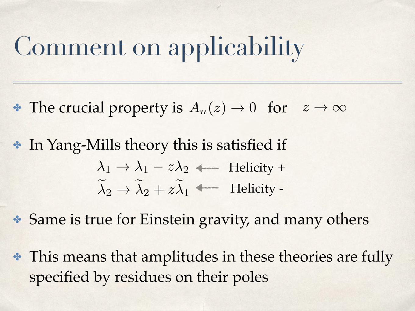
✤ The crucial property is for
✤ In Yang-Mills theory this is satisfied if
✤ Same is true for Einstein gravity, and many others
✤ This means that amplitudes in these theories are fully specified by residues on their poles
An(z) ! 0 z ! 1
�1 ! �1 � z�2
e�2 ! e�2 + ze�1
Helicity +Helicity -
Generalizations
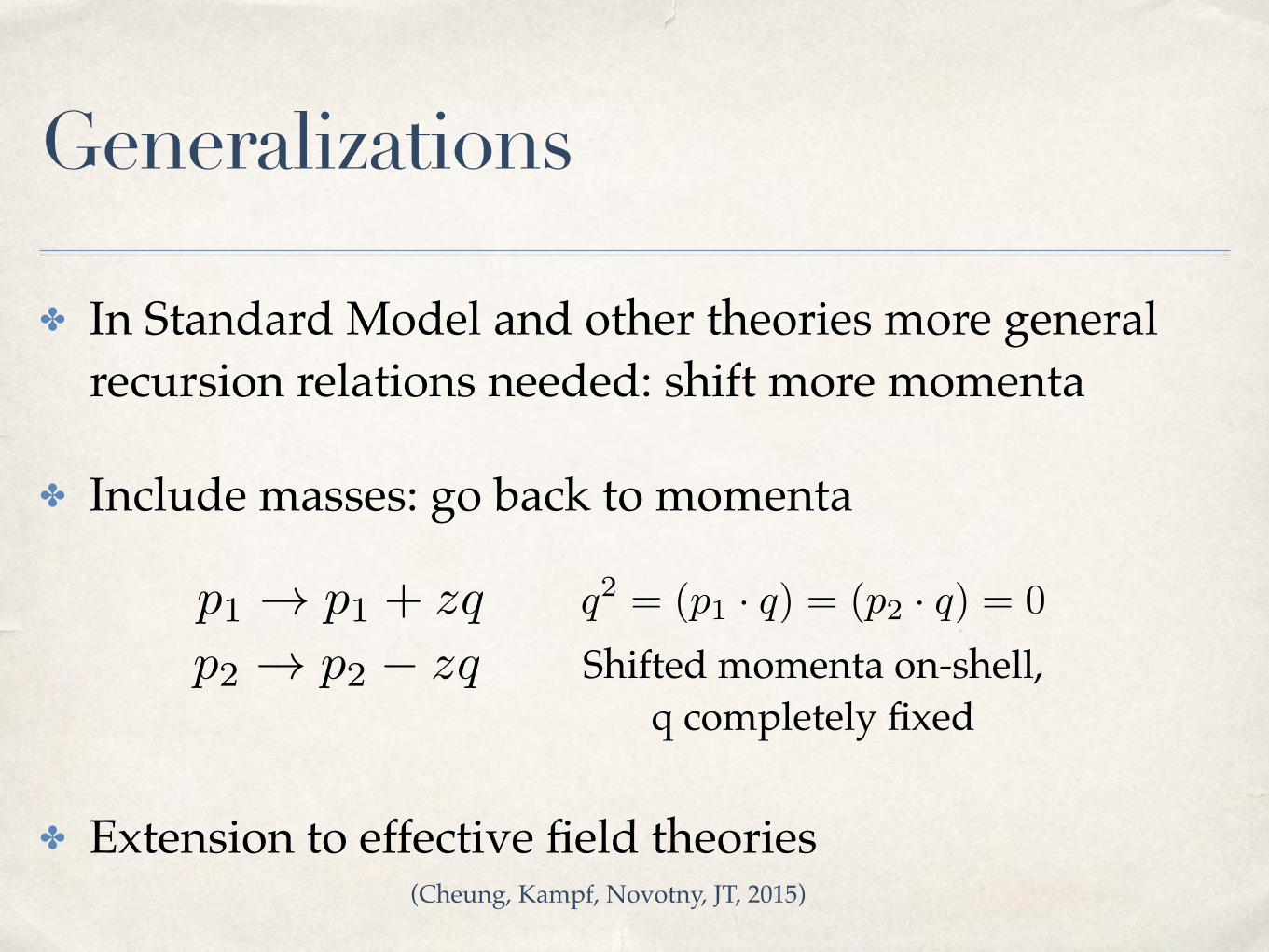
✤ In Standard Model and other theories more general recursion relations needed: shift more momenta
✤ Include masses: go back to momenta
✤ Extension to effective field theories
p1 ! p1 + zqp2 ! p2 � zq
q2 = (p1 · q) = (p2 · q) = 0
Shifted momenta on-shell,q completely fixed
(Cheung, Kampf, Novotny, JT, 2015)

Example: amplitudes of gluons
Color decomposition
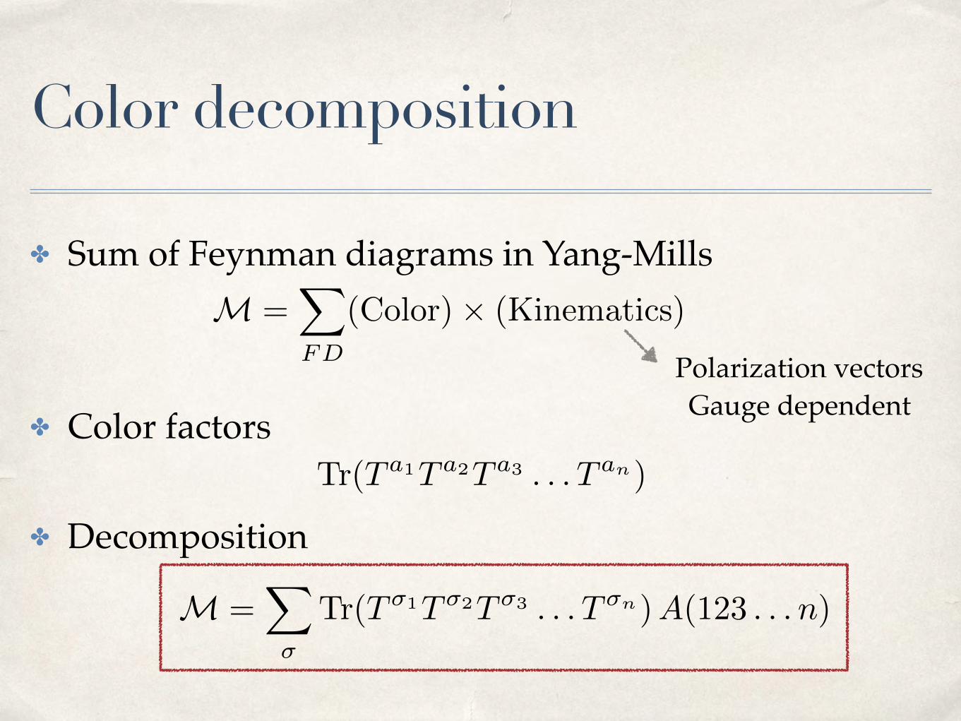
✤ Sum of Feynman diagrams in Yang-Mills
✤ Color factors
✤ Decomposition
Polarization vectorsGauge dependent
Tr(T a1T a2T a3 . . . T an)
M =X
�
Tr(T �1T �2T �3 . . . T �n)A(123 . . . n)
M =
X
FD
(Color)⇥ (Kinematics)
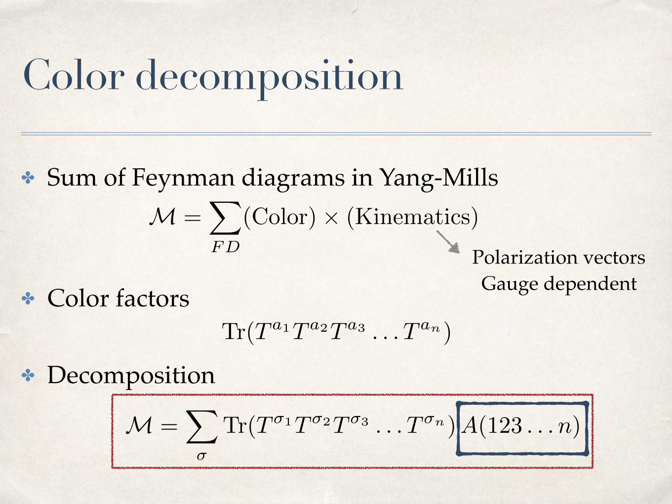
Color decomposition
✤ Sum of Feynman diagrams in Yang-Mills
✤ Color factors
✤ Decomposition
Polarization vectorsGauge dependent
Tr(T a1T a2T a3 . . . T an)
M =X
�
Tr(T �1T �2T �3 . . . T �n)A(123 . . . n)
M =
X
FD
(Color)⇥ (Kinematics)

Color ordered amplitude
Particles are ordered, other orderings: permutations
✤ This is a key object of our interest
✤ Consider:
A(123 . . . n)
All particles massless and on-shellAll momenta incomingHelicities fixed
Gauge invariant

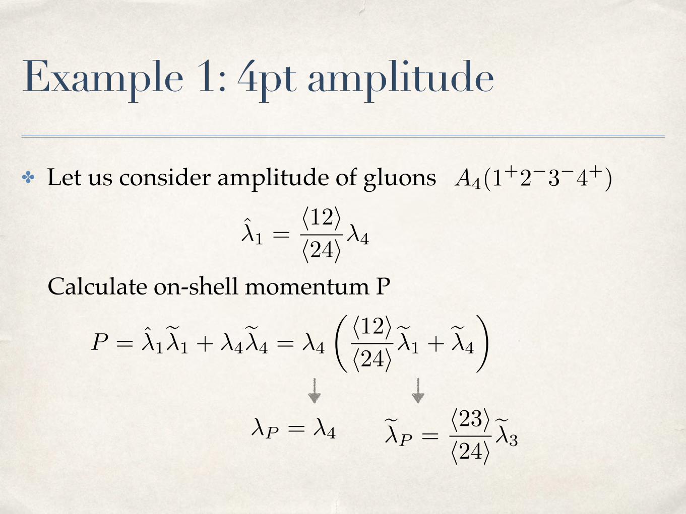
Example 1: 4pt amplitude
✤ Let us consider amplitude of gluons
P+P�Only one term
contributes
A4(1+2�3�4+)
1+ 2�
3�4+
�1 = �1 � z�2
e�2 = e�2 + ze�1
z takes the value whenP is on-shell momentum
[14]3
[1P ][4P ]
1
s23
h23i3
h2P ih3P i

Example 1: 4pt amplitude
✤ Let us consider amplitude of gluons A4(1+2�3�4+)
P 2 = h14i[14] = 0
h14i = h14i � zh24i = 0 z =h14ih24i
�1 = �1 � z�2 = �1 �h14ih24i�2 =
h12ih24i�4
We can now rewrite
e�2 = e�2 + ze�1 =[12]
[13]e�3
Shouten identity
Use of momentum conservation
Example 1: 4pt amplitude
✤ Let us consider amplitude of gluons A4(1+2�3�4+)
�1 =h12ih24i�4
P = �1e�1 + �4
e�4 = �4
✓h12ih24i
e�1 + e�4
◆Calculate on-shell momentum P
e�P =h23ih24i
e�3�P = �4

Example 1: 4pt amplitude
✤ Let us consider amplitude of gluons
P+P�
A4(1+2�3�4+)
1+ 2�
3�4+
[14]3
[1P ][4P ]
h23i3
h2P ih3P i
�1 =h12ih24i�4
e�2 =[12]
[13]e�3
�P = �4
e�P =h23ih24i
e�3
1
s23
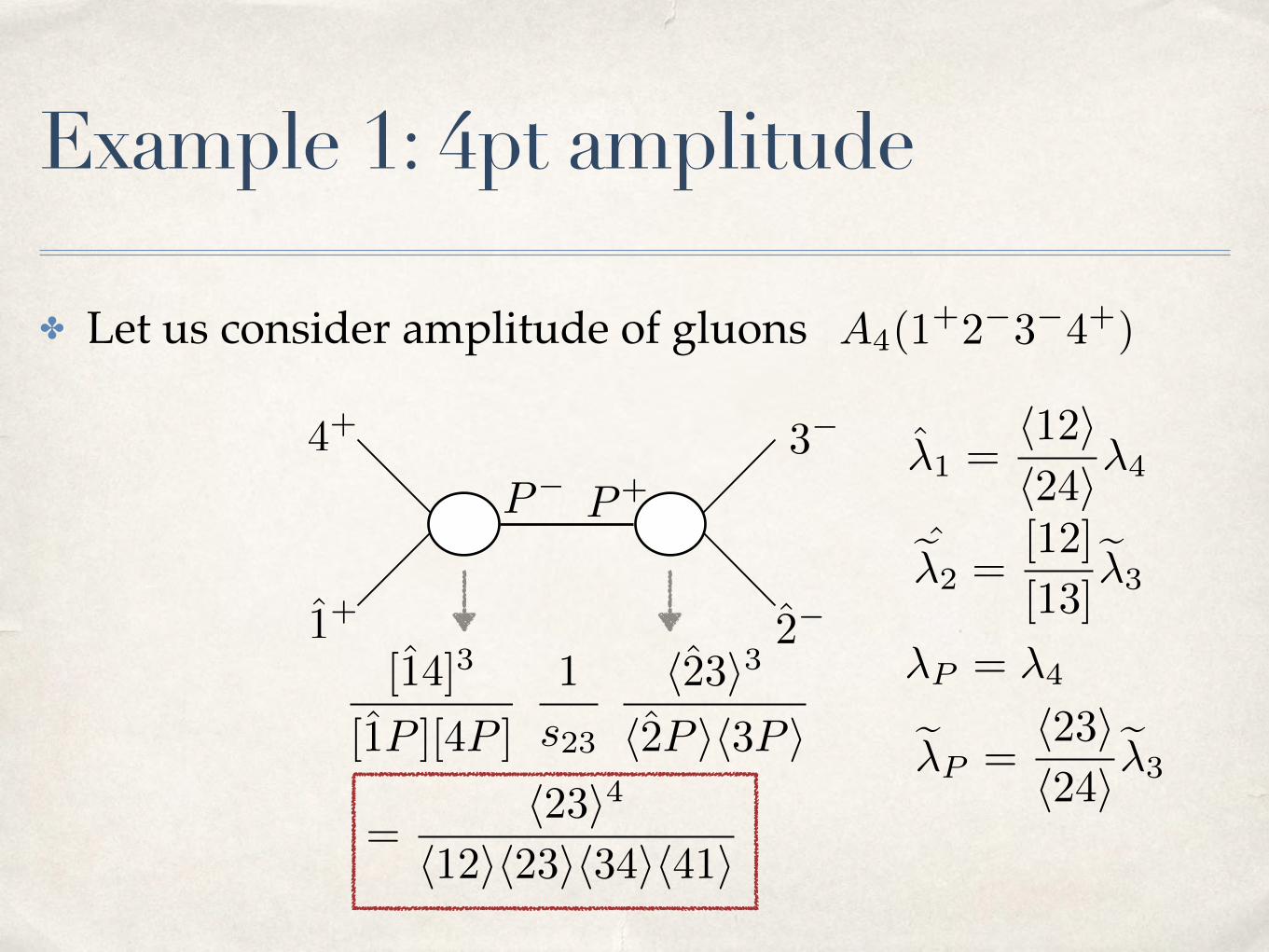
Example 1: 4pt amplitude
✤ Let us consider amplitude of gluons
P+P�
A4(1+2�3�4+)
1+ 2�
3�4+ �1 =h12ih24i�4
e�2 =[12]
[13]e�3
�P = �4
e�P =h23ih24i
e�3
=h23i4
h12ih23ih34ih41i
[14]3
[1P ][4P ]
1
s23
h23i3
h2P ih3P i

Example 1: 4pt amplitude
✤ Let us consider amplitude of gluons
P+P�
A4(1+2�3�4+)
1+ 2�
3�4+
One gauge invariantobject equivalent to
three Feynman diagrams

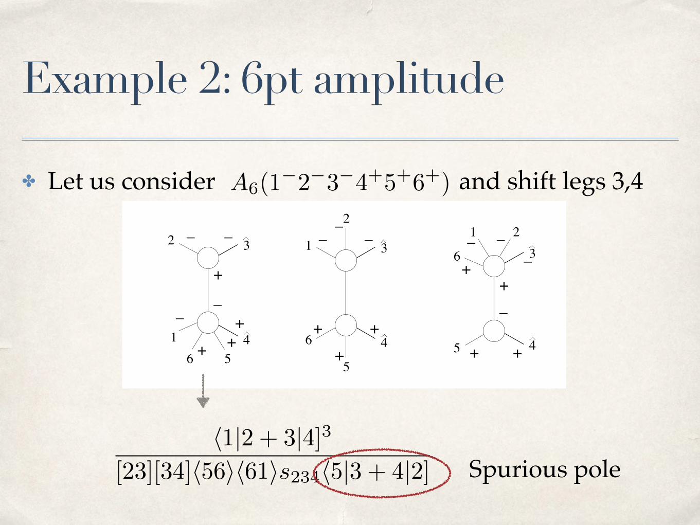
✤ Let us consider and shift legs 3,4
Example 2: 6pt amplitude
A6(1�2�3�4+5+6+)
4 4 4
3 3 3
(a) (b) (c)
156
1
21 2
6
55
6
2 __
_
__
_ _ __
+++
+ ++
++
__
++
+
Fig. 2: Configurations contributing to the six-gluon amplitude A6(1−, 2−, 3−, 4+, 5+, 6+).
Note that (a) and (c) are related by a flip and a conjugation. (b) vanishes for either
helicity configuration of the internal line.
This is shown in fig. 2. Note that for this helicity configuration, the middle graph
vanishes. Therefore, we are left with only two graphs to evaluate. Moreover, the two
graphs are related by a flip of indices composed with a conjugation. Therefore, only one
computation is needed.
Let us compute in detail the contribution coming from the first graph shown in
fig. 2(a). The contribution of this term is given by the product of two MHV amplitudes
times a propagator,
!⟨2 "3⟩3
⟨"3 "P ⟩⟨ "P 2⟩
#1
t[2]2
!⟨1 "P ⟩3
⟨ "P "4⟩⟨"4 5⟩⟨5 6⟩⟨6 1⟩
#
. (2.6)
This formula can be simplified by noting that
λ"3 = λ3,
λ"4 = λ4 −t[2]2
⟨3 2⟩[2 4]λ3,
⟨• "P ⟩ = −⟨•|2 + 3|4]
[ "P 4].
(2.7)
Using (2.7) it is straightforward to find (2.6)
⟨1|2 + 3|4]3
[2 3][3 4]⟨5 6⟩⟨6 1⟩t[3]2 ⟨5|3 + 4|2]. (2.8)
7
h1|2 + 3|4]3
[23][34]h56ih61is234h5|3 + 4|2]h1|2 + 3|4] = h12i[24] + h13i[34]
vs220 Feynman
diagrams
✤ Let us consider and shift legs 3,4
Example 2: 6pt amplitude
A6(1�2�3�4+5+6+)
4 4 4
3 3 3
(a) (b) (c)
156
1
21 2
6
55
6
2 __
_
__
_ _ __
+++
+ ++
++
__
++
+
Fig. 2: Configurations contributing to the six-gluon amplitude A6(1−, 2−, 3−, 4+, 5+, 6+).
Note that (a) and (c) are related by a flip and a conjugation. (b) vanishes for either
helicity configuration of the internal line.
This is shown in fig. 2. Note that for this helicity configuration, the middle graph
vanishes. Therefore, we are left with only two graphs to evaluate. Moreover, the two
graphs are related by a flip of indices composed with a conjugation. Therefore, only one
computation is needed.
Let us compute in detail the contribution coming from the first graph shown in
fig. 2(a). The contribution of this term is given by the product of two MHV amplitudes
times a propagator,
!⟨2 "3⟩3
⟨"3 "P ⟩⟨ "P 2⟩
#1
t[2]2
!⟨1 "P ⟩3
⟨ "P "4⟩⟨"4 5⟩⟨5 6⟩⟨6 1⟩
#
. (2.6)
This formula can be simplified by noting that
λ"3 = λ3,
λ"4 = λ4 −t[2]2
⟨3 2⟩[2 4]λ3,
⟨• "P ⟩ = −⟨•|2 + 3|4]
[ "P 4].
(2.7)
Using (2.7) it is straightforward to find (2.6)
⟨1|2 + 3|4]3
[2 3][3 4]⟨5 6⟩⟨6 1⟩t[3]2 ⟨5|3 + 4|2]. (2.8)
7
h1|2 + 3|4]3
[23][34]h56ih61is234h5|3 + 4|2] Spurious pole

Remark on BCFW
✤ Extremely efficient (3 vs 220 for 6pt, 20 vs 34300 for 8pt)
✤ Terms in BCFW recursion relations
✤ Amplitude = sum of these terms dictated by unitarity
✤ Note: not all factorization channels are present
Gauge invariantSpurious poles
when 1,2 are on the same side

Unitarity methods

One-loop amplitudes
✤ Sum of Feynman diagrams
✤ Re-express as basis of canonical integrals
M1�loop =X
j
ZdI
j
dIj = d4` Ijwhere
M1�loop =X
j
aj
ZdI(4)
j
+X
j
bj
ZdI(3)
j
+X
j
cj
ZdI(2)
j
+R
Box Triangle Bubble
Rational
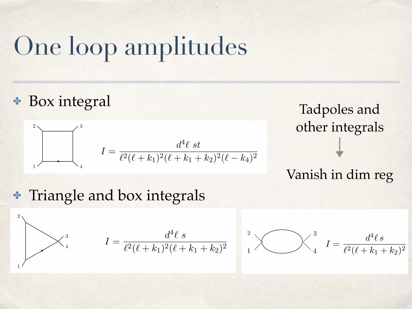
✤ Box integral
✤ Triangle and box integrals
I =d4` s
`2(`+ k1 + k2)2
One loop amplitudesSingularities of loop integrals
I Example: box integral
1
2 3
4
I =d4` st
`2(`+ k1
)2(`+ k1
+ k2
)2(`� k4
)2
I Examples of integrals with non-logarithmic singularities:
I =d4`
(`2)2(`+ k1
)2(`+ k1
+ k2
)2, I =
d4`
`2(`+ k1
)2(`+ k2
)2(`+ k3
)2
I At higher loops: multiple poles! Special numerator needed to cancel them.
Poles at infinity
• Example: triangle integral
1
2
3
4I =
d4` s
`2(`+ k1
)2(`+ k1
+ k2
)2
I Triple cut: `2 = (`+ k1
)2 = (`+ k1
+ k2
)2 = 0
I Solution: `� k1
= ↵�1
f�2
I Residue on this cut: I =d↵
↵
I Pole for ↵ ! 1 which implies ` ! 1.
Tadpoles and other integrals
Vanish in dim reg
1
2 3
4
UV divergent
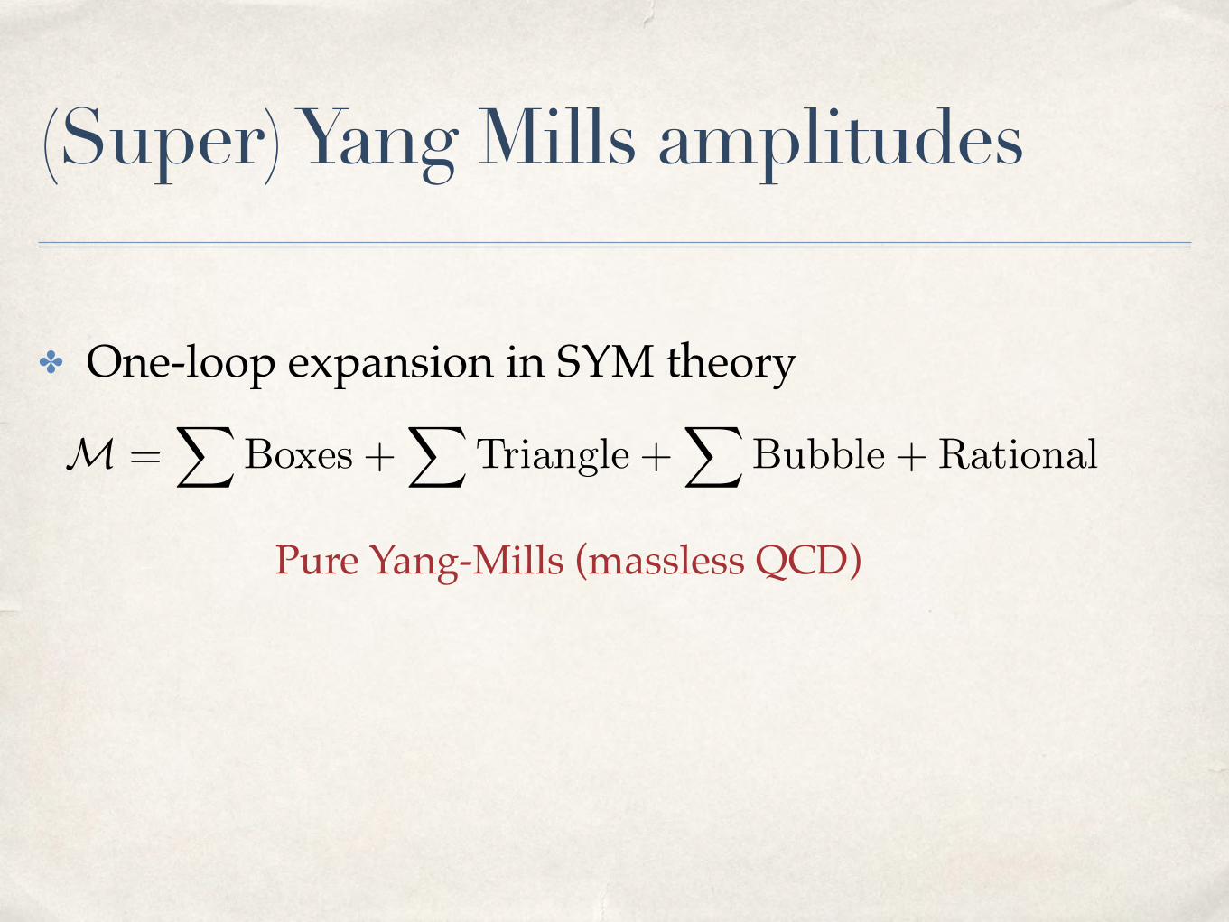
(Super) Yang Mills amplitudes
✤ One-loop expansion in SYM theory
M =
XBoxes +
XTriangle +
XBubble + Rational
Pure Yang-Mills (massless QCD)
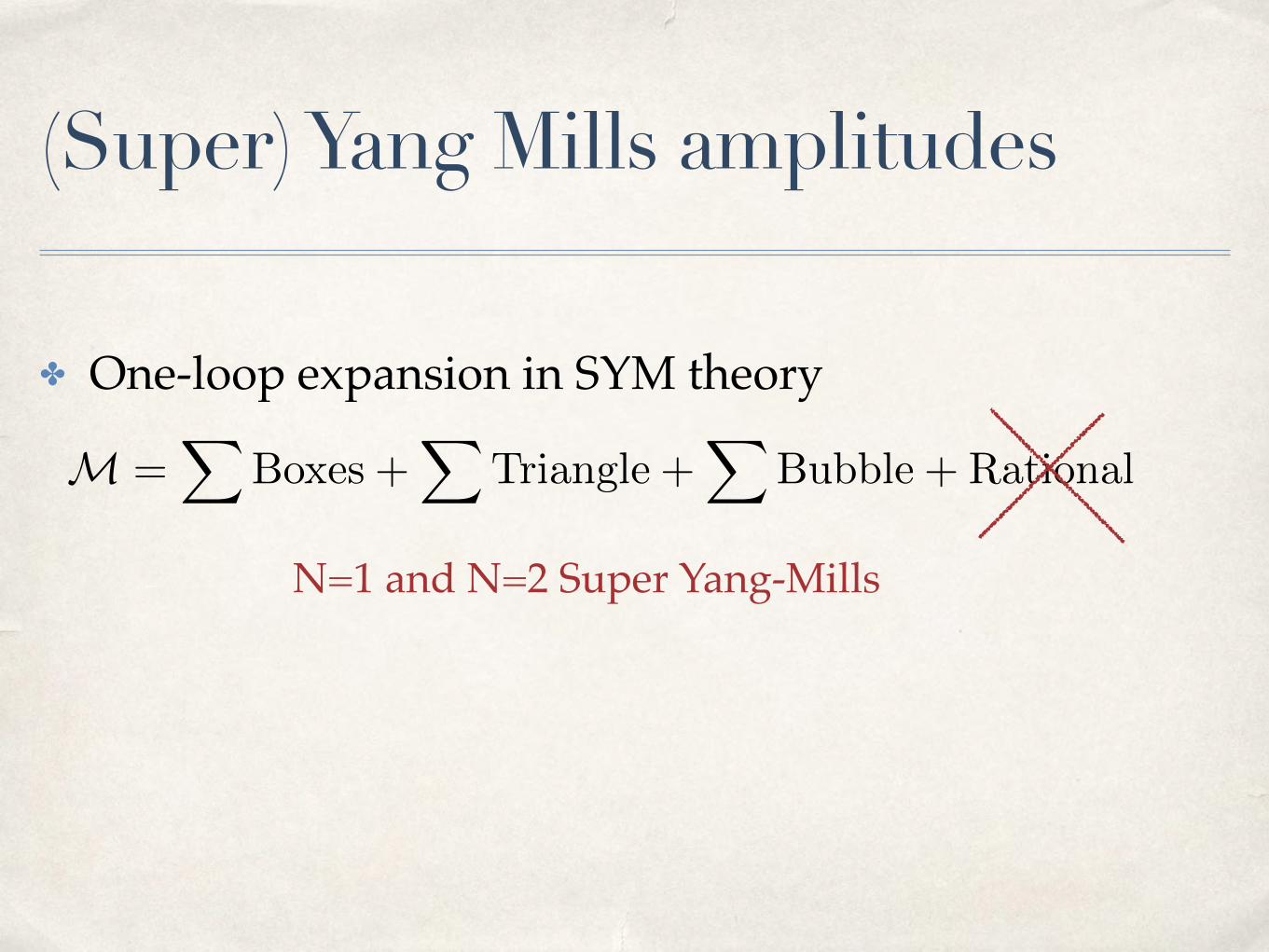
(Super) Yang Mills amplitudes
✤ One-loop expansion in SYM theory
M =
XBoxes +
XTriangle +
XBubble + Rational
N=1 and N=2 Super Yang-Mills

(Super) Yang Mills amplitudes
✤ One-loop expansion in SYM theory
✤ Note that it is UV finite at 1-loop, but also all loops
M =
XBoxes +
XTriangle +
XBubble + Rational
N=4 Super Yang-Mills
One loop expansion
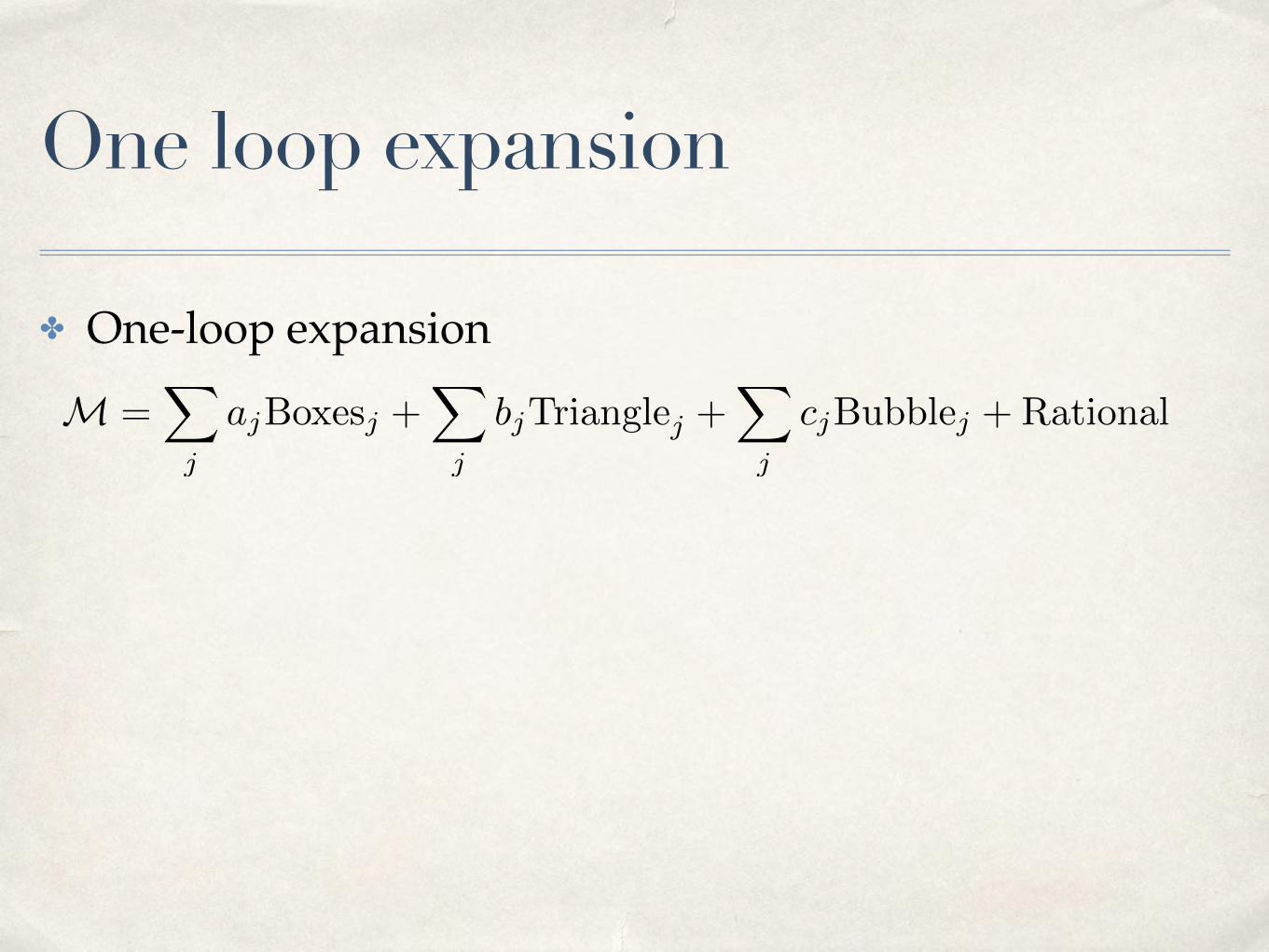
✤ One-loop expansion
M =
X
j
ajBoxesj +X
j
bjTrianglej +X
j
cjBubblej +Rational

One loop expansion
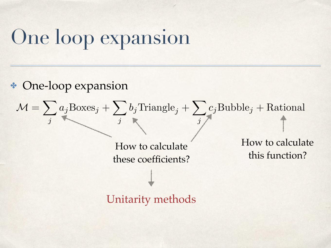
✤ One-loop expansion
M =
X
j
ajBoxesj +X
j
bjTrianglej +X
j
cjBubblej +Rational
How to calculatethese coefficients?
How to calculatethis function?
One loop expansion
✤ One-loop expansion
M =
X
j
ajBoxesj +X
j
bjTrianglej +X
j
cjBubblej +Rational
How to calculatethese coefficients?
How to calculatethis function?
Unitarity methods
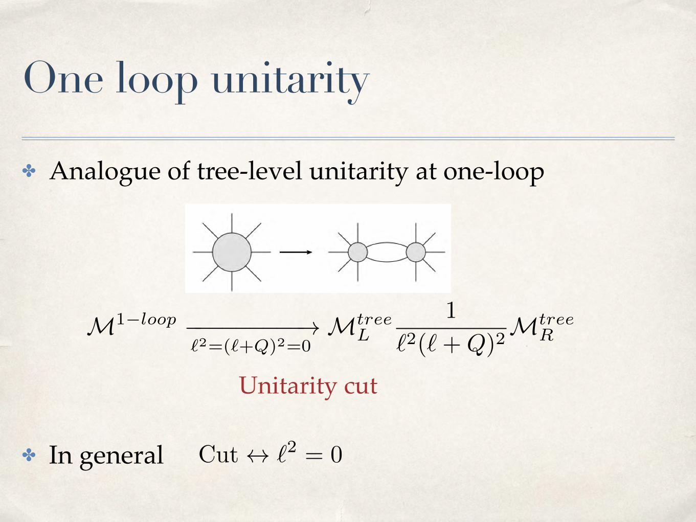
One loop unitarity
✤ Analogue of tree-level unitarity at one-loop
✤ In general
M1�loop ���������!`
2=(`+Q)2=0Mtree
L
1
`2(`+Q)2Mtree
R
Unitarity cut
Cut $ `2 = 0

One-loop unitarity
✤ Higher cuts
`2 = (`+Q1)2 = (`+Q2)
2 = 0
Triple cut Quadruple cut`2 = (`+Q1)
2 = (`+Q2)2 = (`+Q3)
2 = 0
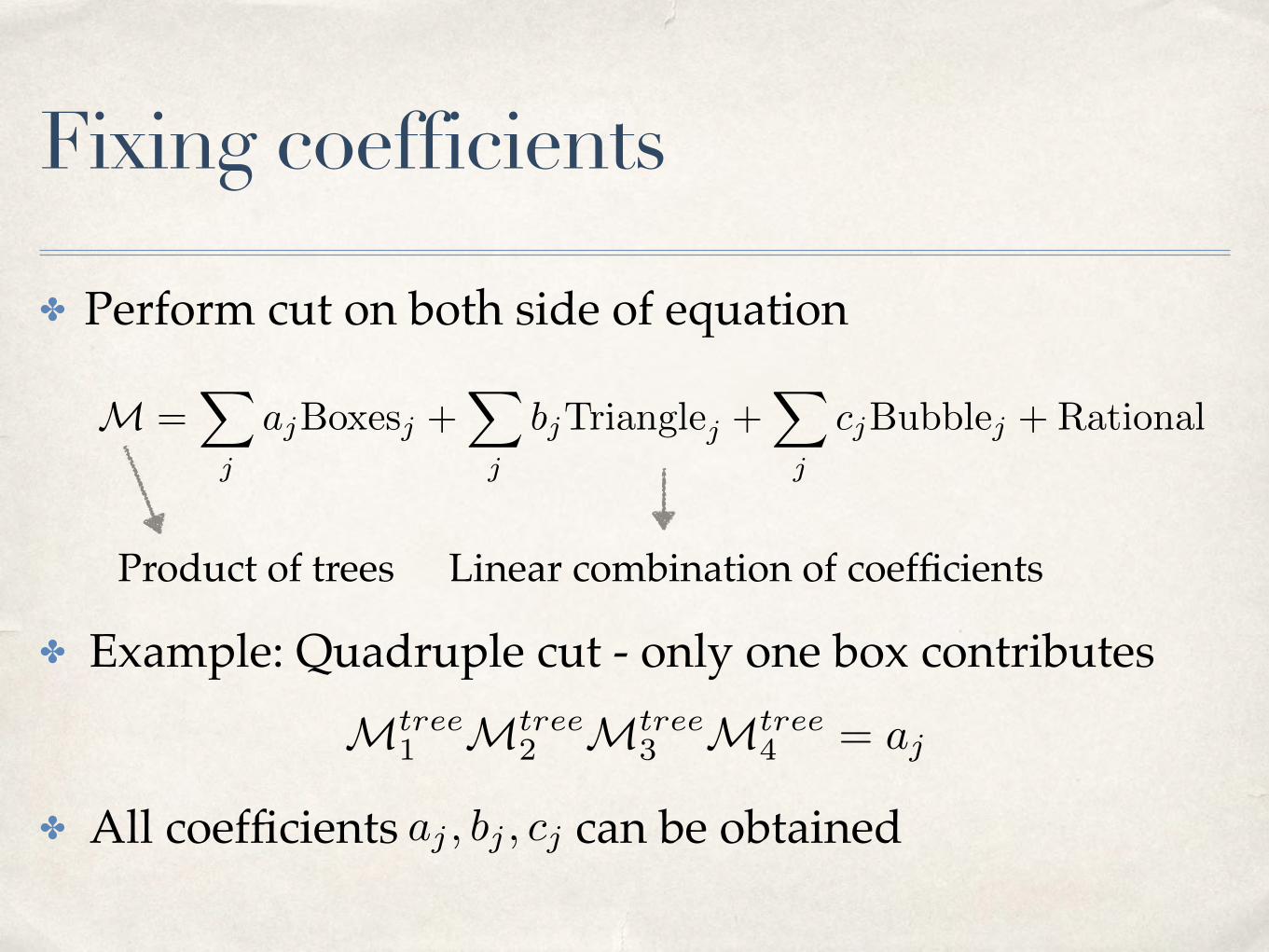
Fixing coefficients
✤ Perform cut on both side of equation
✤ Example: Quadruple cut - only one box contributes
✤ All coefficients can be obtained
M =
X
j
ajBoxesj +X
j
bjTrianglej +X
j
cjBubblej +Rational
Product of trees
Mtree1 Mtree
2 Mtree3 Mtree
4 = aj
aj , bj , cj
Linear combination of coefficients
Unitarity methods
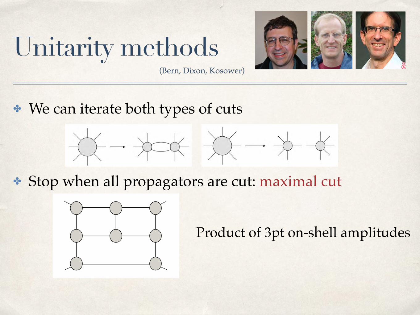
✤ We can iterate both types of cuts
✤ Stop when all propagators are cut: maximal cut
Product of 3pt on-shell amplitudes
(Bern, Dixon, Kosower)
Unitarity methods
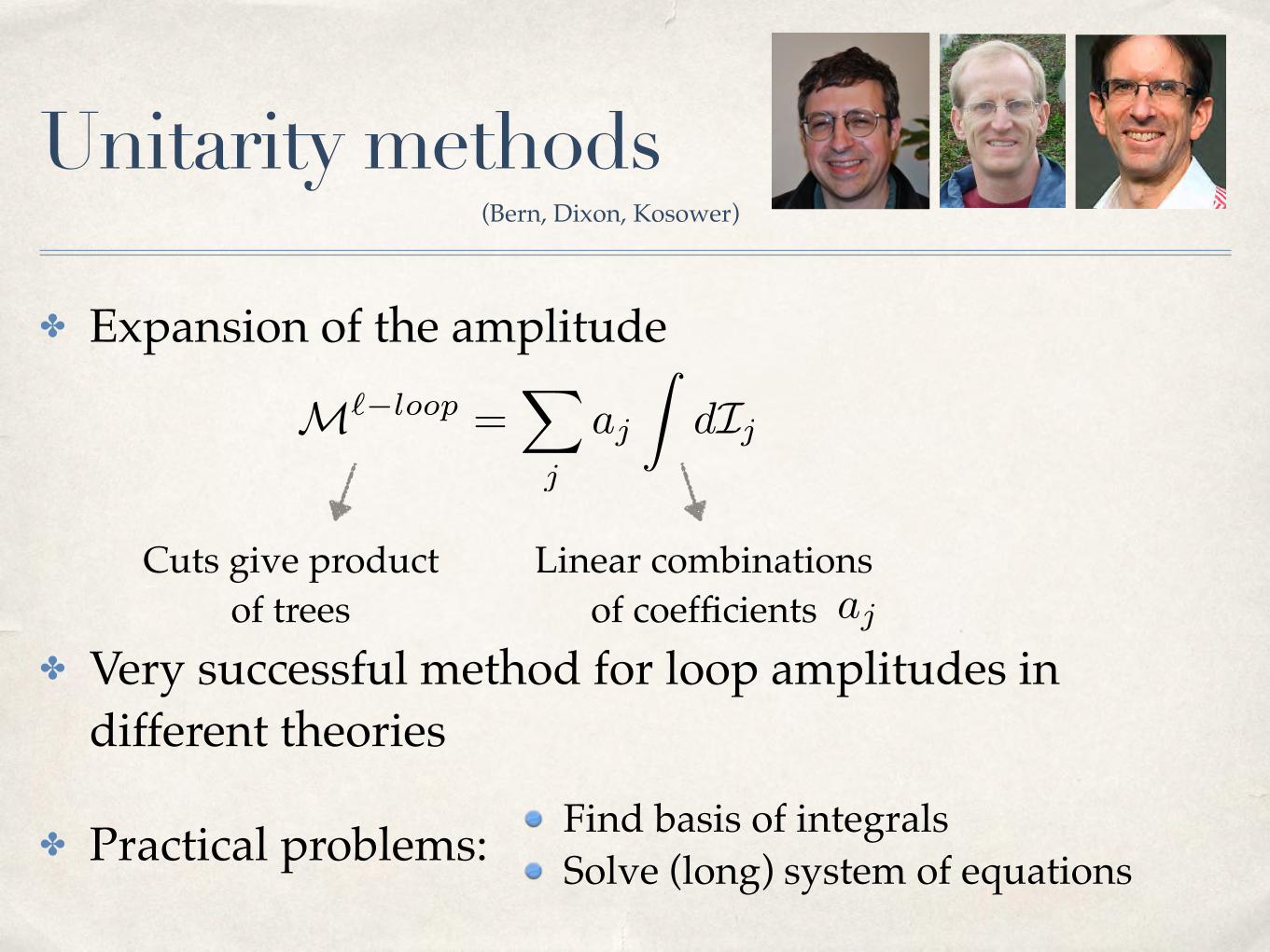
✤ Expansion of the amplitude
✤ Very successful method for loop amplitudes in different theories
✤ Practical problems:
M`�loop =X
j
aj
ZdI
j
Cuts give productof trees
Linear combinationsof coefficients aj
Find basis of integralsSolve (long) system of equations
(Bern, Dixon, Kosower)

Unitarity methods
✤ Results in susy theories and QCD
1 (i) 4
32
5
6
(h)
2
41
3
5
7 6
1 4(g)
2 3
5
(f)1
2 3
4
5
(e) 41
2 3
5
3
(d)
2
41
(a)
32
1 4 4(b)
32
1
2
4(c)1
3
Basis of integrals for 3-loop amplitudes in N=4 SYM and N=8 SUGRA Black Hat
(Bern, Dixon, Kosower)

On-shell good, off-shell bad
✤ Feynman diagrams: off-shell objects
✤ Unitarity methods:
✤ Recursion relations
✤ Next direction: loosing manifest locality and unitarity
Off-shell objects
On-shell objects
Cut[M] = Cut[Basis of integrals]
M ⇠ ML MR
LocalityUnitarity
On-shell objects
Locality lostUnitarity
On-shell diagrams(Arkani-Hamed, Bourjaily, Cachazo, Goncharov, Postnikov, JT 2012)

Atoms of amplitudes
What are natural gauge invariant objects?

Atoms of amplitudes
What are natural gauge invariant objects?
Scattering amplitudes
✤ Recursion relations, unitarity methods: products of amplitudes
✤ Iterative procedure: reduces to elementary amplitudes
✤ In most interesting theories these are three point

✤ Two options
Three point kinematics
pµ = �µaa�a
e�a
Spinor helicity variables
h12i = ✏ab�1a�2b
[12] = ✏ab�1a�2b
�1 ⇠ �2 ⇠ �3
e�1 ⇠ e�2 ⇠ e�3Two solutions for
3pt kinematicsp21 = p22 = p23 = (p1 + p2 + p3) = 0
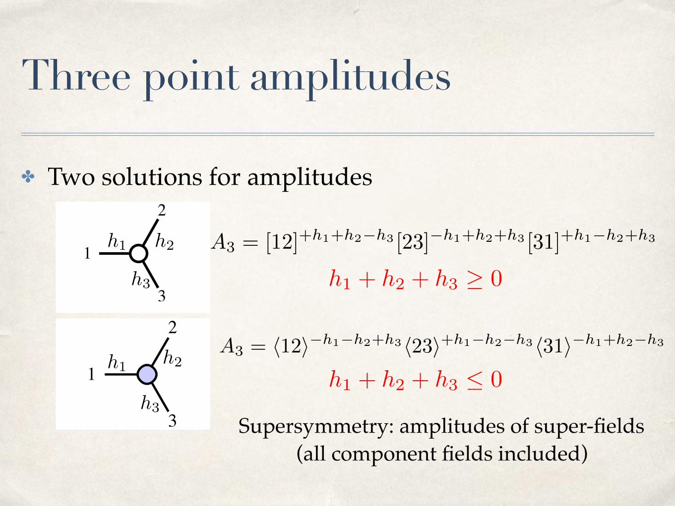
✤ Two solutions for amplitudes
Three point amplitudes
h1 h2
h3
h1h2
h3
h1 + h2 + h3 0
h1 + h2 + h3 � 0
A3 = h12i�h1�h2+h3h23i+h1�h2�h3h31i�h1+h2�h3
A3 = [12]+h1+h2�h3 [23]�h1+h2+h3 [31]+h1�h2+h3
Supersymmetry: amplitudes of super-fields(all component fields included)

✤ In N=4 SYM: no need to specify helicities
Three point amplitudes
A(1)3 =
�4(p1 + p2 + p3)�4([23]e⌘1 + [31]e⌘2 + [12]e⌘3)[12][23][31]
A(2)3 =
�4(p1 + p2 + p3)�8(�1e⌘1 + �2e⌘2 + �3e⌘3)h12ih23ih31i
Fully fixed in any QFT up to coupling
Easy book-keeping
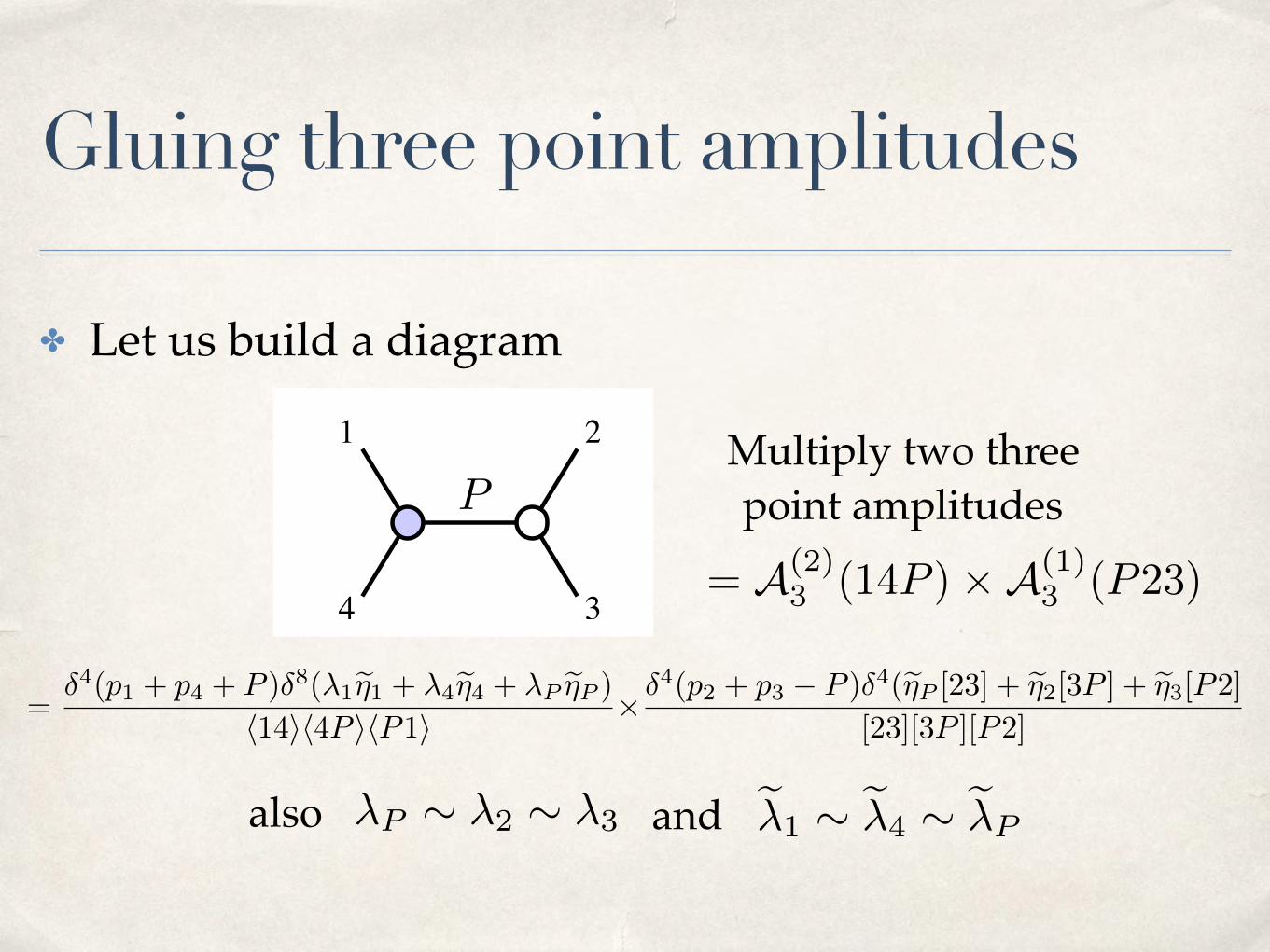
✤ Let us build a diagram
P
Gluing three point amplitudes
= A(2)3 (14P )⇥A(1)
3 (P23)
Multiply two threepoint amplitudes
=�4(p1 + p4 + P )�8(�1e⌘1 + �4e⌘4 + �P e⌘P )
h14ih4P ihP1i ⇥�4(p2 + p3 � P )�4(e⌘P [23] + e⌘2[3P ] + e⌘3[P2]
[23][3P ][P2]
also �P ⇠ �2 ⇠ �3 e�1 ⇠ e�4 ⇠ e�Pand
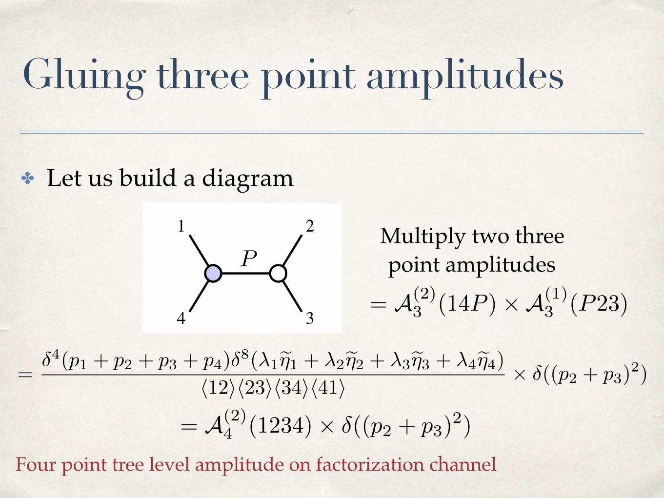
✤ Let us build a diagram
P
Gluing three point amplitudes
= A(2)3 (14P )⇥A(1)
3 (P23)
Multiply two threepoint amplitudes
=�4(p1 + p2 + p3 + p4)�8(�1e⌘1 + �2e⌘2 + �3e⌘3 + �4e⌘4)
h12ih23ih34ih41i ⇥ �((p2 + p3)2)
= A(2)4 (1234)⇥ �((p2 + p3)
2)
Four point tree level amplitude on factorization channel

P
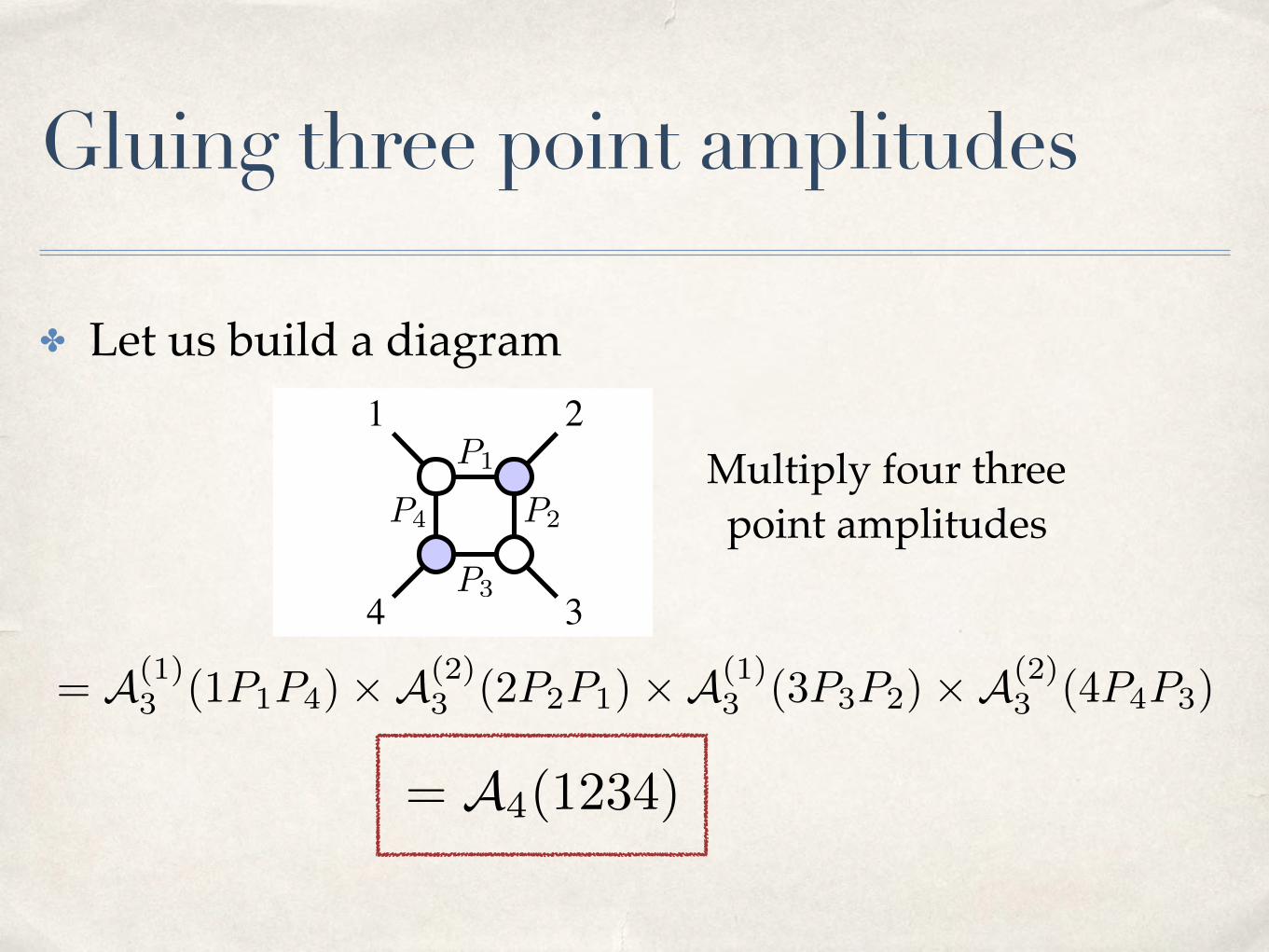
✤ Let us build a diagram
Gluing three point amplitudes
Multiply four threepoint amplitudes
P1
P2
P3
P4
= A(1)3 (1P1P4)⇥A(2)
3 (2P2P1)⇥A(1)3 (3P3P2)⇥A(2)
3 (4P4P3)
P
✤ Let us build a diagram
Gluing three point amplitudes
Multiply four threepoint amplitudes
P1
P2
P3
P4
= A(1)3 (1P1P4)⇥A(2)
3 (2P2P1)⇥A(1)3 (3P3P2)⇥A(2)
3 (4P4P3)
= A4(1234)
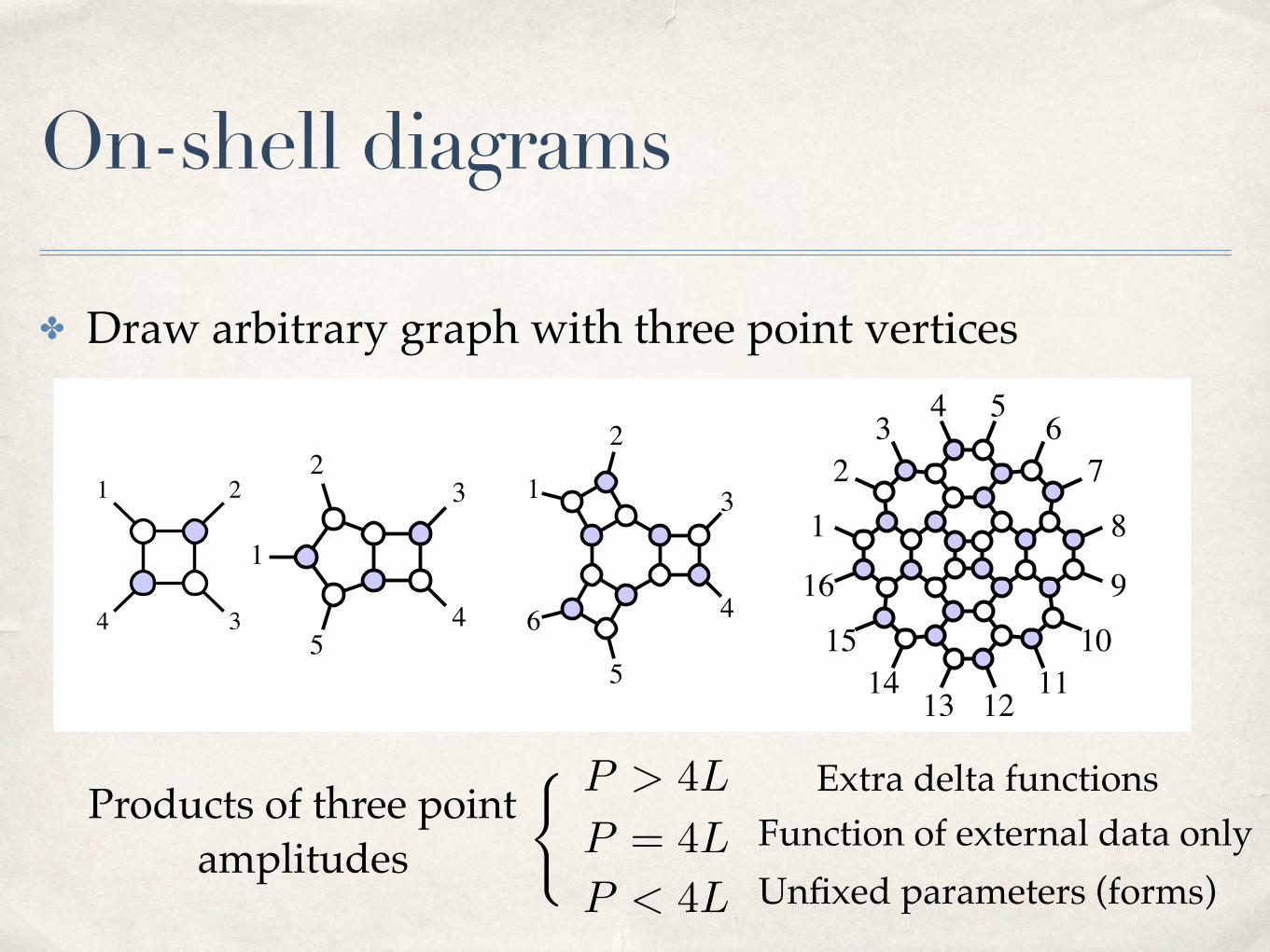
✤ Draw arbitrary graph with three point vertices
On-shell diagrams
Products of three point amplitudes
P > 4L
P = 4L
P < 4L
( Extra delta functionsFunction of external data onlyUnfixed parameters (forms)
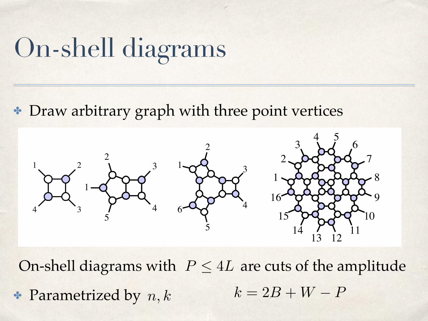
✤ Draw arbitrary graph with three point vertices
✤ Parametrized by
On-shell diagrams with are cuts of the amplitude
On-shell diagrams
P 4L
n, k k = 2B +W � P

✤ Draw arbitrary graph with three point vertices
On-shell diagrams
Question: Can we build amplitude from on-shell diagrams?

Recursion relations
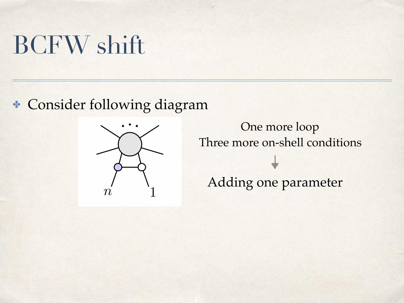
✤ Consider following diagram
BCFW shift
n 1
One more loopThree more on-shell conditions
Adding one parameter

BCFW shift
✤ Consider following diagram
n 1
One more loopThree more on-shell conditions
Adding one parameterz�1
e�n
New formula: K1(z) =dz
zK0(z)

BCFW shift
✤ Consider following diagram
n 1
One more loopThree more on-shell conditions
Adding one parameterz�1
e�n
New formula: K1(z) =dz
zK0(z)
Old on-shell diagramwith shift
�n ! �n + z�1
e�1 ! e�n � ze�1

BCFW recursion relations
✤ Suppose the blob is the amplitude
✤ Cauchy formula
n 1
= An(z)
Shifted amplitude �n ! �n + z�1
e�1 ! e�n � ze�1
@An(z) = 0
Take the residue on z = zk $ Erase an edge in the diagram
An

✤ Recursion relations for amplitude
✤ Tree-level amplitude = sum of on-shell diagrams
✤ Term-by-term identical to terms in BCFW recursion
=
BCFW recursion relations
+X
L,R0

✤ Four point: only one factorization channel
✤ Five point amplitude
Simple examples
BCFW bridgeon 3,4
Bridge 5,1 on 3pt and 4pt amplitudes

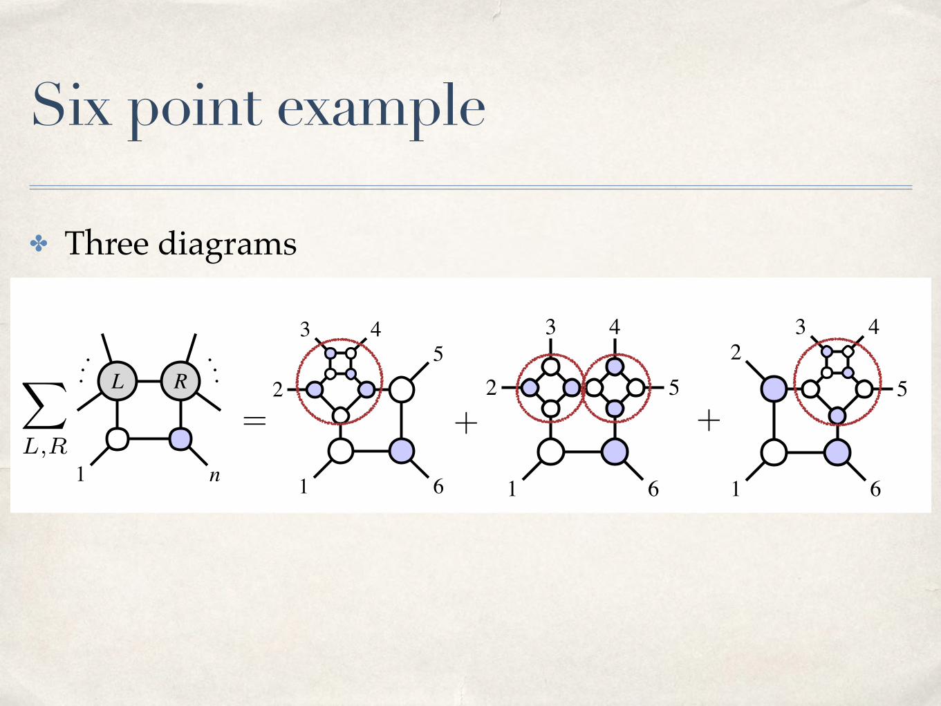
✤ Three diagrams
+
Six point example
+=
X
L,R
✤ Three diagrams
+
Six point example
+=
X
L,R
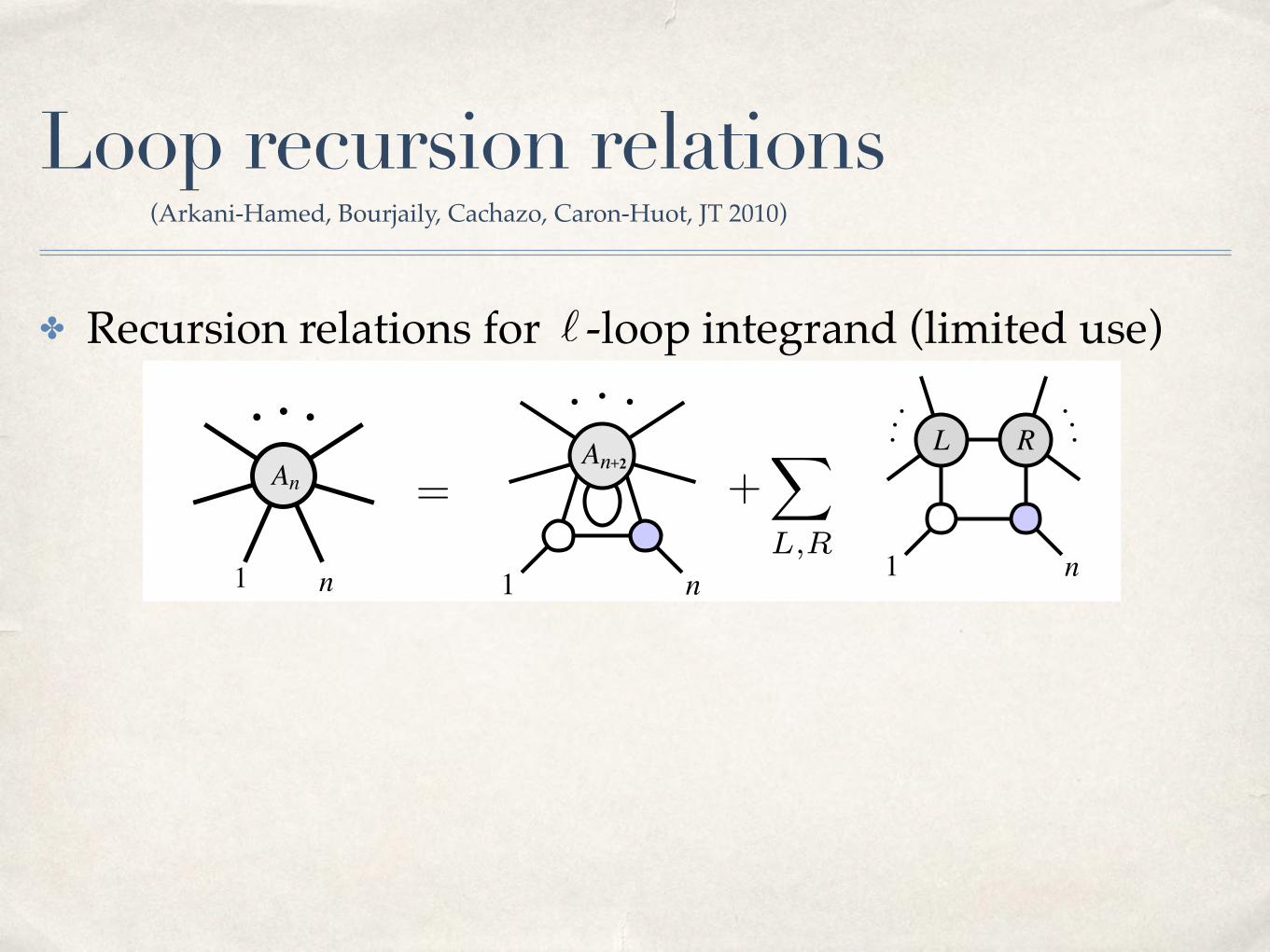
Loop recursion relations
✤ Recursion relations for -loop integrand (limited use)
+X
L,R
=
`
(Arkani-Hamed, Bourjaily, Cachazo, Caron-Huot, JT 2010)

Loop recursion relations
✤ Recursion relations for -loop integrand (limited use)
✤ Loop orders:
✤ New loop momentum
+X
L,R
=
(`� 1) `1, `2`1 + `2 = `
`
`(L) = `(L)0 + z�1
e�n
(`(L)0 )2 = 0
(Arkani-Hamed, Bourjaily, Cachazo, Caron-Huot, JT 2010)
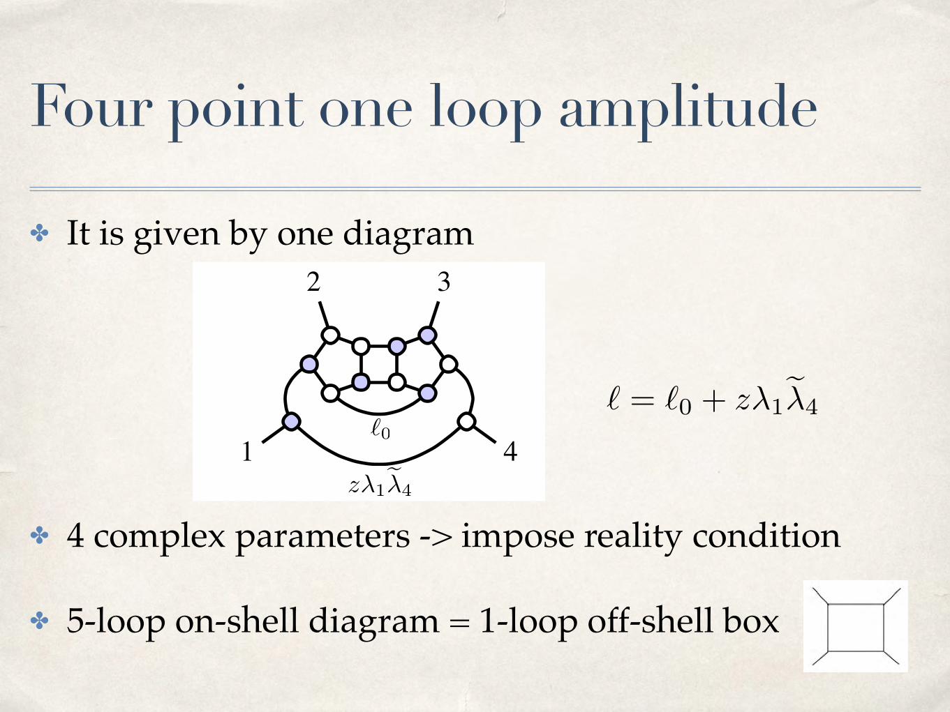
✤ It is given by one diagram
✤ 4 complex parameters -> impose reality condition
✤ 5-loop on-shell diagram = 1-loop off-shell box
`0
Four point one loop amplitude
z�1e�4
` = `0 + z�1e�4

✤ Tree-level recursion: diagrams with contribute
✤ These are also leading singularities of loop amplitudes
✤ Loop level: free parameters left
Dimensionality of diagrams
rational functions of external kinematicsno delta functions, no free parameters
P = 4L
components of loop momentaP = 16free = 4L� PL = 5free = 4
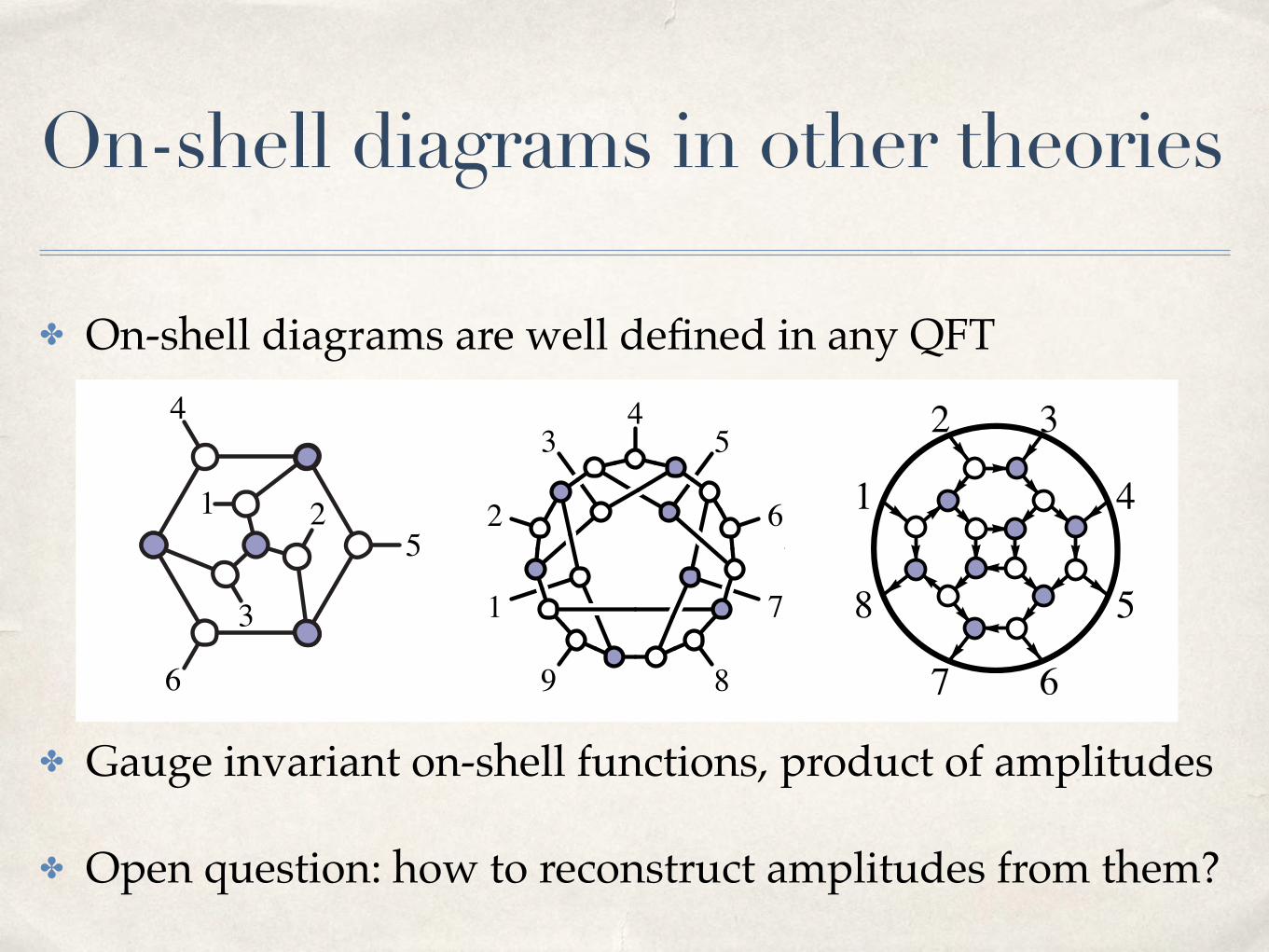
✤ On-shell diagrams are well defined in any QFT
✤ Gauge invariant on-shell functions, product of amplitudes
✤ Open question: how to reconstruct amplitudes from them?
On-shell diagrams in other theories
Let us now show that n= nW 0 , which implies that there are no black-to-black
internal edges. Let us say the number of white multi-vertices is n+q; we want to
show that q=0. From the definition of k,
k = 2nB + nW 0 � nI = 2nB + (n+ q)� nI = 3nB + 2 + q � nI , (2.5)
from which we see that for k = 2, 3nB = nI q. But 3nB � nI on general grounds,
and so we must have that q=0, and hence 3nB=nI . Because q=0, there is one leg
connected to each white multi-vertex (nW 0 =n); and because 3nB=nI , there can be
no black-to-black internal edges. Thus every black vertex connects to precisely three
external legs via white multi-vertices, as we wanted to prove.
Therefore, any MHV (k = 2) on-shell diagram corresponding to an ordinary
function of the external data (n�=0) with kinematical support will involve precisely
(n 2) black vertices, each of which is attached to exactly three external legs via
white vertices. Thus, we can label any such diagram by a set T consisting of triplets
⌧ 2T of leg labels for each of the (n 2) black vertices.
We can illustrate how this labeling works with the following examples:
⇢(1 2 4)
(2 3 4)
� 8<
:
(1 2 3)
(1 3 4)
(1 3 5)
9=
; (2.6)
8>>><
>>>:
(1 2 3)
(2 5 6)
(3 4 6)
(4 5 1)
9>>>=
>>>;
8>>>>>>>>><
>>>>>>>>>:
(1 2 4)
(1 8 9)
(2 9 3)
(3 6 4)
(4 6 5)
(6 8 7)
(6 9 8)
9>>>>>>>>>=
>>>>>>>>>;
(2.7)
Notice that because there is no preferred way to order the external legs of a non-
planar diagram, there is no preferred way to order the triples. And so while we
have chosen a particular ordering for each triple in the examples above, these choices
should be viewed as completely arbitrary.
– 5 –
14. On-Shell Diagrams with N < 4 Supersymmetries
On-shell diagrams can be defined for any theory with fundamental trivalent vertices,
and in particular for gauge theories with any number, N , of supersymmetries. There
is obviously a rich structure to be unearthed here; in this short section we will
content ourselves with setting-up some of the basic formalism and highlighting the
central new mathematical object that makes an appearance—reflecting the physics
of ultraviolet singularities which are present in theories with less supersymmetry.
Let us begin our discussion by focusing on non-supersymmetric theories, those
of “N = 0”. It is useful to represent the helicities involved in each basic 3-particle
vertex by giving each of the edges an orientation:
and (14.1)
We can then glue these vertices together to build-up more complex on-shell diagrams
as before—leading to, for example:
(14.2)
In such decorated on-shell diagrams, the arrows are useful because they automatically
encode the helicities of the internal particles involved. In general, we consider the
particles as Grassmann coherent states labeled by e⌘I for I = 1, . . . ,N . In theories
with N < 4 supersymmetry, we have “+” and “�” multiplets, which include gluons
of helicity ±1 as their top components, respectively; thus, on-shell diagrams must be
labeled in exactly the same way for any N < 4.
The Grassmannian formalism is just as powerful in integrating over the phase
space of the internal particles regardless of the amount of supersymmetry. However,
when N < 4, the diagrams really are fundamentally oriented, whereas for N = 4
such an orientation merely encodes a convenient translation of the on-shell diagram
into a particular gauge-fixed matrix-representative C 2 G(k, n). If the k incoming
“source” indices are from a set A and the (n k) outgoing “sink” indices are from a,
we find exactly the same linear relation between the external kinematical data:YA
�2�e�
A
� cAa
e�a
�YA
�N�e⌘
A
� cAa
e⌘a
�Ya
�2��a
+ cAa
�A
�, (14.3)
– 101 –

Thank you for attention!