scan converting lines line equation algorithmpang/160/f12/slides/dda.pdfscan converting lines •...

52438S Computer Graphics Winter 2004 Kari Pulli1

Scan converting lines• Input:

• two pixel locations (x1,y1) and (x2,y2) in device coordinates

• Goal:• determine the intermediate pixels to paint to connect the

points


Line equation algorithm• Line equation: y = mx + b

• What’s the problem?

def line_eq(x1,y1,x2,y2):m = (y2-y1) / float(x2-x1)b = y1 - m * x1if x2 > x1: dx = 1else: dx = -1while x1 != x2:

y = m * x1 + bpaint(x1, round(y))x1 += dx

If the slope is > 1, the line is not continuous,pixels are skipped


DDA algorithm• DDA = Digital Differential Analyzer• Use line equation method when |m| <= 1

Otherwise swap the meaning of x and y• Also calculate y incrementally

def DDA(x1,y1,x2,y2):dx,dy = x2-x1, y2-y1l = float(max(abs(dx), abs(dy)))dx,dy = dx/l, dy/l # one of dx,dy becomes 1for i in range(l):

paint(round(x1),round(y1))x1 += dxy1 += dy


Bresenham's algorithm• DDA still uses floating point calculations• Bresenham's method only uses cheap integer operations

• add, subtract, and bitwise shift

• In derivation we assume 0 < y2-y1 < x2-x1, all integers• Define: dx = x2-x1, dy = y2-y1, b = y1-(dy/dx)*x1• Line equation y = mx + b = dy/dx x + b• Move y over and multiply everything by 2dx:F(x,y) = Ax + By + C = 2dy x - 2dx y + 2dx b = 0

• A,B,C are all even integers• if F(x,y) < 0, is (x,y) above or below line?

F(x,y+1) = F(x,y)-2dx < F(x,y) so if you move up, the function gets smaller. So it’s above.


Bresenham...• So when F(x,y) > 0,(x,y) is

below line...• At step i-1

• we are at Pi-1, moving right• A decision variable di = F(Mi)

• for choosing whether to go E or NE• If Mi is below line, di > 0

• then North-East is closer to the line• otherwise East is closer

• If at step i we go to E,if we go to NE,

• Initial d: • one step right, half up

Add ii +=+1

BAdd ii ++=+1

0) y)F(x,start (at 2/1 =+= BAd

F(x,y) = Ax + By + C


Bresenham code

def Bresenham(x1,y1,x2,y2):# A = 2dy, B = -2dx

x,y = x1,y1dx,dy = x2-x1, y2-y1incrE = dy << 1 # Ad = incrE - dx # A + B/2incrNE = d - dx # A + Bwhile x < x2:

paint(x,y)x += 1if d < 0: # choose E

d += incrEelse: # choose NE

d += incrNEy += 1


Antialiasing• Ideally, we'd like to get

a smooth line

• Rasterized lines look jagged

• A finite combination of pixels• a given combination represents many line segments

(actually infinitely many, but all close to each other)• all those segments are aliased as the same sequence


Antialiasing• Shade each pixel by the percentage of the ideal line

that crosses it• antialiasing by area averaging• can be combined with, e.g., Bresenham


Polygons: flood fill• Rasterize the edges to the frame buffer• Choose a seed point inside the polygon• Perform a flood fill

def flood_fill(x,y,color):if read(x,y) != color:

paint(x,y,color)flood_fill(x-1,y,color)flood_fill(x+1,y,color)flood_fill(x,y-1,color)flood_fill(x,y+1,color)


Polygons: crossing test• One way to draw polygons is to directly paint pixels

inside it• Need a test for being inside or outside of a polygon

• Crossing test (or odd-even test)• at a given point p• shoot a half-ray (typically along scan line)• count intersections

• odd => in/out?• even => in/out?

• Watch out for vertices!• what if the ray goes exactly

through a vertex?• the red case: the first intersection

is regular, intersect only once• the blue case: must count as a

double intersection!

inout


Polygons: winding test• With more complex polygons

• the crossing test doesn't always give what you expect

• winding test gives you more freedom

• Traverse the edges• start from an arbitrary vertex• go through all the edges• count how often the polygon

edges encircle a point• this is the winding number

• What's the winding number for• A?• B?• C?

A B

C

012


OpenGL• Triangles are simple and

fast to draw• if you have anything more

complex, break them first into triangles

• GLU has a tessellator for complicated polygons

• non-convex• holes

• Allows you to set the winding rule

• CCW is the positive direction


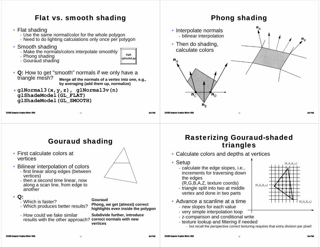
Flat vs. smooth shading• Flat shading

• Use the same normal/color for the whole polygon• Need to do lighting calculations only once per polygon

• Smooth shading• Make the normals/colors interpolate smoothly• Phong shading• Gouraud shading

• Q: How to get "smooth" normals if we only have a triangle mesh?

• glNormal3(x,y,z), glNormal3v(n)glShadeModel(GL_FLAT)glShadeModel(GL_SMOOTH)

runsphsubd.py

Merge all the normals of a vertex into one, e.g.,by averaging (add them up, normalize)


Phong shading• Interpolate normals

• bilinear interpolation

• Then do shading, calculate colors


Gouraud shading• First calculate colors at

vertices• Bilinear interpolation of colors

• first linear along edges (between vertices)

• then a second time linear, now along a scan line, from edge to another

• Q:• Which is faster?• Which produces better results?

• How could we fake similar results with the other approach?

GouraudPhong, we get (almost) correcthighlights even inside the polygonSubdivide further, introducecorrect normals with new vertices


Rasterizing Gouraud-shaded triangles

• Calculate colors and depths at vertices• Setup

• calculate the edge slopes, i.e.,increments for traversing down the edges (R,G,B,A,Z, texture coords)

• triangle split into two at middle vertex and done in two parts

• Advance a scanline at a time• new slopes for each value • very simple interpolation loop• z-comparison and conditional write• texture lookup and filtering if needed

• but recall the perspective correct texturing requires that extra division per pixel!

(R1,G1,B1,z1)

(R2,G2,B2,z2)

(R3,G3,B3,z3)


Boundaries• What is the extent of a triangle?

• need to make sure that two neighboring triangles don’t try to write on the same pixel

• Assuming you scan from bottom up• the first line of an edge is Iyenter = floor(Ybot) + 1

• the last line of an edge is Iyexit = floor(Ytop)

• Notice that with the next line (see image)• Iyenter = Iyexit + 1

• Follow the same convention with x• Ixenter = floor(Xbot) + 1• Ixexit = floor(Xtop)

(Xbot, Ybot)

(Xtop, Ytop)

Iyenter

Iyexit


Implementation• For efficient implementation, use fixed-point

calculations instead of floating point• Fixed point representation

• use some of the bits for the integer part and some for the fraction

• e.g., out of 32 bits, 12 bits for the integers, 20 for the fraction

• some of the fraction bits are for ”subpixels” into which the floating point values are quantized

• the rest are needed for accurate accumulation so that the small increments really add up

• (log2(n) bits for n accumulation steps)

• Use the same representation for both • the accumulator (the value at the pixel) and • the slope (how much the value changes when advancing)


Alternative: homogeneous rasterization

• Represent triangles with linear edge functions• like the affine coordinates, see lecture 2 page 5• positive inside the edge, negative outside

• within triangle all edge functions positive• process pixels inside the edges

• Advantage• no clipping needed!

• except for the near plane, that’s done by adding one more edge function• it’s a bit like scissoring: pixels outside the screen are just not evaluated

• cheaper processing than traditional scan conversion• fewer divisions in setup and processing

• Perspective correct interpolation required• for all parameters, such as color, in addition to texcoords• if only interpolate in screen space, clipping is must to avoid

singularities


Triangle stripping• A vertex, on the average, is adjacent to 6 triangles

• reprocessing the same vertex 6 times is wasteful

• What can you save?• lighting• projection to screen• in principle also part of triangle setup

• T-strip draws a series of triangles• v0, v1, v2; v2, v1, v3; v2, v3, v4; v4, v3, v5; …• after first triangle, process one vertex / tri, not 3 / tri• every other time flip the order of two previous vertices to

get a consistent (CCW) orientation

• Extension: vertex cache• save a lit, projected vertex in a cache• if it’s used soon again, just copy from cache

V0

V1

V2

V3

V4

V5


Hidden surfaces• Not every part of every 3D object is visible to a given viewer

• need to determine what parts of each object should get drawn

• Known as • “hidden surface elimination”• “visible surface determination”

• Important algorithms• Painter’s method + Back-face culling• Z-buffer• Scanline• Ray casting / ray tracing• List priority sorting• Binary space partitioning• Appel's edge visibility• Warnock's area subdivision


Painter’s method• The simplest method conceptually• Sort objects into back-to-front order• Do as a painter does

• first paint objects that are far away• then paint things that are closer, and they will obscure those

that are further behind

• Problem• sorting is lots of work, especially if needs to be repeated for

every frame


Back-face Culling• Can be used with polygon-based representations• Often, we don’t want to draw polygons that face away

from the viewer• so test for this and eliminate (cull) back-facing polygons

• How can we test for this?Dot the normal and direction to the viewer,if the sign is negative, the polygon is back-facing.

Faster yet is to calculate the screen area, if the area is negative, polygon is back-facing.The area of triangle ABC is half of (B-A) x (C-A) = (xb-xa)*(yc-ya) – (xc-xa)*(yb-ya).

A

BC


Back-face Culling• Commands

• glEnable( GL_CULL_FACE ) glDisable( GL_CULL_FACE )• glFrontFace( face )face = { GL_CW, GL_CCW }

• glCullFace( mode )mode = { GL_FRONT, GL_BACK, GL_FRONT_AND_BACK }

• Why both CW and CCW?• you might get data from somebody who doesn’t use CCW convention

• Why both front and back?• say you model left side of a car• you copy it for the right side, scale by –1 to mirror it• must flip which face to cull as previous inside is now outside

• For convex objects, back face culling is all that is needed!• within individual object• separate objects still need to be sorted


Z-buffer• Idea: along with a pixel’s red, green and blue values,

maintain some notion of its depth• an additional channel in memory, like alpha• called the depth buffer or Z-buffer

• For a new pixel, compare its depth with the depth already in the framebuffer, replace only if it’s closer

• Very widely used• History

• originally described as “brute-force image space algorithm”• written off as impractical algorithm for huge memories• today, done easily in hardware


Z-buffer Implementationfor p in pixels:

Z_buffer[ p ] = FARFb[ p ] = BACKGROUND_COLOUR

for P in polygons:for p in pixels_in_the_projection( P ):

# Compute depth z and shade s of P at p# both z and shade typically calculated # incrementallyz = depth( P, p )s = shade( P, p )if z < Z_buffer[ p ]:

Z_buffer[ p ] = zFb[ p ] = s


Scanline algorithm• Scan conversion without Z-

buffering!• Sort polygons by their screen y

extent• For each scanline, deal with all

active polygons• sort the polygon spans within

scanline• consider both span ends and

intersections• Only one polygon visible at a time

• visibility can change at span ends or intersections

• need to touch each pixel only once!


Ray Casting• Partition the projection plane into pixels to match

screen resolution• For each pixel pi, construct ray from COP through PP

at that pixel and into scene• Intersect the ray with every object in the scene, color

the pixel according to the object with the closest intersection


Ray Casting Implementation• Parameterize the ray:

• If a ray intersects some object Oi, get parameter tisuch that first intersection with Oi occurs at R(ti)

• Which object owns the pixel?

R(t) = (1-t)c + tpi

The one closest, with the smallest t


List Priority Sorting• Clustering

• organize the scene into linearly separable clusters• during rendering, compare depths for cluster priority• render from back to front• priority order changes when viewpoint does

• Within a cluster• each face is compared to get face priority• if a face can obscure another one, it has higher priority• can be computed once, does not change when viewpoint

does!


Face Priority• Priorities

• in figure, faces with priority 3 cannot obscure any other face

• faces with priority 2 can obscure those

• and so on

• Drawing• just draw in (inverse) priority

order• use back face culling• in the example, draw only

two faces (all others back facing), first 2 and then 1

1 1

1

1

22

3

3

1

2


Binary Space Partitioning• Goal: build a tree that captures some relative depth

information between objects, use it to draw objects in the right order

• tree doesn’t depend on camera position, so we can change viewpoint and redraw quickly

• called the binary space partitioning tree, or BSP tree

• Key observation: The polygons in the scene are painted in the correct order if for each polygon P,

• polygons on the far side of P are painted first• P is painted next• polygons in front of P are painted last


Building a BSP Tree (in 2D)


BSP Tree Construction

• Splitting polygons is expensive! It helps to choose P wisely at each step

• Example: choose five candidates, keep the one that splits the fewest polygons

def makeBSP(L): # L: list of polygonsif not L:

return None# Choose a polygon P from L to serve as rootP = get_root(L)# Split all polygons in L according to Pneg_side_polys, pos_side_polys = split(P, L)return TreeNode(P,

makeBSP( neg_side_polys ),makeBSP( pos_side_polys ))


BSP Tree Displaydef showBSP( viewer, BSPtree ):

if not BSPtree:return

P = BSPtree.rootif P.in_front_of(viewer):

showBSP( BSPtree.left_subtree )draw( P )showBSP( BSPtree.right_subtree )

else:showBSP( BSPtree.right_subtree )draw( P )showBSP( BSPtree.left_subtree )


Appel's visible line algorithm• Calculate quantitative

invisibility of a point• how many faces occlude a point?• when a line passes behind a front-

facing polygon, increase by 1• when it passes out from behind,

decrease by 1• line visible = quant.inv. is 0

• Changes at a contour line• edge shared by a front- and back-

facing polygon• unshared front-facing edge• are: AB, CD, DF, KL• not: CE, EF, JK


Appel's visible line algorithm• First get a "seed"

• e.g., the closest vertex or brute force calculation

• Propagate the value along edges

• until the next vertex• or intersection• then recalculate the number

• At some vertices the adjacent edges’ quantitative invisibility may differ

• an incident face may hide an edge• KJ = 0• KL = 1


Warnock's algorithm• Recursively subdivide into

four squares• Try to obtain a simple

solution at the smaller square

• Potentially go down to pixel level


Warnock's algorithm

• Four cases:• surrounding polygon contains the area• intersecting polygons• contained polygons• disjoint polygons


Warnock's cases• Only disjoint polygons

• paint with background color

• Only one intersecting or contained polygon• paint with background, scan convert polygon

• Single surrounding polygon• paint with polygon's color

• Otherwise• if one surrounding is

in front, paint• else subdivide


An alternative splitting scheme• Split at vertices

• instead of at predetermined spots

• Need fewer splits


Analysis of HS methods


Object vs. Image Space• Object space

• operate on geometric primitives (3D), asks whether each potentially visible thing is visible

• for each object in the scene, compute the part of it which isn’t obscured by any other object, then draw

• must perform tests at high precision, results are resolution-independent

• Image space• operate on pixels (2D), asks what is visible within a pixel • for each pixel, find the object closest to the COP which

intersects the projector through that pixel, then draw• tests at device resolution, result works only for that

resolution


Object vs. Image Order• Object order

• consider each object only once - draw its pixels and move on to the next object

• might draw the same pixel multiple times

• Image order• consider each pixel only once - draw part of an object and

move on to the next pixel• might compute relationships between objects multiple times


Sort First vs. Sort Last• Sort first

• first sort to find some depth-based ordering of the objects relative to the camera, then draw from back to front

• build an ordered data structure to avoid duplicating work

• Sort last• start drawing even before everything has been sorted, sort

implicitly as more information becomes available


Some additional definitions• An algorithm exhibits coherence if it uses knowledge

about the continuity of the objects on which it operates

• using coherence can greatly accelerate an algorithm• area coherence, frame-to-frame coherence, …

• An online algorithm is one that doesn’t need all the data to be present when it starts running

• Example: insertion sort

• A cycle• a sequence of objects for which you cannot

define a unique front-to-back ordering

• A self-intersection


Methods analyzed

noyes (intersections)yesyesno (but can

be faster)yesnoyespre-

processing

nonononononoyesnoonline

transp

painter’s: anything

bfcull: yes

no

first

obj

obj

painter’s + bf-cull

transp

anything

yes

first

img

img

scanline

yes

anything

yes

last

img

img

raytrace

nonotransptransptransptransparency / refraction

not necessarily

yesyesyesusuallypolygon-based

yescyclesyes (with splitting)

noyescycles / self-intersections

lastlastfirstfirstlastsort

imgobjobjobjobjorder

imgobjobjobjimgspace

WarnockAppelBSPlist priority

z-buf

scan converting lines line equation algorithmpang/160/f12/slides/dda.pdfscan converting lines •...

Documents