United StatesDepartmentof Agriculture

Forest Service

Rocky MountainForest and RangeExperiment Station

Fort Collins,Colorado 80526

Research PaperRM-293

Scaling of Ratings:

Concepts and Methods

Thomas C. BrownTerry C. Daniel

This file was created by scanning the printed publication.Errors identified by the software have been corrected;

however, some errors may remain.

Abstract

Rating scales provide an efficient and widely used means of recordingjudgments. This paper reviews scaling issues within the context of apsychometric model of the rating process and describes several meth-ods of scaling rating data. The scaling procedures include the simplemean, standardized values, scale values based on Thurstone’s Law ofCategorical Judgment, and regression-based values. The scaling meth-ods are compared in terms of the assumptions they require about therating process and the information they provide about the underlyingpsychological dimension being assessed.

Acknowledgments

The authors thank R. Bruce Hull, Howard E. A. Tinsley, Gregory J.Buhyoff, A. J. Figueredo, Rudy King, Joanne Vining, and Paul Gobster foruseful comments.

USDA Forest Service September 1990Research Paper RM-293

Scaling of Ratings: Concepts and MethodsThomas C. Brown, Economist

Rocky Mountain Forest and Range Experiment Station1

Terry C. Daniel, ProfessorDepartment of Psychology, University of Arizona

1Headquarters is at 240 W. Prospect Street, Fort Collins, CO 80526, in cooperation with Colorado State University.

Contents

Page

INTRODUCTION ......................................................................................................... 1

PSYCHOLOGICAL SCALING ..................................................................................... 1

Scaling Levels ......................................................................................................... 1

Scaling Methods ..................................................................................................... 2

Rating Scales .......................................................................................................... 3

Psychometric Model........................................................................................... 3

Problems With Interpreting Rating Scales ....................................................... 4

Baseline Adjustments ............................................................................................ 6

SCALING PROCEDURES ........................................................................................... 6

Median Rating ......................................................................................................... 7

Mean Rating ............................................................................................................ 7

Origin-Adjusted Rating........................................................................................... 8

Baseline-Adjusted OAR ...................................................................................... 8

Z-Score .................................................................................................................... 8

Baseline-Adjusted Z-Score .............................................................................. 10

Least Squares Rating ........................................................................................... 10

Baseline-Adjusted LSR ..................................................................................... 12

Comparison of Z-Scores and LSRs ................................................................. 12

Scenic Beauty Estimate ....................................................................................... 13

By-Stimulus SBE ................................................................................................ 15

By-Observer SBE ............................................................................................... 16

Comparison of By-Stimulus and By-Observer SBEs ..................................... 17

Comparison of SBEs and Mean Ratings ......................................................... 17

Comparison of SBEs With Z-Scores and LSRs .............................................. 18

Summary ............................................................................................................... 18

Scaling Procedures and the Interpretation of Ratings .................................. 18

Which Procedure To Use When..................................................................... 19

LITERATURE CITED ................................................................................................. 20

APPENDIX: RELATIONSHIPS AMONG SCALE VALUES ....................................... 21

1

INTRODUCTION

Rating scales offer an efficient and widely used means of

recording judgments about many kinds of stimuli. Suchscales are often used in studies relating to natural re-

sources management, for example, to measure citizen

preferences for recreation activities (Driver and Knopf1977) or perceived scenic beauty of forest scenes (Brown

and Daniel 1986). In this paper we review issues regarding

the use of rating data, and describe and compare methodsfor scaling such data.

This paper provides theoretical and descriptive back-

ground for scaling procedures available in a computerprogram called RMRATE, which is described in a compan-

ion document (Brown et al. 1990). RMRATE is designed to

(1) scale rating data using a battery of scaling procedures,(2) compare the scale values obtained by use of these

procedures, (3) evaluate to a limited extent whether the

assumptions of the scaling procedures are tenable, (4) de-termine the reliability of the ratings, and (5) evaluate indi-

vidual variations among raters.

Both this paper and the RMRATE computer program areoutgrowths of an effort that began in the early 1970s to

better understand the effects of management on the sce-

nic beauty of forest environments. An important report byDaniel and Boster (1976) introduced the Scenic Beauty

Estimation (SBE) method. The SBE method is reviewed

and further developed herein, along with other scalingprocedures, including median and mean ratings, stan-

dardized scores, and a new scale based on a least squares

analysis of the ratings.While scenic beauty has been the focus of the work that

led up to this paper, and continues to be a major research

emphasis of the authors, the utility of the scaling proce-dures is certainly not limited to measurement of scenic

beauty. Rather, this paper should be of interest to anyone

planning to obtain or needing to analyze ratings, no matterwhat the stimuli.

Psychological scaling procedures are designed to deal

with the quite likely possibility that people will use therating scale differently from one to another in the process

of recording their perceptions of the stimuli presented for

assessment. Scaling procedures can be very effective inadjusting for some of these differences, but the proce-

dures cannot correct for basic flaws in experimental de-

sign that are also reflected in the ratings. While aspects ofexperimental design are mentioned throughout this paper,

we will not cover experimental design in detail; the reader

desiring an explicit treatment of experimental design shouldconsult a basic text on the topic, such as Cochran and Cox

(1957) or Campbell and Stanley (1963).

We first offer a brief introduction to psychological scal-ing to refresh the reader’s memory and set the stage for

what follows. Readers with no prior knowledge of scaling

Scaling of Ratings: Concepts and MethodsThomas C. Brown and Terry C. Daniel

methods should consult a basic text on the subject, such as

Nunnally (1978) or Torgerson (1958). We then describe

and compare several procedures for scaling rating data.Finally, additional comparisons of the scaling procedures

are found in the appendix.

PSYCHOLOGICAL SCALING

Psychometricians and psychophysicists have developed

scaling procedures for assigning numbers to the psycho-

logical properties of persons and objects. Psychometri-cians have traditionally concentrated on developing mea-

sures of psychological characteristics or traits of persons,

such as the IQ measure of intelligence. Psychophysics isconcerned with obtaining systematic measures of psycho-

logical response to physical properties of objects or envi-

ronments. A classic example of a psychophysical scale isthe decibel scale of perceived loudness.

Among the areas of study to which psychophysical meth-

ods have been applied, and one that is a primary area ofapplication for RMRATE (Brown et al. 1990), is the scaling

of perceived environmental quality and preferences. In

this context, scaling methods are applied to measure dif-ferences among environmental settings on psychological

dimensions such as esthetic quality, scenic beauty, per-

ceived naturalness, recreational quality, or preference.

Scaling Levels

An important consideration in psychological scaling, as

in all measurement, is the “level” of the scale that isachieved. Classically there are three levels that are distin-

guished by the relationship between the numbers derived

by the scale and the underlying property of the objects (orpersons) that are being measured. The lowest level of

measurement we will discuss is the ordinal level, where

objects are simply ranked, as from low to high, with re-spect to the underlying property of interest. At this level, a

higher number on the scale implies a higher degree (greater

amount) of the property measured, but the magnitude ofthe differences between objects is not determined. Thus,

a rank of 3 is below that of 4, and 4 is below 6, but the scale

does not provide information as to whether the object atrank 4 differs more from the object at 3 or from the object

ranked at 6. At this level of measurement only statements

of “less than,” “equal to,” or “greater than,” with respect tothe underlying property, can be supported.

Most psychological scaling methods seek to achieve an

interval level of measurement, where the magnitude ofthe difference between scale values indicates, for ex-

ample, the extent to which one object is preferred over

another. The intervals of this metric are comparable over

2

the range of the scale; e.g., the difference between scale

values of 1 and 5 is equivalent to the difference between 11and 15 with respect to the underlying property. Interval

scale metrics have an arbitrary zero point, or a “rational”

origin (such as the Celsius scale of temperature where 0degrees is defined by the freezing point of water). They do

not, however, have a true zero point that indicates the

complete absence of the property being measured.Interval scales will support mathematical statements

about the magnitude of differences between objects with

respect to the property being measured. For example, astatement such as “a difference of 4 units on the measure-

ment scale represents twice as great a difference in the

underlying property as a difference of 2 units” could bemade about information in an interval scale. It would not

be permissible, however, to state that “the object with a

value of 4 has twice as much of the property being mea-sured as the object scaled at 2.” The latter statement

requires a higher level of measurement, one where all

scale values are referenced to an “absolute zero.”The highest level of measurement is the ratio scale,

where the ratios of differences are equal over the range of

the scale; e.g., a scale value of 1 is to 2 as 10 is to 20. Ratioscales require a “true zero” or “absolute” origin, where 0

on the scale represents the complete absence of the prop-

erty being measured (such as the Kelvin scale of tempera-ture, where 0 represents the complete absence of heat).

Generally, ratio scales are only achieved in basic physical

measurement systems, such as length and weight. Abso-lute zeros are much harder to define in psychological

measurement systems, because of the difficulty of deter-

mining what would constitute the absolute absence ofcharacteristics such as intelligence or preference.

It is important to note that the ordinal, interval, or ratio

property of a measurement scale is determined with refer-ence to the underlying dimension being measured; 20

degrees Celsius is certainly twice as many degrees as 10,

but it does not necessarily represent twice as much heat.The level of measurement may place restrictions on the

validity of inferences that can be drawn about the underly-

ing property being measured based on operations per-formed on the scale values (the numbers). Some fre-

quently used mathematical operations, such as the

computation and comparison of averages, require assump-tions that are not met by some measurement scales. In

particular, if the average of scale values is to represent an

average of the underlying property, then the measurementscale must be at least at the interval level, where equal

distances on the measurement scale indicate equal differ-

ences in the underlying property. Similarly, if ratios of scalevalues are computed, only a ratio scale will reflect equiva-

lent ratios in the underlying property.

Scaling Methods

A number of different methods can be used for psycho-logical scaling. All methods involve the presentation of

objects to observers who must give some overt indication

of the relative position of the objects on some desig-

nated psychological dimension (e.g., perceived weight,brightness, or preference). Traditional methods for ob-

taining reactions to the objects in a scaling experiment

include paired-comparisons, rank orderings, and nu-merical ratings.

Perhaps the simplest psychophysical measurement

method conceptually is the method of paired compari-sons. Objects are presented to observers two at a time, and

the observer is required to indicate which has the higher

value on the underlying scale; e.g., in the case of prefer-ences, the observer indicates which of the two is most

preferred. A related procedure is the rank-order proce-

dure. Here the observer places a relatively small set ofobjects (rarely more than 10) in order from lowest (least

preferred) to highest (most preferred). At their most basic

level, these two procedures produce ordinal data, basedon the proportion of times each stimulus is preferred in the

paired-comparison case, and on the assigned ranks in the

rank-ordering procedure.One of the most popular methods for obtaining reactions

from observers in a psychological measurement context

uses rating scales. The procedure requires observers toassign ratings to objects to indicate their attitude about

some statement or object, or their perception of some

property of the object.In each of these methods, the overt responses of the

observers (choices, ranks, or ratings) are not taken as direct

measures of the psychological scale values, but are used asindicators from which estimates of the psychological scale

are derived using mathematical procedures appropriate to

the method. In theory, the psychological scale values de-rived for a set of objects should not differ between different

scaling methods. For example, if a paired-comparison pro-

cedure and a rating scale are used for indicating relativepreferences for a common set of objects, the psychological

preference scale values for the objects should be the same,

or within a linear transformation.While the basic data from the paired-comparison and

rank-order procedures are originally at the ordinal level of

measurement, psychometric scaling procedures have beendeveloped that, given certain theoretical assumptions,

provide interval level measures. Perhaps the best known

procedures are those developed by Thurstone (seeNunnally (1978) and Torgerson (1958)), whereby choices

or ranks provided by a number of observers (or by one

observer on repeated occasions) are aggregated to obtainpercentiles, which are then referenced to a normal distri-

bution to produce interval scale values for the objects

being judged. A related set of methods, also based onnormal distribution assumptions, was developed for rating

scale data. Later sections of this paper describe and com-

pare procedures used with rating data. Additional, moredetailed presentations of the theoretical rationale and the

computational procedures are found in the texts by au-

thors such as Torgerson (1958) and Nunnally (1978). Dis-cussion of these issues in the context of landscape prefer-

ence assessment can be found in papers by Daniel and

Boster (1976), Buhyoff et al. (1981), and Hull et al. (1984).

3

Rating Scales

Rating response scales are typically used in one of twoways. With the first approach, each value of the rating

scale can carry a specific descriptor. This procedure is

often used in attitude assessment. For example, the valuesof a 5-point scale could be specified as (1) completely

agree, (2) tend to agree, (3) indifferent, (4) tend to dis-

agree, and (5) completely disagree, where the observer isto indicate degree of agreement about a set of statements.

The observer chooses the number of the response that

most closely represents his/her attitude about each state-ment. With the second use of rating scales, only the end-

points of the scale are specified. This format is commonly

used with environmental stimuli, where observers arerequired to assign ratings to stimuli to indicate their per-

ception of some property of the stimuli. “very low prefer-

ence” for the stimulus, and a “10” indicating very highpreference.” Ratings between 1 and 10 are to indicate

levels of preference between the two extremes. The end-

points are specified to indicate the direction of the scale(e.g., low ratings for less preference, high ratings for more

preference).

Whether associated with a specific descriptor or not, anindividual rating, by itself, cannot be taken as an indicator

of any particular (absolute) value on the underlying scale.

For example, labeling one of the categories “strongly agree”in no way assures that “strong” agreement in one assess-

ment context is equivalent to “strong” agreement in an-

other. Similarly, a rating of “5” by itself provides no infor-mation. A given rating provides useful information only

when it is compared with another rating; that is, there is

meaning only in the relationships among ratings as indica-tors of the property being assessed. Thus, it is informative

to know that one stimulus is rated a 5 when a second

stimulus is rated a 6. Here the ratings indicate whichstimulus is perceived to have more of the property being

assessed. Furthermore, if a third stimulus is rated an 8, we

may have information not only about the ranking of thestimuli, but also about the degree to which the stimuli are

perceived to differ in the property being assessed.

Ratings, at a minimum, provide ordinal-level informa-tion about the stimuli on the underlying dimension being

assessed. However, ratings are subject to several potential

“problems” which, to the extent they exist, tend to limit thedegree to which rating data provide interval scale informa-

tion and the degree to which ratings of different observers

are comparable. Before we review some of these prob-lems, it will be useful to present a model of the process by

which ratings are formed and scaled.

Psychometric Model

The objective of a rating exercise is to obtain a numerical

indication of observers’ perceptions of the relative posi-

tion of one stimulus versus another on a specified psycho-logical dimension (e.g., scenic beauty). This objective is

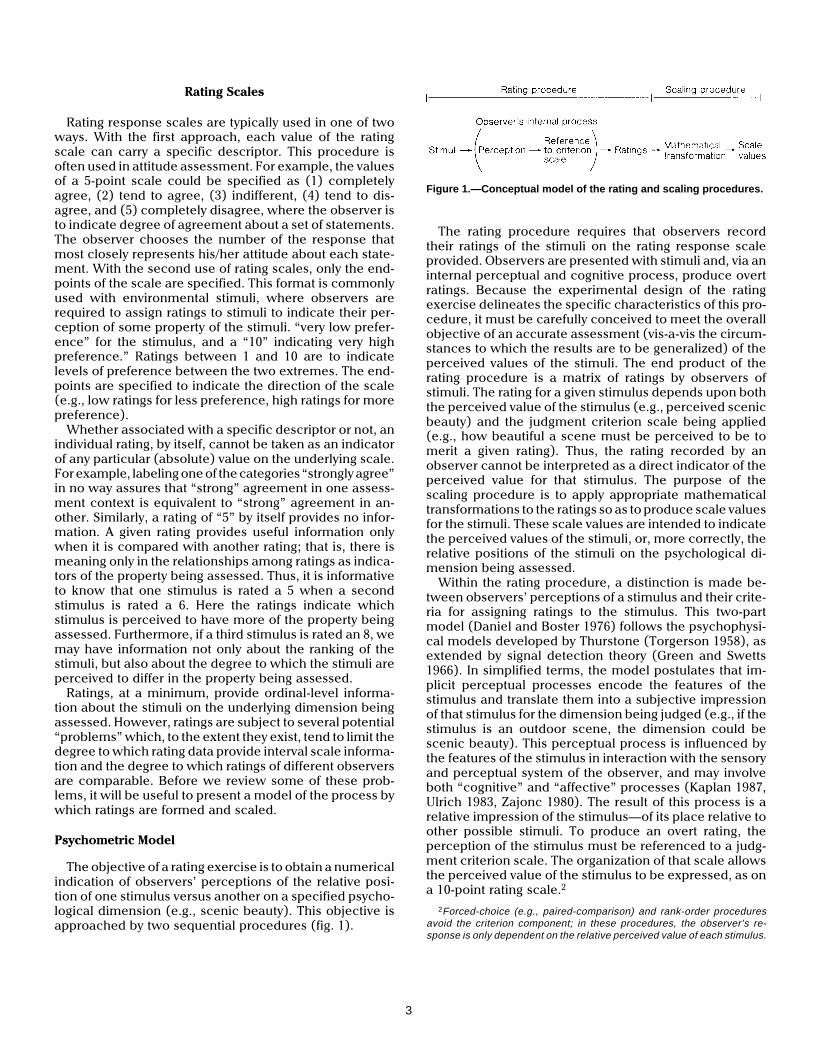
approached by two sequential procedures (fig. 1).

Figure 1.—Conceptual model of the rating and scaling procedures.

The rating procedure requires that observers record

their ratings of the stimuli on the rating response scaleprovided. Observers are presented with stimuli and, via an

internal perceptual and cognitive process, produce overt

ratings. Because the experimental design of the ratingexercise delineates the specific characteristics of this pro-

cedure, it must be carefully conceived to meet the overall

objective of an accurate assessment (vis-a-vis the circum-stances to which the results are to be generalized) of the

perceived values of the stimuli. The end product of the

rating procedure is a matrix of ratings by observers ofstimuli. The rating for a given stimulus depends upon both

the perceived value of the stimulus (e.g., perceived scenic

beauty) and the judgment criterion scale being applied(e.g., how beautiful a scene must be perceived to be to

merit a given rating). Thus, the rating recorded by an

observer cannot be interpreted as a direct indicator of theperceived value for that stimulus. The purpose of the

scaling procedure is to apply appropriate mathematical

transformations to the ratings so as to produce scale valuesfor the stimuli. These scale values are intended to indicate

the perceived values of the stimuli, or, more correctly, the

relative positions of the stimuli on the psychological di-mension being assessed.

Within the rating procedure, a distinction is made be-

tween observers’ perceptions of a stimulus and their crite-ria for assigning ratings to the stimulus. This two-part

model (Daniel and Boster 1976) follows the psychophysi-

cal models developed by Thurstone (Torgerson 1958), asextended by signal detection theory (Green and Swetts

1966). In simplified terms, the model postulates that im-

plicit perceptual processes encode the features of thestimulus and translate them into a subjective impression

of that stimulus for the dimension being judged (e.g., if the

stimulus is an outdoor scene, the dimension could bescenic beauty). This perceptual process is influenced by

the features of the stimulus in interaction with the sensory

and perceptual system of the observer, and may involveboth “cognitive” and “affective” processes (Kaplan 1987,

Ulrich 1983, Zajonc 1980). The result of this process is a

relative impression of the stimulus—of its place relative toother possible stimuli. To produce an overt rating, the

perception of the stimulus must be referenced to a judg-

ment criterion scale. The organization of that scale allowsthe perceived value of the stimulus to be expressed, as on

a 10-point rating scale.2

2Forced-choice (e.g., paired-comparison) and rank-order proceduresavoid the criterion component; in these procedures, the observer’s re-sponse is only dependent on the relative perceived value of each stimulus.

4

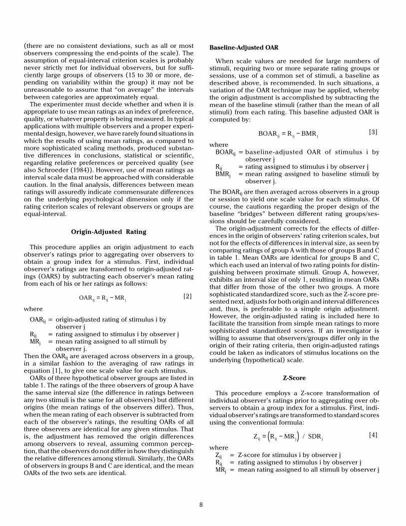
Figure 2 depicts how hypothetical perceived values for

each of three stimuli could produce overt ratings accord-ing to four different observers’ judgment criterion scales.

For this example the perceived values for the three stimuli

are assumed to be identical for all four observers, and areindicated by the three horizontal lines that pass from the

“perceived value” axis through the four different judgment

criterion scales. When referred to the judgment criterionscale of observer A, the perceived value of stimulus 1 is

sufficient to meet the criterion for the eighth category, but

not high enough to reach the ninth category, so the ob-server would assign a rating of 8 to the stimulus. Similarly,

the same stimulus would be assigned a rating of 10 accord-

ing to observer C’s judgment criterion scale, and only a 6according to observer D’s judgment criterion scale.

The illustration in figure 2 begins with the assumption

that the four observers have identical perceptions of thestimuli, but different judgment criterion scales. In actual

applications, of course, neither the perceived values nor

the criterion scales are known; only the overt ratings areavailable for analysis. However, guided by a psychometric

model, scaling procedures derive estimates of differences

in perceived values that are potentially independent ofdifferences in judgment criteria. Relationships between

ratings of different stimuli by the same observer(s) are

used to infer perceptions. Given the conditions illustratedin figure 2, where only observer rating criteria differ, the

ideal scaling procedure would translate each observer’s

ratings so that the scale values for a given stimulus wouldbe identical for all four observers.

Problems With Interpreting Rating Scales

Unequal-interval judgment criterion scales.—The ratingscale provides an opportunity for observers to directly

indicate magnitudes of differences in their perceptions of

the objects, which is not provided by either paired-com-parison or rank-order techniques. However, for this to

occur, the intervals between rating categories must be

equal with regard to the underlying property being mea-sured. Equally spaced intervals would require that, for

example, the difference in the dimension being rated

yielding an increase in rating from 2 to 3 is equal to thedifference in that dimension yielding an increase in rating

from 6 to 7. The criterion scales of observers B, C, and D of

figure 2 are equal-interval scales, while the scale of ob-server A is an unequal-interval scale.

Unfortunately, the intervals between rating categories

on the underlying psychological dimension will not neces-sarily be equal. An obvious potential cause of unequal

intervals in people’s use of the rating scale is the “end-

point” problem. This problem could arise when an ob-server encounters a stimulus to be rated that does not fit

within the rating criteria that the observer has established

in the course of rating previous stimuli. For example, theobserver may encounter a stimulus that he/she perceives

to have considerably less of the property being rated than

a previous stimulus that was assigned the lowest possiblerating. This new stimulus will also be assigned the lowest

possible rating, which may result in a greater range of the

property being assigned to the lowest rating category thanto other rating categories. This may occur at both ends of

the rating scale, resulting in a sigmoid type relationship

between ratings and the underlying property (Edwards1957).

The end-point problem can be ameliorated by showing

observers a set of “preview” stimuli that depicts the rangeof stimuli subsequently to be rated. This allows observers

to set (“anchor”) their rating criteria to encompass the full

range of the property to be encountered during the ratingsession. Hull et al. (1984) used this procedure when they

compared rating scale values to paired-comparison scale

values for the same stimuli. Paired-comparisons, of course,are not subject to an endpoint constriction. The linear

relationship they found between the two sets of scale

values extended to the ends of the scale, suggesting thatthe ratings they obtained did not suffer from the end-point

problem.

Of course, the end-point problem is not the only poten-tial source of unequal-interval ratings. Observers are free

to adopt any standards they wish for assigning their ratings,

and there is no a priori reason to expect that they will useequal intervals. For example, the intervals might gradually

get larger the farther they are from the center of the scale,

as in the criterion scale of observer A in figure 2.Because it is not possible to directly test for equality of

intervals among an observer’s ratings, some statisticians

argue that ratings should not be used as if they representinterval data (e.g., Golbeck 1986). Others, however, argue,

based on Monte Carlo simulations and other approaches,

that there is little risk in applying parametric statistics torating data, especially if ratings from a sufficient number of

observers are being combined (Baker et al. 1966, Gregoire

and Driver 1987, O’Brien 1979). Nevertheless, the possibilityof an unequal-interval scale leaves the level of measurementFigure 2.—Judgment criterion scales of four observers with identical

perceived values.

5

achieved by rating scales somewhat ambiguous. The criti-

cal issue, of course, is how the ratings, and any statistics orindices computed from those ratings, relate to the under-

lying (psychological) dimension that is being assessed.

This issue can only be addressed in the context of sometheory or psychometric model of the perceptual/judgmen-

tal process.

Lack of interobserver correspondence.—Individualobserver’s ratings frequently do not agree with those of

other observers for the same stimuli. Lack of correspon-

dence could result from differences in perception, whichof course is not a “problem” at all; rather it is simply a

finding of the rating exercise at hand. Lack of correspon-

dence could also result from poor understanding of therating task, poor eyesight or other sensory malfunction,

simple observer distraction, or even intentional misrepre-

sentation. Principal component analysis or cluster analysistechniques may be useful to determine whether observers

fall into distinct groups with regard to their perception of

the stimuli, or whether observers who disagree are unique.In some cases it may be appropriate to either drop some

observers from the sample (as being unrepresentative of

the population of interest) or weight their ratings less thanothers.

Most often, lack of correspondence between observers

will be due to differences in the judgment (rating) criteriaadopted. Even if individual observers each employ equal-

interval rating criteria, criterion scales can vary between

observers, or the same observer may change criteria fromone rating session to another. As a consequence, ratings

can differ even though the perception of the stimuli is the

same (as shown in fig. 2). When differences betweenobservers’ ratings are due only to differences in the crite-

rion scale (i.e., their perceived values are the same), their

resulting ratings will be monotonically related, but notnecessarily perfectly correlated. But if these observers

employ equal-interval criterion scales, the resulting rat-

ings will also be perfectly correlated (except for randomvariation).

Linear differences in ratings consist of “origin” and

“interval size” components. Assuming equal-intervalscales, these two components can be estimated for two

sets of ratings of the same stimuli by simply regressing

one set on the other. The intercept and slope coefficientsof the regression would indicate the origin and interval

size differences, respectively. As an example of an origin

difference, consider criterion scales of observers B and Cin figure 2. Remember that all observers in figure 2 are

assumed to agree in their perception of the stimuli. Ob-

server B’s and C’s criterion scales have identical intervalsizes, but B’s scale is shifted up two rating values com-

pared with C’s scale (suggesting that observer B adopted

more stringent criteria, setting higher standards than ob-server C). The ratings of these two observers for scenes 1,

2, and 3 can be made identical by a simple origin shift—

either adding “2” to each of B’s ratings or subtracting “2”from each of C’s ratings.

Observers’ criterion scales can probably be expected to

differ somewhat by both their origin and interval size. Asan example, consider the criterion scales of observers C

and D in figure 2. The judgments for the three stimuli

(ratings of 4, 7, and 10 for observer C and 2, 4, and 6 forobserver D) indicate that these scales differ by an origin

shift of 1.0 and an interval size of 1.5. That is, the relation-

ship between the ratings of observers C and D is repre-sented by RC = 1 + 1.5 RD, where RC, and RD indicate the

ratings of observers C and D, respectively.

There is no direct way to observe either the perceivedvalues of the stimuli or the judgment criteria used by the

observer; both are implicit psychological processes. Thus,

if two sets of ratings are linearly related, it is impossible totell for sure whether the ratings were produced (1) by two

observers who have identical rating criterion scales, but

perceive the stimuli differently; (2) by two observers whoperceive the stimuli the same, but use different criterion

scales; or (3) by two observers who differ both in percep-

tion and rating criteria. In our application of the basicpsychometric model, however, we have taken the position

that perception is a relatively consistent process that is

strongly related to the features of the stimulus, whilejudgment (rating) criteria are more susceptible to the

effects of personal, social, and situational factors. This is a

theoretical position that is consistent with the Thurstoneand signal detection theory models (Brown and Daniel

1987, Daniel and Boster 1976, Hays 1969). Given this posi-

tion, linear differences (i.e., differences in origin and inter-val size) between sets of ratings are generally taken to be

indications of differences in judgment criteria, not differ-

ences in perception. When differences in ratings are dueto the criterion scales used by different observers (or

observer groups), psychometric scaling procedures can

adjust for these effects and provide “truer” estimates of theperceived values of the stimuli.

Linear differences between group average criterionscales.—A related problem may arise where ratings of twodifferent observer groups are to be compared. The two

groups may on average use different rating criteria, per-

haps because of situational factors such as when the ratingsessions of the different groups occurred. For example,

time of day may influence ratings, regardless of the spe-

cific attributes of the stimuli being judged. Scaling proce-dures can be used to adjust for criterion differences (origin

and interval) between observer groups.

Lack of intraobserver consistency.—An individualobserver’s ratings can be inconsistent, with different rat-

ings being assigned to the same stimulus at different times.

This problem is not restricted to ratings, but can occurwhenever an observer’s perception and/or rating criterion

boundaries waver during the rating exercise, so that, for

example, a given stimulus falls in the “6” category on oneoccasion and in the “5” category the next.

Psychometric models generally assume that both the

perceived values and the judgment criteria will vary some-what from moment to moment for any given stimulus/

observer. This variation is assumed to occur because of

random (error) factors, and thus is expected to yield anormal distribution of perceived criterion values cen-

tered around the “true” values (Torgerson 1958). Given

these assumptions, the mean of the resulting ratings for astimulus indicates the “true value” for that stimulus,

6

and the variance of the observer’s ratings for that stimulus

indicates the variation in underlying perceived values com-bined with variation in rating criterion boundaries. The

effects of inconsistencies in an observer’s ratings can be

ameliorated by obtaining a sufficient number of judgmentsof each stimulus (by requiring each observer to judge each

stimulus several times) to achieve a stable estimate of the

perceived values. Repeated presentation of the samestimuli may, however, lead to other problems.

Perceptual and criterion shifts.—In some circumstances

there may be a systematic shift in rating criteria and/orperception over the course of a rating session. Such a shift

could be related to the order in which the stimuli are

presented, or to other aspects of the rating session.3 This isa potential problem with all types of observer judgments

where several stimuli are judged by each observer. If the

problem is related to order of presentation, it can becontrolled for by presenting the stimuli to different observ-

ers (or on different occasions) in different random orders.

If the shift is primarily, due to changing criteria, it may bepossible to adjust for this effect to reveal more consistent

perceived values.

Baseline Adjustments

It is often necessary to combine the ratings for a set ofstimuli obtained in one rating session with ratings for

another set of stimuli obtained in a different rating session

(for examples, see Brown and Daniel (1984) and Danieland Boster (1976)). This need may occur, for example,

when ratings are needed for a large group of stimuli that

cannot all be rated in the same session. In such cases, theinvestigator’s option is to divide the set of stimuli into

smaller sets to be rated by different observer groups, or by

the same group in separate sessions. In either case, it isimportant that some stimuli are common to the separate

groups/sessions; this provides a basis for determining the

comparability of the ratings obtained from the differentgroups/sessions, and possibly a vehicle to “bridge the gap”

between different groups/sessions. The subset of stimuli

common to all rating sessions is called the baseline.If baseline stimuli are to be used to determine compara-

bility between two or more rating sessions, it is important

that the baseline stimuli be rated under the same circum-stances in each case. Otherwise, the ratings may be influ-

enced by unwanted experimental artifacts, such as inter-

actions between the baseline stimuli and the other stimulithat are unique to each session. To enhance the utility of

baseline stimuli, the following precautions should be fol-

lowed: (1) the observers for each session should be ran-domly selected from the same observer population, (2) the

observer groups should be sufficiently large, (3) the baseline

stimuli should be representative of the full set of stimuli tobe rated, (4) the other (nonbaseline) stimuli should be

randomly assigned to the different sessions4, and (5) all

other aspects of the sessions (e.g., time of day, experi-menter) should remain constant.

The effectiveness of a baseline is also a function of the

number of stimuli included in the baseline. The greater theproportion of the stimuli to be rated that are baseline

stimuli, the more likely that the baseline will adequately

pick up differences in use of the rating scale betweenobservers or observer groups, all else being equal. Of

course, one must trade off effectiveness of the baseline

with the decrease in the number of unique stimuli that canbe rated in each session as the baseline becomes larger.

If proper experimental precautions are followed, it is

unlikely that the ratings will reflect substantial perceptualdifferences among the different groups/sessions. In this

case, given the model described above, we would assume

that any differences across sessions in baseline ratingswere due to differences in judgment criteria, not differ-

ences in perception, and we would then proceed to use

the baseline ratings to “bridge the gap” between the ratingsessions.

In the following section, we describe and compare 11

methods for scaling rating data. Some of these proceduresattempt to compensate or adjust for the potential prob-

lems described above, and some utilize a baseline. We do

not attempt to determine the relative merit of these proce-dures. Our purpose is to provide the reader with the means

to evaluate the utility of the various scaling procedures for

any given application.

SCALING PROCEDURES

Eleven scaling procedures are described, from the simple

median and mean to the more complex Scenic Beauty

Estimation (SBE) and least squares techniques. All 11procedures are provided by RMRATE (Brown et al. 1990).

All but one of the scaling procedures provide a scale value

for each stimulus, and all procedures provide scale valuesfor groups of stimuli. In addition, some of the procedures

provide scale values for each rating. The scaling options

are described below, along with some discussion of therelative advantages and disadvantages of each.

Differences among the various scaling methods are

illustrated using several sets of hypothetical rating data.Each set of data represents ratings of the same five

stimuli by different groups of observers. For example,

table 1 presents the ratings of three hypothetical observergroups (A, B, and C) each rating the same five stimuli

3An example of such shifts is found in the “context” study reported byBrown and Daniel (1987). Two observer groups each rated the scenicbeauty of a set of common landscape scenes after they had rated a set ofunique (to the groups) scenes. Because of the differences between the twosets of unique scenes, the ratings of the initial common scenes were quitedifferent between the groups. However, as more common scenes wererated, the groups’ ratings gradually shifted toward consensus.

4An example of where this guideline was not followed is reported byBrown and Daniel (1987), where mean scenic beauty ratings for a constantset of landscape scenes were significantly different depending upon therelative scenic beauty of other scenes presented along with the constant(baseline) scenes. In that study, the experimental design was tailoredprecisely to encourage, not avoid, differences in rating criteria by differentobserver groups.

7

(1, 2, 3, 4, and 5). Table 1 provides a comparison of simple

mean ratings and baseline-adjusted mean ratings as scal-ing options. Subsequent tables use some of the same

rating sets (observer groups), as well as additional hypo-

thetical groups, to compare the other scaling options.Additional comparisons of the scaling procedures are pre-

sented in the appendix.

Median Rating

The scale value calculated using this procedure repre-sents the numerical rating that is above the ratings as-

signed by one-half of the observers and below the ratings

assigned by the other half of the observers. Thus, themedian is simply the midpoint rating in the set of ordered

ratings; e.g., among the ratings 3, 6, and 2, the median is 3.

If there is an even number of observers, the median is theaverage of the two midpoint ratings; e.g., among the rat-

ings 2, 4, 5, and 6, the median is 4.5. If the ratings assigned

to a stimulus are symmetrically (e.g., normally) distrib-uted, the median is equal to the mean rating.

An advantage of the median is that it does not require the

assumption of equal-interval ratings. The correspondingdisadvantage is that it provides only an ordinal (rank-

order) scaling. In terms of the psychological model pre-

sented above, selecting the median ratings as the scalevalue restricts one to simple ordinal (greater than, less

than) information about the position of stimuli on the

underlying psychological dimension (e.g., perceivedbeauty).

Mean Rating

In many applications researchers have used simple av-

erage ratings as a scale value. The mean rating for astimulus is computed as:

MRn

Ri ijj 1

n

==∑1 [1]

where

MRi = mean rating assigned to stimulus i

Rij = rating given to stimulus i by observer j

n = number of observers.

Table 1 lists ratings by three hypothetical observer groups

that each rated 5 stimuli. The mean rating for each stimu-lus within each data set is also listed.

Ratings, and mean ratings, do provide some indication

of the magnitude of differences between objects, repre-senting an improvement over ranks in the direction of an

interval measure. However, simply averaging rating scale

responses is potentially hazardous, as it requires the as-sumption that the intervals between points on the rating

scale are equal. Some statisticians are very reluctant to

allow this assumption, and reject the use of average rat-ings as a valid measure of differences in the underlying

property of the objects being measured. Other statisticians

are more willing to allow the use of mean ratings, at leastunder specified conditions. The results of computer mod-

eling studies support the latter position. These studies

have shown that when ratings are averaged over reason-able numbers of observers (generally from about 15 to 30)

who rate the same set of objects, the resulting scale values

are very robust to a wide range of interval configurations inthe individual rating scales (see citations in the Psycho-

logical Scaling section, above, plus numerous papers in

Kirk (1972)).To compare mean ratings of stimuli judged during a

given session, one must assume that on average the rating

criterion scale is equal interval. A group’s rating criterionscale is equal interval “on average” (1) if each observer

used an equal-interval rating criterion scale, or (2) if the

deviations from equal intervals employed by specific ob-servers are randomly distributed among observers

Table 1.—Ratings and origin-adjusted ratings (OARS) for three observer groups.

Rating OAR Scale valueObserver... 1 2 3 1 2 3

Observer Stimulus Mean Meangroup rating OAR

A 1 1 3 6 –2.0 –2.0 –2.0 3.33 –2.002 2 4 7 –1.0 –1.0 –1.0 4.33 –1.003 3 5 8 .0 .0 .0 5.33 .004 4 6 9 1.0 1.0 1.0 6.33 1.005 5 7 10 2.0 2.0 2.0 7.33 2.00

B 1 1 2 1 –4.0 –4.0 –4.0 1.33 –4.002 3 4 3 –2.0 –2.0 –2.0 3.33 –2.003 5 6 5 .0 .0 .0 5.33 .004 7 8 7 2.0 2.0 2.0 7.33 2.005 9 10 9 4.0 4.0 4.0 9.33 4.00

C 1 1 2 2 –4.0 –4.0 –4.0 1.67 –4.002 3 4 4 –2.0 –2.0 –2.0 3.67 –2.003 5 6 6 .0 .0 .0 5.67 .004 7 8 8 2.0 2.0 2.0 7.67 2.005 9 10 10 4.0 4.0 4.0 9.67 4.00

8

(there are no consistent deviations, such as all or most

observers compressing the end-points of the scale). Theassumption of equal-interval criterion scales is probably

never strictly met for individual observers, but for suffi-

ciently large groups of observers (15 to 30 or more, de-pending on variability within the group) it may not be

unreasonable to assume that “on average” the intervals

between categories are approximately equal.The experimenter must decide whether and when it is

appropriate to use mean ratings as an index of preference,

quality, or whatever property is being measured. In typicalapplications with multiple observers and a proper experi-

mental design, however, we have rarely found situations in

which the results of using mean ratings, as compared tomore sophisticated scaling methods, produced substan-

tive differences in conclusions, statistical or scientific,

regarding relative preferences or perceived quality (seealso Schroeder (1984)). However, use of mean ratings as

interval scale data must be approached with considerable

caution. In the final analysis, differences between meanratings will assuredly indicate commensurate differences

on the underlying psychological dimension only if the

rating criterion scales of relevant observers or groups areequal-interval.

Origin-Adjusted Rating

This procedure applies an origin adjustment to each

observer’s ratings prior to aggregating over observers toobtain a group index for a stimulus. First, individual

observer’s ratings are transformed to origin-adjusted rat-

ings (OARS) by subtracting each observer’s mean ratingfrom each of his or her ratings as follows:

OAR R MRij ij j= − [2]

where

OARij = origin-adjusted rating of stimulus i by

observer j

Rij = rating assigned to stimulus i by observer jMRj = mean rating assigned to all stimuli by

observer j.

Then the OARij are averaged across observers in a group,in a similar fashion to the averaging of raw ratings in

equation [1], to give one scale value for each stimulus.

OARs of three hypothetical observer groups are listed intable 1. The ratings of the three observers of group A have

the same interval size (the difference in ratings between

any two stimuli is the same for all observers) but differentorigins (the mean ratings of the observers differ). Thus,

when the mean rating of each observer is subtracted from

each of the observer’s ratings, the resulting OARs of allthree observers are identical for any given stimulus. That

is, the adjustment has removed the origin differences

among observers to reveal, assuming common percep-tion, that the observers do not differ in how they distinguish

the relative differences among stimuli. Similarly, the OARs

of observers in groups B and C are identical, and the meanOARs of the two sets are identical.

Baseline-Adjusted OAR

When scale values are needed for large numbers ofstimuli, requiring two or more separate rating groups or

sessions, use of a common set of stimuli, a baseline as

described above, is recommended. In such situations, avariation of the OAR technique may be applied, whereby

the origin adjustment is accomplished by subtracting the

mean of the baseline stimuli (rather than the mean of allstimuli) from each rating. This baseline adjusted OAR is

computed by:

BOAR R BMRij ij j= − [3]

whereBOARij = baseline-adjusted OAR of stimulus i by

observer j

Rij = rating assigned to stimulus i by observer jBMRj = mean rating assigned to baseline stimuli by

observer j.

The BOARij are then averaged across observers in a group

or session to yield one scale value for each stimulus. Of

course, the cautions regarding the proper design of thebaseline “bridges” between different rating groups/ses-

sions should be carefully considered.

The origin-adjustment corrects for the effects of differ-ences in the origin of observers’ rating criterion scales, but

not for the effects of differences in interval size, as seen by

comparing ratings of group A with those of groups B and Cin table 1. Mean OARs are identical for groups B and C,

which each used an interval of two rating points for distin-

guishing between proximate stimuli. Group A, however,exhibits an interval size of only 1, resulting in mean OARs

that differ from those of the other two groups. A more

sophisticated standardized score, such as the Z-score pre-sented next, adjusts for both origin and interval differences

and, thus, is preferable to a simple origin adjustment.

However, the origin-adjusted rating is included here tofacilitate the transition from simple mean ratings to more

sophisticated standardized scores. If an investigator is

willing to assume that observers/groups differ only in theorigin of their rating criteria, then origin-adjusted ratings

could be taken as indicators of stimulus locations on the

underlying (hypothetical) scale.

Z-Score

This procedure employs a Z-score transformation of

individual observer’s ratings prior to aggregating over ob-

servers to obtain a group index for a stimulus. First, indi-vidual observer’s ratings are transformed to standard scores

using the conventional formula:

Z R MR / SDRij ij j j= −( ) [4]

whereZij = Z-score for stimulus i by observer j

Rij = rating assigned to stimulus i by observer j

MRj = mean rating assigned to all stimuli by observer j

9

SDRj = standard deviation of ratings assigned by ob-

server jn = number of observers.

Then the Zij are averaged across observers in the group togive one scale value for each stimulus.

Z-scores have several important characteristics. For each

individual observer, the mean of the Z-scores over thestimuli rated will always be zero. Also, the standard devia-

tion of the Z-scores for each observer will always be 1.0.

Thus, the initial ratings assigned by an observer, whichmay be affected by individual tendencies in use of the

rating scale, are transformed to a common scale that can

be directly compared between (and combined over) ob-servers. Note that this procedure allows direct comparison

even if different observers used explicitly different rating

scales, such as a 6-point scale versus a 10-point scale.When Z-scores are computed for individual observers by

[4], the mean and standard deviation of the resulting scale

will be changed to 0 and 1.0, respectively. The shape of theresulting Z-score distribution, however, will be the same

as that of the original rating distribution, because only a

linear transformation of the ratings has been applied (e.g.,it will not be forced into a normal distribution). However,

the subsequent procedures of averaging individual ob-

server Z-scores to obtain aggregate (group) indices forstimuli makes individual departures from normality rela-

tively inconsequential.5

The transformation effected by the Z-score computationremoves linear difference among observers’ ratings. All

differences among observers’ ratings that result from crite-

rion scale differences will be linear if the observers em-ployed equal-interval criterion scales. Thus, to the extent

that observers’ criterion scales were equal-interval, arbi-

trary differences between observers in how they use therating scale are removed with the Z transformation. These

differences include both the tendency to use the high or

low end of the scale (origin differences) and differences inthe extent or range of the scale used (interval size differ-

ences), as illustrated in figure 2. If the equal-interval scale

assumption is satisfied, scaling ratings by the Z transforma-tion allows any differences among the observers’ Z-scores

to reflect differences in the perceived values of the stimuli.

Hypothetical ratings and corresponding Z-scores arelisted in table 2 for four observer groups. Three results of

the Z-score transformation can be seen in table 2. First, the

Z-score transformation adjusts for origin differences, ascan be seen by comparing ratings and Z-scores among

observers of group A, or among observers of group B.

Second, the transformation adjusts for interval size differ-ences, as can be seen by comparing ratings and Z-scores

of observer 2 of group A with those of observer 1 of group

B. The combined effect of these two adjustments is seenby examining group E, which includes a mixture of ratings

from groups A and B. Finally, it is seen by comparing

groups B and D that sets of ratings that produce identicalmean ratings do not necessarily produce identical mean

Z-scores. Two sets of ratings will necessarily produce

identical mean Z-scores only if the sets of ratings areperfectly correlated (if the ratings of each observer of one

set are linearly related to all other observers of that set and

to all observers of the other set).

5The basis for this claim is the same as that which supports theapplication of normal distribution (“parametric”) statistics to data that arenot normally distributed.

Table 2.—Ratings and Z-scores for four observer groups.

Rating Z-score Scale valueObserver... 1 2 3 1 2 3

Observer Stimulus Mean Meangroup rating Z-score

A 1 1 3 6 –1.26 –1.26 –1.26 3.33 –1.262 2 4 7 –.63 –.63 –.63 4.33 –.633 3 5 8 .00 .00 .00 5.33 .004 4 6 9 .63 .63 .63 6.33 .635 5 7 10 1.26 1.26 1.26 7.33 1.26

B 1 1 2 1 –1.26 –1.26 –1.26 1.33 –1.262 3 4 3 –.63 –.63 –.63 3.33 –.633 5 6 5 .00 .00 .00 5.33 .004 7 8 7 .63 .63 .63 7.33 .635 9 10 9 1.26 1.26 1.26 9.33 1.26

D 1 1 2 1 –.95 –1.63 –1.14 1.33 –1.242 2 6 2 –.63 –.15 –.89 3.33 –.563 3 7 6 –.32 .22 .10 5.33 .004 5 8 9 .32 .59 .84 7.33 .585 9 9 10 1.58 .96 1.09 9.33 1.21

E 1 1 6 1 –1.26 –1.26 –1.26 2.67 –1.262 2 7 3 –.63 –.63 –.63 4.00 –.633 3 8 5 .00 .00 .00 5.33 .004 4 9 7 .63 .63 .63 6.67 .635 5 10 9 1.26 1.26 1.26 8.00 1.26

10

Baseline-Adjusted Z-Score

When different observers have rated sets of stimuli thatonly partially overlap, and their scores are to be compared,

baseline stimuli can provide a common basis for trans-

forming individual observer’s ratings into a standardizedscale. Using ratings of the baseline stimuli as the basis of

the standardization, the baseline-adjusted Z-score proce-

dure computes standard scores as:

BZ R BMR / BSDRij ij j j= −( ) [5]

where

BZij = baseline-adjusted standard score of stimulus i

for observer jRij = rating of stimulus i by observer j

BMRj = mean rating of the baseline stimuli by ob-

server jBSDRj = standard deviation of ratings of the baseline

stimuli by observer j.

The BZij are then averaged across observers to yield one

scale value per stimulus (BZi).

All ratings assigned by an observer are transformed byadjusting the origin and interval to the mean and standard

deviation of that observer’s ratings of the baseline stimuli.

BZ, then, is a standardized score based only on the stimulithat were rated in common by all observers in a given

assessment. While the standardization parameters (mean

and standard deviation) are derived only from the baselinestimuli, they are applied to all stimuli rated by the observer.

Thus, as stated above, it is important that the baseline

stimuli be reasonably representative of the total assess-ment set, and that the additional “nonbaseline” stimuli

rated by the separate groups (sessions) are comparable.

Given the assumptions described above, the computed-Z procedures transform each observer’s ratings to a scale

that is directly comparable to (and can be combined with)

the scale values of other observers. This is accomplishedby individually setting the origin of each observer’s scale to

the mean of the ratings that observer assigned to all of the

stimuli (or the baseline stimuli). The interval, by whichdifferences between stimuli are gauged, is also adjusted to

be the standard deviation of the observer’s ratings of all (or

the baseline) stimuli. The appropriate scale value for eachstimulus is the mean Z over all observers.6

The Z transformation is accomplished individually for

each observer, without reference to the ratings assignedby other observers. An alternative procedure is to select

origin and interval parameters for each observer’s scale so

that the best fit is achieved with the ratings assigned by allof the observers that have rated the same stimuli. This

“best fit” is achieved by the least squares procedure de-

scribed next.

Least Squares Rating

This procedure is based on a least squares analysis that

individually “fits” each observer’s ratings to the mean

ratings of the entire group of observers. There are twovariants of the procedure, depending upon whether rat-

ings of all stimuli, or only the baseline stimuli, are used to

standardize or fit the individual observer’s ratings.Part of the rationale for transforming observers’ ratings

to some other scale is that the ratings do not directly reflect

the associated values on the assumed psychological di-mension that is being measured. The need for transforma-

tion is most obvious when different observers rate the

same objects using explicitly different rating scales;unstandardized ratings from a 5-point scale cannot be

directly compared or combined with ratings from a 10-

point scale, and neither can be assumed to directly reflecteither the locations of, or distances between, objects on

the implicit psychological scale. Similarly, even when the

same explicit rating scale is used to indicate values on thepsychological dimension, there is no guarantee that every

observer will use that scale in the same way (i.e., will use

identical rating criteria).The goal of psychological scaling procedures is to trans-

form the overt indicator responses (ratings) into a com-

mon scale that accurately represents the distribution ofvalues on the psychological dimension that is the target of

the measurement effort. The Z-score procedure approaches

this measurement problem by individually transformingeach observer’s ratings to achieve a standardized measure

for each stimulus. Individual observer’s ratings are scaled

independently (only with respect to that particularobserver’s rating distribution) and then averaged to pro-

duce a group index for each stimulus. The least squares

procedure, like the Z-score procedure, derives a scalevalue for each observer for each stimulus. Individual

observer’s actual ratings, however, are used to estimate

(“predict”) scores for each stimulus based on the linear fitwith the distribution of ratings assigned by the entire group

of observers that rated the same stimuli. This estimated

score is produced by regressing the group mean ratings forthe stimuli (MRi) on the individual stimulus ratings assigned

by each observer (Rij). The resulting regression coefficients

are then used to produce the estimated ratings:

LSR a b Rij j j ij= + [6]

where

LSRij = least squares rating for stimulus i of observer jRij = raw rating for stimulus i assigned by observer j

aj = intercept of the regression line for observer j

bj = slope of the regression line for observer j.

This is done for each observer, so that a LSRij is estimated

for each Rij.Table 3 lists ratings and associated least squares scores

for six observer groups. The table shows that if the ratings

6Both origin and interval are arbitrary for interval scale measures. Theorigin for the mean Z-score scale (the zero point) will be the grand mean forall stimuli (or all baseline stimuli), and the interval size for the scale will be1. 0 divided by the square root of the number of observers. Because theinterval size depends on the number of observers, one must be careful inmaking absolute comparisons between mean Zs based on different sizedobserver groups. This would not, however, affect relative comparisons(e.g., correlations) between groups.

11

of two observers in a given group correlate perfectly, theywill yield identical LSRs. For example, the ratings by all

observers of group A are perfectly correlated and, thus, all

observers have identical LSRs. The same is true for observ-ers in groups B and E, and for observers 1 and 2 of group F.

However, unlike the Z-score procedure, observers of two

different data sets will not necessarily yield identical LSRs,even though their ratings are perfectly correlated or even

identical (compare LSRs of observer 1 of groups A, E,

and G).Table 3 also shows that if ratings of all observers within

a group are perfectly correlated with each other, as in

groups A, B, and E, the group mean LSRs for the stimuli willbe identical to the group’s mean ratings. However, if rat-

ings of one or more observers in the set are not perfectly

correlated with those of other observers the mean LSRswill not (except by chance) be identical to the mean

ratings, as in group F. Finally, it can be seen, by comparing

groups B and D, that identical mean ratings will not neces-sarily produce identical mean LSRs.

The LSR transformation reflects an assumption of the

general psychometric model that consistent differencesbetween observers (over a constant set of stimuli) are due

to differences in rating criteria, and that consistent differ-

ences between stimuli (over a set of observers) indicatedifferences on the underlying psychological dimension.

In the LSR procedure, individual observer’s ratings are

weighted by the correlation with the group means. Thegroup means are taken to be the best estimate of the

“true” values for the stimuli on the underlying perceptual

dimension.Equation [6] can be restated to better reveal how indi-

vidual observer’s estimated ratings are derived from the

mean ratings of all observers:

LSR MMR r SDMR / SDR R MRij jn j ij j= + ( ) −( ) [7]

where

LSRij = transformed rating scale value for stimulus i for

observer j (as above)MMR = mean of the mean ratings assigned to all stimuli

by all observers in the group (the grand mean)

rjn = correlation between observer j’s ratings andthe mean ratings assigned by all (n) observers

in the group

SDMR = standard deviation of the mean ratings assignedby all observers in the group

SDRj = standard deviation of observer j’s ratings

Table 3.—Ratings and least squares ratings for six observer groups.

Rating LSR Scale valueObserver... 1 2 3 1 2 3

Observer Stimulus Mean Meangroup rating LSR

A 1 1 3 6 3.33 3.33 3.33 3.33 3.332 2 4 7 4.33 4.33 4.33 4.33 4.333 3 5 8 5.33 5.33 5.33 5.33 5.334 4 6 9 6.33 6.33 6.33 6.33 6.335 5 7 10 7.33 7.33 7.33 7.33 7.33

B 1 1 2 1 1.33 1.33 1.33 1.33 1.332 3 4 3 3.33 3.33 3.33 3.33 3.333 5 6 5 5.33 5.33 5.33 5.33 5.334 7 8 7 7.33 7.33 7.33 7.33 7.335 9 10 9 9.33 9.33 9.33 9.33 9.33

D 1 1 2 1 2.48 .51 1.81 1.33 1.602 2 6 2 3.43 4.89 2.57 3.33 3.633 3 7 6 4.38 5.99 5.64 5.33 5.344 5 8 9 6.28 7.09 7.94 7.33 7.105 9 9 10 10.08 8.18 8.71 9.33 8.99

E 1 1 6 1 2.67 2.67 2.67 2.67 2.672 2 7 3 4.00 4.00 4.00 4.00 4.003 3 8 5 5.33 5.33 5.33 5.33 5.334 4 9 7 6.67 6.67 6.67 6.67 6.675 5 10 9 8.00 8.00 8.00 8.00 8.00

F 1 1 2 1 1.07 1.07 2.10 1.33 1.412 3 4 2 3.03 3.03 3.07 3.00 3.043 5 6 3 5.00 5.00 4.03 4.67 4.684 7 8 5 6.97 6.97 5.97 6.67 6.635 9 10 9 8.93 8.93 9.83 9.33 9.23

G 1 1 3 3 2.60 2.60 3.36 2.33 2.852 2 4 4 3.07 3.07 2.92 3.33 3.023 3 5 3 3.53 3.53 3.36 3.67 3.484 4 6 2 4.00 4.00 3.79 4.00 3.935 5 7 1 4.47 4.47 4.23 4.33 4.39

12

Rij = rating assigned to stimulus i by observer j

MRj = mean of all ratings by observer j.

As examination of [7] shows, the resulting LSR values

for every observer will have a mean (over all stimuli)equal to the grand mean (MMR). The standard deviation

of the transformed scale depends upon the correlation

between the individual and group mean ratings and onthe ratio of the individual and group standard deviations.

As in all regression procedures, the standard deviation

will be less than or equal to that for the original ratings.The variation in each individual observer’s least squares

scale (LSRij) about the group’s grand mean rating (MMR)

depends largely on how well the observer agreed with thegroup of observers (rjn). The greater the absolute value of

the correlation, the greater the variation in the observer’s

LSRs will be. If rjn = 0, for example, observer j will contrib-ute nothing toward distinctions among the stimuli. In ef-

fect, the least squares procedure weights the contribution

of each observer to the group scale values by the observer’scorrespondence with the group. Thus, in table 3, observers

of groups A and B contribute equally to the scale values of

their respective data sets, but observers of group D do not.Of particular interest is observer group F. The raw ratings

of all three observers have the same range (8) and stan-

dard deviation (SDRj = 3.16), but the correlation of anobserver’s ratings with the group mean ratings (rjn) is

slightly larger for observers 1 and 2 (0.995) than it is for

observer 3 (0.977). This difference in correlations causesthe range and standard deviation of observer 3’s LSRs to be

smaller than those of observers 1 and 2.

The ratio of standard deviations in [7] (SDMR/SDRj) actsto mediate for differences among observers in the variety

(e.g., range) of rating values used over the set of stimuli.

Observers who use a relatively large range of the ratingscale, and therefore generate relatively large differences

between individual ratings and their mean ratings (Rij –

MRj), will tend to have larger standard deviations (SDRj)and, therefore, smaller ratios of standard deviations (SDMR/

SDRj), thereby reducing the variation in the observer’s

LSRs. Conversely, the variance of the LSRs of observerswho use a relatively small range of the rating scale will tend

to be enhanced by the ratio of standard deviations in [7].

For an example, consider observer group E in table 3. Theratings of all three observers correlate perfectly, so rjn plays

no role in distinguishing among the observers’ LSRij. How-

ever, the standard deviation of observer 3’s ratings is largerthan that for observers 1 and 2. It is this difference in, SDRj

that adjusts for the difference in interval size in the ratings,

causing the three observers’ LSRs to be identical.Observer group G of table 3 contains one observer (num-

ber 3) whose ratings correlate negatively (–0.65) with the

group mean ratings. The effect of the least squares proce-dure is to produce LSRs for observer 3 that correlate

positively (0.65) with the group mean ratings. The cause of

this sign reversal can be seen in [7], where the sign of rjn

interacts with the sign of (Rij – MRj) to reverse the direction

of the scores of an observer in serious disagreement with

the group (such a person will have a negative rjn, and tendto have a sign for (Rij – MRj) that is contrary to the sign for

observers in agreement with the group). This reversal is of

small consequence for values of rjn close to 0. But for moresubstantial negative values of rjn, the reversal is signifi-

cant, for it in effect nullifies the influence on the group

metric of an observer who may actually have “opposite”preferences from the group. If such a reversal is not

desired, the observer’s ratings should be removed. How-

ever, a substantial negative correlation with the groupcan also arise when the observer has misinterpreted the

direction of the rating scale (e.g., taking “1” to be “best”

and “10” to be “worst,” when the instructions indicatedthe opposite). If misinterpretation of the direction of the

scale can be confirmed, a transformation that reverses

the observer’s scale, such as that provided by the LSR,would be appropriate.

Baseline-Adjusted LSR

The “baseline” variant of the least squares procedure isthe same as the normal least squares procedure de-

scribed above, but the regression is based only on the fit

between the individual and the group for the baselinestimuli. Note that the baseline-adjusted LSR (BLSR) pro-

cedure does not provide a mechanism for absolute com-

parisons of LSRs across observer groups, because theprocedure does not adjust for linear, or any other, differ-

ences between groups; the function of the regression

procedure is to weight observers’ ratings, not assist com-parability across groups.

Comparison of Z-Scores and LSRs

The least squares procedures are related to the Z-score

procedures. Both involve a transformation of each indi-vidual observer’s ratings to another common measure-

ment scale before individual indices are averaged to

obtain the group index, and both rely on the assump-tion of equal interval ratings. The Z-score computation

transforms each individual rating distribution to a scale

with a mean of 0 and a standard deviation of 1.0. Withonly a slight modification in the transformation equa-

tion, the rating scales could instead be transformed to

some other common scale, such as a scale with a meanof 100 and a standard deviation of 10. In any case, the

resulting Z scores for any individual observer are a

linear transformation of the observer’s initial ratingsand, therefore, wil l correlate perfectly with the

observer’s initial ratings.

The least squares procedure also transforms eachobserver’s ratings to a common scale, this time based on

the group mean ratings. The mean of the least-squares

transformed scale for every individual observer is thegrand mean rating over all observers, and the standard

deviation will depend upon the standard deviation of the

original ratings and on the obtained correlation betweenthe individual’s ratings and the group average ratings.

Like the Z-score procedure, however, an individual

13

observer’s LSRs will correlate perfectly with the observer’s

initial ratings.The relationship between the computed Z-score ap-

proach and the least squares estimation procedure can be

more easily seen by rearranging the terms of the basicregression equation [7] into:

LSR MMR / SDMR r R MR / SDRij jn ij j j−( ) = −( ) [8]

In this arrangement the left term is recognized as ZLSRij, the

standardized transform of the least squares estimatedratings of observer j. The right term includes the correla-

tion between observer j’s ratings of the stimuli and the

mean ratings assigned by the group, rjn, and the standard-ized form of the observer’s ratings, Zij (see [4]). Note that

if |rjn | = 1.0 (indicating a perfect linear relationship

between observer j’s ratings and the group mean ratings),ZLSRij

. and Zij are equal. For this to occur, the observer’s

ratings and the group mean ratings would have to differ

only by a linear transform; i.e., they would have to be equalexcept for their origin and interval size, which are arbitrary

for equal-interval scales. Because | rjn | is virtually never 1. 0,

the computed Z-scores (Zij) will not generally be equal tothe ZLSRij

, and neither will be equal to the standardized

group means. However, unless the individual observer

correlations with the group means differ substantially, thedistributions of average scale values, the mean Zi and the

mean LSRi, will be strongly correlated.

Unlike the computed Z scale, which is a standardizedscale, the least squares estimated scale is always in terms

of the original rating scale applied; i.e., a 10-point scale will

produce transformed scores that can only be compared toother scales based on 10-point ratings. This may be an

advantage for communication of the rating results; for

example, it avoids the negative number aspect of theZ-score scale. At the same time, care must be exercised in

combining or comparing one least squares scale with

others, especially if the other scales are based on a differ-ent explicit rating scale. This comparability problem can

be overcome, however, by appropriate transformations of

the final scale (as to percentiles, Z-scores, or some other“standard” distribution).

Scenic Beauty Estimate

Scenic Beauty Estimate (SBE) scaling procedures were

originally developed for use in scaling ratings of scenicbeauty of forest areas (Daniel and Boster 1976), but the

procedures are appropriate for use with ratings of other

types of stimuli. Both the “by-observer” and “by-slide”options for deriving SBEs proposed by Daniel and Boster

(1976) are described here. The derivation of individual

scale values in each option follows Thurstone’s “Law ofCategorical Judgment” (Torgerson 1958), modified by pro-

cedures suggested by the “Theory of Signal Detectability”

(Green and Swetts 1966). Scale values are derived from theoverlap (“confusion”) of the rating distributions of differ-

ent stimuli, where the rating distributions are based on

multiple ratings for each stimulus. The overlap in stimulusrating distributions indicates the proximity of the stimuli

on the underlying psychological dimension (e.g., perceived

beauty). SBEs provide an equal-interval scale measure of

perceived values, given the underlying measurement theoryand computational procedures, as described by Hull et al.

(1984).

Following the general psychometric model introducedearlier, the rating assigned to a stimulus indicates the

relationship between the perceived value of the stimulus

and the categories on the observer’s rating criterion scalebeing applied on that occasion. For a stimulus to be rated

an “8,” its perceived value must be below the upper bound-

ary of the “8” category on the criterion scale, but above theupper boundary for a rating of “7” (as illustrated by ob-

server A for stimulus 1 in fig. 2). Thurstone’s Law of Cat-

egorical Judgment proposes that the magnitude of thedifference between the perceived value of a stimulus and

the location of the lower boundary of a given rating cat-

egory (e.g., for an “8”) can be represented by the unitnormal deviate corresponding to the proportion of times

that the stimulus is perceived to be above that criterion

category boundary.7

As Torgerson (1958) explains, the Law of Categorical

Judgment relies on variation in perceived values. It is

assumed that the perceived value of any given stimulusvaries from moment to moment (and observer to ob-

server) due to random processes, and forms a normal

distribution on the underlying psychological continuum.The locations of the individual category boundaries also

vary from moment to moment due to random processes,

acting much like stimuli, each forming a normal distribu-tion on the psychological continuum. The momentary

values for a particular stimulus and for the criterion cat-

egory boundaries determine the rating that will be as-signed to that stimulus in a given instance.

The area under the theoretical normal distribution of

perceived values for a given stimulus can be divided intothe portion corresponding to the number (proportion) of

times the stimulus is perceived to be higher on the dimen-

sion of interest than a given category boundary, and theremaining portion corresponding to the number (propor-

tion) of times the stimulus is perceived to be lower than the

given boundary. These proportions, in turn, can be trans-lated to standard deviation units, or unit (standard) normal

deviates (commonly referred to as Zs). The unit normal

deviate corresponding to the proportion of times a stimu-lus is rated at or above a given rating category indicates the

magnitude of the difference between the perceived value

of the stimulus and the location of the lower boundary ofthat rating category on the underlying dimension. In other

words, Thurstone’s judgment scaling model assumes that

differences in distances on the underlying psychologicalcontinuum are proportional to the unit normal deviates

associated with the observed proportions (based on the

ratings assigned).

7Torgerson (1958) presents the Law of Catergorical Judgment in termsof the proportion of times a stimulus is perceived to be below the upperboundary of a given rating category. Torgerson’s approach and the onepresented here yield perfectly correlated scale values. The approach usedhere, which was also used by Daniel and Boster (1976), has the advantageof assigning higher scale values to the stimuli that were assigned higherratings.

14

In Thurstone’s full model (Torgerson 1958), the differ-

ence between the perceived value of a stimulus and thelocation of a category boundary is:

C S CPk i ik i k ik i k− = ( ) + −( )−Φ 1 0 52σ σ σ σr

. [9]

where

Ck = location of the lower boundary of the kth cat-

egory on the rating scale (e.g., the perceived

scenic beauty value sufficient to meet theobserver’s standards for a rating of at least “8”)

Si = scale value (e.g., perceived scenic beauty) of

stimulus iCPik = proportion of times stimulus i is rated above the

lower boundary of the kth rating category

Φ –l = inverse normal integral function (which trans-lates CPik, the cumulative proportion, to the ap-

propriate unit normal deviate, Z)

σ i = dispersion (standard deviation) of the stimulusvalue distribution

σ k = dispersion of the category boundary distribution

rik = correlation between positions of stimulus i andcategory boundary k.

Simplifying assumptions are necessary to applyThurstone’s model, because σ i, σ k, and rik are unknown

and may be unique for any pairing of a stimulus and a

category boundary, causing the standard deviation units inwhich each estimate of Ck – Si is expressed to also be

unique. If we assume that Ck and Si are normally distrib-

uted and independent for all k and i, so that rik = 0, and thatσ i and σ k are unknown constants for all values of i and k,

so that the variances of stimulus distributions and re-

sponse criterion distributions are respectively homoge-neous (Torgerson’s “Condition D,” 1958), [9] reduces to:

C S CPk i ik− = ( )−Φ 1 α [10]

where α is an unknown constant8 and Φ−1 (CPik) is simply

the standard normal deviate (Z) corresponding to thecumulative proportion CPik. As noted by Torgerson (1958)

and Hull et al. (1984), these simplifying assumptions are

generally tenable and greatly reduce computational com-plexity. Note that α can be assumed to be 1.0 since an

interval scale is, in any case, determined only to within a

linear transformation (both origin and interval are arbitrary).The unit normal deviates (Zs) are computed for differ-

ences between Si and each of the rating category bound-

aries (e.g., based on the proportion of times stimulus i israted at or above a “7,” an “8,” etc.). Torgerson (1958)

shows that, given a complete matrix of Zs and the simpli-

fying assumptions mentioned above, the mean of the Zsaveraged across the category boundaries is the best esti-

mate of the scale value for a stimulus. This scale value

(mean Z) indicates the average distance, in standard de-viation units, of the perceived value of the stimulus from

the different rating category boundaries.

Mean Zs are computed for each stimulus. Given the

necessary assumptions, the mean Zs indicate the relativepositions of the stimuli on the underlying psychological

continuum. So long as the mean rating category bound-

aries remain consistent across stimuli being rated, thedifference between the perceived values for any two stimuli

will be unaffected by the relative locations of the category

boundaries.9 The differences between stimuli are not af-fected by observers’ rating (criterion) biases; whether

observers choose to apply “strict” criteria (tending to as-

sign low ratings to all stimuli) or “lax” criteria (tending toassign high ratings), the scaled differences between the

stimulus values will be the same. Indeed, the stimulus

differences will be the same even though entirely differentratings scales were applied (e.g., an 8-point scale versus a

10-point scale).10 Moreover, the scaled differences be-

tween stimulus values will be the same regardless of howthe category boundaries are arranged.11 This feature of the

Thurstone scaling procedures assures that the measure of

stimulus differences can be interpreted as an equal-inter-val scale even though the category boundaries might not

be equally spaced. Thus, if the necessary assumptions are

met, ratings which may only achieve an ordinal level ofmeasurement provide the basis for an interval scale mea-

sure of the perceived values of the stimuli.

In practice, Thurstone’s model relies on multiple ratingsfor a stimulus to provide the proportions corresponding to

the theoretical momentary locations of the perceived val-

ues of the stimuli and category boundaries. Ratings may beprovided either by multiple observers who each rate the

same stimuli or by a single observer who rates each stimu-

lus a number of times. The normality and constant vari-ance assumptions are perhaps most easily met in the case

where a single observer provides all the necessary ratings

(where replications of ratings of a given stimulus areprovided by the same observer). In this case, as long as the

observer is consistent with respect to the mean locations

of the rating criterion boundaries and adheres to the inde-pendence and homogeneous variance expectations, the

ratings are all based on the same set of boundaries. A

practical problem with this case, however, is that it placesa considerable burden on a single observer, who may

become bored or otherwise affected by the requirement to

rate the same stimuli again and again.Scale values that are specific to individual observers can

also be generated when stimuli are grouped into “condi-

tions,” as in Daniel and Boster’s (1976) “by-observer” SBE.

8α is the interval size of the theoretical scale on which the differences aremeasured, σ σ σ σi k ik i kr+ −( )2

0 5. , which reduces to σ σi k+( )0 5. given theassumption that rik = 0.

9Note that (Ck – Si) – (Ck – Si + 1) = Si+1 – Si, and that this holds across allcategory boundaries (all Ck). That is, if the rating criterion boundaries areconsistent, the Ck “drop out” and the differences between the scale valuesof the stimuli indicate differences in perceived value.

10This assumes, of course, that each scale has enough categories toallow for sufficiently fine distinctions among the perceived values of thestimuli. A 3-point scale, for example, would not generally allow for sufficientdiscrimination among a set of stimuli.

11This assumes, of course, that the categories are properly ordered, witheach successive criterion signifying more (for example) of the underlyingproperty being measured.

15

“Conditions” are simply higher order stimuli that can each

be represented to observers by multiple stimuli. Ratings ofthe stimuli within a condition provide the necessary repli-

cations as long as the conditions are each relatively homo-

geneous and the stimuli within a condition are randomlyselected. As in the single observer case, this approach

produces observer-specific scale values, such that each

scale value only relies on one observer’s set of ratingcriteria. However, because scale values are only produced

for conditions (i.e., groups of stimuli), and not all objects of

interest are easily represented by a sufficient number ofrandomly selected stimuli, this approach cannot always be

applied.

The most commonly applied case is where each ob-server only rates each stimulus once and each stimulus is

independent of all others. Here, the replications necessary

for creating the rating distributions must be provided bycombining ratings over multiple observers. Because each

stimulus scale value is based on the rating criteria of

multiple observers, it must be assumed that the constantmean and variance assumptions hold across observers.

This assumption is more likely to be met if observers are

randomly sampled from some relevant observer popula-tion, but it is a more stringent assumption than that re-

quired in the single-observer applications.12

By-Stimulus SBE

The “by-stimulus” option (Daniel and Boster’s (1976)

“by-slide” option) requires that multiple observers rate

each stimulus. The by-stimulus procedure is generallyused when only one or a few stimuli are available for each

condition of interest, or when preference values are needed

for each stimulus. In this procedure, a mean Z for eachstimulus is computed based on the distribution of ratings

assigned by the different observers. The cumulative pro-

portion of observers judging the stimulus to be at or aboveeach rating category is transformed to a Z by reference to

the standard normal distribution. The Zs are then averaged

over the rating categories to yield a mean Z for eachstimulus. This procedure requires the assumption that

perceived values of stimuli and rating criterion boundaries

are normally distributed over the multiple observers.

Individual mean Zs for each stimulus are further ad-

justed, following a procedure suggested by the Theory ofSignal Detectability, to a common “rational” origin. A sub-

set of the stimuli called a “baseline” is selected to deter-

mine the origin of the SBE scale.13 The overall mean Z ofthe baseline stimuli is subtracted from the mean Z of each

stimulus, and then the difference is multiplied by 100

(eliminating the decimals) to yield individual stimulusSBEs. As with any interval scale, of course, both the origin

and interval size are arbitrary.

To summarize, the computation of the original (Danieland Boster 1976) SBE for a stimulus requires three steps.

First, the mean Z for each stimulus is computed as follows:

MZ1

m 1CPi

k 2

m

ik=−

( )−

=∑Φ 1 [11]

where

MZi = mean Z for stimulus i

Φ−1 = inverse normal integral functionCPik = proportion of observers giving stimulus i a rating

of k or more

m = number of rating categories.

In step 2, the mean of the mean Zs of the stimuli composing

the baseline condition is computed. In the last step, themean Z of each stimulus is adjusted by subtracting the

mean Z of the baseline, and the mean Z differences are

multiplied by 100 to remove decimals:

SBE MZ BMMZ 100i i= −( ) [12]

where

SBEi = SBE of stimulus i

MZi = mean Z of stimulus i

BMMZ = mean of mean Zs of the baseline stimuli.

Two conventions are used to facilitate computation of

MZi in [11]. First, because all ratings of any stimulus mustbe at or above the lowest (e.g., the “1”) category, so that

CPik for the bottom rating category is always 1.0, the

bottom category is omitted in the computation of MZi.Second, Thurstone’s model only strictly applies where the

distribution of ratings for a stimulus extends over the full

range of the rating scale (i.e., where each stimulus isplaced at least once in each criterion category). Where this

does not occur (where CPik = 1.0 for rating categories at

the low end of the scale or CPik = 0 for categories at thehigh end), Φ−1 (CPik) is undefined. For these cases, we

have adopted the convention proposed by Bock and Jones

(1968) and adopted by Daniel and Boster (1976): for CPik =1.0 and CPik = 0, substitute CPik = 1–1/(2n) and CPik = 1/

(2n), respectively, where n is the number of observations

(ratings) for each stimulus.14

12Readers desiring a more thorough explanation of Thurstone’s categori-cal judgment scaling model should consult Torgerson (1958), and examinethe chapter on the Law of Comparative Judgment before going on to thechapter on the Law of Categorical Judgment.

13When this baseline is only used to set the origin of the SBE scale basedon ratings obtained in one rating session, the stimuli comprising thebaseline can be selected so that an SBE of zero indicates some specificcondition. For example, in assessing the scenic beauty of forest areasmanaged under different harvest methods, this condition has often been theset of scenes sampled from an area representing the pretreatment state ofthe forest. However, when the SBEs of two or more rating sessions are tobe compared, the baseline is also used to “bridge the gap” between ratingsobtained in those different sessions. In this case, the baseline stimuli mightbest be selected to be representative of the full range of stimuli being rated,as described in the Psychological Scaling section.

14For example, if n = 30, a cumulative proportion of 1.0 is set to 0.9833,and a cumulative proportion of 0 is set to 0.0167. The Zs of these cumulativeproportions, like those of the other cumulative proportions, could then beobtained from a normal probability table. For example, the Z for a cumula-tive probability of 0.0167 is –2.13. Note that in many presentations of thenormal probability table, only the upper half of the normal curve areas istabulated. In such cases, the cumulative probability must be appropriatelyadjusted before using the table to determine the Z.

16

A variation on the original SBE procedure is to also adjust

the interval size of the SBE scale by dividing the originalSBE by the standard deviation of the mean Zs of the

baseline stimuli. For this variation, the SBE of equation

[12] is adjusted to the interval size of the baseline to effecta standardization of the mean Zs:

SBE*i = SBEi / BSDMZ [13]

where

SBE*i = standardized SBE of stimulus i

BSDMZ = standard deviation of mean Zs of baseline

stimuli.

The combination of the origin and interval size adjust-

ments effectively standardizes the SBEs to the baseline.This standardization is particularly useful where SBEs of

different observer groups who have rated different

nonbaseline stimuli are to be combined or otherwise com-pared. Although the computation of mean Zs, described

above, theoretically creates an equal-interval scale, it does

not assure that the scales of different groups of observerswill have the same origin or interval size. The original SBE

was designed to adjust for the possibility that different

observer groups may differ in the origin of their scores. Thefull standardization of the mean Zs based on the ratings of

the baseline stimuli is designed to adjust for the possibility

that different observer groups may differ in the origin and/or interval size of their scores.

Table 4 depicts by-stimulus SBEs and associated ratings

for four observer groups. The baseline of each set is the full

set of stimuli. The ratings of all three observers within each

of groups A, B, and E are perfectly correlated, although, asseen by examining the mean ratings, the interval sizes for

each group are different. Examining the SBEs for these

three data sets, we see that the origins of all three areidentical (stimulus 3 of each set has an SBE of 0), but the

interval sizes differ. Moving to the SBE*s, we see that the

interval sizes among the three sets are now also identical,as would be expected following a standardization of the

mean Zs to the baseline where the ratings of all observers

of the three sets correlate perfectly. Thus, agreement (inabsolute terms) between two observer groups’ scale val-

ues is improved by adjusting for both origin and interval

size differences. Of course, neither adjustment affects thelinear association between the sets of scale values. It can

also be seen by comparing observer groups B and D of

table 4 that equal mean ratings between data sets does notnecessarily lead to equal SBEs or SBE*s if the two sets of

ratings are not perfectly correlated.

By-Observer SBE

The by-observer option requires that each observer

provide multiple ratings of each condition (e.g., forest

area) that is to be scaled. This may be accomplished byhaving each observer rate the same stimulus a number

of times on different occasions. Usually, however, this is

accomplished by having an observer rate a number ofdifferent stimuli representing each condition (e.g., dif-

ferent scenes from within the same forest area). The

distribution of an individual observer’s ratings of the

Table 4.—Ratings and by-stimulus SBEs for four observer groups.

Rating Scale valueObserver... 1 2 3

Observer Stimulus Mean SBEa SBE*a

group rating

A 1 1 3 6 3.33 –43 –1262 2 4 7 4.33 –22 –633 3 5 8 5.33 0 04 4 6 9 6.33 22 635 5 7 10 7.33 43 126

B 1 1 2 1 1.33 –86 –1262 3 4 3 3.33 –43 –633 5 6 5 5.33 0 04 7 8 7 7.33 43 635 9 10 9 9.33 86 126

D 1 1 2 1 1.33 –87 –1252 2 6 2 3.33 –47 –683 3 7 6 5.33 3 44 5 8 9 7.33 46 665 9 9 10 9.33 85 123

E 1 1 6 1 2.67 –62 –1262 2 7 3 4.00 –31 –633 3 8 5 5.33 0 04 4 9 7 6.67 31 635 5 10 9 8.00 62 126

aBaseline is the entire set of (ie., all 5) stimuli.

17

multiple stimuli for a condition is then used to derive a

scale value for that condition. Individual observers’ ratingdistributions are “normalized” by transforming the propor-

tion of stimuli assigned to each rating category to the

appropriate unit normal deviate, or Z. This procedurerequires the assumption that ratings by an observer of the

stimuli within a condition are sampled from an underlying

normal distribution. Zs for each rating category are thenaveraged to yield a mean Z for each individual observer for

each condition. These computations are summarized as

follows:

MZ1

m 1CPjc

-

k 2

m

jck=− ( )

=∑Φ 1 [14]

where

MZjc = mean Z of observer j for condition c

Φ−1 = inverse normal integral functionCPjck = proportion of stimuli of condition c given a rat-

ing of k or more by observer j

m = number of rating categories.

The two conventions listed for [11] also apply to [14].

Individual observer mean Zs for each condition are thenadjusted to the origin of a common baseline. Each

observer’s overall mean Z for the baseline condition(s) is

subtracted from the mean Z for each of the conditionsbeing assessed. The baseline condition is thus assigned a

value of zero. The origin-adjusted mean Zs are then multi-

plied by 100 to yield individual observer SBEs for eachcondition:

SBE MZ BMZjc jc j= −( )100 [15]

where

SBEjc = SBE of observer j for condition c

MZjc = mean Z of observer j for condition c

BMZj = mean Z of observer j for the baseline.

Individual observer SBEs, adjusted to the same baseline,

may then be averaged to derive an aggregate or group SBEvalue for each condition:

SBE1n

SBEc jcj 1

n

==∑ [16]

where

SBEc = SBE for condition cn = number of observers.

Note that the by-observer SBE described here is thesame as the one presented by Daniel and Boster (1976),

who provide a detailed example of the computation of by-

observer SBEs. We do not introduce a variation to theirprocedure similar to the standardization variation pre-

sented above for the by-stimulus SBE. The by-observer

computations do not offer a similar opportunity for stan-dardization unless scores are combined across observers,

and to combine across observers would eliminate a key

feature of the by-observer procedure, which is individual

interval scale scores for each observer.

Comparison of By-Stimulus and By-Observer SBEs

The principal difference between the two SBE proce-

dures is in whether the final SBE index is derived from the

distribution of ratings of multiple stimuli by a single ob-server, or from the distribution of ratings by multiple ob-

servers for a single stimulus. The by-observer procedure

uses the distribution of ratings of multiple stimuli within acondition by one observer to derive that observer’s SBE for

that condition. In so doing, it is not possible to obtain an

SBE measure for each stimulus; the variation among stimuliis used to derive the condition SBE. The by-stimulus proce-

dure uses the distribution of ratings by multiple observers

for a single stimulus to derive an SBE for that stimulus. Bythis procedure it is not possible to obtain an SBE measure

for each observer; the variation among observers is used to

derive the SBE for a stimulus. A condition SBE can becomputed from stimulus SBEs by averaging over stimuli,

however, if there is an adequate sample of stimuli to

represent the condition.The choice between the two SBE procedures typically is

determined by the design of the assessment experiment. If

a relatively small number of conditions, each representedby a number of different stimuli, are to be assessed, the by-

observer procedure may be used. Usually at least 15 stimuli,

randomly sampled from each condition, are required tomake the normal distribution of stimulus ratings assump-

tion tenable. If there are many conditions, each repre-

sented by only one or a few stimuli, the by-stimulus proce-dure typically must be used. Usually at least 15 randomly

assigned observers are required to meet the normal distri-

bution of observer ratings assumption. When data havingmultiple observers and multiple stimuli for each condition

have been analyzed by both the by-observer and the by-

stimulus procedures, the resulting condition SBEs havetypically been found to be essentially identical. In practice,

situations allowing the by-observer procedure (i.e., where

at least 15 randomly sampled stimuli are available torepresent each condition assessed) have been relatively

infrequent. But, in such situations, as long as at least 15

observers are used, the by-stimulus procedure can usuallybe applied with mathematically equivalent results.

Comparison of SBEs and Mean Ratings

The by-stimulus SBE is distinguished from the mean

rating of [1] by the transformation to standard normaldeviates. This is shown by recognizing the relationship

between the mean rating and the sum of the proportions of

ratings in each rating category:

MR1m

k Pk 1

m

iki ==

∑ [17]

where

MRi = mean rating of stimulus iPik = proportion of observers giving stimulus i a rating

of k

m = number of rating categories.

18

Thus, the important difference between the mean rating of

[1] (MRi) and the mean Z of [11] (MZi) is that in the meanrating the proportion (Pik) is weighted by the rating value

(k), while in the mean Z the cumulative proportion (CPik)

is weighted by the inverse normal integral function Φ−( )1 .Other differences between the mean rating and the SBE,

the standardization to the baseline and multiplication by

100 in [12], merely cause a linear transformation.To compare mean ratings of stimuli judged during a

given session, one must assume that on average the group’s

rating criterion scale is equal interval, plus of course thatthe rating criterion scale is consistent for the duration of

the rating session. To compare mean ratings of two differ-

ent observer groups, we must also assume that the ratingcriterion scales of the two groups are identical. But to use

SBEs to compare stimuli within a group or to compare

across groups, we need to assume (in addition to thenormality and independence assumptions) only that rat-

ers, on average, were each consistent in use of their

individual rating criterion scales for the duration of therating session.

Comparison of SBEs With Z-Scores and LSRs

SBEs may be distinguished from Z-scores in severalways. First, individual Z-scores are directly computed from

the ratings assigned to each stimulus by each observer. In

the by-observer SBE procedure, the Zs are derived from thedistribution of ratings by one observer over the multiple

stimuli within a condition. The proportions (actually cu-

mulative proportions) of the stimuli within a condition thatare assigned to each rating category are transformed to Zs

using the inverse normal integral function, assuming that

those ratings are sampled from a normal distribution.In the by-stimulus SBE procedure, the Zs are derived

from the distribution of multiple observers’ ratings of an

individual stimulus. The proportion of observers assigninga given rating category to the stimulus is transformed to a

Z, assuming that the set of observer ratings was sampled

from a normal distribution within the relevant populationof observers. Because these Zs depend upon the distribu-

tion of different observers’ ratings for one stimulus, they

cannot be directly compared with the Z-scores computedfor a single observer over multiple stimuli. Of course, if the

ratings of all observers of a data set are perfectly corre-

lated, the baseline-adjusted mean Z-scores will be identi-cal to the by-stimuli SBE*s, except for the decimal point

which is two places to the right in the SBE*. And, if the

baseline is the full set of stimuli, the mean Z-scores will beidentical to the SBE*s, except for the decimal point, as can

be seen by comparing tables 2 and 4 for observer groups A,

B, and E. Furthermore, under the condition of perfectlycorrelated ratings, mean Z-scores differ from mean LSRs

only by their origin (grand mean rating) and interval size

(standard deviation of mean ratings), and mean LSRs areidentical to mean ratings. That is, if ratings of all observers

within a group are perfectly correlated, and if the baseline

is the entire set of stimuli,

SBE MZ LSR MMR / SDMRi i i∗ = = −( )/100= −( )MR MMR / SDMRi

[18]

where

SBE*i = standardized SBE of stimulus i

MZi = mean Z-score of stimulus i

LSRi = mean least squares rating of stimulus iMMR = mean of the mean ratings assigned to all stimuli

by all observers in the group (grand mean

rating)SDMR = standard deviation of the mean ratings assigned

by all observers in the group

MRi = mean rating assigned to stimulus i.

Of course, the ratings of all observers are rarely perfectly

correlated, so the relationship between SBE*s, Z-scores,LSRs, and ratings will be more complex, as can be seen by

comparing tables 2, 3, and 4 for observer group D. Theoreti-

cally, the SBE metrics would be preferred because they donot require the assumption that observers’ ratings consti-

tute an equal-interval scale. Indeed, as Torgerson (1958),

Green and Swetts (1966), and others have shown, SBE-type metrics computed for reasonable-sized groups of

observers will be quite robust to substantial violations of

the formal distribution assumptions.

Summary

The information presented above about the various pro-

cedures available in RMRATE for scaling rating data is

summarized here in two ways. First, we review whichprocedures address the potential problems with interpret-

ing rating data. Second, we discuss when to use each of the

procedures.

Scaling Procedures and the Interpretation of Ratings

In the “Psychological Scaling” section, several potential

problems with interpreting rating data were described,which, to the extent they exist for a given set of ratings,

limit inferences that can be drawn about the perceptions

of the stimuli being rated. Two of those problems, lack ofintraobserver consistency and perceptual or criterion shifts,

can only be addressed by proper experimental design,

which is outside the scope of this paper. The other poten-tial problems can all be reduced or avoided by employing

a proper scaling procedure. Those problems are listed in

table 5.An X in table 5 indicates that the respective scaling

procedure somehow addresses the potential problem.

Median and mean ratings do not address any of the iden-tified problems. The OAR adjusts for differences in crite-

rion scale origin, but not interval size differences. The

Z-score procedures adjust for both origin and intervaldifferences in criterion scales, assuming that each ob-

server is using an equal-interval criterion scale. Thus, if it

is important to adjust for linear differences between

19

observers or observer groups, the Z-score procedures wouldbe preferred over raw ratings and OARS.

The LSR procedures also adjust for linear differences

between observers within a group, and in addition weighteach observer’s ratings by how well the observer agrees

with the group. However, this scaling method does not

adjust for linear differences between groups. If weightingbased on fit with the group is desired, and ratings of

separate groups are not going to be compared on an

absolute basis, the least squares rating would be preferredover the Z-score procedures.

Only the SBE procedures adjust for unequal interval

judgment criterion scales. This advantage is obtained atthe expense of combining ratings over observers or stimuli,

so that individual scale values (for each stimulus by each

observer) are not obtained. All three SBE procedures ad-just for origin differences among observer groups, but only

the by-stimulus SBE* adjusts for interval size differences

among groups.

Which Procedure To Use When

Choice of the most appropriate psychological scaling

procedure for any given application will depend upon thedesign of the scaling experiment, the goals of the measure-

ment task, and the extent to which the investigator is

willing to accept the assumptions of each scaling proce-dure. If the resulting scale values are to be used for only

ordinal comparisons, no assumptions are necessary about

the nature of the rating scale. In this case, the median isprobably the appropriate scaling procedure, since the oth-

ers would entail needless complexity for the task at hand.

If the scale values are to be used as interval measures(which is required for most standard statistical opera-

tions), choosing among the mean rating, computed

Z-score, LSR, and SBE procedures will depend primarilyupon the assumptions the investigator is willing to make

about the data, and upon the desired features for the final

scale. The mean rating and LSR procedures produce scale

Table 5.—Which scaling procedures address potential problems of rating data?

Potential problemsUnequal- Linear differences Linear differences Lack ofinterval between observers’ between groups’ interobserverscale criterion scales criterion scales correspondence

(aside fromScaling Origin Interval Origin Interval linearprocedure size size differences)

Median ratingRaw ratingsOAR XBOAR X XZ-score X XBZ-score X X X XLSR X X XBLSR X X XBy-stimulus SBE X XBy-stimulus SBE* X X XBy-observer SBE X X X X

values in terms of the original rating scale, while the Z-score and SBE procedures produce scale values that are

not easily interpret d in terms of the original scale. There is

no absolute meaning to the rating values, so maintainingthe scale values in terms of the original rating scale is only

cosmetic. Nevertheless, it may be easier to explain results

to some audiences in terms of rating points.The mean ratings, Z-scores, and LSRs assume that each

group of observers used an equal-interval scale for rating

the stimuli. The SBE procedure does not require thatobservers or groups use equal-interval scales; it assumes

only that rating criteria are consistent over a rating session,

and that (for by-observer SBE) ratings by an observer of thestimuli within a condition are normally distributed, or (for

the by-stimulus SBE) the ratings of each stimulus by all

observers are normally distributed.If the assumption that ratings of a stimulus over multiple

observers are normally distributed is valid, or at least more

tenable than the assumption that each observer’s ratingsrepresent an interval scale, then the by-stimulus SBE pro-

cedure is a good choice. The SBE procedure also provides

a standard scale, irrespective of the number of categoriesin the original rating scale, that has been shown in theory

and practice to be comparable to scales derived by other

psychophysical procedures (e.g., paired-comparisons andrankings). A possible disadvantage of the by-stimulus SBE

procedure is that scale values are not provided for indi-

vidual observers.The Z-score procedure is widely used for transforming

distributions to a standard form and is computationally

straightforward. A possible disadvantage is that indi-vidual observer’s ratings are transformed separately,

without regard to how other observers in the group rated

the same stimuli. Assuming a linear relationship amongobservers’ ratings, the least squares procedure “fits”

each observer’s ratings to the mean ratings assigned by

the entire group of observers, thus providing individualscale values for each observer that depend on the

relationship with the group ratings. The final scale,

20

however, is dependent on the number of categories in the

original rating scale and thus cannot be directly compared(or combined) with scales derived from other rating scales,

or other psychological scaling procedures. Also, the least

squares procedure incorporates a differential weighting ofobservers, which reduces the natural variation in the rat-

ings, in essence placing more credence on some observ-

ers than others, and may be contrary to the goals of theassessment.

Unlike the SBE procedures, the Z-score and least squares

procedures each provide individual scores for each ob-server for each stimulus, a feature that has some important

practical advantages. Individual observer’s scales can be

inspected for internal consistency as well as for consis-tency with other observers in the same assessment. Fur-

ther, the Z-score and LSR procedures, like the raw ratings,

preserve degrees of freedom for subsequent analyses,such as analysis of variance to compare stimuli or condi-

tions, or correlation and regression analyses involving

other measures available for the stimuli. Having individualobserver values for each stimulus also facilitates the com-

putation of conventional measures of the error of estimate

for individual stimuli (such as the standard error of themean) based on the variability in scores among observers.

Of course, this advantage is gained at the expense of

assuming the individual ratings represent an interval scaleof measurement.

If different observers rate different subsets of the stimuli

and rate one subset in common, then one of the baselineprocedures will be most appropriate. The resulting scale

will have an origin (for the baseline-adjusted OAR and the

SBE) or an origin and interval size (for the baseline-adjusted Z-score and the SBE*) determined by the ratings

of the baseline stimuli.

Except perhaps for the median, all of these scales gener-ally produce sets of scale values for a set of stimuli that

correlate greater than 0.90 with each other when indi-

vidual scale values are averaged or otherwise combinedover at least 15 observers to produce a group index (see

Schroeder 1984). However, when different observers have

used explicitly different rating scales, or when individualdifferences between observers or differences in the con-

texts in which stimuli have been rated are substantial (e.g.,

Brown and Daniel 1987), some transformation of the origi-nal scale is required.

There are also theoretical reasons for choosing a trans-

formed scale. The goal of the different scaling proceduresis to provide estimates of the locations and distances

between objects on the inferred psychological dimension.

RMRATE (Brown et al. 1990) provides the investigator achoice among, and the opportunity to compare, several

psychological scaling procedures that approach this goal

somewhat differently.

LITERATURE CITED

Baker, Bela O.; Hardyck, Curtis D.; Petrinovich, Lewis F.

1966. Weak measurements vs. strong statistics: an em-pirical critique of S.S. Stevens’ proscriptions on statistics.

Educational and Psychological Measurement. 26: 291–

309.Bock, R. Darrell; Jones, Lyle V. 1968. The measurement

and prediction of judgement and choice. San Francisco,

CA: Holden-Day. 370 p.Brown, Thomas C.; Daniel, Terry C. 1984. Modeling forest

scenic beauty: concepts and application to ponderosa

pine. Res. Pap. RM-256. Fort Collins, CO: U.S. Depart-ment of Agriculture, Forest Service, Rocky Mountain

Forest and Range Experiment Station. 35 p.

Brown, Thomas C.; Daniel, Terry C. 1986. Predictingscenic beauty of timber stands. Forest Science. 32:

471–487.

Brown, Thomas C.; Daniel, Terry C. 1987. Context effects inperceived environmental quality assessment: scene se-

lection and landscape quality ratings. Journal of Environ-

mental Psychology. 7: 233–250.Brown, Thomas C.; Daniel, Terry C.; Schroeder, Herbert W;

Brink, Glen E. 1990. Analysis of ratings: a guide to RMRATE.

Gen. Tech. Rep. RM-195. Fort Collins, CO: U.S. Depart-ment of Agriculture, Forest Service, Rocky Mountain

Forest and Range Experiment Station. 40 p.

Buhyoff, Gregory J.; Arndt, Linda K.; Propst, Dennis B. 1981.Interval scaling of landscape preferences by direct- and

indirect-measurement methods. Landscape Planning.

8: 257–267.Campbell, Donald T.; Stanley, Julian C. 1963. Experimental

and quasi-experimental designs for research. Chicago:

Rand McNally. 84 p.Cochran, William G.; Cox, Gertrude M. 1957. Experimental

designs. 2d ed. New York, NY: Wiley. 611 p. Daniel, Terry

C.; Boster, Ron S. 1976. Measuring landscape esthetics:the scenic beauty estimation method. Res. Pap. RM-167.

Fort Collins, CO: U.S. Department of Agriculture, Forest

Service, Rocky Mountain Forest and Range ExperimentStation. 66 p.

Driver, B. L.; Knopf, Richard C. 1977. Personality, outdoor

recreation, and expected consequences. Environmentand Behavior. 9: 169–193.

Edwards, A. C. 1957. Techniques of attitude scale con-

struction. Englewood Cliffs, NJ: Prentice-Hall. 256 p.Golbeck, Amanda L. 1986. Evaluating statistical validity of

research reports: a guide for managers, planners, and

researchers. Gen. Tech. Rep. PSW-87. Berkeley, CA: U.S.Department of Agriculture, Forest Service, Pacific South-

west Forest and Range Experiment Station. 22 p.

Green, David M.; Swetts, John A. 1966. Signal detectiontheory and psychophysics. New York, NY: Wiley. 455 p.

Gregoire, T. G.; Driver, B. L. 1987. Analysis of ordinal data

to detect population differences. Psychological Bulletin.101: 159–165.

Hays, William L. 1969. Quantification in psychology.

Delmont, CA: Brooks/Cole Publishing Co. 87 p.Hull, R. Bruce; Buhyoff, Gregory J.; Daniel, Terry C. 1984.

Measurement of scenic beauty: the law of comparative

judgment and scenic beauty estimation procedures. For-est Science. 30: 1084–1096.

Kaplan, Stephen. 1987. Aesthetics, affect, and cognition:

environmental preference from an evolutionary perspec-tive. Environment and Behavior. 19(l): 3–32.

21

Kirk, Roger E., ed. 1972. Statistical issues: a reader for the

behavioral sciences. Monterey, CA: Brooks/Cole Pub-lishing Co. 401 p.

Nunnally, Jum C. 1978. Psychometric theory. 2d ed. New

York, NY: McGraw-Hill. 701 p.O’Brien, Robert M. 1979. The use of Pearson’s R with

ordinal data. American Sociological Review. 44: 851–

857.Schroeder, Herbert W. 1984. Environmental perception

rating scales: a case for simple methods of analysis.

Environment and Behavior. 16: 573–598.

Torgerson, Warren S. 1958. Theory and methods of scaling.

New York, NY: Wiley. 460 p.

Ulrich, Roger S. 1983. Aesthetic and affective response to

natural environment. In: Altman, Irwin; Wohlwill,Joachim F., eds. Behavior and the natural environment.

Vol. 6. New York, NY: Plenum Press: 85–125.

Zajonc, R. B. 1980. Feeling and thinking: preferences

need no inferences. American Psychologist. 35(2):

151–175.

RELATIONSHIPS AMONG SCALE VALUES

Here we review relationships among the scaling proce-dures by comparing the results of using each procedure to

scale ratings from several hypothetical observer groups.

Table Al lists scale values of seven scaling procedures forfive hypothetical observer groups, each assumed to have

rated the same five stimuli. The baseline for the SBE is the

entire set of five stimuli for each data set.Observers of group A differ only in the origin of their

ratings. Thus, the origin-adjusted ratings (OARS) of the

three observers in the group are identical. Likewise, theZ-scores of the three observers are identical, as are their

least squares ratings (LSRs). Furthermore, notice that the

mean ratings and mean LSRs are identical.Group B, like group A, contains observers who differ only

in the origin of their ratings. However, groups A and B differ

in the interval size of their respective ratings, with observ-ers of group B using a larger rating difference than observ-

ers of group A to draw distinctions among the same stimuli.

For example, observers of group A use a rating differenceof 1 to distinguish between stimulus 1 and stimulus 2,

while observers of group B use a rating difference of 2 to

make this distinction. Thus, the mean OARs of these twodata sets differ, as do the mean LSRs, but the mean

Z-scores of the two sets are identical.

Group E contains observers whose ratings differ fromeach other in both origin and interval size. Thus, the OARs

are different between observers who differ in interval size

(observer 3 versus observers 1 and 2). However, becausethe ratings of the three observers are perfectly linearly

related, the Z-scores of all three observers are identical,

the LSRs of the three observers are identical, and the meanratings, mean OARS, mean Z-scores, mean LSRs, and SBEs

are perfectly linearly related. Furthermore, because the

ratings of observers of group E are perfectly linearly relatedto those of observers of groups A and B, the Z-scores of all

observers of these three data sets are identical, as are the

mean Z-scores.The SBE*s of observer groups A, B, and E are identical,

again because the ratings of the observers of each group

are perfectly correlated. Furthermore, because of this, the

APPENDIX

SBE*s are identical to the mean Z-scores (except for the

placement of the decimal point). Group F differs from

group B in that observer 3’s ratings in group F are mono-tonically related to but not perfectly correlated with those

of observers 1 and 2. This difference has the following

effects. First, the OARS, Z-scores, and LSRs of observer 3are not identical to those of observers 1 and 2. Second,

mean Z-scores and SBE*s of group F differ from those of

group B. Third, the mean Z-scores and SBE*s of group Fdiffer (by more than the decimal point shift) and, in fact,

are no longer perfectly correlated.

The ratings of observers of group D are monotonic butnot perfectly correlated. Thus, the OARs of the three ob-

servers differ, as do the Z-scores and LSRs of the three

observers. Furthermore, the mean ratings, mean Z-scores,mean LSRs, and SBEs are not perfectly linearly related

(although the SBEs are perfectly linearly related to the

SBE*s). Note, however, that the mean ratings and meanOARs of group D are identical to those of group B. Again,

identical mean ratings do not necessarily produce identi-

cal Z-scores, LSRs, or SBEs.

Comparisons for Data SetsWith a Common Baseline

Table A2 contains ratings for five hypothetical observer

groups. The groups are assumed to have each been ran-domly selected from the same observer population and to

have each rated sets of eight stimuli, each set containing

three common baseline stimuli (indicated by a “B”) andfive unique stimuli. The nonbaseline ratings of observer

groups II, III, IV and V are identical, but the baseline ratings

of the four groups differ. The nonbaseline ratings ofgroup I differ from those of the other groups, but the

baseline ratings of groups I and II are identical. Assuming

that the baseline stimuli of the five data sets are identical,but the nonbaseline stimuli of the sets are unique, baseline

adjustments would facilitate comparison across the sets.

The baseline ratings of observer groups I and II of tableA2 are identical, but the nonbaseline ratings are not. How-

ever, the nonbaseline ratings of the two groups are per-

fectly correlated, differing only in interval size. Assuming

that the nonbaseline stimuli in each set did not affect theratings of the baseline stimuli (i.e., assuming that there is

no interaction between the ratings of the baseline and

nonbaseline stimuli), the identity of the baseline ratings ofthe two data sets suggests (but of course does not prove)

that the observers of the two groups perceive the stimuli

equally and use identical judgment criteria. Thus, assum-ing equal-interval scales, and given the psychometric

model, the mean ratings of the two groups could reason-

ably be assumed to be directly comparable. The baseline-adjusted metrics (BOAR, BZ-score, BLSR, and SBE*) would

then also be assumed to be directly comparable. For

example, using SBE*s, stimulus 1 (rated by group I) wouldbe considered as different from stimulus 3 as stimulus 7

(rated by group II) is from stimulus 8, since both differ-

ences are indicated by an SBE* difference of 200. How-ever, the procedures that generate scale values from a

combination of the baseline and nonbaseline ratings (the

mean OAR, mean Z-score, and mean LSR) would producescale values that are not directly comparable across data

sets; the basis of comparison must be only the set of

common (i.e., baseline) stimuli.Although the nonbaseline ratings of observer groups II

and III are identical, the baseline ratings of the two sets

differ in terms of origin (baseline ratings of group III havea higher origin than those of group II). This simple differ-

ence in ratings of the baseline stimuli suggests (given the

psychometric model) that the two observer groups useddifferent rating criterion scales, and that the identity of the

ratings of the nonbaseline stimuli is fortuitous. The meanratings of the two sets are identical, because the mean

rating computation does not use the baseline ratings.

Given the baseline ratings of the two sets, we would be inerror to assume that the mean ratings of the two sets are

directly comparable (e.g., to conclude that stimulus 7 is

identical, or nearly so, to stimulus 12 on the underlyingdimension).

The baseline-adjusted mean OARs of observer groups II

and III, however, can more reasonably be compared (again,assuming equal-interval ratings and the psychometric

model) because the baseline OAR procedure adjusts for

origin differences among sets that have a common baseline,and, as we have seen, the two sets differ only in origin of

the rating scale. A similar logic applies to the SBE (except

that the assumption of equal-interval ratings is not needed).In addition, the mean baseline-adjusted Z-scores and SBE*s

are comparable across the two groups, because these

procedures also adjust for origin differences in the baselineratings. All these metrics (mean BOAR, mean BZ-score,

SBE, and SBE*) indicate, for example, that stimulus 6 is

considered equidistant between stimuli 11 and 12 on theunderlying dimension. But the mean OARs, or the mean Z-

scores, of the two sets are not comparable, because the

individual OAR or Z-score transformations are based onthe ratings of all the stimuli, including the nonbaseline

stimuli. Also, note that the SBE*s of each of the groups are

identical to the mean baseline-adjusted Z-scores of thegroups, except for the decimal point. This occurs because

Table A1.—Comparison of scale values for five observer groups.

Rating OAR Z-score LSR Scale value

Observer ... 1 2 3 1 2 3 1 2 3 1 2 3Observer Stimulus Median Mean Mean Mean Mean By- By-group rating OAR Z- LSR stimulus stimulus

score SBEa SBE*a

A 1 1 3 6 –2.0 –2.0 –2.0 –1.26 –1.26 –1.26 3.33 3.33 3.33 3 3.33 –2.00 –1.26 3.33 –43 –1.262 2 4 7 –1.0 –1.0 –1.0 –.63 –.63 –.63 4.33 4.33 4.33 4 4.33 –1.00 –.63 4.33 –22 –633 3 5 8 .0 .0 .0 .00 .00 .00 5.33 5.33 5.33 5 5.33 .00 .00 5.33 0 04 4 6 9 1.0 1.0 1.0 .63 .63 .63 6.33 6.33 6.33 6 6.33 1.00 .63 6.33 22 635 5 7 10 2.0 2.0 2.0 1.26 1.26 1.26 7.33 7.33 7.33 7 7.33 2.00 1.26 7.33 43 126

B 1 1 2 1 –4.0 –4.0 –4.0 –1.26 –1.26 –1.26 1.33 1.33 1.33 1 1.33 –4.00 –1.26 1.33 –86 –1262 3 4 3 –2.0 –2.0 –2.0 –.63 –.63 –.63 3.33 3.33 3.33 3 3.33 –2.00 –.63 3.33 –43 –633 5 6 5 .0 .0 .0 .00 .00 .00 5.33 5.33 5.33 5 5.33 .00 .00 5.33 0 04 7 8 7 2.0 2.0 2.0 .63 .63 .63 7.33 7.33 7.33 7 7.33 2.00 .63 7.33 43 635 9 10 9 4.0 4.0 4.0 1.26 1.26 1.26 9.33 9.33 9.33 9 9.33 4.00 1.26 9.33 86 126

D 1 1 2 1 –3.0 –4.4 –4.6 –.95 –1.63 –1.14 2.48 .51 1.81 1 1.33 –4.00 –1.24 1.60 –87 –1252 2 6 2 –2.0 –.4 –3.6 –.63 –.15 –.89 3.43 4.89 2.57 2 3.33 –2.00 –.56 3.63 –47 –683 3 7 6 –1.0 .6 .4 –.32 .22 .10 4.38 5.99 5.64 6 5.33 .00 .00 5.34 3 44 5 8 9 1.0 1.6 3.4 .32 .59 .84 6.28 7.09 7.94 8 7.33 2.00 .58 7.10 46 665 9 9 10 5.0 2.6 4.4 1.58 .96 1.09 10.08 8.18 8.71 9 9.33 4.00 1.21 8.99 85 123

E 1 1 6 1 –2.0 –2.0 –4.0 –1.26 –1.26 –1.26 2.67 2.67 2.67 1 2.67 –2.67 –1.26 2.67 –62 –1262 2 7 3 –1.0 –1.0 –2.0 –.63 –.63 –.63 4.00 4.00 4.00 3 4.00 –1.33 –.63 4.00 –31 –633 3 8 5 .0 .0 .0 .00 .00 .00 5.33 5.33 5.33 5 5.33 .00 .00 5.33 0 04 4 9 7 1.0 1.0 2.0 .63 .63 .63 6.67 6.67 6.67 7 6.67 1.33 .63 6.67 31 635 5 10 9 2.0 2.0 4.0 1.26 1.26 1.26 8.00 8.00 8.00 9 8.00 2.67 1.26 8.00 62 126

F 1 1 2 1 –4.0 –4.0 –3.0 –1.26 –1.26 –.95 1.07 1.07 2.10 1 1.33 –3.67 –1.16 1.41 –80 –1192 3 4 2 –2.0 –2.0 –2.0 –.63 –.63 –.63 3.03 3.03 3.07 3 3.00 –2.00 –.63 3.04 –43 –643 5 6 3 .0 .0 –1.0 .00 .00 –.32 5.00 5.00 4.03 5 4.67 –0.33 –.11 4.68 –6 –94 7 8 5 2.0 2.0 1.0 .63 .63 .32 6.97 6.97 5.97 7 6.67 1.67 .53 6.63 37 555 9 10 9 4.0 4.0 5.0 1.26 1.26 1.58 8.93 8.93 9.83 9 9.33 4.33 1.37 9.23 92 137

aBaseline is the entire set of (i.e., all 5) stimuli.

22

the ratings of all observers within each of the groups are

perfectly correlated.

Now examine the ratings of groups II and IV. As inthe previous comparison (of groups II and III), the rat-

ings of the nonbaseline stimuli of groups II and IV are

identical. However, the baseline ratings of these twogroups differ in interval size, such that a difference of 1

in group II’s baseline ratings appears to be equivalent to

a difference of 2 in group IV’s baseline ratings. Themean ratings of groups II and IV are identical, but, as

before, the baseline ratings suggest a difference in crite-

rion scales and that the identity in nonbaseline ratingsis misleading. The baseline-adjusted OARs of the two

sets are also identical, as are the SBEs of the two sets, but

these scale values are not comparable between sets,

because the OAR and SBE procedures do not adjust forinterval size differences between sets of baseline ratings.

Only the baseline-adjusted Z-scores and SBE*s of the two

sets could (given the psychometric model) reasonably beassumed to be comparable, because these two proce-

dures adjust for interval size differences between sets of

baseline ratings.Next, consider the ratings of observer groups I and IV.

Ratings of all observers of group I, including those of

the baseline, are perfectly correlated with those of ob-servers of group IV, but (as seen by examining the ratings

Table A2.—Comparison of scale values for five observer groups that rated sets of baseline and unique stimuli.

Rating Scale valueObserver ... 1 2 3

Observer Stimulus Median Mean Mean Mean Mean Mean Mean Mean By- By-group rating OAR BOAR Z- BZ- LSR BLSR stimulus stimulus

score score SBE SBE*

I 1 1 3 6 3 3.33 –2.00 –2.00 –1.53 –2.00 3.33 3.33 –43 –2002 2 4 7 4 4.33 –1.00 –1.00 –.76 –1.00 4.33 4.33 –22 –1003 3 5 8 5 5.33 .00 .00 .00 .00 5.33 5.33 0 04 4 6 9 6 6.33 1.00 1.00 .76 1.00 6.33 6.33 22 1005 5 7 10 7 7.33 2.00 2.00 1.53 2.00 7.33 7.33 43 200

B1 2 4 7 4.33B2 3 5 8 5.33B3 4 6 9 6.33

II 6 1 2 1 1 1.33 –4.00 –4.00 –1.48 –4.00 2.04 1.33 –86 –4007 3 4 3 3 3.33 –2.00 –2.00 –.73 –2.00 3.72 3.33 –43 –2008 5 6 5 5 5.33 .00 .00 .01 .00 5.40 5.33 0 09 7 8 7 7 7.33 2.00 2.00 .76 2.00 7.08 7.33 43 200

10 9 10 9 9 9.33 4.00 4.00 1.51 4.00 8.76 9.33 86 400

B1 2 4 7 4.33B2 3 5 8 5.33B3 4 6 9 6.33

III 11 1 2 1 1 1.33 –4.38 –5.00 –1.60 –5.00 2.01 1.33 –107 –50012 3 4 3 3 3.33 –2.38 –3.00 –.85 –3.00 3.74 3.33 –64 –30013 5 6 5 5 5.33 .00 –1.00 –.11 –1.00 5.48 5.33 –21 –10014 7 8 7 7 7.33 2.00 1.00 .64 1.00 7.21 7.33 21 10015 9 10 9 9 9.33 4.00 3.00 1.39 3.00 8.95 9.33 64 300

B1 3 5 8 5.33B2 4 6 9 6.33B3 5 7 10 7.33

IV 16 1 2 1 1 1.33 –4.00 –4.00 –1.53 –2.00 1.33 1.33 –86 –20017 3 4 3 3 3.33 –2.00 –2.00 –.76 –1.00 3.33 3.33 –43 –10018 5 6 5 5 5.33 .00 .00 .00 .00 5.33 5.33 0 019 7 8 7 7 7.33 2.00 2.00 .76 1.00 7.33 7.33 43 10020 9 10 9 9 9.33 4.00 4.00 1.53 2.00 9.33 9.33 86 200

B1 3 4 3 3.33B2 5 6 5 5.33B3 7 8 7 7.33

V 21 1 2 1 1 1.33 –3.88 –3.67 –1.49 –2.00 1.36 1.31 –79 –20422 3 4 3 3 3.33 –1.88 –1.67 –.72 –.91 3.35 3.32 –36 –9323 5 6 5 5 5.33 .13 .33 .05 .18 5.33 5.33 7 1924 7 8 7 7 7.33 2.13 2.33 .82 1.27 7.32 7.34 50 13025 9 10 9 9 9.33 4.13 4.33 1.58 2.36 9.30 9.35 93 241

B1 2 4 3 3.00B2 5 6 5 5.33B3 6 8 6 6.67

23

24

for the baseline stimuli) the ratings of the two data sets

differ in interval size. The mean ratings of the base-line stimuli suggest that a rating difference of 1 was used

by group I to indicate the same difference between stimuli

as a rating difference of 2 by group IV. The mean rat-ings of the stimuli of the two groups differ, as do the

mean OARs. The mean Z-scores of the two groups are

identical, because all ratings of the two sets are perfectlycorrelated. Likewise, the baseline-adjusted mean

Z-scores of the two sets are identical. However, the mean

Z-scores of each group are not identical to the baseline-adjusted mean Z-scores, because the mean and standard

deviation for the standardization are computed from all

the ratings for the mean Z-score and just from thebaseline ratings for the baseline-adjusted mean Z-score.

The mean LSRs of the two data sets differ, as do the mean

baseline-adjusted LSRs, because the least squares pro-cedures do not adjust for linear differences between data

sets. Finally, the SBEs of the two observer groups are

different, but the SBE*s of the two groups are identical,and are equal to the baseline-adjusted mean Z-scores,

except for the decimal point, because the two sets of

ratings are perfectly correlated and the latter two proce-dures adjust for interval size differences across sets of

baseline stimuli.

The nonbaseline ratings of observer group V are iden-tical to those of groups II, III, and IV, but the baseline

ratings of group V are neither identical to nor perfectly

correlated with those of the other groups. Because theZ-score, least squares, and SBE procedures all utilize the

baseline ratings in the computation of their respective

scale values, for each procedure the scale values of groupV are not perfectly correlated with those of the other

groups. For example, the correlations of the SBE*s of

group V to those of groups II, III, and IV are less than 1.0.Furthermore, the scale values produced by the Z-score,

least squares, and SBE scalings of group V’s ratings are not

perfectly correlated with each other, or with the meanratings. Each procedure deals with the lack of correlation

in a different way. Only the SBEs and SBE*s can be per-

fectly correlated, because one is a simple linear transfor-mation of the other.

25

Brown, Thomas C.; Daniel, Terry C. 1990. Scaling of ratings: conceptsand methods. Res. Pap.RM-293. Fort Collins, CO: U.S. Department of

Agriculture, Forest Service, Rocky Mountain Forest and Range Experi-

ment Station. 24 p.

Rating scales provide an efficient and widely used means of recording

judgments. This paper reviews scaling issues within the context of apsychometric model of the rating process, describes several methods

of scaling rating data, and compares the methods in terms of the

assumptions they require about the rating process and the informationthey provide about the underlying psychological dimension being

assessed.

Keywords: Ratings, psychological scaling, measurement, judgment

scaling model

U.S. Department of Agriculture

Forest Service

Rocky Mountain Forest andRange Experiment Station

The Rocky Mountain Station is one of eight regional

experiment stations, plus the Forest Products

Laboratory and the Washington Office Staff, that make

up the Forest Service research organization.

RESEARCH FOCUS

Research programs at the Rocky Mountain Station are

coordinated with area universities and with other

institutions. Many studies are conducted on a

cooperative basis to accelerate solutions to problems

involving range, water, wildlife and fish habitat, human

and community development, timber, recreation,

protection, and multiresource evaluation.

RESEARCH LOCATIONS

Research Work Units of the Rocky Mountain Station

are operated in cooperation with universities in the

following cities:

Albuquerque, New Mexico

Flagstaff, Arizona

Fort Collins, Colorado

Laramie, Wyoming

Lincoln, Nebraska

Rapid City, South Dakota

Rocky

Mountains

Southwest

Great

Plains

*Station Headquarters: 240 W. Prospect Rd., Fort Collins,CO 80526