Scalable Visualization and InteractiveAnalysis using Massive Data Streams

Valerio Pascucci1, 3, Peer-Timo Bremer1, 2, Attila Gyulassy1, Giorgio Scorzelli1,Cameron Christensen1, Brian Summa1 and Sidharth Kumar1,

1University of Utah2Lawrence Livermore National Laboratory

3Pacific Northwest National Laboratory

Abstract.Historically, data creation and storage has always outpaced the infrastructure for

its movement and utilization. This trend is increasing now more than ever, withthe ever growing size of scientific simulations, increased resolution of sensors, andlarge mosaic images. Effective exploration of massive scientific models demandsthe combination of data management, analysis, and visualization techniques, work-ing together in an interactive setting. The ViSUS application framework has beendesigned as an environment that allows the interactive exploration and analysisof massive scientific models in a cache-oblivious, hardware-agnostic manner, en-abling processing and visualization of possibly geographically distributed data us-ing many kinds of devices and platforms.

For general purpose feature segmentation and exploration we discuss a newparadigm based on topological analysis. This approach enables the extraction ofsummaries of features present in the data through abstract models that are ordersof magnitude smaller than the raw data, providing enough information to supportgeneral queries and perform a wide range of analyses without access to the originaldata.

Keywords. Visualization, data analysis, topological data analysis, Parallel I/O

1. Introduction

In this supercomputing era, with the continued surge of computing resources, scientistsare simulating newer and more complex phenomena. These simulations often generateenormously large datasets that are exceedingly difficult to manage and hence requiremore advanced data management, analysis and visualization techniques to gain new sci-entific insights. Developing such techniques involves addressing a number of major chal-lenges, such as the real-time management of massive data and the quantitative analysisof scientific features of unprecedented complexity.

In this chapter we focus on two key components that aid the visualization and anal-ysis process:

1. the ViSUS software framework, designed with the primary philosophy that thevisualization of massive data need not be tied to specialized hardware or infras-tructure, and

Figure 1. Examples of simulations producing routinely massive amounts of data. Rayleigh-Taylor hydrody-namic instabilities simulate mixing fluids (left). A combustion simulation of low-swirl hydrogen flames (mid-dle). Simulation of non-premixed hydrogen flames with extinction and re-ignition phenomena (right).

2. robust topological analysis techniques that provide the ability to detect and quan-tify features in data at multiple scales.

ViSUS is a scalable data analysis and visualization framework for processing largescale scientific data with high performance selective queries. It combines an efficient datamodel with progressive streaming techniques to allow interactive processing rates on avariety of computing devices ranging from handheld devices, like an iPhone, to simpleworkstations, to the I/O of parallel supercomputers. In other words, ViSUS provides avisualization framework for large data which is designed to be lightweight, highly scal-able and run on a wide range of platforms or hardware. The ViSUS infrastructure is de-signed to support a wide variety of applications all from the same code base. In section 2we describe the framework and demonstrate a wide range of applications supported byViSUS (also illustrated in Figure 7).

Raw Data Re-Ordered

Data

Visualization

Analysis Statistics e.g. HZ-order, bricking …

e.g. topological analysis, feature quantification, tracking …

Figure 2.: Hierarchical z-ordered data layout (integralpart of ViSUS) and topological analysis componentsin the context of an advanced interactive visualizationand analysis pipeline.

We also present a com-plementary approach, wherethe data is first reducedusing representations thatmaintain the important fea-tures for subsequent analy-sis. Topological techniquesbased on Morse theory areuseful in this scenario, sincethey represent a large fea-ture space, can be computedrobustly, and inherently en-code features at multiple scales. Due to the combinatorial nature of this framework, wecan implement the core constructs of Morse theory without the approximations and insta-bilities of classical numerical techniques. The inherent robustness of the combinatorialalgorithms allows us to address the high complexity of the feature extraction problemfor high resolution scientific data. Our approach has enabled the successful quantitativeanalysis (see Figure 1) of several massively parallel simulations including the study ofturbulent hydrodynamic instabilities, porous material under stress and failure, the energytransport of eddies in ocean data used for climate modeling, and lifted flames that leadto clean energy production.

To provide context, we highlight these two components in a typical visualizationand analysis pipeline in Figure 2. We assume that raw data from simulations is available

Figure 3. The ViSUS application framework. Arrows denote external and internal dependencies of the mainsoftware components. Additionally we show the relationship with several applications that have been success-fully developed using this framework.

as real-valued, regular samples of space-time. Due to the large size of datasets, we em-phasize that the data samples cannot all be loaded into main memory. As a result it isnot feasible to use standard implementations of visualization and analysis algorithms oncommodity hardware.

2. ViSUS

This section is devoted to the description of the scalability principles that are the basisof the ViSUS application framework and how they can be used in practical applications,both in scientific visualization and other domains such as exploration of geospatial mod-els or digital photography. The components can be grouped into three major categories.

1. A lightweight and fast out-of-core data management framework using multi-resolution space filling curves. This allows the organization of information in anorder that exploits the cache hierarchies of any modern data storage architecturesand delivers the most pertinent information to the user sooner.

2. A dataflow framework that allows data to be processed during movement. Pro-cessing massive datasets in their entirety is a long and expensive operationthat hinders interactive exploration. By designing new streaming algorithms thatfunction within the ViSUS framework, data can be processed on-the-fly.

3. A portable visualization layer which was designed to scale from mobile devicesto powerwall displays using the same code base.

2.1. ViSUS Software Architecture

In this section we will detail the three major components of ViSUS and how they areused to achieve a fast, scalable, and highly portable data processing and visualizationenvironment. Figure 3 provides a diagram of the architecture of the ViSUS applicationframework.

Data Access Layer The ViSUS data access layer is a key component allowing imme-diate, efficient data pipeline processing that otherwise would be stalled by traditional

(a) (b) (c) (d) (e)

Figure 4. HZ ordering (indicated by box labels and curves) at various levels for an 8x8 dataset. (a) levels 0, 1,and 2. (b)-(e) levels 3-6, respectively.

system I/O cost. The ViSUS I/O component (and its generalized database component),in particular are focused on enabling the effective deployment of out-of-core and datastreaming algorithms. Out-of-core computing [24] specifically addresses the issues ofdata layout restructuring and algorithm redesign. These are necessary to achieve dataaccess patterns having minimal performance degradation with external memory storage.Algorithmic approaches in this area also yield valuable techniques for parallel and dis-tributed computing. In this environment, one must typically address the similar issues ofbalancing processing time with the time required for data access and movement amongstelements of a distributed or parallel application.

The solution to the out-of-core processing problem is typically divided into twoparts: (1) algorithm analysis, to understand data access patterns and, when possible, re-design to maximize data locality; (2) storage of data in secondary memory using a layoutconsistent with the access patterns of the algorithm, amortizing the cost of individual I/Ooperations over several memory access operations.

To achieve real-time rates for visualization and/or analysis of extreme scale data,one would commonly seek some form of adaptive level of detail and/or data streaming.By traversing simulation data hierarchically from the coarse to the fine resolutions andprogressively updating output data structures derived from this data, one can provide aframework that allows for real-time access of the simulation data that performs well, evenfor extreme scale data. Many of the interaction parameters, such as display viewpoint,are determined at run time by users and therefore precomputing these levels of detailoptimized for specific queries is infeasible. Therefore, to maintain efficiency, a storagedata layout must satisfy two general requirements: (i) the input hierarchy is traversedfrom coarse to fine and level by level, so that data in the same level of resolution isaccessed at the same time, and (ii) within each resolution level, the regions that are inclose geometric proximity are stored as much as possible in close memory locations andalso traversed at the same time.

Space filling curves [22] have been used successfully to develop a static indexingscheme that generates a data layout satisfying both of the above requirements for hierar-chical traversal (Figure 4). The data access layer of ViSUS employs a hierarchical variantof a Lebesgue space filling curve [17]. The data layout of this curve is commonly referredto as HZ order in the literature. This data access layer has three key features that make itparticularly attractive. First, the order of the data is independent of the out-of-core blockstructure, so that its use in different settings (e.g. local disk access or transmission overa network) does not require any large data reorganization. Second, conversion from theZ-order indexing [12] used in classical database approaches to the ViSUS HZ-order in-dexing scheme can be implemented with a simple sequence of bit-string manipulations.Third, since there is no data replication, ViSUS avoids the performance penalties asso-

Figure 5. Parallel I/O strategies: (a) Naive approach where each process writes its data in the same file, (b)alternative approach where contiguous data segments are passed to an intermediate aggregator that writes todisk, (c) Three-Phase I/O : Data is first restructured, maintaining the multi-dimensional layout, then aggregatedand written to the disk.

ciated with guaranteeing consistency especially for dynamic updates, and does not incurthe increased storage requirements associated with most other hierarchical and out-of-core schemes.

Beyond the theoretical interest in developing hierarchical indexing schemes for n-dimensional space filling curves, ViSUS targets practical applications in out-of-core dataanalysis and visualization and has been successfully used for direct streaming and real-time remote monitoring of large scale simulations during their executions on IBM BG/Lsupercomputers at LLNL [16] as well as on Hopper supercomputer at NERSC [11]. Themulti-resolution data model used in ViSUS allows adjusting the quality of the visualiza-tion depending on the communication speed and on the performance of the local work-station. Owing to the extremely scalable nature of this approach, the same code base isused for a large set of applications while exploiting a wide range of available devicesfrom large power-wall displays to workstations, laptop computers or handheld devicessuch as the iPhone. For details on related work, algorithmic analysis, and experimentalresults see [17].

Parallel I/O for Large Scale Simulations The multi-resolution data layout of ViSUSdiscussed above is a progressive, linear format and therefore has a write routine that isinherently serial. During the execution of large scale simulations, it would be ideal foreach node in the simulation to be able to write its piece of the domain data directly intothis layout. Therefore a parallel write strategy must be employed. Figure 5 illustratesdifferent possible parallel strategies that have been considered. As shown in Figure 5 (A),each process can naively write its own data directly to the proper location in a uniqueunderlying binary file. This is inefficient due to the discontinuous access of sparse bufferswithin memory as well as the large number of small granular, concurrent accesses to thesame file. Moreover, as the data gets large, it becomes disadvantageous to store the entiredataset as a single large file and typically the entire dataset is partitioned into a seriesof smaller more manageable pieces. This disjointness can be an advantage to a parallelwrite routine. As each simulation process produces a portion of the data, it can store itspiece of the overall dataset locally and pass the data on to an aggregator process.

These aggregator processes can be used to gather the individual pieces and com-posite the entire dataset. Figure 5 (B) shows this strategy, where each process trans-

mits a contiguous data segment to an intermediate aggregator. Once the aggrega-tor’s buffer is filled, the data is written to disk using a single large I/O operation.

Figure 6.: Hopper (Top) and Intrepid (Bot-tom) results for weak scaling (per-processblock size 303) of different I/O mechanisms:Parallel ViSUS, Fortran I/O, and PnetCDFwith S3D.

This method still suffered due todiscontinuous memory access owingto sparse data buffers. Therefore weadopted a three-phase I/O (Figure 5(C)) technique to solve this prob-lem by first restructuring the data intheir multi-dimensional layout form-ing dense and contiguous memorybuffers, then following with data ag-gregation and writes to the disk. Thisstrategy has been shown to exhibitgood throughput performance andweak scaling for S3D combustionsimulation applications when com-pared to the standard Fortran I/Obenchmark (on Hopper) [11]. S3Dweak scaling results for Hopper su-percomputer are shown in Figure 6(Top). In each run, S3D writes out20 time-steps wherein each processcontributes a 303 block of double-precision data consisting of 4 vari-ables; pressure, temperature, veloc-ity (3 samples), and species (11 sam-ples). we varied the number of pro-cesses from 1,024 to 65,536, thusvarying the amount of data gener-ated per time-step from 3.29 GiB to210.93 GiB. From Figure 6 we see,compared with other file formats PnetCDF and Fortran I/O, our parallel implementa-tion (Parallel ViSUS) appears to lag in the lower process count ranges (≤ 8192); butas the number of processes increases it outperforms the other file formats. This lag inperformance for the lower process counts can be attributed to lack in aggregators, whichcan be adjusted by varying some tunable parameters. Comparing performance numbers,we see at process count 65,536 our implementation achieves a throughput of around19.84 GiB/sec which is approximately three times that of Fortran I/O (7.2 GiB/sec) andPnetCDF (6.5 GiB/sec). Similar S3D weak scaling results for Intrepid BG/P supercom-puter are shown in Figure 6 (Bottom). At the time of these experiments, the Intrepidfile system was nearly full (95% capacity) which is believed to have seriously degradedI/O performance for all experiments. While each of the output methods showed scaling,none of the output methods approached the expected throughput of Intrepid at scale. Asevident from the figure performance of our parallel file format is more than other file for-mats. Here, Fortran I/O fails to scale on Intrepid because of high degree of metadata con-tention and serialization involved in creating all the file in the same subdirectory. Recent

Figure 7. A wide range of platform and hardware supported by ViSUS ranging from (A) Hand-held devices(B) Desktops/Laptops (C)Clusters/power-walls, (D) supercomputers (parallel implementation of ViSUS). Alsoshown here the same application and visualization of a Mars panorama running on an iPhone mobile device(A) and a powerwall display (C) (data courtesy of NASA).

results1 have shown empirically how this strategy scales well for a large number of nodeswhile enabling real-time monitoring of high resolution simulations (see Section 2.2).

Portable Visualization Layer - ViSUS AppKit. The visualization component of ViSUSwas built with the philosophy that a single code base can be designed to run on a varietyof platforms and hardware ranging from mobile devices to powerwall displays. To enablethis portability, the the basic rendering routines were designed to be OpenGL ES com-patible. This is a limited subset of OpenGL used primarily for mobile devices. More ad-vanced rendering routines can be enabled if hardware support is available. In this way, thedata visualization can scale in quality depending on the available hardware. Beyond thedisplay of the data, the underlying GUI library can hinder portability to multiple devices.Therefore ViSUS AppKit provides an abstract GUI interface that currently supports boththe Qt 2 and Juce 3 libraries providing lightweight support for mobile platforms such asiOS and Android in addition to the major desktop operating systems. ViSUS provides ageneric viewer which contains standard visualizations such as slicing, volume renderingand isosurfacing. Similarly to the example LightStream modules, these routines can beexpanded through a well-defined API. Additionally, the base system can display 2D and3D time- varying data. As mentioned above, each of these visualizations can operate onthe end result of a LightStream dataflow. The system considers a 2D dataset as a specialcase of a slice renderer and therefore the same code base is used to render both 2D and3D data. The above design decisions allow the same code base to be used on multipleplatforms seamlessly for data of arbitrary dimensions. Figure 7 shows a wide variety ofplatform that ViSUS supports.

ViSUS Dataflow.Even simple manipulations can be very expensive when applied to each variable in

a large scale dataset. Instead, it would be ideal to process the data based on need bypushing data through a processing pipeline as the user interacts with different portionsof the data. With the ViSUS multi-resolution layout different regions of the data canbe efficiently accessed at varying resolutions. Therefore, different compute modules can

1Execution on the Hopper system at NERSC and BG/P intrepid system at Argonne National Lab.2http://qt.digia.com3http://www.rawmaterialsoftware.com

Figure 8. The ViSUS Dataflow used for analysis and visualization of a 3D combustion simulation. (left)Several dataflow modules chained together to provide a light and flexible stream processing capability. (right)One visualization that is the result from this dataflow.

be implemented using progressive algorithms to operate on this data stream. Operationssuch as binning, clustering, or rescaling are trivial to implement on this hierarchy givensome known statistics on the data, such as the function value range, etc. These operatorscan be applied to the data stream as-is while the data is moving to the user, progressivelyrefining the operation as more data arrives. More complex operations can also be refor-mulated to work well using the hierarchy. For instance, using the direct ViSUS layoutfor 2-dimensional image data produces a hierarchy which is identical to a sub-sampledimage pyramid on the data. Moreover, as data is requested progressively, the transfer willtraverse this pyramid in a coarse-to-fine manner. Techniques such as gradient-domainimage editing can be reformulated to use this progressive stream and produce visuallyacceptable solutions [23,18,19]. These adaptive, progressive solutions allow the user toexplore a full resolution solution as if it were fully available, without the expense of thefull computation.

The ViSUS Dataflow facilitates this stream processing model by providing definablemodules within a dataflow framework with a well understood API. Figure 8 gives anexample of a dataflow for the analysis and visualization of a scientific simulation. Thisparticular example is the dataflow for a Uintah combustion simulation used by the Insti-tute for Clean and Secure Energy (ICSE) at the University of Utah. Each of the dataflowmodule provides streaming capability through input and output data ports which can beused in a variety of data transfer/sharing modes. In this way, groups of modules can bechained to provide complex processing operations as the data is transferred from the ini-tial source to the final data analysis and visualization stages. User demands and interac-tions, typically drive this data flow. A variety of “standard” modules, such as data dif-ferencing (for change detection), content based image clustering (for feature detection),volume rendering and simple topological analysis, are part of the base system. Thesecan be used as templates by new developers for their own progressive streaming dataprocessing modules.

2.2. Applications

The upper and right portions of the infrastructure diagram in Figure 3 show that Vi-SUS has the versatility to be used in a wide range of applications. Below we highlighta representative subset of these applications. The general philosophy behind ViSUS ap-plications is the development of task-driven tools on top of a robust cache-oblivious,operating-system-independent streaming framework.

Figure 9. The ViSUS application framework visualizing and processing medical imagery. (left) The Neuro-Tracker application providing the segmentation of neurons from extremely high resolution Confocal Fluores-cence Microscopy brain imagery. This data courtesy of the Center for Integrated Neuroscience and HumanBehavior at the Brain Institute, University of Utah. (middle) An application for the interactive exploration of anelectron microscopy image of a slice of a rabbit retina. This dataset is courtesy of the MarcLab at the Universityof Utah. (right) A 3D slicing example using the Visible Male dataset.

NeuroTracker and Other Medical Applications.Built on the ViSUS framework, NeuroTracker is an application that targets the seg-

mentation of neurons from extremely high resolution Confocal Fluorescence Microscopybrain imagery 4. NeuroTracker’s core data processing uses the ViSUS I/O library to getfast access to brain imaging data combined with multi-resolution topological analysisused to seed the segmentation of neurons. The Voxelscooping image segmentation al-gorithm [21] is used to extract filamentary structures from the topological seeds. Neu-roTracker is based on the ViSUS application framework including ViSUS streamingdataflow and GUI components.

Figure 9 also highlights two additional medical imaging applications. In Figure 9(center), an example of the ViSUS framework is used for interactive exploration of anelectron microscopy image of a slice of a rabbit retina. In all, this 3D dataset composedof 141 slices is over 5.5 terapixels in size5. Figure 9 (right) is a 3D data slicing exampleof the Visible Male6 dataset comprised of over 4.6 billion color voxels.

Web-server and plug-in In addition to the traditional viewer, ViSUS has been extendedto support a client-server model. The ViSUS server can be used as a standalone appli-cation or a web server plugin module. The ViSUS server uses HTTP (a stateless pro-tocol) in order to support many clients. A traditional client/server infrastructure, wherethe client establishes and maintains a stable connection to the server, can only handle alimited number of clients robustly. Using HTTP, the ViSUS server can scale to thousandsof connections. The ViSUS client keeps a number (normally 48) of connections alive ina pool using the “keep-alive” option of HTTP. The use of lossy or lossless compressionis configurable by the user. For example, ViSUS supports JPEG and EXR for lossy com-pression of byte and float data respectively. The ViSUS server is an open client/serverarchitecture. Therefore it is possible to port the plugin to any web server which supportsa C++ module (i.e. apache, IIS). The ViSUS client can be enabled to cache data to lo-cal memory or to disk. In this way, a client can minimize transfer time by referencingdata already sent, as well as having the ability to work offline if the server becomes un-

4Data is courtesy of the Center for Integrated Neuroscience and Human Behavior at the Brain Institute,University of Utah (http://brain.utah.edu/)

5Data is courtesy of the MarcLab at the University of Utah (http://prometheus.med.utah.edu/˜marclab/)6http://www.nlm.nih.gov/research/visible/visible human.html

End User

Compute Nodes

Simulation (Supercomputer) ViSUS Data (Storage Node)

User Feedback

Figure 10. (left) Remote visualization and monitoring of simulations with ViSUS. An S3D combustion simu-lation visualized from a desktop in the SCI Institute (Salt Lake City, Utah) during its execution on the HOPPER2 high performance computing platform in Lawrence Berkeley National Laboratory (Berkeley, California).(right) A generic visualization pipeline for real-time remote monitoring of simulation data from supercomput-ers using ViSUS.

reachable. The ViSUS portable visualization framework (Appkit) also has the ability tobe compiled as a Google Chrome, Microsoft Internet Explorer, or Mozilla Firefox webbrowser plugin. This allows a ViSUS framework based viewer to be easily integratedinto web visualization portals.

Real-Time Simulation MonitoringIdeally, a user-scientist would like to view a simulation as it is computed in order to

steer or correct the simulation as unforeseen events arise. Simulation data is often verylarge. For instance, a single field of a time-step from the S3D combustion simulation inFigure 10 (left) is approximately 128 GB in size. In the time needed to transfer this singletime-step, the user-scientist would have lost any chance for significant steering/correctionof an ongoing simulation or at least take the opportunity to save computing resourcesby early termination of a job that is not useful anymore. By using the parallel ViSUSdata format in simulation checkpointing [9,10,11], we can link this data directly with anApache server using a ViSUS plug-in running on a node of the cluster system. By doingthis, user-scientists can visualize simulation data as checkpoints are reached. ViSUS canhandle missing or partial data, therefore the data can be visualized even as it is beingwritten to disk by the system.

ViSUS’s support for a wide-variety of clients (a cross-platform standalone applica-tion, a web browser plug-in, or an iOS application for the iPad or iPhone) allows the ap-plication scientist to monitor a simulation as it is produced from practically any systemthat is available without any need to transfer the data off the computing cluster. As men-tioned above, Figure 10 (left) is an S3D large-scale combustion simulation visualizedremotely from an HPC platform7. We have used this approach for direct streaming andreal-time remote monitoring of early large-scale simulations. Figure 10 (right) illustratesthe generic visualization pipeline deployed to achieve real-time remote monitoring oflarge scale simulation data using ViSUS. This work continues its evolution towards thedeployment of high performance tools for in-situ and post-processing data managementand analysis for the software and hardware resources of the future including exascaleDOE platforms of the next decade.

Remote Climate Analysis and Visualization The ViSUS application framework hasbeen used in the climate modeling community to visualize climate change simulations

7Data is courtesy of Jackie Chen at Sandia National Laboratories, Combustion Research Facility

Figure 11. Climate visualization with ViSUS.(left) The ViSUS framework providing a visualization for a tem-perature change ensemble simulation for the Earth’s surface for the December 2009 climate summit meeting inCopenhagen. (center) Two datasets of different spatial resolution showing global surface precipitation. They aredynamically resampled and blended with ViSUS using an arbitrary user-specified operation (average). (right)Climate simulation showing global temperature and precipitation from sixteen different climate models of dif-fering spatial resolution, dynamically resampled and blended with ViSUS using an arbitrary user-specifiedoperation (standard deviation).

comprising many species over a large number of time steps. This type of data providesthe opportunity to both build high quality data analysis routines and challenge the perfor-mance of the data management infrastructure. Figure 11 (left) shows ViSUS rendering10TB of data used to present findings regarding the Earth’s temperature change based onhistorical and projected simulation data at the December 2009 climate summit meetingin Copenhagen (Denmark). This work showed the possibility of transferring, transform-ing, analyzing, and rendering a large dataset on geographically distributed computing re-sources [8]. Figure 11 (center) we see the ViSUS framework providing a visualization ofglobal precipitation that dynamically resamples datasets of different spatial dimensionsand blends them accoring to a user-specified operation (average). Figure 11 (right) theViSUS framework providing visualization of climate data showing global temperatureand precipitation from sixteen different climate models of differing spatial resolution,dynamically resampled and blended according to a user-specified operation (standard de-viation). The ability to dynamically combine heterogenous datasets can help bring novelinsights into the dynamics of global carbon cycle, atmospheric chemistry, land and oceanecological processes and their coupling with climate.

Panorama Multiscale Processing and Viewer The ViSUS framework along with theLightstream Dataflows can be used for real-time, large panorama

Figure 12.: (left) The color shift between im-ages in a panorama mosaic. (right) An appli-cation using a Lightstream dataflow to pro-vide approximate gradient domain solutionas a user interacts with the data.

processing and visualization. Fig-ure 12 (left) provides a visualiza-tion of the original picture data for apanorama of Salt lake City, which iscomprised of over 600 individual im-ages for a total image mosaic size of3.2 gigapixel. As mentioned in Sec-tion 2.1, the Lightstream Dataflowcan be used to operate on the multi-resolution data as the panorama is be-ing viewed and provide an approx-imate gradient domain solution [23,18,19] for each viewpoint. In this way, a user can explore the panorama as if the full gra-dient domain solution was available without it ever being computed in full. This previewis shown in Figure 12 (right).

3. Streaming Feature-Based Analysis for Exploration of Large Scale TurbulentCombustion

Traditional techniques for data analysis typically compute global statistics, or focus on aset of features determined by particular parameters or thresholds. With the increasing res-olution of simulations, scientists are becoming more interested in relatively smaller scalephenomena. Instead of concentrating only on global statistical analysis or visualization,the focus is often on highly localized features corresponding to some region of interest,e.g. material core lines [7], extinction regions [13], or burning cells [4]. Traditionally,such features are analyzed by extracting them in an (often costly) post-processing stepand subsequently characterizing them through various statistics, e.g. number of features,size, and/or conditional statistics. However, the feature definition typically depends onmultiple parameters and thresholds which depending on the application area are pickedmore or less ad hoc. This introduces problems in the analysis, as the outcomes mightdepend heavily on the choice of input parameters, yet few input parameters are ever ex-plored due to computational costs. This problem becomes even more pronounced as datais increasing in size, since the cost (time/energy) for evaluating the results for any givenparameter set increases proportionally. Instead, we present alternative techniques to rep-resent entire feature families for a wide range of parameters based on topological fea-ture definitions. These techniques encode a wide range of threshold- and gradient-basedfeatures in a parameter independent manner. Furthermore, various additional attributescan be computed for all features, such as characteristic length scales [2] and descriptivestatistics [4]. In the following, we first describe some theoretical concepts of Morse the-ory which are used to define and represent features, and subsequently discuss an appli-cation where the concepts introduced are used to identify burning cells in a simulatedturbulent combustion experiment [4].

3.1. Use Case: Extracting Burning Cells in Turbulent Combustion

In combustion sciences, detailed simulations are used to support the fundamental ba-sis behind the interpretation of critical laser-based flame diagnostic approaches. Fora detailed discussion on basic combustion theory we refer the reader to the book byWilliams [25] and for the theory and numerical modeling of flames including turbulenceto Poinsot and Veynante [20]. We focus this study on advanced ultra-lean premixed com-bustion systems, see Bell et al. [1] for a discussion of recent research in simulation of leanpremixed combustion, and our ultimate goal is to: (i) Augment and validate laser-baseddiagnostics; (ii) Assess the underlying assumptions in their interpretation; and (iii) Aidthe development of models to characterize the salient behavior of these flame systems.

Low-swirl injectors are emerging as an important new combustion technology. Inparticular, such devices can support a lean hydrogen-air flame that has the potential todramatically reduce pollutant emissions in transportation systems and turbines designedfor stationary power generation. However, hydrogen flames are highly susceptible tovarious fluid-dynamical and combustion instabilities, making them difficult to design andoptimize. Due to these instabilities, the flame tends to arrange itself naturally in localizedcells of intense burning that are separated by regions of complete flame extinction.

Existing approaches to analyze the dynamics of flames, including most standardexperimental diagnostic techniques, assume that the flame is a connected interface that

separates the cold fuel from hot combustion products. In cellular hydrogen-air flames,many of the basic definitions break down—there is no connected interface between thefuel and products, and in fact there is no concrete notion of a “progress variable” thatcan be used to normalize the progress of the combustion reactions through the flame. Asa consequence, development of models for cellular flames requires a new paradigm offlame analysis.

(a) (b) (c) (d) (e)

Figure 13. (a) Photo of a typical laboratory low-swirl nozzle. (b) Photo of a lean premixed CH4 low-swirlflame. (c) Experimental Mie scattering image of a lean premixed H2 flame. (d) PLIF data imaging the OHconcentration in a lean premixed H2 flame. (e) Rendering of the burning cells of the SwirlH2 simulation data.The cells form a bowl shaped structure with the arrow indicating the direction of the fuel stream.

Fig. 13a shows the detail of a low-swirl nozzle. The annular vanes inside the nozzlethroat generate a swirling component in the fuel stream. Above the nozzle the resultingflow-divergence provides a quasi-steady aerodynamic mechanism to anchor a turbulentflame. Fig. 13b illustrates such a flame for a lean premixed CH4-air mixture (the illus-tration shows a methane flame since H2 flames do not emit light in the visible spec-trum). Figs. 13c,13d show typical experimental data from laboratory low-swirl, lean H2-air flames. Such data is used to extract the mean location and geometrical structure ofinstantaneous flame profiles. The images indicate highly wrinkled flame surfaces thatrespond in a complex way to turbulent structures and cellular patterns in the inlet flow-field.

To identify features in the simulation, we investigate merge trees computed on therate of fuel consumption. The cellular regions of intense burning are identified by thresh-olding the local consumption rate. The process may be regarded as a generalized subset-ting strategy, whereby subregions of a computational result may be sampled, exploredand categorized in terms of a volume of space with an arbitrary application-specific def-inition for its boundary. Since we are interested in regions of high fuel consumption wehave identified merge trees which encode the topology of super-level sets as appropriatedata structure.

The computational model used to generate the simulation results explored in thisstudy incorporates a detailed description of the chemical kinetics and molecular trans-port, thus enabling a detailed investigation of the interaction between the turbulent flowfield and the combustion chemistry. The data is saved for 332 snapshots in time, at a reso-lution of 10243, representing about 25 cm3 in space. Each snapshot is roughly 12–20 Gi-gabytes in size totaling a combined 8.4 Terabytes of raw data. The large size of this datamakes each analysis pass expensive. Our approach is to compute a meta-segmentationof the domain, i.e., a representation that encodes many possible segmentations for manythreshold values that can be finalized during interactive exploration. The topology-baseddata structures and algorithms we use are rooted in Morse theory [14,15]. We use hier-

archical merge trees as a meta-segmentation, and present an approach for their computa-tion in a streaming manner. In the following we briefly review the necessary theoreticalbackground.

(a) (b) (c) (d) (e) (f) (g)

Figure 14. (a)-(d) Constructing a merge tree and corresponding segmentation by recording the merging ofcontours as the function value is swept top-to-bottom through the function range. (e) The segmentation for aparticular threshold can be constructed by cutting the merge tree at the threshold, ignoring all pieces belowthe threshold and treating each remaining (sub-)tree as a cell. (f) The segmentation of (e) constructed bysimplifying all saddles above the threshold. (g) The merge tree of (d) augmented by splitting all arcs spanningmore than a given range.

3.2. Morse Theory and Merge Trees

Given a smooth simply connected manifold M⊂ Rn and a function f : M→ R the levelset L(s) of f at isovalue s is defined as the collection of all points on R with function valueequal to s: L(s) = {p ∈M| f (p) = s}. A connected component of a level set is called acontour. Similarly, we define super-level sets LS(s)= {p∈M| f (p)≥ s} as the collectionof points with function value greater or equal to s and super-contours as their connectedcomponents. The merge tree of f represents the merging of super-contours as the isovalues is swept top-to-bottom through the range of f , see Figure 14(a). Each time the isovaluepasses a maximum a new super-contour is created and a new leaf appears in the tree. Asthe function value is lowered, super-contours merge, and this is represented in the tree asthe joining of two branches. Departing slightly from standard Morse theory we will calla point p in a merge tree regular if it has valence two and critical otherwise. Note that,this definition of critical points ignores points at which contours split or change genus aswell as local minima as these do not affect the structure of a merge tree. Consequently,there exist only three types of critical points: maxima with no higher neighbors, saddleswith two or more higher neighbors, and the global minimum with no lower neighbors.

Each branch in the merge tree corresponds to a neighboring set of contours andtherefore branches represent subsets of M. In the application we will discuss, we areinterested in regions of high fuel-consumption rate and we use sub-trees above a giventhreshold to define burning cells. Given a threshold, t, for the fuel consumption rate, f ,we determine the corresponding burning cells by (conceptually) cutting the merge treeof f at t creating a forest of trees. Each individual tree represents one connected burningcell, see Figure 14(e). In practice, rather than cutting the merge tree and traversing sub-trees the same information is stored more efficiently as a simplification sequence. Amerge tree is simplified by successively merging leaf branches with their sibling branch.We order these simplifications by decreasing function value of the merge saddles andstore the resulting simplification sequence. A merge tree along with its simplification

sequence is called a hierarchical merge tree. In this framework burning cells at thresholdt are defined as sets of all leaf branches with function value greater than or equal to t ofthe tree simplified to t, see Figure 14(f).

3.3. Streaming Computation of Hierarchical Merge Trees

The large data size necessitates a specially adapted algorithm that operates in a stream-ing fashion [4]. In general, streaming algorithms are attractive for large scale data pro-cessing due to their low memory foot print, high performance, and their ability to avoidtemporary files and also to reduce file I/O. The streaming merge tree algorithm presentedhere provides several additional advantages. By representing the input data as a streamof vertices and edges it naturally supports culling of vertices outside a given functionrange of interest (in this case very low function values for example). Furthermore, wecan perform an on-the-fly simplification that significantly reduces the size of the mergetrees. Finally, a streaming approach is more flexible with respect to input formats andinterpolation schemes. We assume our input consists of a stream of vertices, edges be-tween vertices, and finalization flags, where a vertex v must appear before the first edgethat references v and the finalization tag of v appears after the last edge that uses v.

(a) (b) (c)

u

v=w

(d)

u

vw

m

(e)

u

vw

m

(f) (g) (h)

Figure 15. Streaming merge tree construction: (a) Intermediate merge tree with the zoom-in showing thepointers used to maintain the data structure in red. Each vertex stores a pointer to its sibling, creating a linkedlist, as well as a pointer to one of its parents and a pointer to its child; (b) Merge tree of (a) after the addition ofa new vertex; (c) The tree of (b) after attaching the lonely vertex with an edge; (d) Adding the dotted edge fromu to v does not change the merge tree as v is already a descendant of u; (e) Adding the dotted edge from u tov creates a (temporary) loop which is immediately closed by merging the sub-branches w−m and v−m. Thiscreates a new saddle at v and changes m to a regular vertex shown in (f); (g) A branch decomposition of thetree in (f). (h) The branch decomposition of (g) where each branch stores a balanced search tree of its vertices.

Algorithm. In the following discussion we use the nomenclature of vertices and linksfor the dynamically changing merge tree and nodes and arcs for elements of the finaltree, which for distinction we will call merge graph. Note that vertices of the dynamicmerge tree have a natural one-to-one correspondence to vertices of the input stream. Thealgorithm is based on three atomic operations corresponding to the three input elements:CreateVertex is called each time a vertex appears in the input stream; AddEdge is calledfor each edge in the input; and FinalizeVertex is called for each finalization flag. Weillustrate the algorithm using the examples shown in Fig. 15. At all times we maintain amerge tree consisting of all (unfinalized) vertices seen so far. Each vertex stores its linksusing three pointers: A down pointer to its (unique) lower vertex; An up pointer to oneof its higher vertices; and A next pointer to one of its siblings, see Fig. 15(a). The up

and next pointers form a linked list of higher vertices allowing to completely traverse thetree. CreateVertex creates a new isolated vertex, see Fig. 15(b). AddEdge connects twovertices (u,v) of the existing tree and wlg. we assume f (u) > f (v). With respect to themerge tree structure, each edge (u,v) provides one key piece of information about f : Theexistence of (u,v) guarantees that u’s contour at f (u) must evolve (potentially throughmerging) into v’s contour at f (v) and thus v must be a descendant of u in the tree. Inthe following we check this descendant property and if necessary adapt the merge treeto ensure its validity. First, we find the lowest descendant w of u such that f (w)≥ f (v).If w = v then the current tree already fulfills the descendant property and it remainsunchanged , see Figs. 15(c) and 15(d). However, if w 6= v the current tree does not fulfillthe descendant property and must be modified. Another indication of this violation isthat adding the new edge to the tree would create a loop which cannot exist in a mergetree, see Fig. 15(e). To restore a correct merge tree that reflects the new descendantinformation we perform a merge sort of both branches starting at w and v respectivelyuntil we find the first common descendant m of u and v, see Fig. 15(f). In this merge sortstep, all other branches originating from a saddle are preserved. The merge sort closesthe (illegal) loop and creates the correct merge tree. The pseudo code of the AddEdgealgorithm is shown in Fig. 16

ADDEDGE(Vertex u, Vertex v, MergeTree T , Function f )if f (u)< f (v)

SWAP(u,v)endifw = uwhile f(T .GETCHILD(w)) ≥ f(v) // Find the lowest child w

w = T .GETCHILD(w) // of u such that f (w)≥ f (v)endwhileif w 6= v // If v is not a direct descendant of u

T .MERGESORT(w,v) // Close the loop w,v,m (see Fig, 15(e))endif

Figure 16.: Pseudo-code for the AddEdgefunction to update a merge tree T to includethe edge (u,v)

FINALIZEVERTEX(Vertex v, MergeTree T , MergeGraph Final)T .MARKASFINALIZED(v)c = T .GETCHILD(v)if T .ISREGULAR(v)

T .BYPASSVERTEX(v) // Link all parents of v to its child cT .REMOVEVERTEX(v)

endifif T .ISCRITICAL(c) AND T .ISFINALIZED(c)

forall p ∈ T .GETPARENTS(c)if T .ISCRITICAL(p) AND T .ISFINALIZED(p)

AND T .GETPARENTS(p) == /0Final.ADDARC(c, p)T .REMOVEEDGE(c, p)T .REMOVEVERTEX(p)endif

endifendforif T .GETCHILD(c) == /0 AND T .GETPARENTS(c) == /0

T .REMOVEVERTEX(c)endif

endif

Figure 17.: Pseudo-code for the FinalizeVer-tex function to update a merge tree T afterfinalizing vertex v.

As vertices become finalized weremove them from the tree. However,care must be taken that this early re-moval does not impact the outcomeof the computation. For example, afinalized saddle may become regu-lar through global changes in thetree, see below. In particular, criticalpoints of the merge tree must be pre-served as they may form the nodesof the merge graph. In this contextit is important to understand how thelocal neighborhood of a vertex re-lates to it being critical. Here, we areinterested in the connected compo-nents of the upper link [6] of a ver-tex v. Here the upper-link is definedas all vertices vi connected to v withf (vi) > f (v) and the edges betweenthem. By definition, a saddle musthave more than one component in itsupper link, while the upper link ofthe global minimum is a topologicalsphere of dimension n−1. However,the reverse is not true: A vertex canhave multiple components in its up-per link yet not be a (merge-tree) sad-dle (its upper link component maybelong to contours that merged ear-

(a) (b) (c) (d)

Figure 18. Burning cells in the center of the SwirlH2 data at time step 1500 randomly colored using 4.0 (a),5.0 (b), 6.0 (c), and 7.0 (d) as fuel consumption threshold respectively.

lier); Similarly, the upper link of a lo-cal minimum is a topological sphere yet it is not critical with respect to the merge tree.This relationship becomes important when deciding which finalized vertices can be re-moved safely.

Finalizing a vertex v indicates that its entire local neighborhood has been processed.Thus, a finalized regular vertex will remain regular as more edges are added and can beremoved without impacting the tree. Similarly, a finalized maximum will remain a leafof the tree and thus will always correspond to a node of the merge graph. A finalizedsaddle, however, may become regular as its branches can be merged through additionaledges not incident to the vertex itself. Finally, the global minimum of all vertices seenso far may become regular or a saddle when further vertices or edges are added. Never-theless, a branch of the merge tree which consists only of a finalized leaf and a finalizedsaddle/minimum is guaranteed to be an arc of the merge graph (none of the contours itrepresents can be changed anymore). These conditions result in the algorithm shown inFig. 17. When finalizing a vertex v we first check whether it is a regular vertex and if soremove it from the tree. We then determine whether this finalization has created a leafedge between two finalized critical vertices. All such edges must be arcs in the mergegraph and are added alongside their nodes. This procedure peels finalized branches fromtop to bottom from the merge tree and adds them to the merge graph. Finally, we checkwhether only the global minimum is left and remove it if necessary.

3.4. Results

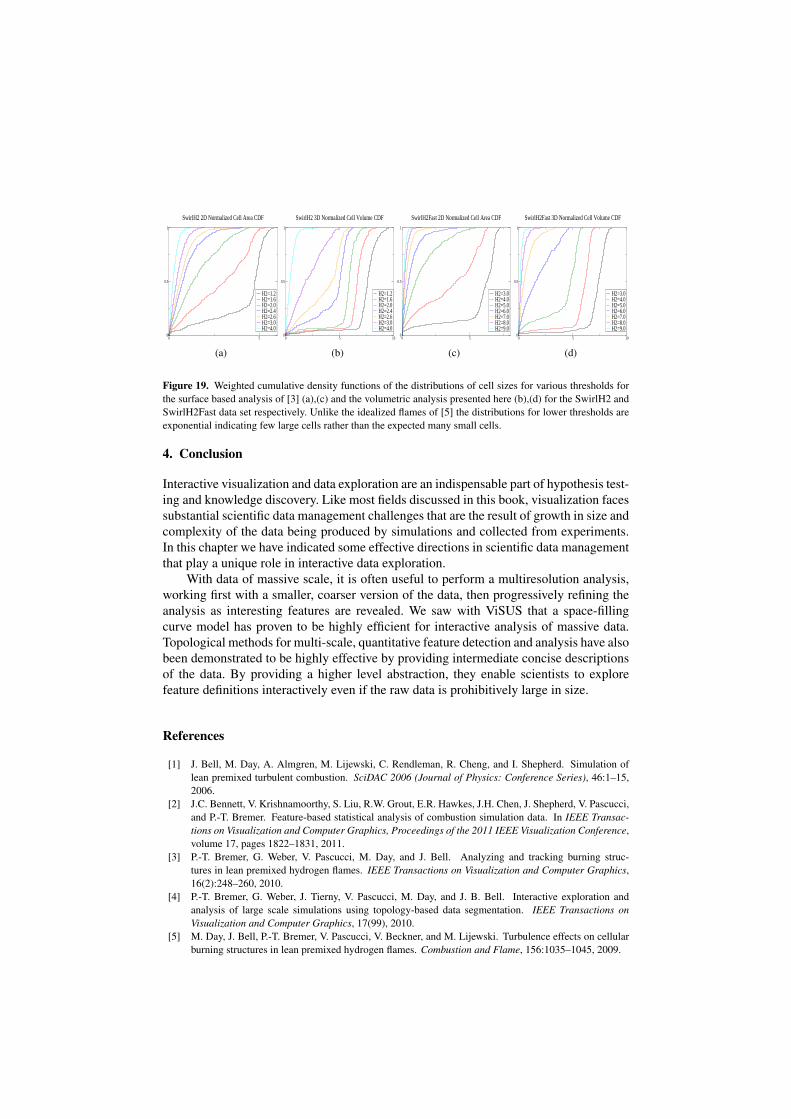
The hierarchical merge trees represent a meta-segmentation that can be explored inter-actively obtain reconstructions of the burning cells interactively. For example, Fig. 18shows the segmentation of the burning cells for two different thresholds of fuel con-sumption. The effective compression by only storing the meta-segmentation was abouttwo orders of magnitude. The ability to move between threshold parameters quickly al-lows parameter studies, such as illustrated in Fig. 19, where cumulative density functions(CDFs) of several statistics are shown for the burning cells. A traditional analysis of thisdata would require reprocessing the entire 8.4 terabytes of data 168 times, and instead,each new parameter study can be done in seconds.

0 50

0.5

1

H2=1.2H2=1.6H2=2.0H2=2.4H2=2.6H2=3.0H2=4.0

SwirlH2 2D Normalized Cell Area CDF

(a)

0 5 100

0.5

1

H2=1.2H2=1.6H2=2.0H2=2.4H2=2.6H2=3.0H2=4.0

SwirlH2 3D Normalized Cell Volume CDF

(b)

0 50

0.5

1

H2=3.0H2=4.0H2=5.0H2=6.0H2=7.0H2=8.0H2=9.0

SwirlH2Fast 2D Normalized Cell Area CDF

(c)

0 5 100

0.5

1

H2=3.0H2=4.0H2=5.0H2=6.0H2=7.0H2=8.0H2=9.0

SwirlH2Fast 3D Normalized Cell Volume CDF

(d)

Figure 19. Weighted cumulative density functions of the distributions of cell sizes for various thresholds forthe surface based analysis of [3] (a),(c) and the volumetric analysis presented here (b),(d) for the SwirlH2 andSwirlH2Fast data set respectively. Unlike the idealized flames of [5] the distributions for lower thresholds areexponential indicating few large cells rather than the expected many small cells.

4. Conclusion

Interactive visualization and data exploration are an indispensable part of hypothesis test-ing and knowledge discovery. Like most fields discussed in this book, visualization facessubstantial scientific data management challenges that are the result of growth in size andcomplexity of the data being produced by simulations and collected from experiments.In this chapter we have indicated some effective directions in scientific data managementthat play a unique role in interactive data exploration.

With data of massive scale, it is often useful to perform a multiresolution analysis,working first with a smaller, coarser version of the data, then progressively refining theanalysis as interesting features are revealed. We saw with ViSUS that a space-fillingcurve model has proven to be highly efficient for interactive analysis of massive data.Topological methods for multi-scale, quantitative feature detection and analysis have alsobeen demonstrated to be highly effective by providing intermediate concise descriptionsof the data. By providing a higher level abstraction, they enable scientists to explorefeature definitions interactively even if the raw data is prohibitively large in size.

References

[1] J. Bell, M. Day, A. Almgren, M. Lijewski, C. Rendleman, R. Cheng, and I. Shepherd. Simulation oflean premixed turbulent combustion. SciDAC 2006 (Journal of Physics: Conference Series), 46:1–15,2006.

[2] J.C. Bennett, V. Krishnamoorthy, S. Liu, R.W. Grout, E.R. Hawkes, J.H. Chen, J. Shepherd, V. Pascucci,and P.-T. Bremer. Feature-based statistical analysis of combustion simulation data. In IEEE Transac-tions on Visualization and Computer Graphics, Proceedings of the 2011 IEEE Visualization Conference,volume 17, pages 1822–1831, 2011.

[3] P.-T. Bremer, G. Weber, V. Pascucci, M. Day, and J. Bell. Analyzing and tracking burning struc-tures in lean premixed hydrogen flames. IEEE Transactions on Visualization and Computer Graphics,16(2):248–260, 2010.

[4] P.-T. Bremer, G. Weber, J. Tierny, V. Pascucci, M. Day, and J. B. Bell. Interactive exploration andanalysis of large scale simulations using topology-based data segmentation. IEEE Transactions onVisualization and Computer Graphics, 17(99), 2010.

[5] M. Day, J. Bell, P.-T. Bremer, V. Pascucci, V. Beckner, and M. Lijewski. Turbulence effects on cellularburning structures in lean premixed hydrogen flames. Combustion and Flame, 156:1035–1045, 2009.

[6] H. Edelsbrunner, J. Harer, and A. Zomorodian. Hierarchical Morse complexes for piecewise linear 2-manifolds. In Proceedings of the seventeenth annual symposium on Computational geometry, SCG ’01,pages 70–79, New York, NY, USA, 2001. ACM.

[7] A. Gyulassy, M. Duchaineau, V. Natarajan, V. Pascucci, E. Bringa, A. Higginbotham, and B. Hamann.Topologically Clean Distance Fields. IEEE Transactions on Visualization and Computer Graphics,13(6):1432–1439, November/December 2007.

[8] Rajkumar Kettimuthu and Others. Lessons learned from moving earth system grid data sets over a 20gbps wide-area network. In SC, pages 194–198. ACM, Proceedings of the 19th ACM InternationalSymposium on High Performance Distributed Computing (HPDC 2010).

[9] S. Kumar, V. Pascucci, V. Vishwanath, P. Carns, R. Latham, T. Peterka, M. Papka, and R. Ross. Towardsparallel access of multi-dimensional, multiresolution scientific data. In Proceedings of 2010 PetascaleData Storage Workshop, November 2010.

[10] S. Kumar, V. Vishwanath, P. Carns, B. Summa, G. Scorzelli, V. Pascucci, R. Ross, J. Chen, H. Kolla,and R. Grout. Pidx: Efficient parallel i/o for multi-resolution multi-dimensional scientific datasets. InProceedings of IEEE Cluster 2011, September 2011.

[11] Sidharth Kumar, Venkatram Vishwanath, Philip Carns, Joshua A. Levine, Robert Latham, GiorgioScorzelli, Hemanth Kolla, Ray Grout, Robert Ross, Michael E. Papka, Jacqueline Chen, and ValerioPascucci. Efficient data restructuring and aggregation for i/o acceleration in pidx. In Proceedings of theInternational Conference on High Performance Computing, Networking, Storage and Analysis, SC ’12,pages 50:1–50:11, Los Alamitos, CA, USA, 2012. IEEE Computer Society Press.

[12] J. K. Lawder and P. J. H. King. Using space-filling curves for multi-dimensional indexing. LectureNotes in Computer Science, 1832:20, 2000.

[13] A. Mascarenhas, R. W. Grout, P.-T. Bremer, E. R. Hawkes, V. Pascucci, and J.H. Chen. Topologicalfeature extraction for comparison of terascale combustion simulation data, pages 229–240. Mathematicsand Visualization. Springer, 2011.

[14] Y. Matsumoto. An Introduction to Morse Theory. Translated from Japanese by K. Hudson and M. Saito.American Mathematical Society, 2002.

[15] J. W. Milnor. Morse Theory. Princeton Univ. Press, New Jersey, USA, 1963.[16] V. Pascucci, D. E. Laney, R. J. Frank, G. Scorzelli, L. Linsen, B. Hamann, and F. Gygi. Real-time

monitoring of large scientific simulations. In Proceedings of the 2003 ACM symposium on Appliedcomputing, SAC ’03, pages 194–198, New York, NY, USA, 2003. ACM.

[17] Valerio Pascucci and Randall J. Frank. Global static indexing for real-time exploration of very large reg-ular grids. In Supercomputing ’01: Proceedings of the 2001 ACM/IEEE conference on Supercomputing(CDROM), pages 2–2, New York, NY, USA, 2001. ACM Press.

[18] Sujin Philip, Brian Summa, Peer-Timo Bremer, and Valerio Pascucci. Parallel Gradient Domain Pro-cessing of Massive Images. In Torsten Kuhlen, Renato Pajarola, and Kun Zhou, editors, EurographicsSymposium on Parallel Graphics and Visualization, pages 11–19, Llandudno, Wales, UK, 2011. Euro-graphics Association.

[19] Sujin Philip, Brian Summa, Valerio Pascucci, and Peer-Timo Bremer. Hybrid cpu-gpu solver for gradientdomain processing of massive images. In Parallel and Distributed Systems (ICPADS), 2011 IEEE 17thInternational Conference on, pages 244 –251, dec. 2011.

[20] Thierry Poinsot and Denis Veynante. Theoretical and Numerical Combustion. R.T. Edwards, secondedition, 2005.

[21] Alfredo Rodriguez, Douglas B. Ehlenberger, Patrick R. Hof, and Susan L. Wearne. Three-dimensionalneuron tracing by voxel scooping. Journal of Neuroscience Methods, 184(1):169 – 175, 2009.

[22] Hans Sagan. Space-Filling Curves. Springer-Verlag, New York, NY, 1994.[23] B. Summa, G. Scorzelli, M. Jiang, P.-T. Bremer, and V. Pascucci. Interactive editing of massive imagery

made simple: turning Atlanta into Atlantis. ACM Trans. Graph., 30:7:1–7:13, April 2011.[24] J. S. Vitter. External memory algorithms and data structures: Dealing with massive data. ACM Comput-

ing Surveys, March 2000.[25] Forman A. Williams. Combustion Theory. Westview Press, second edition, 1994.