scalable validation of data streams - uppsala university · scalable validation of data streams ......
TRANSCRIPT
ACTAUNIVERSITATIS
UPSALIENSISUPPSALA
2016
Digital Comprehensive Summaries of Uppsala Dissertationsfrom the Faculty of Science and Technology 1384
Scalable Validation of Data Streams
CHENG XU
ISSN 1651-6214ISBN 978-91-554-9600-5urn:nbn:se:uu:diva-291530

Dissertation presented at Uppsala University to be publicly examined in room 2446, ITCbuilding 2, Lägerhyddsvägen 1, Uppsala, Wednesday, 17 August 2016 at 13:15 for the degreeof Doctor of Philosophy. The examination will be conducted in English. Faculty examiner:Professor Byung-Suk Lee (University of Vermont).
AbstractXu, C. 2016. Scalable Validation of Data Streams. Digital Comprehensive Summaries ofUppsala Dissertations from the Faculty of Science and Technology 1384. 51 pp. Uppsala:Acta Universitatis Upsaliensis. ISBN 978-91-554-9600-5.
In manufacturing industries, sensors are often installed on industrial equipment generating highvolumes of data in real-time. For shortening the machine downtime and reducing maintenancecosts, it is critical to analyze efficiently this kind of streams in order to detect abnormal behaviorof equipment.
For validating data streams to detect anomalies, a data stream management system calledSVALI is developed. Based on requirements by the application domain, different stream windowsemantics are explored and an extensible set of window forming functions are implemented,where dynamic registration of window aggregations allow incremental evaluation of aggregatefunctions over windows.
To facilitate stream validation on a high level, the system provides two second ordersystem validation functions, model-and-validate and learn-and-validate. Model-and-validateallows the user to define mathematical models based on physical properties of the monitoredequipment, while learn-and-validate builds statistical models by sampling the stream in real-time as it flows.
To validate geographically distributed equipment with short response time, SVALI is adistributed system where many SVALI instances can be started and run in parallel on-boardthe equipment. Central analyses are made at a monitoring center where streams of detectedanomalies are combined and analyzed on a cluster computer.
SVALI is an extensible system where functions can be implemented using external librarieswritten in C, Java, and Python without any modifications of the original code.
The system and the developed functionality have been applied on several applications, bothindustrial and for sports analytics.
Keywords: Data Stream Management, Distributed Data Stream Processing, Data StreamValidation, Anomaly Detection
Cheng Xu, Department of Information Technology, Division of Computing Science, Box 337,Uppsala University, SE-75105 Uppsala, Sweden.
© Cheng Xu 2016
ISSN 1651-6214ISBN 978-91-554-9600-5urn:nbn:se:uu:diva-291530 (http://urn.kb.se/resolve?urn=urn:nbn:se:uu:diva-291530)
To my parents and grandparents 致青春

List of Papers
This thesis is based on the following papers, which are referred to in the text by their Roman numerals.
I C. Xu, E. Källström, T. Risch, J. Lindström, L. Håkansson, and J. Larsson: Scalable Validation of Industrial Equipment using a Functional DSMS, submitted for journal publication, 2016. I am the primary author of this paper.
II S. Badiozamany, L. Melander, T. Truong, C. Xu, and T. Risch: Grand Challenge: Implementation by Frequently Emitting Parallel Windows and User-Defined Aggregate Functions, Proc. The 7th ACM International Con-ference on Distributed Event-Based Systems, DEBS 2013, Arlington, Texas, USA, June 29 - July 3, 2013. I contributed 50% of the implementation work and 30% of the writing. Au-thors are listed in alphabetic order.
III C. Xu, D. Wedlund, M. Helgoson, and T. Risch: Model-based Validation of Streaming Data, The 7th ACM International Conference on Distributed Event-Based Systems, DEBS 2013, Arlington, Texas, USA, June 29 - July 3, 2013. I am the primary author of this paper.
Reprints of the papers were made with permission from the publishers. All papers are reformatted to the one-column format of this book.

Other Publications
IV M. Leva, M. Mecella, A. Russo, T. Catarci, S. Bergamaschi, A. Malagoli, T. Risch, C. Xu and L. Melander: Visually Querying and Accessing Data Streams in Industrial Engineering Applications, 21st Italian Symposium on Advanced Database Systems, SEBD 2013, Roccella Jonica, Italy, June 30th - July 3rd, 2013.
V E. Källström, C. Xu, T. Risch, J. Lindström, L. Håkansson, and J. Larsson: Anomaly detection over streaming data, submitted for journal publication, 2016.

Contents
1 Introduction ......................................................................................... 11 2 Background and related Work ............................................................. 13
2.1 Data Stream Management Systems ................................................. 13 2.1.1 Data Stream Elements ............................................................ 13 2.1.2 Continuous Queries ................................................................ 14
2.2 Stream Windows ............................................................................. 15 2.3 Window Operators .......................................................................... 17 2.4 Distributed DSMSs ......................................................................... 18 2.5 Stream Anomaly Detection ............................................................. 19 2.6 AMOS II and SCSQ ........................................................................ 19
3 The SVALI (Stream VALIdator) System ............................................ 21 3.1 System Architecture ........................................................................ 22
3.1.1 Data source systems ............................................................... 25 3.2 The Equipment Model .................................................................... 26 3.3 Stream windows .............................................................................. 28
3.3.1 Window forming functions .................................................... 29 3.3.2 Window Operators ................................................................. 30 3.3.3 User Defined Incremental Window Aggregation .................. 31 3.3.4 Implementation ...................................................................... 32
3.4 Data Stream Validation ................................................................... 35 3.4.1 Model-and-validate ................................................................ 36 3.4.2 Learn-and-validate ................................................................. 36
4 Technical Contributions ....................................................................... 38 4.1 Paper I ............................................................................................. 38 4.2 Paper II ............................................................................................ 39 4.3 Paper III .......................................................................................... 40
5 Conclusions and Future Work ............................................................. 41 6 Summary in Swedish ........................................................................... 43 7 Acknowledgements.............................................................................. 45 Bibliography ................................................................................................. 47

Abbreviations
DBMS Database Management System DSMS Data Stream Management System SQL CQ
Structured Query Language Continuous Query


11
1 Introduction
Traditional database management systems (DBMSs) store data records per-sistently while queries over the current state of the database contents are executed on demand. This fits well for business applications such as bank and accounting systems. However, in the last decades, more and more data are generated in real-time, e.g. data from stock markets, real time traffic, click-streams on the internet, sensors installed in the machines, etc. Such data continuously generated in real time is called data streams. The rate at which data streams are produced is often very high e.g. megabytes per sec-ond, which makes it infeasible to first store streaming data on disk and then query it. Furthermore, business decisions and production systems rely on short response times so the delay caused by first storing the data in a data-base before querying and analyzing it may be unacceptable. For example, monitoring the healthiness of different components in industrial equipment requires the system to return the result within seconds. Data stream man-agement systems (DSMSs), such as AURORA [2], STREAM [8], and SCSQ [69], are designed to deal with this kind of applications. Instead of ad-hoc queries over static tables, queries over streams are continuous queries (CQs) since they are continuously running until they are explicitly terminated and will produce a result streams as long as they are active. Furthermore, since data streams often are extremely large or infinite, the processing is often made over only the most recent stream elements, called a stream window.
In order to deliver quality services for industrial equipment it can be con-tinuously monitored to detect and predict failures. As the complexity of the equipment increases, more and more research is conducted to automatically and remotely detect abnormal behavior of machines [55]. For example, Volvo Construction Equipment (Volvo CE) has installed a component called automatic transmission clutches to monitor the health of the clutch material of their L90F wheel loaders. Various sensors measuring different signal variables are installed on the wheel loaders and data from the sensors are delivered following the CANBUS protocol [21], which is an industry stan-dard protocol to communicate with the data buses in engines and other ma-chines. Expensive statistical computations over the data are required in real-time to detect and predict anomalies so that corresponding actions can be taken to reduce the cost of maintenance. Furthermore, when the number of monitored machines increases it is also important that the processing scales.

12
In order to validate that the equipment functions according to its specifi-cation, streaming data needs to be analyzed in real-time. With our approach, validation of equipment then becomes a special kind of CQs that analyze streams from equipment sensors in terms of mathematical models and data stored in a local database inside the DSMS. This defines the research ques-tions of this Thesis:
1. The overall research question is: How should a data stream man-agement system be designed to enable scalable validation of cor-rect behavior of distributed industrial equipment?
2. What types of stream windows should be defined in order to sup-port analyzes of measurement streams from industrial equipment?
3. How should mechanisms for validating correct behavior of moni-tored equipment on a high and user-oriented level using CQs be defined?
4. How can scalable and efficient stream validation be imple-mented?
In order to answer research question one above, a system called SVALI (Stream VALIdator) was developed and evaluated in real industrial applica-tions. Paper I describes the overall architecture of SVALI and shows how it has been used for detecting abnormal behavior of industrial equipment in use.
Paper II presents SVALI’s window operators suitable for real-time analy-sis of data from real soccer matches. In particular, the FEW windows were proposed and evaluated that emits result early, before complete windows are formed. Furthermore, generalized user defined stream aggregation functions allowed incremental maintenance of both statistics and dictionaries. More new window types are proposed in Paper I and Paper III, leading to an ex-tensible window mechanism in SVALI where users can add new kinds of windows as described in Chapter 3. This answers research question two.
SVALI provides second order system validation functions model--and-validate and learn-and-validate to specify on a high level CQs calling vali-dation models as parameters, as shown in Paper I and Paper III. The models are expressed as formulae over streamed data values. For applications where no physical model can be easily defined, the system can also dynamically learn a model. This answers research question three.
Window forming functions with user defined aggregations in SVALI are evaluated in Paper II while parallel execution of validation functions is evaluated in Paper I and Paper III. This answers research question four.
The Thesis is organized as follows. In Chapter 2, related technologies are introduced along with references to the contribution of the thesis. Chapter 3 presents the overall architecture of SVALI and its implementation. Chapter 4 summarizes the technical contributions of the research papers on which the Thesis is based. Finally, conclusions and future work are discussed in Chap-ter 5.
13
2 Background and Related work
This chapter describes the background of this thesis work. It includes fun-damental technologies for Data Stream Management Systems, Data Stream Windows, Window Operators, Distributed Databases, and Stream Anomaly Detection. It furthermore introduces the AMOS II and SCSQ systems, which SVALI extends.
2.1 Data Stream Management Systems While DBMSs are designed to manage persistently stored data, DSMSs are developed to deal with applications where data is generated continuously in real-time, such as scientific instruments, industrial manufacturing, stock marketing, and traffic monitoring. In the past decades, several DSMS re-search prototypes were proposed and implemented such as Aurora [1][2][24][28], STREAM [8][10], NiagaraCQ [27][43][44][46], Gigascope [30], TelegraphCQ [26][42][52][66], XStream [36][37], and SCSQ [69]. Some of the prototypes have further been developed as commercial DSMSs. For example, Aurora is the predecessor of StreamBase [60].
2.1.1 Data Stream Elements
A data stream [2][8][11][51][66] is a sequence of continuously delivered data stream elements each containing one or several measurements or events. Stream elements have the format:
(ts, v1, v2, … , vi) Each stream element contains a set of attributes a1, a2, … , ai with values v1, v2, … , vi . Stream elements can either have uniform or variable number of attributes.
A time stamp attribute, ts, can be attached to stream elements. The mean-ing of a time stamp varies. It can, for example, represent:
1. The time when the values were measured [2].
2. The time when the stream elements arrived into the DSMS [8][66].

14
Some DSMSs consider time stamp as a special attribute which is not part of the schema [2][8], while others [2][51] provide both a tuple identifier (ID) and a time stamp as special attributes.
The semantics of data streams are also discussed in terms of reconstitu-tion functions [46] to represent formally data streams of various forms, for example, streams of measurements indicating changes of the measured at-tributes over time. Another approach is tagged streams [35] where stream elements are represented as insert, update, or delete operations.
Stream tuples may also have a valid time interval as two time stamp at-tributes, start time and end time [30] representing the time during which an event happened.
In SVALI the time stamp is normally represented as a real number denot-ing the number of seconds from a system wide epoc, currently Jan 1, 1970. Both implicit and explicit time stamps are supported in SVALI.
2.1.2 Continuous Queries
One major difference between traditional DBMSs and DSMSs is that the size of a data stream is potentially unbounded and it is not feasible to know the complete state of it when it is queried, so regular passive queries are not sufficient for searching data streams. Data delivered as streams requires con-tinuous queries (CQs) [2][6][11][51][66], which are queries over streams that continuously deliver new results as new data arrives to the stream. For example, if some machines continuously deliver streams of temperature readings, a continuous query may be:
“Continuously show me the temperature readings for sensor X on equip-ment of model Y when it is 20% higher temperature than what is specified.”
CQs registered for a stream are applied either over each most recent stream element as the above example or over a set of recent stream elements, a stream window, to continuously deliver results to the end-users. An exam-ple of a CQ applied on a stream window is:
“Continuously show me the average temperature readings for sensor X on equipment of model Y every 10 minutes when the average temperature is 20% higher than what is specified.”
In SVALI, CQs are defined as parameterized functions that continuously iterate through stream elements and emit streams of results [39]. Arbitrary functions can be applied on the stream elements to do numerical computa-tions and filter data.
In Aurora [2], CQs are defined graphically using a boxes and arrows paradigm, where tuples flow through a loop free graph of processing opera-tors. Basic operators include Window, Filter, Drop, Map, Group-By, and Join. Paper IV describes a graphical CQ formulation system for SVALI. STREAM [8] extends the relational database model in order to cope with data streams where windows are considered as periodically updated rela-
15
tions. The query language of STREAM is called CQL [10]. In the STREAM model, relations to relations are regular SQL queries; Streams to relations are queries over windows; Relations to streams return three kinds of streams: Istream (insert stream), Dstream (deletion stream), and Rstream (relation stream).
Some of the DSMS systems are designed for special applications. For ex-ample, NiagaraCQ [27][48] was initially designed for efficient search of XML files over the internet by exploring shared computations between CQs. The extension for XQuery to support data streams and window functions in [19] was designed for XML streams. Gigascope [30] was developed for net-work applications to analyze the status of the networks and detect intrusions. XStream [36][37] was designed for analyzing data streams and provides a library of signal processing functions such as FFT. For domain-specific stream processing, SVALI provides foreign functions that utilize external libraries for different applications.
All DSMSs discussed so far, including SVALI, provide high-level de-clarative user specifications of data stream filters, joins, and transformations based on CQs. There are also libraries and web services for data stream pro-gramming such as Storm [7], Spark Streaming [58], Flink Streaming [6], and Amazon Kinesis [4] that can be used to develop distributed stream process-ing programs. By contrast, this thesis work is based on a high-level, user-oriented, and declarative data stream query language.
2.2 Stream Windows A window is a bounded recent set of stream elements over an infinite stream [2][8][11][18][19][38][50][51][66]. It reflects the current state of a stream and changes as new data elements arrives from a stream.
The window extent is the set of stream elements in a window. The win-dow extent can be formed in different ways. For example, with count-based windows the extent has a fixed number of stream elements, with time-based windows the extent is defined by a time span of time stamped stream ele-ments, while the extent of a landmark window contains a growing set of all stream elements from some starting point.
The window progress defines how the window moves forward. When it progresses an old window instance is emitted and a new one starts to be formed. For example, the window might progress every 10 stream elements or every 10 seconds.
When the window progresses and a complete window is formed and emit-ted, a window time stamp can be assigned to the emitted window. There are different options for defining the time stamp of a window, e.g. (i) the time stamp of the first element in the window, (ii) the time stamp of the last ele-ment in the window, or (iii) the system time when the window is emitted. In

16
SVALI, a stream window is regarded as a stream element having the time stamp when it was emitted.
The window size, sz, is the number of stream elements in a window ex-tent. For count-based windows the size sz is defined by the number of ele-ments in the window, while for time-based windows, it is defined by time span between the first and the last stream elements.
The window stride, st, is the number of stream elements that expire from a window as the window progresses. For example, for sliding windows the stride st is less than the size sz, while for tumbling window sz = st. For time windows, the stride is defined as the time span between when it was formed and when it progresses.
Figure 1 illustrates simple examples of count based tumbling and sliding windows.
Figure 1 (a) count (sliding) window with the size sz = 5, stride st = 2
Figure 1 (b) count (tumbling) window with the size sz = 5, stride st = 5
SVALI provides an extensible mechanism for defining different kinds of window semantics [2][8][18][19][38][51]. The following basic window kinds are supported by SVALI:
• Sliding count windows are windows where the number of elements in the window is constantly sz and which progresses with a constant number of elements st < sz elements. For example, sliding count windows can be used for calculating statistics of sensor readings with a fixed polling frequency.
• Sliding time windows are windows where the elements in the win-dow are those measurements arriving during a constant time span sz which progresses every st < sz time units. For example, in Paper II, one minute sliding time windows with one sec stride are used for analyzing running statistics of players in a soccer match.
17
• Tumbling count windows are windows where the number of ele-ments in a window is constantly sz and which progresses when the window is full, i.e. sz = st elements. As sliding count windows, tum-bling count windows can be used to calculate statistics over streams with fixed rates.
• Tumbling time windows are windows where the elements are those arriving during a constant time span sz and which progresses when the time span is expired, i.e. sz = st time units. Similar to sliding time windows, tumbling time windows are usually used for comput-ing running statistics over time stamped streams. For example, in the linear road benchmark [9] one minute tumbling time windows are created to collect road traffic statistics.
2.3 Window Operators As a window can be seen as a temporary database relation in memory, basic relational operators also apply on windows. Commonly used operators are: windows to relations, window selections, window projections, and window aggregations [8][10].
Windows to Relations. Regular database relations are represented as bags, which do not guarantee element orders. Therefore, in order to preserve the order property of a window, in SVALI the vector data type is used to represent the sequence of elements in a window.
Window Projection and Selection. Window projection and selection over a window w can be expressed as: Π a1, a2, … , an (w) where σφ(w) where a1, a2, … , an are attributes of w and φ is a predicate over the extent
of w. Note that when the time stamp attribute ts is included in the stream tuples
either implicitly or explicitly, window projection and selection also contains the ts as one of the attributes in the result.
Window Aggregations are aggregate function over window extents. A naïve implementation of window aggregations first materializes the extent and then computes the value of the aggregate function, which has the disad-vantage of being space consuming and inefficient for sliding windows with small strides [17]. SVALI supports dynamic and incremental computation of window aggregations without need for materialization of the window extent. This mechanism furthermore generalizes conventional aggregation by allow-ing incrementally maintaining any data structure as windows progresses, for example the heat map table of statistics in Paper II.

18
2.4 Distributed DSMSs Some DSMS prototypes [2][8] were initially developed as centralized sys-tems where all the data streams are sent to the system for analysis. This may have some scalabilities problems. For example, when the stream data vol-ume is scaled up, how can the system still keep up with the real-time re-quirements? When the number of data stream sources is scaled up, how can the DSMS process all the data streams while still keeping up?
The first direction in improving scalability is to analyze the query execu-tion plan and place different operators in an optimized order [13][14][59][71]. Load sharing between different operators is often done by pushing up or pushing down operators depending on selectivity and cost estimates. A second direction is to implement special algorithms over sliding windows, where the aggregated results can be calculated incrementally [12][31][43]. A third direction is to have load shedding strategies to return approximated results [3][15][57][62][63].
In particular, to ease the scalabilities issues of a centralized DSMS, dis-tributed DSMSs [28][49][59][69][71] were developed that can efficiently process CQs over high volume data streams in parallel. For example, high volume streams are split and then expensive queries over each sub stream are executed in parallel, over which the results are aggregated [28][69].
SVALI utilizes the parallelization strategies of SCSQ [69]. In SVALI, DSMS engines are installed both on-board the monitored equipment and in a central parallel monitoring cluster to which streams are emitted from the on-board SVALI engines using stream uploaders. The monitoring server can be accessed via a client server API to change the parameters of CQs while they are running.
For network applications in a distributed setting, to save transmission and communication costs it is desirable to place some of the operators as close to the source site as possible [49][59]. Therefore operator placements in the network are an optimization problem for data stream processing, where both a greedy (sub-optimal) and optimal algorithms can be used [59]. In SVALI, this is handled by executing CQs in SVALI systems running on-board moni-tored equipment. Local CQs making complex computations rather than just simple filters can be run on-board to reduce the data stream volumes [49].
Aurora* [28] proposed an approach for a distributed environment where different participating nodes from different domains are cooperating. It en-ables intra-participant distribution where a name server has full control of all the Aurora servers. Any operators or sub-queries can be placed in any of the Aurora nodes within the application domain. Medusa [28] allows inter-participant distribution, in which several autonomous participants are col-laborated. In SVALI, a meta-data schema describes all kinds of monitored equipment in use. A name server keeps track of all distributed SVALI peers.

19
2.5 Stream Anomaly Detection The task of stream anomaly detection is to analyze the status of data streams to detect measurements that significantly deviate from expected values [5][23][40][41][54][67][70]. This can be considered as a data stream mining problem to continuously detect outliers in streams [33][61][68]. This is dif-ferent from regular data mining, which is done in a store and process fash-ion. Three main approaches have been proposed for detecting outliers in the data streams, i) distance-based outlier detection [5][33][41][61][67] and Paper V. ii) density-based outlier detection [61][67]. iii) angle-based outlier detection [68]. Distance-based outliers are specified by two parameters, k and d. A stream element is an outlier when there are no more than k elements within d distance from it. Density-based outliers are defined similar as den-sity based cluster algorithm, where a stream element is an outlier when it is neither a core point nor an edge point [67]. Angle-based outliers are done by ranking the value of angle-based outlier factor [68]. A stream element is defined as an outlier when it is ranked in the least-k list.
Historical data are often very useful for building real-time outlier detec-tion models [40][70], especially when online data streams are dynamically changing or containing random noise. By utilizing historical data, the online detecting algorithm can be refined and smoothed [40]. This often can be done in two phases: offline learning, and online learning [70]. SVALI pro-vide two system functions, model_n_validate() and learn_n_validate() to monitor data streams from equipment. The model can be either built offline, as in Paper I, or online, as in Paper III, and then stored in the main memory database for online validations.
2.6 AMOS II and SCSQ This thesis work is built on top of the functional database management sys-tem AMOS II [39] and the DSMS SCSQ [69]. The basic primitives of the AMOS II functional data model are objects, types, and functions. AMOS II has two kinds of objects, literal and surrogate objects, where literals are im-mutable objects like numbers and strings while surrogate objects are mutable based OIDs managed by the system. Objects can also be collections. A query in AMOS II is defined through a select statement where a variable can be bound to typed objects from any domain, and functions can be used in both the result and the condition. Stored functions model the attributes of entities and relationships between them. Derived functions define views as queries over other functions. They are similar to views in relational DBMS, but can be parameterized views similar to prepared queries in JDBC. Foreign func-tions are (parameterized) functions defined in external programming lan-guages such as C or Java.
20
SCSQ [69] is a Data Stream Management system that enables queries over large volume data streams by massive parallelization. It enables high level specifications of distributed stream queries with advanced computa-tions. The scalability problem is alleviated by splitting streams into sub-streams, over which expensive CQs can be executed in parallel. The stream query language called SCSQL allows the user to specify the parallelization strategies on a high level.
The SVALI system extends both AMOS II and SCSQ. Detailed descrip-tions about the contributions of this thesis are presented in the next chapter.
21
3 The SVALI (Stream VALIdator) System
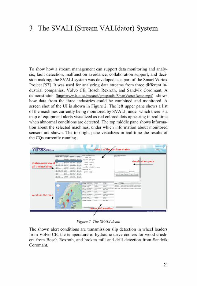
To show how a stream management can support data monitoring and analy-sis, fault detection, malfunction avoidance, collaboration support, and deci-sion making, the SVALI system was developed as a part of the Smart Vortex Project [57]. It was used for analyzing data streams from three different in-dustrial companies, Volvo CE, Bosch Rexroth, and Sandvik Coromant. A demonstrator (http://www.it.uu.se/research/group/udbl/SmartVortexDemo.mp4) shows how data from the three industries could be combined and monitored. A screen shot of the UI is shown in Figure 2. The left upper pane shows a list of the machines currently being monitored by SVALI, under which there is a map of equipment alerts visualized as red colored dots appearing in real time when abnormal conditions are detected. The top middle pane shows informa-tion about the selected machines, under which information about monitored sensors are shown. The top right pane visualizes in real-time the results of the CQs currently running.
Figure 2. The SVALI demo
The shown alert conditions are transmission slip detection in wheel loaders from Volvo CE, the temperature of hydraulic drive coolers for wood crush-ers from Bosch Rexroth, and broken mill and drill detection from Sandvik Coromant.

22
The rest of this chapter presents the architecture of SVALI and highlights my contributions to it.
3.1 System Architecture Figure 3 illustrates the architecture of the Stream VALIdator (SVALI) sys-tem.
Figure 3. SVALI architecture
The SVALI architecture consists of three software layers: applications, monitoring server, and data source systems.
In the figure data streams from different data sources are emitted to a SVALI monitoring server at a monitoring site. The monitoring server proc-esses queries that transform, combine, and analyze data streams from differ-ent streaming data sources. Different kinds of application programs access the monitoring server to perform various analyses. The applications access the monitoring center by sending CQs to it through the external API. The application can be, e.g., a visualizer that graphically displays data streams derived from malfunctioning equipment to indicate what is wrong, a graphi-

23
cal query formulator, Paper IV, with which CQs are constructed on a high level, or a stream logger that saves derived streams on disk as CSV files.
SVALI is a distributed DSMS so that SVALI peers can be installed not only in the monitoring site but also directly on-board the monitored equip-ment or as clients to other SVALI peers. Each SVALI peer manages its own main-memory database that contains an ontology and local data.
As shown in the figure, a global ontology, describing meta-data about all kinds of monitored equipment, is installed in the monitoring server, while local ontologies, describing particular monitored equipment, are installed in SVALI peers running at different source sites.
The global ontology integrates data from different streaming data sources. It is organized in three levels. The validation model, presented in Section 3.4, identifies anomalies in monitored equipment in terms of the equipment model. The equipment model is a common meta-data model that describes general properties common to all kinds of equipment, e.g. meta-data about sensor models and wheel loaders. The equipment model for our scenario application is shown in Figure 5. The data source model maps raw data from different data sources to the equipment model.
The local ontology on a site also has three levels. The local data source model maps raw data for a particular kind of data source to the equipment model. In order to identify anomalies locally for each monitored machine, a local validation model is installed at each site. Since each streaming data source is encapsulated by a SVALI peer, local CQs can be executed over the local ontology. This enables each peer to analyze local data streams to pro-duce reduced streams of anomaly measurements, which are continuously emitted to the monitoring server where anomalies from many sites are col-lected, combined, and analyzed. In Paper I it is shown how local validation enables efficient and scalable monitoring of the expected behavior of each wheel loader.
To handle computations in CQs that cannot be expressed as built-in func-tions and operators, the SVALI engine provides a plug-in mechanism where algorithms defined in various programming languages can be called in CQs. Examples of algorithms are numerical computations, pattern matchings, optimizations, and classifications. Plug-ins for Python and Java engines are available so that algorithms written in these languages can be used by SVALI without any changes of the original code.
SVALI can hook up to new kinds of equipment by defining data stream interfaces to SVALI systems running on-board the monitored equipment via the plug-in mechanisms. Once a data stream interface is defined for a par-ticular kind of streaming data source the data streaming from any instances of an interfaced source can be freely used in CQs processed by SVALI. The derived data streams produced by local CQs can be forwarded to other SVALI nodes or to applications.

24
Figure 4 summarizes the implemented contributions of this Thesis.
Figure 4. implemented contributions of SVALI
The SVALI system is built on top of the SCSQ data stream management system.
1. Data Stream Interfaces define stream interface functions that map external raw data streams into the internal format that SVALI sup-ports. For example, in Paper III, raw data streams are streamed from a CORENET server to SVALI through the CORENET data stream interface. In Paper I, we developed a data stream interface called the CANBUS data stream interface that follows the standard CANBUS protocol.
2. Window forming functions are SVALI functions that construct new windows of different kinds and then maintain the data structures to represent the states of the windows as they progress. The internal functioning of window forming functions will be described in Sec-tion 3.3.1.
3. The stream uploader, described in Paper I, continuously transmits data streams to the monitoring server. Security is increased by hav-ing a firewall between monitoring servers and the data sources.
4. The three level ontology is the meta-data for monitored equipment described above. The data source model semantically enriches the raw data streams. The equipment model describes the meta-data about all kinds of machines in different application scenarios. The validation model utilizes the stream validator and the equipment model to validate data streams of different kinds defined by data source models.
SCSQ
Data Stream Interfaces
plug-in to external libraries
DSMS client server API
stream validator
model and validate
learn and validateequipment model
data source model
validation model
ontology
input stream
input stream
input stream
stream uploader
window forming functions
25
5. The stream validator implements the two ways of validating data streams: model-and-validate and learn-and-validate as described in Paper I and Paper III. Instead of writing complex CQs the user only needs to define a model function and a validate function which are passed to either model_n_validate() or learn_n_validate(). As shown in Paper I and Paper III, when pushing down the validation func-tions as close as possible to the data stream sources the stream vol-umes can be significantly reduced and thus reduces the communica-tion costs between data sources and the monitoring server.
6. Plug-ins to external libraries allows to import external data mining algorithms as foreign functions to be used in CQs. For example, in Paper I, the validation function uses statistical algorithms that are implemented in Python.
3.1.1 Data source systems
Raw data streams are generated at different sites. Examples of producers of raw data streams are: sensors installed in the hardware equipment, transac-tion logs, and other data stream producing software. The data stream inter-faces transform the raw data into the internal format supported by SVALI.
Rather than having to define new data stream interfaces for every kind of data stream source, the data stream interfaces are implemented as parameter-ized functions that support a communication protocol for communication with a particular kind of streaming data source. For example, if several dif-ferent machines deliver streaming data using the same protocol, the same generic data stream interface function can be used for all instances of the same equipment, where function parameters specify the identity and other properties of each accessed data stream.
In Figure 3, one source is data streams from wheel loaders at Volvo CE, which are streamed to the monitoring server through a SVALI peer via a CANBUS data stream interface. A second stream data source is the stream from a milling machine at Sandvik Coromant through the CORENET data stream interface. Another important kind of data source is CSV files contain-ing logged data streams. A CSV reader reads CSV files and emits the rows as data stream elements to SVALI.
The data format produced by a data stream interface is represented on a low level as raw data tuples, which are numerical vectors contain no meta-data about the values in the fields of a stream element, making the CQs very unintuitive and error prone. To enable defining CQs over data streaming from monitored equipment in terms of the equipment model the raw data streams need to be semantically enriched by mapping the raw data tuples to the equipment model. This makes CQs meaningful and easier to understand than CQs directly over raw data streams.
26
Consider a very simple example of a CQ to return a derived stream of time stamped power consumption measurements exceeding 10 KW from a raw data stream of vectors s. Without any semantic enrichment, the CQ is formulated as: select e[0], e[4]
from Stream s, Vector of Number e
where millRow[4] > 10 and e in s;
Here, the in operator extracts elements e from the stream s. The semanti-cally enriched CQ is formulated as: select timeStamp(e), power(e)
from Stream s, Vector of Number e
where power(s) > 10 and e in s;
In this case, the data source model uses two derived functions defined over the raw stream tuple e: create function timeStamp(Vector e) -> Number as e[0];
create function power(Vector e) -> Number as e[4];
Another advantage of the semantic enrichment is that one can overload the access functions so that the data formats in the streams can evolve with-out changing any CQs that use the meta-data functions. For instance, if the format of the stream tuple is changed from vectors to JSON records, one only needs to redefine the access functions: create function timeStamp(Record e) -> Number as e[“ts”];
create function power(Record e) -> Number as e[“power”];
One problem with semantic enrichment is that when there are many dif-ferent kinds of streams one needs to manually define an access function for each attribute in the stream tuples. When the number of attributes is large, the definition of access functions becomes tedious.
To simplify the task of defining access functions for streams, SVALI pro-vides a mechanism to generate access functions based on meta-data in the data source model. Instead of defining the functions accessing stream ele-ment attributes manually, semantics about the stream elements are stored as meta-data and used to automatically generate the access functions.
3.2 The Equipment Model Figure 5 shows SVALI’s equipment model for Smart Vortex [57]. It con-tains the ontology for the applications.

27
Figure 5. Meta-data Schema
A hierarchy of stream objects is presented at the top. The type DataStream is a super-class representing all kinds of data streams. RawDataStream and StoredStream are its subclasses. RawDataStream represent streams that are generated directly from equipment. In Sandvik Coromant, the data is gener-ated from sensors installed on machines transmitted by CORENET, this is modeled as CORENETStream being a subclass of RawDataStream. The data from wheel loaders at Volvo CE are streamed following the CANBUS pro-tocol. This is modeled as CANBUSStream, which is also a subclass of Raw-DataStream. Similarly, HagglundsStream represents the stream from Bosch Rexroth. There might also be more specific stream subclasses, for example in Sandvik, MillStream and DrillStream are streams from mill machines and drill machines, respectively.
At the bottom of the figure, the type Machine represents different models of machines. MachineInstallation represents a physical machine located at a Location. The type Sensor describes the properties of different kinds of sen-

28
sor models. There is a set of SensorInstallations on each machine installa-tion. A SensorInstallation generates a RawDataStream.
3.3 Stream windows In order to facilitate the advanced monitoring required by our applications, SVALI provides an extensible set of stream window semantics in addition to the basic window primitives described in Section 2.2. The following kinds of windows are in particular needed by the applications:
• Partition windows are tumbling windows where new windows are started when a certain stream element attribute changes. Time or count windows cannot be used to identify this kind of windows be-cause the window size is dynamically varying. For example, the window progresses when an attribute ag indicates the current gear of a wheel loader and its value vg changes between two consecutive stream elements. Notice that this is different from the partition win-dows in [38][48], because in SVALI new partition windows are cre-ated whenever a partitioning attribute changes between consecutive stream elements (Paper I), rather than splitting the stream based on some attribute(s).
• Predicate windows are windows where the start and stop points of a window are defined as predicates that determine the extent of the window. As partition windows, the window size is varying and de-pends on two predicates. For example, in Sandvik the matching process cycle is indicated by a flag, so the window starts when the flag is changed from 0 to 1 and stops when the flag is changed from 1 to 0. Another example is forming windows when some attribute, e.g. temperature, of consecutive stream elements are larger than a threshold, e.g. 100 ºC. The window starts to accumulate stream ele-ments when the temperature is larger than 100 ºC and the window is emitted when the temperature becomes lower than 100 ºC. Unlike the predicate window in [34] being a condition over the latest state of an object property, in SVALI predicate windows are defined as state changes over successive stream element attribute values.
• Frequently emitted windows. Another issue is how often results are emitted from windows, the window emitting rate r. Statistics over window extents are usually emitted when the window pro-gresses. This causes delays for large window sizes. For example, in Paper II, 10 minutes time windows over soccer match data is formed. However, the partially aggregated data needs to be emitted every minute, rather than waiting 10 minutes for the full aggregation to be emitted. To reduce the delay of the emitted results they can be
29
delivered before the window progresses. This is supported in SVALI by a special kind of window called frequently emitted windows (FEW) where the emission rate can be specified as a parameter. For example, for a time window of size sz = 10 minutes, the emitting rate may be one minute, so that statistics are delivered every minute without waiting for the complete 10 minutes window to be formed.
3.3.1 Window forming functions
Different kinds of streams of windows are formed by corresponding window forming functions. They are SVALI functions that construct, maintain, and emit stream windows of a specific kind. The extents of the windows in a stream are populated as the stream progresses. This section describes how the different kinds of window streams are formed.
Windows can be nested to arbitrary depth by calling window forming functions over streams of windows formed by other window forming func-tions. The child windows stay in memory as long as there is at least one par-ent window referencing them and are automatically deallocated by garbage collector otherwise.
Count based windows Streams of count based windows are formed using the window forming function cwindowize(): cWindowize(Stream s, Number sz, Number st)->Stream of Window w
It emits a stream of windows w each having size sz elements and with stride st elements over a stream s.
For example, the following query returns a stream of count sliding win-dows with size ten and stride one from a CANBUS stream on channel two. select cWindowize(CANStream(2), 10, 1);
Time based windows Time based window streams are defined by the function tWindowize(): tWindowize(Stream s, Function ts, Number sz, Number st)
-> Stream of Window w
Here the size sz and stride st are defined in seconds. The functional argu-ment ts() specifies how to access the value of the time stamp from a stream element in s.
Partition windows Partition window streams are formed by window function partWindowize(): partWindowize(Stream s, Function partitionBy)
-> Stream of Window

30
The functional argument partitionBy(Object o) -> Object p com-putes from each stream element o a partition key p, which indicates a new window when p is different in two consecutive stream elements.
Predicate windows Predicate window streams are formed by the window function pWin-dowize(): pWindowize(Stream s, Function start, Function stop)
-> Stream of Window
It creates a stream of windows based on two boolean functions called the window start condition and the window stop condition:
• The window start condition is specified by a start function, startfn(Object s) -> Boolean. It returns true if a stream element s indicates that a new window is started, in which case s is the start tuple of the window.
• The window stop condition is specified by a stop function, stopfn(Object s, Object r) -> Boolean, that receives the start tuple s and a current stream tuple r. It returns true if the current tuple indicates that the window has ended.
Frequently emitted windows
Streams of frequently emitted windows are defined by two window func-tions fewCWindowize() for FEW count windows and fewTWindowize() for FEW time windows:
fewCWindowize(Stream s, Number sz, Number st, Number ef)
-> Stream of Window pw
fewTWindowize(Stream s, Function timefn, Number sz, Number st,
Number ef) -> Stream of Window pw New partial windows, pw, are emitted not only when the window is full,
i.e. the size sz is reached, but every ef units before that. The early emitted windows are landmark sub-windows of the elements of the full window be-ing formed, while the final emitted windows are the full windows.
3.3.2 Window Operators
Stream windows are implemented as first class collection objects. The fol-lowing are examples of functions over windows:
vref(window w, integer i) -> Object
window_count(window w) -> Number
31
ts(Window w) -> Number
The in operator can be used for extracting elements from windows. The function vref(window w, integer i) -> Object accesses the ith element of in the window w, with syntax w[i]. window_count(window w) -> Number re-turns the number of stream elements in the window w, while ts() returns the time stamp of the window as seconds since epoc. The following is an exam-ple of a query over a stream of count sliding windows with size 100 ele-ments and stride one element from a CANBUS stream on channel two: select ts(w), window_count(w) from Window w where w in cWindowize(CANStream(2), 100, 1);
3.3.3 User Defined Incremental Window Aggregation
SVALI supports incrementally evaluated user defined aggregate functions over stream windows. To define a new aggregate function, the user has to define the SVALI functions initfn(), addfn(), and removefn() and register them with the window manager:
• initfn() -> Object o_new creates a new aggregation object, o_new, which represents the accumulated state of an aggregate func-tion over a window. The object can be a single number or a complex data structure such as a dictionary in Paper II.
• addfn(Object o_cur, Object e) -> Object o_nxt takes the current aggregation object o_cur and the current stream element e and returns the updated aggregation object o_nxt.
• removefn(Object o_cur, Object e_exp) -> Object o_nxt re-moves from the current aggregation object o_cur the contribution of an element e_exp that has expired from a window. It returns the up-dated o_nxt.
A user defined aggregate function is registered with the system function: aggregate_function(Charstring agg_name, Charstring initfn,
Charstring addfn, Charstring removefn)
-> Object
For example, the following shows how to define the aggregate function mysum() over windows of number containing power consumption measure-ments: create function initsum() -> Number s as 0;
create function addsum(Number s_cur, Number e) -> Number s_nxt
as s_cur + e;
create function removesum(Number s_cur, Number e_exp)
-> Number s_xt
as s_cur – e_exp; These functions are registered to the system as the aggregate function my-
sum() by the function call:
32
aggregate_function(“mysum”,”initsum”,”addsum”,”removesum”);
After the registration mysum() can be used transparently in CQs as func-tion calls mysum(w), where w is a stream window object, for example to continuously calculate the sum of power consumptions collected in sliding windows having 100 elements: select mysum(w)
from Window w
where w in cWindowize(power(CANStream(2)), 100, 1);
Here the call to the function power() (Section 3.1.1) over a CANBUS stream produces a stream of power consumptions for each element in the CANBUS stream CANStream(2).
3.3.4 Implementation
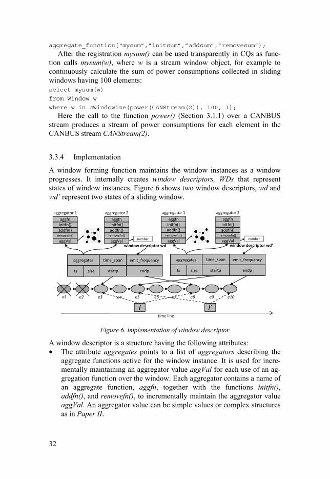
A window forming function maintains the window instances as a window progresses. It internally creates window descriptors, WDs that represent states of window instances. Figure 6 shows two window descriptors, wd and wd’ represent two states of a sliding window.
Figure 6. implementation of window descriptor
A window descriptor is a structure having the following attributes: • The attribute aggregates points to a list of aggregators describing the
aggregate functions active for the window instance. It is used for incre-mentally maintaining an aggregator value aggVal for each use of an ag-gregation function over the window. Each aggregator contains a name of an aggregate function, aggfn, together with the functions initfn(), addfn(), and removefn(), to incrementally maintain the aggregator value aggVal. An aggregator value can be simple values or complex structures as in Paper II.
aggregates
size
time_span
ts
emit_frequency
startp endp
initfn()addfn()
removefn()
aggfn
aggVal
time line
aggregates
size
time_span
ts
emit_frequency
startp endp
initfn()addfn()
removefn()
aggfn
aggVal
initfn()addfn()
removefn()
aggfn
aggVal number
aggregator 1 aggregator 2aggregator 1
window descriptor wd
e1 e2 e3 e4 e6e5 e7 e8 e9 e10
l l’
initfn()addfn()
removefn()
aggfn
aggVal number
aggregator 2
window descriptor wd’

33
• If the elements are time stamped, the attribute time_span is computed as the difference between the time stamps of the last and first elements of the list of stream elements, the element list, required to maintain the window kind. Notice that the time span of a time window instance may be smaller than the window size specified by its window forming func-tion.
• If the window is a FEW window, the emit frequency specifies the emit rate.
• The time stamp of the window is stored in attribute ts. It is omitted for windows that are not time stamped.
• Attribute size is the number of elements in the window extent. • Continuously arriving stream elements are added by the window form-
ing function to the element list. The element list is represented by startp and endp pointers that point to its first and last stream element, respec-tively. When new elements are received by the window forming function they are added to the end.
Maintaining window instances Figure 6 illustrates a situation where elements e1 – e10 have arrived to a window forming function. There are two window instances described by the window descriptors wd and wd’ having the element lists l and l’, respec-tively. The elements e5 – e8 are shared between the two element lists. After a window descriptor has been emitted, a new window descriptor is created where all properties are modified in order to represent the new state of the progressed window. The old descriptor is not updated so that references to it from other system objects (e.g. parent windows) can still use the old state. In the figure a window instance wd has been emitted and wd’ is formed. Old stream elements stay in memory when there are at least one window descrip-tors referencing them; otherwise an incremental garbage collector frees them. In the figure, e1 and e2 are freed because they are not referenced by other objects.
SVALI allows separating window emits not only when the window is full but also before that, as required by FEW windows. For a FEW window with size sz, stride st, and emit frequency ef, an early emit happens every ef units without considering whether the window has reached the size sz or not. Early emitted windows are partial windows of the complete window, i.e. the ele-ment lists of the early emitted windows will have the same start pointers startp but different end pointers endp. A final emit happens only when the window is full where the window has the full size sz. After the complete window has been emitted, the window progresses forward with stride st, i.e. the start pointer startp of the element list moves forward with stride st.
Maintaining window aggregates New aggregate functions are registered to a window descriptor dynamically when the aggregate function is called for the window instance the first time.

34
When a window is formed there are no aggregators; instead they are dy-namically added by the aggregate functions. The approach is flexible, pro-vides incremental evaluation of aggregate functions, and maintains old ver-sions of each window instance as it slides. It is interfaced with an incre-mental garbage collector that removes expired elements and window de-scriptors no longer referenced. Windows can be nested to arbitrary levels.
The following pseudo-code illustrates how an aggregate function aggfn() is implemented with a window descriptor wd as parameter:
aggfn(wd):
wd is a window descriptor
if aggfn is registered on wd then
return aggVal of aggfn in wd
else
register aggfn to wd
calculate aggVal for wd
by first calling aggfn.initfn()
and then calling aggfn.addfn() for each element in wd
return aggVal;
The window forming functions implement the incremental evaluation as new stream elements arrive and old expire. The following pseudo-code shows how windows are maintained incrementally for time based, count based, and FEW sliding and tumbling windows:
window_former(s, sz, st):
s is a handle to the incoming stream
sz is the size of the window
st is the stride of the window
wd is a new window descriptor
for each arrived stream element e in s
add e to the of the element list of wd
increment wd.endp and wd.size
for each aggfn registered with wd
aggfn.addfn(e, aggVal); //add the contribution of e if wd is FEW window then emit wd wd = copy_descriptor(wd) else if wd.size == sz then emit wd
wd = copy_descriptor(wd)
move wd.startp st steps forward
for each expired element es
for each aggfn in wd
aggfn.removefn(es, aggVal)//remove the contribution
35
The function copy_descriptor(wd) copies the window descriptor and its aggregators but not the element list. Thus, a new window instance is created when the window progresses without updating old instances, providing mul-tiple versions of window instances.
Defining a new window types is done by making new window forming functions. For example, for predicate and partition windows the window forming functions maintain the element list by calling user functions rather than using sz and st. The pseudo code for predicate and partitions windows is in http://www.it.uu.se/research/group/udbl/SVALIWindows.pdf
3.4 Data Stream Validation In order to detect unexpected equipment behaviour, a validation model de-fines the correctness of a kind of equipment by a set of validation functions, which for each validated stream from the equipment produces a validation stream describing the differences between measured and expected measure-ments. The validation model is stored as meta-data in the local database. Each tuple in a validation stream has the format (ts, mv, x, …) where ts is the time of the measurement, mv is the measured value, and x is the expected value. In addition, application dependent values describing the anomaly are included in each validation stream element. For example, a CANBUS stream contains measurements of different kinds, so the validation stream elements include an identifier of the anomaly, called a signal identifier. The validation models can also produce alert streams, whose elements are time stamped error messages describing the detected anomalies. Empty strings indicate normal behaviour.
The validation functions can be executed per received element to test for anomalies. This kind of validation is called instant validation. A simple ex-ample of this kind is, “The temperature of functioning equipment should not exceed 90°C”.
Some monitoring is based on stream windows rather than individual stream elements. In SVALI this is naturally handled since the result of a window forming function is a stream of windows. For example, manufactur-ing often is cyclic since the same behavior is repeated for each manufactured item. Monitoring manufacturing cycles sometimes is more meaningful than instant validations of the measurements during the cycle. This kind of vali-dation requires the validation models to be built based on stream windows and is called window validation. For example, instead of validating the tem-perature of the equipment for each time interval, the moving average of the temperature during each manufacturing cycle is checked. The manufacturing cycle is defined as predicate windows indicating when a manufacturing tool is active.

36
3.4.1 Model-and-validate
The expected value can be estimated based on a physical model, which pro-duces expected values based on physical properties of the monitored equip-ment. Physical models are defined as user defined functions that map meas-ured parameters to the monitored variables. To detect anomalies, each ele-ment of a received stream is checked against the physical model of the equipment stored as a validation model in the local database. For example, in Paper III a mathematical model is developed estimating the expected normal power usage based on sensor readings in stream elements. The mathematical model is expressed as derived functions and installed in SVALI’s local data-base. The system provides a general function, called model_n_validate(), which compares data elements in CQs with the installed physical model and emits a validation stream of significant deviations. It has the following sig-nature: model_n_validate(Bag of Stream s, Function modelfn,
Function validate fn)
-> Stream of (Number ts, Object m, Object x, …)
The second input parameter, modelfn(Object r, ...) -> Object x, is a func-tion defining the physical model where an expected value x is defined in terms of a received stream element r. The received stream element r can be, e.g., a number, a vector, or a window. The expected value x can be a single value or a collection of values specifying allowed properties of r. In particu-lar, if r is a window containing many measurements, x can be a set of al-lowed values. The function validatefn(Object r, Object x, ...) -> Bag of (Number ts, Charstring mid, Object m) specifies whether a received stream element r is invalid compared to the expected value x as computed by the model function. In case r is invalid the validation function returns a set of tuples (ts, mid, m) representing the time of each invalid measurement m named mid detected in r. The model function can also be a stored function populated by, e.g., mining historical data. In that case the reference model is first mined offline and the computed parameters explicitly stored in the stored function modelfn() passed to model_n_validate().
CQ specifications involving model-and-validate calls are sent to a SVALI server as a text string for dynamic execution. It is up to the SVALI server to determine how to execute the CQs in an efficient way.
3.4.2 Learn-and-validate
In cases where a mathematical model of the normal behavior is not easily obtained the system provides an alternative validation mechanism to learn the expected behavior by dynamically building a statistical reference model based on sampled normal behavior measured during the first n stream ele-ments in a stream. Once the reference model has been learned it is used to

37
validate the rest of the stream. This is called learn-and-validate and is im-plemented by a stream function with the following signature: learn_n_validate(Bag of Stream s, Function learnfn, Integer n,
Function validatefn)
-> Stream of (Number ts, Object m, Object x, …)
The learning function, learnfn(Vector of Object f)->Object x, specifies how to collect statistics x as a reference model of the expected behavior, based on a sequence f of the n first streams elements.
As for model-and-validate, the validation function, validatefn(Object r, Object x, …)-> Bag of (Number ts, Charstring mid, Object m), returns a set of tuples (ts, mid, m) whenever a measured value m named mid in r is invalid at time ts compared to the reference value x returned by the learning func-tion.
The function learn_n_validate() returns a validation stream of tuples (ts, m, x) with time stamp ts, measured value m, and the expected value x accord-ing to the reference model learned from the first n normally behaving stream elements.
In Paper III learn-and-validate is used to validate drill cycles.
38
4 Technical Contributions
Details of the technical contributions of the thesis are described by the re-search papers below. Short summaries of the research questions covered in each paper are as follows.
4.1 Paper I C. Xu, E. Källström, T. Risch, J. Lindström, L. Håkansson, and J. Larsson: Scalable Validation of Industrial Equipment using a Functional DSMS, sub-mitted for journal publication, 2016.
Summary
In Volvo Construction Equipment, clutch failures may lead to unnecessary costs of expensive downtime and maintenance of construction equipment machines. An efficient solution is to apply data mining algorithms such as feature extraction and classification methods on data streams from sensors on-board. The functional model of the DSMS SVALI is used to define meta-data about the equipment at Volvo CE. The anomaly detection models over raw numerical data streams are defined in terms of the meta-data model. To monitor machines that are geographically distributed, SVALI can start up many peers, where at each site customized CQs are installed. The validation CQs are defined using model-and-validate.
For security reasons the monitored machines are located behinds fire-walls, i.e. raw data streams are protected. The stream uploader module makes it possible for on-board SVALI peers to transmit transformed and filtered data streams to the monitoring server.
In the paper the number of machines to be monitored, the rate of each streams, and the number of CQs are scaled to investigate the scalability of the system with respect to system throughput and response time.
The paper partly answers research question two by using a partition win-dow to capture gearshifts of wheel loaders. It further answers research ques-tion three and four.

39
I am the primary author of this paper. This work is based on a real SVALI installation at Volvo CE. The other authors contributed to algorithm devel-opment, discussions, and paper writing.
4.2 Paper II S. Badiozamany, L. Melander, T. Truong, C. Xu, and T. Risch: Grand Chal-lenge: Implementation by Frequently Emitting Parallel Windows and User-Defined Aggregate Functions, Proc. The 7th ACM International Conference on Distributed Event-Based Systems, DEBS 2013, Arlington, Texas, USA, June 29 - July 3, 2013.
Summary
We implemented the grand challenge of DEBS using SVALI. The data from this challenge is generated from a number of sensors installed on shoes of the participants and the football of a soccer game. The rate of the data from the shoes is 200 HZ and from the football 2000 HZ. The challenge is to an-swer four CQs in real time: (Q1) running analysis, (Q2) ball possessions, (Q3) heat map computations, and (Q4) detecting shots on goal. To be able to return results within required time limit, the new window type FEW (fre-quency emitting window) was developed, where partial windows are re-turned to downstream operators. FEW windows are necessary when the re-sult from a window computation must be emitted before the full window is formed when the window slides.
In our implementation, the computation is significantly simplified and improved by incremental evaluation of window aggregations. By defining initfn(), addfn(), and removefn(), user defined incremental aggregation func-tions can be registered on windows dynamically.
The paper partly answers research question two with the window type FEW. It partly answers research question four by showing the scalability of the system.
I implemented the FEW window type and the user defined incremental window aggregations. I fully implemented Q3 and partly implemented Q1 and Q2. I am also responsible for setting up the overall execution data stream flow. The other authors contributed to query implementation, discus-sions, and paper writing.

40
4.3 Paper III C. Xu, D. Wedlund, M. Helgoson, and T. Risch: Model-based Validation of Streaming Data, The 7th ACM International Conference on Distributed Event-Based Systems, DEBS 2013, Arlington, Texas, USA, June 29 - July 3, 2013.
Summary
In the Sandvik scenario, it has been identified that suitable combination of cutting tools, process parameters, machine tools and cutting strategies will support efficient manufacturing of parts leading to less power consumption.
In some cases, the monitoring can be done by a physical model estimating the power consumption based on sensor measurements, i.e. model-and-validate. In other cases no pre-defined model can be built, instead the model is learnt by collecting statistics of normally behaving machines of the same kind, i.e. learn-and-validate. The paper shows that when scaling the number of monitored machines the validation can still meet the real time requirement by parallel stream processing.
The paper partly answers research question two by proposing predicate windows that capture the cyclic behavior of streams from manufacturing equipment. The validation functionalities and the experiments partly answer research question three and four.
I am the primary of this paper. The work is based on a real application from Sandvik Coromant. The other authors contributed to the discussions and paper writing.

41
5 Conclusions and Future Work
In this thesis, the SVALI system is presented, which is a DSMS to analyze streams in order to detect anomalies in monitored equipment. Anomalies in the behavior of heavy-duty equipment streams are detected by running SVALI on-board the machines. Anomaly detection rules are expressed de-claratively as continuous queries over mathematical or statistical models that match incoming streamed sensor readings against an on-board database of normal readings.
To process high volume data streams, SVALI includes a set of stream window forming functions, such as time windows and count windows. To support the industrial application domain three new window types have been added: predicate windows, partition windows, and FEW windows along with a mechanism to dynamically plug-in user defined incremental aggregate functions over windows.
To enable scalable validation of geographically distributed equipment, SVALI is a distributed system where many SVALI instances can be started and run in parallel on the equipment. Central analyses are made in a moni-toring center where streams of detected anomalies are combined and ana-lyzed on a cluster.
The functional data model of SVALI provides definition of meta-data and validations models in terms of typed functions. Continuous queries are ex-pressed declaratively in terms of functions where streams are first class ob-jects. Furthermore, SVALI is an extensible system where functions can be implemented using external libraries written in C, Java, and Python.
To control the transmission of equipment data streams to the monitoring center data streams from the equipment are transmitted to the monitoring center using a stream uploader.
To enable stream validation on a high level, the system provides two sys-tem validation functions, model_n_validate() and learn_n_validate(). model_n_validate() allows the user to define mathematical models based on physical properties of the equipment to detect unexpected deviations of val-ues in stream elements. The model can also be built using historical data and then stored in the database as reference model. By contrast, learn_n_validate() builds statistical model by sampling the stream online as it flows. The model can also be re-learnt in order to keep updated, e.g. after every time units or amount of stream elements.

42
Experimental results show that the distributed SVALI architecture enable scalable monitoring and anomaly detection with low response times when the number of monitored machines and their data stream rates increase. The experiments were made using real data recorded in running equipment. The experiments show that parallel validation where expensive computations are done in the local SVALI peers enables fast response time and high through-put.
One direction of future work is to have more complicated joins of differ-ent kinds of data streams from different equipment exploring more informa-tion about the streams. New scalability challenges may come up w.r.t. paral-lel stream joins and distribution of data stream operators. Another direction is to analyze parallelization strategies when there are shared computations between CQs over the same data stream. For example, in SVALI, the model and validation functions of model_n_validate() and learn_n_validate() may have overlapping definitions and it is worth exploring parallel shared com-putations between different validation CQs.
In SVALI, different windows are created by a set of window forming functions. We plan to continue exploring the window semantics to have a more general way to define and extend new stream windows. Putting index over stream windows is also an interesting future work.
43
6 Summary in Swedish
Traditionella databashanteringssystem (DBMS) som Oracle, SQL Server och MySQL lagrar data som permanenta tabeller på disk. Användaren kan sedan specificera frågor uttryckta i ett frågespråk för att göra sökningar över tabel-lerna som de ser ut vid frågetillfället. Denna modell är utmärkt för många vanliga databastillämpningar, till exempel för kontohantering i banktillämp-ningar.
Under senare år genererar många system data i realtid, vilket inte passar in i den traditionella modellen. Det gäller t.ex. för aktiehandel, trafiköver-vakning och sensorer på maskiner. Dessa system genererar data i realtid som dataströmmar av mätvärden, ofta med mycket hög volym per tidsenhet, kan-ske megabytes eller gigabytes per sekund, vilket gör det opraktiskt eller t.o.m. omöjligt att först lagra data på disk och sedan söka i data som i den traditionella modellen. Dessutom kräver moderna beslutstöd- och produk-tionssystem mycket snabb respons när verkligheten ändras så den fördröj-ning som orsakas av att först lagra och sedan söka data kan vara oacceptabel. Till exempel att övervaka tillståndet hos olika komponenter i industriella maskiner kräver att systemet kan reagera snabbare än en sekund. För att stödja den sortens tillämpningar har en ny typ av system utvecklats under senare år, så kallade dataströmhanteringssystem (DSMS), t.ex. AURORA [2], STREAM [8] och i Uppsala SCSQ [69]. Sökningar över strömmar speci-ficeras som kontinuerliga frågor (eng. continuous queries, CQs) eftersom de körs kontinuerligt tills de explicit avslutas och producerar kontinuerligt en dataström som resultat under tiden de är aktiva. Eftersom dataströmmar ofta är mycket långa eller t.o.m. oändliga görs bearbetningen ofta över bara de senast anlända mätvärdena i strömmen, så kallade strömfönster.
För att industriell utrustning såsom lastmaskiner och tillverkningssystem skall kunna leverera en högkvalitativ service krävs att utrustningen kontinu-erligt övervakas för att upptäcka och förutse fel. Allteftersom utrustningen blir mer komplex investeras mer och mer FoU i att automatiskt upptäcka onormalt beteende hos maskiner [55]. Till exempel har Volvo Construction Equipment (VCE) installerat sensorer på sina L90F frontlastare för att över-vaka tillståndet hos transmissionen. Data levereras från dessa sensorer via CANBUS-protokollet, vilket är en standard för dataöverföring i realtid från olika sorters maskiner. Relativt dyrbara statistiska analyser i realtid krävs för att upptäcka och förutse onormalt beteende och att vidta åtgärder snabbt för att reducera underhållskostnaden. När antalet övervakade maskiner blir stort,

44
t.ex. 10000, blir det vidare viktigt att bearbetning skalar upp och fortfarande kan utföras med korta fördröjningar.
Med den ansats som förslås i denna avhandling ses validering av maski-nell utrustning som en speciell sorts kontinuerliga frågor som analyserar strömmar från sensorer i termer av matematiska modeller och data lagrade i en lokal databas inuti dataströmhanteringssystemet. Följande forskningsfrå-gor behandlas i avhandlingen:
1. Den övergripande forskningsfrågan är: Hur bör ett dataströmhanter-ingssystem designas för att möjliggöra skalbar validering av indust-riell utrustning?
2. Vilka sorters strömfönster behöver systemet tillhandahålla för skal-bar validering av strömmar av mätvärden?
3. Vilken sorts mekanismer behövs för att specificera validering av da-taströmmar på hög nivå?
4. Hur kan skalbar och effektiv dataströmvalidering implementeras? För att besvara den första forskningsfrågan, har ett system som heter SVALI (Stream VALIdator) utvecklats och som utvärderats för verkliga industriella tillämpningar. Paper I beskriver SVALIs övergripande arkitektur och visar hur det använts i praktiken för att upptäcka onormalt beteende hos industriell utrustning i bruk.
Paper II presenterar olika sorters strömfönster och visar hur de är väl lämpade för dataanalys i realtid, tillämpat på realtidsdata från verkliga fot-bollsmatcher. Speciellt presenteras FEW-fönster som producerar strömman-de mätvärden redan innan fullständiga fönster är klara. Användardefinierade aggregeringsfunktioner tillåter kontinuerlig strömmande leverans av statis-tiska och andra sorters resultat. De nya typer av strömfönster som krävs för industriell övervakning presenteras i Paper III. Behovet av olika sorters strömfönster har lett till utvecklandet av en utbyggbar strömfönstermeka-nism i SVALI där användaren kan plugga in nya sorters strömfönster vid behov. Detta besvarar den andra forskningsfrågan.
SVALI tillhandahåller två speciella systemfunktioner model-and-validate och learn-and-validate för att specificera på en hög användarnivå kontinuer-liga frågor uttryckta i termer av valideringsmodeller, som behandlas i Paper I och Paper II. Valideringsmodellerna uttrycks som matematiska formler över strömmande mätvärden. För utrustning där det är svårt eller omöjligt att definiera en fysisk modell kan systemet i stället lära sig normalt uppträdande genom att övervaka normalt fungerande utrustning i realtid under en trä-ningsperiod. Detta besvarar den tredje forskningsfrågan.
Prestanda hos funktioner för att skapa strömfönster med användardefinie-rade aggregeringsfunktioner utvärderas i Paper II. Prestanda och skalbarhet av parallellt exekverande valideringsfunktioner utvärderas i Paper III. Detta besvarar den fjärde forskningsfrågan.

45
7 Acknowledgements
First and foremost I would like to thank my supervisor professor Tore Risch. Thank you for letting me pursue PhD here in the UDBL group. Thank you for guiding my way throughout my studies, and for sharing your knowledge with me during the discussions. I am thankful for the advanced database course that you gave in the first year. I learned a lot during my stay. I en-joyed the time we travelled together to Sandviken, Eskilstuna, Frankfurt, and Luxembourg. I also appreciate your patience to help me with the technical implementations and scientific writing.
I am grateful to meet former and current UDBL members, Kjell Orsborn, Erik Zeitler, Ruslan Fomkin, Gyozo Gidofalvi, Manivasakan Sabesan, Silvia Stefanova, Lars Melander, Minpeng Zhu, Andrej Andrejev, Robert Kajic, Thanh Truong, Mikael Lax, Sobhan Badiozamany, and Khalid Mahmood. I would like to thank Kjell Orsborn, Silvia Stefanova, and Manivasakan Sabe-san for helping me being the assistant of the Database Technology courses for the first time. I had the pleasure to share the office with Andrej, Robert, Mikael, and Lars. I had a good time talking to you both academically and non-academically. Thank you Minpeng, as the only two Chinese PhDs in the group, thank you for the discussions you shared with me and the help you gave me in various aspects of my life. Thank you Lars, I enjoyed the time when we did the project together for the demonstration. Thank you Lars, Thanh, and Sobhan, I am lucky to have you as a team to do the grand chal-lenge together. I miss those times!
I would like to thank Matteo Magnani. I like your ways of conducting courses, not to mention the parties you held in house 17.
Ulrika Andersson deserves a special mention. I really appreciate the ad-vices and assistance you provided, e.g. for certificate needed for visa exten-sion every year, and for the housing suggestions when I have nowhere to live, and many more.
I would like to thank Liying Zheng, thank you for bringing me all those happiness and sadness moments. I missed the time we travel around together and sent post cards to each other. I also would like to thank my friend Yong Huang and his significant other Jinyan Liu. I am thankful to have you as my flat mate in the first two years of my studies. You are like my big brother, thank you for your fruitful comments of my research and for being there when I had ups and downs.

46
Big thanks to the friends in Uppsala, I am really happy to know all of you, and because of you I do not feel lonely abroad. Thank you, Wanjun Chu (褚爸爸), Yingjie Chen, Fangming Lan (兰胖子), Beichen Xie, Weihua Lan (小包子), Weixian Wu (吴小神), Yu Liu, Mi Wang and Meng Liang. I en-joyed the get-togethers and the great food from all of you. The BMC Chi-nese group also needs a special mention, Yue Cui, Lu Lu, Yani Zhao, Lei Chen, Hua Huang, Hui Xu, Zhoujie Ding, Junhong Yan, Lu Zhang, Zhirong Fu, Rui Di, Chaoying Lin, Xiaohu Guo, Kai Hua, Jin Zhao, Ziquan Yu, and Wangsu Jiang. Although we do not share the same research topics, we share a lot in other aspects of my life. Lu Lu, thank you for letting me in when I feel lost.
Before I came to Uppsala University, I did my master in Chalmers Uni-versity of Technology. I am happy to meet Yongyang Yu, Xingxing Liu, Ning He, Yue Wu, Cankun Zhang, Xing Lan, Yefeng Liu, and Jing Wen. Thank you Cankun for being my master thesis project partner, and for en-couraging me to look for a better self. Yefeng Liu, Jing Wen and Xing Lan, thank you for your companies throughout my master and PhD studies, be-cause of you I feel I am not the only one.
Basketball has always being my favorite sport and the best way of relax-ing. I am thankful to be part of the basketball group in Uppsala. I like the feeling when we had something to fight for together.
I am really grateful to my family for the encouragement and the support. As in a Chinese saying, “You should not go abroad when you have a family. If you do, you should go to a fixed place and go for a reason!” (父母在, 不远游, 游必有方), I am thankful for the freedom and the patience you gave me during all these years abroad. Thank you!!!
Cheng Xu 徐程
This project is supported by EU FP7 Project Smart Vortex, the Swedish Foundation for Strategic Research, and eSSENCE under contract RIT08-0041.
47
Bibliography
1. Abadi, D. J., Ahmad, Y., Balazinska, M., Cherniack, M., Hwang, H. J., Lindner, W., Maskey, A. S., Rasin, E., Ryvkina, E., Tatbul, N., Xing, Y., Zdonik, S.: The Design of the Borealis Stream Processing Engine. Proc. CIDR 2005.
2. Abadi, D. J., Carney, D., Cetintemel, U., Cherniack, M., Convey, C., Lee, S., Stonebraker, M., Tatbul, N., Zdonik, S.: Aurora: A New Model and Architec-ture for Data Stream Management. The VLDB Journal 12(2), 120 - 139 (2003).
3. Al-Kateb, M., and Lee, B. S.: Load Shedding for Temporal Queries over Data Streams. Journal of Computing Science and Engineering, Volume 5, Number 4, pp.294-304 (2011).
4. Amazon Kinesis. https://aws.amazon.com/kinesis/streams/ 5. Angiulli, F., Fassetti, F.: Distance-based Outlier Queries in Data Streams: The
Novel Task and Algorithms. Journal of Data Mining and Knowledge Discovery, 20(2), 290 - 324 (2010).
6. Apache Flink. https://flink.apache.org/ 7. Apache Storm. http://storm.apache.org/ 8. Arasu, A., Babcock, B., Babu, S., Cieslewicz, J., Datar, M., Ito, K., Motwani,
R., Srivastava, U., Widom, J.: STREAM: The Stanford Data Stream Manage-ment System. Technical Report 2004-20, Stanford InfoLab (2004).
9. Arasu, A., Cherniack, M., Galvez, E., Maier, D., Maskey, A. S., Ryvkina, E., Stonebraker, M., and Tibbetts, R.: Linear Road: A Stream Data Management Benchmark. Proc. VLDB 2004.
10. Arasu, A., Babu, S., Widom, J.: The CQL Continuous Query Language: Seman-tic Foundations and Query Execution. Technical Report 2003-67, Stanford In-foLab (2003).
11. Arasu, A., Widom, J.: A Denotational Semantics for Continuous Queries over Streams and Relations. SIGMOD Record, 33(3), 6 - 11 (2004).
12. Arasu, A., Widom, J.: Resource Sharing in Continuous Sliding-window Aggre-gates. Proc. VLDB 2004.
13. Avnur, R., Hellerstein, J. M.: Eddies: Continuously Adaptive Query Processing. SIGMOD Record, 29(2), 261 - 272 (2000).
14. Babcock, B., Babu, S., Datar, M., Motwani, R., Thomas, D.: Operator Schedul-ing in Data Stream Systems. The VLDB Journal, 13(4), 333 - 353 (2004).
15. Babcock, B., Datar, M., Motwani, R.: Load Shedding for Aggregation Queries over Data Streams. Proc. ICDE 2004.
48
16. Babu, S., Motwani, R., Munagala, K., Nishizawa, I., Widom, J.: Adaptive Or-dering of Pipelined Stream Filters. Technical Report 2003-69, Stanford InfoLab (2003).
17. Bai, Y., Thakkar, H., Wang, H., Luo, C., Zaniolo, C.: A Data Stream Language and System Designed for Power and Extensibility. Proc. CIKM 2006.
18. Botan, I., Derakhshan, R., Dindar, N., Haas, L., Miller, R.J., Tatbul, N.: Secret: A Model for Analysis of the Execution Semantics of Stream Processing Sys-tems. Proc. VLDB 2010.
19. Botan, I., Kossmann, D., Fischer, P. M., Kraska, T., Florescu, D., Tamosevicius, R.: Extending XQuery with Window Functions. Proc. VLDB 2007.
20. Brenna, L., Demers, A., Gehrke, J., Hong, M., Ossher, J., Panda, B., Riedewald, M., Thatte, M., White, W.: Cayuga: A High-performance Event Processing En-gine. Proc. SIGMOD 2007.
21. CANBUS. http://en.wikipedia.org/wiki/CAN_bus 22. Cao, H., Zhou, Y., Shou, L., Chen, G.: Attribute Outlier Detection over Data
Streams. Proc. DASFAA 2010. 23. Cao, L., Wang, Q., Rundensteiner, E. A.: Interactive Outlier Exploration in Big
Data Streams. Proc. VLDB 2014. 24. Carney, D., Cetintemel, U., Cherniack, M., Convey, C., Lee, S., Seidman, G.,
Stonebraker, M., Tatbul, N., Zdonik, S.: Monitoring Streams: A New Class of Data Management Applications. Proc. VLDB 2002.
25. Carney, D., Cetintemel, U., Rasin, A., Zdonik, S., Cherniack, M., Stonebraker, M.: Operator Scheduling in a Data Stream Manager. Proc. VLDB 2003.
26. Chandrasekaran, S., Cooper, O., Deshpande, A., Franklin, M.J., Hellerstein, J.M., Hong, W., Krishnamurthy, S., Madden, S., Raman, V., Reiss, F., Shah, M.: TelegraphCQ: Continuous Data Flow Processing for an Uncertain World. Proc. CIDR 2003.
27. Chen, J., DeWitt, D.J., Tian, F.,Wang, Y.: NiagaraCQ: A Scalable Continuous Query System for Internet Databases. Proc. SIGMOD 2000.
28. Cherniack, M., Balakrishnan, H., Balazinska, M., Carney, D., Cetintemel, U., Xing, Y., Zdonik, S.: Scalable Distributed Stream Processing. Proc. CIDR 2003.
29. Chui, C.K., Kao, B., Lo, E., Cheung, D.: S-OLAP: An OLAP System for Ana-lyzing Sequence Data. Proc. SIGMOD 2010.
30. Cranor, C., Johnson, T., Spataschek, O., Shkapenyuk, V.: Gigascope: A Stream Database for Network Applications. Proc. SIGMOD 2003.
31. Datar, M., Gionis, A., Indyk, P., Motwani, R.: Maintaining Stream Statistics over Sliding Windows. Proc. SODA 2002.
32. Demers, A., Gehrke, J., P, B.: Cayuga: A General Purpose Event Monitoring System. Proc. CIDR 2007.
33. Georgiadis, D., Kontaki, M., Gounaris, A., Papadopoulos, A.N., Tsichlas, K., Manolopoulos, Y.: Continuous Outlier Detection in Data Streams: An Extensi-ble Framework and State-of-the-art Algorithms. Proc. SIGMOD 2013.
49
34. Ghanem, T.M., Aref, W.G., Elmagarmid, A. K.: Exploiting Predicate Window Semantics over Data Streams. SIGMOD Record 35(1), 3 - 8 (2006).
35. Ghanem, T.M., Elmagarmid, A.K., Larson, P. A., Aref, W. G.: Supporting Views in Data Stream Management Systems. ACM Trans. Database Syst. 35(1), 1:1 - 1:47 (2008).
36. Girod, L., Mei, Y., Newton, R., Rost, S., Thiagarajan, A., Balakrishnan, H., Madden, S.: The Case for a Signal-Oriented Data Stream Management System. Proc. CIDR 2007.
37. Girod, L., Mei, Y., Rost, S., Thiagarajan, A., Balakrishnan, H., Madden, S.: XStream: A Signal-Oriented Data Stream Management System. Proc. ICDE 2008.
38. Jain, N., Mishra, S., Srinivasan, A., Gehrke, J., Widom, J., Balakrishnan, H., Cetintemel, U., Cherniack, M., Tibbetts, R., Zdonik, S.: Towards a Streaming SQL Standard. Proc. VLDB 2008.
39. Katchaounov, T. Josifovski, V., and Risch, T.: Scalable View Expansion in a Peer Mediator System. Proc. DASFAA 2003.
40. Kazemitabar, S.J., Demiryurek, U., Ali, M., Akdogan, A., Shahabi, C.: Geospa-tial Stream Query Processing using Microsoft SQL Server StreamInsight. Proc. VLDB 2010.
41. Kontaki, M., Gounaris, A., Papadopoulos, A.N., Tsichlas, K., Manolopoulos, Y.: Continuous Monitoring of Distance-based Outliers over Data Streams. Proc. ICDE 2011.
42. Krishnamurthy, S., Chandrasekaran, S., Cooper, O., Deshpande, A., Franklin, M.J., Hellerstein, J. M., Hong, W., Madden, S., Reiss, F., Shah, M. A.: Tele-graphCQ: An architectural Status Report. IEEE Data Engineering Bulletin 26(1), 11 - 18 (2003).
43. Li, J., Maier, D., Tufte, K., Papadimos, V., Tucker, P.A.: No Pane, no Gain: Efficient Evaluation of Sliding Window Aggregates over Data Streams. Proc. SIGMOD 2005.
44. Li, J., Maier, D., Tufte, K., Papadimos, V., Tucker, P.A.: Semantics and Evalua-tion Techniques for Window Aggregates in Data Streams. Proc. SIGMOD 2005.
45. Madden, S., Franklin, M.J.: Fjording the Stream: An Architecture for Queries over Streaming Sensor Data. Proc. ICDE 2002.
46. Maier, D., Li, J., Tucker, P., Tufte, K., Papadimos, V.: Semantics of Data Streams and Operators. Proc. ICDT 2005.
47. Munagala, K., Srivastava, U., Widom, J.: Optimization of Continuous Queries with Shared Expensive Filters. Proc. SIGMOD 2007.
48. Naughton, J., Dewitt, D., Maier, D., Aboulnaga, A., Chen, J., Galanis, L., Kang, J., Krishnamurthy, R., Luo, Q., Prakash, N., Ramamurthy, R., Shanmugasunda-ram, J., Tian, F., Tufte, K., Viglas, S.: The Niagara Internet Query System. IEEE Data Engineering Bulletin 24, 27 - 33 (2001).
50
49. Olston, C., Jiang, J., Widom, J.: Adaptive Filters for Continuous Queries over Distributed Data Streams. Proc. SIGMOD 2003.
50. Patroumpas, K. and Sellis, T.: Window Specification over Data Streams. Proc. EDBT 2006.
51. Petit, L., Labbe, C., Roncancio, C. L.: An Algebraic Window Model for Data Stream Management. Proc. MobiDE 2010.
52. Plagemann, T., Goebel, V., Bergamini, A., Tolu, G., Urvoy-Keller, G., Bier-sack, E. W.: Using Data Stream Management Systems for Traffic Analysis - A Case Study. Proc. PAM 2004.
53. Raman, V., Deshpande, A., Hellerstein, J. M.: Using State Modules for Adap-tive Query Processing. Proc. ICDE 2003.
54. Sadik, S. and Gruenwald, L.: Research Issues in Outlier Detection for Data Streams. ACM SIGKDD Explorations Newsletter, vol. 15, no. 1, pp. 33 – 40 (2014).
55. Setu, M. N., Mark, W., Shunsuke, C., Liu, Q., Kihoon, C. and Krishna, P.: Sys-tematic Data-Driven Approach to Real-Time Fault Detection and Diagnosis in Automative Engines. IEEE Autotestcon, pp. 59 – 65 (2006).
56. Shah, M.A., Chandrasekaran, S., Hellerstein, J.M., Ch, S., Franklin, M. J.: Flux: An Adaptive Partitioning Operator for Continuous Query Systems. Proc. ICDE 2002.
57. Smart Vortex Project. http://www.smartvortex.eu/ 58. Spark Streaming. http://spark.apache.org/streaming/ 59. Srivastava, U., Munagala, K., Widom, J.: Operator Placement for in-network
Stream Query Processing. Proc. SIGMOD 2005. 60. StreamBase. http://www.streambase.com/ 61. Subramaniam, S., Palpanas, T., Papadopoulos, D., Kalogeraki, V., Gunopulos,
D.: Online Outlier Detection in Sensor Data using Non-parametric Models. Proc. VLDB 2006.
62. Tatbul, N., Cetintemel, U., Zdonik, S., Cherniack, M., Stonebraker, M.: Load Shedding in a Data Stream Manager. Proc. VLDB 2003.
63. Tatbul, N., Zdonik, S.: Window-aware Load Shedding for Aggregation Queries over Data Streams. Proc. VLDB 2006.
64. Tian, F., DeWitt, D. J.: Tuple Routing Strategies for Distributed Eddies. Proc. VLDB 2003.
65. Xing, Y., Zdonik, S., Hwang, J. H.: Dynamic Load Distribution in the Borealis Stream Processor. Proc. ICDE 2005.
66. Xu, W., Bodik, P., Patterson, D.: A Flexible Architecture for Statistical Learn-ing and Data Mining from System Log Streams. Proc. Temporal Data Mining: Algorithms, Theory and Applications 2004.
67. Yang, D., Rundensteiner, E. A.,Ward, M. O.: Neighbor-based Pattern Detection for Windows over Streaming Data. Proc. EDBT 2009.
68. Ye, H., Kitagawa, H., Xiao, J.: Continuous Angle-based Outlier Detection on High Dimensional Data Streams. Proc. IDEAS 2014.

51
69. Zeitler, E., Risch, T.: Massive Scale-out of Expensive Continuous Queries. Proc. VLDB 2011.
70. Zhang, J., Gao, Q., Wang, H.: Spot: A system for Detecting Projected Outliers from High Dimensional Data Streams. Proc. ICDE 2008.
71. Zhu, Y., Rundensteiner, E.A., Heineman, G. T.: Dynamic Plan Migration for Continuous Queries over Data Streams. Proc. SIGMOD 2004.

Acta Universitatis UpsaliensisDigital Comprehensive Summaries of Uppsala Dissertationsfrom the Faculty of Science and Technology 1384
Editor: The Dean of the Faculty of Science and Technology
A doctoral dissertation from the Faculty of Science andTechnology, Uppsala University, is usually a summary of anumber of papers. A few copies of the complete dissertationare kept at major Swedish research libraries, while thesummary alone is distributed internationally throughthe series Digital Comprehensive Summaries of UppsalaDissertations from the Faculty of Science and Technology.(Prior to January, 2005, the series was published under thetitle “Comprehensive Summaries of Uppsala Dissertationsfrom the Faculty of Science and Technology”.)
Distribution: publications.uu.seurn:nbn:se:uu:diva-291530
ACTAUNIVERSITATIS
UPSALIENSISUPPSALA
2016
Paper I

55
Scalable Validation of Industrial Equipment using a Functional DSMS
Cheng Xu1, Elisabeth Källström2, Tore Risch3, John Lindström4, Lars Håkansson5, Jonas Larsson6
1 Department of Information Technology Uppsala University, Sweden [email protected]
2 Volvo Construction Equipment, Eskilstuna, Sweden [email protected]
3 Department of Information Technology Uppsala University, Sweden [email protected]
4 ProcessIT Innovations, Luleå University of Technology, Luleå, Sweden [email protected]
5 Department of Applied Signal Processing, Blekinge Institute of Technology, Karlskrona, Sweden
[email protected] 6 Volvo Construction Equipment, Eskilstuna, Sweden
Abstract. A stream validation system called SVALI is developed in order to continuously validate correct behavior of industrial equipment. A functional data model allows the user to define meta-data, analyses, and queries about the monitored equipment in terms of types and functions. Two different ap-proaches to validate that sensor readings in a data stream indicate correct equipment behavior are supported: with the model-and-validate approach anomalies are detected based on a physical model, while with learn-and-validate anomalies are detected by comparing streaming data with a model of normal behavior learnt during a training period. Both models are ex-pressed on a high level using the functional data model and query language. The experiments show that parallel stream processing enables SVALI to scale very well with respect to system throughput and response time. The paper is based on a real world application for wheel loader slippage detec-tion at Volvo Construction Equipment implemented in SVALI.
Keywords. Data Stream Management, Distributed Stream Systems, Data Stream Validation, Parallelization, Anomaly Detection
1 Introduction
Traditional database management systems (DBMSs) store data records per-sistently and enable execution of queries over the current state of the data-base on demand. This fits well for business applications such as bank and accounting systems. However, in the last decades, more and more data is generated in real-time, e.g. data from stock markets, real-time traffic control,
56
human internet interactions, sensors installed on machines, etc. Such con-tinuously generated data in real-time is called data streams. The rate at which data streams are produced is often very high e.g. megabytes per sec-ond, which makes it infeasible to first store streaming data on disk and then query it. Furthermore, business decisions and production systems rely on short response times so the delay caused by first storing the data in a data-base before querying and analyzing it may be infeasible. For example, moni-toring the healthiness of different components in industrial equipment re-quires the system to return the result within seconds. Data stream manage-ment systems (DSMSs), such as AURORA [1], STREAM [24], and SCSQ [36], are designed to deal with this kind of applications. Instead of ad-hoc queries over static tables, queries over streams are continuous queries (CQs) since they are running until they are explicitly terminated and will produce a result stream as long as they are active.
In order to deliver quality services for industrial equipment it should be continuously monitored to detect and predict failures. As the complexity of the equipment increases, more and more research is conducted to automati-cally and remotely detect the abnormal behavior of machines [30]. Volvo Construction Equipment (Volvo CE) has installed a component called auto-matic transmission clutches to monitor the health of the clutch material of their L90F wheel loaders. Various sensors measuring different signal vari-ables are installed on the L90F machines and data from the sensors are de-livered following the CANBUS protocol [12], which is an industry standard protocol to communicate with the data buses in engines and other machines. Statistical computations over the data are required in real-time to detect and predict anomalies so that corresponding actions can be taken to reduce the cost of maintenance. Furthermore, when the number of wheel loaders in-creases it is also important that the processing scales.
The Stream VALIdator (SVALI) system is a DSMS to efficiently validate anomalies of measurements in data streams using CQs, e.g. to monitor cor-rect behavior of equipment such as Volvo CE wheel loaders. Such validation will involve defining as CQs more or less complex mathematical models that identify and predict non-expected behaviors based on streams of measure-ments from sensors installed in the equipment. The CQs are natural to ex-press as formulas involving functions and variables over numerical entities such as numbers and vectors, i.e. domain calculus, rather than the traditional tuple calculus based relational database model where variables range over rows in tables. To facilitate complex mathematical models over sensored numerical measurements, SVALI provides a functional data model where CQs can be expressed as functions over sets, numbers, vectors, and streams. Variables in SVALI queries can be bound to objects from any domain, i.e. SVALI queries are based on an object-oriented and functional domain calcu-lus. SVALI provides a library of built-in numerical vector and aggregate functions to build the models. To utilize existing numerical libraries, SVALI
57
is extensible by calling in queries foreign functions written in regular pro-gramming languages such as C, Java, or Python.
Analyzing data streaming from sensors on industrial equipment requires low level interfaces capturing streaming measurements. In SVALI such in-terfaces can be defined as foreign functions called data stream wrappers, which iteratively emit data stream elements into the system. For example, the data stream wrapper for the sensors installed in the Volvo CE wheel loaders is implemented as a C function that iteratively emits tuples of meas-urements received from the equipment based on the CANBUS protocol.
The contributions of the paper are: 1. It is shown how a functional data model can be used for defining
meta-data about industrial equipment of different kinds. Numerical models are defined as functions that determine expected measured values computed from streaming data, based on statistics about the behavior of the monitored equipment. Validation models defined in terms of functional meta-data identify deviations from expected be-havior.
2. The monitored equipment is often geographically distributed. For example, Volvo CE's wheel loaders are operating at remote excava-tions sites in different parts of the world. Therefore SVALI is a dis-tributed DSMS where many SVALI peers communicating over TCP/IP can be started up at different sites. Each peer produces re-duced streams of non-expected measurements, which are continu-ously emitted to a central SVALI server where anomalies from many sites are collected, combined, and analyzed.
3. To provide security it is required that the SVALI server at the moni-toring center is protected behind a firewall and that all monitored equipment is protected behind firewalls. Therefore the software on-board the equipment connects to a SVALI server as a client to regis-ter its data stream source. After the registration the on-board soft-ware starts emitting stream elements to the server.
4. It is important that the system scales with the number of monitored machines and sites while validation in real-time can be performed with low delays. To investigate the scalability of the system, many instances of SVALI were run on a multi-core computer where the number of received streams (i.e. number of monitored machines), their stream rates, and the number of CQs were scaled.
The paper is organized as follows: Section 2 gives the motivating application scenario from Volvo CE followed by a detailed description of the SVALI system in Section 3. In Section 4 the anomaly detection algorithm used by

58
Volvo CE is described followed by the corresponding SVALI implementa-tion. Section 5 describes the distributed setups for the application scenario. Section 6 evaluates the scalability of the SVALI system. Section 7 presents related work and, finally, conclusions and future work are discussed in Sec-tion 8.
2 Application Scenario
In the construction equipment business breakdown of component parts may result in unnecessary stops in machines, leading to customer dissatisfaction. To avoid unnecessary stops and breakdowns, methods to continuously moni-tor the equipment components, thus enabling proactive measures, predictive maintenance, or graceful degradations, are crucial to the business. The auto-matic transmission clutches of the heavy duty equipment is a component whose failure may be costly, hence, an on-board condition monitoring of the clutches based on real time sensor data is desirable.
In automatic transmission, multiple wet clutches are used (Fig. 1). It con-sists of steel-core friction discs, separator discs, two shafts, a piston, and the automatic trans-mission fluid (ATF), usually referred to as the lubricant [28]. The ATF is the main difference between a dry clutch and a wet clutch. The multiple wet clutch pack is integrated with an electro-mechanical hydraulic actuator, which controls the engagement and disengagement process [27]. The components of the electro-mechanical hydraulic actuator include a pis-ton, a returning spring, a control valve, and an oil pump [27].
Fig. 1. A multiple wet clutch pack
The L90F Wheel Loader was slightly modified to replicate clutch slippage by in-stalling manual needle valves on the pressure outlet for clutch one and two. The driving was carried out on a steep uphill with one driver and with similar driving style. The monitored CANBUS data are differential speed 1, differential speed 2, output speed, turbine torque, turbine speed, and the gearshift parameter.
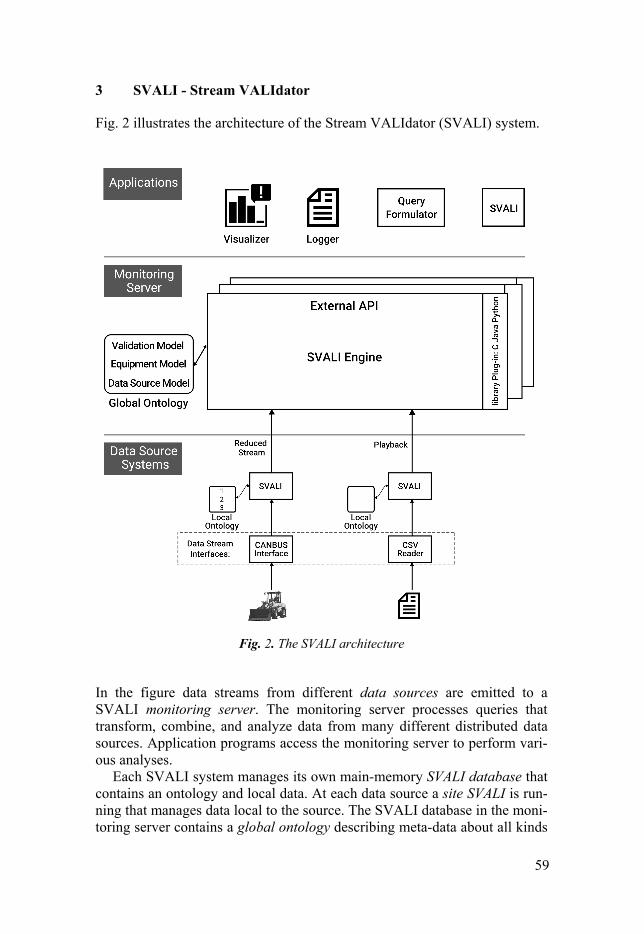
59
3 SVALI - Stream VALIdator
Fig. 2 illustrates the architecture of the Stream VALIdator (SVALI) system.
Fig. 2. The SVALI architecture
In the figure data streams from different data sources are emitted to a SVALI monitoring server. The monitoring server processes queries that transform, combine, and analyze data from many different distributed data sources. Application programs access the monitoring server to perform vari-ous analyses.
Each SVALI system manages its own main-memory SVALI database that contains an ontology and local data. At each data source a site SVALI is run-ning that manages data local to the source. The SVALI database in the moni-toring server contains a global ontology describing meta-data about all kinds

60
of monitored equipment, while the SVALI database at each site SVALI con-tains a local ontology describing the particular monitored equipment.
One kind of data source is data streams from wheel loaders, which are streamed to the monitoring server through a SVALI peer via a CANBUS interface. This kind of data source producing online streams is called a streaming data source. The SVALI peer encapsulates a streaming data source and a local ontology over which CQs are executed.
Another important kind of data source is CSV files containing logged data streams from monitored equipment. Data streams logged in CSV files can be played-back by SVALI and also streamed to the monitoring server.
Both local and global ontologies are organized in three levels, as illus-trated by Fig. 2. The equipment model is a common meta-data model that describes general properties common to all kinds of equipment, e.g. meta-data about sensor models and wheel loaders. The data source model maps raw data from a particular kind of data source to the common meta-data model. The validation model identifies anomalies in each kind of monitored equipment in terms of the data source and common meta-data models.
For example, the data source model of wheel loaders, the wheel loader model, maps data from raw data streams and log files into the common meta-data model. The validation model of wheel loaders includes a statistical model that identifies clutch slippages based on streams from sensors moni-tored through a CANBUS interface.
To handle computations in CQs that cannot be expressed as built-in func-tions, the SVALI engine provides an algorithm plug-in mechanism. The plug-in can be used to implement specific algorithms, like indexing, compu-tations, matching, optimization, and classification functions. Plug-ins for Python and Java engines are available so that algorithms written in these languages can be accessed by SVALI without any changes to the original code.
The applications are other systems accessing the monitoring server by sending CQs to it through the SVALI external API. The application can be, e.g., a visualizer that graphically displays data streams derived from mal-functioning equipment to indicate what is wrong, a query formulator [18] with which CQs are constructed graphically, or a stream logger that saves derived streams on disk.
3.1 The functional data model of SVALI
SVALI is built on top of the functional database management system AMOS [17] extending it with stream primitives, windowing operators, and valida-tion functionality.
The basic primitives of SVALI’s functional model are objects and func-tions. SVALI has two kinds of objects, literal and surrogate objects, where literals are immutable objects like numbers and string while surrogate ob-jects are mutable based OIDs (object IDs) managed by the system. Objects
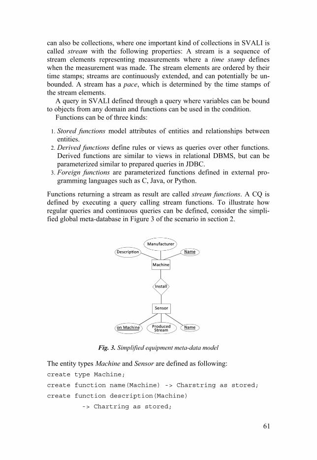
61
can also be collections, where one important kind of collections in SVALI is called stream with the following properties: A stream is a sequence of stream elements representing measurements where a time stamp defines when the measurement was made. The stream elements are ordered by their time stamps; streams are continuously extended, and can potentially be un-bounded. A stream has a pace, which is determined by the time stamps of the stream elements.
A query in SVALI defined through a query where variables can be bound to objects from any domain and functions can be used in the condition.
Functions can be of three kinds:
1. Stored functions model attributes of entities and relationships between entities.
2. Derived functions define rules or views as queries over other functions. Derived functions are similar to views in relational DBMS, but can be parameterized similar to prepared queries in JDBC.
3. Foreign functions are parameterized functions defined in external pro-gramming languages such as C, Java, or Python.
Functions returning a stream as result are called stream functions. A CQ is defined by executing a query calling stream functions. To illustrate how regular queries and continuous queries can be defined, consider the simpli-fied global meta-database in Figure 3 of the scenario in section 2.
Fig. 3. Simplified equipment meta-data model
The entity types Machine and Sensor are defined as following:
create type Machine;
create function name(Machine) -> Charstring as stored;
create function description(Machine)
-> Chartring as stored;
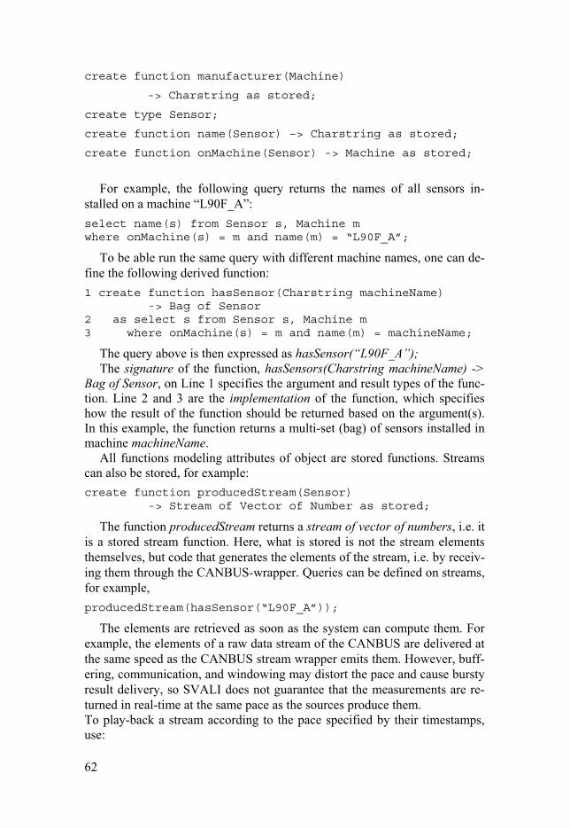
62
create function manufacturer(Machine)
-> Charstring as stored;
create type Sensor;
create function name(Sensor) –> Charstring as stored;
create function onMachine(Sensor) -> Machine as stored;
For example, the following query returns the names of all sensors in-
stalled on a machine “L90F_A”:
select name(s) from Sensor s, Machine m where onMachine(s) = m and name(m) = “L90F_A”;
To be able run the same query with different machine names, one can de-fine the following derived function:
1 create function hasSensor(Charstring machineName) -> Bag of Sensor 2 as select s from Sensor s, Machine m 3 where onMachine(s) = m and name(m) = machineName;
The query above is then expressed as hasSensor(“L90F_A”); The signature of the function, hasSensors(Charstring machineName) ->
Bag of Sensor, on Line 1 specifies the argument and result types of the func-tion. Line 2 and 3 are the implementation of the function, which specifies how the result of the function should be returned based on the argument(s). In this example, the function returns a multi-set (bag) of sensors installed in machine machineName.
All functions modeling attributes of object are stored functions. Streams can also be stored, for example:
create function producedStream(Sensor) -> Stream of Vector of Number as stored;
The function producedStream returns a stream of vector of numbers, i.e. it is a stored stream function. Here, what is stored is not the stream elements themselves, but code that generates the elements of the stream, i.e. by receiv-ing them through the CANBUS-wrapper. Queries can be defined on streams, for example,
producedStream(hasSensor(“L90F_A”));
The elements are retrieved as soon as the system can compute them. For example, the elements of a raw data stream of the CANBUS are delivered at the same speed as the CANBUS stream wrapper emits them. However, buff-ering, communication, and windowing may distort the pace and cause bursty result delivery, so SVALI does not guarantee that the measurements are re-turned in real-time at the same pace as the sources produce them. To play-back a stream according to the pace specified by their timestamps, use:

63
playback(producedStream(hasSensor(“L90F_A”)));
In this case the system uses the difference in time between the time stamps to determine when to deliver an emitted stream element to the user. It is possible to make derived functions that return streams, for example:
create function machineStream(Charstring machineName) -> Stream of Vector of Number as producedStream(hasSensor(machineName));
machineStream() is a stream function that returns a stream of vectors of numbers from a sensor installed on the named machine. The implementation function calls the derived function hasSensor() and the stored stream func-tion producedStream(). Executing machineStream(“L90F_A”) is another example of a CQ.
One important data type in SVALI is called stream windows. Stream windows are motivated by the idea that only the most recent stream elements are of interest, e.g. only the most recent 100 elements (count windows) or the steam elements during the last second (time windows). In SVALI, func-tions that take data streams as input and return streams of windows as output are called window functions. There are several window functions in SVALI that form different kinds of stream windows including the most common ones such as count windows and time windows. New kinds of windows are also supported by SVALI, e.g. predicate windows [33] and partition win-dows explained below. For example, count windows are formed by the func-tion cwindowize(Stream s, Integer size, Integer slide) -> Stream of Window, where s is the input stream, size is the number of stream element in the win-dow, and slide defines how many elements will be expired when a new win-dow is formed. The following CQ creates a stream of count windows with size 4 and slide 2.
cwindowize(siota(1, 10), 4, 2);
siota(1, 10) is a stream function that generates a stream of integers from 1 to 10.
3.2 Validation functionality
In order to detect unexpected equipment behavior, a validation model de-fines the correctness of a type of equipment as a set of validation functions, which for each validated stream from the equipment produces a validation stream describing the difference between measured and expected behavior. The validation model is stored as meta-data in the local database. Each tuple in a validation stream has the format (ts, mv, x, …) where ts is the time of the measurement, m is the measured value, and x is the expected value. In addi-tion, application dependent values describing an anomaly are included in each validation stream element. For example, a CANBUS stream contains measurements of different kinds, so the validation stream elements include
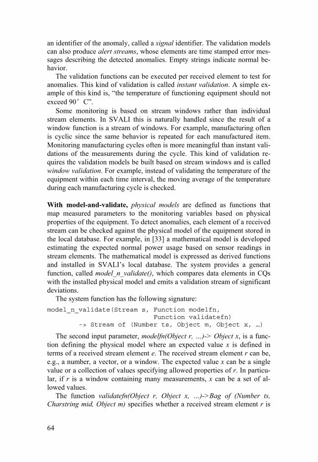
64
an identifier of the anomaly, called a signal identifier. The validation models can also produce alert streams, whose elements are time stamped error mes-sages describing the detected anomalies. Empty strings indicate normal be-havior.
The validation functions can be executed per received element to test for anomalies. This kind of validation is called instant validation. A simple ex-ample of this kind is, “the temperature of functioning equipment should not exceed 90°C”.
Some monitoring is based on stream windows rather than individual stream elements. In SVALI this is naturally handled since the result of a window function is a stream of windows. For example, manufacturing often is cyclic since the same behavior is repeated for each manufactured item. Monitoring manufacturing cycles often is more meaningful than instant vali-dations of the measurements during the cycle. This kind of validation re-quires the validation models be built based on stream windows and is called window validation. For example, instead of validating the temperature of the equipment within each time interval, the moving average of the temperature during each manufacturing cycle is checked. With model-and-validate, physical models are defined as functions that map measured parameters to the monitoring variables based on physical properties of the equipment. To detect anomalies, each element of a received stream can be checked against the physical model of the equipment stored in the local database. For example, in [33] a mathematical model is developed estimating the expected normal power usage based on sensor readings in stream elements. The mathematical model is expressed as derived functions and installed in SVALI’s local database. The system provides a general function, called model_n_validate(), which compares data elements in CQs with the installed physical model and emits a validation stream of significant deviations.
The system function has the following signature:
model_n_validate(Stream s, Function modelfn, Function validatefn) -> Stream of (Number ts, Object m, Object x, …)
The second input parameter, modelfn(Object r, …)-> Object x, is a func-tion defining the physical model where an expected value x is defined in terms of a received stream element e. The received stream element r can be, e.g., a number, a vector, or a window. The expected value x can be a single value or a collection of values specifying allowed properties of r. In particu-lar, if r is a window containing many measurements, x can be a set of al-lowed values.
The function validatefn(Object r, Object x, …)->Bag of (Number ts, Charstring mid, Object m) specifies whether a received stream element r is

65
invalid compared to the expected value x as computed by the model func-tion. In case r is invalid the validation function returns a set of pairs (ts,mid,m) representing the time of each invalid measurement m named mid detected in r.
The model function can also be a stored function populated by, e.g., min-ing historical data. In that case the reference model is first mined offline and the computed parameters explicitly stored in the stored function modelfn() passed to model_n_validate(). In this paper, the reference model of the wheel loader scenario is learnt offline and then used by the validation function, as explained below. With learn-and-validate models are defined that dynamically adapt to re-ceived stream elements, for example based on statistical models collecting data from the stream during learning phases where the behavior of the equipment is guaranteed to be correct. Such kind of model is called a learn-and-validate model. To automatically learn a model of correct equipment behavior based on observed streaming data, the system provides the built-in function learn_n_validate(). It records the actual behavior of the monitored equipment and builds a statistical model based on the sampled correct behav-iors. After the learning phase, the learnt model is used as the reference model with which the streaming data will be compared. As model-and-validate, the system emits a validation stream when significant deviations are detected.
The learn-n-validate function has the following signature:
learn_n_validate(Stream s, Function learnfn, Integer n, Function validatefn) -> Stream of (Number ts, Object m, Object e, …)
The learning function learnfn() builds the reference model on n sampled stream elements. The advantage with learn-and-validate is that the statistics is more up-to-date than with an offline model such as model-and-validate. Also it does not require defining the physical model. Offline models may be defined based on the comparing the online stream with historical data.
3.3 Extensibility
Parts of the data processing will require advanced computations such as nu-merical and statistical computations made in real-time over the data elements streaming through SVALI. The numerical computations are often provided as algorithms and packages implemented in some conventional program-ming language such as Java or C. Rather than having to re-implement the algorithms in a new language, it should be possible to call packages imple-mented in a programming language from CQs without having to change the implementations of the algorithms. To cope with this challenge, SVALI is extensible by allowing for calling (dynamically linked) application depend-ent foreign functions implemented in some conventional programming lan-
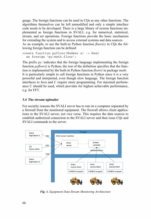
66
guage. The foreign functions can be used in CQs as any other functions. The algorithms themselves can be left unmodified and only a simple interface code needs to be developed. There is a large library of system functions im-plemented as foreign functions in SVALI, e.g. for numerical, statistical, stream, and set operations. Foreign functions provide the basic mechanism for extending the system and to access external systems and data sources. As an example, to use the built-in Python function floor(x) in CQs the fol-lowing foreign function can be defined:
create function pyfloor(Number x) -> Real as foreign 'py:math.floor';
The prefix py: indicates that the foreign language implementing the foreign function pyfloor() is Python; the rest of the definition specifies that the func-tion is implemented by the built-in Python function floor() in package math. It is particularly simple to call foreign functions in Python since it is a very powerful and interpreted, even though slow language. The foreign function interfaces to Java and C require more programming. For maximal perform-ance C should be used, which provides for highest achievable performance, e.g. for FFT.
3.4 The stream uploader
For security reasons the SVALI server has to run on a computer separated by a firewall from the monitored equipment. The firewall allows client applica-tions to the SVALI server, not vice versa. This requires the data sources to establish authorized connection to the SVALI server and then issue CQs and SVALI commands to the server.
Fig. 4. Equipment Data Stream Monitoring Architecture

67
Fig. 4 illustrates the equipment data stream monitoring architecture. On the remote sites there are embedded SVALI source clients, running on-board the wheel loaders, accessing local data streams via the CANBUS data stream wrapper. The STREAM uploader is a SVALI component that executes a local CQ which receives streaming data from the equipment. The CQ filters and transforms the data stream before emitting it to the SVALI server. To authenticate stream delivery to the SVALI server, the source client has to first issue an authentication request. After authentication the system starts on-line stream delivery to the SVALI server in real-time. The STREAM uploader logs the uploaded measurements in temporary CSV files on the server, which are simultaneously tailed by the SVALI server when one or several CQs are activated. These CSV files also provide logs of the uploaded data. The logs can either be automatically deleted by the system after some time or uploaded to regular databases for further analyzes.
The uploaded streams are analyzed by application CQs accessing them in terms of stream identifiers managed by the SVALI server. Client applica-tions can access SVALI either through a CQ query editor [18] that allows engineers to graphically specify CQs, or through client applications sending CQs to SVALI for execution.
4 Functional anomaly detection
The theory behind the validation model used for monitoring wheel loaders is based on a general statistical model to determine anomalies in streaming data, presented next.
4.1 Higher Order Cumulant
Higher-order cumulants are useful in diverse applications for many years for their ability to handle non-Gaussian processes [26]. Cumulants above the third-order are regarded as higher order cumulants while lower order cumu-lants are from the third-order and below [13].
Higher-order cumulants are preferred instead of second-order for signals corrupted with Gaussian measurement noise since they are blind to Gaussian processes [21]. Cumulants and Moments are different terms [10]. The moment of an ergodic random process is given as = = ( ) = 1,2, … [5]
where ( ) is the probability density function. Moments defined about the mean are referred to as central moments [5]. The central moment of an ergodic random process is defined as
68
= ( − ́) = ( − ́ ) ( ) = 1,2, …
where ́ is the mean and ( ) is the probability density function [5]. The first central moment is always zero, the second central moment is the variance, and the third central moment is the skewness [10][21]. The first, second and third order cumulants happens to be equal to the first, second and third central moments, but the fourth order cumulant is not equal to the fourth central moment but rather a complicated polynomial function of the central moment [10][13][26].
Cumulants higher than the fourth order result in even much more mathe-matical complications [10].
The first, second, third and fourth order cumulants are defined as [21]: , = ( ) , ( ) = ( ( ) − ( ) )( ( + ) − ( + ) ) , , = ( ( ) − ( ) )( ( + ) − ( + ) )( ( +) − ( + ) ) , ( , , ) = ( ( ) − ( ) )( ( + ) − ( + ) )( ( +) − ( + ) )( ( + ) − ( + ) )
where the th-order cumulants is a function of -1 lags [21]. , ( , , ) is a higher order cumulant [13]. Kurtosis is based on the fourth order cumulant and thus a higher order
cumulant [9].The Kurtosis is the normalized fourth order cumulant about the mean and it is given by = ( ( ) − ( ) )( ( ( ) − ( ) ) ) =
where is the fourth order cumulant and is the standard deviation [9]. The kurtosis gives an indication of the “peakedness” of a signal and the
tailedness of a probability density function. For a normal distribution the kurtosis value is 3 but − 3 = 0 is often used [9].
4.2 Implementation of Kurtosis in SVALI
The data is streamed to SVALI through in the format of vectors of numbers called frames. Each frame is a tuple with the following format:
(ts, frameid, v1, v2 , … , vi) ts is the time of the measurement. Each frame of type frameid measures a set of signals, signals(frameid)= {sig1, sig2,…,sigi}, which are stored as meta-data in SVALI. vi is the sensor reading of sigi in the frame. In the application there are five types of frames, as in Table 1.

69
Frame ID Signals 10 ForwardPressure1, ForwardPressure2, MainPres-
sure, ForwardPressure3 11 PressureR, RearTorque, FrontTorque
2364542723 InputSpeed, TurbTorque, TrmOiltem, Shift-ing1To2, OffgSlipping, OngSlipping, Gear,
DirGear 2364542467 DiffSpeed1, DiffSpeed2, TurbSpeed, OutgSpeed 15 OutputCoolerTemp
Table 1. Five types of frames
A value set vs(sig, w) is a set of values for a signal sig in a window w. In order to analyze statistics about a set of observed signals named sigi ∈ SIG in CQs, SVALI provides a function valueSets(SIG, w) that computes the values sets of the signals named oi in window w, vs(sigi,w). On the value sets different kinds of statistical aggregate functions can be applied, e.g. to de-termine anomalies in the values sets of SIG by using kurtosis.
In the application, the aggregate function kurtosis(V) computes a measure of the peakedness of the probability distribution of the values in a value set V. To determine anomalies of signals SIG detected in window w, the kurtosis of vs(sigi,w) is compared with the expected maximum kurtosis emk(sigi) for each signals sigi stored as meta-data. An anomaly is detected when kur-sosis(vs(sigi,w)) > emk(sigi) from some signal sigi measured by some frame in window w.
Partition windows. In the Volvo wheel loader scenario, one important sig-nal is the gear sensor reading which specifies the current gear of the wheel loader. All the frames read from the sensors when the current gear does not change are called one gear cycle and is defined as a partition window where a new window is started when the gear changes. In general, partition win-dows in SVALI are defined based on the value changes of one or several partition attributes of the stream elements. In the example the partition at-tribute is gear, which identifies the current gear. When partition attribute values change, the previous window is emitted and new one is started. Parti-tion windows are defined by the function partwindowize(Stream s, Function partitionBy) -> Stream of Window. The partition function partitionBy(Object o) -> Object p maps a received stream element o to p, where the value change of p is used to partition the stream s to form stream windows.
In the Volvo wheel loader scenario, the partition function defines the gear as the partition attribute, which is the 9th element in the frame.
create function gear(Vector of Number frame) -> Number g as frame[8];

70
The stream s is then partitioned into a stream of windows when the gear is changed by the function partwindowize(s, #’gear’). To detect anomalies in observed signals during each gear cycle, on each partition window the Kur-tosis of each observed signal is calculated and compared with its maximum allowed Kurtosis value. The validation over a CANBUS stream s is specified by model_n_validate(s, #’allowedKurtosis’, #’anomalies’). The model func-tion allowedKurtosis(Window pw) -> Bag of (Charstring sigi, Number ai) returns a set of pairs (sigi, ai) representing the allowed Kurtosis ai of each observed signal sigi in the partition window pw. The validation function anomalies(Window pw, Bag of (Charstring sigi, Number a) exp) -> Bag of (Number ts, Charstring sigj, Number mj) returns a set of triples (ts, sigj, mj), indicating time stamped invalid measurements mj of signal sigj in pw.
The function allowedKurtosis() is defined as:
create function allowedKurtosis(Window pw) ->Bag of (Charstring sigi, Number ai) as select sigi, maxAllowedKurtosis(sigi) from Vector of Number vs where vs = valueSet(sigi, pw);
The function maxAllowedKurtosis(Charstring sig) -> Number m is a stored function returning the allowed Kurtosis m for a signal sig.
The function anomalies() is defined as:
create function anomalies(Window pw, Bag of (Charstring sigi, Number ai) exp) -> Bag of (Number ts, Charstring sig, Number mi) as select ts(w), sigi, mi where mi = measuredKurtosis(exp) and (sigi, ai) in exp and mi > ai;
The function returns the anomalies detected in pw by selecting the unex-pected measured kurtosis values mi of signal sigi that exceeds the maximum allowed value ai. The function measuredKurtosis(sigi, pw) returns the com-puted Kurtosis for signal sigi in pw. It is defined as:
create function measuredKurtosis(Charstring sigi, Window pw) -> Number mi as kurtosis(valueSet(sigi, pw));
The function kurtosis(vs) of a value set vs is defined as:
create function kurtosis(Bag of Number vs) -> Number as cumulant4(vs) / stdv(vs)^4;
where cumulant4() computes the 4th cumulate of value set vs:
create function cumulant4(Bag of Number vs) -> Number as sum(select (e – avg(vs))^4
71
from Number e where e in vs);
A CQ that returns a stream containing invalid measurements for the wheel loader named “L90F_A” is defined as:
select model_n_validate(gearcycles,#’allowedKurtosis’, #’anomalies’) from Stream of Window gearcycles where gearcycles = partwindowize( machineStream(“wheelLoaderA”), #’partBy’);
The function partwindowize() produces a stream of windows for each gear cycle on which model_n_validate() is applied using the above model.
5 Distributed equipment monitoring
Fig. 5 shows a typical configuration of SVALI in a distributed setting where a number of wheel loaders are monitored to produce data streams transmitted to a monitoring center where they are merged. Each wheel loader runs a local SVALI system running the following CQ to produce a stream of gear cycle windows from CANBUS channel 007 uploaded to the monitoring cen-ter “M1”:
upload(partwindowize(CANstream(007), #’gear’), “M1”);
Each site has an identifier which is sent to the monitoring center and there stored in a function enumerating the monitored sites sites(Number id) -> Charstring Name. The monitoring center identifies anomalies in any moni-tored machine by merging and validating the uploaded gear cycle window streams from all the sites with the CQ:
select model_n_validate(gearCycles,#’allowedKurtosis’, #’anomalies’) from Stream of Window gearCycles where gearCycles = merge(select streamFrom(site(i)) from Integer i);
The function streamFrom(Charstring site)->Stream returns the stream uploaded from a given site. The merging is done asynchronously as new tuples arrive from the sites while local queries produce streams of gear cycle windows in parallel on each wheel loader. This is possible since SVALI systems run both in the monitoring center and on each wheel loader. The execution of local queries on each wheel loader furthermore gives local con-trol on each for each site what data to send to the monitoring center. The validation is done at the monitoring center. This is called central validation.
The local SVALI systems on each wheel loader enable parallel processing of expensive functions. In particular also the expensive model_n_validate() can be run in parallel on each wheel loader as illustrated by Fig. 6. This
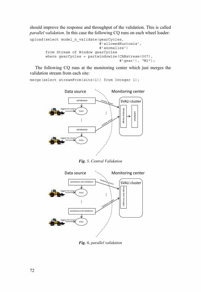
72
should improve the response and throughput of the validation. This is called parallel validation. In this case the following CQ runs on each wheel loader:
upload(select model_n_validate(gearCycles, #’allowedKurtosis’, #’anomalies’) from Stream of Window gearCycles where gearCycles = partwindowize(CANstream(007), #’gear’), “M1”);
The following CQ runs at the monitoring center which just merges the validation stream from each site:
merge(select streamFrom(site(i)) from Integer i);
Fig. 5. Central Validation
Fig. 6. parallel validation
SVALI
windowize
SVALI
windowize
...
logged CSV stream
logged CSV stream
Data source Monitoring center
SVALI cluster
...
Window
merge
validation
SVALI
windowize and validation
SVALI
windowize and validation
...
logged CSV stream
logged CSV stream
Data source Monitoring center
...
SVALI cluster
merge alert m
essages

73
6 Evaluation
The two validation strategies are experimentally evaluated to investigate the performance improvement by local SVALI validation on each site. For ex-perimental purposes, we use logged CSV files from Volvo CE wheel loaders to simulate online streams on each site. The number of validated wheel load-ers is scaled up to 100 by starting a new SVALI instances on separate nodes. The size of each recorded source data stream is around 40 MB (543917 tu-ples) having more than 500 partition windows. The result stream for validat-ing the recorded source data consists of 1054 tuples, i.e. the data reduction is about 99.81%. The experiments were made on a Dell PowerEdge R815 which has 4 CPUs with 16 2.3 GHz cores each. Both the processing capacity of SVALI and the response times (delays) were measured for different ex-perimental settings.
System Capacity
The purpose of the first experiment is to investigate the capacity of the sys-tem, i.e. how much data can be validated as the number of wheel loaders in increased. In the experiment all of the recorded data was streamed to each site SVALI at disk read speed, which is 201316 tuples/s (20 Mbytes/s per site or 5 µs/tuple), and processed by SVALI with the model above using central and parallel validation. The total throughput of processing the entire recorded streams at full speed was measured in Fig. 7. The throughput of the central validation on one core was around 3.5 Mbps. The throughput of par-allel validation reached a maximum of 110 Mbps when the number of ma-chines was more than the available number of cores, 64, since more than one SVALI instance then have to run on the same core.
Fig. 7. Full speed streaming throughput
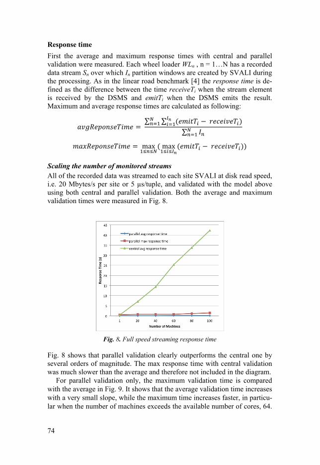
74
Response time
First the average and maximum response times with central and parallel validation were measured. Each wheel loader WLn , n = 1…N has a recorded data stream Sn over which In partition windows are created by SVALI during the processing. As in the linear road benchmark [4] the response time is de-fined as the difference between the time receiveTi when the stream element is received by the DSMS and emitTi when the DSMS emits the result. Maximum and average response times are calculated as following:
= ∑ ∑ ( − )∑ = max ( max ( − ))
Scaling the number of monitored streams All of the recorded data was streamed to each site SVALI at disk read speed, i.e. 20 Mbytes/s per site or 5 µs/tuple, and validated with the model above using both central and parallel validation. Both the average and maximum validation times were measured in Fig. 8.
Fig. 8. Full speed streaming response time
Fig. 8 shows that parallel validation clearly outperforms the central one by several orders of magnitude. The max response time with central validation was much slower than the average and therefore not included in the diagram.
For parallel validation only, the maximum validation time is compared with the average in Fig. 9. It shows that the average validation time increases with a very small slope, while the maximum time increases faster, in particu-lar when the number of machines exceeds the available number of cores, 64.

75
The figure also shows that the average times are much lower than the maxi-mum one, which means most of the validations are cheap with a few outliers.
Fig. 9. Full speed streaming parallel response time
Using actual stream rates The previous experiment was conducted with a very high data rate per site stream. In practice the stream rate is lower. We therefore measured the scal-ability of the system over the number of machines using the actual stream rates. The streams are time stamped around each 5 ms / tuple and the play-back() function was used, unlike in the first experiment.
Fig. 10 shows that in this case parallel validation also outperforms the central one. With parallel validation the average response time stays almost constant while it increases slowly when scaling the number of machines with full speed validation. However, the central validation here performs compa-rably better, as illustrated by Fig. 11 that measures the improvement ratio of central and parallel validation for the full speed and actual data rates. It shows that the response time of central validation improves a lot with the actual stream rate, which is because the playback function delays the deliv-ery of the data streams and thus gives some room for the central server to do the validation.

76
Fig. 10. Playback stream average response time
Fig. 11. Improvement ratio between full speed and actual rates

77
Scaling the site stream rates
To investigate how different site stream rates influence the validation scalability, they were scaled from 1 ms to 10 ms per tuple while keeping the number of machines constant at 100. As shown in Fig. 12 and 13, central validation gets saturated when the stream rate is high while for parallel validation both the maximum and average response times are virtually rate independent as long as there are sufficient computational resources.
Fig. 12. Validate 100 machines with different arrival rates
Fig. 13. Validate 100 machines with different arrival rates
In conclusion, we show that the parallel validation in SVALI scales very well w.r.t. response time, and system throughput when pushing expensive computations as close to the source as possible. In the experiments parallel validation has 0.09 second average response time, which is sufficient for our application. Different from hard real-time systems, for equipment anomaly

78
detection the average response time is much more important than the maxi-mum as long as the overall stream process can keep up with the stream rate.
7 Related work
In the last decades, data stream processing has gained a lot of research inter-ests. Several Data Stream Management Systems (DSMSs) such as Aurora [1], STREAM [24], have been developed based on modified relational data models where variables in queries are bound to rows. By contrast, SVALI uses a functional data model to express CQs where streams are first class objects in domain calculus queries. Further-more, SVALI furthermore al-lows calling external libraries as foreign functions so that complex algo-rithms over data streams can be efficiently implemented and used in CQs.
Various research issues on outlier detection for data streams are discussed in [29]. In our work, unexpected behavior of the equipment can also be seen as outlier from normal behavior. Because data streams are online and dy-namic, outlier detection in the stream context becomes fundamentally differ-ent than regular outlier detections, which often done in a store-and-process fashion. In [29] previous work on stream outlier detection is categorized into four major categories: (i) outlier detection over sliding windows [3][8][31] [35], (ii) auto-regression [22] , (iii) data stream clustering [35], and (iv) sta-tistical density functions over data stream elements [14][31][37]. Because SVALI makes no difference between regular data types and stream objects, anomaly detection using SVALI’s built in validation functions falls into the first category. Our application, validating correct behavior of wheel loaders with a Kurtosis-based statistical model is used, shows that the domain query language of SVALI provides a powerful tool to express statistical and other numerical functions in mathematical models that identify abnormal behavior of the equipment. Hence, our work also belongs to the fourth category.
There are two main parallelization strategies for processing data streams. One is to parallelize the continuous query execution plans [2][16], where operators are placed on different compute nodes. The other is to partition the input streams into sub-streams, on which CQs are applied [7][36] in parallel. In SVALI, the latter strategy is used by parallelizing expensive validations over the equipment sites. The very high reduction in streams data rates for anomaly detection makes parallel validation particularly favorable.
In [34], the authors describe an approach resembling our Kurtosis model for fault detection in locomotives as an add-on to the CBR diagnosis system [32]. Like in our system, the signals are processed individually to detect an anomaly and then fused together using another machine learning algorithm. They use a non-parametric test to detect individual anomalies and a general-ized regression neural network to combine the signals to one anomaly indi-cation output. However, they do not describe how they integrate the CBR system and the anomaly detection part, while we show how the functional

79
data model of SVALI enables convenient integrated of data streams from distributed equipment.
In other work on anomaly detection from equipment, e.g. by Tatsuhito et al [23] Mäki et al [20], Marklund et al [19], Katsuhiro et al [15], Fatima et al [11], Kazunari et al [25], Berglund [6], the anomaly detection is made in test-rigs, but not in the actual heavy duty machines. In our application clutch slippage detection and diagnoses are done on-board the equipment where streams of sensors are processed on the machine by an extensible on-board DSMS system using a CAN bus wrapper. The DSMS enables the anomaly detection to be expressed on a very high level as CQs using a functional anomaly detection model.
8 Conclusions and future work
We presented a general system, SVALI, to detect anomalies in data streams. Anomalies in the behavior of heavy duty equipment stream are detected by running SVALI on-board the machines. In SVALI anomaly detection rules are expressed declaratively as continuous queries over mathemati-cal/statistical models that match incoming streamed sensor readings against an on-board database of normal readings.
To enable scalable validation of geographically distributed equipment, SVALI is a distributed system where many SVALI instances can be started and run in parallel on the equipment. Central analyses are made in a moni-toring center where streams of detected anomalies are combined and ana-lyzed.
The functional data model of SVALI provides definition of meta-data and validations models in terms of typed functions. Continuous queries are ex-pressed declaratively in terms of a domain calculus where streams are first class objects. Furthermore, SVALI is an extensible system where functions can be implemented using external libraries written in C, Java, and Python without any modifications of the original code.
To control the transmission of equipment data streams to the monitoring center, there is a firewall around the monitoring center. Therefore, the data streams from the equipment are transmitted to the monitoring center using a stream uploader, rather than accessing the sensored data in the inverse direc-tion from the monitoring center.
To enable stream validation on a high level, the system provides two sys-tem validation functions, model_n_validate() and learn_n_validate(). model_n_valdiate() allows the user to define mathematical models based on physical properties of the equipment to detect unexpected equipment behav-ior. The model can also be built using historical data and then stored in the database as reference model. In the scenario from Volvo CE, the maximum allowed Kurtosis is first built off-line and then used to detect clutch slip-pages of wheel loaders. By contrast, learn_n_validate() builds statistical
80
model by sampling the stream on-line as it flows. The model can also be re-learnt in order to keep updated, e.g. after every time units or amount of stream elements.
Experimental results show that the distributed SVALI architecture enable scalable monitoring and anomaly detection with low response times when the number of monitored machines and their data stream rates increase. The experiments were made using real data recorded in running equipment. The experiments show that parallel validation where expensive computations are done in the local SVALI peers has good response time and throughput.
The monitoring capability presented is further a necessary means for monitoring large numbers, or fleets, of for instance vehicles or production equipment etc. when customers are offered result- or availability-oriented contracts. Examples of such offers are Industrial Product-Service Systems and Functional Products, where the ability to act in a proactive manner and conduct predictive maintenance based on facts are key [26].
A future work is to combine different kinds of data streams from different equipment exploring more information of the stream of the same kind to refine the model. New scalability challenges may come up w.r.t. stream joins. Another direction is to analyze parallelization strategies when there are shared computations between CQs over the same data stream.
Acknowledgement
This work is supported by EU FP7 project Smart Vortex http://www.smartvortex.eu/ and the Swedish Foundation for Strategic Re-search under contract RIT08-0041.
9 Reference
1. D. J. Abadi, D. Carney, U. Cetintemel, M. Cherniack, C. Convey, S. Lee, M. Stonebraker, N. Tatbul, and S. Zdonik: Aurora: A New Model and Architecture for Data Stream Management. The VLDB Journal 12(2), 120 - 139 (2003).
2. D. J. Abadi, Y. Ahmad, M. Balazinska, U. Cetintemel, M. Cherniack, J.-H. Hwang, W. Lindner, A. S. Maskey, A. Rasin, E. Ryvkina, N. Tatbul, Y. Xing, and S. Zdonik: The Design of the Borealis Stream Processing Engine. Proc. CIDR 2005.
3. F. Angiulli and F. Fassetti: Distance-based Outlier Queries in Data Streams: The Novel Task and Algorithms. Journal of Data Mining and Knowledge Dis-covery, 20(2), 290 - 324 (2010).
4. A. Arasu, M. Cherniack, E. Galvez, D. Maier, A. S. Maskey, E. Ryvkina, M. Stonebraker, and R. Tibbetts: Linear Road: A Stream Data Management Benchmark. Proc. VLDB 2004.
81
5. J. Bendat and A. Piersol: Engineering Applications of Correlation and Spectral. 1980.
6. K. Berglund: Predicting Wet Clutch Service Life Performance. PhD thesis, 2013.
7. L. Brenna, J. Gehrke, M. Hong, and D. Johansen: Distributed Event Stream Processing with Non-deterministic Finite Automata. Proc. DEBS 2009.
8. L. Cao, Q. Wang, and E. A. Rundensteiner: Interactive Outlier Exploration in Big Data Streams. Proc. VLDB 2014.
9. L. T. Decarlo: On the Meaning and Use of Kurtosis. Psychological Methods, pp. 292 - 307, 1997.
10. V. R. Yadolah Dodge: The Complications of the Fourth Central Moment. The American Statistician, vol. 53, no. 3, pp. 267 - 269, 1999.
11. M. P. Fatima, N. and R. Larsson: Water Contamination Effect in Wet Clutch System. 2012.
12. CANBUS. http://en.wikipedia.org/wiki/CAN_bus. 13. CUMULANT. http://en.wikipedia.org/wiki/Cumulant. 14. J. Huang, B. Zhou, Q. Wu, X. Wang, and Y. Jia: Contextual Correlation Based
Thread Detection in Short Text Message Streams: J. Intell. Inf. Syst., vol. 38, pp. 449 - 464, Apr. 2012.
15. K. Ito, M. Barker, K. Kubota, and S. Yoshida: Designing Paper Type Wet Fric-tion Material for High Strength and Durability. Proc. SAE 2012.
16. N. Jain, L. Amini, H. Andrade, R. King, Y. Park, P. Selo, and C. Venkatramani: Design, Implementation, and Evaluation of the Linear Road Benchmark on the Stream Processing Core. Proc. SIGMOD 2006.
17. T. Katchaounov, V. Josifovski, and T. Risch: Scalable View Expansion in a Peer Mediator System. Proc. DASFAA 2003.
18. E. Bauleo, S. Carnevale, T. Catarci, S. Kimani, M. Leva, and M. Mecella: De-sign, Realization and User Evaluation of the Smart Vortex Visual Query System for Accessing Data Streams in Industrial Engineering Applications. Journal of Visual Languages and Computing, vol. 25, no. 5, pp. 577 - 601, 2014.
19. P. Marklund: Permeability Measurements of Sintered and Paper Based Friction Materials for Wet Clutches and brakes. Journal of SAE International Journal of Fuels and Lubricants, vol. 3, no. 3, pp. 857 – 864, 2010.
20. R. Maki: Wet Clutch Tribology: Friction Characteristics in All-Wheel Drive Differentials. Licentiate Thesis, 2003.
21. J. Mendel: Tutorial on Higher-order Statistics (spectra) in Signal Processing and System Theory: Theoretical Results and some Applications. Proc. IEEE 1991.
22. M. Shuai, K. Xie, G. Chen, X. Ma, and G. Song: A Kalman Filter Based Ap-proach for Outlier Detection in Sensor Networks. Computer Science and Soft-ware Engineering, vol. 4, pp. 154 - 157, Dec 2008.
23. T. Miura, N. Sekine, T. Azegami, Y. Murakami, K. Itonaga, and H. Hasegawa: Study on the Dynamic Property of a Paper-based Wet Clutch. In SAE Interna-tional Congress and Exposition, 1998.
82
24. R. Motwani, J. Widom, A. Arasu, B. Babcock, S. Babu, M. Datar, G. Manku, C. Olston, J. Rosenstein, and R. Varma: Query Processing, Resource Management, and Approximation in a Data Stream Management System. Technical Report 2002-41, Stanford InfoLab, 2002.
25. K. Okabe: Proposal of Field Life Design Method for Wet Multiple Plate Clutches of Automatic Transmission on Forklift-trucks. Society of Automotive Engineers, 2009.
26. T. Olsson, E. Kallstrom, D. Gillblad, P. Funk, J. Lindstrom, L. Hakansson, J. Lundin, M. Svensson, and J. Larsson: Fault Diagnosis of Heavy Duty Ma-chines: Automatic Transmission Clutches. Workshop on Synergies between CBR and Data Mining at 22nd International Conference on Case-Based Reason-ing, September 2014.
27. A. P. Ompusunggu, J. M. Papy, S. Vandenplas, P. Sas, and H. V. Brussel: A Novel Monitoring Method of Wet Friction Clutches Based on the Post-lockup Torsional Vibration Signal. Mechanical Systems and Signal Processing, vol. 35, no. 12, pp. 345 - 368, 2013.
28. R. Maki: Wet Clutch Tribology Friction Characteristics in Limited Slip Differ-entials. PhD thesis, 2003.
29. S. Sadik and L. Gruenwald: Research Issues in Outlier Detection for Data Streams. Proc. SIGKDD 2014.
30. S. Namburu, M. Wilcutts, S. Chigusa, L. Qiao, K. Choi, and K. Pattipati: Sys-tematic Data-driven Approach to Real-time Fault Detection and Diagnosis in Automotive Engines. IEEE Autotestcon, pp. 59 - 65, Sept 2006.
31. S. Subramaniam, T. Palpanas, D. Papadopoulos, V. Kalogeraki, and D. Gun-opulos: Online Outlier Detection in Sensor Data using Non-parametric Models. Proc. VLDB 2006.
32. A. Varma and N. Roddy: ICARUS: Design and Deployment of a Case-based Reasoning System for Locomotive Diagnostics. Engineering Applications of Artificial Intelligence, vol. 12, no. 6, pp. 681 - 690, 1999.
33. C. Xu, D. Wedlund, M. Helgoson, and T. Risch: Model-based Validation of Streaming Data (industry article). Proc. DEBS 2013.
34. F. Xue, W. Yan, N. Roddy, and A. Varma: Operational Data Based Anomaly Detection for Locomotive Diagnostics. MLMTA, pp. 236 - 241, CSREA Press, 2006.
35. D. Yang, E. A. Rundensteiner, and M. O. Ward: Neighbor-based Pattern Detec-tion for Windows over Streaming Data. Proc. EDBT 2009.
36. E. Zeitler and T. Risch: Massive Scale-out of Expensive Continuous Queries. Proc. VLDB 2011.
37. J. Zhang, Q. Gao, and H. Wang: Spot: A system for Detecting Projected Out-liers from High Dimensional Data Streams. Proc. ICDE 2008.

Paper II

85
Grand Challenge: Implementation by Frequently Emitting Parallel Windows and User-Defined Aggregate Functions Sobhan Badiozamany
Uppsala University Sweden
Cheng Xu
Uppsala University
Sweden
Tore Risch
Uppsala University
Sweden
Thanh Truong
Uppsala University Sweden
Lars Melander Uppsala University
Sweden
Emails: [email protected]
ABSTRACT
Our implementation of the DEBS 2013 Challenge is based on a scalable, parallel, and extensible DSMS, which is capable of processing general con-tinuous queries over high volume data streams with low delays. A mecha-nism to provide user defined incremental aggregate functions over sliding windows of data streams provide real-time processing by emitting results continuously with low delays. To further eliminate delays caused by time critical operations, the system is extensible so that functions can be easily written in some external programming language. The query language pro-vides user defined parallelization primitives where the user can express que-ries specifying how high volume data streams are split and reduced into lower volume parallel data streams. This enables expensive queries over data streams to be executed in parallel based on application knowledge. Our OS-independent implementation was tested on several computers and achieves the real-time requirement of the challenge on a regular PC.
Categories and Subject Descriptors
H.2.4 [Database Management]: Systems – Parallel databases, Query proc-essing
Keywords
Parallel data stream processing; continuous queries; spatio-temporal window operators.
86
1 INTRODUCTION
Monitoring a soccer game requires a system than can process, in real-time, large volumes of data to dynamically determine physical properties as they appear. This requires a system having the following properties:
• To keep up with the very high data flow the system must deliver high throughput while processing expensive computations over high volume data.
• Response in real-time requires continuous delivery of query results with low latency.
• Continuous identification of physical phenomena, such as moving balls and players, requires complex spatio-temporal algebraic com-putations over windows.
Our EPIC (Extensible, Parallel, Incremental, and Continuous) DSMS pro-vides very high throughput and low latency through parallelization, extensi-bility, and user defined incremental aggregation of windowed data streams. The high level query language provides numerical data representations and data stream windows as first class objects, which simplifies complex nu-merical computations over streaming data and enables automatic query op-timization. To provide very high performance of low level numerical and byte processing functions the system is easily extensible with user defined functions over streams and numerical data, which allows accessing external systems and plugging in time-critical user algorithms.
EPIC extends the SCSQ system [9] with several kinds of data stream windows and incremental evaluation of user-defined aggregate functions over the windows. In particular the window operator FEW (Frequently Emit-ting Windowizer) decouples the frequency of emitted tuples from a win-dow’s slide.
To process expensive queries with high-throughput and low latency the system provides application specific stream parallelization functions where general distribution queries specify how to parallelize and reduce outgoing data streams.
2 THE EPIC APPROACH
First FEW and its incremental user-define aggregation are presented in sec-tions 2.1 and 2.2, and then the solution is outlined in section 2.3.
Figure 1 shows the overall data stream flow of the implementation. The thickness of the arrows in all data flow diagrams in this paper correspond to the relative volume of the data streams. Each node in the dataflow diagram is a separate OS process, called a query processing node, in which a partial continuous execution plan is running. The topology of the dataflow diagram is completely expressed in the query language where it is possible to specify
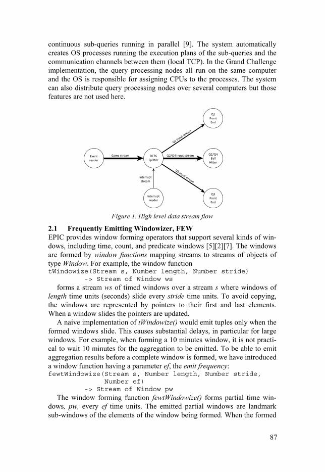
87
continuous sub-queries running in parallel [9]. The system automatically creates OS processes running the execution plans of the sub-queries and the communication channels between them (local TCP). In the Grand Challenge implementation, the query processing nodes all run on the same computer and the OS is responsible for assigning CPUs to the processes. The system can also distribute query processing nodes over several computers but those features are not used here.
Figure 1. High level data stream flow
2.1 Frequently Emitting Windowizer, FEW EPIC provides window forming operators that support several kinds of win-dows, including time, count, and predicate windows [5][2][7]. The windows are formed by window functions mapping streams to streams of objects of type Window. For example, the window function tWindowize(Stream s, Number length, Number stride) -> Stream of Window ws
forms a stream ws of timed windows over a stream s where windows of length time units (seconds) slide every stride time units. To avoid copying, the windows are represented by pointers to their first and last elements. When a window slides the pointers are updated.
A naive implementation of tWindowize() would emit tuples only when the formed windows slide. This causes substantial delays, in particular for large windows. For example, when forming a 10 minutes window, it is not practi-cal to wait 10 minutes for the aggregation to be emitted. To be able to emit aggregation results before a complete window is formed, we have introduced a window function having a parameter ef, the emit frequency: fewtWindowize(Stream s, Number length, Number stride, Number ef) -> Stream of Window pw
The window forming function fewtWindowize() forms partial time win-dows, pw, every ef time units. The emitted partial windows are landmark sub-windows of the elements of the window being formed. When the formed
88
window is complete it is emitted as well before it slides, and then the land-mark is reset to the start time of the newly slided window.
The FEW windows are required when: The results must be emitted before the window is formed. The results must be emitted more often than the slide (not used in
this application).
2.2 User-defined incremental window aggregate functions
The windowing mechanism in EPIC supports incrementally evaluated user defined aggregate functions [1][8]. These are defined by associating init(), add(), and remove() functions with a user defined aggregate function:
init() -> Object o_new creates a new aggregation object, o_new,
which is used for accumulating changes in a window. add(Object o_cur, Object e) -> Object o_nxt takes the current ag-
gregation object o_cur and the current stream element e and returns the updated aggregation object o_nxt.
remove(Object o_cur, Object e_exp) -> Object o_nxt removes from the current aggregation object o_cur the contribution of an element e_exp that has expired from a window. It returns the updated o_nxt.
A user defined aggregate function is registered with the system function: aggregate_function(Charstring agg_name, Charstring initfn, Charstring addfn, Charstring removefn) -> Object
For example, the following shows how to define the aggregate function mysum() over windows of numbers: create function initsum() -> Number s as 0; create function addsum(Number s_cur, Number e) -> Number s_nxt as res + e; create function removesum(Number s_cur, Number e_exp) -> Number s_nxt as s_cur – e_exp;
These functions are registered to the system as the aggregate function my-sum() by the function call: aggregate_function(‘mysum’,’initsum’,’addsum’,’removesum’);
After the registration mysum() can be used in CQs as: select mysum(w) from Window w where w in fewtWindowize(s, 10, 2, 1);
In this simple example the aggregation object is a single number. It can also be arbitrary objects, including dictionaries (temporary tables) holding sets of rows, which is used in the Challenge implementation to incrementally maintain complex spatio-temporal aggregations.
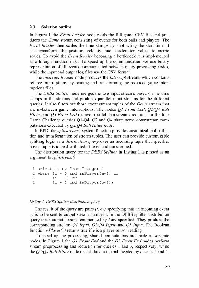
89
2.3 Solution outline
In Figure 1 the Event Reader node reads the full-game CSV file and pro-duces the Game stream consisting of events for both balls and players. The Event Reader then scales the time stamps by subtracting the start time. It also transforms the position, velocity, and acceleration values to metric scales. To avoid the Event Reader becoming a bottleneck it is implemented as a foreign function in C. To speed up the communication we use binary representation of all events communicated between query processing nodes, while the input and output log files use the CSV format.
The Interrupt Reader node produces the Interrupt stream, which contains referee interruptions, by reading and transforming the provided game inter-ruptions files.
The DEBS Splitter node merges the two input streams based on the time stamps in the streams and produces parallel input streams for the different queries. It also filters out those event stream tuples of the Game stream that are in-between game interruptions. The nodes Q1 Front End, Q2/Q4 Ball Hitter, and Q3 Front End receive parallel data streams required for the four Grand Challenge queries Q1-Q4. Q2 and Q4 share some downstream com-putations executed by Q2/Q4 Ball Hitter node.
In EPIC the splitstream() system function provides customizable distribu-tion and transformation of stream tuples. The user can provide customizable splitting logic as a distribution query over an incoming tuple that specifies how a tuple is to be distributed, filtered and transformed.
The distribution query for the DEBS Splitter in Listing 1 is passed as an argument to splitstream().
Listing 1. DEBS Splitter distribution query
The result of the query are pairs (i, ev) specifying that an incoming event ev is to be sent to output stream number i. In the DEBS splitter distribution query three output streams enumerated by i are specified. They produce the corresponding streams Q1 Input, Q2/Q4 Input, and Q3 Input. The Boolean function isPlayer(v) returns true if v is a player sensor reading.
To speed up the processing, shared computations are made in separate nodes. In Figure 1 the Q1 Front End and the Q3 Front End nodes perform stream preprocessing and reduction for queries 1 and 3, respectively, while the Q2/Q4 Ball Hitter node detects hits to the ball needed by queries 2 and 4.
1 select i, ev from Integer i 2 where (i = 0 and isPlayer(ev)) or 3 (i = 1) or 4 (i = 2 and isPlayer(ev));
90
2.3.1 Query Q1: Running Analysis
Figure 2 shows the topology of Q1. The aggregated running statistics for different time windows are computed in parallel based on the common cur-rent running statistics produced by the Q1 Front End node. The stream con-taining player sensor readings is sent to the Q1 Front End node (see Listing 1), which produces the running statistics. The running statistics is then broadcasted to four other nodes to compute the aggregated running statistics of different time window lengths.
Figure 2. Query 1 data stream flow
2.3.1.1 Incremental maintenance of running statistics
In order to make the result more reliable for the current running statistics, we first create a 1 s tumbling window and then calculate the statistics for each player over that window. The window length 1 s was chosen experimentally to produce stable results. Both running and aggregate statistics utilize user defined aggregate functions to maintain arrays of the two types of statistics for each player.
2.3.1.2 Current running statistics
For each incoming player sensor reading in the current 1 s window, the fol-lowing statistics tuple for each player is incrementally maintained in an ar-ray:
(ts_start, ts_stop, pid, left_x_start, left_y_start, left_x_stop, left_y_stop, right_x_start, right_y_start, right_y_stop, right_y_stop, sum_speed, count)
91
The time stamp ts_start stores the first time when a sensor reading of player pid arrives to the current window, while ts_stop stores the last sensor read-ing. The elements left_x_start, left_y_start, right_x_start, and right_y_start are the position readings of the left and right foot of the player at time ts_start, while left_x_stop, left_y_stop, right_x_stop, and right_y_stop are the corresponding foot position readings at time ts_stop. To incrementally calculate the average velocity the elements sum_speed and count are also included. ts_start, left_x_start, left_y_start, right_x_start, and right_y_start are updated only when the first sensor reading of the player pid arrives to the window, while all the other elements are updated every time a sensor reading of pid arrives. Here, no remove function is needed for the aggregation, since we are maintaining a stream of tumbling windows where the statistic will be re-initialized every time the window tumbles.
With the statistics above, the current running statistics for a given player is calculated as the Euclidian distance between the average position of the first and last update during the time window.
2.3.1.3 Aggregate running statistics
We have chosen to log the result tuple of Q1 in CSV format every 1 s since the current running statistics are not emitted more often than once per sec-ond. Four FEW time windows were defined for aggregating running statis-tics with lengths 1 minute, 5 minutes, 20 minutes, and the entire game. All windows slide and emit results every 1 s. FEW is critical for early emission while the first windows are being formed.
Aggregate running statistics over the window are incrementally main-tained in an array similar to current running statistics.
The stream from the Q1 Front End node contains the elements ts_start, ts_stop, player_id, intensity, distance, and speed. The difference ts_stop – ts_start is used to incrementally maintain the duration of a player being in the corresponding running intensity class. Analogously, the moving distance is maintained for the corresponding intensity classes by incrementally asso-ciating the incoming distance with the right intensity.
2.3.2 Query Q2: Ball Possession
Figure 3 shows the data flow of queries Q2 and Q4 combined. The Q2/Q4 input stream consists of player, ball, and interrupt sensor readings. The Q2/Q4 Ball Hitter computes the Ball Hitter and the Ball streams. The Ball Hitter stream contains ball hitter events, which occur when a player pid at timestamp ts hits the ball. The Ball stream contains Ball Hitter events inter-leaved with ball sensor readings. The Q2/Q4 Ball Hitter node emits the Ball stream to the Shot on Goals query processing node, which executes the final stages of query Q4. The Ball Hitter stream contains only ball hitter events
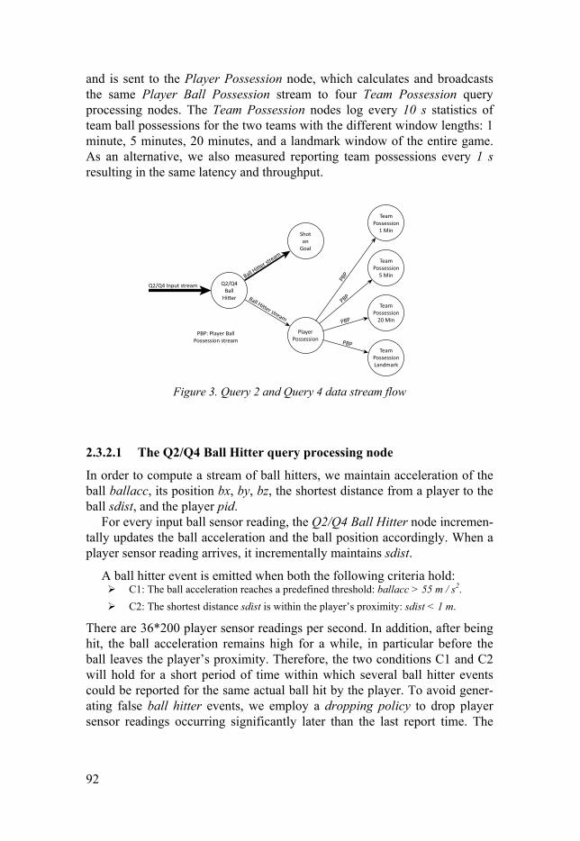
92
and is sent to the Player Possession node, which calculates and broadcasts the same Player Ball Possession stream to four Team Possession query processing nodes. The Team Possession nodes log every 10 s statistics of team ball possessions for the two teams with the different window lengths: 1 minute, 5 minutes, 20 minutes, and a landmark window of the entire game. As an alternative, we also measured reporting team possessions every 1 s resulting in the same latency and throughput.
Figure 3. Query 2 and Query 4 data stream flow
2.3.2.1 The Q2/Q4 Ball Hitter query processing node
In order to compute a stream of ball hitters, we maintain acceleration of the ball ballacc, its position bx, by, bz, the shortest distance from a player to the ball sdist, and the player pid.
For every input ball sensor reading, the Q2/Q4 Ball Hitter node incremen-tally updates the ball acceleration and the ball position accordingly. When a player sensor reading arrives, it incrementally maintains sdist.
A ball hitter event is emitted when both the following criteria hold: C1: The ball acceleration reaches a predefined threshold: ballacc > 55 m / s2.
C2: The shortest distance sdist is within the player’s proximity: sdist < 1 m.
There are 36*200 player sensor readings per second. In addition, after being hit, the ball acceleration remains high for a while, in particular before the ball leaves the player’s proximity. Therefore, the two conditions C1 and C2 will hold for a short period of time within which several ball hitter events could be reported for the same actual ball hit by the player. To avoid gener-ating false ball hitter events, we employ a dropping policy to drop player sensor readings occurring significantly later than the last report time. The
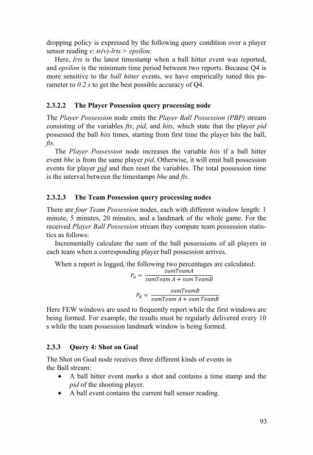
93
dropping policy is expressed by the following query condition over a player sensor reading v: ts(v)-lrts > epsilon;
Here, lrts is the latest timestamp when a ball hitter event was reported, and epsilon is the minimum time period between two reports. Because Q4 is more sensitive to the ball hitter events, we have empirically tuned this pa-rameter to 0.2 s to get the best possible accuracy of Q4.
2.3.2.2 The Player Possession query processing node
The Player Possession node emits the Player Ball Possession (PBP) stream consisting of the variables fts, pid, and hits, which state that the player pid possessed the ball hits times, starting from first time the player hits the ball, fts.
The Player Possession node increases the variable hits if a ball hitter event bhe is from the same player pid. Otherwise, it will emit ball possession events for player pid and then reset the variables. The total possession time is the interval between the timestamps bhe and fts.
2.3.2.3 The Team Possession query processing nodes
There are four Team Possession nodes, each with different window length: 1 minute, 5 minutes, 20 minutes, and a landmark of the whole game. For the received Player Ball Possession stream they compute team possession statis-tics as follows:
Incrementally calculate the sum of the ball possessions of all players in each team when a corresponding player ball possession arrives.
When a report is logged, the following two percentages are calculated: = + = +
Here FEW windows are used to frequently report while the first windows are being formed. For example, the results must be regularly delivered every 10 s while the team possession landmark window is being formed.
2.3.3 Query 4: Shot on Goal
The Shot on Goal node receives three different kinds of events in the Ball stream:
• A ball hitter event marks a shot and contains a time stamp and the pid of the shooting player.
• A ball event contains the current ball sensor reading.

94
• An interrupt event indicates a game interruption. It is good practice to reset the shot detection when an interruption occurs.
Q4 shares detection of a ball hit with Q2. However, the logic for detecting a shot is slightly different for the two queries: Q2 is specified stricter than needed for Q4. To share computations this stricter logic is also used for Q4.
The operation of Q4 is straightforward; it is iteration over the Ball stream to keep track of the state of a shot:
1 Wait for the next ball hitter event. 2 Check ball events until the ball has travelled one meter. 3 Return ball events as long as the ball is approaching the opposite
team’s goal.
The calculation of the ball direction uses basic linear algebra over the ball sensor readings.
Gravity is accounted for to an extent. The expected time for the ball to travel to the goal line is multiplied twice with the acceleration constant g, and added to the height of the goal bar. The actual ball trajectory is not con-sidered, but the current calculation should be an adequate approximation.
Using the Q2 requirements for detecting a ball hit has the drawback that some events are not detected, such as the header at 12:19 in the second half our example Game stream, since the ball is more than one meter away from any sensor. Whether that is technically a “shot” is questionable.
Curve balls need special attention. For example, at 26:07 in the first half there is a curve ball goal. In this case the direction of the ball is pointing outside the goal posts, while the ball later curves inwards and comes to rest inside the goal.
To handle curve balls we have introduced a state pending, indicating that a shot is not yet dismissed, but could later become a shot on goal. The model adds two meters of margin on both sides of the goal posts and the shot is considered pending if it points in the direction of the margin area.
Bounces are considered as long as the direction of the bounce is within the negative distance of the goal bar plus gravity. While the instructions do not account for bounces at all, this limit should add some correctness to the algebra.
Shots that are bounces, which we detect, are not included in the provided list of shots on goal. In the second half of the game there are four shots on goal that are bounces. They are at 4:11, 19:39, 24:36 and 29:29. Setting the bounce threshold to zero, i.e. not considering bounces creates a result in accordance to the specification. Viewing the video makes it apparent that the specification is not correct in this regard.
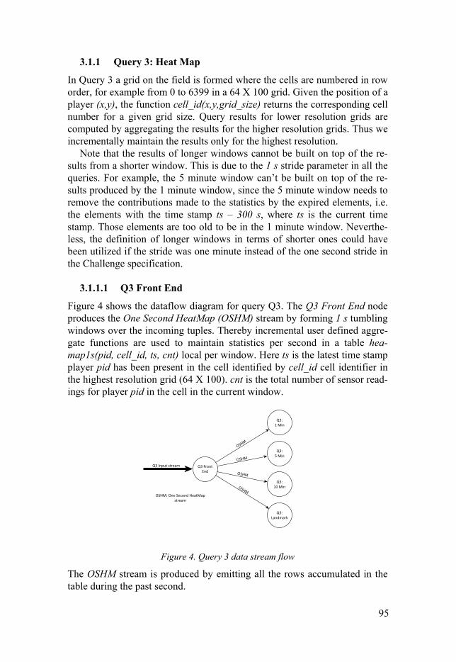
95
3.1.1 Query 3: Heat Map
In Query 3 a grid on the field is formed where the cells are numbered in row order, for example from 0 to 6399 in a 64 X 100 grid. Given the position of a player (x,y), the function cell_id(x,y,grid_size) returns the corresponding cell number for a given grid size. Query results for lower resolution grids are computed by aggregating the results for the higher resolution grids. Thus we incrementally maintain the results only for the highest resolution.
Note that the results of longer windows cannot be built on top of the re-sults from a shorter window. This is due to the 1 s stride parameter in all the queries. For example, the 5 minute window can’t be built on top of the re-sults produced by the 1 minute window, since the 5 minute window needs to remove the contributions made to the statistics by the expired elements, i.e. the elements with the time stamp ts – 300 s, where ts is the current time stamp. Those elements are too old to be in the 1 minute window. Neverthe-less, the definition of longer windows in terms of shorter ones could have been utilized if the stride was one minute instead of the one second stride in the Challenge specification.
3.1.1.1 Q3 Front End
Figure 4 shows the dataflow diagram for query Q3. The Q3 Front End node produces the One Second HeatMap (OSHM) stream by forming 1 s tumbling windows over the incoming tuples. Thereby incremental user defined aggre-gate functions are used to maintain statistics per second in a table hea-map1s(pid, cell_id, ts, cnt) local per window. Here ts is the latest time stamp player pid has been present in the cell identified by cell_id cell identifier in the highest resolution grid (64 X 100). cnt is the total number of sensor read-ings for player pid in the cell in the current window.
Figure 4. Query 3 data stream flow
The OSHM stream is produced by emitting all the rows accumulated in the table during the past second.

96
The Q3 Front End significantly reduces the stream volume by summariz-ing it. It receives 200 tuples per second from 36 sensors, in total 7200 tu-ples/second. It emits at maximum the total number of cells all the players have been present in the highest grid resolution during one second, which is about 70 tuples per second, i.e. a factor 10 reductions in stream flow.
3.1.1.2 Q3 query nodes
The OSHM stream is broadcasted to four Q3 query nodes Q3 1 Min, Q3 5 Min, Q3 10 Min, and Q3 Landmark. These nodes run parallel CQs over time windows with lengths 1, 5, 10 minutes, and whole game, respectively. The windows are formed by the FEW window specification fewtWin-dowize(oshm, length, 1, 1), where length is 60s, 300s, 600s and the whole game duration, respectively. The stride and the emit frequency are both 1 s. The emit frequency is needed so that sub-windows are emitted while the window is being formed the first time.
Similar to Q3 Front End, the Q3 query nodes incrementally maintain user defined aggregates by updating the following local tables inside each win-dow as the input stream elements arrive: heatmap(pid, cell_id, ts, cnt) sensor_count(pid, total_cnt)
In table heatmap, the attribute cell_id is the cell player pid has been pre-sent in, ts is the latest time player pid was in the cell, cnt is the number of times the player has been present in the cell. To enable translation of cnt into percentages per cell, the Q3 query nodes also maintain total_cnt per player, which stores the total number of position reports in all cells for a given player during the window in question.
Since Q3 query nodes only maintain the statistics for the highest resolu-tion in a given window length, at reporting time they compute lower resolu-tions by aggregating grid cells per player to fill the bigger cells in the higher resolutions.
The Q3 query nodes log the output CSV streams to files. Since each Q3 query nodes cover all grid settings in a given window size, the produced log files contains output stream elements for more than one grid setting. We use the following grid identifiers to tag streams per grid: 6400 for 64 X 100, 1600 for 32 X 50, 400 for 16*25, and 104 for 8 X 13 grid setting.
The size of these log files is huge (ca 400,000 rows/s) since they cover all movements between grid cells over several very long windows. Here it be-comes important to use SSD as storage medium, which is fast at writing big blocks in parallel, while disk arm movements for writing different log files has been observed to slow down the entire system throughput with a factor of around two.

97
4 PERFORMANCE
The performance of our implementation is measured based on both through-put and delay. The throughput was measured as the total execution time per query and for all queries in parallel over the entire game. The latency was measured by propagating the system wall clock of the entry time of the latest event contributing to each result tuple. The delay was calculated by subtract-ing the propagated entry time from the wall time when a result tuple is deliv-ered. The throughput is measured per query while the latency is measured per output stream.
The experiments are run on a VMware virtual machine with Windows Server 2008 R2 x64, running on a laptop with the following specifications: Dell Latitude E6530, CPU: Intel Core i7-3720QM @2.60 GHz, RAM: 8 GB, Hard Disk Device: ST500LX003-1AC15G, OS: Windows 7 64-bit.
Figure 5 illustrates the throughput of the individual queries as well as all queries running together. Queries Q1, Q2, and Q4 take around 5 minutes to finish separately, while Q3 takes considerably longer time, which is mainly due to intensive report computations in the Q3 query nodes. To investigate the log writing time, Q3 and the all queries columns have a watermark indi-cating how much time it takes to execute them without logging to disk, showing that this takes around 35 % of the Q3 alone time and 25 % of all queries together. We also investigated whether it would be favorable to par-allelize the logging of the result stream for Q3 query nodes, but that turned out to be slower in our current environment.
Figure 5. Performance
Since all queries run in parallel according to the dataflow diagrams, running all of them together takes approximately the same time as running the slow-est one, Q3.
Figure 6 shows the average delay per output stream while running all que-ries together. Notice that Q2 and Q4 are time critical queries since they im-
98
mediately report real-time phenomena. By contrast Q1 and Q3 report de-layed statistics aggregated over time.
The VMware virtual machine containing our implementation of the Grand Challenge can be downloaded from http://udbl2.it.uu.se/DEBS/. There is also a zip archive that can be run on any Windows machine.
Figure 6. Delays
5 RELATED WORK
In the stream processing community, there has been a lot of work for devel-oping query languages over data streams [5]. [7] introduced a formal specifi-cation of different kinds of windows over data streams and provided a tax-onomy of window variants. The notation of report (emit) frequency was proposed in SECRET [2] without any actual implementation. SECRET is a descriptive model to help users understand the result of window-based que-ries from different stream processing engines. Esper [4] also allows a report frequency but does not have user defined window aggregate functions. Fur-thermore Esper’s sliding window model is different from FEW because the slides are triggered by window content changes rather than explicitly speci-fied time periods.
To efficiently calculate the aggregate result over long windows with small strides, [6] and [1] use delta computations to reduce the latency and the memory usage. The focus of [8] is to extend a DSMS with online data min-ing facilities by user defined aggregate functions over windows. The imple-mentation described in this paper shows that EPIC is general enough to de-fine very complicated user defined aggregations as functions while in [1] and [8] the aggregates are defined as updates.
99
6 CONCLUSIONS We have addressed the Grand Challenge by expressing continuous queries in a high level language that supports incremental evaluation of aggregate func-tions over windows and frequently emitting windowing. We meet the real-time requirements of the real-time queries on a virtual machine running on a laptop. The extensibility of the query engine was used for supporting high throughput and low latency of time critical operations.
ACKNOWLEGEMENTS
This work was supported by the Swedish Foundation for Strategic Research, grant RIT08-0041 and by the EU FP7 project Smart Vortex.
REFERENCES 1. Bai, Y., Thakkar, H., Wang, H., Luo, C., and Zaniolo, C.: A Data Stream Lan-
guage and System Designed for Power and Extensibility. Proc. CIKM Conf., 2006.
2. Botan, I., Derakhshan, R., Dindar, N., Haas, L., Miller, R. J. and Tatbul, N. SE-CRET: A Model for Analysis of the Execution Semantics of Stream Processing Systems. Proc. VLDB Conf., 2010.
3. Botan, I., Fischer, P. M., Florescu, D., Kossmann, D., Kraska, T., and Ta-mosevicius, R. Extending XQuery with Window Functions. Proc. VLDB Conf., 2007.
4. http://esper.codehaus.org/
5. Law, Y-N, Wang, H., and Zaniolo, C.: Relational Languages and Data Models for Continuous Queries on Sequences and Data Streams. ACM TODS 36, 2, (May 2011).
6. Li, J., Maier, D., Tufte, K., Papadimos,V., and Tucker, P. A. Semantics and evaluation techniques for window aggregates in data streams. Proc. SIGMOD Conf., pp. 311 - 322, 2005.
7. Patroumpas, K. and Sellis, T. Window specification over data streams. Proc. EDBT Conf., 2006.
8. Thakkar, H., Mozafari, B. and Zaniolo, C.: Designing an Inductive Data Stream Management System: the Stream Mill Experience. Proc. 2nd International Work-shop on Scalable Stream Processing Systems, 2008.
9. Zeitler, E. and Risch, T.: Massive scale-out of expensive continuous queries, Proc. of the VLDB Endowment, ISSN 2150-8097, Vol. 4, No. 11, pp.1181-1188, 2011.


Paper III


103
Model based Validation of Streaming Data Cheng Xu
Department of Information Tech-nology
Uppsala University Box 337, SE-75105, Sweden
+46 18 471 7345 [email protected]
Daniel Wedlund
AB Sandvik Coromant R&D Application solutions,
Functional Products SE-811 81 Sandviken, Sweden [email protected]
Tore Risch Department of Information Tech-
nology Uppsala University Box 337, SE-75105
+46 18 471 6342 [email protected]
Martin Helgoson
AB Sandvik Coromant R&D Application solutions,
Functional Products SE-811 81 Sandviken, Sweden [email protected]
ABSTRACT
An approach is developed where functions are used in a data stream man-agement system to continuously validate data streaming from industrial equipment based on mathematical models of the expected behavior of the equipment. The models are expressed declaratively using a data stream query language. To validate and detect abnormality in data streams, a model can be defined either as an analytical model in terms of functions over sensor measurements or be based on learning a statistical model of the expected behavior of the streams during training sessions. It is shown how parallel data stream processing enables equipment validation based on expensive models while scaling the number of sensor streams without causing increas-ing delays. The paper presents two demonstrators based on industrial cases and scenarios where the approach has been implemented.
Categories and Subject Descriptors
H.2.4 [Database Management]: Systems – Parallel databases, Query proc-essing
Keywords
Equipment Monitoring; data stream management system; data stream valida-tion; parallelization; anomaly detection.
104
1 INTRODUCTION Emerging business scenarios such as provision of total care products, prod-uct service systems (PSS), industrial product-service-systems (IPS2), and functional products [3] [4] [5] [14] [15] imply needs to efficiently monitor, verify and validate the functionality of a delivered product in use. This can be done with regard to pre-defined criteria, e.g. productivity, reliability, sus-tainability, and quality. A functional product in this context means an inte-grated provision of hardware, software and services.
In case of machining several factors and dependencies have to be consid-ered, which in turn means that data (e.g. in-process data) from the machining process, information (e.g. about cutting tools), and knowledge (e.g. physical models), from several domains have to be captured, combined and analyzed in a comprehensive knowledge integration framework that includes quality assurance of data, validation of models, learning capabilities, and verifica-tion of functionality [10]. A considerable challenge is to scale up data analy-sis for handling huge amount of equipment.
In this context novel software technologies are needed to efficiently proc-ess and analyze the large data streams, in particular related to in-process activities, and to facilitate the steps towards increased automation of the related processes.
In manufacturing industry, equipment such as machine controllers and various sensors are installed. This equipment measure and generate data during the machining process, i.e. in-process. Depending on the case a huge amount of parameters (e.g. power, torque, etc.) at different sample rates (ranging from a couple of HZ to 20 kHZ) need to be processed. Processing data streams from controllers and sensors is critical for monitoring the func-tional product in use. For instance, the parameters related to the power con-sumption could help the engineers to analyze the process, compare different application strategies, monitor and maintain the hardware e.g. to get an indi-cation of the degree of tool-wear or when a tool needs to be replaced or ma-chine maintenance is required.
Often a mathematical model of the process can be developed, e.g. to cal-culate the expected power consumption and detect abnormal behavior. In other cases, when there is no such model pre-defined, a model can be learned based on observing sensor readings during training sessions. This requires a general approach to define the correct behavior of the equipment either ana-lytically or statistically.
Data Stream Management Systems (DSMSs), such as Aurora [1] and STREAM [16], process continuous queries, CQs, over data streams that filter, analyze, and transform the data streams. A simple CQ can be: “give me the sensor id and the power consumption whenever the power is greater than 100W”. However, detecting abnormal behavior in equipment often involves advanced computations based on knowledge about the machining

105
process, e.g. theoretical models of the equipment’s behavior, rather than just simple numerical comparisons in a query condition. An advanced CQ could be: “given a power consumption model computing the theoretical expected power consumption at any point in time, give me the sensor id whenever the difference between the actual power consumption and the theoretical ex-pected power on the average is greater than 10W during 1 second.”
To enable general stream validation based on mathematical models, the system called SVALI (Stream VALIdator) was developed and used in indus-trial applications. The system provides the following facilities:
Users can define and install their own analytical models inside the DSMS to validate correct behavior of the data streams. The models are expressed as side-effect free functions (formulae) over streamed data values.
For applications where no theoretical model can be easily defined, the system can also dynamically learn a model based on some existing observed correct behavior and then use that learned model for subsequent validation.
SVALI is a distributed DSMS extending SCSQ [22] with validation func-tionality. Many SVALI nodes can be started on different compute nodes. The distributed SVALI architecture enables processing of validations in parallel without causing unacceptable delays by the often expensive compu-tations, as shown in this paper.
The paper is organized as follows. In Section 2 the architecture of a SVALI node is presented. Section 3 presents two general strategies for stream validations in SVALI called model-and-validate and learn-and-validate, illustrated by real-life industrial examples. Section 4 presents re-sults from simulations on how the parallelization enables scalable processing of expensive validation functions in the applications, and Section 5 discusses related work. Finally, Section 6 summarizes and outlines future work.
2 SYSTEM ARCHITECTURE
Figure 1 shows the architecture of the SVALI system. Different kinds of data streams are collected from stream sources of sensor readings. SVALI is an extensible DSMS where new kinds of stream sources can be plugged in by defining stream wrappers. A stream wrapper is an interface that continu-ously reads a raw data stream and emits the read events to the SVALI kernel. On top of the stream wrappers, equipment specific stream models over raw data streams analyze the received stream tuples to validate that different kinds of equipment behave correctly. A stream model is a function over ei-ther individual stream tuples or over windows of stream tuples. Stream mod-els are passed as a parameter to the stream validator that applies the models to produce validation streams where deviations from correct behavior are indicated.
The main-memory local database stores meta-data about the streams such as stream models, tolerance thresholds, collected statistics, etc.
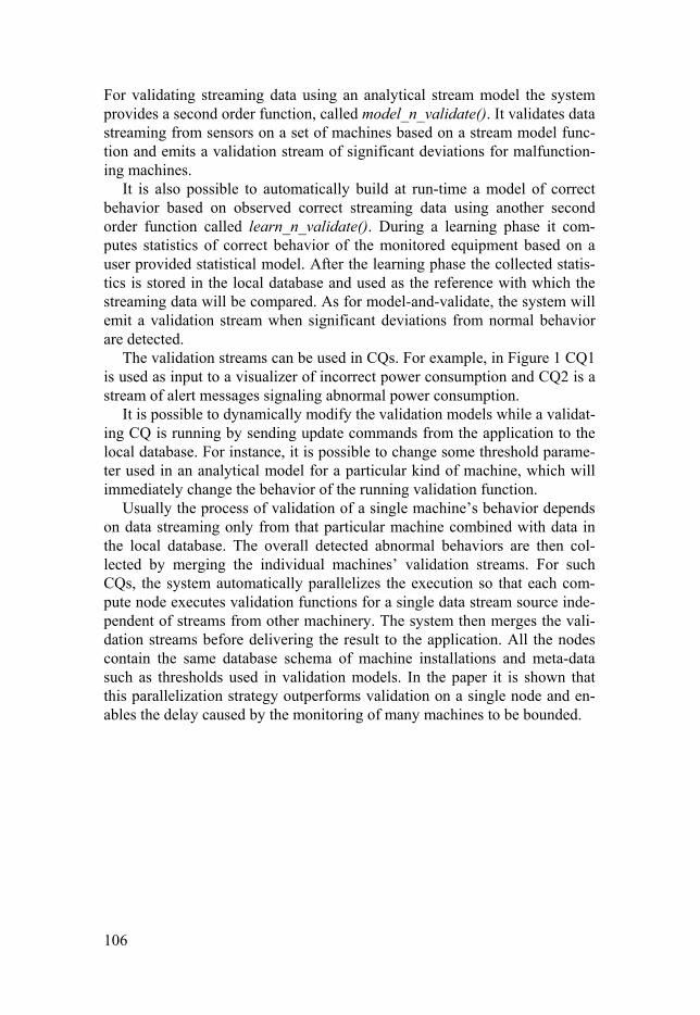
106
For validating streaming data using an analytical stream model the system provides a second order function, called model_n_validate(). It validates data streaming from sensors on a set of machines based on a stream model func-tion and emits a validation stream of significant deviations for malfunction-ing machines.
It is also possible to automatically build at run-time a model of correct behavior based on observed correct streaming data using another second order function called learn_n_validate(). During a learning phase it com-putes statistics of correct behavior of the monitored equipment based on a user provided statistical model. After the learning phase the collected statis-tics is stored in the local database and used as the reference with which the streaming data will be compared. As for model-and-validate, the system will emit a validation stream when significant deviations from normal behavior are detected.
The validation streams can be used in CQs. For example, in Figure 1 CQ1 is used as input to a visualizer of incorrect power consumption and CQ2 is a stream of alert messages signaling abnormal power consumption.
It is possible to dynamically modify the validation models while a validat-ing CQ is running by sending update commands from the application to the local database. For instance, it is possible to change some threshold parame-ter used in an analytical model for a particular kind of machine, which will immediately change the behavior of the running validation function.
Usually the process of validation of a single machine’s behavior depends on data streaming only from that particular machine combined with data in the local database. The overall detected abnormal behaviors are then col-lected by merging the individual machines’ validation streams. For such CQs, the system automatically parallelizes the execution so that each com-pute node executes validation functions for a single data stream source inde-pendent of streams from other machinery. The system then merges the vali-dation streams before delivering the result to the application. All the nodes contain the same database schema of machine installations and meta-data such as thresholds used in validation models. In the paper it is shown that this parallelization strategy outperforms validation on a single node and en-ables the delay caused by the monitoring of many machines to be bounded.

107
Figure 1. System Architecture
3 MODEL BASED VALIDATION
The functionalities of the two kinds of model based validation methods in SVALI are described along with examples of how they are applied on indus-trial equipment in use.
3.1 Model-and-validate
When the expected value can be estimated based on an analytical stream model, it is defined as a function which is passed as a parameter to the gen-eral second order function called model_n_validate() that has the following signature: model_n_validate (Bag of Stream s, Function modelfn, Function validatefn) -> Stream of (Number ts, Object m, Object x)
The user defined stream model function, modelfn(Object e)->Object x, specifies how to compute the expected value x based on a stream element e. A stream element can be a single stream tuple or a window of tuples.
The user defined validation function, validatefn(Object r, Object x)->(Number ts, Object m), specifies whether a received stream element r is invalid compared to the expected value x as computed by the model func-

108
tion. In case r is invalid the validation function returns the ts time stamped invalid measurement m in r.
The element of the validation stream returned by model-and-validate() are tuples (ts, m, x), where ts and m are computed by the validation function and x is computed by the model function.
CQs specification involving model-and-validate calls are sent to a SVALI server as a text string for dynamic execution. It is up to the SVALI server to determine how to execute the CQs in an efficient way. In particular SVALI transparently parallelizes the execution to minimize the delay caused by executing expensive validation functions.
3.1.1 Demonstrator 1
This section demonstrates how model-and-validate is used to validate the power consumption in an industrial case based on a milling scenario. The case, including the framework, meta-data, models, a cutting tool, a machine tool, related equipment to capture the needed in-process data, and a stream server called CORENET was provided by Sandvik Coromant. The streaming process data used in this demonstrator was simulated using real recorded process data from Sandvik Coromant. To be specific, the data was collected from a MoriSeiki 5000 with a Fanuc control system that was equipped with the Kistler sensor system 9255B, and DMG with a Siemens control system. The difference between running CORENET with a recorded file compared to CORENET with connection to a machine is just a matter of configuration. In this paper a consistent behavior was needed to evaluate the performance and therefore it was of benefit to use recorded data from earlier machining attempts.
Figure 2 illustrates how the milling process was performed. The parame-ters in Table 1 describe the milling process. Tool working engagement is denoted by ae feed per tooth by fz, maximum chip thickness by hex, cutting depth by ap cutting speed by vc and the number of cutting edges by zc.
Figure 2. The side milling process
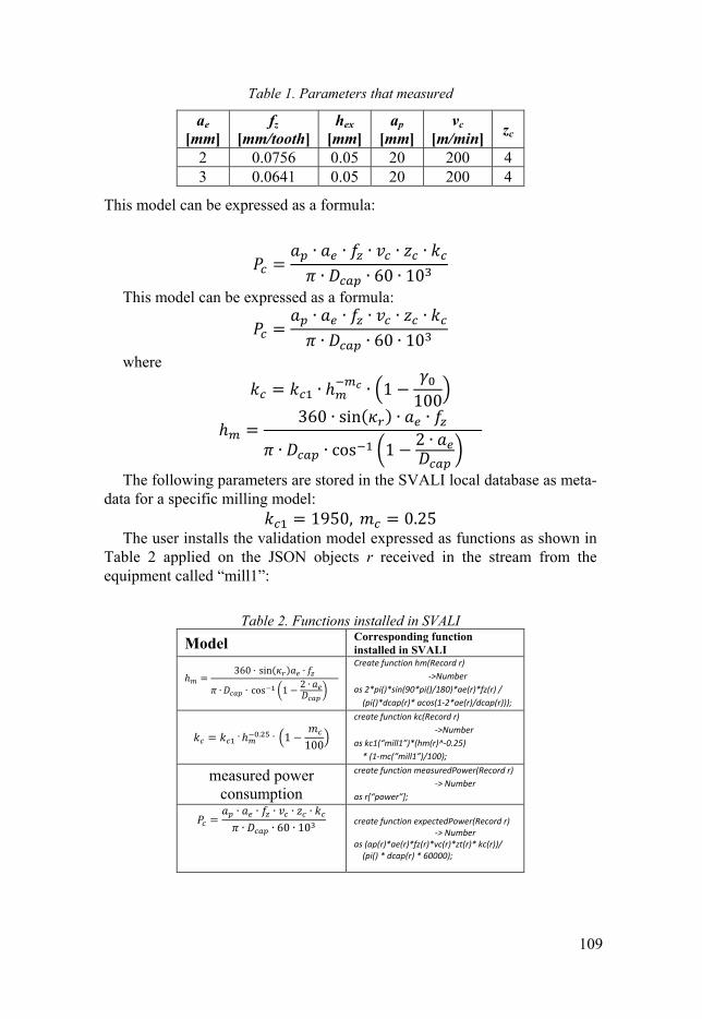
109
Table 1. Parameters that measured
ae [mm]
fz [mm/tooth]
hex [mm]
ap [mm]
vc [m/min]
zc
2 0.0756 0.05 20 200 4 3 0.0641 0.05 20 200 4
This model can be expressed as a formula:
= ∙ ∙ ∙ ∙ ∙∙ ∙ 60 ∙ 10
This model can be expressed as a formula: = ∙ ∙ ∙ ∙ ∙∙ ∙ 60 ∙ 10
where = ∙ ℎ ∙ 1 − 100 ℎ = 360 ∙ sin( ) ∙ ∙∙ ∙ cos 1 − 2 ∙
The following parameters are stored in the SVALI local database as meta-data for a specific milling model: = 1950, = 0.25
The user installs the validation model expressed as functions as shown in Table 2 applied on the JSON objects r received in the stream from the equipment called “mill1”:
Table 2. Functions installed in SVALI
Model Corresponding function installed in SVALIℎ = 360 sin( )cos 1 − 2
Create function hm(Record r) ->Number as 2*pi()*sin(90*pi()/180)*ae(r)*fz(r) / (pi()*dcap(r)* acos(1-2*ae(r)/dcap(r)));
= ℎ . 1 − 100
create function kc(Record r) ->Number as kc1(“mill1”)*(hm(r)^-0.25) * (1-mc(“mill1”)/100);
measured power consumption
create function measuredPower(Record r) -> Number as r[“power”]; = ∙ ∙ ∙ ∙ ∙∙ ∙ 60 ∙ 10
create function expectedPower(Record r) -> Number as (ap(r)*ae(r)*fz(r)*vc(r)*zt(r)* kc(r))/ (pi() * dcap(r) * 60000);
⋅ ⋅⋅ ⋅ ⋅
⋅ ⋅
110
The validation function is defined as: create function validatePower(Record r, Number x) -> (Number ts, Number m) as select ts, m where m = measuredPower(r) and abs(x - m) > th(“mill1”);
The function th(Chartsring k) is a table of validation thresholds for each kind of machine k stored in the local database. After the model is installed in the SVALI server, a CQ validating a single JSON stream delivered from host “h1” on port 1337 is expressed as: select model_n_validate(bagof(input), #'expectedPower', #’validatePower’) from Stream input where input = corenetJsonWrapper("h1", 1337);
Here, the wrapper function corenetJsonWrapper() interfaces a data stream server called “Corenet” delivering JSON objects to SVALI.
3.2 Learn-and-validate In cases where a mathematical model of the normal behavior is not easily obtained the system provides an alternative validation mechanism to learn the expected behavior by dynamically building a statistical reference model based on sampled normal behavior measured during the first n stream ele-ments in a stream. Once the reference model has been learned it is used to validate the rest of the stream. This is called learn-and-validate and is im-plemented by a stream function with the following signature: learn_n_validate(Bag of Stream s, Function learnfn, Integer n, Function validatefn) -> Stream of (Number ts, Object m, Object e)
The learning function, learnfn(Vector of Object f)->Object x, specifies how to collect statistics x, the reference model, of expected behavior, based on a sequence f of the n first streams elements.
As for model-and-validate, the validation function, validatefn(Object r, Object x)->(Number ts, Object m), returns a pair (ts, m) whenever a meas-ured value m in r is invalid at time ts compared to the reference value x re-turned by the learning function.
The function learn_n_validate() returns a validation stream of tuples (ts, m, x) with time stamp ts, measured value m, and the expected value x accord-ing to the reference model learned from the first n normally behaving stream elements.
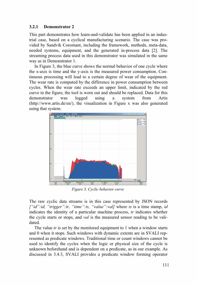
111
Figure 3. Cyclic behavior curve
3.2.1 Demonstrator 2
This part demonstrates how learn-and-validate has been applied in an indus-trial case, based on a cyclical manufacturing scenario. The case was pro-vided by Sandvik Coromant, including the framework, methods, meta-data, needed systems, equipment, and the generated in-process data [2]. The streaming process data used in this demonstrator was simulated in the same way as in Demonstrator 1.
In Figure 3, the blue curve shows the normal behavior of one cycle where the x-axis is time and the y-axis is the measured power consumption. Con-tinuous processing will lead to a certain degree of wear of the equipment. The wear rate is computed by the difference in power consumption between cycles. When the wear rate exceeds an upper limit, indicated by the red curve in the figure, the tool is worn out and should be replaced. Data for this demonstrator was logged using a system from Artis (http://www.artis.de/en/), the visualization in Figure x was also generated using that system.
The raw cyclic data streams is in this case represented by JSON records [“id”:id, “trigger”:tr, “time”:ts, “value”:val] where ts is a time stamp, id indicates the identity of a particular machine process, tr indicates whether the cycle starts or stops, and val is the measured sensor reading to be vali-dated.
The value tr is set by the monitored equipment to 1 when a window starts and 0 when it stops. Such windows with dynamic extents are in SVALI rep-resented as predicate windows. Traditional time or count windows cannot be used to identify the cycles when the logic or physical size of the cycle is unknown beforehand and is dependent on a predicate, as in our example. As discussed in 3.4.3, SVALI provides a predicate window forming operator
112
pwindowize(Stream s, Function start, Function stop)->Stream of Window that creates a stream of windows based on two predicates (Boolean func-tions) called the window start condition and the window stop condition. In this demonstrator, the start and stop condition is defined as: create function cycleStart(Record s) -> Boolean as s[“trigger”] = 1; create function cycleStop(Record s, Record r) -> Boolean as r[“trigger”] = 0 and s[“trigger”] = 1;
In our example, pwindowize() is used to build the reference model from the first two cycles of predicate windows. Analogous to the first demonstra-tor, the CQ validates a JSON stream delivered from host “h2” on port 1338 based on learn-and-validate. It is expressed as: select learn_n_validate(bagof(sw), #’learnCycle’, 2, #’validateCycle’) from Stream s, Stream sw where s= corenetJsonWrapper("h2", 1338) and sw = pwindowize(s, #’cycleStart’, #’cycleStop’);
Learning function: In our example the learning function computes the aver-age power consumption of the n first windows f in the stream. It has the definition: create function learnCycle(Vector of Window f)
-> Vector of Number
as navg(select extractPowerW(w) from Window w where w in f);
The function navg(Bag of Vector)->Vector returns the average vector of a set of numerical vectors normalized for possibly different lengths. The func-tion extractPowerW(Window w)->Vector x extracts a vector of the power consumptions of each element in window w. It has the definition: create function extractPowerW(Window w) -> Vector of Number as window2vector(w, #’extractPower’);
The function extractPower() is defined as: create function extractPower(Record r) -> Number as r[“val”];
The system function window2vector(Window w, Function fe)->Vector f creates a new vector f by applying the function fe(Object e)->Object on each element in window w.
Validation function: To validate the current stream window, we first extract the power consumption for the current window as a vector and then compare the extracted vector with the learned vector. This is defined as: create function validateCycle(Window w, Vector e) -> (Number ts, Vector of Number m)
113
as select timestamp(w), m where neuclid(e, m) > th(“machine2”) and m = extractPowerW(w);
The function neuclid(Vector x, Vector y)->Number returns the Euclidean distance between x and y normalized for different lengths.
4 PERFORMANCE EXPERIMENTS
To analyze the performance of stream validation in SVALI, the performance of model_n_validate() was measured for a set of streams with varying stream rates. Scale-up is simulated by generating many simulated streams with dif-ferent time offsets based on the raw data provided by Sandvik Coromant. The number of machines is scaled up by increasing the set of streams. The scalability of two queries was investigated:
• Q1: Given the analytical model for the power consumption of a ma-chine process above, produce a validation stream per event of those machines where the power exceeds a threshold 1.2.
• Q2: Given the analytical model for the power consumption of a ma-chine process, produce a validation stream of those machines where the power on average exceeds a threshold 1.2 for 0.1 seconds.
Query Q1 is the example query defined in Sec 3.1.1. Query Q2 uses the fol-lowing second order functions measuredPower(), expectedPower() and vali-datePower(): create function measuredPower(Window r)
-> Vector of Number m
as window2vector(r, #'measuredPower');
create function expectedPower(Window r)
-> Vector of Number x
as window2vector(r, #'expectedPower');
create function validatePower(Window r, Vector of Number x)
-> (Number ts, Vector of Number m)
as select ts(r), m
where m = measuredPower(r)
and neuclid(m, x) > th("mill1");
Given these three functions, query Q2 validating a bag of streams bsw of 0.1 second windows is defined as: model_n_validate(bsw,#’expectedPower’,#’validatePower’);
By simulation, the number of machines is scaled up to 100. Each machine emits a data stream during 30 seconds. To simulate the impact of the per-formance of streams of different stream rates, the element rate of each stream was randomly chosen between 1 and 10 ms. The validations were done both centrally and in parallel. Central validation first merges streams
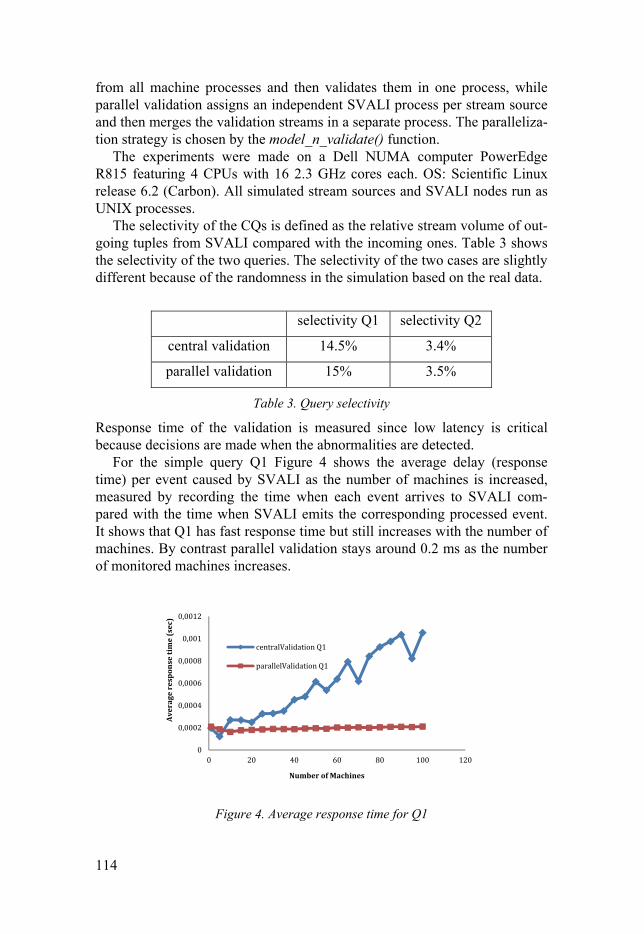
114
from all machine processes and then validates them in one process, while parallel validation assigns an independent SVALI process per stream source and then merges the validation streams in a separate process. The paralleliza-tion strategy is chosen by the model_n_validate() function.
The experiments were made on a Dell NUMA computer PowerEdge R815 featuring 4 CPUs with 16 2.3 GHz cores each. OS: Scientific Linux release 6.2 (Carbon). All simulated stream sources and SVALI nodes run as UNIX processes.
The selectivity of the CQs is defined as the relative stream volume of out-going tuples from SVALI compared with the incoming ones. Table 3 shows the selectivity of the two queries. The selectivity of the two cases are slightly different because of the randomness in the simulation based on the real data.
selectivity Q1 selectivity Q2
central validation 14.5% 3.4%
parallel validation 15% 3.5%
Table 3. Query selectivity
Response time of the validation is measured since low latency is critical because decisions are made when the abnormalities are detected.
For the simple query Q1 Figure 4 shows the average delay (response time) per event caused by SVALI as the number of machines is increased, measured by recording the time when each event arrives to SVALI com-pared with the time when SVALI emits the corresponding processed event. It shows that Q1 has fast response time but still increases with the number of machines. By contrast parallel validation stays around 0.2 ms as the number of monitored machines increases.
Figure 4. Average response time for Q1
00,00020,00040,00060,00080,0010,0012
0 20 40 60 80 100 120
Aver
age
resp
onse
tim
e (s
ec)
Number of Machines
centralValidation Q1parallelValidation Q1
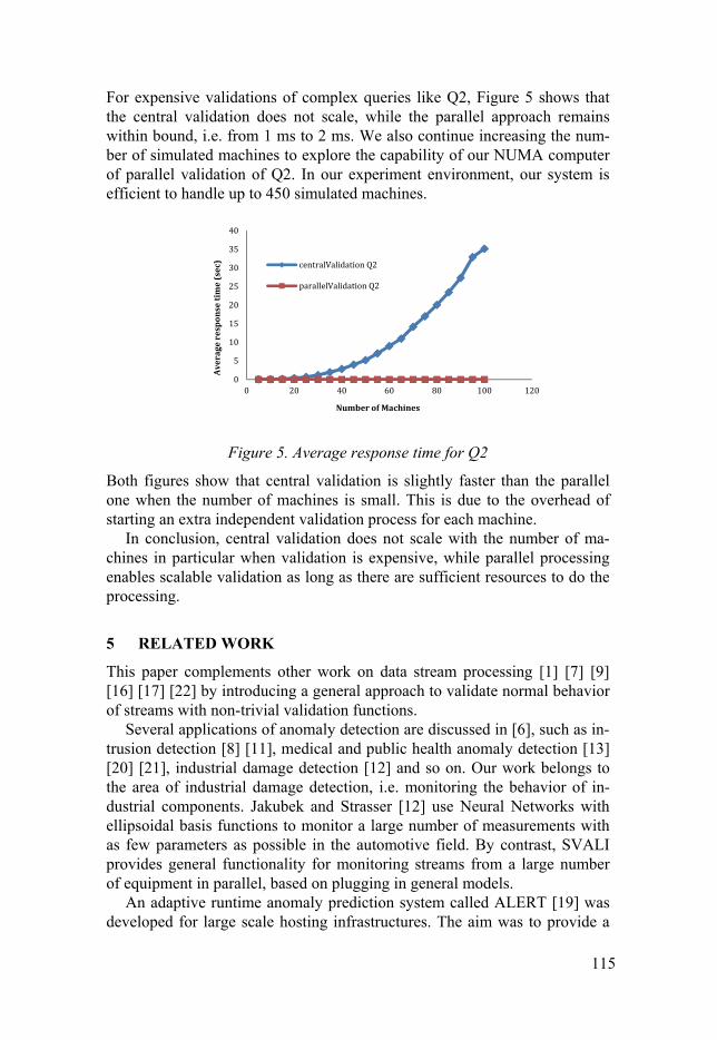
115
For expensive validations of complex queries like Q2, Figure 5 shows that the central validation does not scale, while the parallel approach remains within bound, i.e. from 1 ms to 2 ms. We also continue increasing the num-ber of simulated machines to explore the capability of our NUMA computer of parallel validation of Q2. In our experiment environment, our system is efficient to handle up to 450 simulated machines.
Figure 5. Average response time for Q2
Both figures show that central validation is slightly faster than the parallel one when the number of machines is small. This is due to the overhead of starting an extra independent validation process for each machine.
In conclusion, central validation does not scale with the number of ma-chines in particular when validation is expensive, while parallel processing enables scalable validation as long as there are sufficient resources to do the processing.
5 RELATED WORK
This paper complements other work on data stream processing [1] [7] [9] [16] [17] [22] by introducing a general approach to validate normal behavior of streams with non-trivial validation functions.
Several applications of anomaly detection are discussed in [6], such as in-trusion detection [8] [11], medical and public health anomaly detection [13] [20] [21], industrial damage detection [12] and so on. Our work belongs to the area of industrial damage detection, i.e. monitoring the behavior of in-dustrial components. Jakubek and Strasser [12] use Neural Networks with ellipsoidal basis functions to monitor a large number of measurements with as few parameters as possible in the automotive field. By contrast, SVALI provides general functionality for monitoring streams from a large number of equipment in parallel, based on plugging in general models.
An adaptive runtime anomaly prediction system called ALERT [19] was developed for large scale hosting infrastructures. The aim was to provide a
0510152025303540
0 20 40 60 80 100 120Aver
age
resp
onse
tim
e (s
ec)
Number of Machines
centralValidation Q2parallelValidation Q2

116
context aware anomaly prediction model with good prediction accuracy. Rather than anomaly prediction, we mainly focused on supporting online anomaly detection that requires more strict response time. The data streams analyzed in [19] have a fairly low arrival rate, i.e. one sample every 2 sec-onds and one sample every 10 seconds. By contrast, we show that our sys-tem can handle many streams with much higher arrival rates.
Di Wang et al. [20] proposed an active complex event processing system in a hospital environment, where rules are triggered by state changes of the system during CQ processing. In our system, validation models are stored in the SVALI local database and can be modified dynamically by update com-mands from the application side.
The main focus of [23] is time series data stream aggregate monitoring, while our approach is providing a flexible stream validation framework that can be applied on both individual event monitoring, where only latest event is of interest for processing, and aggregate monitoring, where window ag-gregation is required for the analysis. This is based on the fact that our stream validation operator treats both raw stream and windowed stream equally.
6 CONCLUSIONS AND FUTURE WORK
Two general strategies were presented to validate streams from industrial equipment, called model-and-validate and learn-and-validate, respectively. Model-and-validate is based on explicitly specifying an analytical model of expected behavior, which is compared with actual measured data stream elements. Learn-and-validate dynamically builds a statistical model based on a set of observed correct behavior in streams. We show that the approach is applicable in an industrial setting on real industrial data from real industrial machines.
In our SVALI system, continuous queries validating that equipment be-haves correctly are defined declaratively in term of validation functions that are sent to a server, which generates a parallel execution plan to enable scal-able computation of validation streams. The experiments show that parallel execution scales better than a central implementation of model-and-validate when increasing the number of streams from monitored machines.
Investigating parallelization of learn-and-validate is future work. Another interesting future work is to regularly refine the learnt model. Furthermore, the impact of complex model functions on the strategy chosen should be investigated, for instance, to validate streaming data based on trends of measured equipment behavior over time. This can be handled by defining complex model functions that compute trends over time rather than the ac-tual expected measurements. This may involve new scalability challenges.
117
ACKNOWLEGEMENTS
This work was supported by the Swedish Foundation for Strategic Research, grant RIT08-0041 and by the EU FP7 project Smart Vortex [27].
REFERENCES
10. Abadi, D.J., et al.: Aurora: a new model and architechture for data stream man-agement. The VLDB journal, 12(2), 2003.
11. Alizadeh, Z.: Method for automated tests of wear (Metod för automatisering av förslitningstest). Project work in Automated Manufacturing, 2011.
12. Alonso-Rasgado, T., Thompson, G. and Elfstrom, B.O.: The design of func-tional (total care) products. Journal of Engineering Design, Vol. 15, No. 6, pp.515-540, 2004.
13. Alonso-Rasgado, T. and Thompson, G.: A rapid design process for Total Care Product creation. Journal of Engineering Design, Vol. 17, No.6, pp.509-531, 2006.
14. Baines, T.S., Lightfoot, H.W., Evans, S., Neely, A., Greenough, R., Peppard, J., Roy, R., Shehab, E., Braganza, A., Tiwari, A., Alcock, J.R., Angus, J.P., Bastl, M., Cousens, A., Irving, P., Johnson, M., Kingston, J., Lockett, H., Mar-tinez, V., Michele, P., Tranfield, D., Walton, I.M., Wilson, H.: State-of-the-art in product-service systems. Proceedings of the Institution of Mechanical Engi-neers, Part B, Journal of Engineering Manufacture, Vol. 221, pp.1543-1552, 2007.
15. Chandola, V., Banerjee, A., and Kumar, V.: Anomaly detection: a survey. ACM Computing Surveys, 41(3), 2009
16. Cranor, C., Johnson, T., Spataschek, O., Shkapenyuk, V.: Gigascope: A Stream Database for Network Applications. Proc. SIGMOD Conf., 2003.
17. Gonzalez, F.A. and Dasgupta, D.: Anomaly detection using real-valued nega-tive selection. Genetic Programming and Evolvable Machines 4, 4, pp.383-403, 2003.
18. Girod, L., Mei, Y., Newton, R., Rost, R., Thiagarajan, Balakrishnan, A.H., Madden, S.: XStream: A Signal-Oriented Data Stream Management System. ICDE Conf., 2008.
19. Helgoson, M., Kalhori, V.: A conceptual model for knowledge integration in process planning, 45th CIRP Conference on Manufacturing Systems, Procedia CIRP 3 (2012), pp.573-578, Elsevier, 2012.
20. Hu, W., Liao, Y. and Vemuri, V.R.: Robust anomaly detection using support vector machines. Proc. of the International Conference on Machine Learning, pp.282-289, San Francisco, CA, USA, 2003.
21. Jakubek, S. and Strasser, T.: Fault-diagnosis using neural networks with ellip-soidal basis functions. American Control Conference. Vol. 5. pp.3846-3851, 2002.
118
22. Lin, J., Keogh, E., Fu, A., and Herle, H.V.: Approximations to magic: Finding unusual medical time series, Proc. of the 18th IEEE Symposium on Computer-Based Medical Systems. IEEE, 329-334, Washington, DC, USA, 2005.
23. Löfstrand, M., Backe, B., Kyösti, P., Lindström, J., Reed, S.: A Model for pre-dicting and monitoring industrial system availability. Int. J. of Product Devel-opment, Vol. 16, No 2. pp.140-157, 2012.
24. Meier, H., Roy, R. Seliger, G., Industrial Product-Service Systems-IPS2: CIRP Annals - Manufacturing Technology, 59, pp.607-627, 2010.
25. Motwani, R., Widom, J., Arasu, A., Babcock, B., Babu, S., Datar, M., Manku, G., Olsten, C., Rosenstein, J., and Varma, R.: Query processing, resource man-agement, and approximation in a data stream management system, 1st Biennial Conference on Innovative Database Research (CIDR), Asilomar, CA, 2003.
26. Shasha, D. and Zhu, Z.: Statstream: statistical monitoring of thousands of data streams in real time, VLDB Conf., pages 358-369, 2002.
27. Smart Vortex Project - http://www.smartvortex.eu/
28. Tan, T., Gu, X., and Wang, H.: Adaptive system anomaly prediction for large-scale hosting infrastructures. PODC Conf., 2010.
29. Wang, D., Rundensteiner, E., Ellison, R.: Active Complex Event Processing for Realtime Health Care, VLDB Conf., 3(2): pp.1545-1548, 2010.
30. Wong, W.K., Moore, A., Cooper, G., and Wagner, M.: Bayesian network anomaly pattern detection for disease outbreaks, 20th International Conference on Machine Learning, AAAI Press, Menlo Park, California, pp.808-815, 2003.
31. Zeitler, E. and Risch, T.: Massive scale-out of expensive continuous queries, Proceedings of the VLDB Endowment, ISSN 2150-8097, Vol. 4, No. 11, pp.1181-1188, 2011.
32. Zhu, Y. and Shasha, D.: Efficient elastic burst detection in data streams, 9th SIGKDD Conf., 2003.

