Scalable Machine Learning

Pooyan JamshidiUSC

Learning goals

• Review gradient descent and its variations

• Understand scalability challenges during training

• Examine computer systems tricks to make gradient descent scalable to handle large training sets

• Discuss algorithms and architectures to optimize gradient descent in a parallel and distributed setting

AcknowledgementSebastian Ruder, “An overview of gradient descent optimization algorithms”, 2017

Seb Arnold, “An Introduction to Distributed Deep Learning”, 2016

Dean et al., “Large Scale Distributed Deep Networks”, in NIPS 2012

Li et al., “Scaling Distributed Machine Learning with the Parameter Server”, in OSDI 2014

Langford et al., “Slow learners are fast”. In NIPS 2009

CS231n Convolutional Neural Networks for Visual Recognition

Jain, “A Brief Primer: Stochastic Gradient Descent”, 2017

Blaise Barney, “Introduction to Parallel Computing”

Supervised ML

Supervised machine learning generally consists of three phases:

• Training (generating a model)

• Validation (determining values of hyper-parameters)

• Inference (making predictions with the trained model)

Key aim of model training

Finding values for a model's parameters, θ, such that two, often conflicting, goals are met:

• Error on the set of training examples is minimized,

• The model generalizes to new data

Gradient Descent

The most popular algorithms to perform optimization especially for optimizing neural

networks

What is gradient descent?

• Gradient descent is an algorithm that iteratively tweaks a model's parameters

• With the goal of minimizing the discrepancy between the model's predictions and the "true" labels associated with a set of training examples.

Loss function

J(θ) =1

2mΣm

i=1(hθ(x(i)) − y(i))2

Batch gradient descent

repeat until convergence {θ ← θ − γ∇θJ(θ)

}

Gradient descent in code

for i in range(nb_epochs): weights_grad = evaluate_gradient(loss_function, data, params) weights += - learning_rate * weights_grad

Initial value of θ may results in two different local minima

Gradient descent is very costly

∇θJ(θ) = (∂

∂θ1J(θ),

∂∂θ2

J(θ), . . . ,∂

∂θnJ(θ))

Each partial derivative involves computing a sum over every training example

∂∂θj

J(θ) =∂

∂θj ( 12m

m

∑i=1

(hθ(x(i)) − y(i))2)=

1m

m

∑i=1

(hθ(x(i)) − y(i))∂

∂θjhθ(x(i))

The key idea in stochastic gradient descent is to drop the sum

∂∂θj

J(θ) ≈ (hθ(x(i)) − y(i))∂

∂θjhθ(x(i))

Stochastic Gradient Descent (SGD)

repeat until convergence {for i := 1,2,...,m{

θ ← θ − γ∇J(θ; x(i); y(i))}

}

∇J(θ; x(i); y(i)) = (hθ(x(i)) − y(i))∇hθ(x(i))

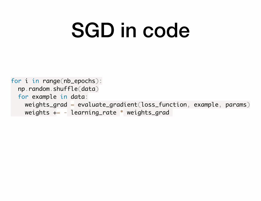
SGD in code

for i in range(nb_epochs): np.random.shuffle(data) for example in data: weights_grad = evaluate_gradient(loss_function, example, params) weights += - learning_rate * weights_grad

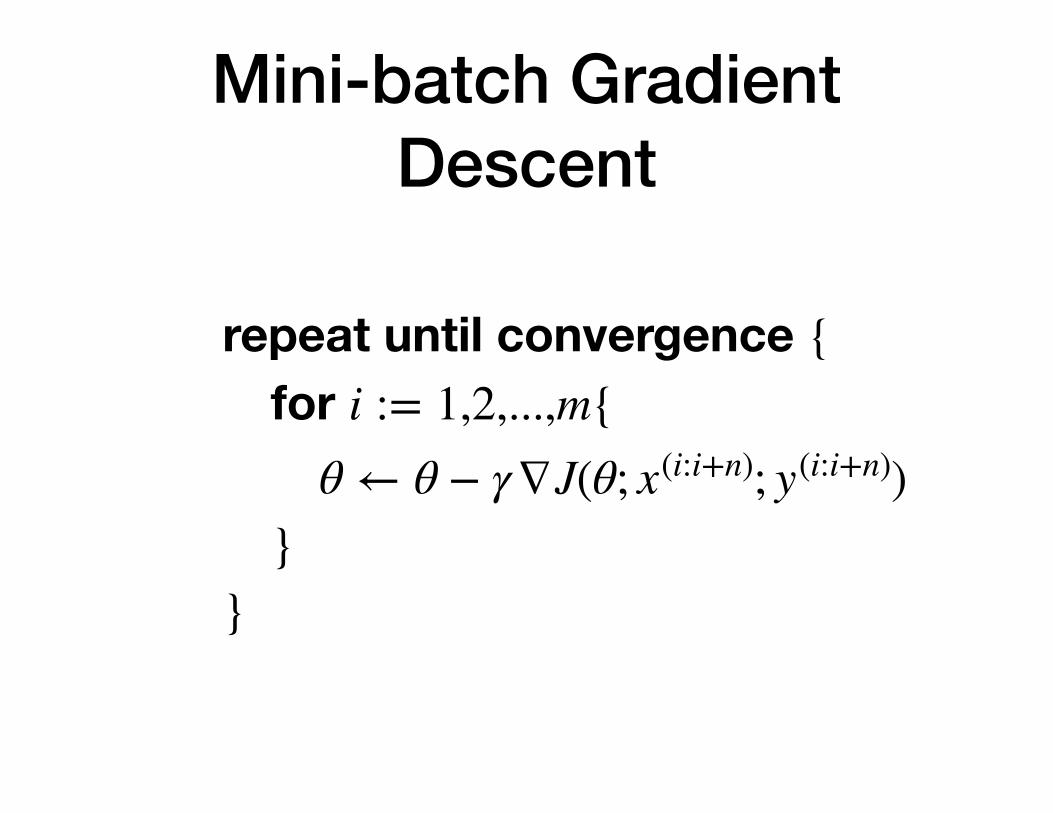
Mini-batch Gradient Descent

repeat until convergence {for i := 1,2,...,m{

θ ← θ − γ∇J(θ; x(i:i+n); y(i:i+n))}

}

Minibatch GD in code

for i in range(nb_epochs): np.random.shuffle(data) for batch in get_batches(data, batch_size=256): weights_grad = evaluate_gradient(loss_function, batch, params) weights += - learning_rate * weights_grad

What would be the ideal batch size?

• The size of the mini-batch is a hyper-parameter

• But it is not very common to cross-validate it!

• It is usually based on memory constraints (if any)

• In practice, we use powers of 2 because operations perform faster when their inputs are sized in powers of 2

• Rule of thumb: between 32-256

Challenges

Unlike in gradient descent, the value of the cost function does not necessarily

decrease

SGD performs frequent updates with a high variance that cause the objective

function to fluctuate

Choosing a proper learning rate can be difficult

• A learning rate that is too small leads to painfully slow convergence,

• A learning rate that is too large can hinder convergence and cause the loss function to fluctuate around the minimum or even to diverge.

Thresholds for adjusting learning rate should be defined in advance

• Adjusting the learning rate during training by e.g. annealing, i.e. reducing the learning rate according to a pre-defined schedule or when the change in objective between epochs falls below a threshold.

• These schedules and thresholds, however, have to be defined in advance and are thus unable to adapt to a dataset's characteristics.

The same learning rate applies to all parameter updates

• If our data is sparse and our features have very different frequencies, we might not want to update all of them to the same extent, but perform a larger update for rarely occurring features.

Minimizing highly non-convex functions are challenging

• Another key challenge of minimizing highly non-convex error functions common for neural networks is avoiding getting trapped in their numerous suboptimal local minima.

What computer systems can offer to resolve the

challenges?

Parallel Computer Memory Architectures

Shared memory architectures

• Each CPU can access the same memory space

• Multiple processors can operate independently but share the same memory resources

• Changes in a memory location effected by one processor are visible to all other processors.

Uniform Memory Access (UMA)

• Most commonly represented today by Symmetric Multiprocessor (SMP) machines

• Identical processors

• Equal access and access times to memory

• CC-UMA - Cache Coherent UMA

Non-Uniform Memory Access (NUMA)

• Often made by physically linking two or more SMPs

• One SMP can directly access memory of another SMP

• Not all processors have equal access time to all memories

• Memory access across link is slower

• CC-NUMA - Cache Coherent NUMA

Pros and Cons• Pros

• Global address space provides a user-friendly programming perspective to memory

• Data sharing between tasks is both fast and uniform due to the proximity of memory to CPUs

• Cons

• Lack of scalability between memory and CPUs

• Programmer responsibility for synchronization constructs that ensure "correct" access of global memory

Distributed Memory• Distributed memory systems require a communication

network to connect inter-processor memory

• Processors have their own local memory

• Because each processor has its own local memory, it operates independently

• When a processor needs access to data in another processor, it is usually the task of the programmer

Pros and Cons• Pros

• Memory is scalable with the number of processors.

• Each processor can rapidly access its own memory without interference.

• Cost effectiveness: can use commodity, off-the-shelf processors and networking.

• Cons

• The programmer is responsible for many of the details associated with data communication between processors.

• It may be difficult to map existing data structures, based on global memory, to this memory organization.

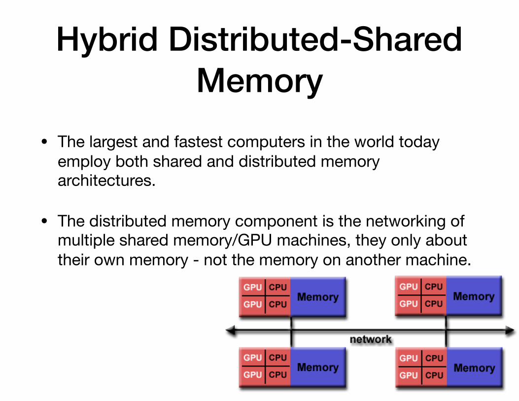
Hybrid Distributed-Shared Memory

• The largest and fastest computers in the world today employ both shared and distributed memory architectures.

• The distributed memory component is the networking of multiple shared memory/GPU machines, they only about their own memory - not the memory on another machine.

Parallel Programming Models

Shared Memory Model (without threads)

• In this programming model, processes/tasks share a common address space, which they read and write to asynchronously.

• Various mechanisms such as locks / semaphores are used to control access to the shared memory, resolve contentions and to prevent race conditions and deadlocks.

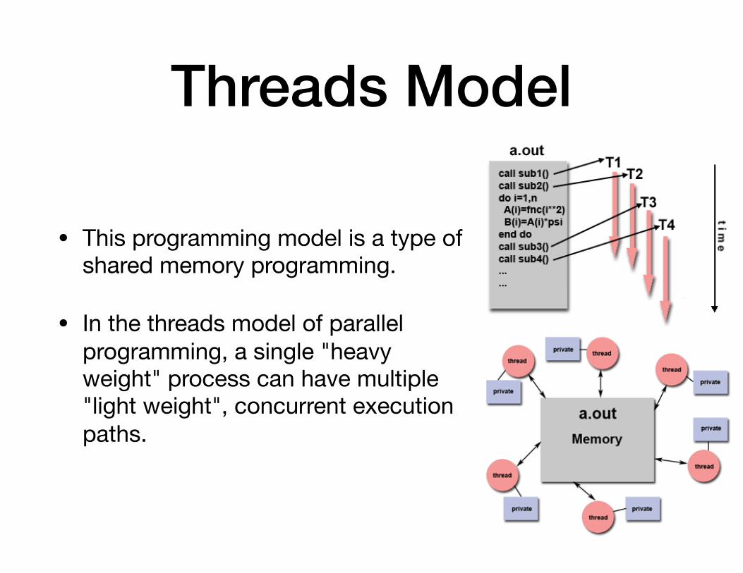
Threads Model

• This programming model is a type of shared memory programming.

• In the threads model of parallel programming, a single "heavy weight" process can have multiple "light weight", concurrent execution paths.

Parallel for loop in OpenMP

Distributed Memory / Message Passing Model

• A set of tasks that use their own local memory during computation.

• Tasks exchange data through communications by sending and receiving messages.

• Data transfer usually requires cooperative operations to be performed by each process.

Data Parallel Model• Address space is treated globally

• Most of the parallel work focuses on performing operations on a data set.

• A set of tasks work collectively on the same data structure, however, each task works on a different partition of the same data structure.

• Tasks perform the same operation on their partition of work, for example, "add 4 to every array element”.

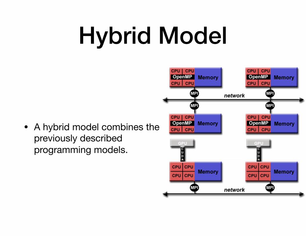
Hybrid Model

• A hybrid model combines the previously described programming models.

Now that we learned about computer systems approaches for

parallelization, how we can use them to parallelize SGD?

Lets discuss what are the core challenges?

When we need to add more parallelism to our computations?

• When training really deep models (16M parameters)

• On really large datasets (17B Examples)

What has been explored so far and what is the current trend

• Traditionally: Distributing linear algebra operations on GPUs,

• Now: How to use multiple machines

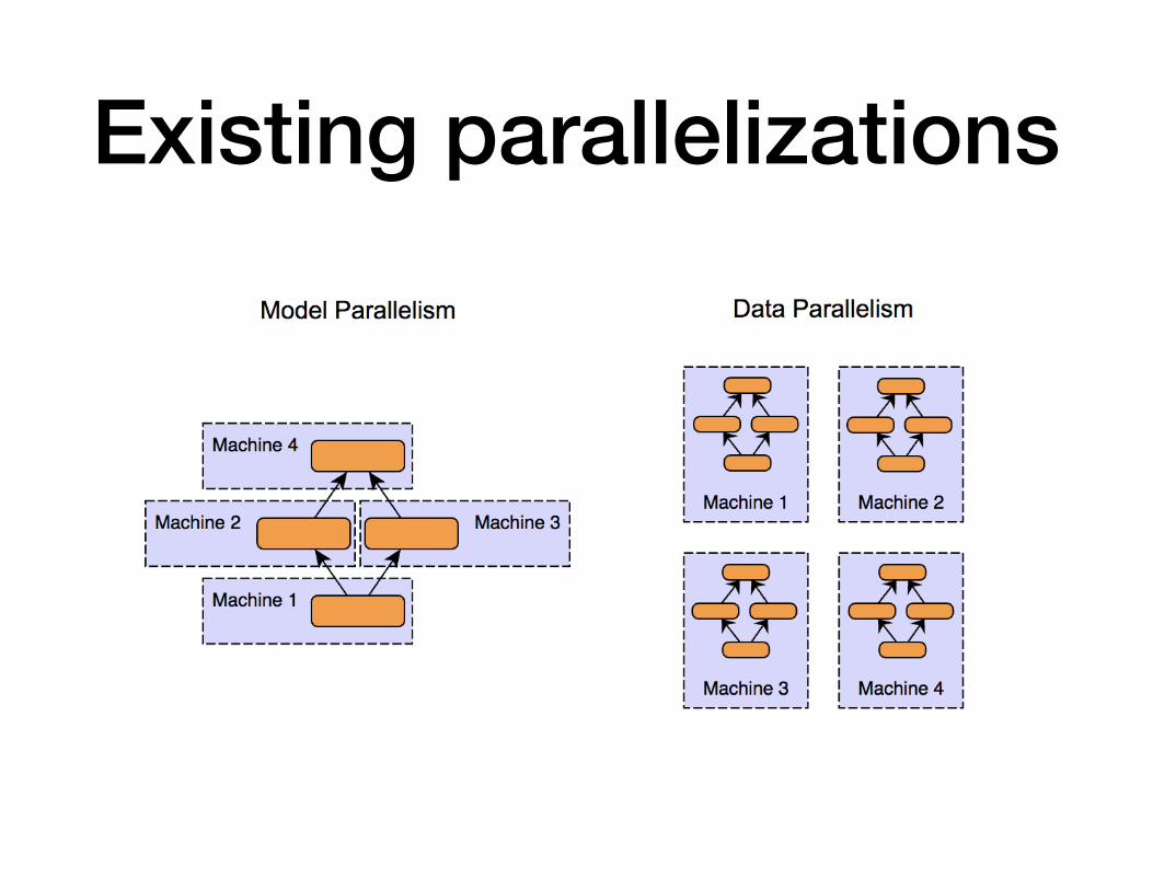
Existing parallelizations

We will mainly focus on data parallelism in the

rest of lecture

Parallel Gradient Descent

Parallel Gradient Descent

• Gradient computation is usually “embarrassingly parallel”

• Why?

• Consider, for example, empirical risk minimization as a learning algorithm:

repeat until convergence {θ ← θ − γ∇θJ(θ)

}

Remp(h) =1m

m

∑i=1

L(h(xi), yi) .

h = arg minh∈ℋ

Remp(h) .

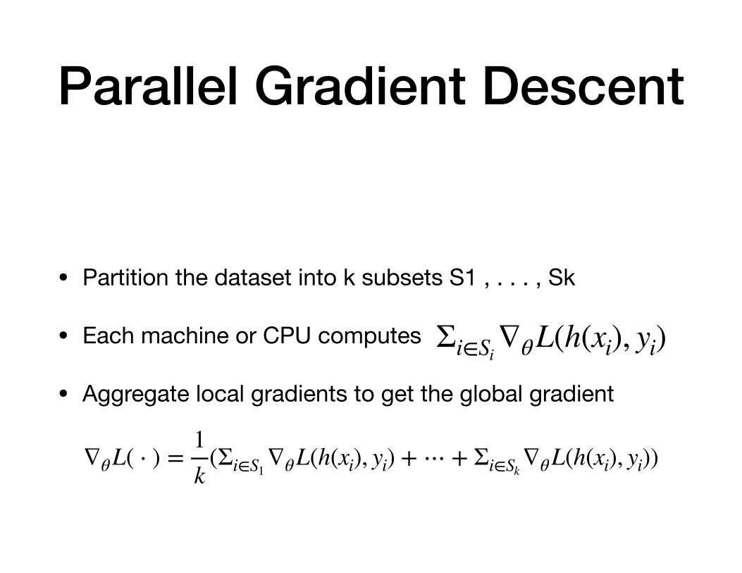
Parallel Gradient Descent

• Partition the dataset into k subsets S1 , . . . , Sk

• Each machine or CPU computes

• Aggregate local gradients to get the global gradient

Σi∈Si∇θL(h(xi), yi)

∇θL( ⋅ ) =1k

(Σi∈S1∇θL(h(xi), yi) + ⋯ + Σi∈Sk

∇θL(h(xi), yi))

Parallel Stochastic Gradient

• Computation of only depends on the i-th sample—usually cannot be parallelized.

• Parallelizing SGD is a not easy.

repeat until convergence {for i := 1,2,...,m{

θ ← θ − γ∇J(θ; x(i); y(i))}

}

∇J(θ; x(i); y(i))

Parallel Mini-batch SGD

• Let S = S1 ∪ S2 ∪ · · · ∪ Sk

• Calculate mini-batch updates in parallel

repeat until convergence {for i := 1,2,...,m{

θ ← θ − γ∇J(θ; x(i:i+n); y(i:i+n))}

}

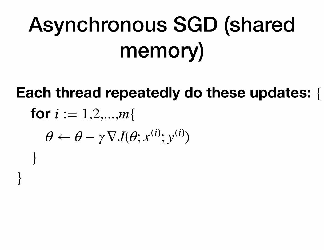
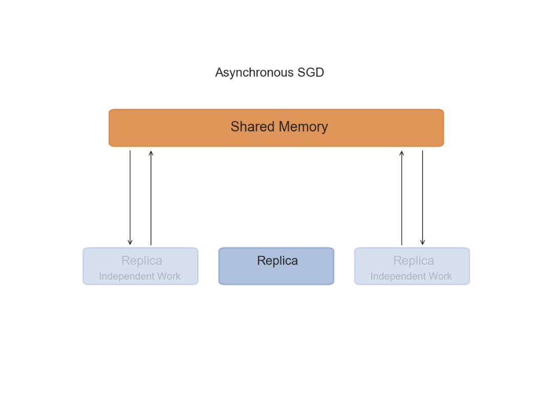
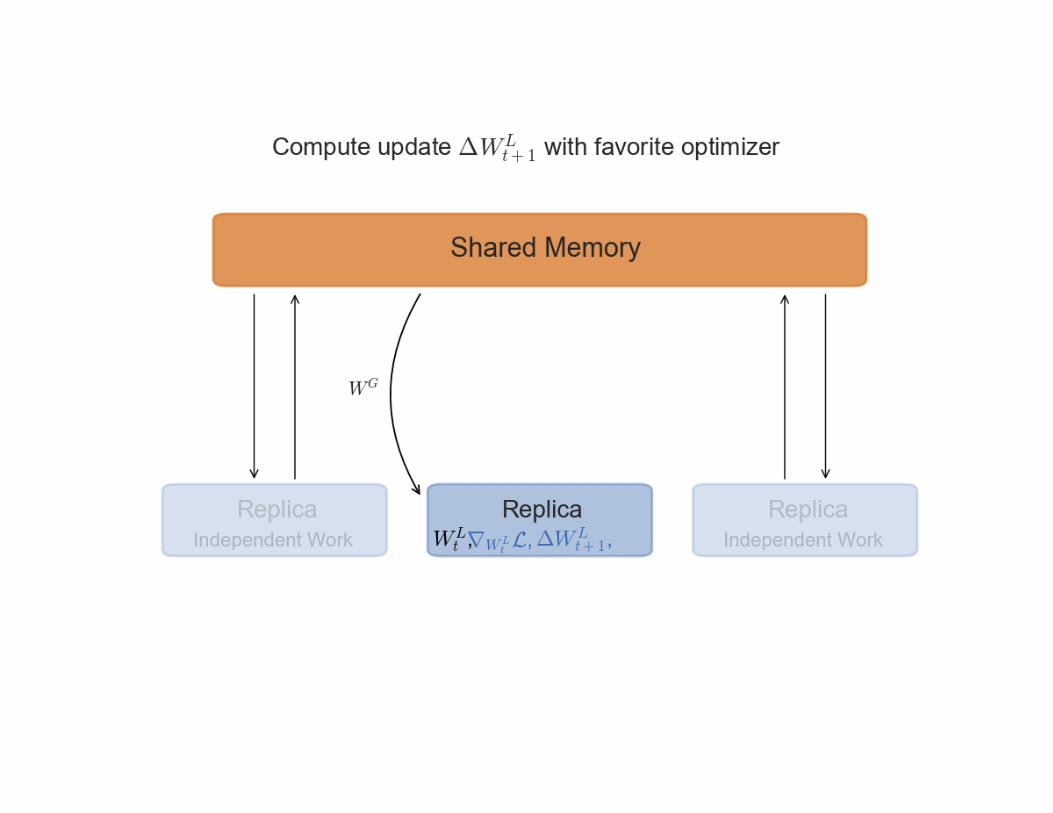
Asynchronous SGD (shared memory)

Each thread repeatedly do these updates: {for i := 1,2,...,m{

θ ← θ − γ∇J(θ; x(i); y(i))}

}

How using shared memory architecture?

• Main trick: in shared memory systems, every threads can access the latest gradient value

• Langford et al., “Slow learners are fast”. In NIPS 2009

• “Hogwild!: A Lock-Free Approach to Parallelizing Stochastic Gradient Descent”, NIPS 2011.

Synchronous Distributed SGD

Synchronous SGD

Pros

• The computation is completely deterministic.

• We can work with fairly large models and large batch sizes even on memory-limited GPUs.

• It’s very simple to implement, and easy to debug and analyze.

Cons• This path to parallelism puts a strong emphasis on HPC,

and the hardware that is in use.

• It will be challenging to obtain a decent speedup unless you are using industrial hardware.

• And even if you were using such a hardware, the choice of communication library, reduction algorithm, and other implementation details (e.g., data loading and transformation, model size, ...) will have a strong effect on the kind of performance gain you will encounter.

Asynchronous SGD

Pros

• The advantage of adding asynchrony to our training is that replicas can work at their own pace,

• without waiting for others to finish computing their gradients.

Cons

• We have no guarantee that while one replica is computing the gradients with respect to a set of parameters, the global parameters will not have been updated by another one.

• If this happens, the global parameters will be updated with stale gradients - gradients computed with old versions of the parameters.

How to solve staleness?

• [Zhang & al.] suggested to divide the gradients by their staleness. By limiting the impact of very stale gradients, they are able to obtain convergence almost identical to a synchronous system.

Zhang, W., Gupta, S., Lian, X., Liu, J.: Staleness-aware async-sgd for distributed deep learning. arXiv preprint arXiv:1511.05950. (2015)

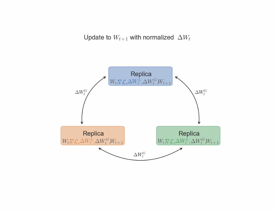
How to solve staleness?

• Each replica executes k optimization steps locally, and keeps an aggregation of the updates.

• Once those k steps are executed, all replicas synchronize their aggregated update and apply them to the parameters before the k steps.

Zhang, S., Choromanska, A.E., LeCun, Y.: Deep learning with elastic averaging sgd. In: Advances in neural information processing systems. pp. 685–693 (2015)

Implementation

What is the first decision then?

What is the decision?

• The first decision to make is how to setup the architecture of the system

What options do we have?

Parameter server

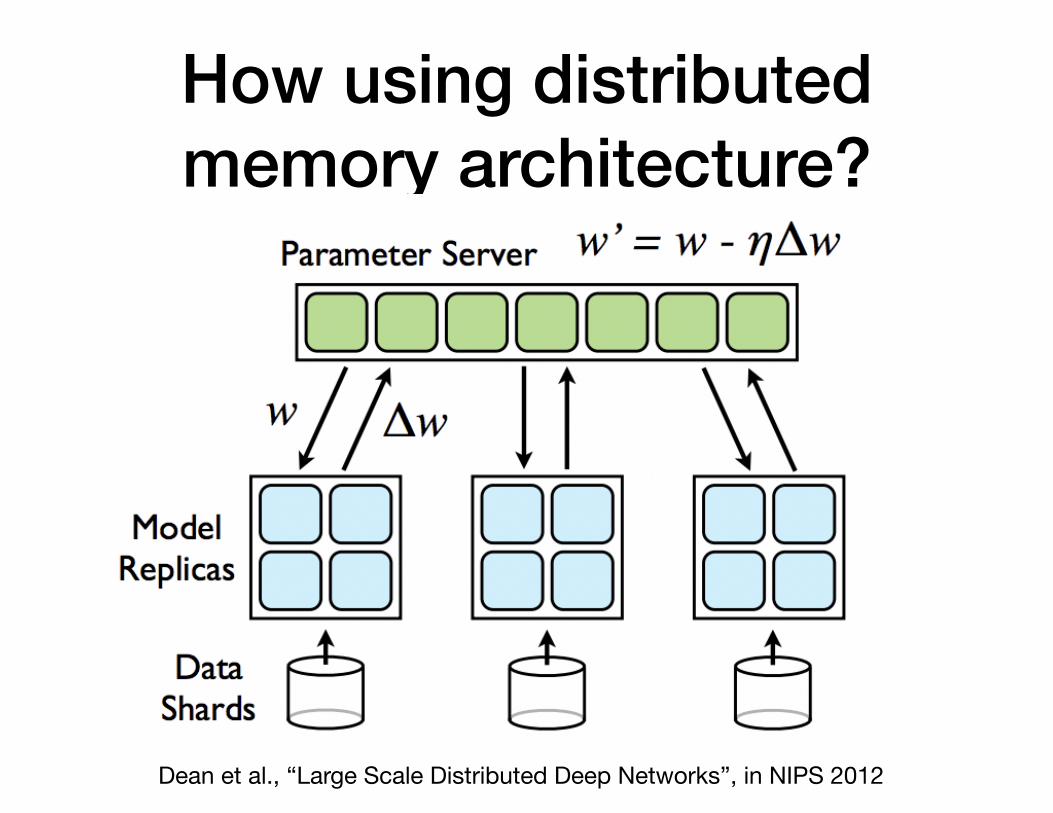
How using distributed memory architecture?

Dean et al., “Large Scale Distributed Deep Networks”, in NIPS 2012

Adding more hierarchy

Gupta, et. al, “Model Accuracy and Runtime Tradeoff in Distributed Deep Learning: A Systematic Study”, 2016

Mini-batch SG on distributed systems

• Can we avoid wasting communication time?

• Use non-blocking network IO: Keep computing updates while aggregating the gradient

Distributed mini-batch

Optimal Mini-Batch Size

Consider type of layers when parallelizing

• Conv layers parallelize particularly well given that they are quite compute heavy with respect to the number of parameters they contain.

• This is a desirable property of the network, since you want to limit the time spent in communication

• Convolutions achieve just that since they re-multiply feature maps all over the input.

Krizhevsky, A.: One weird trick for parallelizing convolutional neural networks. arXiv preprint arXiv:1404.5997. (2014)

Tricks

• Device-to-Device Communication

Tricks• Overlapping Computation

• E.g., synchronizing the gradients of the current layer while computing the gradients of the next one.

Tricks

• Approximate computing

Christopher De Sa, “High-Accuracy Low-Precision Training”, 2018.

Tricks

• Reduction algorithm

John Langford, “Allreduce for Parallel Learning”, 2017

Other applications?

Summary• We reviewed 3 variations of gradient descent

• We reviewed common challenges during training

• We examined computer system memory architectures and parallel programming models

• We discussed approaches to scale up SGD using parallel computations

• Next: Real-world case study about how Uber uses these ideas to make their deep learning tasks distributed over multiple machines to scale up training process