Scalable Data Cube Analysis over Big Data

Zhengkui Wang‡ Yan Chu ‡ ∗ Kian-Lee Tan‡

wangzhengkui@nus.edu.sg chuyan@hrbeu.edu.cn tankl@comp.nus.edu.sgDivyakant Agrawal§ Amr EI Abbadi§ Xiaolong Xu#

agrawal@comp.ucsb.edu amr@comp.ucsb.edu qlxucn@gmail.com

‡ National University of Singapore ∗ Harbin Engineering University§ University of California at Santa Barbara # AppFoilo Inc.

ABSTRACTData cubes are widely used as a powerful tool to provide multi-dimensional views in data warehousing and On-Line AnalyticalProcessing (OLAP). However, with increasing data sizes, it is be-coming computationally expensive to perform data cube analysis.The problem is exacerbated by the demand of supporting morecomplicated aggregate functions (e.g. CORRELATION, Statisti-cal Analysis) as well as supporting frequent view updates in datacubes. This calls for new scalable and efficient data cube analy-sis systems. In this paper, we introduce HaCube, an extension ofMapReduce, designed for efficient parallel data cube analysis onlarge-scale data by taking advantages from both MapReduce (interms of scalability) and parallel DBMS (in terms of efficiency).We also provide a general data cube materialization algorithm whichis able to facilitate the features in MapReduce-like systems towardsan efficient data cube computation. Furthermore, we demonstratehow HaCube supports view maintenance through either incremen-tal computation (e.g. used for SUM or COUNT) or recomputa-tion (e.g. used for MEDIAN or CORRELATION). We implementHaCube by extending Hadoop and evaluate it based on the TPC-Dbenchmark over billions of tuples on a cluster with over 320 cores.The experimental results demonstrate the efficiency, scalability andpracticality of HaCube for cube analysis over a large amount of datain a distributed environment.

1. INTRODUCTIONIn many industries, such as sales, manufacturing, transportation

and finance, there is a need to make decisions based on aggregationof data over multiple dimensions. Data cubes [13] are one suchcritical technology that has been widely used in data warehous-ing and On-Line Analytical Processing (OLAP) for data analysisin support of decision making.

In OLAP, the attributes are classified into dimensions (the group-ing attributes) and measures (the attributes which are aggregated)[13]. Given n dimensions, there are a total of 2n cuboids, eachof which captures the aggregated data over one combination of di-mensions. To speed up query processing, these cuboids are typi-cally stored into a database as views. The problem of data cube

materialization is to efficiently compute all the views (V) basedon the data (D). Fig. 1 shows all the cuboids represented as a cubelattice with 4 dimensions A, B, C and D.

In many append-only applications (no UPDATE and DELETEoperations), the new data (∆D) will be incrementally INSERTed orAPPENDed to the data warehouse for view update. For instance,the logs in many applications (like the social media or stocks) areincrementally generated/updated. There is a need to update theviews in a manner of one-batch-per-hour/day. The problem of viewmaintenance is to efficiently calculate the latest views while ∆Dare produced.

Both data cube materialization and view maintenance are com-putationally expensive, and have received considerable attention inthe literature [27][31][16][21]. However, existing techniques canno longer meet the demands of today’s workloads. On the onehand, the amount of data is increasing at a rate that existing tech-niques (developed for a single server or a small number of ma-chines) are unable to offer acceptable performance. On the otherhand, more complex aggregate functions (like complex statisticaloperations) are required to support complex data mining and sta-tistical analysis tasks. Thus, this calls for new scalable systems toefficiently support data cube analysis over a large amount of data.

Meanwhile, MapReduce (MR) [9] has emerged as a powerfulcomputation paradigm for parallel data processing on large-scaleclusters. Its high scalability and append-only features have madeit a potential target platform for data cube analysis in append-onlyapplications. Therefore, exploiting MR for data cube analysis hasbecome an interesting research topic. However, deploying an ef-ficient data cube analysis using MR is non-trivial. A naive imple-mentation of cube materialization and view maintenance over MRcan result in high overheads.

We first summarize the main challenges for cube analysis onlarge-scale data for developing an efficient cube analysis system.

• Given n dimensions in one relation, there are 2n cuboids thatneed to be computed in the cube materialization. An efficientparallel algorithm to materialize the cube faces two chal-lenges: (a) Given that some of the cuboids share commondimensions, is it possible to batch these cuboids to exploitsome common processing? (b) Assuming we are able to cre-ate batches of cuboids, how can we allocate these batchesor resources so that the load across the processing nodes isbalanced?

• View maintenance in a distributed environment introducessignificant overheads, as large amounts of data (either theold materialized data or the old base data) needs to be read,shuffled and written among the processing nodes and dis-tributed file system (DFS). Moreover, more and more appli-

arX

iv:1

311.

5663

v1 [

cs.D

B]

22

Nov

201

3

all

A

AB BC CD

ABCD

CB D

DA AC BD

ABC CDABCD DAB

Figure 1: A cube lattice with 4 dimensions: A, B, C and D

cations request to perform view updates more frequently thanbefore, shifting from one-update-per-week/month to almostone-update-per-day even per hour. It is thus critical to de-velop efficient view maintenance methods for frequent viewupdates, even realtime updates.

Therefore, in this paper, we are motivated to explore the tech-niques of developing new scalable data cube analysis systems byleveraging the MR-like paradigm, as well as to develop new tech-niques for efficient data cube analysis to broaden the applicationof data cubes primarily for append-only environments. Our maincontributions are as follows:

1. New system design and implementation: We present HaCube,an extension of MR, for large-scale data cube analysis. HaCube

tries to integrate the good features from both MR and parallel DBMS.HaCube extends MR to better support data cube analysis by inte-grating new features, e.g. a new local store for data reuse amongjobs, a layer with user-friendly interfaces and a new computationparadigm MMRR (MAP-MERGE-REDUCE-REFRESH). HaCube illus-trates one way to develop a scalable and efficient decision makingsystem, such that cube analysis can be utilized in more applications.

2. A General Cubing Algorithm: We provide a general and ef-ficient data cubing algorithm, CubeGen, which is able to completethe entire cube lattice using one MR job. We show how cuboidscan be batched together to minimize the read/shuffle overhead andsalvage partial work done. On the basis of batch processing princi-ple, CubeGen further leverages the ordering property of the reducerinput provided by the MR-like framework for an efficient materi-alization. In addition, we propose one load balancing approach,LBCCC to calculate the number of computation resources (reduc-ers) for each batch, such that the load to each reducer is balanced.

3. Efficient View Maintenance Mechanisms: We demonstratehow views can be efficiently updated under HaCube through eitherrecomputation (e.g. used for MEDIAN or CORRELATION) or in-cremental computation (e.g. used for SUM or COUNT). To thebest of our knowledge, this is the first work to address data cubeview maintenance in MR-like systems.

4. Experimental Study: We evaluate HaCube based on the TPC-D benchmark with more than two billions tuples. The experimentalresults show that HaCube has significant performance improvementover MR.

The rest of the paper is organized as follows. Section 2 pro-vides the preliminary knowledge of MR computation paradigm. InSection 3, we provide an overview of HaCube. Sections 4 and 5present our proposed cube materialization and view maintenanceapproaches. We discuss the fault tolerance and other issues in Sec-tion 6, and report our experimental results in Section 7. In Section8 and Section 9, we review some related works and conclude the

paper.

2. PRELIMINARIESIn this section, we provide a brief overview of the MR com-

putation paradigm. MapReduce has emerged as a powerful par-allel computation paradigm [9]. It has been widely used by var-ious applications such as scientific data processing [24][25][26],text processing [17][22], data mining [7] [30] and machine learn-ing [8] [12] and so on. MapReduce has several advantages whichmake it an attractive platform for large-scale data processing, suchas its high scalability (scalability of thousands of machines), goodfault tolerance (automatic failure recovery by the framework), ease-of-programming (simple programming logic) and high integrationwith cloud(availability to every user and low expense in a pay-as-you-go cloud model).

Under the MapReduce framework, the system architecture of acluster consists of two kinds of nodes, namely, the NameNode andDataNodes. The NameNode works as a master of the file system,and is responsible for splitting data into blocks and distributing theblocks to the data nodes (DataNodes) with replication for fault tol-erance. A JobTracker running on the NameNode keeps track of thejob information, job execution and fault tolerance of jobs executingin the cluster. A job may be split into multiple tasks, each of whichis assigned to be processed at a DataNode.

The DataNode is responsible for storing the data blocks assignedby the NameNode. A TaskTracker running on the DataNode is re-sponsible for the task execution and communicating with the Job-Tracker.

The computation of MR follows a fixed model with a map phase,followed by a reduce phase. Users can set their own computationlogic by writing the map and reduce functions in their applications.

Map Phase: The MR library is responsible for splitting the datainto chunks from the distributed system (DFS) and distributing eachchunk to a processing unit (called mapper) on different nodes. Themap function is used to process (key,value) pairs (k1,v1) read fromdata chunks and, after applying the map function, then emits a newset of intermediate (k2,v2) pairs.

The MR library sorts and partitions all the intermediate data intor partitions based on the partitioning function in each mapper,where r is the number of processing units (called reducers) forfurther computation. The partitions with the same partition num-ber are shuffled to the same reducer. We note that MR randomlychooses the free reducer to process the partitions.

Reduce Phase: The MR library merge-sorts all the (key, value)pairs based on the key first. Then, the globally sorted data are sup-plied to the reduce function iteratively. After the reduce process,the reducer emits new (k3,v3) pairs to the DFS.

When one job finishes, all intermediate data are removed fromthe mappers and reducers. If another job wants to use the samedata, it has to reload the data from the DFS again.

3. HACUBE: THE BIG PICTURE

3.1 ArchitectureFigure 2 gives an overview of the basic architecture of HaCube.

We implement HaCube by modifying Hadoop which is an opensource equivalent implementation of MR [1]. Similar to MR, allthe nodes in the cluster are divided into two different types of func-tion nodes, including the master and processing nodes. The masternode is the controller of the whole system and the processing nodesare used for storage as well as computation.

Master Node: The master node consists of two functional layers:

Job Scheduler Task

Scheduling

Factory

Map

Merge

Local StoreMapper

...

Master Node

Cube Analyzer

Cube Planner

Cube Converting Layer

Task Scheduler

Execution Layer

OR

DB

Distributed

File

System

Cube Request

Submission

Processing Node

RefreshReduce

Reducer

OR

DB

Distributed

File

System

Map

Merge

Local StoreMapper

RefreshReduce

Reducer

...

Processing Node

Figure 2: HaCube Architecture

1. The cube converting layer contains two main components:Cube Analyzer and Cube Planner. The cube analyzer is de-signed to accept the user request of data cube analysis, analyze thecube, such as figuring out the cube id (the identifier of the cubeanalysis application), analysis model (materialization or view up-date), measure operators (aggregation function), and input and out-put paths etc.

The cube planner is developed to convert the cube analysis re-quest into an execution job (either a materialization job or a viewupdate job). The execution job is divided into multiple tasks eachof which handles part of the cuboid calculation. The cube plan-ner consists of several functional components such as the execu-tion plan generator (combine the cuboids into batches to reduce theoverhead), and load balancer (assign the right number of computa-tion resources for each batch).

2. The execution layer is responsible for managing the execu-tion of jobs passed from the cube converting layer. It has threemain components: job scheduler, task scheduler and task

scheduling factory. We use the same job scheduler as in Hadoopwhich is used to schedule different jobs from different users. In ad-dition, we add a task scheduling factory which is used to record thetask scheduling information of a job which can be reused in otherjobs. Furthermore, we develop a new task scheduler to schedule thetasks in terms of the scheduling history stored in the task schedul-ing factory rather than the random scheduler used in MR.

Processing Node: A processing node is responsible for the taskexecution assigned from the master node. Similar to MR, each pro-cessing node contains one or more processing units each of whichcan either be a mapper or a reducer. Each processing node has aTaskTracker which is in charge of communicating with the mas-ter node through heartbeats, reporting its status, receiving the task,reporting the task execution progress and so on. Unlike MR, thereis a Local Store built at each processing node running reduc-

ers. The local store is developed to cache useful data of a job inthe local file system of the reducer node. It is a persistent storagein the local file system and will not be deleted after a job execu-tion. In this way, tasks (possibly from other jobs) assigned to the

same reducer node are able to access the local store directly fromthe local file system.

3.2 Computation ParadigmHaCube inherits some features from MR, such as data read/proce-

ss/write format of (key, value) pairs, sorting all the intermediatedata and so on. However, it further enhances MR to support anew computational paradigm. HaCube adds two optional phases- a Merge phase and a Refresh phase before and after the Re-

duce phase - to support the MAP-MERGE-REDUCE-REFRESH(MMRR) paradigm as shown in Fig. 2.

The Merge phase has two functionalities. First, it is used to cachethe data from the reduce input to the local store. Second, it is devel-oped to sort and merge the partitions from mappers with the cacheddata in the local store. The Refresh phase is developed to performfurther computations based on the reduce output data. Its function-alities include caching the reduce output data to the local store andrefreshing the reduce output data with the cached data in the lo-cal store. These two additional phases are intended to fit differentapplication requirements for efficient execution support.

As mentioned, these two phases are optional for the jobs. Userscan choose to use the original MR computation or MMRR compu-tation. More details can be found in Section 5 about how MMRRbenefits the data cube view maintenance.

4. CUBE MATERIALIZATIONIn this section, we provide our proposed data cubing algorithm,

CubeGen, under the MR-like systems. We first present some prin-ciples of sharing computation through cuboid batching followed bya batched generator. We then introduce the load balancing strategyfollowed by the detail implementation of CubeGen. For simplicity,we assume that we are materializing the complete cube. Note thatour techniques can be easily generalized to compute a partial cube(compute only selective cuboids). We also omit the cuboid “all"from the lattice. This special cuboid can be easily handled throughan independent processing unit.

4.1 Cuboid Computation Sharing

To build the cube, computing each cuboid independently is clearlyinefficient. A more efficient solution, which we advocate, is tocombine cuboids into batches so that intermediate data and com-putation can be shared and salvaged.

We provide the following lemma as a formal basis for combiningand batching the cuboids computation under MR-like systems.

LEMMA 1. Let A and B be a set of dimensions such that A⋂

B=/0. In MR-like systems, given cuboids A and AB, A can be combinedand processed together with AB, once AB is set of the key and ispartitioned by A in one MR job. A is referred to as the ancestor ofAB (denoted as A ≺ AB). Meanwhile, AB is called the descendantof A. Note that the ancestor and descendant require them share thesame prefix.

PROOF. Without loss of generality, we assume A = d1, ..., dxand B = dy, ..., dy+z where di is one dimension. When AB is pro-cessed, the output key in the mapper can be set as the group-bydimensions of AB (d1, ..., dx, dy, ..., dy+z) on which the (k,v) pairsare further sorted based on AB. Partitioning AB based on A guaran-tees that all the same group-by cells in A are shuffled to the samereducer where A is also in a sorted order. Therefore, we can processA as well while AB is processed.

The above results can be generalized using transitivity: Since wecan combine the processing of the pair of cuboids {A,AB} and thepair {AB,ABC}, we can also combine the processing of the threecuboids {A, AB, ABC}. Thus, given one cuboid, all its ancestorscan be calculated together as a batch. For instance, in Fig. 1, asA≺ AB≺ ABC≺ ABCD, the cuboids A, AB, ABC can be processedwith ABCD. Note that BC cannot be processed with ABCD becauseBC ⊀ ABCD.

Given a batch, the principle to calculate this batch is to set thesort dimensions as the key and partition the (k,v) pairs based onthe partition dimensions in the key in the MR-like paradigm. Weformally define these two dimension classes below:Definition 1 Sort Dimensions: The dimensions in cuboid A arecalled the sort dimensions if A is the descendant of all other cuboidsin one batch.Definition 2 Partition Dimensions: The dimensions in cuboid Aare called the partition dimensions if A is the ancestors of all othercuboids in one batch.

For instance, given the batch {A,AB,ABC,ABCD}, ABCD and Acan be set as the sort and partition dimensions respectively.

The benefits of this approach are: 1) In the reduce phase, thegroup-by dimensions are all in sorted order for every cuboid in thebatch, since MR would sort the data before supplying to the reducefunction. This is an efficient way of cube computation since it ob-tains sorting for free and no other extra sorting is needed beforeaggregation. 2) All the ancestors do not need to shuffle their ownintermediate data but use their descendant’s. This would signifi-cantly reduce the intermediate data size, and thus remove a lot ofdata sort/partition/shuffle overheads.

To achieve good performance, we need to address two issues.First, how can we find the minimum number of batches from the2n cuboids? As more cuboids are combined together, the shufflingoverhead incurred for data shuffling will be reduced. Second, howcan we balance the load to assign the right number of computationresources to each batch? As different batches may have differentcomputation complexity and data size, it is not optimal to evenlyassign the computation resources to each batch. Before providingthe detailed algorithm for CubeGen, we first introduce how it solvesthe aforementioned challenges by developing a plan generator

and a load balancer.

Figure 3: A directed graph of expressing 4 dimensions A, B, Cand D

4.2 Plan GeneratorThe goal of the plan generator is to generate the minimum num-

ber of batches among the 2n-1 cuboids, excluding “all′′. The plangenerator first divides the 2n-1 cuboids into n groups each of whichconsists of the cuboids with i dimension attributes. For instance,given the cube lattice with 4 dimension attributes in Figure 1, it canbe divided into 4 groups (from the bottom of the lattice to the top)as follows: G1 = {A,B,C,D}, G2 = {AB,BC,CD,DA,AC,BD},G3 = {ABC,BCD,CDA, DAB}, G4 = {ABCD}.

Recall that one cuboid can be batched with all its sub-cuboids.Thus, we adopt a greedy approach to combine one cuboid with asmany of its ancestors as possible. Initially, all the cuboids in eachgroup are marked as available. Each construction of a batch startswith one available cuboid, α , from the non-empty group with themaximum number of dimensions. It then searches all the avail-able ancestors of α from other groups that can be batched together.For instance, the first batch construction starts with ABCD in theexample above (Since ABCD has 4 dimensions, it is the one withmaximum number of dimensions). Note that since cuboid α hasdifferent permutations (e.g. ABCD can also be permuted as ABDC,ACBD, BCDA, CDAB, DABC etc.), the algorithm enumerates allpermutations and the one with the maximum number of availableancestors will be chosen. Once one batch is constructed, all thecuboids in this batch are deleted from the search space and becomeunavailable. Similarly, the next batch construction is conductedamong the remaining available cuboids. The construction finisheswhen there are no available cuboids left.

The approach we adopt to generate the batches is similar to theone proposed in [16]. Lee et al. provide an extensive proof that the

algorithm is able to generate Cd n

2 en batches which is the minimum

number. Recall that there are Cd n

2 en cuboids in group Gd n

2 e and thatnone of them can be combined with each other. So there are atleast C

d n2 e

n batches. Interested readers are referred to [16] for moredetails.

To improve the efficiency of batch construction, two optimiza-tions are adopted to reduce the search space.

• First, recall that for a set of dimensions, we need to com-pute a batch for each permutation. This, however, may notbe necessary. In fact, when all the sub-cuboids of a particularpermutation are available, we know that we have found a per-mutation with the maximum number of sub-cuboids. There-fore, as soon as we encounter such a permutation, we do notneed to continue the search for this set of dimensions.

• Second, we organize all the dimensions as one directed graphsuch that one dimension points to another and we refer tothe distance between two adjacent dimensions as one hop.For instance, given 4 dimensions A, B, C and D, they can

all

1:A

5:AB 6:BC 7:CD

15:ABCD

3:C2:B 4:D

8:DA 9:AC 10:BD

11:ABC 13:CDA12:BCD 14:DAB

Figure 4: The numbered cube lattice with execution batches

be expressed as a directed graph such that A, B, C and Dpoint to B, C, D and A respectively as shown in Figure 4 (b).During permutation enumeration, changing from A to B or Cis referred as moving one hop or two hops from A.

To find the permutation of a cuboid α with the maximumnumber of sub_cuboids, the enumeration starts from the per-mutation that is obtained by moving the equivalent numberof hops for each dimension of the unavailable cuboid in thesame group. This is to guarantee that, most likely, the firstsearch permutation is the one we need to reduce the searchspace. For instance, assume that the first batch is generated asABCD, ABC, AB and A. Then the next initial permutation fora new batch is BCD which is computed through moving onehop for each dimension in the unavailable cuboid ABC. It isclear that the new batch can be generated with BCD (since allits sub_cuboids are available) and there is no need to searchother permutation of BCD.

In the same way, the batches of CDA and DAB will be gener-ated. These two optimizations speed up the batch construc-tion.

Figure 4 shows an example of the generated batches using thedotted lines.

4.3 Load BalancerGiven a set of batches from the plan generator, the load balancer

is used to assign the right number of computation resources to eachbatch to balance the load.

We argue that existing works (like [20]) that balance the batchesby evenly assigning the computation resources may not always bea good choice.

• First, it requires users to provide very specific informationabout the application data to be able to estimate a model tofind the balanced batches.

• Second, the cuboids may not be combined into balanced batches.

• Third, in a MR-like system, it is hard to make a precise costestimate of each batch. For instance, the total cost of eachbatch includes the following main parts: the data shufflingcost (shuffling the intermediate data from mappers to reduc-ers), the sorting cost (all the intermediate data are sorted),data processing cost (applying the measure function to eachcuboid in a batch) and data writing cost (writing the views tothe file system). It is hard to estimate each of these compo-nent costs and even harder to evaluate the total cost of each

batch (as this requires setting the appropriate weights whencombining these components).

Therefore, the load balancing among different batches becomesa very tricky and challenging problem in MR-like systems.

In this paper, we propose a novel load balancing scheme LBCCC(short for Load Balancing via Computation Complexity Compari-son) to assign the right number of computation resources to eachbatch. Intuitively, LBCCC adopts a profiling based approach wherea learning job (we refer as CCC - Computation Complexity Com-parison job ) is first conducted on a small test dataset to evaluatethe computation overhead relationship between each batch and thengenerate the number of reducers for each batch that are proportionalto computation overhead for the actual CubeGen jobs. The compu-tation cost relationship is estimated through the execution compar-isons when each batch is provided the same number of computationresources. The execution time relationship over the same compu-tation resource indicates the entire batch processing overhead rela-tionship, thus helps to make an accurate load balancing decision.

In particular, LBCCC first conducts the CCC job, a cube materi-alization learning job, on a small test dataset where each batch isassigned to one reducer. It then records and utilizes the executiontime of each batch to estimate the computation overhead relation-ship among different batches.

The test data can be obtained either by sampling or producedwithin a time window provided by users. Note that the samplingcan be accomplished during the CCC job, since the MR frameworkprovides APIs for sampling data directly. Therefore, by default,we use the sampling approach provided by the Hadoop API whereone tuple is sampled from every s records. Users can also plugin their own sampling algorithm easily. The sampling algorithmshave been widely studied in the literature. Since it is not our focuson studying how to choose or design a good sampling algorithm,we shall not discuss it here and more sampling algorithms can befound in [11].

In the CCC job, given a set of base data, the mapper conductssampling on it. For each sampling tuple, the mapper emits multiple(key,value) pairs each of which is for one batch. Then the CCC jobshuffles the pairs that belong to the same batch to one particularreducer. Given b batches, the CCC job uses b reducers each ofwhich is in charge of processing one batch. The implementation ofthe CCC algorithm is similar to the CubeGen algorithm providedin Algorithm 1 except for the number of reducers assigned to eachbatch. The algorithm detail can be found in section 4.4.

The CCC learning job records the execution time Ti for pro-cessing batch Bi. Based on the execution time recorded, the loadbalancer generates the resources assignment plan for each batch.Given r reducers, the right number of reducers, Ri for batch Bi canbe calculated as follows:

Ri =Ti∗r

∑b−1j=0 Tj

The load balancer integrates this plan into the CubeGen algo-rithm to balance the load. The experimental results show that LBCCCis able to balance the load very well.

We note that this evaluation only needs to be done once beforethe initial cube materialization and is used for subsequent jobs inthe same application. Furthermore, performing the CCC job ischeap as only b reducers are needed. Note that the load balancercan support different kinds of batching approaches. Therefore, theLBCCC load balancing scheme is general and effective for differentcubing algorithms.

4.4 Implementation of CubeGen

Algorithm 1: CubeGen AlgorithmFunction: Map(t)

1 # t is the tuple value from the raw data2 Let B (resp. Ii) be the batch set with B0, B1, ..., Bb−1 (resp. the

identifier of batch Bi)3 for each Bi in B do4 k (resp. v)⇐ get sort dimensions (resp. the measure m) in Bi

from t5 # If there are multiple measures (e.g. m1,m2), then v⇐ (m1,m2)6 v.append(Ii); emit(k,v);

Function: Partitioning(k,v)7 Let Ri (resp. attr) be the number of reducers (resp. the partition

dimensions) for Bi8 Si ⇐ ∑

i−1j=0 R j

9 return Si + hash(attr,Ri);Function: Reduce/Combine (k,{v1,v2, ...,vm})

10 Let C (resp. M) be the cuboid set in the batch identifier (resp. theaggregate function)

11 for Ci in C do12 if Ci is ready then13 k′′ (resp. v′′)⇐ get the group-by dimensions in Ci (resp.

M(v1, ...,vm,v′1, ...,v

′k, ...))

14 # Perform multiple aggregate functions e.g. (M1,M2) here:v′′1 ⇐M1(v1, ...,vm,v

′1, ...,v

′k, ...) and v′′2 ⇐

M2(v1, ...,vm,v′1, ...,v

′k, ...)

15 emit(k′′,v′′);

16 else17 Buffer the measure for aggregation

Consider the batch plan B (B0, B1, ..., Bb−1) generated from theplan generator and the load balancing plan R=(R0, R1, ..., Rb−1)where the Ri is the number of reducers assigned for batch Bi. GivenB and R, the proposed CubeGen algorithm materializes the entirecube in one job and its pseudo-code is provided in Algorithm 1.

Map Phase: The base data is split into different chunks each ofwhich is processed by one mapper. CubeGen parses each tuple andemits multiple (k,v) pairs each of which is for one batch (lines 3-6).The sort dimensions in the batch are set as the key and the measureis set as the value.

To distinguish which (k,v) pair is for which batch with whichcuboids, we add a batch identifier appended after the value. Theidentifier is developed as one Bitmap with 2n bits where n is thenumber of dimensions and each bit corresponds to one cuboid.First, we number all the 2n cuboids from 0 to 2n-1. Second, ifthe cuboid is included in one batch, its corresponding bit is set as 1,otherwise 0. For instance, Fig. 4 depicts an example of a numberedcube lattice. Assume that B0 consists of cuboids {A,AB,ABC andABCD}. The identifier for B0 is set as ‘10001000 00100010′.

The partitioning function partitions the pairs to the appropriatepartition based on the identifier and the load balancing plan R.CubeGen first schedules the data into the right range of reducers.Recall that the batch Bi is assigned Ri reducers. Therefore, theassigned reducers for batch Bi are from ∑

i−1j=0 R j to ∑

i−1j=0 R j+Ri-1.

Then the (k,v) pairs are hash partitioned among these Ri reducersaccording to the partition dimensions in the key (lines 7-9).

Reduce Phase: In the Reduce phase, the MR library sorts allthe (k,v) pairs based on the key and passes them to the reduce func-tion. Each reducer obtains its computation tasks (the cuboids in thebatch) by parsing the batch identifier in the value. The reduce func-tion extracts the measure and projects the group-by dimensions foreach cuboid in the batch. For the descendant cuboid, the aggre-gation can be performed directly based on input tuple, since eachinput tuple is one complete group-by cell. For other cuboids, the

Algorithm 2: A Refresh Job in MRFunction: Map(t)

1 # t is the tuple value from either V or ∆V2 k (resp. v)⇐ get dimensions (resp. aggregate value) from t;3 emit(k,v)

Function: Reduce(k, {v1,v2})4 emit(k,M(v1,v2))

measures of the group-by cell are buffered until the cell receivesall the measures it needs for aggregation (lines 11-17). We developmultiple file emitters to write different aggregated results to differ-ent destinations.

Note that if the (k,v) pairs can be pre-aggregated in the map

phase, users can specify a combine function to conduct a first roundaggregation. The combine function is normally similar to the re-duce function as shown in lines 10-17, but only aggregates the pairswith the same key. This pre-aggregation is able to reduce the datashuffle size between mappers to reducers.

We emphasize that if there are muliple measures (e.g. m1, m2, ...,mn) and multiple aggregate functions (M1,M2, ..,Mm), they can beprocessed in the same MR job as shown in the line 5 and 14 in Al-gorithm 1. Compared to the naive solution, CubeGen minimizes thecube materialization overheads by sharing the data read/shuffle/compu-tation to the maximum, which obtains significant performance im-provement as we shall see in Section 7.

5. VIEW MAINTENANCEThere are two different manners to update the views, namely re-

computation and incremental computation. Recomputation com-putes the latest views by reconstructing the cube based on the entirebase data D and ∆D. In append-only applications, this manner isnormally used for the holistic aggregate functions, e.g. STDDEV,MEDIAN, CORRELATION and REGRESSION [13].

Incremental computation, on the other hand, updates the viewsusing only V and ∆D in two steps: 1.) In the propagate step, a deltaview ∆V is calculated based on the ∆D. 2.) In the refresh step,the latest view is obtained by merging V and ∆V without visitingD [18]. In append-only applications, this manner is normally usedfor the distributive and algebraic aggregate functions, e.g. SUM,COUNT, MIN, MAX and AVG [13]. Note that the update for thesefunctions can also be conducted through recomputation.

5.1 Supporting View Maintenance in MRTo support recomputation in MR, when ∆D is inserted, the latest

views can be calculated by issuing one MR job using our CubeGenalgorithm to reconstruct the cube over D∪∆D. The key problemwith such a MR-based recomputation view updates is that recon-struction from scratch in MR is expensive. This is because the basedata (which is large and increases in size at each update) has to bereloaded to the mappers from DFS and shuffled to the reducers foreach view update, which incur significant overheads.

To support incremental computation in MR, the latest views canbe calculated by issuing two MR jobs. The first propagate job gen-erates ∆V from ∆D using our proposed CubeGen algorithm. Thesecond refresh job merges V and ∆V as shown in Algorithm 2.However, this would incur significant overheads. For instance, thematerialized ∆V from the propagate job has to be written back toDFS, reloaded from DFS again and shuffled from mappers to re-ducers in the refresh job. Likewise, V has to be reloaded and shuf-fled around in the refresh job. Therefore, it is highly expensive tosupport view update operations directly over the traditional MR.

a1,3

a2,4

a1,9

a2,5

a1,5

a2,7

Merge

Reduce:Median

a1,3

a1,5

a1,9

a2,4

...

Cache

Local Store

output

a1,5

a2,5

P0_0 P0_1 P0_2

Reducer 0

(a) MEDIAN: Cube Materialization (Map-Merge-Reduce)

a1,2

a2,1

a1,4

a2,3

Merge

Reduce:Median

a1,3

a1,5

a1,9

...

Local Store

output

a1,4

a2,4

Merge

Update

a1,2

a1,3

a1,4

a1,5

a1,9...

P0_0 P0_1

Reducer 0

(b) MEDIAN: View Maintenance (Map-Merge-Reduce)

Figure 5: Recomputation for MEDIAN in HaCube

5.2 HaCube Design PrinciplesHaCube avoids the aforementioned overheads through storing

and reusing the data between different jobs. We extend MR to adda local store in the reducer node which is intended to store usefuldata of a job in the local file system. Thus, the task shuffled to thesame reducer is able to reuse the data already stored there. In thisway, the data can be read directly from the local store (and thussignificantly reducing the overhead that would have been incurredto read the data from DFS and shuffle them from mappers).

We further extend MR to develop a new task scheduler to guaran-tee that the same task is assigned to the same reducer node and thusthe cached data can be reused among different jobs. Specifically,the task scheduler records the scheduling information by storinga mapping between the data partition number (corresponds to thetask) and the TaskTracker (corresponds to the reducer node) andputs it to the task scheduling factory from one job. When a newjob is triggered to use the scheduling history from previous jobs,the task scheduler fetches and adopts the scheduling informationfrom the factory to distribute the tasks. The scheduler automati-cally checks the situation of the over-loaded nodes and re-assignsthe task to a nearby processing node.

In addition, two computation phases (Merge and Refresh) areadded to conduct more computation with the cached data locally.The Merge phase is added to either cache the intermediate reduceinput data in one job or preprocess the data between the newly ar-riving data and cached data before the Reduce phase. The Refreshphase is added to either cache the reduce output data in one job orpostprocess the reduce output result with the cached data after theReduce phase.

5.3 Supporting View Maintenance in HaCube

5.3.1 RecomputationThe recomputation view update can be efficiently supported in

HaCube using a Map-Merge-Reduce (MMR) paradigm. We demon-strate this procedure through one running example by introducingthe cube materialization and update jobs.

In the first cube materialization job, HaCube is triggered to cachethe intermediate reduce input data to the local store in the Merge

phase, such that this data can be reused during the view updatejob. For instance, Fig. 5(a) shows an example of calculating thecuboid A for MEDIAN. Assume that reducer 0 is assigned to pro-cess cuboid A. In this job, each mapper emits one sorted partitionfor reducer 0, such as P0_0,P0_1 and P0_2. Here, each partition isa sequence of (dimension-value, measure-value) pairs, e.g., (a1, 3),(a2, 4). Recall that once these partitions are shuffled to the reducer0, it first performs a merge-sort (the same as MR does) to sort allthe partitions based on the key in the Merge phase. The sorted datais further supplied to the reduce function to calculate the MEDIANfor each group-by cell (e.g. < a1,5 > and < a2,5 >) where thisview will be written to DFS.

Different to MR (which deletes all the intermediate data afterone job), since recomputation requires the base data for update,HaCube caches the sorted reduce input data in the Merge phasefor subsequent reuse. This caching operation is conducted whilethe Reduce phase finishes, which guarantees the atomicity of theoperation - if the reduce task fails, the data will not be written tothe local store. Meanwhile, the scheduling information is recorded.

A view update job is launched when ∆D is added for view up-dates. Intuitively, this job conducts a cube materialization job usingthe CubeGen algorithm based on ∆D. It differs from the first ma-terialization job in the scheduling and the Merge phase. For taskscheduling, instead of randomly distributing the tasks to reducernodes, it distributes the tasks according to the scheduling historyfrom the first materialization job to guarantee that the same tasksare processed at the same reducer. For instance, the partitions ofcuboid A (∆P0_0 and ∆P0_1) are scheduled to the same node run-ning reducer 0 as shown in Fig. 5(b). In the Merge phase, sincethe base data is already cached in the local store, HaCube mergesthe delta partitions with the cached base data from the local store.Recall that the cached data is the sorted reduce input data from theprevious job, and so it has the same format as the delta partition.Thus, it can be treated as a local partition and a global merge-sortis further performed. Then the sorted data will be supplied to thereduce function for recalculation in the Reduce phase. When theReduce phase finishes, the local store is updated with both the baseand delta data (becoming an updated base dataset) for further viewupdate use.

a1,3

a2,4

a1,9

a2,5

a1,5

a2,7

a1,17

a2,16

Local Store

a1,17

a2,16

P0_0 P0_1 P0_2

Reducer 0

Cache

Output

Reduce:SUM

Refresh

(a) SUM: Cube Materialization (Map-Reduce-Refresh)

a1,2

a2,1

a1,4

a2,3

Reduce:SUMa1,17

a2,16

Local Store

a1,6

a2,4

a1,23

a2,20

P0_0 P0_1

Reducer 0

Refresh

Refresh:SUM

Update

Output

a1,23

a2,20

(b) SUM: View Maintenance (Map-Reduce-Refresh)

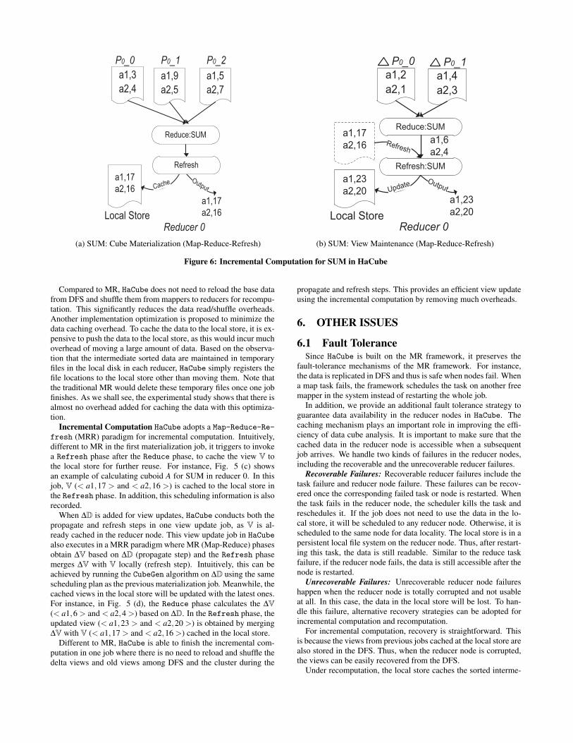
Figure 6: Incremental Computation for SUM in HaCube

Compared to MR, HaCube does not need to reload the base datafrom DFS and shuffle them from mappers to reducers for recompu-tation. This significantly reduces the data read/shuffle overheads.Another implementation optimization is proposed to minimize thedata caching overhead. To cache the data to the local store, it is ex-pensive to push the data to the local store, as this would incur muchoverhead of moving a large amount of data. Based on the observa-tion that the intermediate sorted data are maintained in temporaryfiles in the local disk in each reducer, HaCube simply registers thefile locations to the local store other than moving them. Note thatthe traditional MR would delete these temporary files once one jobfinishes. As we shall see, the experimental study shows that there isalmost no overhead added for caching the data with this optimiza-tion.

Incremental Computation HaCube adopts a Map-Reduce-Re-fresh (MRR) paradigm for incremental computation. Intuitively,different to MR in the first materialization job, it triggers to invokea Refresh phase after the Reduce phase, to cache the view V tothe local store for further reuse. For instance, Fig. 5 (c) showsan example of calculating cuboid A for SUM in reducer 0. In thisjob, V (< a1,17 > and < a2,16 >) is cached to the local store inthe Refresh phase. In addition, this scheduling information is alsorecorded.

When ∆D is added for view updates, HaCube conducts both thepropagate and refresh steps in one view update job, as V is al-ready cached in the reducer node. This view update job in HaCube

also executes in a MRR paradigm where MR (Map-Reduce) phasesobtain ∆V based on ∆D (propagate step) and the Refresh phasemerges ∆V with V locally (refresh step). Intuitively, this can beachieved by running the CubeGen algorithm on ∆D using the samescheduling plan as the previous materialization job. Meanwhile, thecached views in the local store will be updated with the latest ones.For instance, in Fig. 5 (d), the Reduce phase calculates the ∆V(< a1,6 > and < a2,4 >) based on ∆D. In the Refresh phase, theupdated view (< a1,23 > and < a2,20 >) is obtained by merging∆V with V (< a1,17 > and < a2,16 >) cached in the local store.

Different to MR, HaCube is able to finish the incremental com-putation in one job where there is no need to reload and shuffle thedelta views and old views among DFS and the cluster during the

propagate and refresh steps. This provides an efficient view updateusing the incremental computation by removing much overheads.

6. OTHER ISSUES

6.1 Fault ToleranceSince HaCube is built on the MR framework, it preserves the

fault-tolerance mechanisms of the MR framework. For instance,the data is replicated in DFS and thus is safe when nodes fail. Whena map task fails, the framework schedules the task on another freemapper in the system instead of restarting the whole job.

In addition, we provide an additional fault tolerance strategy toguarantee data availability in the reducer nodes in HaCube. Thecaching mechanism plays an important role in improving the effi-ciency of data cube analysis. It is important to make sure that thecached data in the reducer node is accessible when a subsequentjob arrives. We handle two kinds of failures in the reducer nodes,including the recoverable and the unrecoverable reducer failures.

Recoverable Failures: Recoverable reducer failures include thetask failure and reducer node failure. These failures can be recov-ered once the corresponding failed task or node is restarted. Whenthe task fails in the reducer node, the scheduler kills the task andreschedules it. If the job does not need to use the data in the lo-cal store, it will be scheduled to any reducer node. Otherwise, it isscheduled to the same node for data locality. The local store is in apersistent local file system on the reducer node. Thus, after restart-ing this task, the data is still readable. Similar to the reduce taskfailure, if the reducer node fails, the data is still accessible after thenode is restarted.

Unrecoverable Failures: Unrecoverable reducer node failureshappen when the reducer node is totally corrupted and not usableat all. In this case, the data in the local store will be lost. To han-dle this failure, alternative recovery strategies can be adopted forincremental computation and recomputation.

For incremental computation, recovery is straightforward. Thisis because the views from previous jobs cached at the local store arealso stored in the DFS. Thus, when the reducer node is corrupted,the views can be easily recovered from the DFS.

Under recomputation, the local store caches the sorted interme-

200

400

600

800

1000

1200

1400

1600

1800

600M 1.2B 1.8B 2.4B

Exe

cutio

n Ti

me(

s)

Data Size(Number of Tuples)

MulR_MulSSingR_MulSCubeGen_CacheCubeGen_NoCache

(a) MEDIAN

200

400

600

800

1000

1200

1400

1600

1800

600M 1.2B 1.8B 2.4B

Exe

cutio

n Ti

me(

s)

Data Size(Number of Tuples)

MulR_MulSSingR_MulSCubeGen_CacheCubeGen_NoCache

(b) SUM

Figure 7: CubeGen Performance Evaluation for Cube Materialization

diate reduce input data from the merge phase. To handle node fail-ures, HaCube adopts a lazy checkpointing strategy - a snapshot ofthe local store is stored to the DFS periodically. For cube analysis,if we make a snapshot of the cached data after each view update,it provides the fastest recovery. This is to ensure that data can bedirectly recovered from the previous view update stage. However,it is costly to perform checkpointing for each update.

On the other hand, if no snapshots are taken, once a node fails,we have to recompute it from scratch which is also computationallyexpensive. Instead, we advocate an intermediate solution that takesa snapshot after every s view updates where s can be set by the usersaccording to the view update and computer failure frequencies intheir cluster. With such a lazy checkpointing scheme, if a failurehappens, the system can recover by using the most recent snapshotand the new delta data added after the last checkpointing. Thus,HaCube only needs to store the latest snapshot and the data afterthe snapshot instead of storing all the base data from the beginning.

6.2 Storage Cost DiscussionWe argue that HaCube’s storage costs are acceptable.

• First, even though HaCube needs to cache extra data in thelocal store, the base data can be deleted from the file systemwhen there is no need to maintain them for other purposes.The cached data in the local store is sufficient to facilitateview updates when new data are added.

• Second, we can also reduce the number of replicas stored inthe DFS accordingly. The data cached in the local store canessentially be viewed as one replicated dataset.

• Third, HaCube only needs to cache one copy of the datasetfor different measures in each computation model. Recallthat all the measures can be processed together. Thus, forall measures issuing recomputation, the cached sorted rawdata is able to serve all of them. For all measures issuingincremental computation, the cached view data can be storedtogether to reduce storage overhead. For instance, assumethat both SUM and MAX need to be calculated, we can storethese two views together in the format of <dimension at-tributes, SUM, MAX> instead of maintaining them indepen-dently.

7. PERFORMANCE EVALUATIONWe evaluate HaCube on the Longhorn Hadoop cluster in TACC

(Texas Advanced Computing Center) [2]. Each node consists of 2

Intel Nehalem quad-core processors (8 cores) and 48GB memory.By default, the number of nodes used is 35 (and 280 cores).

We perform our studies on the classical dataset generated byTPC-D benchmark generators [3]. The TPC-D benchmark offersa rich environment representative of many decision support sys-tems. We study the cube views on the fact table, lineitem in thebenchmark. The attributes l_partkey, l_orderkey, l_suppkey andl_shipdate are used as the dimensions and the l_quantity as themeasure. We choose MEDIAN and SUM as the representativefunctions for evaluation. We report the result based on the aver-age execution time of three runs in each experiment.

7.1 Cube Materialization EvaluationBaseline Algorithms To study the benefit of the optimizations

adopted in CubeGen, we design two corresponding baseline al-gorithms to study each of them including MulR_MulS (computeeach cuboid using one MR job) and SingR_MulS (compute allthe cuboids using one MR job without batching them), which arewidely used for cube computations in MR. MulR_MulS is used tostudy the benefit of removing multiple data read overheads. SingR_MulS is used to study the benefit of sharing the shuffle and com-putation through batch processing.

In the following set of experiments, we vary the data size from600M (Million) to 2.4B (Billion) tuples.We study two versions ofthe CubeGen algorithm where CubeGen _Cache caches the dataand CubeGen_NoCache does not. This provides insights into theoverhead of caching the data to the local store.

7.1.1 Efficiency EvaluationWe first evaluate the performance improvement of CubeGen for

cube materialization. Fig. 7 (a) and (b) show the execution timeof all four algorithms for MEDIAN and SUM respectively. Asexpected, for both MEDIAN and SUM, our CubeGen-based algo-rithms are 2.2X and 1.6X faster than MulR_MulS and SingR_MulS

on average respectively. This indicates that computing the entirecube in one MR job reduces the overheads significantly comparedto the case where multiple MR jobs were issued which requiresreading data multiple times. In addition, it also demonstrates thatbatch processing highly reduces the size of intermediate data whichcan consequently minimize the overheads of data sorting, shufflingas well as computing.

7.1.2 Impact of Caching DataFigure 7 (a) and (b) also depict the impact of caching data. For

MEDIAN, we can see that the execution time of the CubeGen_Cachealgorithm is almost the same as CubeGen_NoCache as shown inFig. 7 (a). This confirms that our optimization to cache the data

through file registration instead of actual data movement does notcause much overhead. For SUM, we observe that CubeGen_Cacheperforms worse than CubeGen_NoCache. This is not surprisingas the former needs to write an extra view to the local file sys-tem. However, even though CubeGen_Cache incurs around 16%overhead to cache the view, as we will see later, it is superior toCubeGen_NoCache when it comes to view updates.

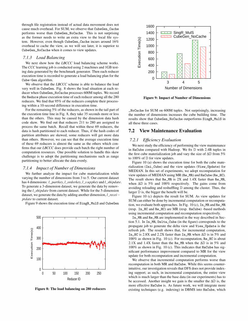
7.1.3 Load BalancingWe next show how the LBCCC load balancing scheme works.

The CCC learning job is conducted using 2 machines and 1GB test-ing data generated by the benchmark generator. Then each reducerexecution time is recorded to generate a load balancing plan for theCube-Gen algorithm.

We observe that the LBCCC scheme is able to balance the loadvery well in CubeGen. Fig. 8 shows the load situation at each re-ducer when CubeGen_NoCache processes 600M tuples. We recordthe Reduce phase execution time of each reducer among all the 280reducers. We find that 95% of the reducers complete their process-ing within a 10-second difference in execution time.

For the remaining 5% of the reducers, as shown in the tail part ofthe execution time line in Fig. 8, they take 35 seconds more or lessthan the others. This may be caused by the dimension data hashcode skew. We find out that reducers 211 to 280 are assigned toprocess the same batch. Recall that within these 69 reducers, thedata is hash partitioned to each reducer. Thus, if the hash codes ofpartition attributes are skewed, some reducers will get more datathan others. However, we can see that the average execution timeof these 69 reducers is almost the same as the others which con-firms that our LBCCC does provide each batch the right number ofcomputation resources. One possible solution to handle this skewchallenge is to adopt the partitioning mechanisms such as rangepartitioning to better allocate the data evenly.

7.1.4 Impact of Number of DimensionsWe further analyze the impact for cube materialization while

varying the number of dimensions from 3 to 5. Our current datasethas 4 dimensions: l_partkey, l_orderkey, l_s uppkey and l_shipdate.To generate a 3-dimension dataset, we generate the data by remov-ing the l_shipdate from current dataset. While for the 5-dimensiondataset, we generate the data by adding another dimension, l_recei−ptdate to current dataset.

Figure 9 shows the execution time of SingR_MulS and CubeGen

0

100

200

300

400

500

0 50 100 150 200 250

Execution T

ime(s

)

Reducer ID

Figure 8: The load balancing on 280 reducers

0

200

400

600

800

1000

1200

1400

1600

3 4 5

Exe

cutio

n T

ime(s

)

Number of Dimensions

SingR_MulSCubeGen_NoCache

Figure 9: Impact of Number of Dimensions

_NoCache for SUM on 600M tuples. Not surprisingly, increasingthe number of dimensions increases the cube building time. Theresults show that CubeGen_NoCache outperforms SingR_MulS inall these three cases.

7.2 View Maintenance Evaluation

7.2.1 Efficiency EvaluationWe next study the efficiency of performing the view maintenance

in HaCube compared with Hadoop. We fix D with 2.4B tuples inthe first cube materialization job and vary the size of ∆D from 5%to 100% of D for view updates.

Figure 10 (a) shows the execution time for both the cube mate-rialization (Ini_Cube) and the view updates (View_Update) forMEDIAN. In this set of experiments, we adopt recomputation forview updates of MEDIAN using MR (Re_MR) and HaCube (Re_HC).The result shows that Re_MR is 2X and 1.4X faster than Re_MR,when ∆D is 5% and 100% respectively. The gains come fromavoiding reloading and reshuffling D among the cluster. Thus, thelarger D is, the bigger the benefit will be.

Figure 10 (c) depicts the result for SUM. As view updates forSUM can either be done by incremental computation or recomputa-tion, we evaluate both approaches. In Fig. 10 (c), In_MR and Re_MR(resp. In_HC and Re_HC) are MR (resp. HaCube) -based methodsusing incremental computation and recomputation respectively.In_MR and Re_MR are implemented in the way described in Sec-

tion 5.1. In In_MR, Delta_Cube (in the figure) corresponds to thepropagate job to generate the delta view and View_Update is therefresh job. The result shows that, for incremental computation,In_HC is 2.8X and 2.2X faster than In_MR when ∆D is in 5% and100% as shown in Fig. 10 (c). For recomputation, Re_HC is about2.1X and 1.4X faster than the Re_MR when the ∆D is in 5% and100% as shown in Fig. 10 (c). This indicates that HaCube has sig-nificant performance improvement compared to MR for the viewupdate for both recomputation and incremental computation.

We observe that incremental computation performs worse thanrecomputation in both MR and HaCube. While this seems counter-intuitive, our investigation reveals that DFS does not provide index-ing support; as such, in incremental computation, the entire viewwhich is much larger than the base data (in our experiments) has tobe accessed. Another insight we gain is the smaller the ∆D is, themore effective HaCube is. As future work, we will integrate moreexisting techniques (e.g. indexing) in DBMS into HaCube, which

0

200

400

600

800

1000

1200

1400

1600

1800

Re_MR

Re_HC

Re_MR

Re_HC

Re_MR

Re_HC

Re_MR

Re_HC

Re_MR

Re_HC

Exe

cu

tio

n T

ime

(s)

Ini_CubeView_Update

100%50%20%10%5%

(a) Maintenance: MEDIAN

0

200

400

600

800

1000

1200

1400

1600

10 20 30 40

Exe

cutio

n T

ime(s

)

Number of Nodes

Ini_CubeView_Update

(b) Parallelism: MEDIAN

0

500

1000

1500

2000

2500

3000

3500

In_MR

In_HC

Re_MR

Re_HC

In_MR

In_HC

Re_MR

Re_HC

In_MR

In_HC

Re_MR

Re_HC

In_MR

In_HC

Re_MR

Re_HC

In_MR

In_HC

Re_MR

Re_HC

Execution T

ime(s

)

Ini_CubeDelta_CubeView_Update

100%50%20%10%5%

(c) Maintenance: SUM

0 200 400 600 800

1000 1200 1400 1600 1800 2000

10 20 30 40

Exe

cutio

n T

ime

(s)

Number of Nodes

Ini_CubeView_Update

(d) Parallelism: SUM

Figure 10: CubeGen Performance Evaluation for View Maintenance and Impact of Parallelism

will further improve the view update performance.

7.2.2 Impact of ParallelismWe further analyze the impact of parallelism on HaCube for both

cube materialization and view update while varying the number ofnodes from 10 to 40. The experiments use D with 600M tuples and∆D in 20% of D .

Figures 10 (b) and (d) report the execution time for MEDIANand SUM. Note that, in this experiment, incremental computationis used for SUM. We observe that for both recomputation and in-cremental computation, HaCube scales linearly on the testing dataset from 10 to 20 nodes, where the execution time almost reducesto half when the resources are doubled. From 20 nodes to 40 nodes,the benefit of parallelism decreases a little bit. This is reasonable,since the entire overheads include two parts, the setup of the frame-work and the cube computation; the former one may reduce thebenefits of increasing the computation resources while cube com-putation cost is not big enough.

8. RELATED WORKMuch research has been devoted to the problem of data cube

analysis [13]. A lot of studies have investigated efficient cube ma-terialization [28][27][4][31] and view maintenance [16][21]. Threeclassic cube computation approaches (Top-down [31] , Bottom-Up[4] and Hybrid [27]) have been well studied to share computationamong the lattice in a centralized system or a small cluster envi-ronment. Different to these approaches, CubeGen adopts a newstrategy to partition and batch the cuboids according to their prefix

order to tackle the new challenges brought by MR. It utilizes thesorting feature better in MR-like systems such that no extra sortingneeded during materialization.

Existing works [23] [29] have adopted MR to build closed cubesfor algebraic measures. However, both of these works do not pro-vide a generic algorithm that can balance the load to materializethe cube for different measures. Nandi et al. [19] provided a solu-tion to a special case during the cube computation under MR whereone reducer gets the “hot spot” group-by cell with a large numberof tuples. This complements our work and can be employed tohandle such a case when one reducer is overloaded. We note thatHaCube is able to support all these existing cube materializationalgorithms. Last but not the least, none of these aforementionedworks have developed any techniques for view maintenance. Thisis, to the best of our knowledge, the first work to address the datacube view maintenance in MR-like systems.

Our work is also related to the problem of incremental computa-tions. Existing works [5][14][15] have studied some techniques forincremental computations for single operators in MR. HaLoop [6]is designed to support iterative operations through a similar cachingmechanism which is used for different purposes under a differentapplication context. Restore [10] also shares the similar spirit tokeep the intermediate results (either the output of one MR job or thedata operated within one job) to DFS in a workflow and reuse themin the future. For data cube computation, as the size of intermediateresults is large, HaCube adopts a different data caching mechanismto guarantee the data locality that the cached data can be directlyused from local store. This avoids the overhead incurred by Restore

in reloading and reshuffling data from DFS. Furthermore, none ofthese existing works provide explicit support and techniques fordata cube analysis under OLAP and data warehousing semantics.

9. CONCLUSIONIt is of critical importance to develop new scalable and efficient

data cube analysis systems on a big cluster with low-cost commod-ity machines to face the challenges brought by the large-scale ofdata, to provide a better query response and decision making sup-port. In this paper, we made one step towards developing sucha system, HaCube an extension of MapReduce, by integrating thegood features from both MapReduce (e.g. Scalability) and par-allel DBMS (e.g. Local Store). We showed how to batch andshare the computations to salvage partial work done by facilitat-ing the features in MapReduce-like systems towards an efficientcube materialization. We also proposed one load balancing strategysuch that the load in each reducer can be balanced. Furthermore,we demonstrated how HaCube supports an efficient view mainte-nance by facilitating the extension leveraging a new computationparadigm. The experimental results showed that our proposed cubematerialization approach is at least 1.6X to 2.2X faster than thenaive algorithms and HaCube performs at least 2.2X to 2.8X fasterthan Hadoop for view maintenance. We expect HaCube to fur-ther improve the performance by integrating more techniques fromDBMS, such as indexing techniques.

10. REFERENCES[1] Hadoop. http://hadoop.apache.org/.[2] Tacc longhorn cluster. https://www.tacc.utexas.edu/.[3] Tpc-h , ad-hoc, decision support benchmark. Available at:

www.tpc.org/tpch/.[4] Kevin S. Beyer and Raghu Ramakrishnan. Bottom-up

computation of sparse and iceberg cubes. In SIGMOD, pages359–370, 1999.

[5] P. Bhatotia, A. Wieder, R. Rodrigues, U. A. Acar, andR. Pasquini. Incoop: Mapreduce for incrementalcomputations. In SOCC, 2011.

[6] Yingyi Bu, Bill Howe, Magdalena Balazinska, andMichael D. Ernst. Haloop: Efficient iterative data processingon large clusters. PVLDB, 3(1):285–296, 2010.

[7] Edward Y. Chang, Hongjie Bai, and Kaihua Zhu. Parallelalgorithms for mining large-scale rich-media data. In ACMMultimedia, pages 917–918, 2009.

[8] Cheng-Tao Chu, Sang Kyun Kim, Yi-An Lin, YuanYuan Yu,Gary R. Bradski, Andrew Y. Ng, and Kunle Olukotun.Map-reduce for machine learning on multicore. In NIPS,pages 281–288, 2006.

[9] Jeffrey Dean and Sanjay Ghemawat. Mapreduce: Simplifieddata processing on large clusters. In OSDI, pages 137–150,2004.

[10] Iman Elghandour and Ashraf Aboulnaga. Restore: Reusingresults of mapreduce jobs. PVLDB, 5(6):586–597, 2012.

[11] Rainer Gemulla. Sampling algorithms for evolving datasets.PhD thesis, 2008.

[12] Dan Gillick, Arlo Faria, and John Denero. Mapreduce:Distributed computing for machine learning, 2006.

[13] Jim Gray, A. Bosworth, A. Layman, and D. Reichart. Datacube: A relational aggregation operator generalizinggroup-by cross-tab and sub-totals. In ICDE, pages 152–159,1996.

[14] Thomas Jörg, Roya Parvizi, Hu Yong, and Stefan Dessloch.Incremental recomputations in mapreduce. In CloudDB,pages 7–14, 2011.

[15] R. Lämmel and D. Saile. Mapreduce with deltas. In PDPTA,2011.

[16] Ki Yong Lee and Myoung Ho Kim. Efficient incrementalmaintenance of data cubes. In VLDB, pages 823–833, 2006.

[17] J. Lin and C. Dyer. Data-intensive text processing withmapreduce. Synthesis Lectures on Human LanguageTechnologies, 3(1):1–177, 2010.

[18] I. S. Mumick, D. Quass, and B. S. Mumick. Maintenace ofdata cubes and summary tables in a warehouse. In SIGMOD,pages 100–111, 1997.

[19] Arnab Nandi, Cong Yu, Philip Bohannon, and RaghuRamakrishnan. Distributed cube materialization on holisticmeasures. In ICDE, pages 183–194, 2011.

[20] Raymond T. Ng, Alan S. Wagner, and Yu Yin. Iceberg-cubecomputation with pc clusters. In SIGMOD, pages 25–36,2001.

[21] Themistoklis Palpanas, Richard Sidle, Roberta Cochrane,and Hamid Pirahesh. Incremental maintenance fornon-distributive aggregate functions. In VLDB, pages802–813, 2002.

[22] G. Sudha Sadasivam and G. Baktavatchalam. A novelapproach to multiple sequence alignment using hadoop datagrids. IJBRA, 6(5):472–483, 2010.

[23] Kuznecov Sergey and Kudryavcev Yury. Applyingmap-reduce paradigm for parallel closed cube computation.In DBKDA, pages 62–67, 2009.

[24] Zhengkui Wang, Divyakant Agrawal, and Kian-Lee Tan.Cosac: A framework for combinatorial statistical analysis oncloud. IEEE Transactions on Knowledge and DataEngineering, 25(9):2010–2023, 2013.

[25] Zhengkui Wang, Yue Wang, Kian-Lee Tan, Limsoon Wong,and Divyakant Agrawal. Ceo: A cloud epistasis computingmodel in gwas. In Proc. BIBM‘10, pages 85–90, 2010.

[26] Zhengkui Wang, Yue Wang, Kian-Lee Tan, Limsoon Wong,and Divyakant Agrawal. eceo: an efficient cloud epistasiscomputing model in genome-wide association study.Bioinformatics, 27(8):1045–1051, 2011.

[27] Dong Xin, Jiawei Han, Xiaolei Li, and Benjamin W. Wah.Computing iceberg cubes by top-down and bottom-upintegration: The starcubing approach. TKDE, 19(1):111–126,2007.

[28] Dong Xin, Jiawei Han, and Benjamin W. Wah. Star-cubing:Computing iceberg cubes by top-down and bottom-upintegration. In VLDB, pages 476–487, 2003.

[29] Jinguo You, Jianqing Xi, Pingjian Zhang, and Hu Chen. Aparallel algorithm for closed cube computation. InACIS-ICIS, pages 95–99, 2008.

[30] Weizhong Zhao, Huifang Ma, and Qing He. Parallel k-meansclustering based on mapreduce. In CloudCom, volume 5931of Lecture Notes in Computer Science, pages 674–679.Springer, 2009.

[31] Yihong Zhao, Prasad M. Deshpande, and Jeffrey F.Naughton. An array-based algorithm for simultaneousmultidimensional aggregates. In SIGMOD, pages 159–170,1997.