sat: algorithms and applicationsusers.rsise.anu.edu.au/~anbu/slides/aaai07/... · sat resources and...
TRANSCRIPT

SAT: Algorithms and Applications
Anbulagan and Jussi Rintanen
NICTA Ltd and the Australian National University (ANU)Canberra, Australia
Tutorial presentation at AAAI-07, Vancouver, Canada, July 22, 2007
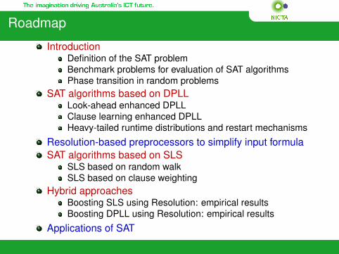
Roadmap
IntroductionDefinition of the SAT problemBenchmark problems for evaluation of SAT algorithmsPhase transition in random problems
SAT algorithms based on DPLLLook-ahead enhanced DPLLClause learning enhanced DPLLHeavy-tailed runtime distributions and restart mechanisms
Resolution-based preprocessors to simplify input formulaSAT algorithms based on SLS
SLS based on random walkSLS based on clause weighting
Hybrid approachesBoosting SLS using Resolution: empirical resultsBoosting DPLL using Resolution: empirical results
Applications of SAT

SAT Resources and Challenges
Benchmark Datawww.satlib.org
SAT Solverswww.satcompetition.orgAuthors website
International SAT Conference (10th in 2007)More information about SAT
Register to: www.satlive.orgChallenges
Ten Challenges in Propositional Reasoning and Search[Selman et al., 1997]Ten Challenges Redux: Recent Progress in PropositionalReasoning and Search [Kautz & Selman, 2003]

Problems – Traffic Management

Problems – Nurses Rostering
Many real-world problems can be expressed as a list ofconstraints.
Answer is an assignment to variables that satisfy all theconstraints.
Example:Scheduling nurses to work in shifts at a hospital
Some nurses do not work at nightNo one can work more than H hours a weekSome pairs of nurses cannot be on the same shiftIs there at least one assignment of nurses to shifts thatsatisfy all the constraints?
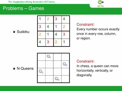
Problems – Games
Sudoku
Constraint:Every number occurs exactlyonce in every row, column,or region.
N-Queens
Constraint:In chess, a queen can movehorizontally, vertically, ordiagonally.

A Simple Problem: Student–Courses
A student would like to decide on which subjects he should takefor the next session. He has the following requirements:
He would like to take Math or drop BiologyHe would like to take Biology or AlgorithmsHe does not want to take Math and Algorithms together
Which subjects the student can take?
F = (X ∨ ¬Y ) ∧ (Y ∨ Z ) ∧ (¬X ∨ ¬Z )
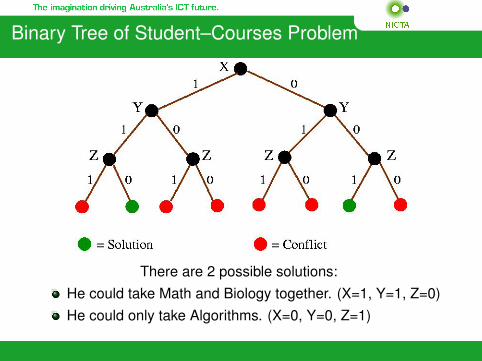
Binary Tree of Student–Courses Problem
There are 2 possible solutions:He could take Math and Biology together. (X=1, Y=1, Z=0)He could only take Algorithms. (X=0, Y=0, Z=1)

Practical Applications of SAT
AI Planning and Scheduling
Bioinformatics
Data Cleaning
Diagnosis
Electronic Design Automationand Verification
FPGA Routing
Games
Knowledge Discovery
Security: cryptographic keysearch
Theorem Proving
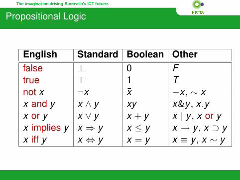
Propositional Logic
English Standard Boolean Otherfalse ⊥ 0 Ftrue > 1 Tnot x ¬x x −x , ∼ xx and y x ∧ y xy x&y , x .yx or y x ∨ y x + y x | y , x or yx implies y x ⇒ y x ≤ y x → y , x ⊃ yx iff y x ⇔ y x = y x ≡ y , x ∼ y
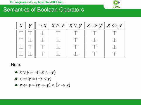
Semantics of Boolean Operators
x y ¬ x x ∧ y x ∨ y x ⇒ y x ⇔ y> > ⊥ > > > >> ⊥ ⊥ ⊥ > ⊥ ⊥⊥ > > ⊥ > > ⊥⊥ ⊥ > ⊥ ⊥ > >
Note:
x ∨ y = ¬(¬x ∧ ¬y)
x ⇒ y = (¬x ∨ y )x ⇔ y = (x ⇒ y ) ∧ (y ⇒ x)
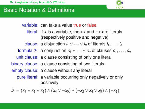
Basic Notation & Definitions
variable: can take a value true or false.literal: if x is a variable, then x and ¬x are literals
(respectively positive and negative)clause: a disjunction l1 ∨ · · · ∨ ln of literals l1, . . . , ln
formula F : a conjunction c1 ∧ · · · ∧ cn of clauses c1, . . . , cn
unit clause: a clause consisting of only one literalbinary clause: a clause consisting of two literalsempty clause: a clause without any literal
pure literal: a variable occurring only negatively or onlypositively
F = (x1 ∨ x2 ∨ x3) ∧ (x4 ∨ ¬x5) ∧ (¬x2 ∨ x4 ∨ x5) ∧ (¬x3)
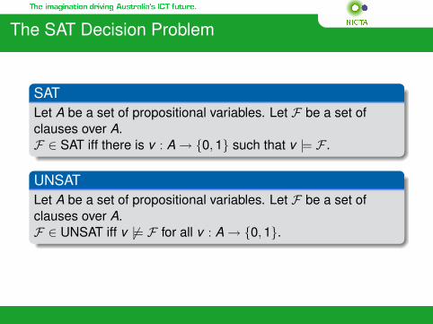
The SAT Decision Problem
SATLet A be a set of propositional variables. Let F be a set ofclauses over A.F ∈ SAT iff there is v : A → {0, 1} such that v |= F .
UNSATLet A be a set of propositional variables. Let F be a set ofclauses over A.F ∈ UNSAT iff v 6|= F for all v : A → {0, 1}.
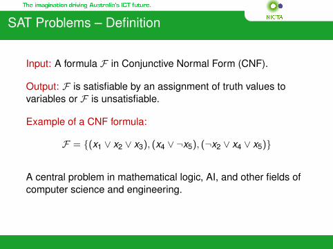
SAT Problems – Definition
Input: A formula F in Conjunctive Normal Form (CNF).
Output: F is satisfiable by an assignment of truth values tovariables or F is unsatisfiable.
Example of a CNF formula:
F = {(x1 ∨ x2 ∨ x3), (x4 ∨ ¬x5), (¬x2 ∨ x4 ∨ x5)}
A central problem in mathematical logic, AI, and other fields ofcomputer science and engineering.
Complexity Class NP
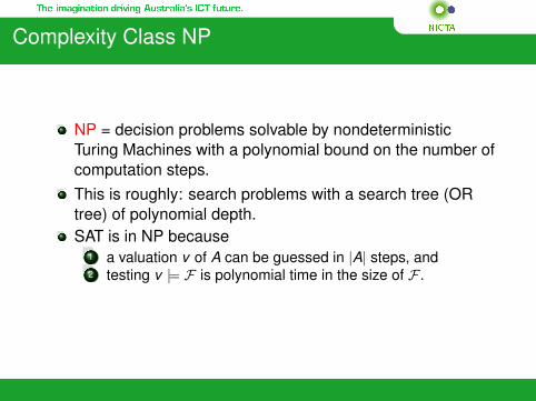
NP = decision problems solvable by nondeterministicTuring Machines with a polynomial bound on the number ofcomputation steps.This is roughly: search problems with a search tree (ORtree) of polynomial depth.SAT is in NP because
1 a valuation v of A can be guessed in |A| steps, and2 testing v |= F is polynomial time in the size of F .
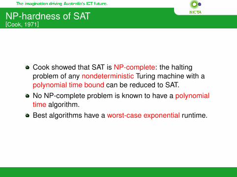
NP-hardness of SAT[Cook, 1971]
Cook showed that SAT is NP-complete: the haltingproblem of any nondeterministic Turing machine with apolynomial time bound can be reduced to SAT.No NP-complete problem is known to have a polynomialtime algorithm.Best algorithms have a worst-case exponential runtime.
SAT Benchmark Problems
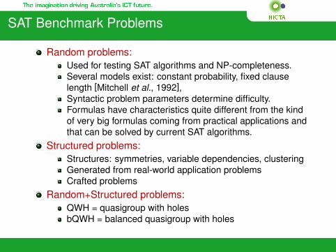
Random problems:Used for testing SAT algorithms and NP-completeness.Several models exist: constant probability, fixed clauselength [Mitchell et al., 1992],Syntactic problem parameters determine difficulty.Formulas have characteristics quite different from the kindof very big formulas coming from practical applications andthat can be solved by current SAT algorithms.
Structured problems:Structures: symmetries, variable dependencies, clusteringGenerated from real-world application problemsCrafted problems
Random+Structured problems:QWH = quasigroup with holesbQWH = balanced quasigroup with holes
Random ProblemsAn Example
c 1p cnf 64 254
-9 -31 -50 03 -32 -46 0
-26 -53 64 09 11 -27 0
-10 55 -59 0-21 -36 -51 039 -48 -53 027 -33 37 043 -58 -64 0
-12 21 -59 010 -27 -43 0
-15 -31 -62 01 -20 28 0
-9 -14 -64 0-5 37 53 0
-32 -37 49 0..........
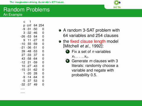
A random 3-SAT problem with64 variables and 254 clausesthe fixed clause length model[Mitchell et al., 1992]:
1 Fix a set of n variablesx1, . . . , xn.
2 Generate m clauses with 3literals: randomly choose avariable and negate withprobability 0.5.
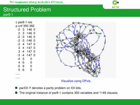
Structured Problempar8-1
c par8-1-resp cnf 350 382-2 3 146 02 3 -146 0
-2 -3 146 0-2 -3 -146 0-3 4 147 03 4 -147 03 -4 147 0
-3 -4 -147 0-4 5 04 -5 0
-5 6 05 -6 0
.....
.....Visualize using DPvis.
parXX-Y denotes a parity problem on XX bits.
The original instance of par8-1 contains 350 variables and 1149 clauses.
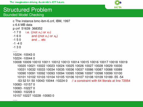
Structured ProblemBounded Model Checking
c The instance bmc-ibm-6.cnf, IBM, 1997c 6.6 MB datap cnf 51639 368352-1 7 0 i.e. ((not x1) or x7)-1 6 0 and ((not x1) or x6)-1 5 0 and ... etc-1 -4 0-1 3 0.....10224 -10043 010224 -10044 010008 10009 10010 10011 10012 10013 10014 10015 10016 10017 10018 10019
10020 10021 10022 10023 10024 10025 10026 10027 10028 10029 1003010031 10032 10033 10034 10035 10036 10037 10086 10087 10088 1008910090 10091 10092 10093 10094 10095 10096 10097 10098 10099 1010010101 10102 10103 10104 10105 10106 10107 10108 10109 10189 -55 -54-53 52 51 50 10043 10044 -10224 0 // a constraint with 64 literals at line 72054
10083 -10157 010083 -10227 010083 -10228 010157 10227 10228 -10083 0.....
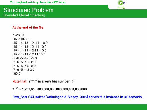
Structured ProblemBounded Model Checking
At the end of the file
7 -260 01072 1070 0-15 -14 -13 -12 -11 -10 0-15 -14 -13 -12 -11 10 0-15 -14 -13 -12 11 -10 0-15 -14 -13 -12 11 10 0-7 -6 -5 -4 -3 -2 0-7 -6 -5 -4 -3 2 0-7 -6 -5 -4 3 -2 0-7 -6 -5 -4 3 2 0185 0
Note that: 251639 is a very big number !!!
2100 = 1,267,650,000,000,000,000,000,000,000,000
Dew_Satz SAT solver [Anbulagan & Slaney, 2005] solves this instance in 36 seconds.
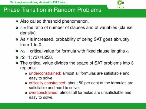
Phase Transition in Random Problems
Also called threshold phenomenon.r = the ratio of number of clauses and of variables (clausedensity).As r is increased, probability of being SAT goes abruptlyfrom 1 to 0.rα = critical value for formula with fixed clause lengths α
r2=1; r3u4.258.The critical value divides the space of SAT problems into 3regions:
underconstrained: almost all formulas are satisfiable andeasy to solve;critically constrained: about 50 per cent of the formulas aresatisfiable and hard to solve;overconstrained: almost all formulas are unsatisfiable andeasy to solve.
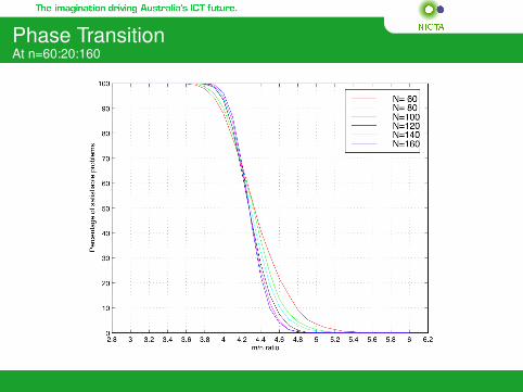
Phase TransitionAt n=60:20:160

Phase Transition and Difficulty LevelAt n=200
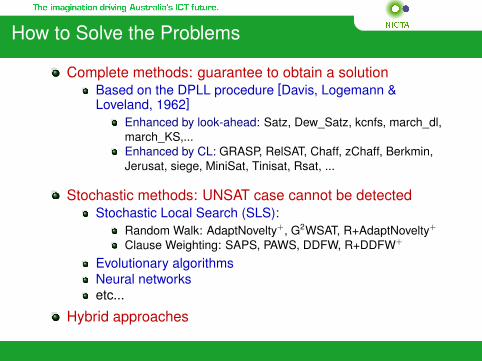
How to Solve the Problems
Complete methods: guarantee to obtain a solutionBased on the DPLL procedure [Davis, Logemann &Loveland, 1962]
Enhanced by look-ahead: Satz, Dew_Satz, kcnfs, march_dl,march_KS,...Enhanced by CL: GRASP, RelSAT, Chaff, zChaff, Berkmin,Jerusat, siege, MiniSat, Tinisat, Rsat, ...
Stochastic methods: UNSAT case cannot be detectedStochastic Local Search (SLS):
Random Walk: AdaptNovelty+, G2WSAT, R+AdaptNovelty+
Clause Weighting: SAPS, PAWS, DDFW, R+DDFW+
Evolutionary algorithmsNeural networksetc...
Hybrid approaches
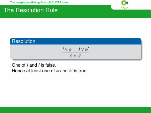
The Resolution Rule
Resolution
l ∨ φ l ∨ φ′
φ ∨ φ′
One of l and l is false.Hence at least one of φ and φ′ is true.
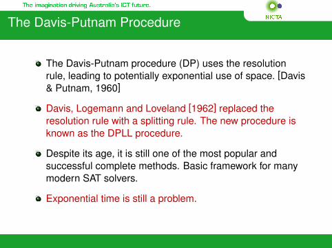
The Davis-Putnam Procedure
The Davis-Putnam procedure (DP) uses the resolutionrule, leading to potentially exponential use of space. [Davis& Putnam, 1960]
Davis, Logemann and Loveland [1962] replaced theresolution rule with a splitting rule. The new procedure isknown as the DPLL procedure.
Despite its age, it is still one of the most popular andsuccessful complete methods. Basic framework for manymodern SAT solvers.
Exponential time is still a problem.
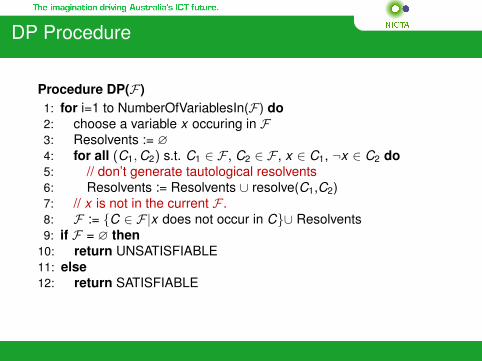
DP Procedure
Procedure DP(F)1: for i=1 to NumberOfVariablesIn(F) do2: choose a variable x occuring in F3: Resolvents := ∅4: for all (C1, C2) s.t. C1 ∈ F , C2 ∈ F , x ∈ C1, ¬x ∈ C2 do5: // don’t generate tautological resolvents6: Resolvents := Resolvents ∪ resolve(C1,C2)7: // x is not in the current F .8: F := {C ∈ F|x does not occur in C}∪ Resolvents9: if F = ∅ then
10: return UNSATISFIABLE11: else12: return SATISFIABLE
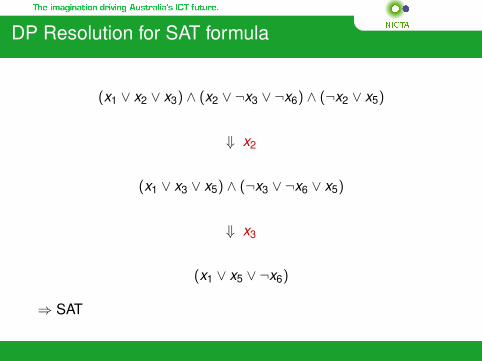
DP Resolution for SAT formula
(x1 ∨ x2 ∨ x3) ∧ (x2 ∨ ¬x3 ∨ ¬x6) ∧ (¬x2 ∨ x5)
⇓ x2
(x1 ∨ x3 ∨ x5) ∧ (¬x3 ∨ ¬x6 ∨ x5)
⇓ x3
(x1 ∨ x5 ∨ ¬x6)
⇒ SAT
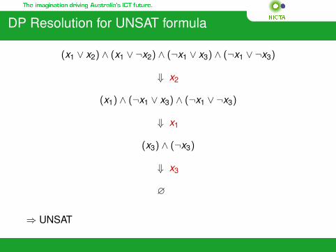
DP Resolution for UNSAT formula
(x1 ∨ x2) ∧ (x1 ∨ ¬x2) ∧ (¬x1 ∨ x3) ∧ (¬x1 ∨ ¬x3)
⇓ x2
(x1) ∧ (¬x1 ∨ x3) ∧ (¬x1 ∨ ¬x3)
⇓ x1
(x3) ∧ (¬x3)
⇓ x3
∅
⇒ UNSAT
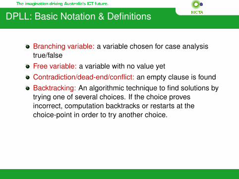
DPLL: Basic Notation & Definitions
Branching variable: a variable chosen for case analysistrue/falseFree variable: a variable with no value yetContradiction/dead-end/conflict: an empty clause is foundBacktracking: An algorithmic technique to find solutions bytrying one of several choices. If the choice provesincorrect, computation backtracks or restarts at thechoice-point in order to try another choice.
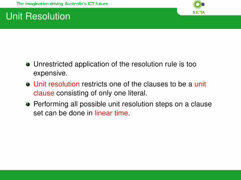
Unit Resolution
Unrestricted application of the resolution rule is tooexpensive.Unit resolution restricts one of the clauses to be a unitclause consisting of only one literal.Performing all possible unit resolution steps on a clauseset can be done in linear time.
Unit Propagation
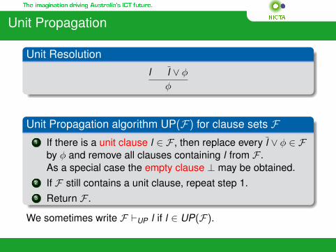
Unit Resolution
l l ∨ φ
φ
Unit Propagation algorithm UP(F) for clause sets F1 If there is a unit clause l ∈ F , then replace every l ∨ φ ∈ F
by φ and remove all clauses containing l from F .As a special case the empty clause ⊥ may be obtained.
2 If F still contains a unit clause, repeat step 1.3 Return F .
We sometimes write F `UP l if l ∈ UP(F).
The DPLL Procedure
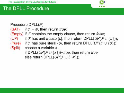
Procedure DPLL(F)(SAT) if F = ∅, then return true;(Empty) if F contains the empty clause, then return false;(UP) if F has unit clause {u}, then return DPLL(UP(F ∪ {u}));(Pure) if F has pure literal {p}, then return DPLL(UP(F ∪ {p}));(Split) choose a variable x ;
if DPLL(UP(F ∪ {x}))=true, then return trueelse return DPLL(UP(F ∪ {¬x}));
Search Tree of the DPLL Procedure
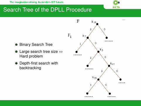
Binary Search Tree
Large search tree size ⇔Hard problem
Depth-first search withbacktracking
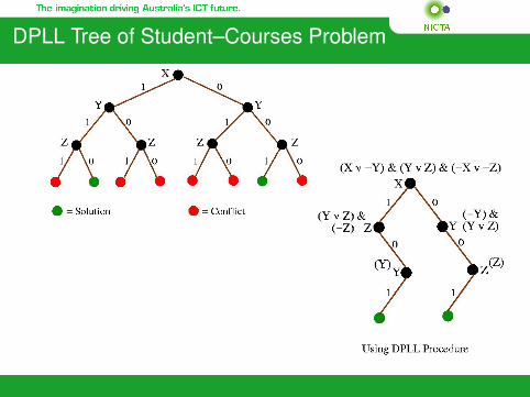
DPLL Tree of Student–Courses Problem
DPLL Performance: Original vs Variants
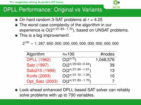
On hard random 3-SAT problems at r = 4.25The worst case complexity of the algorithm in ourexperience is O(2n/21.83−1.70), based on UNSAT problems.This is a big improvement!
2100 = 1, 267, 650, 000, 000, 000, 000, 000, 000, 000, 000
Algorithm n=100 #nodesDPLL (1962) O(2n/5) 1,048,576Satz (1997) O(2n/20.63+0.44) 39Satz215 (1999) O(2n/21.04−1.01) 13Kcnfs (2003) O(2n/21.10−1.35) 10Opt_Satz (2003) O(2n/21.83−1.70) 7
Look-ahead enhanced DPLL based SAT solver can reliablysolve problems with up to 700 variables.
Heuristics for the DPLL Procedure
Objective: to reduce search tree size by choosing a bestbranching variable at each node of the search tree.
Central issue:how to select the next best branchingvariable?

Branching Heuristics for DPLL Procedure
SimpleUse simple heuristics for branching variables selectionBased on counting occurrences of literals or variables
SophisticatedUse sophisticated heuristics for branching variablesselectionNeed more resources and efforts
Simple Branching Heuristics
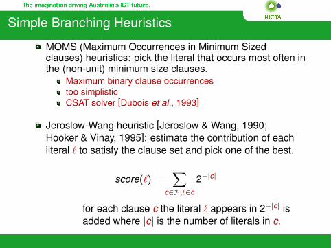
MOMS (Maximum Occurrences in Minimum Sizedclauses) heuristics: pick the literal that occurs most often inthe (non-unit) minimum size clauses.
Maximum binary clause occurrencestoo simplisticCSAT solver [Dubois et al., 1993]
Jeroslow-Wang heuristic [Jeroslow & Wang, 1990;Hooker & Vinay, 1995]: estimate the contribution of eachliteral ` to satisfy the clause set and pick one of the best.
score(`) =∑
c∈F ,`∈c
2−|c|
for each clause c the literal ` appears in 2−|c| isadded where |c| is the number of literals in c.

Algorithms for SAT Solving
Look-ahead based DPLL
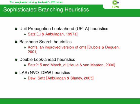
Sophisticated Branching Heuristics
Unit Propagation Look-ahead (UPLA) heuristicsSatz [Li & Anbulagan, 1997a]
Backbone Search heuristicsKcnfs, an improved version of cnfs [Dubois & Dequen,2001]
Double Look-ahead heuristicsSatz215 and March_dl [Heule & van Maaren, 2006]
LAS+NVO+DEW heuristicsDew_Satz [Anbulagan & Slaney, 2005]
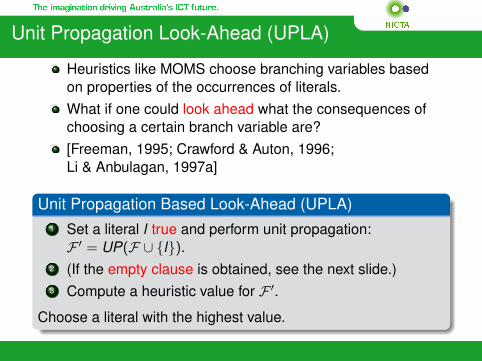
Unit Propagation Look-Ahead (UPLA)
Heuristics like MOMS choose branching variables basedon properties of the occurrences of literals.What if one could look ahead what the consequences ofchoosing a certain branch variable are?[Freeman, 1995; Crawford & Auton, 1996;Li & Anbulagan, 1997a]
Unit Propagation Based Look-Ahead (UPLA)1 Set a literal l true and perform unit propagation:F ′ = UP(F ∪ {l}).
2 (If the empty clause is obtained, see the next slide.)3 Compute a heuristic value for F ′.
Choose a literal with the highest value.
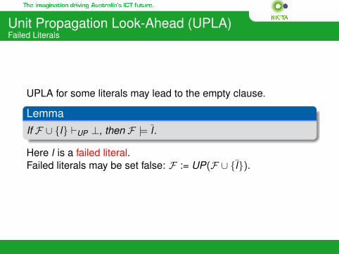
Unit Propagation Look-Ahead (UPLA)Failed Literals
UPLA for some literals may lead to the empty clause.
LemmaIf F ∪ {l} `UP ⊥, then F |= l .
Here l is a failed literal.Failed literals may be set false: F := UP(F ∪ {l}).
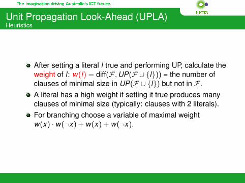
Unit Propagation Look-Ahead (UPLA)Heuristics
After setting a literal l true and performing UP, calculate theweight of l : w(l) = diff(F , UP(F ∪ {l})) = the number ofclauses of minimal size in UP(F ∪ {l}) but not in F .A literal has a high weight if setting it true produces manyclauses of minimal size (typically: clauses with 2 literals).For branching choose a variable of maximal weightw(x) · w(¬x) + w(x) + w(¬x).
Unit Propagation Look-Ahead (UPLA)Restricted UPLA
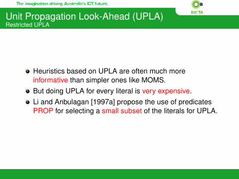
Heuristics based on UPLA are often much moreinformative than simpler ones like MOMS.But doing UPLA for every literal is very expensive.Li and Anbulagan [1997a] propose the use of predicatesPROP for selecting a small subset of the literals for UPLA.
Unit Propagation Look-Ahead (UPLA)The Predicate PROP in the Satz solver
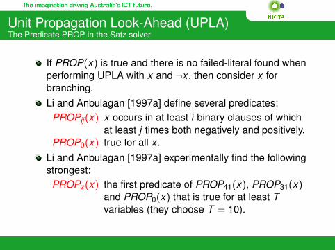
If PROP(x) is true and there is no failed-literal found whenperforming UPLA with x and ¬x , then consider x forbranching.Li and Anbulagan [1997a] define several predicates:
PROPij(x) x occurs in at least i binary clauses of whichat least j times both negatively and positively.
PROP0(x) true for all x .Li and Anbulagan [1997a] experimentally find the followingstrongest:PROPz(x) the first predicate of PROP41(x), PROP31(x)
and PROP0(x) that is true for at least Tvariables (they choose T = 10).
Dew_Satz: LAS+NVO+DEW Heuristics[Anbulagan & Slaney, 2005]
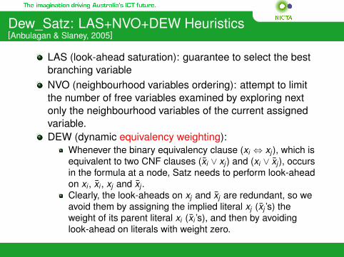
LAS (look-ahead saturation): guarantee to select the bestbranching variableNVO (neighbourhood variables ordering): attempt to limitthe number of free variables examined by exploring nextonly the neighbourhood variables of the current assignedvariable.DEW (dynamic equivalency weighting):
Whenever the binary equivalency clause (xi ⇔ xj ), which isequivalent to two CNF clauses (xi ∨ xj ) and (xi ∨ xj ), occursin the formula at a node, Satz needs to perform look-aheadon xi , xi , xj and xj .Clearly, the look-aheads on xj and xj are redundant, so weavoid them by assigning the implied literal xj (xj ’s) theweight of its parent literal xi (xi ’s), and then by avoidinglook-ahead on literals with weight zero.
EqSatz
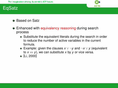
Based on Satz
Enhanced with equivalency reasoning during searchprocess
Substitute the equivalent literals during the search in orderto reduce the number of active variables in the currentformula.Example: given the clauses x ∨ ¬y and ¬x ∨ y (equivalentto x ⇔ y ), we can substitute x by y or vice versa.[Li, 2000]
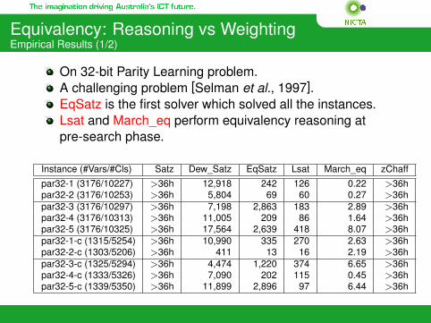
Equivalency: Reasoning vs WeightingEmpirical Results (1/2)
On 32-bit Parity Learning problem.A challenging problem [Selman et al., 1997].EqSatz is the first solver which solved all the instances.Lsat and March_eq perform equivalency reasoning atpre-search phase.
Instance (#Vars/#Cls) Satz Dew_Satz EqSatz Lsat March_eq zChaffpar32-1 (3176/10227) >36h 12,918 242 126 0.22 >36hpar32-2 (3176/10253) >36h 5,804 69 60 0.27 >36hpar32-3 (3176/10297) >36h 7,198 2,863 183 2.89 >36hpar32-4 (3176/10313) >36h 11,005 209 86 1.64 >36hpar32-5 (3176/10325) >36h 17,564 2,639 418 8.07 >36hpar32-1-c (1315/5254) >36h 10,990 335 270 2.63 >36hpar32-2-c (1303/5206) >36h 411 13 16 2.19 >36hpar32-3-c (1325/5294) >36h 4,474 1,220 374 6.65 >36hpar32-4-c (1333/5326) >36h 7,090 202 115 0.45 >36hpar32-5-c (1339/5350) >36h 11,899 2,896 97 6.44 >36h
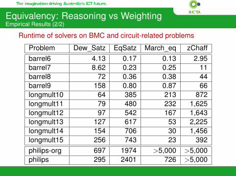
Equivalency: Reasoning vs WeightingEmpirical Results (2/2)
Runtime of solvers on BMC and circuit-related problems
Problem Dew_Satz EqSatz March_eq zChaffbarrel6 4.13 0.17 0.13 2.95barrel7 8.62 0.23 0.25 11barrel8 72 0.36 0.38 44barrel9 158 0.80 0.87 66longmult10 64 385 213 872longmult11 79 480 232 1,625longmult12 97 542 167 1,643longmult13 127 617 53 2,225longmult14 154 706 30 1,456longmult15 256 743 23 392philips-org 697 1974 >5,000 >5,000philips 295 2401 726 >5,000

Algorithms for SAT Solving
Clause learning (CL) based DPLL
DPLL with backjumping
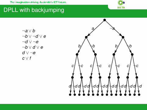
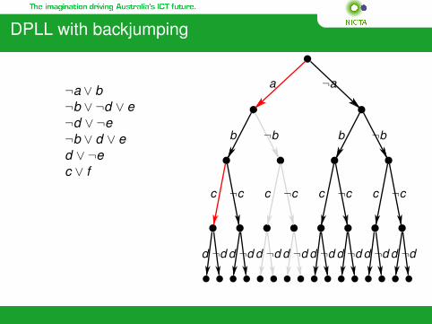
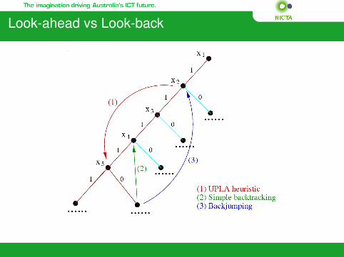
The DPLL backtracking procedure often discovers thesame conflicts repeatedly.In a branch l1, l2, . . . , ln−1, ln, after ln and ln have led toconflicts (derivation of ⊥), ln−1 is always tried next, evenwhen it is irrelevant to the conflicts with ln and ln.Backjumping (Gaschnig, 1979) can be adapted to DPLL tobacktrack from ln to li when li+1, . . . , ln−1 are all irrelevant.
DPLL with backjumping
¬a ∨ b¬b ∨ ¬d ∨ e¬d ∨ ¬e¬b ∨ d ∨ ed ∨ ¬ec ∨ f
¬aa
¬bb¬bb
¬cc¬cc ¬cc¬cc
¬dd¬dd¬dd¬dd ¬dd¬dd¬dd¬dd

DPLL with backjumping
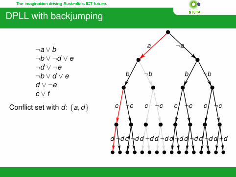
¬a ∨ b¬b ∨ ¬d ∨ e¬d ∨ ¬e¬b ∨ d ∨ ed ∨ ¬ec ∨ f
¬aa
¬bb¬bb
¬cc¬cc ¬cc¬cc
¬dd¬dd¬dd¬dd ¬dd¬dd¬dd¬dd
DPLL with backjumping
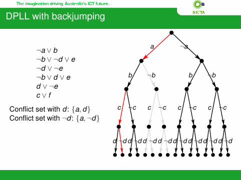
¬a ∨ b¬b ∨ ¬d ∨ e¬d ∨ ¬e¬b ∨ d ∨ ed ∨ ¬ec ∨ f
¬aa
¬bb¬bb
¬cc¬cc ¬cc¬cc
¬dd¬dd¬dd¬dd ¬dd¬dd¬dd¬dd
DPLL with backjumping
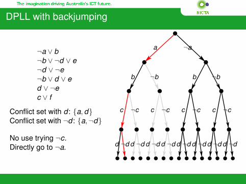
¬a ∨ b¬b ∨ ¬d ∨ e¬d ∨ ¬e¬b ∨ d ∨ ed ∨ ¬ec ∨ f
Conflict set with d : {a, d}
¬aa
¬bb¬bb
¬cc¬cc ¬cc¬cc
¬dd¬dd¬dd¬dd ¬dd¬dd¬dd¬dd
DPLL with backjumping
¬a ∨ b¬b ∨ ¬d ∨ e¬d ∨ ¬e¬b ∨ d ∨ ed ∨ ¬ec ∨ f
Conflict set with d : {a, d}Conflict set with ¬d : {a,¬d}
¬aa
¬bb¬bb
¬cc¬cc ¬cc¬cc
¬dd¬dd¬dd¬dd ¬dd¬dd¬dd¬dd
DPLL with backjumping
¬a ∨ b¬b ∨ ¬d ∨ e¬d ∨ ¬e¬b ∨ d ∨ ed ∨ ¬ec ∨ f
Conflict set with d : {a, d}Conflict set with ¬d : {a,¬d}
No use trying ¬c.Directly go to ¬a.
¬aa
¬bb¬bb
¬cc¬cc ¬cc¬cc
¬dd¬dd¬dd¬dd ¬dd¬dd¬dd¬dd
Look-ahead vs Look-back
Clause Learning (CL)
The Resolution rule is more powerful than DPLL: UNSATproofs by DPLL may be exponentially bigger than thesmallest resolution proofs.An extension to DPLL, based on recording conflict clauses,is similarly exponentially more powerful than DPLL [Beameet al., 2004].For many applications SAT solvers with CL are the best.Also called conflict-driven clause learning (CDCL).
Clause Learning (CL)
Assume a partial assignment (a path in the DPLL searchtree from the root to a leaf node) corresponding to literalsl1, . . . , ln leads to a contradiction (with unit resolution)
F ∪ {l1, . . . , ln} `UP ⊥
From this follows
F |= l1 ∨ · · · ∨ ln.
Often not all of the literals l1, . . . , ln are needed for derivingthe empty clause ⊥, and a shorter clause can be derived.
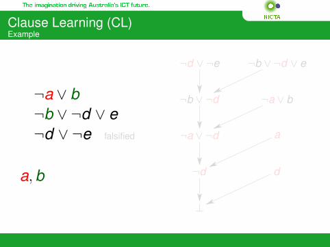
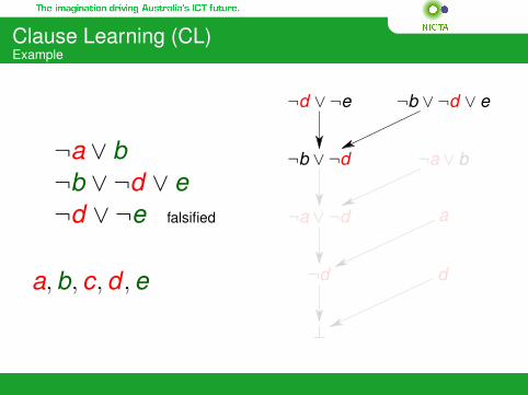
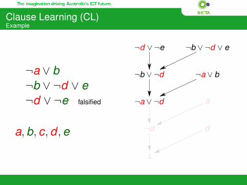
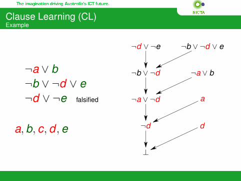
Clause Learning (CL)Example
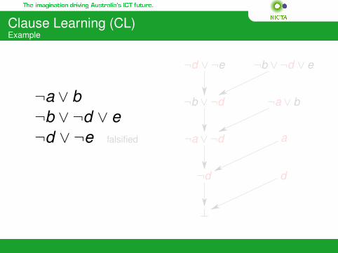
¬a ∨ b¬b ∨ ¬d ∨ e¬d ∨ ¬e falsified
¬d ∨ ¬e ¬b ∨ ¬d ∨ e
¬b ∨ ¬d ¬a ∨ b
¬a ∨ ¬d a
d¬d
⊥
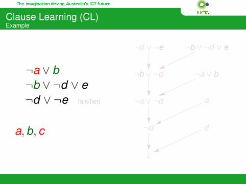
Clause Learning (CL)Example
¬a ∨ b¬b ∨ ¬d ∨ e¬d ∨ ¬e falsified
a, b
¬d ∨ ¬e ¬b ∨ ¬d ∨ e
¬b ∨ ¬d ¬a ∨ b
¬a ∨ ¬d a
d¬d
⊥
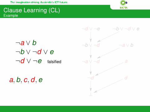
Clause Learning (CL)Example
¬a ∨ b¬b ∨ ¬d ∨ e¬d ∨ ¬e falsified
a, b, c
¬d ∨ ¬e ¬b ∨ ¬d ∨ e
¬b ∨ ¬d ¬a ∨ b
¬a ∨ ¬d a
d¬d
⊥
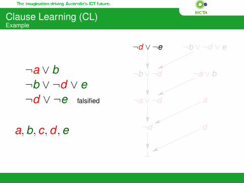
Clause Learning (CL)Example
¬a ∨ b¬b ∨ ¬d ∨ e¬d ∨ ¬e falsified
a, b, c, d , e
¬d ∨ ¬e ¬b ∨ ¬d ∨ e
¬b ∨ ¬d ¬a ∨ b
¬a ∨ ¬d a
d¬d
⊥
Clause Learning (CL)Example
¬a ∨ b¬b ∨ ¬d ∨ e¬d ∨ ¬e falsified
a, b, c, d , e
¬d ∨ ¬e ¬b ∨ ¬d ∨ e
¬b ∨ ¬d ¬a ∨ b
¬a ∨ ¬d a
d¬d
⊥
Clause Learning (CL)Example
¬a ∨ b¬b ∨ ¬d ∨ e¬d ∨ ¬e falsified
a, b, c, d , e
¬d ∨ ¬e ¬b ∨ ¬d ∨ e
¬b ∨ ¬d ¬a ∨ b
¬a ∨ ¬d a
d¬d
⊥
Clause Learning (CL)Example
¬a ∨ b¬b ∨ ¬d ∨ e¬d ∨ ¬e falsified
a, b, c, d , e
¬d ∨ ¬e ¬b ∨ ¬d ∨ e
¬b ∨ ¬d ¬a ∨ b
¬a ∨ ¬d a
d¬d
⊥
Clause Learning (CL)Example
¬a ∨ b¬b ∨ ¬d ∨ e¬d ∨ ¬e falsified
a, b, c, d , e
¬d ∨ ¬e ¬b ∨ ¬d ∨ e
¬b ∨ ¬d ¬a ∨ b
¬a ∨ ¬d a
d¬d
⊥
Clause Learning (CL)Procedure
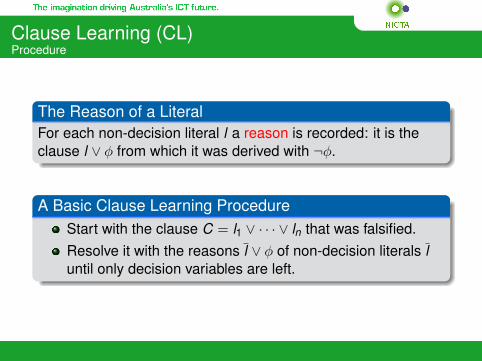
The Reason of a LiteralFor each non-decision literal l a reason is recorded: it is theclause l ∨ φ from which it was derived with ¬φ.
A Basic Clause Learning ProcedureStart with the clause C = l1 ∨ · · · ∨ ln that was falsified.Resolve it with the reasons l ∨ φ of non-decision literals luntil only decision variables are left.
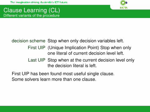
Clause Learning (CL)Different variants of the procedure
decision scheme Stop when only decision variables left.First UIP (Unique Implication Point) Stop when only
one literal of current decision level left.Last UIP Stop when at the current decision level only
the decision literal is left.
First UIP has been found most useful single clause.Some solvers learn more than one clause.

Clause Learning (CL)Forgetting clauses
In contrast to the plain DPLL, a main problem with CL isthe very high number of learned clauses.Most SAT solvers forget clauses exceeding a lengththreshold in a regular interval to prevent the memory fromfilling up.
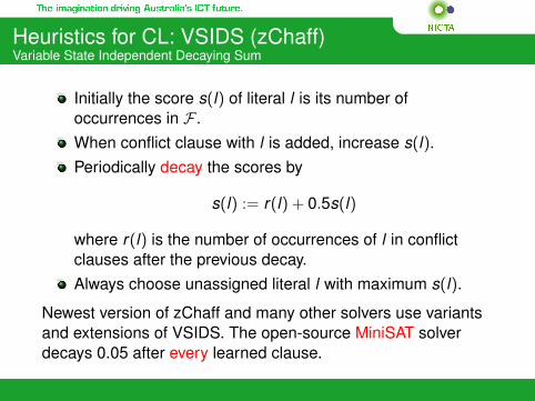
Heuristics for CL: VSIDS (zChaff)Variable State Independent Decaying Sum
Initially the score s(l) of literal l is its number ofoccurrences in F .When conflict clause with l is added, increase s(l).Periodically decay the scores by
s(l) := r(l) + 0.5s(l)
where r(l) is the number of occurrences of l in conflictclauses after the previous decay.Always choose unassigned literal l with maximum s(l).
Newest version of zChaff and many other solvers use variantsand extensions of VSIDS. The open-source MiniSAT solverdecays 0.05 after every learned clause.
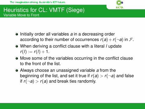
Heuristics for CL: VMTF (Siege)Variable Move to Front
Initially order all variables a in a decreasing orderaccording to their number of occurrences r(a)+ r(¬a) in F .When deriving a conflict clause with a literal l updater(l) := r(l) + 1.Move some of the variables occurring in the conflict clauseto the front of the list.Always choose an unassigned variable a from thebeginning of the list, and set it true if r(a) > r(¬a) and falseif r(¬a) > r(a) and break ties randomly.
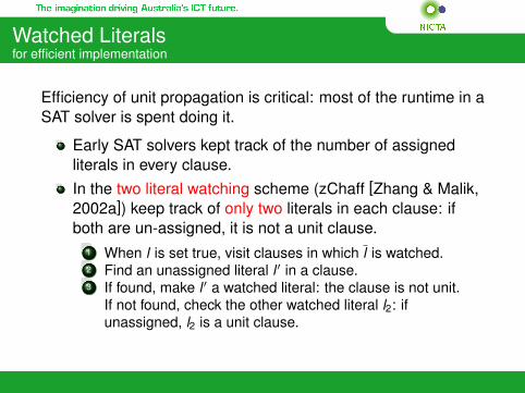
Watched Literalsfor efficient implementation
Efficiency of unit propagation is critical: most of the runtime in aSAT solver is spent doing it.
Early SAT solvers kept track of the number of assignedliterals in every clause.In the two literal watching scheme (zChaff [Zhang & Malik,2002a]) keep track of only two literals in each clause: ifboth are un-assigned, it is not a unit clause.
1 When l is set true, visit clauses in which l is watched.2 Find an unassigned literal l ′ in a clause.3 If found, make l ′ a watched literal: the clause is not unit.
If not found, check the other watched literal l2: ifunassigned, l2 is a unit clause.
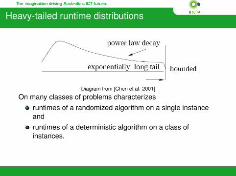
Heavy-tailed runtime distributions
Diagram from [Chen et al. 2001]
On many classes of problems characterizesruntimes of a randomized algorithm on a single instanceandruntimes of a deterministic algorithm on a class ofinstances.
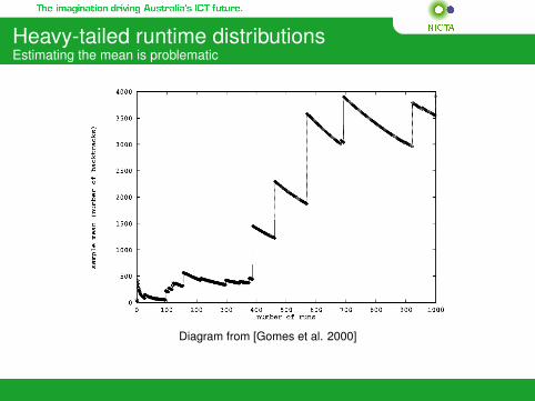
Heavy-tailed runtime distributionsEstimating the mean is problematic
Diagram from [Gomes et al. 2000]
Heavy-tailed runtime distributionsCause
A small number of wrong decisions lead to a part of thesearch tree not containing any solutions.Backtrack-style search needs a long time to traverse thesearch tree.
Many short paths from the root node to a success leafnode.High probability of reaching a huge subtree with nosolutions.
These properties mean thataverage runtime is high,restarting the procedure after t seconds reduces the meansubstantially, if t is close to the mean of the originaldistribution.
Restarts in SAT algorithms
Restarts had been used in stochastic local search algorithms:Necessary for escaping local minima!
Gomes et al. demonstrated the utility of restarts for systematicSAT solvers:
Small amount of randomness in branching variableselection.Restart the algorithm after a given number of seconds.
Restarts with Clause-Learning
Learned clauses are retained when doing the restart.Problem: Optimal restart policy depends on the runtimedistribution, which is generally not known.Problem: Deletion of conflict clauses and too early restartsmay lead to incompleteness. Practical solvers increaserestart interval.Paper: The effect of restarts on the efficiency of clauselearning [Huang, 2007]
Incremental SAT solving
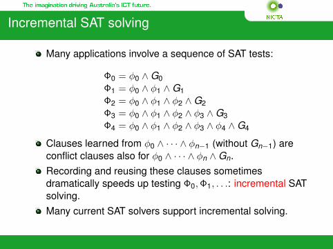
Many applications involve a sequence of SAT tests:
Φ0 = φ0 ∧G0Φ1 = φ0 ∧ φ1 ∧G1Φ2 = φ0 ∧ φ1 ∧ φ2 ∧G2Φ3 = φ0 ∧ φ1 ∧ φ2 ∧ φ3 ∧G3Φ4 = φ0 ∧ φ1 ∧ φ2 ∧ φ3 ∧ φ4 ∧G4
Clauses learned from φ0 ∧ · · · ∧ φn−1 (without Gn−1) areconflict clauses also for φ0 ∧ · · · ∧ φn ∧Gn.Recording and reusing these clauses sometimesdramatically speeds up testing Φ0,Φ1, . . .: incremental SATsolving.Many current SAT solvers support incremental solving.
Preprocessing
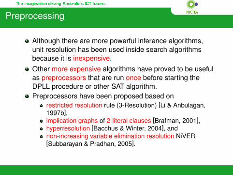
Although there are more powerful inference algorithms,unit resolution has been used inside search algorithmsbecause it is inexpensive.Other more expensive algorithms have proved to be usefulas preprocessors that are run once before starting theDPLL procedure or other SAT algorithm.Preprocessors have been proposed based on
restricted resolution rule (3-Resolution) [Li & Anbulagan,1997b],implication graphs of 2-literal clauses [Brafman, 2001],hyperresolution [Bacchus & Winter, 2004], andnon-increasing variable elimination resolution NiVER[Subbarayan & Pradhan, 2005].

3-Resolution
Adding resolvents for clauses of length ≤ 3.
(x1 ∨ x2 ∨ x3) ∧(x1 ∨ x2 ∨ x4) ≡(x2 ∨ x3 ∨ x4)
2-SIMPLIFY [Brafman, 2001]
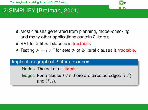
Most clauses generated from planning, model-checkingand many other applications contain 2 literals.SAT for 2-literal clauses is tractable.Testing F |= l ∨ l ′ for sets F of 2-literal clauses is tractable.
Implication graph of 2-literal clausesNodes The set of all literals.Edges For a clause l ∨ l ′ there are directed edges (l , l ′)
and (l ′, l).
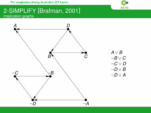
2-SIMPLIFY [Brafman, 2001]Implication graphs
A
B C
D
¬A
¬B¬C
¬D
A ∨ B¬B ∨ C¬C ∨ D¬D ∨ B¬D ∨ A
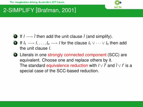
2-SIMPLIFY [Brafman, 2001]
1 If l −→ l then add the unit clause l (and simplify).2 If l1 −→ l , . . . , ln −→ l for the clause l1 ∨ · · · ∨ ln then add
the unit clause l .3 Literals in one strongly connected component (SCC) are
equivalent. Choose one and replace others by it.The standard equivalence reduction with l ∨ l ′ and l ∨ l ′ is aspecial case of the SCC-based reduction.
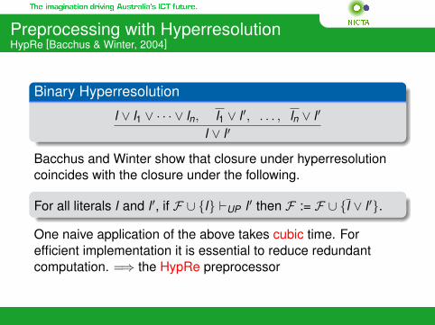
Preprocessing with HyperresolutionHypRe [Bacchus & Winter, 2004]
Binary Hyperresolution
l ∨ l1 ∨ · · · ∨ ln, l1 ∨ l ′, . . . , ln ∨ l ′
l ∨ l ′
Bacchus and Winter show that closure under hyperresolutioncoincides with the closure under the following.
For all literals l and l ′, if F ∪ {l} `UP l ′ then F := F ∪ {l ∨ l ′}.
One naive application of the above takes cubic time. Forefficient implementation it is essential to reduce redundantcomputation. =⇒ the HypRe preprocessor

Preprocessing with ResolutionNon-increasing Variable Elimination Resolution [Subbarayan & Pradhan, 2005]
With unrestricted resolution (the original Davis-Putnamprocedure) clause sets often grow exponentially.Idea: Eliminate a variable if clause set does not grow.
NiVER1 Choose variable a.
F a = {C ∈ F|a is one disjunct of C} andF¬a = {C ∈ F|¬a is one disjunct of C}.
2 OLD = F a ∪ F¬a
NEW = {φ1 ∨ φ2|φ1 ∨ a ∈ F a, φ2 ∨ ¬a ∈ F¬a}.3 If OLD is bigger than NEW , then F := (F\OLD) ∪ NEW .

Algorithms for SAT Solving
Stochastic Methods
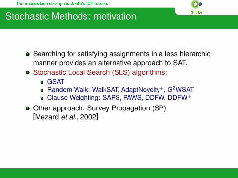
Stochastic Methods: motivation
Searching for satisfying assignments in a less hierarchicmanner provides an alternative approach to SAT.Stochastic Local Search (SLS) algorithms:
GSATRandom Walk: WalkSAT, AdaptNovelty+, G2WSATClause Weighting: SAPS, PAWS, DDFW, DDFW+
Other approach: Survey Propagation (SP)[Mezard et al., 2002]
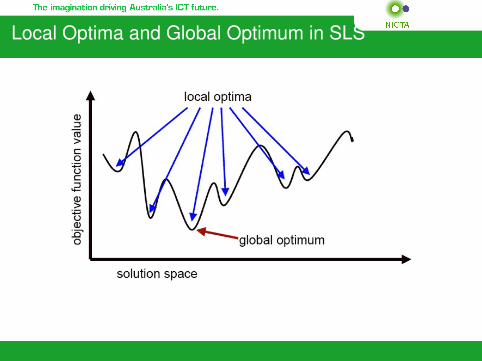
Local Optima and Global Optimum in SLS

Flipping Coins: The “Greedy” Algorithm
This algorithm is due to Koutsopias and PapadimitriouMain idea: flip variables till you can no longer increase thenumber of satisfied clauses.
Procedure greedy(F)1: T = random(F) // random assignment2: repeat3: Flip any variable in T that increases the number of
satisfied clauses;4: until no improvement possible5: end
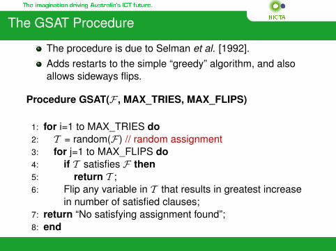
The GSAT Procedure
The procedure is due to Selman et al. [1992].Adds restarts to the simple “greedy” algorithm, and alsoallows sideways flips.
Procedure GSAT(F , MAX_TRIES, MAX_FLIPS)
1: for i=1 to MAX_TRIES do2: T = random(F) // random assignment3: for j=1 to MAX_FLIPS do4: if T satisfies F then5: return T ;6: Flip any variable in T that results in greatest increase
in number of satisfied clauses;7: return “No satisfying assignment found”;8: end
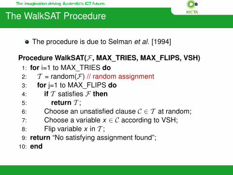
The WalkSAT Procedure
The procedure is due to Selman et al. [1994]
Procedure WalkSAT(F , MAX_TRIES, MAX_FLIPS, VSH)1: for i=1 to MAX_TRIES do2: T = random(F) // random assignment3: for j=1 to MAX_FLIPS do4: if T satisfies F then5: return T ;6: Choose an unsatisfied clause C ∈ T at random;7: Choose a variable x ∈ C according to VSH;8: Flip variable x in T ;9: return “No satisfying assignment found”;
10: end
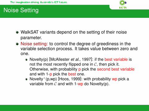
Noise Setting
WalkSAT variants depend on the setting of their noiseparameter.Noise setting: to control the degree of greediness in thevariable selection process. It takes value between zero andone.
Novelty(p) [McAllester et al., 1997]: if the best variable isnot the most recently flipped one in C, then pick it.Otherwise, with probability p pick the second best variableand with 1-p pick the best one.Novelty+(p,wp) [Hoos, 1999]: with probability wp pick avariable from C and with 1-wp do Novelty(p).

AdaptNovelty+
[Hoos, 2002]
AdaptNovelty+ automatically adjusts the noise level based onthe detection of stagnation.
Using Novelty+
in the beginning of a run, noise parameter wp is set to 0.if no improvement in the objective function value duringθ ·m search steps, then increase wp:wp = wp + (1− wp) · φ.if the objective function value is improved, then decreasewp: wp = wp − wp · φ/2.default values: θ = 1/6 and φ = 0.2.
G2WSAT and AdaptG2WSAT
G2WSAT [Li & Huang, 2005]: exploits promisingdecreasing variables and thus diminishes the dependenceon noise settings.AdaptG2WSAT [Li et al., 2007]: integrates the adaptivenoise mechanism of AdaptNovelty+ in G2WSAT.The current best variants of Random Walk approach.
Dynamic Local SearchThe Basic Idea
Use clause weighting mechanismIncrease weights on unsatisfied clauses in local minima insuch a way that further improvement steps becomepossibleAdjust weights periodically when no further improvementsteps are available in the local neighborhood
Dynamic Local SearchBrief History
Breakout Method [Morris, 1993]
Weighted GSAT [Selman et al., 1993]
Learning short-term clause weights for GSAT [Frank, 1997]
Discrete Lagrangian Method (DLM) [Wah & Shang, 1998]
Smoothed Descent and Flood [Schuurmans & Southey, 2000]
Scaling and Probabilistic Smoothing (SAPS) [Hutter et al., 2002]
Pure Additive Weighting Scheme (PAWS) [Thornton et al., 2004]
Divide and Distribute Fixed Weight (DDFW) [Ishtaiwi et al., 2005]
Adaptive DDFW (DDFW+) [Ishtaiwi et al., 2006]
DDFW+: Adaptive DDFW[Ishtaiwi et al., 2006]
Based on DDFW [Ishtaiwi et al., 2005]
No parameter tuningDynamically alters the total amount of weight that DDFWdistributes according to the degree of stagnation in thesearchThe weight of each clause is initialized to 2 and could bealtered during the search between 2 and 3Escapes local minima by transfering weight from satisfiedto unsatisfied clausesExploits the neighborhood relationships between clauseswhen deciding which pairs of clauses will exchange weightR+DDFW+ is among the best SLS solvers for solvingrandom and structured problems
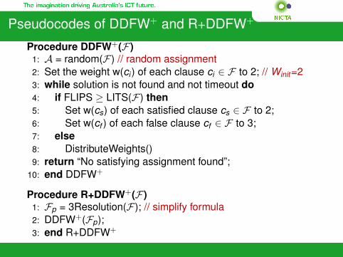
Pseudocodes of DDFW+ and R+DDFW+
Procedure DDFW+(F)1: A = random(F) // random assignment2: Set the weight w(ci ) of each clause ci ∈ F to 2; // Winit=23: while solution is not found and not timeout do4: if FLIPS ≥ LITS(F) then5: Set w(cs) of each satisfied clause cs ∈ F to 2;6: Set w(cf ) of each false clause cf ∈ F to 3;7: else8: DistributeWeights()9: return “No satisfying assignment found”;
10: end DDFW+
Procedure R+DDFW+(F)1: Fp = 3Resolution(F); // simplify formula2: DDFW+(Fp);3: end R+DDFW+
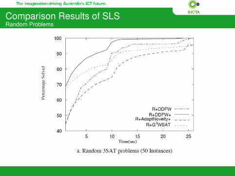
Comparison Results of SLSRandom Problems
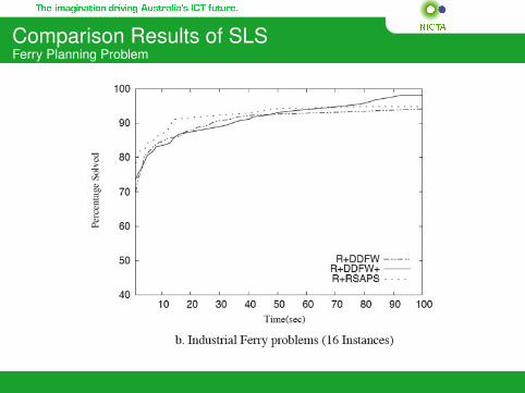
Comparison Results of SLSFerry Planning Problem
Hybrid Approaches
Boosting SLS using Resolution
Paper: “Old Resolution Meets Modern SLS”[Anbulagan et al., 2005]Paper: “Boosting Local Search Performance byIncorporating Resolution-based Preprocessor”[Anbulagan et al., 2006]
Boosting DPLL using Resolution
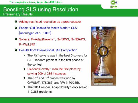
Boosting SLS using ResolutionPreliminary Results
Adding restricted resolution as a preprocessor
Paper: “Old Resolution Meets Modern SLS”
[Anbulagan et al., 2005]
Solvers: R+AdaptNovelty+, R+PAWS, R+RSAPS,
R+WalkSAT
Results from International SAT Competition
The R+* solvers was in the best 5 solvers forSAT Random problem in the first phase ofthe contestR+AdaptNovelty+ won the first place bysolving 209 of 285 instances.The 2nd and 3rd places was won byG2WSAT (178/285) and VW (170/285).The 2004 winner, AdaptNovelty+ only solved119/285 problems.
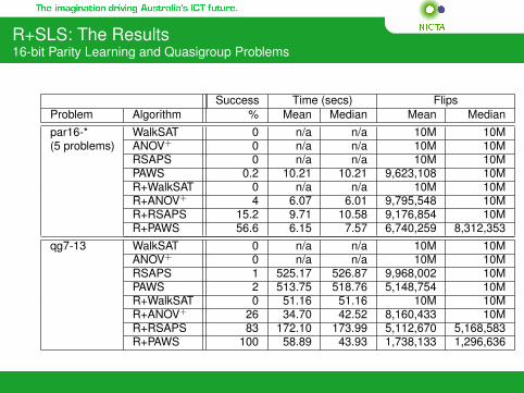
R+SLS: The Results16-bit Parity Learning and Quasigroup Problems
Success Time (secs) FlipsProblem Algorithm % Mean Median Mean Medianpar16-* WalkSAT 0 n/a n/a 10M 10M(5 problems) ANOV+ 0 n/a n/a 10M 10M
RSAPS 0 n/a n/a 10M 10MPAWS 0.2 10.21 10.21 9,623,108 10MR+WalkSAT 0 n/a n/a 10M 10MR+ANOV+ 4 6.07 6.01 9,795,548 10MR+RSAPS 15.2 9.71 10.58 9,176,854 10MR+PAWS 56.6 6.15 7.57 6,740,259 8,312,353
qg7-13 WalkSAT 0 n/a n/a 10M 10MANOV+ 0 n/a n/a 10M 10MRSAPS 1 525.17 526.87 9,968,002 10MPAWS 2 513.75 518.76 5,148,754 10MR+WalkSAT 0 51.16 51.16 10M 10MR+ANOV+ 26 34.70 42.52 8,160,433 10MR+RSAPS 83 172.10 173.99 5,112,670 5,168,583R+PAWS 100 58.89 43.93 1,738,133 1,296,636
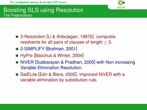
Boosting SLS using ResolutionThe Preprocessor
3-Resolution [Li & Anbulagan, 1997b]: computesresolvents for all pairs of clauses of length ≤ 3.2-SIMPLIFY [Brafman, 2001]
HyPre [Bacchus & Winter, 2004]
NiVER [Subbarayan & Pradhan, 2005] with Non increasingVariable Elimination Resolution.SatELite [Eén & Biere, 2005]: improved NiVER with avariable elimination by substitution rule.
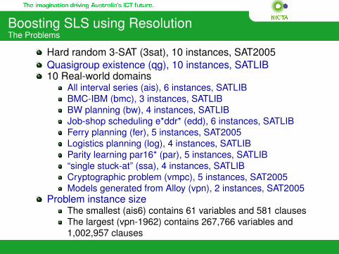
Boosting SLS using ResolutionThe Problems
Hard random 3-SAT (3sat), 10 instances, SAT2005Quasigroup existence (qg), 10 instances, SATLIB10 Real-world domains
All interval series (ais), 6 instances, SATLIBBMC-IBM (bmc), 3 instances, SATLIBBW planning (bw), 4 instances, SATLIBJob-shop scheduling e*ddr* (edd), 6 instances, SATLIBFerry planning (fer), 5 instances, SAT2005Logistics planning (log), 4 instances, SATLIBParity learning par16* (par), 5 instances, SATLIB“single stuck-at” (ssa), 4 instances, SATLIBCryptographic problem (vmpc), 5 instances, SAT2005Models generated from Alloy (vpn), 2 instances, SAT2005
Problem instance sizeThe smallest (ais6) contains 61 variables and 581 clausesThe largest (vpn-1962) contains 267,766 variables and1,002,957 clauses
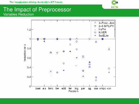
The Impact of PreprocessorVariables Reduction
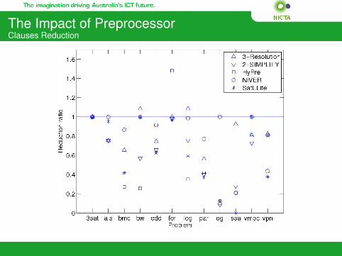
The Impact of PreprocessorClauses Reduction
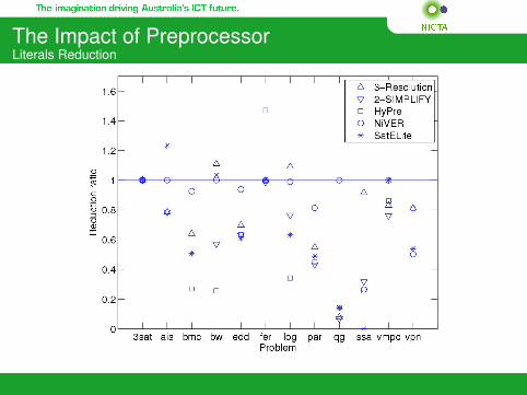
The Impact of PreprocessorLiterals Reduction
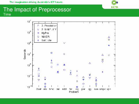
The Impact of PreprocessorTime
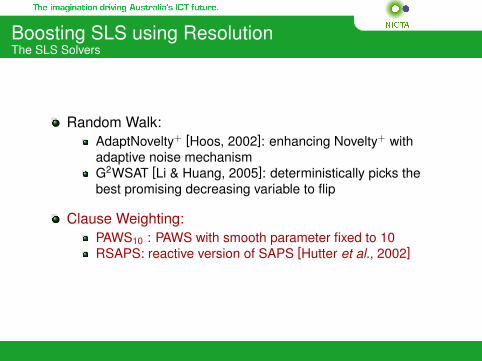
Boosting SLS using ResolutionThe SLS Solvers
Random Walk:AdaptNovelty+ [Hoos, 2002]: enhancing Novelty+ withadaptive noise mechanismG2WSAT [Li & Huang, 2005]: deterministically picks thebest promising decreasing variable to flip
Clause Weighting:PAWS10 : PAWS with smooth parameter fixed to 10RSAPS: reactive version of SAPS [Hutter et al., 2002]
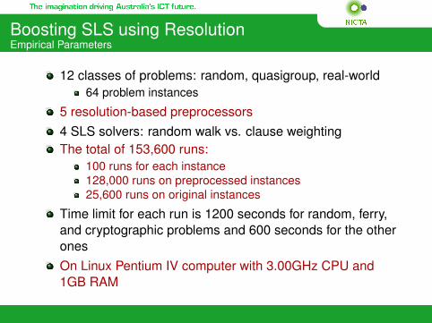
Boosting SLS using ResolutionEmpirical Parameters
12 classes of problems: random, quasigroup, real-world64 problem instances
5 resolution-based preprocessors4 SLS solvers: random walk vs. clause weightingThe total of 153,600 runs:
100 runs for each instance128,000 runs on preprocessed instances25,600 runs on original instances
Time limit for each run is 1200 seconds for random, ferry,and cryptographic problems and 600 seconds for the otheronesOn Linux Pentium IV computer with 3.00GHz CPU and1GB RAM
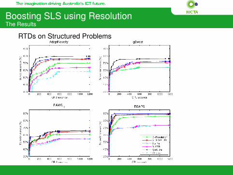
Boosting SLS using ResolutionThe Results
RTDs on Structured Problems

Multiple Preprocessing + SLS
RSAPS performance on ferry planning and par16-4 instancesInstances Preprocessor #Vars/#Cls/#Lits Ptime Succ. CPU Time Flips
rate median mean median mean
ferry7-ks99i origin 1946/22336/45706 n/a 100 192.92 215.27 55, 877, 724 63, 887, 162SatELite 1286/21601/50644 0.27 100 4.39 5.66 897, 165 1, 149, 616HyPre 1881/32855/66732 0.19 100 2.34 3.26 494, 122 684, 276HyPre+Sat 1289/29078/76551 0.72 100 2.17 3.05 359, 981 499, 964Sat+HyPre 1272/61574/130202 0.59 100 0.83 1.17 83, 224 114, 180
ferry8-ks99i origin 2547/32525/66425 n/a 42 1, 200.00 910.38 302, 651, 507 229, 727, 5142-SIMPLIFY 2521/32056/65497 0.08 58 839.26 771.62 316, 037, 896 287, 574, 563SatELite 1696/31589/74007 0.41 100 44.96 58.65 7, 563, 160 9, 812, 123HyPre 2473/48120/97601 0.29 100 9.50 19.61 1, 629, 417 3, 401, 9132-SIM+Sat 1693/31181/73249 0.45 100 14.93 21.63 4, 884, 192 7, 057, 345HyPre+Sat 1700/43296/116045 1.05 100 5.19 10.86 1, 077, 364 2, 264, 998Sat+2-SIM 1683/83930/178217 0.68 100 3.34 4.91 416, 613 599, 421Sat+HyPre 1680/92321/194966 0.90 100 2.23 3.62 252, 778 407, 258
par16-4 origin 1015/3324/8844 n/a 4 600.00 587.27 273, 700, 514 256, 388, 273HyPre 324/1352/3874 0.01 100 10.14 13.42 5, 230, 084 6, 833, 312SatELite 210/1201/4189 0.05 100 5.25 7.33 2, 230, 524 3, 153, 928Sat+HyPre 210/1210/4207 0.05 100 4.73 6.29 1, 987, 638 2, 655, 296HyPre+Sat 198/1232/4352 0.04 100 1.86 2.80 1, 333, 372 1, 995, 865
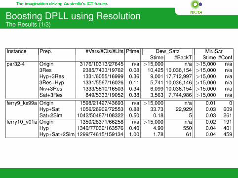
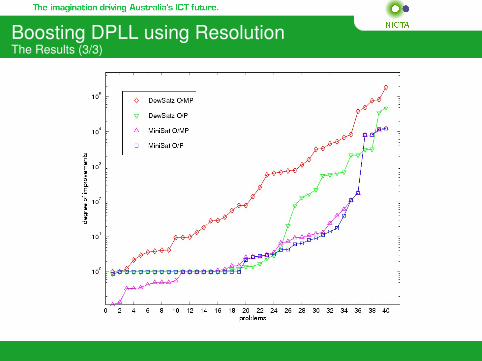
Boosting DPLL using ResolutionThe Results (1/3)
Instance Prep. #Vars/#Cls/#Lits Ptime Dew_Satz MINISAT
Stime #BackT Stime #Confpar32-4 Origin 3176/10313/27645 n/a >15,000 n/a >15,000 n/a
3Res 2385/7433/19762 0.08 10,425 10,036,154 >15,000 n/aHyp+3Res 1331/6055/16999 0.36 9,001 17,712,997 >15,000 n/a3Res+Hyp 1331/5567/16026 0.11 5,741 10,036,146 >15,000 n/aNiv+3Res 1333/5810/16503 0.34 6,099 10,036,154 >15,000 n/aSat+3Res 849/5333/19052 0.38 3,563 7,744,986 >15,000 n/a
ferry9_ks99a Origin 1598/21427/43693 n/a >15,000 n/a 0.01 0Hyp+Sat 1056/26902/72553 0.88 33.73 22,929 0.03 609Sat+2Sim 1042/50487/108322 0.50 0.18 5 0.03 261
ferry10_v01a Origin 1350/28371/66258 n/a >15,000 n/a 0.02 191Hyp 1340/77030/163576 0.40 4.90 550 0.04 401Hyp+Sat+2Sim 1299/74615/159134 1.00 1.78 61 0.04 459

Boosting DPLL using ResolutionThe Results (2/3)
Instance Prep. #Vars/#Cls/#Lits Ptime Dew_Satz MINISATStime #BackT Stime #Conf
bmc-IBM-12 Origin 39598/194778/515536 n/a >15,000 n/a 8.41 11,887Sat 15176/109121/364968 4.50 >15,000 n/a 2.37 6,219Niv+Hyp+3Res 12001/100114/253071 85.81 106 6 0.76 1,937
bmc-IBM-13 Origin 13215/65728/174164 n/a >15,000 n/a 1.84 8,0883Res+Niv+Hyp+3Res 3529/22589/62633 2.90 1,575 4,662,067 0.03 150
bmc-alpha-25449 Origin 663443/3065529/7845396 n/a >15,000 n/a 6.64 502Sat 12408/76025/247622 129 6.94 7 0.06 1Sat+Niv 12356/75709/246367 130 4.48 2 0.06 1
bmc-alpha-4408 Origin 1080015/3054591/7395935 n/a >15,000 n/a 5,409 587,755Sat 23657/112343/364874 47.22 >15,000 n/a 1,266 820,043Sat+2Sim+3Res 16837/98726/305057 52.89 >15,000 n/a 571 510,705
Boosting DPLL using ResolutionThe Results (3/3)
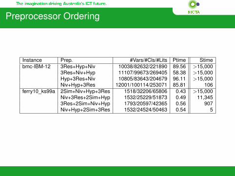
Preprocessor Ordering
Instance Prep. #Vars/#Cls/#Lits Ptime Stimebmc-IBM-12 3Res+Hyp+Niv 10038/82632/221890 89.56 >15,000
3Res+Niv+Hyp 11107/99673/269405 58.38 >15,000Hyp+3Res+Niv 10805/83643/204679 96.11 >15,000Niv+Hyp+3Res 12001/100114/253071 85.81 106
ferry10_ks99a 2Sim+Niv+Hyp+3Res 1518/32206/65806 0.43 >15,000Niv+3Res+2Sim+Hyp 1532/25229/51873 0.49 11,3453Res+2Sim+Niv+Hyp 1793/20597/42365 0.56 907Niv+Hyp+2Sim+3Res 1532/24524/50463 0.54 5

Applications of SAT
equivalence checking for combinational circuitsAI planningLTL model-checkingdiagnosis (static and dynamic)haplotype inference in bioinformatics
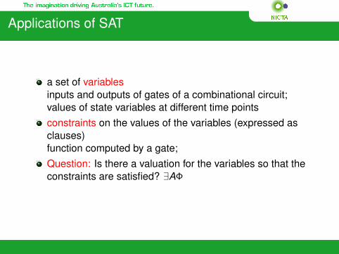
Applications of SAT
a set of variablesinputs and outputs of gates of a combinational circuit;values of state variables at different time pointsconstraints on the values of the variables (expressed asclauses)function computed by a gate;Question: Is there a valuation for the variables so that theconstraints are satisfied? ∃AΦ

Boundaries of SAT
a Generalized Question: ∃A1∀A2∃A3 · · · ∃AnΦ
This is quantified Boolean formulae QBF.Applications:
planning with nondeterminism: there is a plan such thatfor all initial states and contingenciesthere is an execution leading to a goal state.(Also: homing/reset sequences of transition systems)CTL model-checking: ∃ and ∀ are needed for encoding pathquantification.
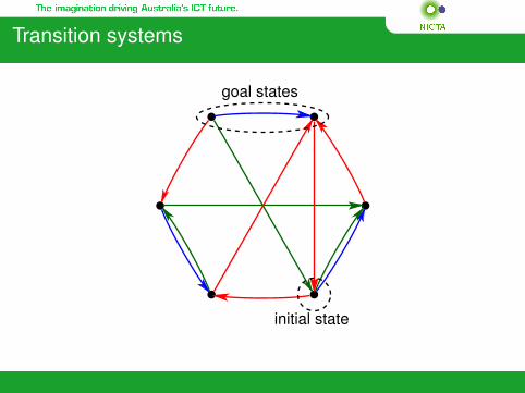
Transition systems
initial state
goal states
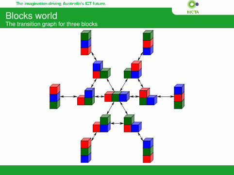
Blocks worldThe transition graph for three blocks

Paths with a given property
A central question about transition systems: is there a pathsatisfying a property P?
application different properties Pplanning (AI): last state satisfies goal G
model-checking (CAV): program specification is violateddiagnosis: compatible with observations; n faults
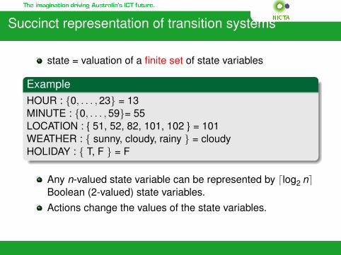
Succinct representation of transition systems
state = valuation of a finite set of state variables
ExampleHOUR : {0, . . . , 23} = 13MINUTE : {0, . . . , 59}= 55LOCATION : { 51, 52, 82, 101, 102 } = 101WEATHER : { sunny, cloudy, rainy } = cloudyHOLIDAY : { T, F } = F
Any n-valued state variable can be represented by dlog2 neBoolean (2-valued) state variables.Actions change the values of the state variables.
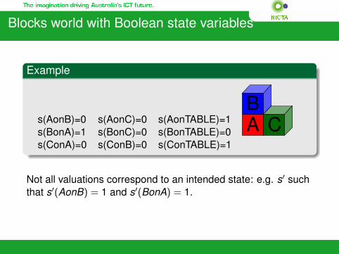
Blocks world with Boolean state variables
Example
s(AonB)=0 s(AonC)=0 s(AonTABLE)=1s(BonA)=1 s(BonC)=0 s(BonTABLE)=0s(ConA)=0 s(ConB)=0 s(ConTABLE)=1
AB
C
Not all valuations correspond to an intended state: e.g. s′ suchthat s′(AonB) = 1 and s′(BonA) = 1.
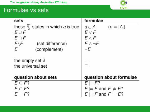
Formulae vs sets
sets formulaethose 2n
2 states in which a is true a ∈ A (n = |A|)E ∪ F E ∨ FE ∩ F E ∧ FE\F (set difference) E ∧ ¬FE (complement) ¬E
the empty set ∅ ⊥the universal set >
question about sets question about formulaeE ⊆ F? E |= F?E ⊂ F? E |= F and F 6|= E?E = F? E |= F and F |= E?
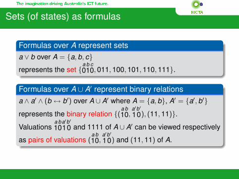
Sets (of states) as formulas
Formulas over A represent setsa ∨ b over A = {a, b, c}
represents the set {a0
b1
c0, 011, 100, 101, 110, 111}.
Formulas over A ∪ A′ represent binary relationsa ∧ a′ ∧ (b ↔ b′) over A ∪ A′ where A = {a, b}, A′ = {a′, b′}
represents the binary relation {(a1
b0,
a′
1b′
0), (11, 11)}.
Valuationsa1
b0
a′
1b′
0 and 1111 of A ∪ A′ can be viewed respectively
as pairs of valuations (a1
b0,
a′
1b′
0) and (11, 11) of A.
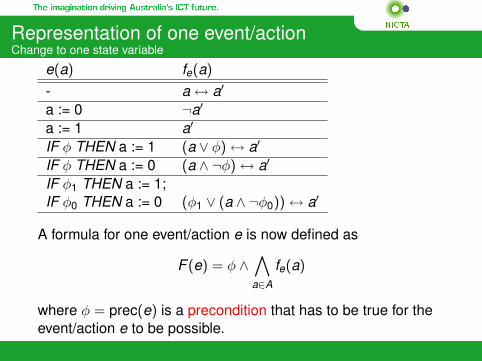
Representation of one event/actionChange to one state variable
e(a) fe(a)
- a ↔ a′
a := 0 ¬a′
a := 1 a′
IF φ THEN a := 1 (a ∨ φ) ↔ a′
IF φ THEN a := 0 (a ∧ ¬φ) ↔ a′
IF φ1 THEN a := 1;IF φ0 THEN a := 0 (φ1 ∨ (a ∧ ¬φ0)) ↔ a′
A formula for one event/action e is now defined as
F (e) = φ ∧∧a∈A
fe(a)
where φ = prec(e) is a precondition that has to be true for theevent/action e to be possible.
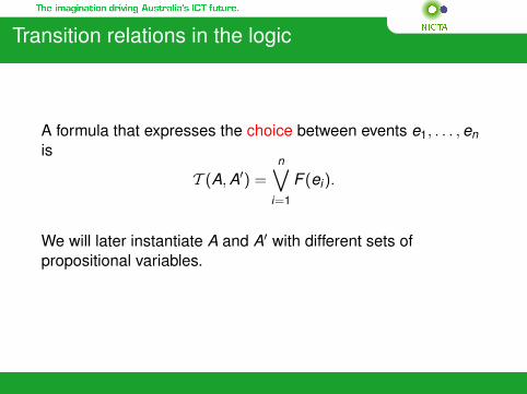
Transition relations in the logic
A formula that expresses the choice between events e1, . . . , enis
T (A, A′) =n∨
i=1
F (ei).
We will later instantiate A and A′ with different sets ofpropositional variables.
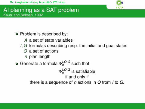
AI planning as a SAT problemKautz and Selman, 1992
Problem is described by:A a set of state variables
I, G formulas describing resp. the initial and goal statesO a set of actionsn plan length
Generate a formula ΦI,O,Gn such that
ΦI,O,Gn is satisfiable
if and only ifthere is a sequence of n actions in O from I to G.

Existence of plans of length n
Propositional variables
Define Ai = {ai |a ∈ A} for all i ∈ {0, . . . , n}.ai expresses the value of a ∈ A at time i .
Plans of length n in the propositional logicPlans of length n correspond to satisfying valuations of
ΦI,O,Gn = I0 ∧ T (A0, A1) ∧ T (A1, A2) ∧ · · · ∧ T (An−1, An) ∧Gn
where for any formula φ by φi we denote φ with propositionalvariables a replaced by ai .

Planning as satisfiabilityExample
ExampleConsider
I = b ∧ cG = (b ∧ ¬c) ∨ (¬b ∧ c)o1 = IF c THEN ¬c; IF ¬c THEN co2 = IF b THEN ¬b; IF ¬b THEN b
Formula for plans of length 3 is
(b0 ∧ c0)∧(((b0 ↔ b1) ∧ (c0 ↔ ¬c1)) ∨ ((b0 ↔ ¬b1) ∧ (c0 ↔ c1)))∧(((b1 ↔ b2) ∧ (c1 ↔ ¬c2)) ∨ ((b1 ↔ ¬b2) ∧ (c1 ↔ c2)))∧(((b2 ↔ b3) ∧ (c2 ↔ ¬c3)) ∨ ((b2 ↔ ¬b3) ∧ (c2 ↔ c3)))∧((b3 ∧ ¬c3) ∨ (¬b3 ∧ c3)).

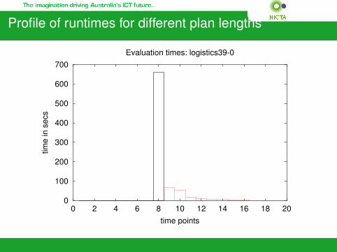
Profile of runtimes for different plan lengths
0
5
10
15
20
25
30
35
40
0 10 20 30 40 50 60 70 80 90 100
time
in s
ecs
time points
Evaluation times: blocks22
Profile of runtimes for different plan lengths
0
100
200
300
400
500
600
700
0 2 4 6 8 10 12 14 16 18 20
time
in s
ecs
time points
Evaluation times: logistics39-0
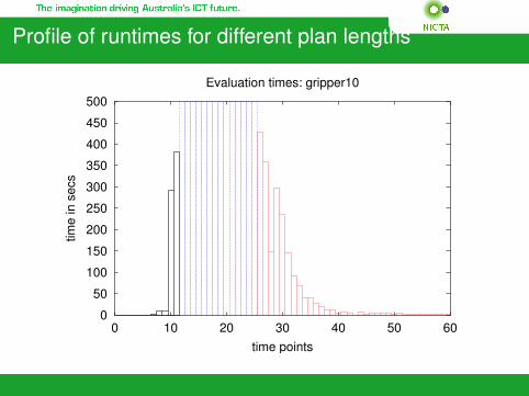
Profile of runtimes for different plan lengths
0
50
100
150
200
250
300
350
400
450
500
0 10 20 30 40 50 60
time
in s
ecs
time points
Evaluation times: gripper10
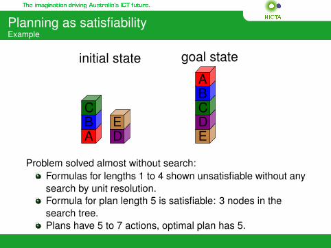
Planning as satisfiabilityExample
ABC
DE
ABCDE
initial state goal state
Problem solved almost without search:Formulas for lengths 1 to 4 shown unsatisfiable without anysearch by unit resolution.Formula for plan length 5 is satisfiable: 3 nodes in thesearch tree.Plans have 5 to 7 actions, optimal plan has 5.

Planning as satisfiabilityExample
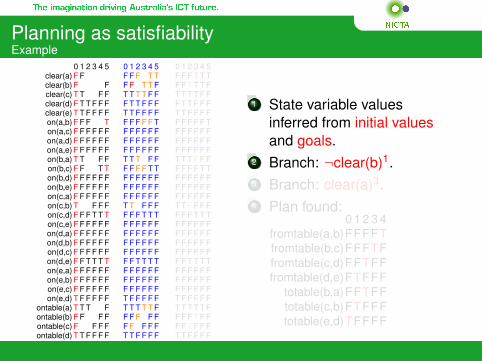
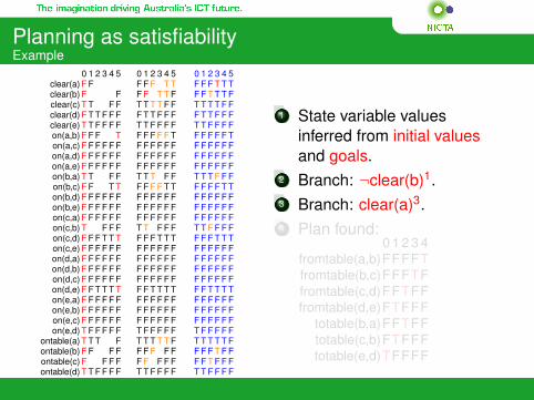
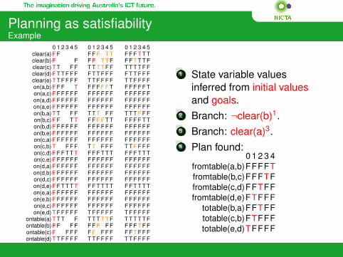
0 1 2 3 4 5clear(a) F Fclear(b) F Fclear(c) T T F Fclear(d) F T T F F Fclear(e) T T F F F Fon(a,b) F F F Ton(a,c) F F F F F Fon(a,d) F F F F F Fon(a,e) F F F F F Fon(b,a) T T F Fon(b,c) F F T Ton(b,d) F F F F F Fon(b,e) F F F F F Fon(c,a) F F F F F Fon(c,b) T F F Fon(c,d) F F F T T Ton(c,e) F F F F F Fon(d,a) F F F F F Fon(d,b) F F F F F Fon(d,c) F F F F F Fon(d,e) F F T T T Ton(e,a) F F F F F Fon(e,b) F F F F F Fon(e,c) F F F F F Fon(e,d) T F F F F F
ontable(a) T T T Fontable(b) F F F Fontable(c) F F F Fontable(d) T T F F F Fontable(e) F T T T T T
0 1 2 3 4 5F F F T TF F T T FT T T T F FF T T F F FT T F F F FF F F F F TF F F F F FF F F F F FF F F F F FT T T F FF F F F T TF F F F F FF F F F F FF F F F F FT T F F FF F F T T TF F F F F FF F F F F FF F F F F FF F F F F FF F T T T TF F F F F FF F F F F FF F F F F FT F F F F FT T T T T FF F F F FF F F F FT T F F F FF T T T T T
0 1 2 3 4 5F F F T T TF F T T T FT T T T F FF T T F F FT T F F F FF F F F F TF F F F F FF F F F F FF F F F F FT T T F F FF F F F T TF F F F F FF F F F F FF F F F F FT T F F F FF F F T T TF F F F F FF F F F F FF F F F F FF F F F F FF F T T T TF F F F F FF F F F F FF F F F F FT F F F F FT T T T T FF F F T F FF F T F F FT T F F F FF T T T T T
1 State variable valuesinferred from initial valuesand goals.
2 Branch: ¬clear(b)1.3 Branch: clear(a)3.4 Plan found:
0 1 2 3 4fromtable(a,b)FFFFTfromtable(b,c)FFFTFfromtable(c,d)FFTFFfromtable(d,e)FTFFF
totable(b,a)FFTFFtotable(c,b)FTFFFtotable(e,d)TFFFF
Planning as satisfiabilityExample
0 1 2 3 4 5clear(a) F Fclear(b) F Fclear(c) T T F Fclear(d) F T T F F Fclear(e) T T F F F Fon(a,b) F F F Ton(a,c) F F F F F Fon(a,d) F F F F F Fon(a,e) F F F F F Fon(b,a) T T F Fon(b,c) F F T Ton(b,d) F F F F F Fon(b,e) F F F F F Fon(c,a) F F F F F Fon(c,b) T F F Fon(c,d) F F F T T Ton(c,e) F F F F F Fon(d,a) F F F F F Fon(d,b) F F F F F Fon(d,c) F F F F F Fon(d,e) F F T T T Ton(e,a) F F F F F Fon(e,b) F F F F F Fon(e,c) F F F F F Fon(e,d) T F F F F F
ontable(a) T T T Fontable(b) F F F Fontable(c) F F F Fontable(d) T T F F F Fontable(e) F T T T T T
0 1 2 3 4 5F F F T TF F T T FT T T T F FF T T F F FT T F F F FF F F F F TF F F F F FF F F F F FF F F F F FT T T F FF F F F T TF F F F F FF F F F F FF F F F F FT T F F FF F F T T TF F F F F FF F F F F FF F F F F FF F F F F FF F T T T TF F F F F FF F F F F FF F F F F FT F F F F FT T T T T FF F F F FF F F F FT T F F F FF T T T T T
0 1 2 3 4 5F F F T T TF F T T T FT T T T F FF T T F F FT T F F F FF F F F F TF F F F F FF F F F F FF F F F F FT T T F F FF F F F T TF F F F F FF F F F F FF F F F F FT T F F F FF F F T T TF F F F F FF F F F F FF F F F F FF F F F F FF F T T T TF F F F F FF F F F F FF F F F F FT F F F F FT T T T T FF F F T F FF F T F F FT T F F F FF T T T T T
1 State variable valuesinferred from initial valuesand goals.
2 Branch: ¬clear(b)1.3 Branch: clear(a)3.4 Plan found:
0 1 2 3 4fromtable(a,b)FFFFTfromtable(b,c)FFFTFfromtable(c,d)FFTFFfromtable(d,e)FTFFF
totable(b,a)FFTFFtotable(c,b)FTFFFtotable(e,d)TFFFF
LTL Model-Checking
Bounded model-checking (1999-, M-USD business) inComputer Aided Verification is a direct offspring ofplanning as satisfiability.A basic model-checking problem for safety properties isidentical to the planning problem: test if there is asequence of transitions that leads to a bad state(corresponding to the goal in planning.)General problem: test whether all executions satisfy agiven property expressed as a temporal logic formula.
Temporal logics
Linear Temporal Logic LTL: properties of transitionsequencesComputation Tree Logics CTL and CTL∗: properties ofcomputation trees, with path quantification for all paths andfor some paths.
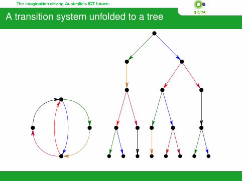
A transition system unfolded to a tree
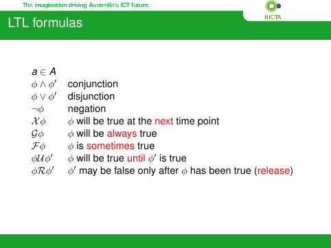
LTL formulas
a ∈ Aφ ∧ φ′ conjunctionφ ∨ φ′ disjunction¬φ negationXφ φ will be true at the next time pointGφ φ will be always trueFφ φ is sometimes trueφUφ′ φ will be true until φ′ is trueφRφ′ φ′ may be false only after φ has been true (release)
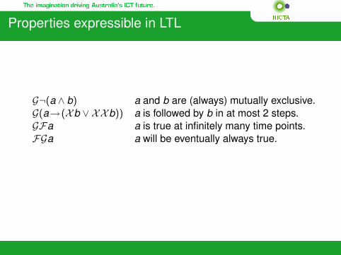
Properties expressible in LTL
G¬(a ∧ b) a and b are (always) mutually exclusive.G(a→(Xb ∨ XXb)) a is followed by b in at most 2 steps.GFa a is true at infinitely many time points.FGa a will be eventually always true.

LTL formulassemantics
v |=i a iff v(a, i) = 1v |=i φ ∧ φ′ iff v |=i φ and v |=i φ′
v |=i φ ∨ φ′ iff v |=i φ or v |=i φ′
v |=i ¬φ iff v 6|=i φv |=i Xφ iff v |=i+1 φv |=i Gφ iff v |=j for all j ≥ iv |=i Fφ iff v |=j for some j ≥ iv |=i φUφ′ iff ∃j ≥ i s.t. v |=j φ′ and v |=k φ for all k ∈ {i , . . . , j − 1}v |=i φRφ′ iff ∀j ≥ i , v |=j φ′ or v |=k φ for some k ∈ {i , . . . , j − 1}

Translating LTL formulas into NNF
In NNF negations occur only in front of atomic formulas. Thiscan be achieved by applying the following equivalences fromleft to right.
¬(φ ∧ φ′) ≡ ¬φ ∨ ¬φ′
¬(φ ∨ φ′) ≡ ¬φ ∧ ¬φ′
¬¬φ ≡ φ¬(Xφ) ≡ X¬φ¬Gφ ≡ F¬φ¬Fφ ≡ G¬φ
¬(φUφ′) ≡ ¬φR¬φ′
¬(φRφ′) ≡ ¬φU¬φ′
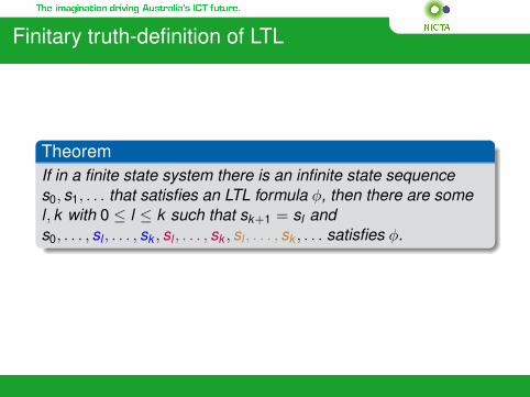
Finitary truth-definition of LTL
TheoremIf in a finite state system there is an infinite state sequences0, s1, . . . that satisfies an LTL formula φ, then there are somel , k with 0 ≤ l ≤ k such that sk+1 = sl ands0, . . . , sl , . . . , sk , sl , . . . , sk , sl , . . . , sk , . . . satisfies φ.
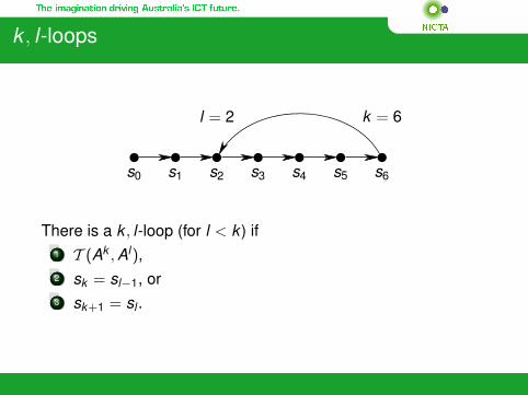
k , l-loops
s0 s1 s2 s3 s4 s5 s6
l = 2 k = 6
There is a k , l-loop (for l < k ) if1 T (Ak , Al),2 sk = sl−1, or3 sk+1 = sl .
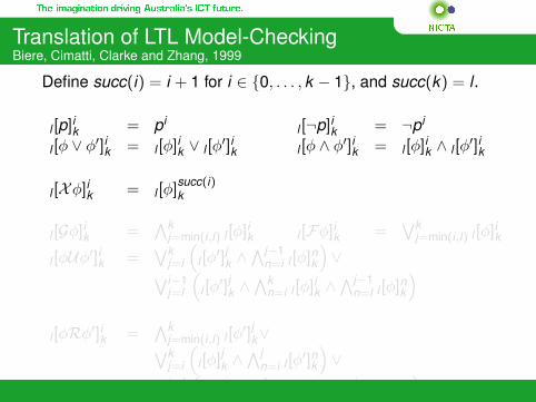
Translation of LTL Model-CheckingBiere, Cimatti, Clarke and Zhang, 1999
Define succ(i) = i + 1 for i ∈ {0, . . . , k − 1}, and succ(k) = l .
l [p]ik = pil [¬p]ik = ¬pi
l [φ ∨ φ′]ik = l [φ]ik ∨ l [φ′]ik l [φ ∧ φ′]ik = l [φ]ik ∧ l [φ
′]ik
l [Xφ]ik = l [φ]succ(i)k
l [Gφ]ik =∧k
j=min(i,l) l [φ]ik l [Fφ]ik =∨k
j=min(i,l) l [φ]ik
l [φUφ′]ik =∨k
j=i
(l [φ
′]jk ∧∧j−1
n=i l [φ]nk
)∨∨i−1
j=l
(l [φ
′]jk ∧∧k
n=i l [φ]ik ∧∧j−1
n=l l [φ]nk
)l [φRφ′]ik =
∧kj=min(i,l) l [φ
′]jk∨∨kj=i
(l [φ]jk ∧
∧jn=i l [φ
′]nk
)∨∨i−1
j=l
(l [φ]jk ∧
∧kn=i l [φ
′]nk ∧∧j
n=l l [φ′]nk
)
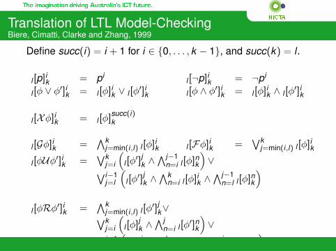
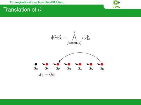
Translation of G
l [Gφ]ik =k∧
j=min(i,l)l [φ]ik
s0 s1 s2 s3 s4 s5 s6
s1 |= Gφ
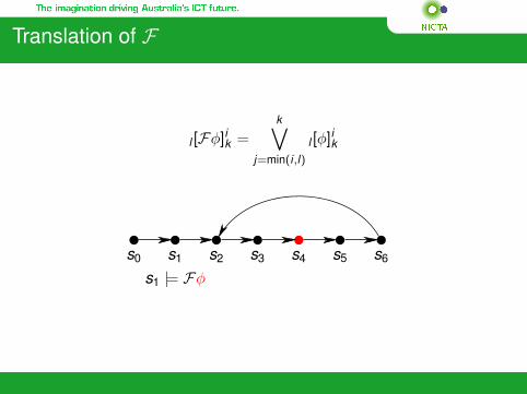
Translation of F
l [Fφ]ik =k∨
j=min(i,l)l [φ]ik
s0 s1 s2 s3 s4 s5 s6
s1 |= Fφ
Translation of U
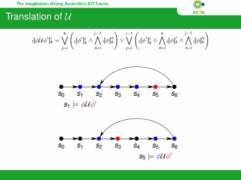
l [φUφ′]ik =k_
j=i
l [φ
′]jk ∧j−1
n=i
l [φ]nk
!∨
i−1_j=l
l [φ
′]jk ∧k
n=i
l [φ]ik ∧j−1
n=l
l [φ]nk
!
s0 s1 s2 s3 s4 s5 s6
s1 |= φUφ′
s0 s1 s2 s3 s4 s5 s6
s5 |= φUφ′
Translation of R
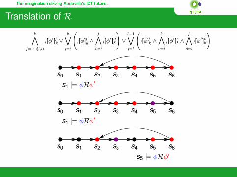
k
j=min(i,l)
l [φ′]jk ∨
k_j=i
l [φ]jk ∧
j
n=i
l [φ′]nk
!∨
i−1_j=l
l [φ]jk ∧
k
n=i
l [φ′]nk ∧
j
n=l
l [φ′]nk
!
s0 s1 s2 s3 s4 s5 s6
s1 |= φRφ′
s0 s1 s2 s3 s4 s5 s6
s1 |= φRφ′
s0 s1 s2 s3 s4 s5 s6
s5 |= φRφ′
LTL model-checking
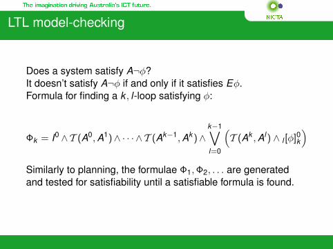
Does a system satisfy A¬φ?It doesn’t satisfy A¬φ if and only if it satisfies Eφ.Formula for finding a k , l-loop satisfying φ:
Φk = I0 ∧T (A0, A1)∧ · · · ∧ T (Ak−1, Ak )∧k−1∨l=0
(T (Ak , Al) ∧ l [φ]0k
)Similarly to planning, the formulae Φ1,Φ2, . . . are generatedand tested for satisfiability until a satisfiable formula is found.
LTL model-checking with finite executions
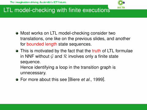
Most works on LTL model-checking consider twotranslations, one like on the previous slides, and anotherfor bounded length state sequences.This is motivated by the fact that the truth of LTL formulaein NNF without G and R involves only a finite statesequence.Hence identifying a loop in the transition graph isunnecessary.For more about this see [Biere et al., 1999].

Other translations
The translation by Biere et al. 1999 has a cubic size.There are much more efficient translations, with linear size[Latvala et al., 2004].
1 Each subformula of φ is represented only once for eachtime point: multiple references to it through an auxiliaryvariable.
2 Existence of a loop is tested by∧k−1
l=0∧
a∈A(al ↔ ak ), andthe translations of the events refer to the loop with auxiliaryvariables which indicate the starting time l .

Diagnosis
diagnosis of static systems: observations are the inputsand outputsdiagnosis of dynamic systems: observations areevents/facts with time tagsvariants of diagnosis:
1 model-based diagnosis, based on a system model2 more heuristic approaches with diagnostic rules, example:
medical diagnosis

Approaches to model-based diagnosis
1 consistency-based diagnosis: A diagnosis corresponds toa valuation that satisfies the formula representing thesystem and the observations.v |= SD ∪OBS
2 abductive diagnosis: A diagnosis is a set S of assumptionsthat together with the formula entail the observations.S ∪ SD |= OBS
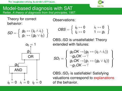
Model-based diagnosis with SATReiter, A theory of diagnosis from first principles, 1987.
Theory for correctbehavior:
SD =
{g0 ↔ (i0 ∧ i1)g1 ↔ (g0 ∨ i2)
}
AND
OR
i0 = 0 i1 = 0 i2 = 0
g0
g1
o0 = 1
Observations:
OBS =
{i0 ↔ 0 i1 ↔ 0i2 ↔ 0 1 ↔ g1
}OBS∪SD is unsatisfiable! Theoryextended with failures:
SDf =
g0OK →(g0 ↔ (i0 ∧ i1))¬g0OK →>g1OK →(g1 ↔ (g0 ∨ i2))¬g1OK →>
OBS∪SDf is satisfiable! Satisfyingvaluations correspond to explanationsof the behavior.

Minimal diagnoses
Assume as few failures as possible (preferably 0).Finding small diagnoses (small number of failures) may bemuch easier than finding bigger ones.This motivates the use of cardinality constraints: find onlydiagnoses with m failures for some (small) m.A cardinality constraint for restricting the number of trueatomic propositions among x1, . . . , xn to ≤ m is denoted bycard(x1, . . . , xn; m).
Minimal diagnosesCardinality constraints
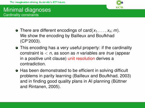
There are different encodings of card(x1, . . . , xn; m).We show the encoding by Bailleux and Boufkhad(CP’2003).This encoding has a very useful property: if the cardinalityconstraint is < n, as soon as n variables are true (appearin a positive unit clause) unit resolution derives acontradiction.Has been demonstrated to be efficient in solving difficultproblems in parity learning (Bailleux and Boufkhad, 2003)and in finding good quality plans in AI planning (Büttnerand Rintanen, 2005).
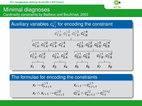
Minimal diagnosesCardinality constraints by Bailleux and Boufkhad, 2003
Auxiliary variables c≥ik :j for encoding the constraint
x1 x2 x3 x4 x5 x6 x7 x8
c≥11:2, c≥2
1:2 c≥13:4, c≥2
3:4 c≥15:6, c≥2
5:6 c≥17:8, c≥2
7:8
c≥11:4, c≥2
1:4, c≥31:4, c≥4
1:4 c≥15:8, c≥2
5:8, c≥35:8, c≥4
5:8
c≥11:8, c≥2
1:8, c≥31:8, c≥4
1:8
The formulae for encoding the constraints
xr →c≥1r :r+1 xr+1→c≥1
r :r+1
xr ∧ xr+1→c≥2r :r+1 c≥i
r :s ∧ c≥js+1:t →c≥i+j
r :t

Minimal diagnosesCardinality constraints by Bailleux and Boufkhad, 2003
φ ∧ card(x1, . . . , x8; 3) ∈ SAT if and only if there is a valuation ofφ with at most 3 of the variables x1, . . . , x8 true.card(x1, . . . , x8; 3) is defined as the conjunction of ¬c≥4
1:8 and
c≥41:4 →c≥4
1:8 c≥45:8 →c≥4
1:8c≥1
1:4 ∧ c≥35:8 →c≥4
1:8 c≥31:4 ∧ c≥1
5:8 →c≥41:8 c≥2
1:4 ∧ c≥25:8 →c≥4
1:8
c≥11:2 →c≥1
1:4 c≥13:4 →c≥1
1:4 c≥15:6 →c≥1
5:8 c≥17:8 →c≥1
5:8c≥2
1:2 →c≥21:4 c≥2
3:4 →c≥21:4 c≥2
5:6 →c≥25:8 c≥2
7:8 →c≥25:8
c≥11:2 ∧ c≥1
3:4 →c≥21:4 c≥1
1:2 ∧ c≥23:4 →c≥3
1:4 c≥15:6 ∧ c≥1
7:8 →c≥25:8 c≥1
5:6 ∧ c≥27:8 →c≥3
5:8
c≥21:2 ∧ c≥1
3:4 →c≥31:4 c≥2
1:2 ∧ c≥23:4 →c≥4
1:4 c≥25:6 ∧ c≥1
7:8 →c≥35:8 c≥2
5:6 ∧ c≥27:8 →c≥4
5:8
x1→c≥11:2 x3→c≥1
3:4 x5→c≥15:6 x7→c≥1
7:8x2→c≥1
1:2 x4→c≥13:4 x6→c≥1
5:6 x8→c≥17:8
x1 ∧ x2→c≥21:2 x3 ∧ x4→c≥2
3:4 x5 ∧ x6→c≥25:6 x7 ∧ x8→c≥2
7:8
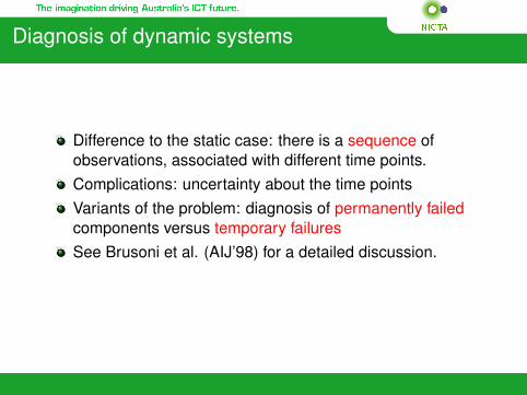
Diagnosis of dynamic systems
Difference to the static case: there is a sequence ofobservations, associated with different time points.Complications: uncertainty about the time pointsVariants of the problem: diagnosis of permanently failedcomponents versus temporary failuresSee Brusoni et al. (AIJ’98) for a detailed discussion.
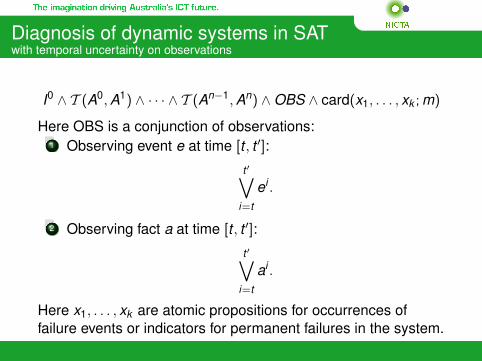
Diagnosis of dynamic systems in SATwith temporal uncertainty on observations
I0 ∧ T (A0, A1) ∧ · · · ∧ T (An−1, An) ∧OBS ∧ card(x1, . . . , xk ; m)
Here OBS is a conjunction of observations:1 Observing event e at time [t , t ′]:
t ′∨i=t
ei .
2 Observing fact a at time [t , t ′]:
t ′∨i=t
ai .
Here x1, . . . , xk are atomic propositions for occurrences offailure events or indicators for permanent failures in the system.

Bibliography I
Anbulagan.Extending Unit Propagation Look-Ahead of DPLL Procedure.In Proc. of the 8th PRICAI, pages 173–182. 2004.
Anbulagan, D. N. Pham, J. Slaney and A. Sattar.Old Resolution Meets Modern SLS.In Proc. of the 20th AAAI, pages 354–359. 2005.
Anbulagan and J. Slaney.Lookahead Saturation with Restriction for SAT.In Proc. of the 11th CP, Sitges, Spain, 2005.
Anbulagan, D. N. Pham, J. Slaney and A. Sattar.Boosting SLS Performance by Incorporating Resolution-based Preprocessor.In Proc. of Third International Workshop on Local Search Techniques inConstraint Satisfaction (LSCS), in conjunction with CP-06, pages 43–57. 2006.
Anbulagan and J. Slaney.Multiple Preprocessing for Systematic SAT Solvers.In Proc. of the 6th International Workshop on the Implementation of Logics(IWIL-6), Phnom Penh, Cambodia, 2006.

Bibliography II
F. Bacchus and J. Winter.Effective Preprocessing with Hyper-Resolution and Equality Reduction.In Revised selected papers from the 6th SAT, pages 341–355. 2004.
O. Bailleux and Y. Boufkhad.Efficient CNF encoding of Boolean cardinality constraints.In Proc. of 9th CP, pages 108–122. 2003.
R. J. Bayardo, Jr. and R. C. Schrag.Using CSP look-back techniques to solve real-world SAT instances.In Proc. of the 14th AAAI, pages 203–208, 1997.
P. Beame, H. Kautz and A. Sabharwal.Towards understanding and harnessing the potential of clause learning.Journal of Artificial Intelligence Research, 22:319–351, 2004.
A. Biere, A. Cimatti, E. M. Clarke and Y. Zhu.Symbolic model checking without BDDs.In Proc. of 5th TACAS, volume 1579 of LNCS, pages 193–207. 1999.
A. Biere.Resolve and expand.In Proc. of 7th SAT, Vancouver, BC, Canada, pages 59–70, 2004.

Bibliography III
R. I. Brafman.A Simplifier for Propositional Formulas with Many Binary Clauses.In Proc. of the 17th IJCAI, pages 515–522. 2001.
H. Chen, C. Gomes and B. Selman.Formal Models of Heavy-Tailed Behavior in Combinatorial Search.In Proc. of the 7th CP, pages 408–421, 2001.
S. A. Cook.The Complexity of Theorem Proving Procedures.In Proc. of the 3rd ACM Symposium on Theory of Computing, 1971.
M. Davis and H. Putnam.A Computing Procedure for Quantification Theory.Journal of the ACM 7:201–215. 1960.
M. Davis, G. Logemann and D. Loveland.A machine program for theorem proving.Communications of ACM 5:394–397. 1962.
O. Dubois, P. Andre, Y. Boufkhad and J. Carlier.SAT versus UNSAT.In Proc. of the 2nd DIMACS Challenge: Cliques, Coloring and Satisfiability. 1993.

Bibliography IVO. Dubois and G. Dequen.A Backbone-search Heuristic for Efficient Solving of hard 3-SAT Formulae.In Proc. of the 17th IJCAI, Seattle, Washington, USA, 2001.
N. Eén and N. Sörensson.Temporal induction by incremental SAT solving.Electronic Notes in Theoretical Computer Science, 89(4):543–560, 2003.
N. Eén and A. Biere.Effective Preprocessing in SAT through Variable and Clause Elimination.In Proc. of the 8th SAT, pages 61–75, 2005.
E. A. Emerson. Temporal and modal logic. In J. Van Leeuwen, editor, Handbookof Theoretical Computer Science, volume B, pages 995–1072. Elsevier SciencePublishers, 1990.
J. Frank.Learning Short-term Clause Weights for GSAT.In Proc. of the 15th IJCAI, pages 384–389, 1997.
E. Giunchiglia, M. Narizzano, and A. Tacchella.Clause/term resolution and learning in the evaluation of quantified Booleanformulas.Journal of Artificial Intelligence Research, 26:371–416, 2006.

Bibliography V
C. P. Gomes, B. Selman, and H. Kautz.Boosting combinatorial search through randomization.In Proc. of the 14th AAAI, pages 431–437. 1998.
C. P. Gomes, B. Selman, N. Crato, and H. Kautz.Heavy-tailed phenomena in satisfiability and constraint satisfaction problems.Journal of Automated Reasoning, 24(1–2):67–100, 2000.
M. Heule and H. van Maaren.March_dl: Adding Adaptive Heuristics and a New Branching Strategy.Journal on Satisfiability, Boolean Modeling and Computation, 2:47–59, 2006.
J. N. Hooker and V. Vinay.Branching Rules for Satisfiability.Journal of Automated Reasoning, 15:359–383, 1995.
H. H. Hoos.On the Run-time Behaviour of Stochastic Local Search Algorithms for SAT.In Proc. of the 16th AAAI, pages 661–666. 1999.
H. H. Hoos.An Adaptive Noise Mechanism for WalkSAT.In Proc. of the 17th AAAI, pages 655–660. 2002.

Bibliography VIJ. Huang.The Effect of Restarts on the Efficiency of Clause Learning.In Proc. of the 20th IJCAI, Hyderabad, India, 2007.
F. Hutter, D. A. D. Tompkins and H. H. Hoos.Scaling and Probabilistic Smoothing: Efficient Dynamic Local Search for SAT.In Proc. of the 8th CP, pages 233–248, Ithaca, New York, USA, 2002.
A. Ishtaiwi, J. Thornton, A. Sattar and D. N. Pham.Neigbourhood Clause Weight Redistribution in Local Search for SAT.In Proc. of the 11th CP, Sitges, Spain, 2005.
A. Ishtaiwi, J. Thornton, Anbulagan, A. Sattar and D. N. Pham.Adaptive Clause Weight Redistribution.In Proc. of the 12th CP, Nantes, France, 2006.
R. Jeroslow and J. Wang.Solving Propositional Satisfiability Problems.Annals of Mathematics and AI, 1:167–187, 1990.
T. Junttila and I. Niemelä.Towards an Efficient Tableau Method for Boolean Circuit Satisfiability Checking.Computational Logic - CL 2000; First International Conference, LNCS 1861,553–567, Springer-Verlag, 2000.

Bibliography VII
B. Jurkowiak, C. M. Li, and G. Utard.A Parallelization Scheme Based on Work Stealing for a Class of SAT Solvers.J. Automated Reasoning, 34:73–101, 2005.
H. Kautz and B. Selman.Pushing the envelope: planning, propositional logic, and stochastic search.In Proc. of the 13th AAAI, pages 1194–1201. 1996.
H. Kautz and B. Selman.Ten Challenges Redux: Recent Progress in Propositional Reasoning and Search.
In Proc. of the 9th CP, Kinsale, County Cork, Ireland, 2003.
P. Kilby, J. Slaney, S. Thiébaux and T. Walsh.Backbones and Backdoors in Satisfiability.In Proc. of the 20th AAAI, pages 1368–1373. 2005.
T. Latvala, A. Biere, K. Heljanko and T. Junttila.Simple Bounded LTL Model-Checking.In Proc. 5th FMCAD’04, pages 186–200, 2004.

Bibliography VIII
C. M. Li and Anbulagan.Heuristics based on unit propagation for satisfiability problems.In Proc. of the 15th IJCAI, pages 366–371, Nagoya, Japan. 1997.
C. M. Li and Anbulagan.Look-Ahead Versus Look-Back for Satisfiability Problems.In Proc. of the 3rd CP, pages 341–355, Schloss Hagenberg, Austria, 1997.
C. M. Li.Integrating Equivalency Reasoning into Davis-Putnam Procedure.In Proc. of 17th AAAI, pages 291–296, 2000.
C. M. Li and W. Q. Huang.Diversification and Determinism in Local Search for Satisfiability.In Proc. of the 8th SAT, pages 158–172. 2005.
C. M. Li, F. Manyá and J. Planes.Detecting Disjoint Inconsistent Subformulas for Computing Lower Bounds forMax-SAT.In Proc. of the 21st AAAI, 2006.
Bibliography IX
C. M. Li, W. Wei and H. Zhang.Combining Adaptive Noise and Look-Ahead in Local Search for SAT.In Proc. of the 10th SAT, pages 121–133. 2007.
J. P. Marques-Silva and K. A. Sakallah.GRASP: A new search algorithm for satisfiability.In Proc. of ICCAD, pages 220–227, 1996.
D. McAllester, B. Selman and H. Kautz.Evidence for Invariants in Local Search.In Proc. of the 14th AAAI, pages 321–326. 1997.
M. Mezard, G. Parisi and R. Zecchina.Analytic and Algorithmic Solution of Random Satisfiability Problems.In Science, 297(5582), pages 812–815. 2002.
D. Mitchell, B. Selman and H. Levesque.Hard and Easy Distributions of SAT Problems.In Proc. of the 10th AAAI, pages 459–465, 1992.
R. Monasson, R. Zecchina, S. Kirkpatrick, B. Selman and L. Troyansky.Determining Computational Complexity for Characteristic ’Phase Transitions’.In Nature, vol. 400, pages 133–137. 1999.

Bibliography X
P. Morris.The Breakout Method for Escaping from Local Minima.In Proc. of the 11th AAAI, pages 40–45, 1993.
W. V. Quine.A Way to Simplify Truth Functions.In American Mathematical Monthly, vol. 62, pages 627–631. 1955.
R. Reiter.A theory of diagnosis from first principles.Artificial Intelligence, 32:57–95, 1987.
J. A. Robinson.A Machine-oriented Logic Based on the Resolution Principle.In Journal of the ACM, vol. 12, pages 23–41. 1965.
Y. Ruan, H. Kautz, and E. Horvitz.The backdoor key: A path to understanding problem hardness.In Proc. of the 19th AAAI, pages 124–130. 2004.
B. Selman, H. Levesque, and D. Mitchell.A new method for solving hard satisfiability problems.In Proc. of the 11th AAAI, pages 46–51, 1992.
Bibliography XI
B. Selman, and H. Kautz.Domain-Independent Extensions to GSAT: Solving Large Structured SatisfiabilityProblems.In Proc. of the 13th IJCAI, pages 290–295, 1993.
B. Selman, H. Kautz, and D. McAllester.Ten challenges in propositional reasoning and search.In Proc. of the 15th IJCAI, Nagoya, Japan, 1997.
D. Schuurmans and F. Southey.Local Search Characteristics of Incomplete SAT Procedures.In Proc. of the 17th AAAI, pages 297–302. 2000.
J. Slaney and T. Walsh.Backbones in optimization and approximation.In Proc. of the 17th IJCAI, pages 254–259, 2001.
S. Subbarayan and D. K. Pradhan.NiVER: Non Increasing Variable Elimination Resolution for Preprocessing SATInstances.In Revised selected papers from the 7th SAT, pages 276–291. 2005.
Bibliography XII
C. Thiffault, F. Bacchus, and T. Walsh.Solving Non-clausal Formulas with DPLL Search.In Proc. of the 10th CP, Toronto, Canada, 2004.
J. Thornton, D. N. Pham, S. Bain and V. Ferreira Jr.Additive Versus Multiplicative Clause Weighting for SAT.In Proc. of the 19th AAAI, pages 191–196. 2004.
B. Wah, and Y. Shang.A discrete Lagrangian-based Global-search Method for Solving SatisfiabilityProblems.J. of Global Optimization, 12, 1998.
R. Williams, C. Gomes and B. Selman.Backdoors to typical case complexity.In Proc. of the 18th IJCAI, pages 1173-1178. 2003.
R. Williams, C. Gomes and B. Selman.On the Connections Between Heavy-tails, Backdoors, and Restarts inCombinatorial Search.In Proc. of the 6th SAT, Santa Margherita Ligure, Portofino, Italy, 2003.

Bibliography XIII
L. Zhang, C. Madigan, M. Moskewicz, and S. Malik.Efficient conflict driven learning in a Boolean satisfiability solver.In Proc. of ICCAD, 2001.
L. Zhang and S. Malik.Conflict driven learning in a quantified Boolean satisfiability solver.In Proc. of ICCAD, pages 442–448. 2002.
L. Zhang and S. Malik.The Quest for Efficient Boolean Satisfiability Solvers.In Procs. of CAV and CADE, 2002.