Paper 362-2008

SAS Stat Studio: A Programming Environment for High-End Data Analysts

Rick Wicklin, SAS Institute Inc., Cary, NC

OVERVIEW

SAS Stat Studio 3.1 is new statistical software in SAS 9.2 that is designed to meet the needs of high-end data ana-lysts—innovative problem solvers who are familiar with SAS/STAT and SAS/IML but need more versatility to try outnew methods. Stat Studio provides a rich programming language, called IMLPlus, that blends an interactive matrix lan-guage (IML) with the ability to call SAS procedures as functions and to create customized dynamic graphics. For stan-dard tasks, Stat Studio provides the same interactive graphics and statistical capabilities available in SAS/INSIGHT ,and so it serves as a programmable successor to SAS/INSIGHT.

With Stat Studio, you can build on your familiarity with SAS/STAT or SAS/IML to write programs that explore data, fitmodels, and relate the results to the data with linked graphics. You can programmatically add legends, curves, maps,or other custom features to plots. You can write interactive analyses that respond to your input to analyze only selectedsubsets of the data. You can move seamlessly between programming and interactive analysis.

A previous paper (Wicklin and Rowe, 2007) introduced Stat Studio and presented examples of the point-and-clickinterface. This paper focuses on programming aspects of Stat Studio; the goal is to demonstrate techniques that arestraightforward in Stat Studio but might be difficult to implement in other software. Not all programming statements aredescribed in detail in this paper; for more information see the Stat Studio documentation.

The main ideas in this paper are illustrated by using meteorological data. The paper consists of three main sections.Section 1 describes the data, creates graphs to visualize the data, and introduces simple programming statements todraw features on the graphs. These features enhance the understanding of relationships between variables. Section 2describes how you can call SAS procedures from IMLPlus and add results from the procedures to an interactive plot.Section 3 describes two advanced programs: one uses animation to graphically compare statistical results across BYgroups; the other demonstrates a bootstrap method for estimating the distributions of statistics.

This paper is not a tutorial, but reading this paper can help you understand several analytical techniques that you canprogram in Stat Studio. Appendix A includes a list of frequently used programming statements and a description ofwhere you can find additional documentation about programming Stat Studio.

1. EXPLORATORY ANALYSIS USING STAT STUDIO

The high-end data analyst often begins an analysis by graphically exploring the data. Dynamically linked graphics area valuable part of this exploration because they enable the analyst to discover relationships between variables and tounderstand outliers and unusual features in the data. Dynamically linked graphics are easy to use: you can selectobservations in any tabular or graphical view of the data and see those same observations highlighted in all other viewsof the data. If you write IMLPlus programs, you can customize the graphs by drawing features on them that enhanceexploration and interpretation.

The data examined in this paper were obtained from the NASA Langley Research Center Atmospheric Sciences DataCenter (American Statistical Association, 2006). The data are monthly averages of atmospheric measures over a 72month period (1995–2000) on a very coarse 24×24 spatial grid that covers a portion of the Western Hemisphere. Thereare 24×24×72 = 41472 observations, with each observation representing the average of multiple measurements takenduring the month at multiple weather stations near the grid point.

The spatial and temporal variables used in this paper are:

Latitude the latitude of an observation, in degreesLongitude the longitude of an observation, in degreesSpatialPosition an identifier for an observation’s location (values 1–576)Time the date of the observation (month and year)Month the calendar month of the year (values 1–12)

1

The meteorological variables used in this paper are:

Temperature the monthly mean surface temperature, in degrees CelsiusOzone the monthly mean amount of atmospheric ozone, in Dobson unitsPressure the monthly mean atmospheric air pressure, in millibarsCloudLow the monthly mean percent of sky covered by low-level clouds (lower than 3.25 km)CloudMid the monthly mean percent of sky covered by mid-level clouds (between 3.25 and 6.5 km)CloudHigh the monthly mean percent of sky covered by high-level clouds (greater than 6.5 km)

If you display these data in a Stat Studio data table, you can use the GUI to create standard statistical graphs. Forexample, Figure 1 shows the spatial locations for the data, as well as a time series for Temperature. The highlightedmarkers correspond to the 72 monthly averages for SpatialPosition = 15. (This location is close to Cary, North Carolina.)You can select the observations for SpatialPosition = 15 by clicking on the scatter plot of latitude versus longitude.

Figure 1. Time Series for All Spatial Locations, One Location Selected

While it is easy to create graphs such the ones shown in Figure 1, using these graphs to analyze the data presents twomajor limitations. First, if you select two or more spatial positions (by clicking on them), it is difficult to discern in Figure1 which time series is associated with each spatial location. The second limitation is that the plots lack a geographicalframe of reference. Specifically, it would be helpful to overlay a map on the scatter plot of spatial positions. This wouldenable you to explore how geographic variables (such as latitude and proximity to large bodies of water) relate to theatmospheric variables.

Both of these problems can be solved by writing an IMLPlus program that customizes the graphs. Figure 2 shows theresults of the program described in the remainder of this section. The figure shows a scatter plot of the spatial positionsoverlaid on a map of a portion of the Western Hemisphere. Multiple time series plots are shown. The plots are alllinked: if you click on an observation in any plot, the same observation is highlighted in the other plots. Three spatialpositions are selected in the figure, and the corresponding time series for those positions are colored and connectedby lines for several atmospheric variables.

2

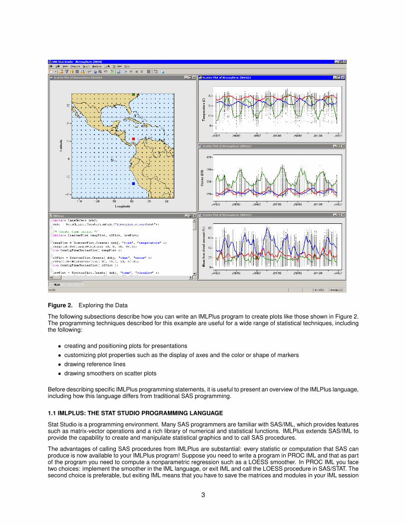
Figure 2. Exploring the Data

The following subsections describe how you can write an IMLPlus program to create plots like those shown in Figure 2.The programming techniques described for this example are useful for a wide range of statistical techniques, includingthe following:

• creating and positioning plots for presentations• customizing plot properties such as the display of axes and the color or shape of markers• drawing reference lines• drawing smoothers on scatter plots

Before describing specific IMLPlus programming statements, it is useful to present an overview of the IMLPlus language,including how this language differs from traditional SAS programming.

1.1 IMLPLUS: THE STAT STUDIO PROGRAMMING LANGUAGE

Stat Studio is a programming environment. Many SAS programmers are familiar with SAS/IML, which provides featuressuch as matrix-vector operations and a rich library of numerical and statistical functions. IMLPlus extends SAS/IML toprovide the capability to create and manipulate statistical graphics and to call SAS procedures.

The advantages of calling SAS procedures from IMLPlus are substantial: every statistic or computation that SAS canproduce is now available to your IMLPlus program! Suppose you need to write a program in PROC IML and that as partof the program you need to compute a nonparametric regression such as a LOESS smoother. In PROC IML you facetwo choices: implement the smoother in the IML language, or exit IML and call the LOESS procedure in SAS/STAT. Thesecond choice is preferable, but exiting IML means that you have to save the matrices and modules in your IML session

3

(by using the STORE statement), call the LOESS procedure, reload the previous IML session, and then continue on.If you forget to use the STORE statement, your IML results are gone. In IMLPlus, you can call procedures and DATAsteps as if they were built-in functions. All IMLPlus graphs, matrices, and modules continue to persist when you call aSAS procedure.

The IMLPlus programming language borrows ideas from object-oriented programming, particularly Java. An object isa variable that refers to a class. The class is a “template” for the object: it specifies the data and the functions (calledmethods) that query, retrieve, and manipulate the data. In IMLPlus, a variable is implicitly assumed to be an IML matrixunless you use the declare keyword to specify that the variable is an object.

To call class methods in IMLPlus, you use a “dot notation” syntax in which the method name is appended to the nameof the object. All IMLPlus methods (and an example of their use) are documented in the Stat Studio online Help. (SelectHelp I Help Topics from the main menu and then expand the topic for “IMLPlus Class Reference.”) The DataObjectand Plot classes contain the most methods. Most classes are derived from base classes. Derived classes can usemethods in their base classes. For example, a ScatterPlot can use methods for the Plot2D class, the Plot class, andthe DataView class. Appendix A lists frequently used IMLPlus methods.

1.2 A SIMPLE IMLPLUS PROGRAM

This section introduces a few elementary IMLPlus programming statements. The emphasis is on the “Plus” portion ofthe language. The goal of this section is to describe how to write an IMLPlus program to create the plot in Figure 2.

In this example, the data are in a SAS data set named Atmospheric.sas7bdat. The data set is located on the PC runningStat Studio, in a directory that Stat Studio automatically searches. The following program shows how to read in the dataand create a scatter plot of Temperature versus Time:

declare DataObject dobj; /* class to manage data */dobj = DataObject.CreateFromFile("Atmospheric.sas7bdat"); /* data set on PC */

declare ScatterPlot tempPlot; /* scatter plot class */tempPlot = ScatterPlot.Create( dobj, "time", "temperature" );

The first statement in the program specifies that dobj is an object of the DataObject class. The next statement creates(or instantiates) the object with the data from the Atmospheric data set. The dobj variable contains an in-memory copyof the data. It manages graphical information about observations, such as the shape and color of markers, whetheran observation is selected, and so forth. The fact that the data resides in memory is important: it enables the highlyinteractive linking between plots.

The two subsequent statements create a scatter plot. Because the scatter plot is created from a DataObject, it isautomatically linked to any other graphical or tabular view that is created from the same DataObject. For example, thescatter plots and data table in Figure 1 are linked because they share a common DataObject.

You can change attributes of a plot programmatically, or you can change them interactively by using the Stat Studio GUI.For example, on the time series plot for temperature you might want to show a variable’s label instead of the variable’sname. You also might want to set the tick marks on the time axis to be a multiple of six months, beginning with January.

Because Figure 2 shows three time series plots, it is convenient to define an IMLPlus module that configures anarbitrary plot. You can then call the module for any time series plot. The following statements define a module thattakes a ScatterPlot object as its argument and sets various attributes. (In fact, the module could be defined to acceptany object of the Plot class.)

start ConfigureTimeSeriesPlot( ScatterPlot plot );plot.SetAxisLabel(YAXIS,AXISLABEL_VARLABEL); /* show variable label */plot.SetAxisLabel(XAXIS,AXISLABEL_VARLABEL); /* instead of name */plot.SetAxisTickAnchor(XAXIS, ’16JAN1995’d );/* set first tick */plot.SetAxisTickUnit(XAXIS, 365 ); /* 365 days between ticks */plot.SetAxisMinorTicks(XAXIS, 1 ); /* minor tick (6 months) */

finish;

You can call this module as shown in the following statement:

run ConfigureTimeSeriesPlot( tempPlot );

4

The resulting time series plot is shown in Figure 3. Similar statements create and configure the time series plots forOzone and CloudLow in Figure 2.

Figure 3. Adjusted Time Series Plot

1.3 OVERLAYING INFORMATION ON A PLOT

This section describes how to draw curves and polygons on plots. Although the example of this section overlays a mapon the scatter plot of spatial positions shown in Figure 2, the ideas of this section apply to drawing a wide range ofstatistical concepts, including the following:

• reference lines

• density estimates on a histogram

• regression curves on a fit plot

• confidence ellipses for bivariate density on a scatter plot

The IMLPlus programming language provides a large number of methods to draw lines, curves, markers, polygons, andtext on a plot. You can define your own coordinate system or use the coordinate system defined by the data. Thesemethods all begin with the prefix “Draw” so that they are easy to find in the Stat Studio documentation.

For example, to draw a map in the background of the scatter plot of spatial locations, you can use the DrawPolygonsmethod. (A map data set, as used by GMAP procedure in SAS/GRAPH , consists of a series of polygons. You candownload map data sets that specify the boundaries of many countries at support.sas.com.) Since country boundariesare often defined in a map data set, Stat Studio distributes an IMLPlus module called DrawPolygonsByGroups thatreads a map data set and provides several convenient methods for coloring the polygons.

The following statements create a scatter plot of spatial positions and reposition the plot. The plot is passed into amodule called DrawMap which colors the background of the scatter plot blue (so that it looks like water), draws thecountries of North, Central, and South America, and adds reference lines at certain latitudes to represent the Tropic ofCancer and the Equator.

5

declare ScatterPlot spatialPlot;spatialPlot = ScatterPlot.Create( dobj, "Longitude", "Latitude" );spatialPlot.SetWindowPosition(0,0,50,67 );run DrawMap( spatialPlot );

start DrawMap( ScatterPlot plot );plot.SetPlotAreaBackgroundColor(215,235,255); /* light blue */plot.SetPlotAreaMargins(0.01, 0.01, 0.01, 0.01);plot.SetGraphAreaMargins(0.15, 0.15, 0.1, 0.1);

plot.DrawSetRegion(PLOTBACKGROUND);plot.DrawUseDataCoordinates();

declare DataObject dobjMap;dobjMap = DataObject.CreateFromFile( "Maps\NSAmerica.sas7bdat" );run DrawPolygonsByGroups( plot, dobjMap, "Longitude", "Latitude",

{"ID" "Segment"}, "Uniform", CREAM//BLACK, true );

plot.DrawSetPenColor( GREY );plot.DrawLine( -120, 0, 0, 0 ); /* Equator */plot.DrawLine( -120, 23.5, 0, 23.5 ); /* Tropic of Cancer */

finish;

Figure 4 shows the resulting scatter plot, with a spatial location near SAS World Headquarters highlighted. Note thatthe plot is created by using the same DataObject used to create the time series plot. This causes the plots to be linkedto each other. By using the two plots together, it is much easier to investigate how geographic and climatic featuressuch as oceans, deserts, mountains, and rain forests affect the atmospheric variables.

You can use IMLPlus drawing methods to overlay any Stat Studio plot with curves or polygons. For instance, you canadd density estimates to histograms or smoothers to scatter plots. You can use the DrawPolygons method to drawconfidence ellipses for the mean of bivariate data. You can also draw markers and text on plots to indicate outliers orinfluential observations.

Figure 4. Overlaying a Map and a Scatter Plot

6

1.4 ACTION MENUS: RESPONDING TO USER INTERACTIONS

By interacting with Stat Studio’s graphics, it is easy to select subsets of data that have certain properties. For example,you can select all data for spatial positions near the equator by clicking in a histogram of Latitude. You might decide toperform an analysis for only a selected subset of data. This section shows how you can write an IMLPlus module thatexamines the currently selected observations and performs an analysis only for the selected data.

Stat Studio enables you to attach a menu, called an action menu, to a plot. When you select the menu item, StatStudio executes IMLPlus code that you specify. Consequently, you can write IMLPlus code that examines the currentlyselected observations and performs an action based on those observations.

The following statements specify a simple module that can be called by an action menu attached to any plot. Forillustration, the module is attached to a time series plot described in the previous section.

tempPlot.AppendActionMenuItem( "Print number of selected observations","run OnActionMenu();" );

start OnActionMenu();declare Plot plot = Plot.GetInitiator(); /* get action menu owner */declare DataObject dobj = plot.GetDataObject();/* get plot’s DataObject */dobj.GetSelectedObsNumbers( SelObsIdx );print "There are " (nrow(SelObsIdx)) "selected observations";

finish;

When you run the program that contains this code, the AppendActionMenuItem method attaches a menu to the scatterplot. You can display the menu by pressing the F11 key. The menu contains one item, labeled “Print number of selectedobservations.” When you select that item, Stat Studio calls the OnActionMenu module.

When the module executes, it calls the GetInitiator method in the Plot class. This method returns a reference to thePlot object to which the action menu is attached. The subsequent statement gets the DataObject connected to the plot.The module then queries the DataObject for the selected observations and uses IML to print how many observationsare selected.

This simple example can be extended to one that draws lines that connect the monthly averages of each selectedspatial position. (As noted earlier, if you select two or more spatial positions in Figure 1, it is difficult to discern whichtime series is associated with each spatial location.) The following statements define an action menu that calls a modulethat draws the lines shown in Figure 2.

7

tempPlot.AppendActionMenuItem( "Trace selected observations","run OnMenuTraceSelectedTimeSeries();" );

start OnMenuTraceSelectedTimeSeries();declare Plot plot = Plot.GetInitiator(); /* get action menu owner */plot.DrawRemoveCommands("TraceSelectedTimeSeries");/* remove previous lines */

declare DataObject dobj = plot.GetDataObject();/* get plot’s DataObject */dobj.GetSelectedObsNumbers( SelObsIdx );if ncol(SelObsIdx)=0 then

return;

dobj.GetVarData("SpatialPosition", Pos); /* 1 */SelPos = unique( Pos[SelObsIdx] ); /* 2 */dobj.GetVarData("time", T);plot.GetVars(ROLE_Y, yVarName); /* name of Y variable */dobj.GetVarData(yVarName, Y);

plot.DrawBeginBlock("TraceSelectedTimeSeries");plot.DrawUseDataCoordinates();plot.DrawSetPenWidth(2);do k = 1 to ncol(SelPos);

idx = loc( Pos = SelPos[k] ); /* 3 */plot.DrawLine(T[idx], Y[idx]); /* 4 */print yVarName "Position=" (SelPos[k]) "mean=" (Y[idx][:]); /* 5 */

end;plot.DrawEndBlock();

finish;

The module uses a pair of IMLPlus methods (DrawBeginBlock, DrawEndBlock) to associate a group of drawing com-mands with a name (in this case, “TraceSelectedTimeSeries”). All of the commands in the group can be removed bycalling the DrawRemoveCommands method. Consequently, when this module is called a second time, the moduleerases any lines that it previously drew. Then the module draws a new set of lines.

The module performs the following operations:

1. The entire SpatialPosition variable is retrieved from the DataObject into an IML vector called Pos.

2. The IML UNIQUE function determines which spatial positions are selected.

3. Within the IML loop, all (t, y) pairs for the selected positions are extracted by using the IML LOC function andstandard IML index operators.

4. The DrawLine method is used to draw a series of line segments that connect the time series for the selectedpositions. (This assumes the data are sorted by time.)

5. The mean value of the time series is printed.

You can include additional statements that change the color of each line. Figure 5 shows the action menu and theresulting lines that connect each time series for the three spatial locations highlighted in Figure 2.

8

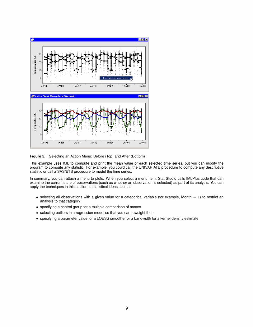
Figure 5. Selecting an Action Menu: Before (Top) and After (Bottom)

This example uses IML to compute and print the mean value of each selected time series, but you can modify theprogram to compute any statistic. For example, you could call the UNIVARIATE procedure to compute any descriptivestatistic or call a SAS/ETS procedure to model the time series.

In summary, you can attach a menu to plots. When you select a menu item, Stat Studio calls IMLPlus code that canexamine the current state of observations (such as whether an observation is selected) as part of its analysis. You canapply the techniques in this section to statistical ideas such as

• selecting all observations with a given value for a categorical variable (for example, Month = 1) to restrict ananalysis to that category

• specifying a control group for a multiple comparison of means

• selecting outliers in a regression model so that you can reweight them

• specifying a parameter value for a LOESS smoother or a bandwidth for a kernel density estimate

9

2. BUILDING STATISTICAL MODELS

You can explore data by using the Stat Studio GUI to discover relationships between variables. After a relationship isdiscovered, you might choose to build a statistical model for this relationship.

A scatter plot of Ozone by Latitude (all observations in Figure 6) suggests that atmospheric ozone might be quadraticallyrelated to latitude. However, interactive exploration of the data suggests that the relationship depends on the monthof the year, suggesting an interaction effect between latitude and month. For example, the highlighted observationsin Figure 6 show the relationship for all locations during the month of September (Month = 9) for all years. (Recallthat there are six years of data.) Consequently, any model of ozone should include an interaction between Month andLatitude.

Figure 6. Relationship between Ozone and Latitude (September Measurements Plotted in Color)

Stat Studio has a GUI interface to the GENMOD procedure that enables you to analyze linear models of these datawithout writing a program. However, suppose you are interested in modeling these data by using a procedure that isnot built into Stat Studio. For example, you might want to model the conditional quantiles of these data by using theQUANTREG procedure. The following statements show how you can call a SAS procedure, read the results into IMLmatrices, and draw predicted values on the scatter plot in Figure 6.

10

/* write a subset of variables to WORK data set */vars = { "MonthNum" "Month" "Latitude" "Ozone"};dobj.WriteVarsToServerDataSet( vars, "Work", "Ozone", true );

submit;proc quantreg data=Ozone CI=NONE;

class Month;/* "bar operator" generates interaction effects */model Ozone = Month | Latitude | Latitude*Latitude / quantiles=0.25 0.5 0.75;output out=QuantOut Pred=Pred_Ozone;

run;endsubmit;

/* Plot Ozone versus Latitude */declare ScatterPlot o3Plot;o3Plot = ScatterPlot.Create( dobj, "Latitude", "Ozone" );o3Plot.SetTitleText("Quantile Regression for Months 3 and 9");o3Plot.ShowTitle();

/* Read certain predicted quantiles from output data set */months = {3 9};colors = BLUE || RED;

use QuantOut where(MonthNum<=12 & Month=months);read all var {Month Latitude Pred_Ozone1 Pred_Ozone2 Pred_Ozone3};close QuantOut;

o3Plot.DrawUseDataCoordinates();do i = 1 to ncol(months);

idx = loc( Month = months[i] );o3Plot.DrawSetPenColor( colors[i] );o3Plot.DrawLine( Latitude[idx], Pred_Ozone1[idx] );o3Plot.DrawLine( Latitude[idx], Pred_Ozone2[idx] );o3Plot.DrawLine( Latitude[idx], Pred_Ozone3[idx] );

end;

The previous program statements write a subset of the atmospheric data to the WORK library so that the QUANTREGprocedure can access the relevant variables. The QUANTREG procedure can be called within a SUBMIT/ENDSUBMITblock. All statements within the block are sent to SAS. Note that this step is impossible in traditional IML, since callinga procedure causes PROC IML to exit. In contrast, IMLPlus can call a SAS procedure and also preserve all plots andvariables.

The program creates a scatter plot of ozone versus latitude and uses standard IML statements to read certain predictedquantiles from the output data set into matrices. These quantile values are plotted on the scatter plot shown in Figure 7.Note that the program used a WHERE clause to read and display only the predicted 25th, 50th, and 75th percentiles forMarch (Month = 3, displayed in blue) and September (Month = 9, displayed in red). With a few additional statements,you can add a legend by calling the DrawLegend module that is distributed with Stat Studio.

11

Figure 7. Partial Results of Quantile Regression

3. ADVANCED PROGRAMMING TECHNIQUES

Stat Studio provides the following features that enable you to program techniques that might be difficult to implementby using other software:

• A program can pass values from IMLPlus into SAS by specifying the names of matrices in the SUBMIT statement.SAS procedures can access these values as if they were macro variables.

• A program can display dialog boxes to query for user input. For example, the DoDialogGetListItems moduleenables you to choose one or more items from a list.

• The PAUSE statement causes a program to pause while the user selects observations or otherwise interacts withthe data. Upon resuming execution, the program can incorporate the user’s selections into the analysis.

• A program can attach menu items to a plot or data table, as described earlier in this paper.

• A program can animate plots to display results that vary according to a tuning parameter. This is discussedfurther in the next subsection.

• Stat Studio supports running programs simultaneously in multiple workspaces, with each program running ona different SAS server. Consequently, you can run IMLPlus programs that distribute computing across multipleservers.

A complete description of these techniques is beyond the scope of this paper. However, the next two analyses illustratethe types of techniques that are possible in Stat Studio.

3.1 ANIMATION TECHNIQUES

There are two ways to produce animated graphics in Stat Studio. One way is to sequentially change attributes of thedata. For example, a program can contain a loop that changes the observations that are included in plots or changesthe shape or color of markers. The plots will update accordingly.

A second way is to draw and erase curves or other figures on a plot by using IMLPlus drawing methods (primarilyDrawBeginBlock, DrawEndBlock, and DrawRemoveCommands). This technique is an extension of the ideas presentedin the subsection Action Menus: Responding to User Interactions. Conceptually, a program that uses this techniquesto animate has the following structure:

12

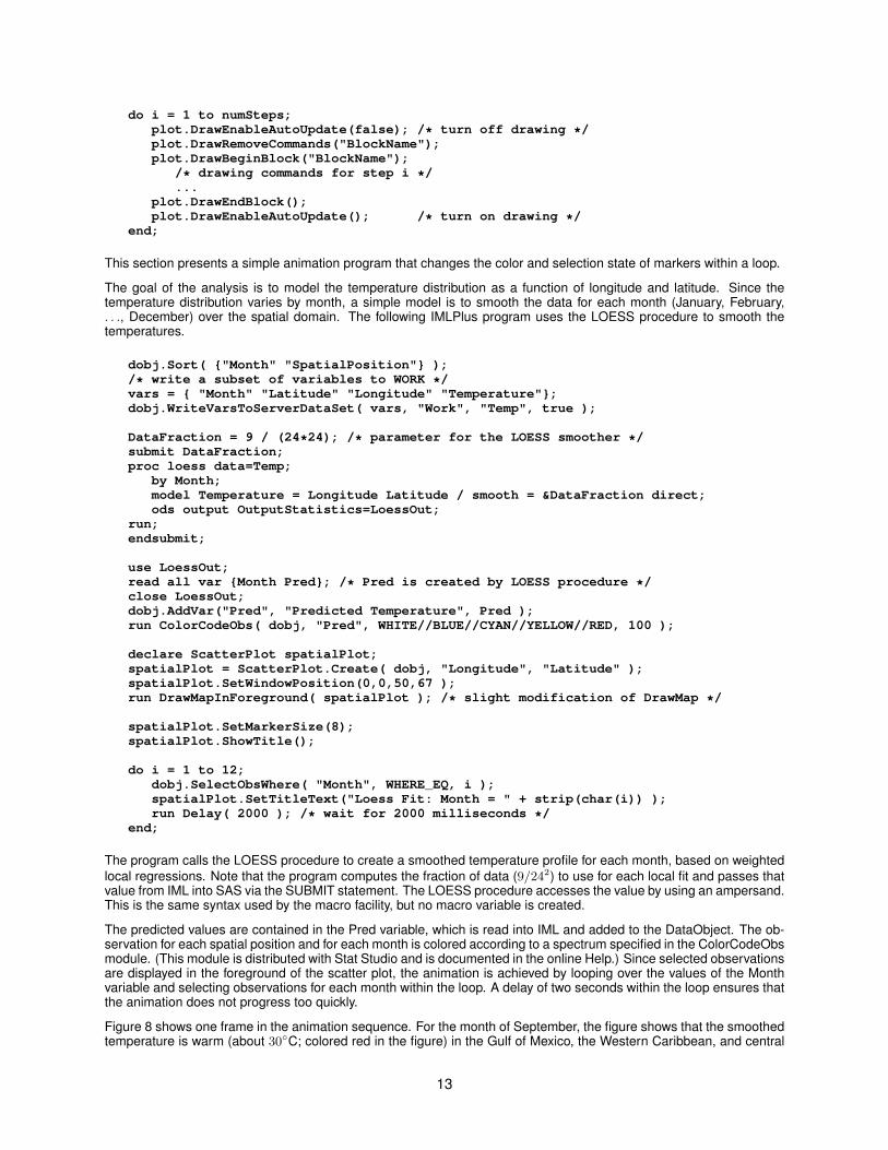
do i = 1 to numSteps;plot.DrawEnableAutoUpdate(false); /* turn off drawing */plot.DrawRemoveCommands("BlockName");plot.DrawBeginBlock("BlockName");

/* drawing commands for step i */...

plot.DrawEndBlock();plot.DrawEnableAutoUpdate(); /* turn on drawing */

end;

This section presents a simple animation program that changes the color and selection state of markers within a loop.

The goal of the analysis is to model the temperature distribution as a function of longitude and latitude. Since thetemperature distribution varies by month, a simple model is to smooth the data for each month (January, February,. . ., December) over the spatial domain. The following IMLPlus program uses the LOESS procedure to smooth thetemperatures.

dobj.Sort( {"Month" "SpatialPosition"} );/* write a subset of variables to WORK */vars = { "Month" "Latitude" "Longitude" "Temperature"};dobj.WriteVarsToServerDataSet( vars, "Work", "Temp", true );

DataFraction = 9 / (24*24); /* parameter for the LOESS smoother */submit DataFraction;proc loess data=Temp;

by Month;model Temperature = Longitude Latitude / smooth = &DataFraction direct;ods output OutputStatistics=LoessOut;

run;endsubmit;

use LoessOut;read all var {Month Pred}; /* Pred is created by LOESS procedure */close LoessOut;dobj.AddVar("Pred", "Predicted Temperature", Pred );run ColorCodeObs( dobj, "Pred", WHITE//BLUE//CYAN//YELLOW//RED, 100 );

declare ScatterPlot spatialPlot;spatialPlot = ScatterPlot.Create( dobj, "Longitude", "Latitude" );spatialPlot.SetWindowPosition(0,0,50,67 );run DrawMapInForeground( spatialPlot ); /* slight modification of DrawMap */

spatialPlot.SetMarkerSize(8);spatialPlot.ShowTitle();

do i = 1 to 12;dobj.SelectObsWhere( "Month", WHERE_EQ, i );spatialPlot.SetTitleText("Loess Fit: Month = " + strip(char(i)) );run Delay( 2000 ); /* wait for 2000 milliseconds */

end;

The program calls the LOESS procedure to create a smoothed temperature profile for each month, based on weightedlocal regressions. Note that the program computes the fraction of data (9/242) to use for each local fit and passes thatvalue from IML into SAS via the SUBMIT statement. The LOESS procedure accesses the value by using an ampersand.This is the same syntax used by the macro facility, but no macro variable is created.

The predicted values are contained in the Pred variable, which is read into IML and added to the DataObject. The ob-servation for each spatial position and for each month is colored according to a spectrum specified in the ColorCodeObsmodule. (This module is distributed with Stat Studio and is documented in the online Help.) Since selected observationsare displayed in the foreground of the scatter plot, the animation is achieved by looping over the values of the Monthvariable and selecting observations for each month within the loop. A delay of two seconds within the loop ensures thatthe animation does not progress too quickly.

Figure 8 shows one frame in the animation sequence. For the month of September, the figure shows that the smoothedtemperature is warm (about 30◦C; colored red in the figure) in the Gulf of Mexico, the Western Caribbean, and central

13

South America. The Peruvian and Chilean Andes exhibit the coldest temperatures (about 10◦C; colored dark blue inthe figure). The cold Humboldt Current, which flows from Antarctica up the coast of Chile and Peru, is visible in thePacific ocean as a cyan-colored area of 17–18◦C temperature.

Figure 8. Animating a Loess Smoother of Temperature by Month

3.2 BOOTSTRAP METHODS

Stat Studio is a natural environment for modern statistical methods such as the bootstrap. You can use bootstrapmethods to estimate the standard error for a statistic or confidence intervals for a parameter. Implementing a bootstrapestimate requires three main steps:

1. Compute the statistic of interest on the original data.

2. Resample B times from the data to form B bootstrap samples.

3. Compute the statistic on each resample.

The statistics computed from the resampled data form a bootstrap distribution for the statistic computed on the originaldata. The bootstrap distribution is an estimate for the distribution of the statistic. In particular, the standard deviation ofthe bootstrap distribution is an estimate for the standard error of the statistic. Percentiles of the bootstrap distributionare the simplest estimate for confidence intervals.

Resampling from data that are temporally or spatially correlated requires advanced resampling techniques that arebeyond the scope of this article (see chapter 8 of Davison and Hinkley, 1997). The remainder of this section uses onlydata for SpatialPosition = 15 during the summer months (June, July, and August).

The starting point for the bootstrap example is a principal component analysis for the variables Temperature, Ozone,Pressure, CloudLow, CloudMid, and CloudHigh. Figure 9 shows the proportion of variance in the data explained byeach principal component, as computed by the PRINCOMP procedure.

14

Figure 9. Eigenvalues of the Correlation Matrix

Let Pi be the proportion of variance explained by the ith principal component, i = 1 . . . 6. According to the table, thefirst principal component explains 42.1% of the variance. But how much uncertainty is in that estimate? Is a 90%confidence interval for the proportion of variance small (such as [0.42, 0.422]) or large (such as [0.32, 0.52])? Thereis no analytic formula for estimating the confidence interval, but bootstrap methods provide a computational way toestimate the distribution of P1, and, in fact, any of the Pi.

The following program computes Figure 9 and determines how many principal components explain more than 10% ofthe variance in the data.

declare DataObject dobj;dobj = DataObject.CreateFromFile("Atmospheric.sas7bdat");VarNames = {"Temperature" "Ozone" "Pressure" "CloudLow" "CloudMid" "CloudHigh"};WhereNames = {"SpatialPosition" "Month"};

/* Write a subset of data to WORK */dobj.WriteVarsToServerDataSet( VarNames||WhereNames, "Work", "_BootIn", true );

submit VarNames;data _BootIn;set _BootIn(where=(SpatialPosition=15 & Month in (6,7,8)));run;

/* Compute statistic (proportion of variance explained by PC) */proc princomp data=_BootIn;

var &VarNames;ods output Eigenvalues=DataEVals;ods exclude Eigenvectors;

run;endsubmit;

use DataEVals; read all var {Proportion}; close DataEVals;N = ncol( loc(Proportion >= 0.1) ); /* choose PCs that explain >= 10% */

The program writes a subset of the variables to WORK. The DATA step uses a WHERE clause to subset the obser-vations. (It is also possible for the DataObject to write only a subset of observations.) The PRINCOMP procedurecomputes and saves the statistics (shown in Figure 9) for the original data. The statistics are read into an IML vector,and IML is used to dynamically compute the number of principal components (N = 3) that explain at least 10% of thevariance.

The remainder of the program implements a bootstrap algorithm to estimate the 90% confidence intervals for theProportion statistic:

15

B = 1000; /* number of bootstrap samples */

submit B N VarNames;/* Resample data B times (sampling with replacement) */proc surveyselect data=_BootIn NOPRINT

method=urs samprate=1 rep=&B out=_Resample;run;

/* Compute the statistic for each bootstrap sample */ods listing exclude all;proc princomp data=_Resample N=&N;

by Replicate;freq NumberHits;var &VarNames;ods output Eigenvalues=BootEVals(drop=eigenvalue difference cumulative);

run;ods listing exclude none;

proc datasets nolist; delete _: ; run; /* delete temporary data sets */

/* Transpose results for easy graphing */proc transpose data=BootEvals out=BootEvals prefix=Proportion;

by Replicate;var Proportions;

run;

/* Compute mean and percentiles of bootstrap distribution */proc means data=BootEvals N Mean StdDev P5 P95;

var Proportion: ;run;endsubmit;

The SURVEYSELECT procedure creates bootstrap samples by sampling with replacement from the data. The OUT=data set created by SURVEYSELECT includes the Replicate variable, an indicator variable with values 1 . . . B. ThePRINCOMP procedure computes the Pi statistics on each resample by using Replicate as a BY variable. See Cassel(2007) for more details about using SURVEYSELECT for bootstrapping.

The MEANS procedure summarizes the bootstrap distributions of the Pi, as shown in Table 1. The results indicate that,with 90% confidence, the first principal component explains between 32.7% and 57.1% of the variance. Accordingly,you can conclude that the estimate of P1 has large uncertainty for these data.

Table 1. Descriptive Statistics for the Bootstrap DistributionsVariable Mean Std Dev 5th Pctl 95th PctlProportion1 0.4494165 0.0733330 0.3277346 0.5712238Proportion2 0.2491871 0.0346577 0.1905428 0.3062375Proportion3 0.1425635 0.0333312 0.0886981 0.1982759

The program can be extended by reading these descriptive statistics into IMLPlus and graphically displaying thesevalues on histograms that show the bootstrap distributions for the Pi, as shown in Figure 10.

16

Figure 10. Bootstrap Distributions of Proportions

Note the value added by using Stat Studio. In addition to calling SAS procedures as if they were IML functions, and inaddition to being able to pass data from IML into procedures, Stat Studio enables you to dynamically examine the jointbootstrap distributions. In Figure 10, values in the lower tail of P1 are selected. The corresponding marginal distributionof P3 values are shifted to the right. This makes sense because the sum of the proportions is unity. This is a powerfulmechanism for understanding relationships between bootstrap distributions.

CONCLUSIONS

Stat Studio is a programming environment for high-end data analysts. The Stat Studio language, IMLPlus, blends thestrengths of IML and SAS programming, while introducing new classes and methods for creating and manipulatingdynamically linked graphics. The interactive graphics facilitate building statistical models because you can readilydiscover relationships between variables.

Stat Studio enables you to program sophisticated analyses by using IML and by calling SAS procedures as functions.You can visualize the results with linked graphics. Advanced techniques described in this paper include animation andthe bootstrap method. The examples in this paper used time series and spatial data, but the Stat Studio techniquesdescribed in this paper are generally applicable to a wide range of statistical analyses.

17

APPENDIX A: FREQUENTLY USED IMLPLUS METHODS

Some IMLPlus methods are used more frequently than others. The following tables list several classes and frequentlyused methods in each of those classes. You can access the documentation for these methods (with examples ofusage) by selecting Help I Help Topics from the Stat Studio main menu. The documentation is in the “IMLPlus ClassReference” chapter of SAS Stat Studio Help.

Table 2. DataObject Class MethodsAddVar IsNominalCreateFromFile IsNumericCreateFromServerDataSet SelectObsGetNumObs SelectObsWhereGetSelectedObsNumbers SetMarkerColorGetVarData SetMarkerShapeIncludeInAnalysis SortIncludeInPlots WriteVarsToServerDataSet

Table 3. DataView Class MethodsActivateWindow GetInitiatorAppendActionMenuItem SetWindowPositionGetDataObject ShowWindow

Table 4. Plot Class MethodsCopyToOutputDocument GetVarsDrawBeginBlock SetAxisNumericTicksDrawEndBlock SetGraphAreaMargins (Plot2D class)DrawLine SetMarkerSizeDrawMarker SetObsLabelVarDrawRemoveComands SetPlotAreaMarginsDrawSetPenColor SetTitleTextDrawSetBrushColor ShowObsDrawText ShowReferenceLinesDrawUseDataCoordinates ShowTitle

In addition to IMLPlus methods, Stat Studio is distributed with a number of useful modules. The module documentationis in the “IMLPlus Module Reference” chapter. The following table lists frequently used modules:

Table 5. IMLPlus ModulesColorCodeObs DoDialogModifyDoubleColorCodeObsByGroups DoMessageBoxYesNoCopyServerDataToDataObject DrawInsetDelay DrawLegendDoDialogGetListItems GetPersonalFilesDirectory

Lastly, some IML statements have enhanced functionality in IMLPlus. The “The IMLPlus Language” chapter documentsthese enhancements. These include the following features:

• You can call SAS procedures as functions by using the SUBMIT/ENDSUBMIT statements.

• You can pause a program to interact with the data by using the PAUSE statement.

• You can pass any Java class as an argument to an IMLPlus module.

• You can use matrix expressions with the CREATE, USE, and CLOSE statements.

18

REFERENCES

American Statistical Association (2006). “Data Exposition 2006.” The data are available at www.amstat-online.org/sections/graphics/dataexpo/2006.php.

Cassell, D. L. (2007), “Don’t Be Loopy: Re-Sampling and Simulation the SAS Way,” Proceedings of the SAS GlobalForum 2007 Conference. Cary, NC: SAS Institute Inc.

Davison, A. C., and Hinkley, D. V. (1997), Bootstrap Methods and Their Application. Cambridge, UK: CambridgeUniversity Press.

Wicklin, R., and Rowe, P. (2007), “An Introduction to SAS Stat Studio: A Programmable Successor to SAS/INSIGHT,”Proceedings of the SAS Global Forum 2007 Conference. Cary, NC: SAS Institute Inc.

CONTACT INFORMATION

Rick WicklinSAS Institute Inc.SAS Campus DriveCary, NC 27513www.sas.com/statistics

SAS and all other SAS Institute Inc. product or service names are registered trademarks or trademarks of SAS InstituteInc. in the USA and other countries. R© indicates USA registration.

Other brand and product names are trademarks of their respective companies.

19