Dillards 2016 Data Extraction

Created June 2018

Create by Ron Freeze – June 2018

SAS Enterprise Guide Summary Analytics & Hypothesis Testing

(June, 2018)

Sources (adapted with permission)-

Ron Freeze Course and Classroom Notes

Enterprise Systems, Sam M. Walton College of Business, University of Arkansas, Fayetteville

SAS® Multivariate Statistics Course Notes & Workshop, 2010

SAS® Advanced Business Analytics Course Notes & Workshop, 2010

Teradata® University Network

Copyright © 2013 ISYS 5503 Decision Support and Analytics, Information Systems; Timothy Paul

Cronan. For educational uses only - adapted from sources with permission. No part of this publication

may be reproduced, stored in a retrieval system, or transmitted, in any form or by any means, electronic,

mechanical, photocopying, or otherwise, without the prior written permission from the author/presenter.

2

Create by Ron Freeze – June 2018

Here’s the Story…

This tutorial walks you through features and functions of SAS Enterprise Guide 7.1. The basis of this

tutorial is a data set from Dillards that was extracted from the University of Arkansas Enterprise Systems

group in the Information Systems Department. There are two exercises that include: 1) summary statistics

for the Midwest Area (AR, KS, MO, OK) Sales Revenue, and 2) a hypothesis test determining the stores

that are statistically different in sales from the State average. The focus of this analysis will be Sales

Revenue for the year 2015.

NOTE: Use of this tutorial requires access to SAS Enterprise Guide 7. Obtaining the data for this tutorial

requires an extracted Dillards 2016 file from the Enterprise Systems at the University of Arkansas

(https://walton.uark.edu/enterprise/). The data is extracted using the file “Dillards 2016 Data Extraction-

TUNtoExcel-KPIs.pdf” (available on the Enterprise Systems website and the Teradata University

Network website) and should not be downloaded to your personal drives. The file should remain on the

Remote Desktop S: drive provided by the University of Arkansas. This is due to our agreement with the

data providers. Questions can be directed to Ron Freeze at rfreeze@walton.uark.edu.

ESTIMATED COMPLETION TIME: 20-40 minutes

Connect to your data

The following section is duplicated from the Pre-Conference Preparation.docx document for connecting

to your data. The end result is a project file (.egp) that has the data already identified for this tutorial. If

this has been accomplished, please skip to Create Summary Statistics.

Verify SAS-EG Access and set up project file

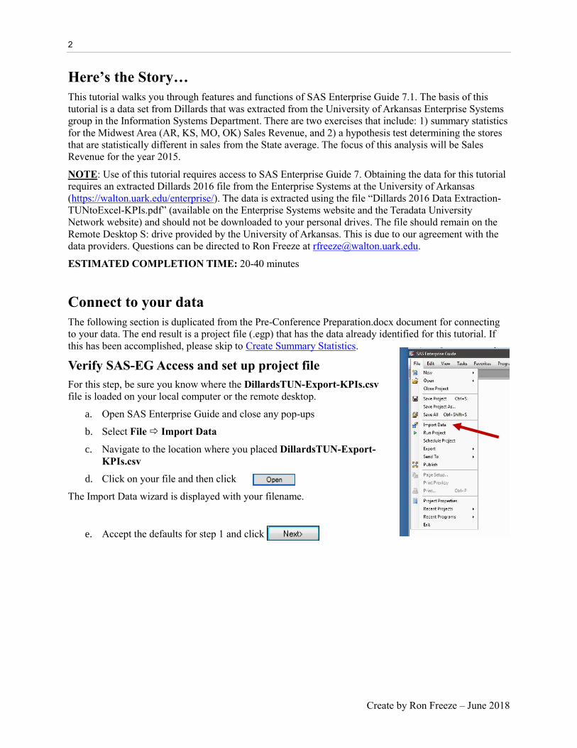
For this step, be sure you know where the DillardsTUN-Export-KPIs.csv

file is loaded on your local computer or the remote desktop.

a. Open SAS Enterprise Guide and close any pop-ups

b. Select File Import Data

c. Navigate to the location where you placed DillardsTUN-Export-

KPIs.csv

d. Click on your file and then click

The Import Data wizard is displayed with your filename.

e. Accept the defaults for step 1 and click

3

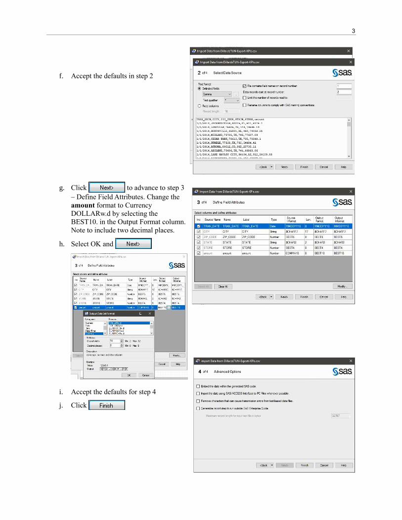
f. Accept the defaults in step 2

g. Click to advance to step 3

– Define Field Attributes. Change the

amount format to Currency

DOLLARw.d by selecting the

BEST10. in the Output Format column.

Note to include two decimal places.

h. Select OK and

i. Accept the defaults for step 4

j. Click

4

Create by Ron Freeze – June 2018

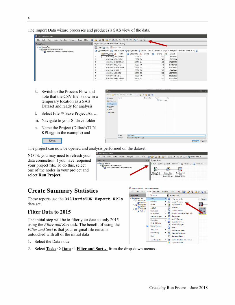
The Import Data wizard processes and produces a SAS view of the data.

k. Switch to the Process Flow and

note that the CSV file is now in a

temporary location as a SAS

Dataset and ready for analysis

l. Select File Save Project As….

m. Navigate to your S: drive folder

n. Name the Project (DillardsTUN-

KPI.egp in the example) and

The project can now be opened and analysis performed on the dataset.

NOTE: you may need to refresh your

data connection if you have reopened

your project file. To do this, select

one of the nodes in your project and

select Run Project.

Create Summary Statistics

These reports use the DillardsTUN-Export-KPIs

data set.

Filter Data to 2015

The initial step will be to filter your data to only 2015

using the Filter and Sort task. The benefit of using the

Filter and Sort is that your original file remains

untouched with all of the initial data

1. Select the Data node

2. Select Tasks Data Filter and Sort… from the drop-down menus.

5

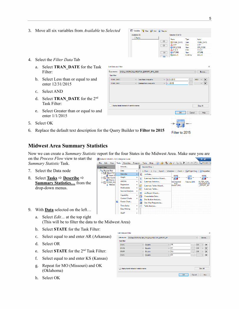
3. Move all six variables from Available to Selected

4. Select the Filter Data Tab

a. Select TRAN_DATE for the Task

Filter:

b. Select Less than or equal to and

enter 12/31/2015

c. Select AND

d. Select TRAN_DATE for the 2nd

Task Filter:

e. Select Greater than or equal to and

enter 1/1/2015

5. Select OK

6. Replace the default text description for the Query Builder to Filter to 2015

Midwest Area Summary Statistics

Now we can create a Summary Statistic report for the four States in the Midwest Area. Make sure you are

on the Process Flow view to start the

Summary Statistic Task.

7. Select the Data node

8. Select Tasks Describe

Summary Statistics… from the

drop-down menus.

9. With Data selected on the left…

a. Select Edit… at the top right

(This will be to filter the data to the Midwest Area)

b. Select STATE for the Task Filter:

c. Select equal to and enter AR (Arkansas)

d. Select OR

e. Select STATE for the 2nd Task Filter:

f. Select equal to and enter KS (Kansas)

g. Repeat for MO (Missouri) and OK

(Oklahoma)

h. Select OK

6

Create by Ron Freeze – June 2018

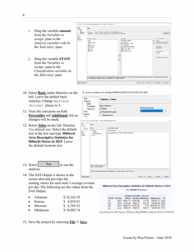
i. Drag the variable amount

from the Variables to

assign: pane to the

Analysis variables role in

the Task roles: pane.

j. Drag the variable STATE

from the Variables to

assign: pane to the

Classification variables in

the Task roles: pane

10. Select Basic under Statistics on the

left. Leave the default basic

statistics. Change Maximum

decimal places to 2.

11. View the selections on both

Percentiles and Additional, but no

changes will be made.

12. Select Titles on the left. Deselect

Use default text. Select the default

text in the box and type Midwest

Area Descriptive Statistics for

Dillards Stores in 2015. Leave

the default footnote text.

13. Select to run the

analysis.

14. The SAS Output is shown in the

screen shot and provides the

starting values for each state’s average revenue

per day. The following are the values from the

SAS Output.

Arkansas $ 32,242.55

Kansas $ 8,854.01

Missouri $ 6,705.22

Oklahoma $ 10,085.74

15. Save the project by selecting File Save

7

Summary Statistics on your own

Midwest Area Stores per State

Add the variable store as a Classification variable in order

to see the Summary Statistics for each store. The screen

shot is the SAS Output of this modification. Then means of

each store will be the comparison’s made in the hypothesis

testing of the next section.

Store Sales Differences

A further investigation of store differences is accomplished with a two-tailed hypothesis test in which we

will first determine if each store is significantly different than the average stores sales. The second step

will be a determination if the store is significantly lower or significantly higher than that states average.

The test is evaluated at the 95% confidence level. The model tested is written as follows for the 10 stores

in Arkansas. NOTE: SAS Enterprise Guide tests each store individually with respect to the mean for the

state.

Ho: $ 32,242.55 = 402 = 403 = 404 = … = 896

HA: At least two daily store revenue sales are not equal

The hypothesis test to answer our question of whether the individual stores are different than the state

mean is considered a Test of

Location. Each store is compared to

the State mean and the Distribution

analysis task is used to determine

the analysis results. We can start

with the Process flow diagram that

we ended with when creating our

Summary Statistics.

1. Select the same filtered SAS

Data set used for the Summary

Statistics

2. Select Tasks Describe Distribution Analysis….

3. Edit the Task Filter to only include AR (Arkansas)

4. Use the amount variable as the analysis variable

5. Use the STORE variable as the Group analysis by

8

Create by Ron Freeze – June 2018

6. Click Tables and…

a. Check the box for Basic

confidence intervals

b. Check the box for Basic

measures

c. Check the box for Tests for

location and then type the value

32,242.55 in the field next to

Null Hypothesis: Ho: Mu=

7. Click Titles and replace the default text with the following: Hypothesis test for Arkansas Stores

Different from the State Average

8. Click Run

9. The 10 hypothesis tests ran result in significance for all of the stores. This translates to a rejection that

any store is at the mean for the state average in Sales Revenue. The individual hypothesis tests will

indicate whether each store is significantly below the state mean or significantly higher than the state

mean. The following are an example of each and include potential questions that should be asked to

address potential additional tests for decision-making.

Stores Performing above Average

Only Store 698 (1 out of 10 stores) exceeded the State

Average daily Revenue in sales ($32,243). Their mean

sales were $ 219,381 compared to the next closest store

(405) at $ 28,146. The positive Students’ t statistic along

with the p-value <.0001 indicates that Store 698 is

significantly higher than the State average. The

following questions may arise from this analysis

Is Store 698 an outlier?

What circumstances contribute to the

performance of Store 698?

Should Store 698 be compared to the other 9

stores in Arkansas?

Stores Performing below Average

Store 405, at $ 28,146 was the best performing store

that was below the State average. The negative

Students’ t statistic along with the p-value <.0001

indicates that Store 698 is significantly lower than the

State average. Part of the purpose to understanding the

differences among store performance is to learn from

the top performing stores and improve the lower

performing stores. With 9 stores below the State

average, the following questions may arise from this

analysis

Should a new “State average” be computed

eliminating Store 698?

9

Which Stores should be differentiated as “best with this new analysis?

Would Standards of performance hold from State to State?

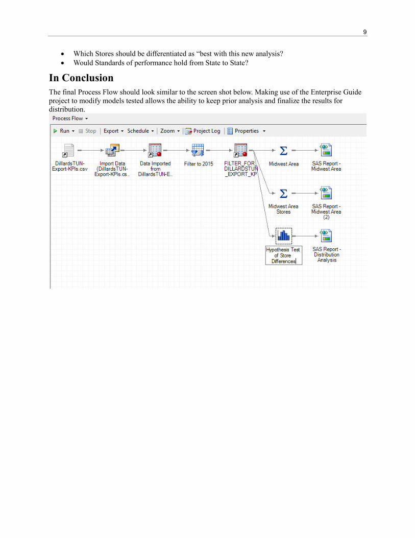
In Conclusion

The final Process Flow should look similar to the screen shot below. Making use of the Enterprise Guide

project to modify models tested allows the ability to keep prior analysis and finalize the results for

distribution.