International Journal of Applied Science and Technology Vol. 2 No. 9; November 2012

40

Sarima Time Series Model Application to Microwave Transmission of Yeji-Salaga

(Ghana) Line-Of-Sight Link

F. K. Oduro-Gyimah

E. Harris

K. F. Darkwah

Department of Mathematics

Kwame Nkrumah University of Science and Technology

Kumasi-Ghana

Abstract

Microwave links, which are used for communication, are mostly over land. The behaviour of the links over a water body depends on various factors such as atmospheric conditions, water body behaviour and the

environment in which the link is operated. The Yeji-Salaga Line-of-Sight (LOS) microwave telecommunication

link is along the Volta Lake. This study therefore aimed at investigating the microwave transmission on the Yeji-Salaga link using time series analysis. Sequence of observations of Receive Signal Level (RSL) data were

collected over five years between January, 2006 and December, 2010. Seasonal Autoregressive Integrated

Moving Average (SARIMA) models were developed on the RSL data. SARIMA (1, 1, 1) x (0, 1, 2)12 was selected to be the best model. Out of term forecasting with the SARIMA (1, 1, 1) x (0, 1, 2)12 model produced a stable forecast

pattern of 24 months contrary to expectations. Forecast values agree well with the observed data for the out of

term period from January, 2011 to July, 2011 for which forecast data was available. Our findings lead us to

propose the introduction of frequency diversity technology as add-on to the existing space diversity technology for improving the received transmission signal

Keywords: Microwave transmission, Time series analysis, SARIMA, line-of-sight

1. Introduction

Microwave radio transmission is commonly used in point-to-point communication systems on the surface of the

Earth, in satellite communications, and in deep space radio communications. Other parts of the microwave radio band are used for radars, radio navigation systems, sensor systems, and radio astronomy.

Microwave transmission involves the sending and receiving of microwave signals over a microwave link. This

microwave link is made up of a string of microwave radio antennas located at the top of towers at various

microwave sites (Salema, 2003). Terrestrial line-of-sight microwave links have been playing a very important role

in long distance wireless communications since the 1950s (Huang, 1997). Microwave links are a key part of the world’s telecommunications infrastructure. The tremendous growth in wireless services is made possible today

through the use of microwaves for backhaul in wireless and mobile networks and for point-to-multipoint

networks.

Chen and Trajkovi´c (2004) analyzed data collected from a deployed network and used clustering techniques to

characterize patterns of individual users’ behaviour. A network traffic prediction approach was then developed based on user clusters. Based on the identified user clusters, they used the Seasonal Autoregressive Integrated

Moving Average (SARIMA) model to forecast the network traffic by aggregating the predicted traffic of each

user cluster. The predicted network traffic shows good agreement with the collected traffic data.

Yantei et al. (2005) fitted multiplicative seasonal ARIMA models to measured GSM traffic traces of China

Mobile of Tianjin network. Their experiments showed that the forecasting values and the actual values had a

relative error of less than 0.02 and that SARIMA model is capable of capturing the properties of real traffic.

© Centre for Promoting Ideas, USA www.ijastnet.com

41

Javedani et al. (2010) studied the empirical data for quarterly electricity demand and compared the accuracy of five univariate methods forecasting, namely naïve, regression, decomposition additive and multiplicative,

exponential smoothing, and Box-Jenkins methods. Data generated from 66 quarters electricity usage in

Washington power supply are used as case study. They divided the data into two parts, namely in-sample and out-sample for parameter estimations and forecasting evaluation respectively. The results show that when the data

contain some outliers, ARIMA model may give the unacceptable results. In contrast exponential smoothing

methods are suitable in this condition because it gives more weight to the most recent observation. In addition,

they concluded from the performance evaluation that an exponential smoothing method yields more accurate forecast than other methods.

Kahforoushan et al. (2010) examined the performance of artificial neural network, Box-Jenkins and Holt-Winters

models in forecasting added value of agricultural sub sectors in Iran and concluded that Box-Jenkins model gave

better results in forecasting of unseen data.

Loganathan et al (2010) generated one-period-ahead forecasts of international tourism demand for Malaysia using

Box-Jenkins model and confirmed that this model provides a reliable forecast.

Aidoo (2010) proposed SARIMA (1,1,1) x (0,0,1)12 to forecast inflation rate in Ghana by using monthly inflation

data from July 1991 December 2009. He forecasted 7 months inflation rates of Ghana which agreed well with the observed inflation rate from January to April published by Ghana Statistical Service Department.

Wongkoon et al (2008) studied the incidence of Dengue Haemorrhagic Fever (DHF) in Northern Thailand. SARIMA models were applied to analyze 2003 to 2006 data. The forecasted data were validated with data

collected from January, 2007 to September, 2007. Their results showed that SARIMA model is suitable for

predicting the number of DHF incidence in Northern Thailand.

Assis et al (2010) compared forecasting performances of different time series methods for forecasting cocoa bean

prices. They concluded that the mixed ARIMA/GARCH model outperformed the exponential smoothing, ARIMA and GARCH models.

Xiang (2008) used SARIMA model to study climate change by considering temperature measurement of Stockholm from 1756 to 2007. The result indicated that even the strongest outlier has weak effect and there exist

a stable structure in the temperature data.

In this paper microwave transmission received signals data of a Telecommunications Company in Ghana, transmitting over the Yeji-Salaga line-of-sight, is studied as a time series data. The Yeji-Salaga line-of-sight

transmission link is over a river and it experiences acute fading during parts of the year, resulting in variations in

the received signals.

2. Related Works

Statistical analysis of time series data started a long time ago (Yule, 1927), and forecasting has an even longer

history (Tsay, 2000). One of the earliest recorded series is the monthly sunspot numbers studied by Schuster

(1906).

Time series analyses may be divided into two classes: frequency-domain methods and time-domain methods. The

former include spectral analysis and recently wavelet analysis; the latter include auto-correlation and cross-correlation analysis.

The two fundamental building blocks of a linear univariate time series model are the autoregressive (AR) model

and moving average (MA) model (Shekhar, 2004). In an AR model, the forecast is a function of its past

observations, while in a MA model the forecast is a function of its past errors. Quality of predictions is diminished

as the time for which predictions are made is farther in the future.

Box and Jenkins have played a pioneering role in developing methodologies for univariate time series modelling.

By adding the possibility for differencing at a single lag and seasonal lag as well as allowing for seasonal components in the ARMA model the SARIMA model can be defined.

International Journal of Applied Science and Technology Vol. 2 No. 9; November 2012

42

The seasonal time series ARIMA (SARIMA) model was initially presented by Box-Jenkins (Box and Jenkins, 1976) and was successfully used in forecasting economic, marketing, social problems, etc. (Tseng and Tzeng,

2002). While this model has the advantage of accurate forecasting over short periods, it also has the limitation that

at least 50 and preferably 100 observations or more should be used (Box and Jenkins, 1976). In addition, this model uses the concept of measurement error to deal with the deviations between estimators and observations, but

the data it uses are precise values that do not include measurement errors (Tanaka, 1987).

Akter and Rahman (2010) studied milk supply of a dairy cooperative in the UK using Holt-Winter’s seasonal

model and seasonal autoregressive integrated moving average model (SARIMA). Their results showed that longer

series produces better forecasts than a shorter series and the generated forecasts had error of less than 3 per cent.

Shekhar (2004) researched into recursive methods as applied to SARIMA (1,0,1) (0,1,1) model parameter

estimation. His results established the stability and consistency of the SARIMA model and concluded that the parameters did not show a highly variable pattern with time. Also the model was insensitive to minor fluctuations

in the parameters.

Nobre et al. (2001) studied data collected through a national public health surveillance system in the United States

to evaluate and compare the performances of a seasonal autoregressive integrated moving average (SARIMA) and

a dynamic linear model (DLM) for estimating case occurrence of two noticeable diseases (malaria and hepatitis A). Their comparison found out that the two forecasting modelling techniques (SARIMA and DLM) are

comparable when long historical data are available (at least 52 reporting periods). . The residuals for both

predictor models showed that they were adequate tools for use in epidemiological surveillance.

Vector autoregression (VAR) is a statistical model used to capture the linear interdependencies among multiple

time series. VAR models generalize the univariate autoregression (AR) models. All the variables in a VAR are treated symmetrically; each variable has an equation explaining its evolution based on its own lags and the lags of

all the other variables in the model. VAR models had previously appeared in time series statistics and system

identification, a statistical specialty in control theory (Sims, 1977). Chandra and Al-Deek (2009) proposed a vector autoregressive time series model to predict traffic speed and volume of a 2.5 mile segment of I-4 Orlando,

Florida.

The use of regression analysis is widespread in examining financial time series. Some examples are the use of

foreign exchange rates as optimal predictors of future spot rates; conditional variance and the risk premium in

foreign exchange markets; and stock returns and volatility. A model that has been useful for this type of

application is the GARCH-M model, which incorporates computation of the mean into the GARCH (generalized autoregressive conditional heteroskedastic) model. One application of this model is the analysis of stock returns

and volatility.

The GARCH-in-mean (GARCH-M) model adds a heteroskedasticity term into the mean equation. Engle et al.

(1987) made the assumption that changes in the conditional standard deviation appear less than proportionally in the mean. Glosten et al. (1993) developed their asymmetric GARCH model as a generalization of the GARCH-M

model.

The autoregressive fractionally integrated moving average (ARFIMA) model generalizes the former three.

Tsekeris et al. (2006) proposed an Autoregressive Fractional Integrated Moving Average (ARFIMA) process and

a Fractional Integrated Asymmetric Power Autoregressive Conditional Heteroscedastic (FIARARCH) process to improve the modelling of traffic variable conditional mean and variance. The improved models relax the linear

dependence of conditional mean /variance, and take the asymmetric effects into consideration. The performance

of the two approaches was investigated using actual 90-second traffic flow data collected from four loop detectors

located in major signalized Arterial Street of a real urban network in Athens, Greece. The results showed that higher accuracy of the predicted volatility can be achieved by ARFIMA- FIARARCH model in comparison to the

ARIMA-GARCH model, when longer prediction horizons were adopted

Saz (2011) analyzed the efficacy of SARIMA models in forecasting the inflation rates in the Turkish economy.

He performed rigorous tests on the stationarity and showed that seasonality in the Turkish inflation rate is both

deterministic and stochastic in nature, with the latter form dominating the inflation process.

© Centre for Promoting Ideas, USA www.ijastnet.com

43

He also provided the first study that tested for fractional integration in a Turkish inflation series from 2003 to 2009. The results indicated a single best SARIMA model that provides a parsimonious and accurate

representation of the Turkish inflation process from 2003 to 2009.

Andreeski and Vasant (2008) studied the structural break problem in time series which makes it impossible to

create only one model. They further explored why two structural breaks need enough data between them to create valid time series models for identification of the time series. They used both Box-Jenkins ARIMA methodology

and artificial neural networks to analyze the possibility of identification of the inflation process dynamics via

system-theoretic. Their conclusion was that structural break problem can be overcome by using neural networks

for system identification of unknown order with finite number of breaks.

Li (2009) analyzed the measured temperature of Stockholm from 1756 to 2007 by using general linear model (GLM) and ARIMA models. He forecasted the monthly temperature of 2008 and compared with the true values.

His conclusion was that the Seasonal ARIMA (SARIMA) model for the series fits the data better than the general

linear model.

Yan et al. (2010) developed and evaluated an innovative hybrid model, which combines the SARIMA and the

generalized regression neural network (GRNN) models, for bacillary dysentery forecasting in Yichang City of China. The model was applied to monthly data of bacillary dysentery from 2000-2007. Their test results showed

that hybrid SARIMA-GRNN model outperformed the SARIMA model with lower mean square error, mean

absolute error and mean absolute percentage error when simulation and forecasting performance are compared.

Permanasari et al. (2009) analysed data set on human Salmonellosis occurrences in United States which

comprises of fourteen years of monthly data obtained from a study published by Centres for Disease Control and Prevention (CDC). Several models of Seasonal Autoregressive Integrated Moving Average (SARIMA) were

developed to forecast the occurrence of the disease. The models were validated using the diagnostic test to obtain

the appropriate model. Their result showed that the SARIMA (9,0,14) (12,1,24)12 is the fittest model.

Tanaka and Ishibuchi (1992) and Tanaka et al. (1982) proposed the use of fuzzy regression to solve the fuzzy

environment problem and avoid modelling error (Tanaka et al., 1987). Song and Chissom (1993) presented a definition of fuzzy time series and outlined its modelling by means of fuzzy relational equations and approximate

reasoning. Chen (1996) presented a fuzzy time series method based on the concept of Song and Chissom.

An application that uses fuzzy regression to fuzzy time series analysis was suggested by Watada (1992) but this

model did not include the concept of the Box–Jenkins’s model. Tseng et al. (2000) proposed the fuzzy ARIMA

(FARIMA) method which uses the fuzzy regression method to fuzzify the parameters of the ARIMA model, although this model did not deal with the problem of seasonality. Tseng and Tzeng (2002) suggested another

model which was an extension of previous work done by Tseng et al. (2000). They combined the advantages of

the SARIMA (p,d,q)(P,D,Q)s model and the fuzzy regression model to develop the fuzzy SARIMA (FSARIMA) method.

The Authors used SARIMA time series to model the microwave transmission received signal of the Yeji-Salaga line-of-sight link. Even though ARIMA/SARIMA models are known to be effective for short term forecasting our

SARIMA showed a stable shape over twenty-four months. This is in spite of the findings of Abraham et al.,

(2009) that forecasting with ARIMA and SARIMA models are effective over a shorter period of time.

3. Problem Statement

Normally, transmission losses on land are relatively minimal. However, transmission losses across water bodies are high and transmission is unpredictable. Yeji-Salaga microwave link is on the Volta Lake of Ghana and has

wide expanse of water in it.

For the months of April to October transmission signal strength is normal. However, during the Harmattan season

of the year from November to March transmission signal strength is lower and fluctuates. This happens in spite of

the presence of the space diversity technology deployed to reduce fading in the microwave transmission. There is therefore the need to investigate and confirm the transmission pattern in order to use the result as basis for policy

and planning.

International Journal of Applied Science and Technology Vol. 2 No. 9; November 2012

44

A weekly measurement on Yeji-Salaga Line-of-Sight (LOS) microwave link systems for the period January, 2006

to December, 2010 was done using Yeji (receiving end) and Salaga (transmitting end) for the research. The

transmit power level was constant at 32 dBm and of frequency 6GHz at Salaga. The measurement was done with

data acquisition software SDH2000 Series LCT at the receiving end. The original data set at the receiving end which were recorded weekly were aggregated to obtain the average monthly data. Table 1 shows the aggregated data of the Yeji-Salaga received Signal Level (RSL).

Table 1: Yeji-Salaga LOS Microwave Link RSL Data in dBm

MONTH YEAR 2006 YEAR 2007 YEAR 2008 YEAR 2009 YEAR 2010

January -71.0625 -70.5 -74.375 -74.0625 -63.9375

February -67.875 -71.25 -69.375 -73.8125 -62.875

March -26.5625 -28.25 -28.8125 -29.0625 -28.75

April -27.3125 -27.1875 -29.6875 -27.375 -27

May -27.75 -27.9375 -27.375 -27.6875 -27.75

June -28.0625 -27.4375 -30.25 -28.0625 -27.8125

July -27.6875 -27.6875 -26.8125 -27.625 -27.1875

August -28.25 -30.75 -27.1875 -31.1875 -27.1875

September -26.375 -26.375 -26.375 -26.375 -26.3125

October -26.625 -26.625 -26.375 -26.625 -32.8125

November -26.375 -26.375 -26.75 -26.375 -30.25

December -71.375 -73.5625 -73.625 -63.1875 -71.875

Figure 1 below shows the time plot of the RSL data collected from 2006 to 2010

Figure 1: Time Series plot of Received Signal Level data from 2006 to 2010

The observed regularly repeating pattern of highs and lows of Figure 1 relates to seasonal data of months of the year and it is an indication of seasonality.

4. ARIMA and SARIMA models

Autoregressive Integrated Moving Average (ARIMA) Models

A process, {xt} is said to be ARIMA (p, d, q) if

∇𝐷𝑥𝑡 = (1 − 𝐵𝑠)𝐷𝑥𝑡 ................................ (1)

is ARMA (p, q). In general, the model is given by

𝜙 𝐵 (1 − 𝐵)𝑑𝑥𝑡 = 𝜃(𝐵)𝜔𝑡 , {𝜔𝑡} ~WN (0, 𝜎2) ............................... (2)

Time Series Plot of Receive Signal Level

Time(year)

Rece

ive S

ignal

Leve

l(dBm

)

2006 2007 2008 2009 2010

-70-60

-50-40

-30

© Centre for Promoting Ideas, USA www.ijastnet.com

45

The backshift operator is defined by 𝐵𝑘𝑥𝑡 = 𝑥𝑡−𝑘 .

𝜙(B) = 1 - 𝜙1B – 𝜙2B2-

... - 𝜙pB

p is the autoregressive operator and

θ(B) = 1 + θ1B + 𝜃2B2 + ... + θqB

q is the moving average operator.

𝜙(B)≠0 for 𝐵 ≤ 1, the process {𝑥𝑡} is stationary if and only if d=0, in which case it reduces to an ARMA (p, q)

process.

The parameter p is the number of autoregressive lags (not counting the unit roots), d is the order of integration and

q gives the number of moving average lags.

Seasonal Autoregressive Integrated Moving Average (SARIMA) Model

The multiplicative seasonal autoregressive integrated moving average model, or SARIMA model, of Box and

Jenkins (1976) is given by

Φ 𝐵𝑠 𝜙 𝐵 ∇𝑠𝐷∇𝑑𝑥𝑡 = Θ 𝐵𝑠 𝜃(𝐵)𝑤𝑡 ................................ (3)

The general model is denoted as ARIMA (p, d, q) × (P, D, Q)S. The non-seasonal autoregressive and moving

average component are represented by polynomials 𝜙(B) and θ(B) of orders p and q, respectively and the seasonal autoregressive and moving average components by Φ(B

S) and Θ(B

S) of orders P and Q and non-seasonal and

seasonal difference components by ∇𝑑 = (1 − 𝐵)d and ∇𝑠

𝐷= (1 − 𝐵𝑠)D

where, p, d and q are the order of non-seasonal AR, differencing and MA respectively.

P, D and Q is the order of seasonal AR, differencing and MA respectively.

𝑥𝑡 represents time series data at period t.

𝑤𝑡 represents Gaussian white noise process (random shock) at period t.

B represent backward shift operator (B𝑘𝑥𝑡 = 𝑥𝑡−𝑘 )

∇𝑠𝐷 represents seasonal difference.

∇𝑑 represents non-seasonal difference.

s represent seasonal order (s= 12 for monthly data).

5. Model Tests

The R software was installed on Dell Latitude E6400 with the following specifications:

Processor: Intel(R) Core (TM) 2 Duo CPU P8400 @ 2.26GHz

Memory (RAM): 2.26 GHz, 1.95GB of RAM. An R-code was written by the authors to analyze the data. Using the R software a time series analysis was

conducted on the data and several plots and results were then generated and forecasts made from these plots.

6. Analysis and Results

Unit Root Test of Stationarity

The Kwiatkowski-Philip-Schmidt-Shin (KPSS) was done in order to test the stationarity of data. The test result is

shown in Table 2 below

Table 2: KPSS Test

KPSS level 0.0647

Truncation lag parameter 7

p-value 0.1

From Table 2, the p-value of 0.1 is greater than 0.05. Hence the series is stationary.

The autocorrelation function of Yeji-Salaga RSL data is shown in Figure 2. The ACF is decreasing gradually at spikes of multiples of 12, 24, 36 which shows that there is seasonality and no trend and therefore seasonal

differencing is necessary.

International Journal of Applied Science and Technology Vol. 2 No. 9; November 2012

46

Figure 2: Autocorrelation function of Yeji-Salaga RSL data

Seasonal Differencing

The output of the differenced data is shown in Figure 3 below. We used a seasonal difference equation (1-B12

)xt = xt - xt-12 and (1-B)xt = xt - xt-1 for non-seasonal differencing. The plot shows a transformation of the RSL data

using the first differencing method to remove the seasonality component in the original RSL data. The pattern

move irregularly about its mean value of zero with the variability being approximately stable.

Figure 3: Plot of 12th

differencing of the data

The plot shows clear monthly effect and no obvious trend, so the ACF and PACF of the 12th difference (seasonal

differencing) are examined in Figure 4 below. The top part of Figure 4 shows the ACF and the bottom part shows

the PACF of the differenced RSL data at various lags.

0 1 2 3 4

-0.4

-0.2

0.00.2

0.40.6

0.81.0

Lag

ACF

Receive Signal Level

Series:datadiff

Time(year)

Rece

ive S

ignal

Leve

l(dBm

)

2007.0 2007.5 2008.0 2008.5 2009.0 2009.5 2010.0

-50

510

© Centre for Promoting Ideas, USA www.ijastnet.com

47

Figure 4: ACF and PACF plots

At the non-seasonal levels, the ACF has significant spike at lag 1 and tails off after lag 1. The PACF has a spike at

lag 1 and cuts off after lag 1. At the seasonal level, the ACF has spike at lag 12 and cuts off after lag 12. The

PACF tails off after lag 12. Examining the ACF and the PACF of the differenced data, the order of the model

(p, d, q) x (P, D, Q)s was determined as follows:

p=1, d=1, q=1, P=0, D=1 and Q=2 . ……………….. (4)

Φ 𝐵𝑠 𝜙 𝐵 ∇𝑠𝐷∇𝑑𝑥𝑡 = Θ 𝐵𝑠 𝜃(𝐵)𝑤𝑡 .......................... (5)

Substituting into SARIMA (p, d, q) x (P, D, Q)S and equation (1.13), give

SARIMA (1, 1, 1) x (0, 1, 2)12 ………………. (6)

and

(1- 𝜙1B)xt = (1- 𝜃1B)(1-Θ1B12

– Θ2B24

) wt ………………….(7) Using the same procedure, the following models are suggested:

SARIMA(1,1,1)x(0,1,2)12 SARIMA(1,1,1)x(1,1,1)12 SARIMA(1,1,1)x(1,1,0)12 SARIMA(1,1,1)x(1,1,2)12

Using the Maximum Likelihood Estimator the model parameters 𝜙, 𝜃, Θ, Φ are estimated. The z-values of the

parameters corresponding the SARIMA models are shown in Table 3. The significant z-values are real and also have their modulus being greater than 1.96. A dash in a box indicates the parameter is not applicable to the

respective model.

Table 3: z-values of parameter estimates for SARIMA (1, 1, 1)x(0, 1, 2)12,

SARIMA (1,1,1)x(1,1,2)12 , SARIMA (1,1,1)x(1,1,1)12 and SARIMA (1,1,1)x(1,1,0)12

SARIMA MODEL 𝜙1 AR(1)

𝜃1 MA(1) Φ1 SAR(1)

Θ1 SMA(1)

Θ2 SMA(2)

𝜎 2

(1, 1, 1)x(0, 1, 2)12 4.5333 -7.722 ---- 3.0103 2.7779 5.4

(1,1,1)x(1,1,2)12 4.6870 -8.2169 NaN NaN NaN 4.968

(1, 1, 1)x(1, 1, 1)12 4.6228 -7.8802 ----- -2.2326 -1.9802 5.484

(1, 1, 1)x(1, 1, 0)12 5.0243 -10.111 ----- -5.0763 ------- 5.901

From the results of Table 3 SARIMA(1,1,1)x(1,1,2)12 was eliminated leaving out the three models of:

SARIMA(1,1,1)x(0,1,2)12 SARIMA(1,1,1)x(1,1,1)12 SARIMA(1,1,1)x(1,1,0)12

0 1 2 3

-0.4

0.00.4

0.8

Series: datadiff

LAG

ACF

0 1 2 3

-0.4

0.00.4

0.8

LAG

PACF

International Journal of Applied Science and Technology Vol. 2 No. 9; November 2012

48

Using the standardised residual test, the ACF of the residuals, Normal Q-Q plot of standardised residuals and the Ljung-Box statistic all the three models were found to be significant.

Model Selection

Thus the final model was selected using a penalty function statistics such as Akaike Information Criteria (AIC,

AICc) and Bayesian Information Criterion (BIC). Table 4 shows the corresponding values for the three SARIMA

models.

Table 4: AIC, AICc and BIC for the SARIMA Models

MODEL AIC BIC AICc

SARIMA(1,1,1)x(0,1,2)12 2.822079 1.962929 2.875165

SARIMA(1,1,1)x(1,1,1)12 2.837358 1.978208 2.890444

SARIMA(1,1,1)x(1,1,0)12 2.876785 1.982422 2.923238

From Table 4 above, SARIMA (1,1,1)x(0,1,2)12 is the best model with the minimum values of Akaike’s

Information Criteria of AIC, AICc and Bayesian Information Criterion (BIC) statistics. The AIC, AICc and the

BIC are good for all the models but the SARIMA(1,1,1)x(0,1,2)12 model provided the minimum values and was

therefore selected. The data accompanying Table 3 gave the parameter estimates of the selected model to be 𝜙1

(AR(1)) = 0.5848, 𝜃1 (MA(1)) = -1.0000, Θ1 (SMA(1)) = -0.7875,

Θ2 (SMA(2)) = 0.7528

7. Forecasting with the SARIMA (1,1,1)x(0,1,2)12 model

Using SARIMA (1,1,1)x(0,1,2)12, a forecast pattern for the next 24 months ahead of the original data for the

period from December, 2010 to January, 2013 was generated . The graph of Figure 5 shows the series of the

actual data, followed by the forecasts as a red line and bounded by the upper and lower prediction limits as blue dashed lines.

Figure 5: Graph of the RSL, its forecasts and confidence intervals for SARIMA (1,1,1)x(0,1,2)12 model

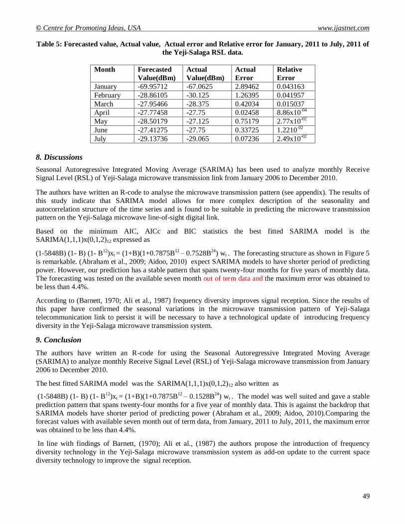
Table 5 below shows the forecast values and observed data for the seven month period from January to July, 2011. The results indicate that the predicted values of SARIMA(1,1,1)x(0,1,2)12 model is close to the true value.

The maximum relative error is less than 4.4 percent. The model is therefore adequate to be used to forecast

monthly RSL data.

Time

data

2006 2007 2008 2009 2010 2011 2012 2013

-70

-60

-50

-40

-30

-20

© Centre for Promoting Ideas, USA www.ijastnet.com

49

Table 5: Forecasted value, Actual value, Actual error and Relative error for January, 2011 to July, 2011 of

the Yeji-Salaga RSL data.

Month Forecasted

Value(dBm)

Actual

Value(dBm)

Actual

Error

Relative

Error

January -69.95712 -67.0625 2.89462 0.043163

February -28.86105 -30.125 1.26395 0.041957

March -27.95466 -28.375 0.42034 0.015037

April -27.77458 -27.75 0.02458 8.86x10-04

May -28.50179 -27.125 0.75179 2.77x10-02

June -27.41275 -27.75 0.33725 1.2210-02

July -29.13736 -29.065 0.07236 2.49x10-02

8. Discussions

Seasonal Autoregressive Integrated Moving Average (SARIMA) has been used to analyze monthly Receive

Signal Level (RSL) of Yeji-Salaga microwave transmission link from January 2006 to December 2010.

The authors have written an R-code to analyse the microwave transmission pattern (see appendix). The results of

this study indicate that SARIMA model allows for more complex description of the seasonality and

autocorrelation structure of the time series and is found to be suitable in predicting the microwave transmission pattern on the Yeji-Salaga microwave line-of-sight digital link.

Based on the minimum AIC, AICc and BIC statistics the best fitted SARIMA model is the SARIMA(1,1,1)x(0,1,2)12 expressed as

(1-5848B) (1- B) (1- B12

)xt = (1+B)(1+0.7875B12

– 0.7528B24

) wt . The forecasting structure as shown in Figure 5

is remarkable. (Abraham et al., 2009; Aidoo, 2010) expect SARIMA models to have shorter period of predicting

power. However, our prediction has a stable pattern that spans twenty-four months for five years of monthly data.

The forecasting was tested on the available seven month out of term data and the maximum error was obtained to be less than 4.4%.

According to (Barnett, 1970; Ali et al., 1987) frequency diversity improves signal reception. Since the results of this paper have confirmed the seasonal variations in the microwave transmission pattern of Yeji-Salaga

telecommunication link to persist it will be necessary to have a technological update of introducing frequency

diversity in the Yeji-Salaga microwave transmission system.

9. Conclusion

The authors have written an R-code for using the Seasonal Autoregressive Integrated Moving Average

(SARIMA) to analyze monthly Receive Signal Level (RSL) of Yeji-Salaga microwave transmission from January

2006 to December 2010.

The best fitted SARIMA model was the SARIMA(1,1,1)x(0,1,2)12 also written as

(1-5848B) (1- B) (1- B12

)xt = (1+B)(1+0.7875B12

– 0.1528B24

) wt . The model was well suited and gave a stable

prediction pattern that spans twenty-four months for a five year of monthly data. This is against the backdrop that

SARIMA models have shorter period of predicting power (Abraham et al., 2009; Aidoo, 2010).Comparing the forecast values with available seven month out of term data, from January, 2011 to July, 2011, the maximum error

was obtained to be less than 4.4%.

In line with findings of Barnett, (1970); Ali et al., (1987) the authors propose the introduction of frequency

diversity technology in the Yeji-Salaga microwave transmission system as add-on update to the current space

diversity technology to improve the signal reception.

International Journal of Applied Science and Technology Vol. 2 No. 9; November 2012

50

References

Abraham, G., Byrnes, G. B. and Bain, C. A. (2009). Short-Term Forecasting of Emergency Inpatient Flow. IEEE

Transactions on Information Technology in Biomedicine, Vol. 13. No. 3. pp. 380-388.

Aidoo, E. (2010). Modelling and Forecasting Inflation Rates in Ghana: An Application of SARIMA Models.

Master’s Thesis. Högskolan Dalarna School of Technology and Business Studies. Sweden. Akter, S. and Rahman, S. (2010). Agribusiness Forecasting with Univariate Time Series Modelling Techniques:

The Case of a Dairy Cooperative in the UK. Journal of Farm Management. Vol. 13. No. 11. pp. 747-764.

Ali, A., Hassan, M. and Alhaider, M. (1987). Experimental Studies of Terrestrial mm-Wave Links- A Review. Part 2: Fading, Diversity and Data Processing. Journal of Engineering Science. Vol. 13. No. 1. pp 139-

153.

Andreeski, C. J. and Vasant, P. M. (2008). Comparative Analysis of Bifurcation Time Series. Biomedical Soft Computing and Human Sciences. Vol.13. No.1. pp. 45-52.

Assis, K., Amran, A. and Remali, Y. (2010). Forecasting Cocoa Bean Prices Using Univariate Time Series

Models. Journal of Arts, Science and Commerce. Vol. 1. No. 1. pp. 71-80.

Barnett, W. T. (1970). Microwave Line-of-Sight With and Without Frequency Diversity. The Bell System Technical Journal. Vol. 49. No. 8. pp 1827-1871.

Box, G. P. and Jenkins, G. M. (1976). Time Series Analysis, Forecasting and Control. Holden-Day. San Francisco. CA.

Brida, J. G. and Risso, W. A. (2011). A SARIMA-ARCH Model for the Overnight-Stays Tourism in South Tyrol. Tourism Economics. Vol. 17. No. 1. pp. 209–222.

Chandra, S. R. and AI-Deek, H. M. (2009). Predictions of Freeway Traffic Speeds and Volumes Using Vector

Autoregressive Models. Journal of Intelligent Transportation Systems. Vol. 12. No. 2. pp. 53-72.

Chen, H. and Trajkovi´c, L. (2004). Prediction of Traffic in a Public Safety Network. School of Computing Science, Simon Fraser University. Burnaby. Canada. www.ensc.sfu.ca/~ljilja/papers/iswcs2004.pdf

Chen, S. M. (1996). Forecasting Enrollments Based on Fuzzy Time Series. Fuzzy Sets and Systems. Vol. 81. No.

3. pp. 311–319. Engle, R. F. (2001). GARCH 101: The Use of ARCH/GARCH Models in Applied Econometrics. Journal of

Economic Perspectives. Vol. 15. No. 4. pp. 157-168.

Glosten, L., Jagannathan, R. and Runkle, D. (1993). On the Relation Between Expected Value and the Volatility of the Nominal Excess Return on Stocks. Journal of Finance. Vol. 48. pp. 1779-1801.

Huang, G. (1997). Signal Fading on Microwave Links. Master’s Thesis. Faculty of Engineering Science.

Department of Electrical and Computer Engineering. University of Western Ontario. Ontario. Canada.

Javedani, H., Lee, M. H. and Suhartono, (2010). An Evaluation of some Classical Methods for Forecasting Electricity Usage on Specific Problem. Journal of Statistical Modeling and Analytics. Vol. 2. No. 1. pp. 1-10.

Kahforoushun, E., Zarif, M. and Mashahir, E. R. (2010). Prediction of added value of Agricultural

Subsections Using Artificial Neural Networks: Box-Jenkins and Holt-Winters Methods. Journal of

Development and Agricultural Economics. Vol. 2. No. 4. pp. 115-121. Li, X. (2009). Applying GLM Model and ARIMA Model to the Analysis of Monthly Temperature of Stockholm.

D-level Essay in Statistics. Department of Economics and Society. Dalarna University. Sweden.

Loganathan, I., Nanthakumar, I. and Ibrahim, Y. (2010). Forecasting International Tourism Demand in Malaysia Using Box Jenkins SARIMA Application. South Asian Journal of Tourism and Heritage. Vol.

3. No. 2. pp. 50-60.

Nobre, F. F., Monteiro, A. B. S.; Telles, P. R. and Williamson, D. (2001), Dynamic Linear Model and

SARIMA: A Comparison of their Forecasting Performance in Epidemiology, Statistics in Medicine. Vol. 20. No. 20. pp. 3051-3069.

Permanasari, A. E., Rambli, D. R. A. and Dominic, P. D. D. (2009). Prediction of Zoonosis Incidence in

Human using Seasonal Auto Regressive Integrated Moving Average (SARIMA). International Journal of Computer Science and Information Security. Vol. 5. No. 1. pp. 103-110.

Salema, C. (2003). Microwave Radio Links: From Theory to Design. John Wiley and Sons. New Jersey.

Saz, S. (2011). The Efficacy of SARIMA Models for Forecasting Inflation Rates in Developing Countries: The Case for Turkey. International Research Journal of Finance and Economics. Vol. 62. pp. 112-142.

Schuster, A. (1906). On the Periodicities of Sunspots. Philosophical Transactions of the Royal Society:

Proceedings of the Royal Society of London. Series A. Containing Papers of a Mathematical and Physical

Character. Vol. 77. No. 515. pp. 141-145.

© Centre for Promoting Ideas, USA www.ijastnet.com

51

Shekhar, S. (2004). Recursive Methods for Forecasting Short-Term Traffic Flow using Seasonal ARIMA Time

Series model. Master’s thesis. Graduate Faculty of North Carolina State University. Raleigh. North

Carolina. USA.

Sims, C. (1977). Macroeconomics and Reality. Econometrica. Vol. 48. No. 1. pp.1-48. Song, Q. and Chissom, B. S. (1993). Fuzzy Time Series and its Models. Fuzzy Sets and Systems. Vol. 54. No.3.

pp. 269–277.

Tanaka, H. (1987). Fuzzy Data Analysis by Possibility Linear Models. Fuzzy Sets and Systems. Vol. 24. No. 3. pp. 363-375.

Tanaka, H. and Ishibuchi, H. (1992). Possibility Regression Analysis Based on Linear Programming in Fuzzy

Regression Analysis. J. Kacprzykx and M. Fedrizzi, eds., Omnitech Press. Warsaw and Physica-Verlag. Heidelberg. pp. 47–60.

Tanaka, H., Uejima, S. and Asai, K. (1982). Linear Regression Analysis with Fuzzy Model. IEEE Transactions

on Systems, Man and Cybernetics. Vol. 12. No. 6. pp. 903–907.

Tsay, R. S. (2010). Analysis of Financial Time Series. Third Edition. John Wiley and Sons Inc., Hoboken, New Jersey, USA.

Tseng, F. M. and Tseng, G. H. (2002). A Fuzzy Seasonal ARIMA Model for Forecasting. Fuzzy Sets and

Systems. Vol. 126. pp 367-376. Tseng F.M.; Tzeng, G.H.; Yu, H.C. and Yuan, B. J. C. (2000). Fuzzy ARIMA Model for Forecasting the

Foreign Exchange Market. Fuzzy Sets and Systems. Vol. 118. pp. 9 –19.

Wongkoon, S., Pollar. M., Jaroensutasinee, M. and Jaroensutasinee. K. (2008). Predicting DHF Incidence in Northern Thailand using Time Series Analysis Technique. International Journal of Biological and Life

Sciences. Vol. 4. No.3. pp. 117-121.

Xiang, J. (2008). Applying ARIMA Model to the Analysis of Monthly Temperature of Stockholm. Master’s

thesis in Statistics. Department of Economics and Society. Dalarna University. Sweden. Yan, W., Xu, Y., Yang, W and Zhou, Y. (2010). A Hybrid for Short-Term Bacillary Dysentery Prediction in

Yichang City, China. Japanese Journal of Infectious Disease. Vol. 63. pp. 264-270.

Yantai, S., Minfang. Y., Oliver, Y., Jiankun, L. and Huifang, F. (2005). Wireless traffic modeling and Prediction using seasonal ARIMA models. The Institute of Electronics, Information and Communication

Engineers (IEICE) Transaction on Communications. Vol. 88. No. 10. pp. 3992-3999.

Yule, G. U. (1927). On a Method of Investigating Periodicities in Disturbed Series with Special Reference to

Wolfer’s Sunspot Numbers. Philosophical Transactions of the Royal Society. Vol. 226. pp. 1-422.

Appendix

R-CODE FOR SARIMA TIME SERIES MODEL

data = read.table (“C:\\Documents and Settings\\Administrator\\Desktop\\data.txt”, header = TRUE)

data= ts (data, start= (2006),frequency=12) plot(data,main =”Time Series Plot of Receive Signal Level”, xlab="Time(year)", ylab="Receive Signal

Level(dBm)")

datadiff = diff(data, 12)

plot(datadiff, main="Series:datadiff", xlab="Time(year)",ylab="Receive Signal Level(dBm)") load(“C:\\Users\\USER\\My Documents\\tsa3.rda”)

acf2(datadiff,46)

sarima(data,1,1,1,0,1,2,12) sarima(data,1,1,1,1,1,2,12)

sarima(data,1,1,1,1,1,1,12)

sarima(data,1,1,1,1,1,0,12) sarima.for(data,24,1,1,1,0,1,2,12)

history()