“Steady State and Dynamic Simulation of Cryogenic system

for Superconducting Linear Accelerator (LINAC) at TIFR”

SANTOSH S. JANGAM

Tata Institute of Fundamental Research, Mumbai, INDIA

Indian Institute of Technology, Kharagpur, INDIA

Fermilab, Batavia, IL 1st June 2011

The Outline of the Presentation

Introduction of Superconducting LINAC and its

Cryogenic system

Steady State Simulation of Linde TCF-50S

refrigerator plant using ASPEN HYSYS

Characterization of the Expander, Heat exchanger,

Valve & Dewar

Dynamic Simulation of Linde TCF-50S using Hysys

Pressure Drop and Heat load calculation of

Cryogenic Distribution system.

Upgradation of TCF 50S at TIFR

Conclusion

Introduction

Particle Accelerator is essential tool in Nuclear Physics,

Condensed matter physics, Radiation Physics, Material science,

Bio-Physics, Bio-medical and Energy generation.

High accelerated beam of Heavy ions is possible with

Superconducting LINAC.

Why superconducting ?

Q=f/Δf=ωU/P ; Quality factor

P ~ ½ R ∫I2 ds and U = ∫E2 dv ~ ½ C V2 or ½ L ∫I2 ds, hence Q=L / R

LINAC QWR: f=150MHz, ω~109

E~3 MV/m, U (stored energy) ~0.5 Joules

Q(Cu, 300K)~104; P~50 kWatts, Q(Pb, 4.2K) ~108; P~5 Watts

The LINAC QWR are operated at liquid helium temperature (~4.2 K)

Superconducting LINAC smaller & efficient

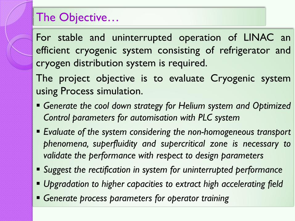
For stable and uninterrupted operation of LINAC an

efficient cryogenic system consisting of refrigerator and

cryogen distribution system is required.

The project objective is to evaluate Cryogenic system

using Process simulation.

Generate the cool down strategy for Helium system and Optimized

Control parameters for automisation with PLC system

Evaluate of the system considering the non-homogeneous transport

phenomena, superfluidity and supercritical zone is necessary to

validate the performance with respect to design parameters

Suggest the rectification in system for uninterrupted performance

Upgradation to higher capacities to extract high accelerating field

Generate process parameters for operator training

The Objective…

The Superconducting Linear Accelerator has been indigenously developed to

boost the energy of heavy ion beams delivered by the Pelletron accelerator.

Development of the superconducting LINAC is a major milestone in the

accelerator technology in INDIA. It was commissioned in JULY 2007.

Introduction of LINAC

SpecificationsHeavy ions upto A~80

E / Z~5-12 MeV

Energy gain 14MV/q

Acceptance ~b= 0.1

Module 7 nos

Resonators 28 nos

Bunch width ~200 ps

Beam Intensity 0.1-10 pnA

View of LINAC

View of LINAC Cryostats and its associated RF and Cryogenic System

New user beam hall and experimental area

Qs: Most probable charge state at terminal foil stripper

Epell (bpell): Energy (velocity) at Pelletron exit

Qs2: Most probable charge state after post tandem foil stripper

Z A Qs b Epell(MeV) Qs2 Elinac (MeV)

O 8 16 6 0.106 84 8 150

F 9 19 6 0.097 84 8 150

Si 14 28 8 0.091 108 12 210

S 16 32 8 0.085 108 14 230

Cl 17 35 9 0.086 120 15 250

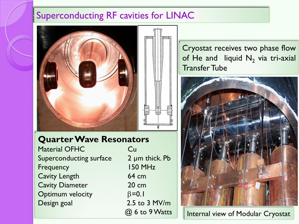
Superconducting RF cavities for LINAC

Internal view of Modular Cryostat

Cryostat receives two phase flow

of He and liquid N2 via tri-axial

TransferTube

Quarter Wave ResonatorsMaterial OFHC Cu

Superconducting surface 2 µm thick. Pb

Frequency 150 MHz

Cavity Length 64 cm

Cavity Diameter 20 cm

Optimum velocity b=0.1

Design goal 2.5 to 3 MV/m

@ 6 to 9 Watts

Schematic of Cryogenic system for LINAC

Custom-built liquid helium refrigerator TCF 50-S

Linde Kryotechnik

The Distribution system consists of

Main Junction box

Distribution Trunk lines

Remote filling stations

TransferTubes

Loop-back end box

A 300 litres Dewar is used as a source of the liquid

Nitrogen supplied by Low Temp. Facility of TIFR.

Helium Refrigerator LINDE TCF- 50s

Based on modified Claude cycle.

Refrigeration, Liquefaction capacity

Old Configuration: Without LN2 300W @ 4.5 K, 50 l/hr

Upgraded Configuration:Without LN2 410W @ 4.5 K, 75 l/hr

The two-phase helium at 4.5 K produced at the JT stage in the refrigerator

is delivered to the cryostats through a Cryogen Distribution system.

View of Helium Refrigerator LINDE TCF- 50s and LN2 storage

Cryogen distribution system for LINAC

• Vacuum insulated trunk line,

100mm in diameter has four tubes

• Made in separate sections with

Kenol fittings supported by Teflon

spacer

Individual triaxial transfer tubes of the cryostat serve as a final heat

exchanger and a remote JT

Transfer Tube

Trunk Line

Part 1: Refrigerator Process simulation

Steady state simulation

For rating and design of the refrigerator.

The upgradation of refrigerator to higher capacity

Generate process parameters for operator training

Parametric study of major components such as Turbine,

Heat Exchanger,Valve and Dewar

Loss in refrigeration capacity due to off-design operation

Dynamic simulation

Cool-down behavior of the plant in refrigeration mode

Operation of the plant at elevated discharge pressure.

Heat load fluctuations, pulsed load and disturbances to

plant.

Control parameter values for the PLC‟s

Part 11: Evaluation of Cryogenic distribution system

Evaluation of the cryogenic system considering the non-

homogeneous transport properties and Heat inleak.

A. The frictional pressure drop calculation:

To estimate the loss in the refrigeration capacity.

Calculation of the control parameters like Pressure,

and Valve opening to achieve equal flow in each

cryostats.

B. Calculation of the standalone heat load on system.

The loss in refrigeration due to conduction and

radiation heat transfer.

General purpose modular-sequential process simulator

Easy Process Flow-sheet Generation with inbuilt blocks for

Compressor, Expander, Heat Exchanger (LNG), Phase

Separator

Aspen Muse® software makes it possible to simulate

complex plate-fin heat exchangers

Easy to Switch from Steady State to Dynamics

Dynamic Assistant

Availability of Advanced Control Algorithms

Logical Operations and Spread Sheet

Easy Customization of Components

Accuracy of Helium Property Data up to 2.2 K

Commercial simulator Aspen HYSYS®

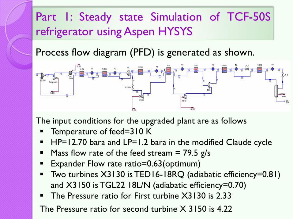
Part 1: Steady state Simulation of TCF-50S

refrigerator using Aspen HYSYS

Process flow diagram (PFD) is generated as shown.

The input conditions for the upgraded plant are as follows

Temperature of feed=310 K

HP=12.70 bara and LP=1.2 bara in the modified Claude cycle

Mass flow rate of the feed stream = 79.5 g/s

Expander Flow rate ratio=0.63(optimum)

Two turbines X3130 is TED16-18RQ (adiabatic efficiency=0.81)

and X3150 is TGL22 18L/N (adiabatic efficiency=0.70)

The Pressure ratio for First turbine X3130 is 2.33

The Pressure ratio for second turbine X 3150 is 4.22

Loss in refrigeration capacity due to off-design operation;;

Using Aspen Hysys® the refrigeration capacity is calculated for different

J-T outlet pressure

The mass energy balance across Dewar

The loss is around ~16 W in steady state for operating at 1.5 bara for 29 g/s

and about 10 W for 20 g/s .

12 11( )( )a eQ m m h h=

29 20em m g sand g s =

Loss in refrigeration capacity with variation in after J-T pressure

P (bar a)

1.1 1.2 1.3 1.4 1.5 1.6 1.7 1.8 1.9

Qa (

Watt

s)

250

300

350

400

450

500

29 g/s

20 g/s

Characterization study of components: Turbine

Turbine pressure ratio (pr)

1.6 1.8 2.0 2.2 2.4 2.6 2.8 3.0 3.2 3.4 3.6

0.050

0.051

0.052

0.053

0.054

0.055

0.056

0.057

4800 rps

4600 rps

4400 rps

4200 rps

4000 rps

3800 rps

3600 rps

no

n d

ime

ns

ion

al

mas

s f

low

rate

(

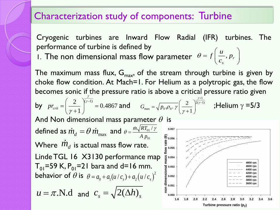
Cryogenic turbines are Inward Flow Radial (IFR) turbines. The

performance of turbine is defined by

1. The non dimensional mass flow parameter , r

s

uf p

c

=

The maximum mass flux, Gmax, of the stream through turbine is given by

choke flow condition. At Mach=1. For Helium as a polytropic gas, the flow

becomes sonic if the pressure ratio is above a critical pressure ratio given

by and ;Helium g =5/3

And Non dimensional mass parameter is

defined as and

Where is actual mass flow rate.

LindeTGL 16 X3130 performance map

T01=59 K, P01=21 bara and d=16 mm.

behavior of is

and

1

2( 1)

max 0 0

2. .

1G p

g

g

gg

=

( 1)2

10.4867critpr

g

g

g

=

=

max dm m=

dm

01

01

/

m RT

A p

g =

2

0 1 2( / ) /s sa a u c a u c =

.N.du = 2( )s sc h=

Continue…

2. Radial turbine efficiency

Turbine stages exhaust in a closed space hence the kinetic energy is of

the outgoing jet is lost because it is not used after the turbine Therefore

total to static efficiency is

Turbine characteristics curve for small capacity expander ( < 0.055) are

retrieved from empirical performance curves.

,T r

s

uf p

c

=

01 02 01 02

01 2 01 2

( )

( )s

s s

h h T T

h h T T

= =

Turbine pressure ratio (Pr)

1.6 1.8 2.0 2.2 2.4 2.6 2.8 3.0 3.2 3.4

Tu

rbin

e t

ota

l to

sta

tic e

ffic

ien

cy (

%)

40

45

50

55

60

65

70

75

80

4600 rps

4400 rps

4200 rps

4000 rps

3800 rps

3600 rps

The Linde TGL 16 X3130

N=4600 rps, d=16 mm,

The entrance velocity ratio

u/cs= 0.625; optimal is 0.7

Mach number M=0.863

From performance curves

@ Pr=2.4 ; s=76%, = 0.055

Hence

max maxm =G .A=884g s

max 47.5 / dm m g s ==

Heat Exchanger

The rating of Heat exchanger determines the following performance parameters of

Heat Exchanger.

Overall Heat Transfer Coefficient: UA

The Colburn factor jh ;

The total heat transfer is ; Tlm is LMTD

Density, viscosity, specific heat, etc., in the duct were variable, and calculated using

HEPAK® at mean fluid temperature. The fin material was assigned a variable

thermal conductivity and specific heat. Aspen MUSE was used to simulate the

existing HEAT exchanger.The data is

Main Fins Geometry:

Height 8.90 mm, Frequency 787 fins/m, thickness 0.203 mm Fin type: serrated fins

, ,

0 0 0 0

1 1 1

( ) ( ) ( ) ( )

f c f h

w

c c h h

RUA hA A

R R

A hA =

2/3PrcH

p ff

hJ

c m A=

lmq UA T=

Heat exchanger 3110A 3120A 3120B3140, Three

stream3150 3160A 3160B

Mass flow rate Hot 79 g/s 79 g/s 29 g/s 29 g/s 50 g/s 29 g/s 29 g/s 29 g/s

Mass flow rate cold 79 g/s 79 g/s 79 g/s 79 g/s 79 g/s 29 g/s 29 g/s

HX dimension

(LxHxW) (mm) 966x504x449 1136x306x271 364x118x122 1061x365x318 1228x148x133 1140x207x183 798x128x132

Total surface area (m2) 211.03 107.55 4.54 123.10 26.80 49.44 13.99

UA (kW/K) 12.252 9.339 0.753 2.39 3.058 2.63 1.218

Heat Duty (kW) 65 46.5 1.5 7.9 1.0 0.7 0.3

Heat Exchanger continue…

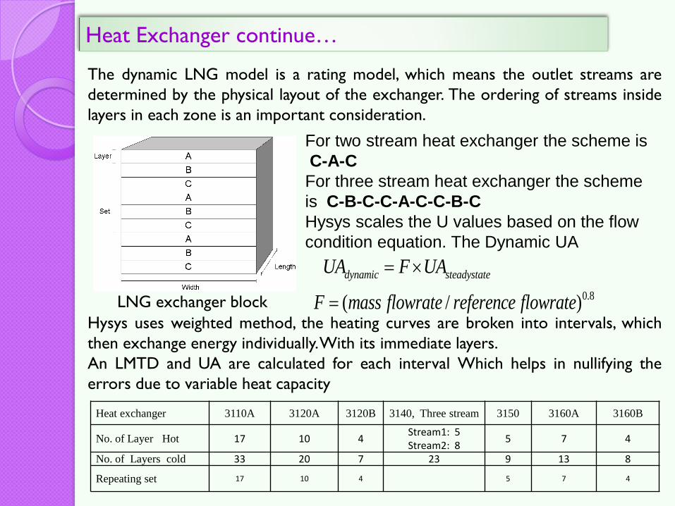
The dynamic LNG model is a rating model, which means the outlet streams are

determined by the physical layout of the exchanger. The ordering of streams inside

layers in each zone is an important consideration.

Hysys uses weighted method, the heating curves are broken into intervals, which

then exchange energy individually.With its immediate layers.

An LMTD and UA are calculated for each interval Which helps in nullifying the

errors due to variable heat capacity

For two stream heat exchanger the scheme is

C-A-C

For three stream heat exchanger the scheme

is C-B-C-C-A-C-C-B-C

Hysys scales the U values based on the flow

condition equation. The Dynamic UA

dynamic steadystateF UAUA =

0.8( / )F mass flowrate reference flowrate=LNG exchanger block

Heat exchanger 3110A 3120A 3120B 3140, Three stream 3150 3160A 3160B

No. of Layer Hot 17 10 4Stream1: 5Stream2: 8

5 7 4

No. of Layers cold 33 20 7 23 9 13 8

Repeating set 17 10 4 5 7 4

Valve

Types of plugs and valve seats which are changed in upgraded plant

;;

The general valve equation

Linear:

Quick Opening:

Equal Percentage:

( ) /vq C f z p G=

( )f z Z=

( )f z z=1( ) ,zf z R R is rangeable=

Where k value is specified to get the desired pressure and Flowrate.

Care needs to take that the flow should not be choked.

Auto sizing in Hysys helps to size the valve.

In our calculation we are using the Simple

Resistance Equation to size the valve

m density valveopening p=

Hysys allows to select type of valve depend upon the requirements

Dewar

Aspen Hysys® Phase separator module can

be used to accurately model and simulate a

Helium Dewar in a process environment.

The vessel is equipped with a Helium level sensor and electrical heater(230V/600 W)

Heater is used to balance the cold box. The refrigeration capacity is measured using

this heater.

. . . .

2.41 3.20 0.277 5.887 ~ 6total rad cond g

Q Q Q Q W W W W W= = =

Part 1I: Dynamic Simulation of TCF-50S refrigerator

The cool down of Dewar and the refrigeration capacity of the plant in dynamics is

simulated. Following Assumption are made

The mass flow to the plant is constant and at constant pressure since buffer is

used in plant. Compressor unit is not included in simulation

The turbine adiabatic efficiency and outlet pressure is fixed. This can be done

rigorously by using characteristic curves and speed of the turbine.

The standing heat load of Dewar is considered as ~6 W.

For refrigeration calculations built-in heater (i.e. direct Q) to Dewar is used.

pipes connecting all the components are not considered for any hold up

calculations

The PFD is generated as follows:

Continue…

The simulation is performed on the Intel® core® 2 Quad CPU at

2.66 GHz with 4 GB of RAM.

Simulated cool down time was 10 hrs. Observed cool down for Dewar is

around 12 hrs.

The time taken for simulation was 30 minutes of computation time. The

real time factor was 10.0 times and with acceleration of 2.0. Hence

Simulator ran 20 times faster than the real process.

The integration step size used is 0.5 seconds.

The total equation summary of model is

Number of equations 276

Number of variables 276

User Spec Equations 9

User Spec Variables 9

Internal Spec Equation 3

Internal spec variables 3

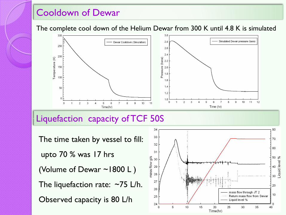
Cooldown of Dewar

The complete cool down of the Helium Dewar from 300 K until 4.8 K is simulated

The time taken by vessel to fill:

upto 70 % was 17 hrs

(Volume of Dewar ~1800 L )

The liquefaction rate: ~75 L/h.

Observed capacity is 80 L/h

Liquefaction capacity of TCF 50S

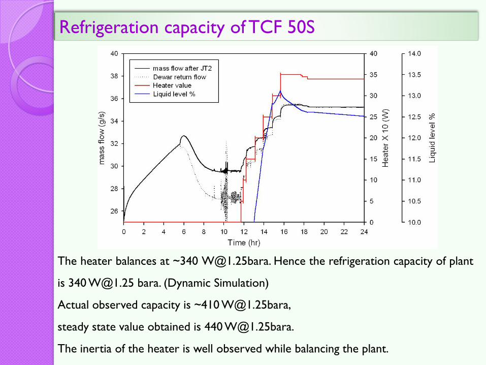
Refrigeration capacity of TCF 50S

The heater balances at ~340 W@1.25bara. Hence the refrigeration capacity of plant

is 340 W@1.25 bara. (Dynamic Simulation)

Actual observed capacity is ~410 W@1.25bara,

steady state value obtained is 440 W@1.25bara.

The inertia of the heater is well observed while balancing the plant.

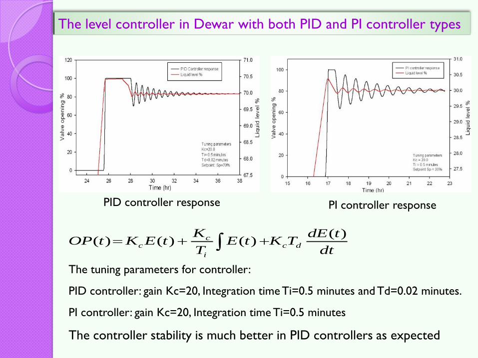
The level controller in Dewar with both PID and PI controller types

The tuning parameters for controller:

PID controller: gain Kc=20, Integration time Ti=0.5 minutes and Td=0.02 minutes.

PI controller: gain Kc=20, Integration time Ti=0.5 minutes

The controller stability is much better in PID controllers as expected

PID controller response PI controller response

( )( ) ( ) ( )c

c c d

i

K dE tOP t K E t E t K T

T dt=

Pressure Drop calculation:

Pressure in mbar

P0 P1 P2 P3 P4 P5 P6 P7

1361.4 1365.1 1365.4 1365.4 1367.2 1367.2 1367.8 1367.8

Valve mass attenuation factor

V0 V1 V2 V3 V4 V5 V6 V7

0.04 0.10 0.10 0.10 0.22 0.22 1.00 1.00

For equal flow in all module cryostats, the valve openings vary over a wide range

(0.1 to 1.0). This can be attributed to the asymmetry of distribution between the

two parts of the LINAC. Very small pressures changes (~10 mbar) in the supply lines,

significantly affect the valve openings.

Pressure drop per unit length is

G is the mass flux

Helium is in better agreement with the homogeneous model hence to

predict the two phase flow this model was used over the separated flow

model of Lockhart and Martinelli (1949)mean density is related to fluid quality “x” by

The viscosity used in the Reynolds number is a

mean viscosity, defined by McAdams (1942)

The simultaneous equation obtained are solved, the following output was obtained

for

2

2

P fG

l D

=

1 (1 )

m L G

x x

=

1 (1 )

m L G

x x

=

7 1.0V =

1.2RP bara=

s 1.51P bara=

Continue…

The pressure drop across the valve as a function

of valve opening in terms of mass attenuation

factor „v’ is

Pressure drop versus mass attenuation factor

For

1

1.8vm vC P=

29 /m g s=

Output of the Homogeneous flow model with varying quality factor

;;

The frictional losses in the distribution line are very high if the quality factor x

of two phase produced after second Joule Thomson is high. Hence TCF50S has double JT

system so we can always get low quality factor.

The homogeneous flow model reproduces fairly well, the observed values during the actual

operation of the LINAC

Heat load calculation:

Estimated Heat Load (W) Heat Load (W) Heat Load (W)

Phase I Phase II Old Plant Upgraded

The mass flow from compressor 62 g/s 79 g/s

The mass flow through distribution system 20 g/s 29 g/s

The deviation of operating point from the

rated value---- ---- 10W 16 W

Frictional drag losses ---- ---- 32W 55 W

Heat Load in He Dewar 6 W 6 W 6 W

Distribution box, main box and trunk line 16 W 16 W 32W 32 W

Transfer tube and cryostat, 12W each 4X12W=48W 4X12W=48W 96W 96 W

QWR @6W each and Superbuncher @4W12x6W=72W

1 x 4W =4W16x6W=96W 172W 172 W

Total (Phase I + II) 306 W 348W 377 W

In our system there are two major causes of heat load:

Conduction due to supports and radiation from surroundings at higher temperatures.

Due to the flow, there is a continuous frictional drag which results in heat dissipation. And

given by

Calculating the upper limit of the heat load by assuming the supply pressure 1.6 bara and

return pressure 1.2 bara, we get available refrigeration capacity

Summary of total standalone Heat Load in Cryogenic System

R S

dQ; m H H

dt= S R

R S S R

dV dVdQm U U P P

dt dt dt

=

; Supply point is S return point is R

Upgradation of TCF50S plant

The upgradation of TCF50S was carried out at TIFR site in December 2010.

The compressor which delivers 80g/s was installed Associated ORS system was

replaced. The valve seats of the control valves are changed to accommodate the

higher mass flow rates. Due to a higher mass flow first expansion turbine X3130 in

the cold box was replaced with a larger unit.

Turbine TED 16

internal view of TCF 50S

Conclusions

The Available refrigeration capacity is 410W hence with the heat load of

377W LINAC operations is possible without the Nitrogen Precooling. The

measured refrigeration capacity using built-in heater in DEWAR is ~410 W.

We still left with 33 W which could be utilized to run the RF cavities at

higher dissipating power of ~7 W each. This helps to get higher accelerating

field in the resonators and ultimately the higher energy gain.

The Dynamic Simulations was done with the coldbox as

liquefier/refrigerator mode. The real data will be obtained shortly for

comparison. The coldbox is still conditioning and different parameters for

controllers and valve settings needed tuning. The data from Dynamic

simulation is helpful for generating control strategies and optimizing the

system.

Conclusions

The characteristic curves for turbines must be considered when

refrigerator simulation is modeled. This will accurately calculate the

efficiency and head with varying speeds of turbine and hence producing

better simulation results.

The controller settings and performance was simulated. The PID controllers

are much stable feedback controllers than PI or P-only controllers.

We upgraded the existing plant with higher mass flow rate (~79 g/s).The

existing TCF 50S refrigeration plant is modified to get the higher

refrigeration capacity. The new turbine and the control valve seats are

changed to accommodate the higher mass flow rate. After upgradation the

new calculated capacities are; without LN2: Refrigeration: 410 W at 4.5 K,

Liquefaction: 80 l/hr.

THANK YOU