santosh mohan rajkumar (13-1-3-015) sayan chakraborty (13
TRANSCRIPT
Development of Embedded Speed Control System for DC
Servo Motor using Wireless Communication
By Santosh Mohan Rajkumar (13-1-3-015)
Sayan Chakraborty (13–1-3-007)
A thesis submitted in partial fulfillment for the
degree of Bachelor of Technology in Electrical Engineering
Under The Guidance of
Dr. Rajeeb Dey
Department of Electrical Engineering
National Institute of Technology, Silchar
December 2019


Declaration
We, Santosh Mohan Rajkumar (13-1-3-015), and Sayan Chakraborty (13-1-3-007)
declare that this thesis titled, ”Development of Embedded Speed Control System
for DC Servo Motor using Wireless Communication” and the work presented in
it are our own. We confirm that:
□ This work was done wholly or mainly while in candidature for B.Tech. degree at
National Institute of Technology, Silchar.
□ Any part of this thesis has not previously been submitted for a degree or any
other qualification at this institute or any other institutes.
□ Where we have consulted the published work of others, this is always clearly
attributed.
□ Where we have quoted from the work of others, the source is always given. With
the exception of such quotations, this thesis is entirely our own work.
□ We have acknowledged all main sources of help.
Signature:
Date:
iii

“Peace comes from within, don’t seek it without”
The Tathagata

Abstract
With the advancement of computer technology and digital systems, wireless control
systems or Wireless Networked Control Systems(NCS) are becoming increasingly pop-
ular among the scientific community as well as the industry due to their flexibility,
convenience & ease of operation. In this experiment, a closed-loop discrete time sys-
tem for speed control of a permanent magnet DC motor with discrete PI controller is
implemented in embedded platform. The design & analysis of the system is based on
the mathematical model of the DC motor obtained by system identification technique.
After that the closed loop system is distributed through a wireless network created
by means of Bluetooth without any change in the discrete controller. The network
connects the controller on one side with the sensor, actuator & the plant on the other
side. Then the performance of the closed loop system is observed with the wireless
network in two configurations : with point-to-point connection between two nodes and
a network structure with two intermediate nodes among the controller side node & the
plant side node. It has been observed that the performance degrades with only the PI
controller a little bit in point to point configuration and the performance severely de-
grades in intermediate node configuration. To tackle this issue time delay is measured
in the WNCS and then a digital smith predictor structure is implemented to obtain
better performance. It has been observed that in point to point configuration the time
delay remains almost constant and in intermediate node configuration the time delay is
varying. Hence the digital smith predictor fails to perform reasonably in intermediate
node configuration. An online time delay measurement & estimation procedure has
been implemented and proposed in this research. We have implemented an adaptive
digital smith predictor using the online time delay measurement and identification.
The implemented smith predictor provides good results for both intermediate node
and point to point connection. An stability analysis of the DC motor system with
variation of delay has been discussed.

Acknowledgements First and foremost, we feel it as a great privilege in expressing our deepest and most
sincere gratitude to our supervisor Dr. Rajeeb Dey, for providing us an opportunity
to work under him and for his excellent guidance. His kindness, friendly accessibility
and attention to details have been a great inspiration to us. Our heartiest thanks to the
supervisor for the support, motivation and the patience he has shown to us. His
suggestions and advice have been always constructive. We hope that we will be able
to pass on the research values and knowledge that he has given given to us.
We are also very much thankful to Mr. Nalini Prasad Mohanty and Mr. Anirudh Nath
(PhD scholars) for their support, guidance and help. Their friendly behaviour and kind
cooperation made the environment productive.
We are also grateful to Prof. Binoy Krishna Roy for his instrumental suggestions
for continuous improvement in research. He is the back bone of the Control System
Research Community of NIT Silchar. We are proud to have such an experienced and
wise professor in our department.
We would not have contemplated this road without our parents who support us, care
for us and give motivations.
We would also like to express our heartiest gratitute to Mr. Prasanta Roy who taught
us the foundations of Control Engineering. He is a great teacher.
All the faculty members and scholars of the EE department of NIT Silchar, helped us
in many ways to accomplish this project.. . .
vi

Contents
Declarationiii
Abstractv
Acknowledgementsvi
List of Figuresxi
List of Tablesxv
1 Introduction1
1.1 Motivations ................................................................................................ 5
1.2 Problem Statement ................................................................................... 6
1.3 Literature Review ....................................................................................... 6
1.4 Thesis Outline ............................................................................................ 9
1.5 Chapter Summary ....................................................................................10
References10
2 Plant Modeling, Controller Design and The Practical DC Motor Speed
Control System13
2.1 Armature Voltage Control For Speed Regulation .................................... 14
2.1.1 Chopper Control of Separately Excited dc Motors ..................... 14
2.2 Hardware Components Used ................................................................... 15
2.2.1 Arduino Micro Controller Board .................................................. 15
2.2.1.1 Ardunio UNO .................................................................. 16
2.2.1.2 Arduino Due .................................................................. 17
2.2.2 The Bluetooth module .................................................................. 18
2.2.3 The Motor Driver IC .................................................................... 18
2.2.4 The Optical Speed Encoder ........................................................ 19
2.3 Speed Measurement by Optical Encoder ............................................... 19
2.3.1 Optocoupler .................................................................................... 20
2.3.2 Speed Encoder Disc ........................................................................ 21
vii

2.3.3 Calculations for Speed Measurement ......................................... 21
2.4 System Identification ................................................................................ 22
2.4.1 Purpose of System Identification................................................... 22
2.4.2 Different Approaches For System Identification ........................... 22
2.4.3 Systematic Procedure for Identification ....................................... 23
2.4.4 The Toolbox Used For System Identification ..............................24
2.4.5 The Data Samples Used For Model Identification .....................25
2.4.6 Linear Least-Squared Error Minimization for System Identification26
2.4.7 Nonlinear Least-Squared Error Minimization for System Identi-
fication ............................................................................................ 28
2.4.8 Mathematical Approach to Modeling of DC Motor .................. 30
2.4.9 Result of System Identification of the DC Motor ....................... 31
2.4.10 Selection of Model Representing the Actual System ................. 31
2.5 Sampling Time Decision For Discretization of the Plant ........................ 33
2.6 Discretization of the Closed Loop System ............................................... 34
2.6.1 The Closed Loop Pulse Transfer Function ................................... 34
2.6.2 Pulse Transfer Function of Dicrete PI Controller ........................ 37
2.6.3 Tuning of the Discrete PI Controller ......................................... 39
2.6.3.1 Tuning Discrete PI Controller in MATLAB PID Tuner39
2.6.3.2 Root Locus Design of Discrete PI Controller ............... 41
2.7 Practical Implementation of Discrete PI Controller on µC ...................... 42
2.8 Chapter Summary ................................................................................... 46
References46
3 Bluetooth Technology & The Wireless Networked Control System47
3.1 Introduction ............................................................................................... 47
3.2 General Communication Network Architecture ....................................... 48
3.3 The Bluetooth Radio ................................................................................ 50
3.4 Bluetooth as WPAN ....................................................................................... 51
3.4.1 General Requirements of a WPAN ................................................ 51
3.4.2 Difference of WPAN from WLAN ................................................ 51
3.5 The Bluetooth Protocol Stack ................................................................. 52
3.5.1 Security in Bluetooth Protocol ...................................................... 54
3.6 Bluetooth Communication Topology ..................................................... 55
3.6.1 Bluetooth Piconet WPAN ................................................................ 55
3.6.2 Bluetooth Scatternet WPAN ........................................................ 56
3.7 States of a Bluetooth Device .................................................................... 57
3.8 Different Versions of Bluetooth .............................................................. 57
3.9 HC-05 Bluetooth Module .......................................................................... 60
3.9.1 Connection of HC-05 with Arduino Board .................................60
Contents ix
3.9.1.1 Baud Rate .................................................................... 61
3.9.1.2 Software Serial Transmitter and Receiver in Arduino
Board ............................................................................. 62
3.9.2 Configuration of HC-05 Using AT Commands .......................... 62
3.9.3 Bluetooth Connection Between Two Arduino Boards ............... 65
3.10 The Practical Wireless Networked Control System ................................. 66
3.10.1 Testing of the Wireless Network To Used in Control Loop. . .68
3.11 Practical Wave-forms of the wireless Setup with PI Controller ............ 69
3.11.1 WNCS With Software Defined Serial Port ................................ 71
3.12 Chapter Summary ................................................................................... 72
References72
4 Time Delay Measurement, Estimation, Aprroximation & Smith Pre-
dictor Scheme for Delay Compensation73
4.1 Time Delay in Network Control System .................................................. 73
4.2 Time Delay Measurement and Estimation in Wireless Network Control
System........................................................................................................ 75
4.3 Practical Implementation of The Proposed RTT Measurement in [1]
With Necessary Modifications ................................................................. 77
4.4 Time-Delay Approximation .................................................................... 82
4.5 Implementation of the Approximated Time-Delay ................................. 84
4.6 Introduction to Smith Predictor .............................................................. 87
4.7 The Smith Predictor Scheme .................................................................... 87
4.7.1 Adaptive Smith Predictor ........................................................... 89
4.7.2 Digital Smith Predictor ................................................................. 90
4.8 Implementation of Digital Smith Predictor in WNCS .......................... 91
4.8.1 Digital Smith Predictor With Intermediate Communication Nodes93
4.8.2 Adaptive Digital Smith Predictor ................................................ 96
4.8.3 Implementation of Discrete Transfer Function in Embedded Plat-
form ............................................................................................... 99
4.9 Practical Waveforms Obtained from Extensive Experimentation of the
Digital Smith Predictor ............................................................................. 100
4.10 Chapter Summary ................................................................................... 103
References104
5 Stability Analysis of the DC Motor System107
5.1 Introduction................................................................................................ 107
5.2 Nyquist Stability Criterion for System with Time Delays ..................... 107
5.3 Chapter Summary ................................................................................... 116

Contents x
References116
6 Modifications, Contributions/Proposals of The Research117
References120
7 Conclusion & Future Works121
7.1 Conclusion................................................................................................... 121
7.2 Future Works ....................................................................................................122

List of Figures
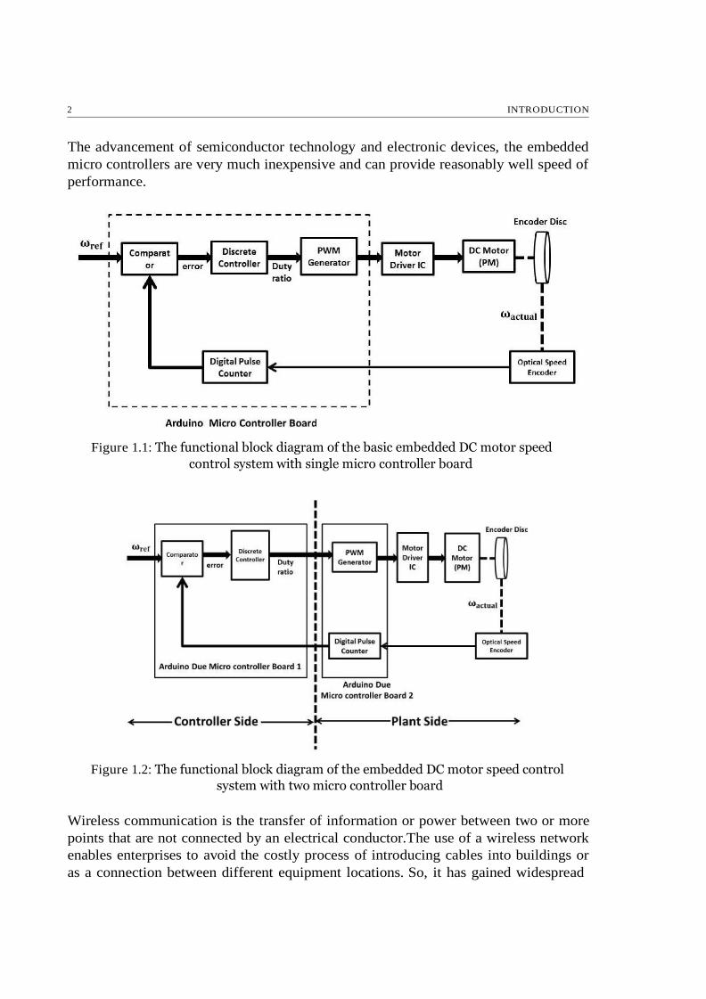
1.1 The functional block diagram of the basic embedded DC motor speed
control system with single micro controller board ................................. 2
1.2 The functional block diagram of the embedded DC motor speed control
system with two micro controller board ................................................... 2
1.3 Wireless networked control systems ........................................................ 3
1.4 Break up of Communication Network Time-delay Into Different Con-
stituents ..................................................................................................... 5
2.1 Waveforms for PWM chopper control of separately excited dc motor. .15
2.2 Arduino UNO board ................................................................................ 16
2.3 Arduino Due Board ................................................................................... 17
2.4 The Bluetooth Module ............................................................................. 18
2.5 The Motor driver IC ................................................................................ 19
2.6 The Speed Encoder With Slotted Disc................................................... 19
2.7 A basic optocoupler unit .......................................................................... 20
2.8 Slots of a speed encoder .......................................................................... 21
2.9 System Identification & the Mode [1] ...................................................... 22
2.10 System Identification Loop [1] ................................................................. 24
2.11 System Identification Toolbox App User Interface ................................. 25
2.12 Data Set for Model Identification ........................................................... 26
2.13 Data Set for Cross Validation of identified Model ................................. 26
2.14 The Circuit Representation of A Permanent Magnet DC Motor [4]. . .30
2.15 The Response of G(s) to the Cross Validation Data .............................. 32
2.16 Step Response of Identified Model G(s) ............................................... 32
2.17 The functional block diagram of the basic embedded DC motor speed
control system with single micro controller board ................................. 34
2.18 The simplified block diagram representation of the DC motor speed con-
trol system ..................................................................................................35
2.19 The simplified s-domain block diagram representation of the DC motor
speed control system ................................................................................ 35
2.20 The SIMULINK block diagram of the closed loop system used in tuning39
2.21 Tuning of the discrete PI controller in MATLAB PID tuner...................40
2.22 The interface of the MATLAB PID tuner ............................................... 40
xi

Contents xii
2.23 The representation of closed loop system in z-domain .......................... 41
2.24 Comparison of system responses with different design strategy for dis-
crete PI controller in SIMULINK ........................................................... 43
2.25 The practical setup for speed control of DC motor (wired fashion). . .44
2.26 Wave forms of the wired speed control setup with discrete PI controller
(with Arduino Due board) ........................................................................45
2.27 Wave forms of the wired speed control setup with discrete PI controller
(with Arduino Uno board)........................................................................ 45
3.1 The Bluetooth Technology Logo .............................................................. 48
3.2 OSI Refernce Model Layers [6] ................................................................. 49
3.3 Functional Blocks in a Bluetooth System [7] ......................................... 50
3.4 The Bluetooth Protocl Stack & Its Mapping with OSI ISO Reference
Model[5,7] .............................................................................................. 53
3.5 Example of data packet exchange in Bluetooth[5] ................................ 55
3.6 The Bluetooth Piconet Topology[5] ........................................................ 56
3.7 The Bluetooth Scatternet Topology[5] ...................................................... 56
3.8 Different States of a Bluetooth Device[1] ............................................... 58
3.9 Connection of an HC-05 module with Arduino Due board ..................... 61
3.10 Connection of an HC-05 module with Arduino Uno board ..................... 62
3.11 Blank sketch uploaded to Arduino board ............................................... 63
3.12 Different pins of HC-05 module ............................................................... 64
3.13 Arduino IDE console while giving AT commands to HC-05 ................. 65
3.14 The functional block diagram of the wireless networked control system
for DC motor speed control .................................................................... 66
3.15 The practical wireless networked system for speed control of DC motor
(point-to-point configuration .................................................................... 66
3.16 The practical wireless networked system for speed control of DC motor
(intermediate node configuration) ........................................................... 67
3.17 The block diagram for testing of Bluetooth network used for control loop68
3.18 The sent and received information at node 1 (point-to-point configuration)68
3.19 Response of the wireless setup with discrete PI controller when τd =
80ms (point-to-point configuration) ................................................ 69
3.20 Response of the wireless setup with discrete PI controller when τd =
240ms (intermediate node configuration) ................................................70
3.21 Response of the wireless setup with discrete PI controller when τd =
300ms (intermediate node configuration) ................................................70
3.22 Response of the wireless setup with discrete PI controller when τd =
400ms (intermediate node configuration) ................................................70
3.23 Graphs for WNCS With Software Defined Serial Ports (point-to-point
configuration) ............................................................................................ 71

Contents xiii
4.1 General block diagram of NCS ................................................................. 74
4.2 Structure of proposed RRT measurement in [1] ...................................... 75
4.3 RTT measurement and delay estimation ............................................... 76
4.4 Structure of RRT measurement for the experimented setup .................. 77
4.5 Measurement and estimation of delay on practical setup ..................... 78
4.6 RTT measurement and delay estimation on practical setup .................. 79
4.7 On line estimated time delays of the practical WNCS system (interme-
diate node configuration ...........................................................................81
4.8 SIMULINK block for comparison of response between the MATLAB
time-delay block & the polynomial series considered ........................... 83
4.9 Step input responses of the MATLAB delay block & different polynomial
series .......................................................................................................... 83
4.10 Block diagram of a typical Smith predictor scheme .............................. 88
4.11 Rearranged form of the typical Smith predictor scheme ........................ 88
4.12 Adaptive self-tuning of a smith predictor scheme for process model mis-
match ........................................................................................................ 90
4.13 Adaptive time delay estimation for smith predictor .............................. 90
4.14 Digital smith predictor structure [19] ...................................................... 91
4.15 Rearranged form of the digital smith predictor represented in figure4.1491
4.16 Data collection in SIMULINK for identification of delay block transfer
function ..................................................................................................... 92
4.17 Implemented digital smith predictor scheme for the wireless point-to-
point configuration ................................................................................... 93
4.18 Practical response and control signal without smith predictor scheme in
wireless point-to-point configuration ........................................................ 93
4.19 Practical response and control signal with smith predictor scheme in
wireless point-to-point configuration ........................................................ 94
4.20 Practical response with smith predictor scheme in network having inter-
mediate nodes (1st time)........................................................................... 94
4.21 Control input with smith predictor scheme in network having interme-
diate nodes (1st time) ............................................................................. 95
4.22 Practical response with smith predictor scheme in network having inter-
mediate nodes (2nd time) ....................................................................... 95
4.23 Control input with smith predictor scheme in network having interme-
diate nodes (2nd time) ............................................................................. 96
4.24 The adaptive digital smith predictor scheme for the wireless network
with intermediate nodes .......................................................................... 97
4.25 Response with Pade series delay approximation of the adaptive digital
smith predictor in wireless network with intermediate nodes ............... 98
4.26 Control input with Pade series delay approximation of the adaptive dig-
ital smith predictor in wireless network with intermediate nodes ......... 98

Contents xiv
4.27 Response with DFR series delay approximation of the adaptive digital
smith predictor in wireless network with intermediate nodes ............... 98
4.28 Control input with DFR series delay approximation of the adaptive dig-
ital smith predictor in wireless network with intermediate nodes ......... 99
4.29 Response of Classical Digital Smith Predictor + PI controller when time
delay = 80 ms......................................................................................... 100
4.30 Response of Classical Digital Smith Predictor + PI controller when time
delay = 240 ms ......................................................................................... 100
4.31 Response of Classical Digital Smith Predictor + PI controller when time
delay = 300 ms ......................................................................................... 101
4.32 Response of Classical Digital Smith Predictor + PI controller when time
delay = 400 ms ......................................................................................... 101
4.33 Response of Adaptive Digital Smith Predictor( DFR approx.) + PI
controller when time delay = 240 ms ................................................. 101
4.34 Response of Adaptive Digital Smith Predictor( DFR approx.) + PI
controller when time delay = 300 ms ................................................. 102
4.35 Response of Adaptive Digital Smith Predictor( DFR approx.) + PI
controller when time delay = 400 ms ................................................. 102
4.36 Response of Adaptive Digital Smith Predictor( Pade approx.) + PI
controller when time delay = 240 ms ................................................. 102
4.37 Response of Adaptive Digital Smith Predictor( Pade approx.) + PI
controller when time delay = 300 ms ................................................. 103
4.38 Response of Adaptive Digital Smith Predictor( Pade approx.) + PI
controller when time delay = 400 ms ................................................. 103
5.1 Nyquist plot(a) & polar plot(b) for the open-loop transfer function G(s)H(s)
without time-delay ................................................................................... 111
5.2 Nyquist plot(a) & polar plot(b) for τd = 0.04s .......................................... 112
5.3 Nyquist plot(a) & polar plot(b) for τd = 0.120s ........................................ 113
5.4 Nyquist plot(a) & polar plot(b) for τd = 0.180s ........................................ 113
5.5 Nyquist plot(a) & polar plot(b) for τd = 0.240s ........................................ 113
5.6 Nyquist plot(a) & polar plot(b) for τd = 0.300s ........................................ 114
5.7 Nyquist plot(a) & polar plot(b) for τd = 0.400s ........................................ 114
5.8 Nyquist plot(a) & polar plot(b) for τd = 0.600s ........................................ 114
5.9 Nyquist plot(a) & polar plot(b) for τd = 1s ........................................... 115
5.10 Nyquist plot(a) & polar plot(b) for τd = 2s........................................... 115
5.11 Polar plot for different time-delays ........................................................ 115

List of Tables
3.1 Different Classes of Bluetooth Radio [4] .................................................. 50
3.2 Different Versions of Bluetooth with Their Speed and Range [4] ......... 60
3.3 Different AT commands used for HC-05 module .................................... 64
4.1 Tabular representation of delay estimation ............................................. 80
4.2 Tabular representation of different delay approximation series ............ 83
4.3 Delay approximation errors .................................................................... 84
5.1 Variation of φM with variation in τd ..........................................................116
xv


Chapter 1
Introduction
DC motor speed controllers are widely used for motion control of robotics, industrial
control and automation systems [8]. Industrial process control has requirements of
adjusting motor speed over a wide range with good resolution and reproducibility
[1]. Conventional analog speed control methods have certain drawbacks, including
nonlinearity in the analog speed transducer and difficulty in accurate transmission of
the analog signal [1]. Also in analog methods signal manipulation suffers from errors
occurring due to temperature, component aging, and external disturbances [1]. In a
digital speed control scheme, there is no nonlinearity associated with speed transducer
and the digital signal of speed can be transmitted to long distances without sacrificing
accuracy [1]. Also in a digital speed control system, the control signal is not adversely
effected by temperature variations, component aging, or noise [1].
For the purpose of speed control of a DC motor, a variable-voltage DC power source
(DC Chopper) is needed [1]. Pulse Width Modulation (PWM) technique is used for
generating variable voltage for speed control purpose [1]. In home appliances the per-
manent magnet DC motor has replaced the ac universal motor due to improve speed
or drive performance [9]. In this research, an embedded speed control method for a
permanent magnet DC motor has been implemented in Arduino Due micro controller
board based on the Atmel SAM3X8E ARM Cortex-M3 CPU. The wired speed control
is done with the help of single Arduino Due micro controller board as shown in fig-
ure2.17. The wired speed control scheme can also be implemented with two Arduino
Due micro controller boards serially connected through wires as in figure1.2.Then the
controller side and plant side of the embedded control system as in figure1.2are con-
nected with an wireless network (Bluetooth) in order to develop a Wireless Networked
Control System (WNCS). The motive of this research is to observe the performance of
the closed loop system with wireless network and then develop necessary techniques or
algorithms for performance improvement if required.
1
2 INTRODUCTION
The advancement of semiconductor technology and electronic devices, the embedded
micro controllers are very much inexpensive and can provide reasonably well speed of
performance.
Figure 1.1: The functional block diagram of the basic embedded DC motor speed
control system with single micro controller board
Figure 1.2: The functional block diagram of the embedded DC motor speed control
system with two micro controller board
Wireless communication is the transfer of information or power between two or more
points that are not connected by an electrical conductor.The use of a wireless network
enables enterprises to avoid the costly process of introducing cables into buildings or
as a connection between different equipment locations. So, it has gained widespread

3
popularity with time and its use keeps growing. Wireless Networked Control System
(WNCS) is a distributed control system with sensor, actuator and controller commu-
nication supported by a wireless network. WNCS can also be defined as a spatially
distributed control system with sensor, actuator and controller communication sup-
ported by a wireless network [19]. WNCSs allow exchange of information among dis-
tributed sensors, controllers actuators over the wireless network to achieve certain
control objectives [19].
Figure 1.3: Wireless networked control systems
The benefits of wireless networked control are [19]:-
1.It is more flexible. Some of the aspects of flexibility are:-
2.Sensors and actuators can be replaced easily.
3.Less restrictive maneuvers and control actions.
4.Powerful control over distributed computations.
5.Reduction in installation and maintenance costs.
6.Requirement of less cabling.
7.Possibility of efficient monitoring and diagnosis.
Wireless technology has some barriers in control and automation. Some of the key
barriers of wireless technology are [19]:
Complexity: Systems designers and programmers need suitable abstractions to
hide the complexity from wireless devices and communication.
Reliability: Systems should have robust and predictable behaviour despite char-
acteristics of wireless networks.
Communication of sensor and actuator data impose uncertainty, disturbances and
constraints on control system.
•
•
•
4 INTRODUCTION
• Communication imperfections in control loops include:
– Time delay and jitter.
– Bandwidth limitations.
– Data loss and bit errors.
– Outages and disconnection.
– Topology variations of different networks.
• Security: Wireless technology is vulnerable to digital hacking or attacks.
There are several approaches to control in WNCS, they are,
Network-aware control: Modify control algorithms to cope with communication
imperfections, for e.g. : predictive controller. In this procedure, in order to adjust
control algorithms, one needs to estimate the network states, like,
– Time Delay
– Data Loss
– Bandwidth
• Control-aware networking: Control of communication resources
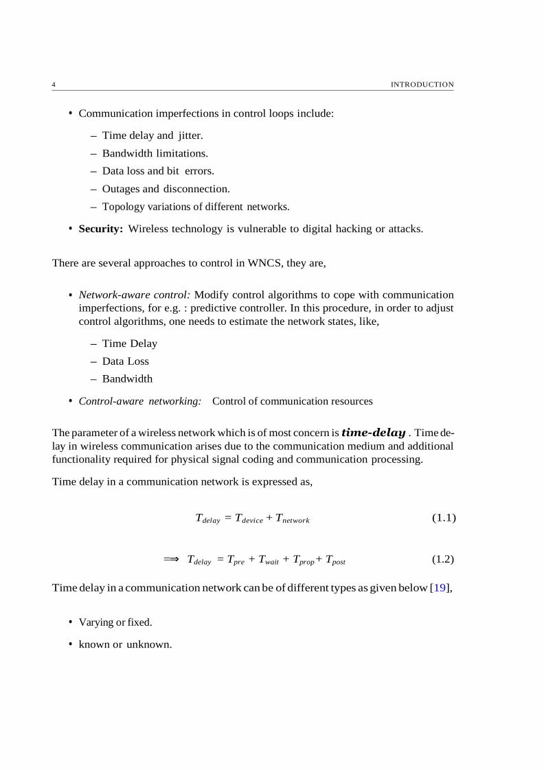
The parameter of a wireless network which is of most concern is time-delay . Time de-
lay in wireless communication arises due to the communication medium and additional
functionality required for physical signal coding and communication processing.
Time delay in a communication network is expressed as,
Tdelay = Tdevice + Tnetwork (1.1)
=⇒ Tdelay = Tpre + Twait + Tprop + Tpost (1.2)
Time delay in a communication network can be of different types as given below [19],
• Varying or fixed.
• known or unknown.
•

1.1. MOTIVATIONS 5
Figure 1.4: Break up of Communication Network Time-delay Into Different Con-
stituents
1.1 Motivations
DC motor drives are widely used in applications requiring adjustable speed control,
frequent starting, good speed regulation, braking and reversing. Some important ap-
plications are paper mills, rolling mills, mine winders, hoists , printing presses, machine
tools, traction, textile mills, excavators and cranes. DC motors are widely used as ser-
vomotors for tracking and positioning. For industrial applications development of high
performance motor drives are very much essential. These applications may demand
high speed control accuracy and good dynamic response. Some other examples of DC
motor speed control applications are washers, dryers and other household appliances.
Applications of DC motor speed control are also found in the automotive area for uses
such as fuel pumps, electronic steering, and engine controls.DC motor drives are less
costly and less complex compared to AC motor drives. Moreover, use of embedded
systems for speed control purpose of DC motor brings the cost to much lower value.
Development of very low cost embedded speed control system can also serve as a good
laboratory experiment to understand and learn control engineering practically.
Motivating applications of Wireless Networked Control Systems (WNCSs) are as fol-
lows,
Wireless Process Control Industrial Automation: Communication cabling
is subject to heavy wear and tear in industrial controlled processes & robots and
therefore requires frequent maintenance. This implies increased maintenance cost.
Replacing cables or wires with wireless network saves cost
Medical Applications: For example, Glucose-Insulin monitoring & control of
Diabetic Patient.
Practical Fault Tolerant System: WNCSs are tolerant to sensor controller
failure. If a sensor or controller fails, the system can use that of any other
connected system within the wireless network.
•
•
•

6 INTRODUCTION
1.2 Problem Statement
In this thesis, design of a closed-loop DC motor (permanent magnet) servo system for
speed control will be discussed. Then implementation of the servo system using an
embedded system platform (Arduino micro controller board) will be explained. The
controller will be a discrete PI controller. Then the servo system will be distributed into
two parts : controller side (containing reference input functionality, discrete controller
and comparator) and plant side containing (actuator, sensor and the DC motor plant),
with both the parts connected through a Bluetooth wireless network. The behaviour
of the wireless network in the control loop will be examined. Then the performance of
the servo system with the wireless network will be observed. After that measurement,
estimation and approximation of the network parameters effecting the performance of
the servo system will be discussed in detail. Based on the estimated wireless network
parameters (e.g. time delay) , predictive control strategies will be developed for bet-
ter performance of the servo system. Then the implementation of predictive control
strategies in embedded platform will be discussed.
1.3 Literature Review
DC motor speed control problem is an age old problem that scientists and researchers
are dealing with. There are lots of papers available in literature on DC motor speed
control using various analog techniques and power electronic methods. Maloney, T.J.
and Alvarado, F.L. (1976) [1] first discussed a digital method for DC motor speed
control where digital tachometer was used to remove the nonlinearity associated with
analog transducers. A. K. Lin and W. W. Koepsel (1977) [2] first discussed a mi-
croprocessor (Intel 8080) based speed control strategy using DC chopper to achieve
reasonably low steady state error. J. B. Plant and S. J. Jorna (1980) [3] published an
SCR based dc motor drive control where a microprocessor performed both the control
law computation and logical functions of SCR. State space methodology was used for
the control purpose and stability, error analysis of the controller was provided. A. H.
M. S. Ula, J. W. Steadman and J. M. Wu (1988) [4] explained a micro controller based
speed control for industrial size DC motor using thyristors. J. Nicolai and T. Castagnet
(1993) [5] discussed a permanent magnet DC motor speed control using micro controller
generated PWM signal. Software flexibility for modifying drive parameters like maxi-
mum power, time constant etc. were also explained in that paper. T. Castagnet and
J Nicolai (1994) [9] discussed a micro controller based brush DC motor speed control
through direct voltage compensation and motor power limitation. Y. S. E. Ali, S. B.
M. Noor, S. M. Uashi and M. K. Hassan (2003) [6] explained a micro controller based
speed control and over current protection scheme for a DC motor. These are the key
publications found in literature on embedded/ micro controller/ microprocessor based
DC motor servo systems.

1.3. LITERATURE REVIEW 7
There are a large number of publications on networked control systems, but the num-
ber of research in wireless networked control systems are less in number [11]. J. Eker,
A. Cervinnad A. Hrjel (2001) [10] discussed a distributed control method using Blue-
tooth network and provided solution for two specific problems occurring while using
Bluetooth in a control loop: long random delays and bit errors. N. J. Ploplys, P. A.
Kawka and A.G. Alleyne (2004) [11] developed a method for near real-time control
over a wireless network and implemented for a practical set up. It has been found that
The use of event-driven control with clock driven sensing and actuation gives a natu-
ral synchronization of the control loop without clock synchronization of the individual
nodes [11]. Y. Jianyong, Y. Shimin and W. Haiqing (2004) [11] published survey on
the performance analysis of Networked Control Systems (NCSs) where main aspects
around performance analysis of NCSs were: network-induced delays, sampling period,
jitter, data pocket dropout, network scheduling and stability. C.H. Chen, C.L. Lin and
T.S. Hwang (2007) [14] showed that stability of the closed-loop system is guaranteed up
to some maximum upper bound of the round trip delay. J. De Boeij, M. Haazen and P.
Smulders (2009) [17] presented a new approach for wireless motion control with a new
protocol and wireless system that reduce the closed loop transmission delay to less than
300 microseconds. The system was verified in a real control system, and measurements
showed the performance, which was more than ten times better than existing tech-
niques. A. Hernandez (2010) [13] discussed use of IEEE 802.15.4 wireless protocol in
control applications. An inverted pendulum process is introduced to show the benefits
in wireless process control by using the IEEE 802.15.4 (as wireless sensor network) in
a real-time control loop process. The extensive experimental results show that packets
losses and delays are the essential factors to guarantee the stability of the system. C.L.
Lai and P.L. Hsu (2010) [15] discussed a networked remote control system (wired) and
online measurement of the round-trip time (RTT) between the application layers of the
server and the client. M. Pajic, S. Sundaram, G. Pappas and R. Mangharam (2011) [16]
presented a distributed scheme used for control over wireless networks, where where
the network itself, with no centralized node, acts as the controller. C. Suryendu, S.
Ghosh and B. Subudhi (2017) [18] discussed a gradient descent method based delay
estimator for use with a variable gain control strategy for wireless networked control
systems. The delay estimator was developed in such a way that its boundedness is
ensured. The performance of the estimator with variable gain controller was evaluated
on a temperature control plant with network in the feedback loop. From the literature
survey on WNCS/NCS applications, we have found that most of the works are done
using PCs, high performance computers and hence cost of implementation goes high.
We could not find any literature to discuss WNCS implementation using embedded
hardware platform.
For compensation of time delays occurring in control systems, predictive control strate-
gies need to be adopted for compensation of time delays. Smith predictor is one of the
most popular scheme for time delay compensation. In 1957 O.J. Smith first proposed
the smith predictor scheme to compensate time delays occurring in process control

8 INTRODUCTION
applications. Since then it has become one of the most popular dead time compen-
sation scheme and many papers have been published. D. E. Lupfer, M. W. Oglesby
(1962) discussed an implementation of smith predictor in automatic process control.
Alevisakis & Seborg (1973) extended smith predictor to multivariable systems with
single delay and that to multivariable systems with multiple delays by Ogunnaike &
Ray (1979). C. Meyer, .D.E. Seborg & R.K. Wood (1976) gave a comparison of smith
predictor and conventional PI control scheme having dead time both in forward and
feedback path in simulation.JR Schleck & D Hanesian (1978) evaluated linear smith
predictor structure for dead time dominating process. A. C. Ioannides, G. J. Rogers
& V. Latham (1978) discussed stability limits of smith predictor controller for simple
systems when process-model mismatch occurs. C. Meyer, .D.E. Seborg & R.K. Wood
(1979) also provided a comparison between analytical predictor and smith predictor
scheme. Z. Palmor (1980) also investigated the stability properties of smith time de-
lay compensator scheme with practical conditions of stability. A. Terry Bahill (1983)
published a tutorial on simple smith predictor scheme with adaptive nature to process
parameter variation. Wellons and Edgar (1985) discussed a Generalized Analytical
Predictor (GAP) for dead time systems and its relationship with smith predictor, IMC
strategy and discrete analytical predictor in simulation. Z. J. Palmor and D. V. Powers
(1985) proposed a modified smith predictor with simultaneous feedforward & feedback
actions with a control on degree of dead time compensation.S. K. P. Wong and D. E.
Seborg (1986) gave a theoretical analysis of smith predictor and analytical predictors.
Until 1980, smith predictor schemes developed were mostly analog & hence were not
used in the industry due complexity of analog technique. Vogel, E. F. and T. F.
Edgar, in 1980, proposed a digital control scheme for dead time compensation. In
the same year, they also proposed adaptive control strategies for variable dead time
compensation in simulation level. C. C. Hang, K. W. Lim & T. T. Tay (1986) also
proposed an adaptive digital scheme of smith predictor in simulation. An adaptive
digital smith predictor with dual rate sampling, i.e. smaller sampling time for control
& larger sampling time for on-line parameter estimation, have been discussed by C.
C. Hang, K. W. Lim and B. W. Chong (1989). Many researchers discussed modified
smith predictor for system with integrator and long dead time and some of them are
K.J. Astrom and Hang Lim (1994), M.R. Matausek and A. D. Micric (1996), J. E.
Normey-Rico and E.F. Camacho (1999). V Massimiliano (2003) gave a improved smith
predictor structure through automatic dead time computation in practical. Chen Peng,
Dong Yue & Ji Sun (2004) proposed smith predictor structure in Networked Control
System (NCS) employing on-line time delay identification and provided simulation
results. Chun-Hsiung Chen, Chun-Liang Lin, and Thong-Shing Hwang (2007) discussed
a robust smith predictor to compensate varying round trip delay time in NCS and
the maximum upper bound of the round trip delay providing guaranteed stability in
simulation. Chien-Liang Lai and Pau-Lo Hsu (2010) discussed a method for on line
measurement of round trip delay time in NCS and based on that round trip delay time
an adaptive smith predictor scheme was proposed for a servo system in practical. Rui
Wang, Guo-Ping Liu, Wei Wang, David Rees, and Yunbo B. Zhao (2010) proposed an
1.4. THESIS OUTLINE 9
improved predictive controller design strategy for NCS to compensate for the varying
time delay and data dropout in both the forward and backward channels to achieve
the desired control performance. V Bobl, P Chalupa and P Dostl (2010) proposed
a digital adaptive smith predictor based on pole assignment or polynomial design in
simulation. V Bobl, P Chalupa, P Dostl and M Kubalk (2014) again proposed a digital
smith predictor for control of unstable and integrating time-delay processes.
From the literature review, it has been found that most of the publications discussed
simulation study of various smith predictor strategies for time delayed systems. Very
few of them mentioned about practical implementation (e.g. V Massimiliano (2003),
Chien-Liang Lai and Pau-Lo Hsu (2010)). Although all of the practical implementa-
tions found in literature were done using sophisticated computing systems and we could
hardly find any paper that discusses real time embedded system application. There
are a handful amount of work on smith predictor strategy for NCS, but we could not
find any publication that provides practical implementation for Wireless Networked
Control System in embedded platform.
1.4 Thesis Outline
The thesis is divided into 7 chapters as follows,
Chapter 1: It discusses an introduction to embedded speed control of DC motor
and Wireless Networked Control Systems (WNCSs). Also motivations for work,
problem statement and literature review has been presented.
Chapter 2: This chapter provides DC motor plant description, speed control
methodology, modeling and system identification of the plant, discretization of
the system and design of discrete PI controller. Then practical implementation
of the servo system is discussed.
Chapter 3: This chapter deals with details on Bluetooth communication tech-
nology, behaviour of the Bluetooth network to be used in control loop, develop-
ment and implementation of WNCS for the DC motor servo system.
Chapter 4: This chapter discusses time delay measurement, estimation and
approximation in the WNCS. Practical embedded implementation for time delay
estimation as RTT (Round Trip Time) has been discussed. Then time delay
compensation using digital Smith Predictor in Arduino embedded platform for
fixed and varying time delays in the wireless network is presented.
Chapter 5: This chapter gives an stability analysis of the DC motor plant with
time delay.
•
•
•
•
•

10 REFERENCES
Chapter 6: This chapter discusses modifications from existing literature adopted
in the practical WNCS set up and contributions or proposal of the research.
• Chapter 7: This chapter provides conclusions and future works.
1.5 Chapter Summary
In this chapter basic idea about the embedded platform based speed control system for
a PMDC motor has been provided. We have also discussed introductory ideas about
WNCSs. Then motivations and problem definition are provided. Literature survey
related to the research work presented in the thesis has also been provided.
References
[1] Maloney, T.J. and Alvarado, F.L., 1976. A digital method for dc motor speed
control.IEEE Transactions on Industrial Electronics and Control Instrumentation,
(1), pp.44-46.
[2] Lin, A.K. and Koepsel, W.W., 1977. A microprocessor speed control system. IEEE
Transactions on Industrial Electronics and Control Instrumentation, (3), pp.241-
247.
[3] Plant, J.B., Jorna, S.J. and Chan, Y.T., 1980. Microprocessor control of position
or speed of an SCR dc motor drive. IEEE Transactions on Industrial Electronics
and Control Instrumentation, (3), pp.228-234.
[4] Ula, A.H.M.S., Steadman, J.W. and Wu, J.M., 1988. Design and demonstration of
a microcomputer controller for an industrial sized DC motor. IEEE transactions on
energy conversion, 3(1), pp.102-110.
[5] Nicolai, J. and Castagnet, T., 1993, September. A flexible micro-controller based
chopper driving a permanent magnet DC motor. In Power Electronics and Appli-
cations, 1993., Fifth European Conference on (pp. 200-203). IET.
[6] Ali, Y.S.E., Noor, S.B.M., Bashi, S.M. and Hassan, M.K., 2003, December. Micro-
controller performance for DC motor speed control system. In Power Engineering
Conference, 2003. PECon 2003. Proceedings. National (pp. 104-109). IEEE.
[7] Dewangan, A.K., Chakraborty, N., Shukla, S. and Yadu, V., 2012. PWM based au-
tomatic closed loop speed control of DC motor. international journal of engineering
trends and technology, 3(2), pp.110-112.
•

REFERENCES 11
[8] Mathur, A., 2008. Microcontroller-Based DC Motor Speed Controller Electronics
For You, 2009.
[9] Castagnet, T. and Nicolai, J., 1994. Digital control for brush DC motor. IEEE
transactions on industry applications, 30(4), pp.883-888
[10] Eker, J., Cervin, A. and Hrjel, A., 2001. Distributed wireless control using Blue-
tooth. IFAC Proceedings Volumes, 34(22), pp.360-365.
[11] Ploplys, N.J., Kawka, P.A. and Alleyne, A.G., 2004. Closed-loop control over
wireless networks. IEEE control systems, 24(3), pp.58-71.
[12] Jianyong, Y., Shimin, Y. and Haiqing, W., 2004, October. Survey on the perfor-
mance analysis of networked control systems. In Systems, Man and Cybernetics,
2004 IEEE International Conference on (Vol. 6, pp. 5068-5073). IEEE.
[13] Hernndez Herranz, A., 2010. Wireless Process Control using IEEE 802.15. 4 Pro-
tocol.
[14] Chen, C.H., Lin, C.L. and Hwang, T.S., 2007. Stability of networked control sys-
tems with time-varying delays. IEEE Communications Letters, 11(3).
[15] Lai, C.L. and Hsu, P.L., 2010. Design the remote control system with the time-
delay estimator and the adaptive smith predictor. IEEE Transactions on Industrial
Informatics, 6(1), pp.73-80.
[16] Pajic, M., Sundaram, S., Pappas, G. and Mangharam, R., 2011. A simple dis-
tributed method for control over wireless networks.
[17] De Boeij, J., Haazen, M., Smulders, P. and Lomonova, E., 2009. Low-latency wire-
less data transfer for motion control. Journal of Control Science and Engineering,
2009, p.3.
[18] Suryendu, C., Ghosh, S. and Subudhi, B., 2017. Variable Gain Output Feedback
Control of A Networked Temperature Control System Based on Online Delay Esti-
mation. Asian Journal of Control.
[19] Johansson, K. H., 2006. Control over Wireless Networks: Research Challenges and
Case Studies. GRASP Seminar Series University of Pennsylvania, Philadelphia
[20] Bobl, V., Chalupa, P., Dostl, P. and Kubalk, M., 2014. Digital Smith Predictor
for Control of Unstable and Integrating Time-delay Processes. In Proceedings of
the 2014 international conference on mechatronics and robotics, structural analysis
(MEROSTA 2014), Santorini Island, Greece (pp. 105-110).
[21] Bobl, V., Matunu, R. and Dostl, P., 2011, June. Digital Smith Predictors-Design
And Simulation Study. In ECMS (pp. 480-486).
12 REFERENCES
[22] Bobl, V., Chalupa, P., Dostl, P. and Kubalk, M., 2011, May. Adaptive digital
Smith predictor. In Recent Researches in Automatic Control-13th WSEAS Interna-
tional Conference on Automatic Control, Modelling and Simulation, ACMOS’11.
[23] O’Dwyer, Aidan : A reference guide to Smith predictor based methods for the
compensation of dead-time processes. Proceedings of the IEE Irish Signals and Sys-
tems Conference, pp. 231-238, Dublin City University, September, 2005.
[24] Sourdille, Pauline and O’Dwyer, Aidan : An outline and further development of
Smith predictor based methods for the compensation of processes with time delay.
Proceedings of the Irish Signals and Systems Conference, pp. 338-343, University of
Limerick, July, 2003.
[25] Bahill, A., 1983. A simple adaptive smith-predictor for controlling time-delay sys-
tems: A tutorial. IEEE Control systems magazine, 3(2), pp.16-22.
[26] Deshpande, P. B. and Ash, R. H., 1981. Elements of Computer Process Control
With Advanced Control Applications. Research Triangle Park NC: Instrument So-
ciety of America, 1981. pp. 227-250.

Chapter 2
Plant Modeling, Controller Design
and The Practical DC Motor Speed
Control System
There are various types of speed control methods used for DC motor’s speed control.
In our experiment, the DC motor is of permanent magnet type i.e.separately excited.
Various speed control methods used for DC separately excited motors are[5]:
• Armature Voltage Control Method
• Armature Resistance Control Method
• Field Control Method
In our case, we are going with armature voltage control due to the following reasons:
Field control method is not application as the DC motor used is of permanent
magnet type.
• Rotor resistance control method suffers from extra power loss.
Armature voltage control is preferred because of high efficiency, good transient
response and good speed regulation.
13
•
•

PLANT MODELING, CONTROLLER DESIGN AND THE PRACTICAL DC MOTOR SPEED CONTROL
SYSTEM 14
⇒
2.1 Armature Voltage Control For Speed Regula-
tion
It is the method by which the speed of a DC motor is controlled by giving variable
input armature voltage to the motor. The motor we use here is a permanent magnet
separately excited dc motor therefore the field flux φ is constant.
Therefore, back emf of motor E = Kω, where ω is the speed of the motor K is back
emf constant.
Now, for V being terminal voltage, Ia being the armature current, R being the armature
resistance, the back emf of the motor is given as[5]:-
E = Kω = V − IaR (2.1)
= ω = V − IaR
K
(2.2)
Therefore, from equation2.2, we can see that by varying the voltage V, we can vary
the speed of the motor.
There are various methods by which armature voltage control can be done.
When the supply is ac, we can use [5]:
• Ward-Leonard schemes
• Transformer with taps and an uncontrolled bridge rectifier
• Static Ward-Leonard scheme or controlled rectifiers
As we are using a dc supply,the pulse width is varied using Pulse Width Modulation
(PWM) technique. It is a chopper control strategy to produce variable voltage from a
fixed voltage.
2.1.1Chopper Control of Separately Excited dc Motors
The waveform of a PWM (Pulse Width Modulation) chopper device used for DC motor
speed control is shown in figure2.1The frequency of PWM scheme should be high to
ensure continuous conduction[5].
The waveform is given as:-

2.2. HARDWARE COMPONENTS USED 15
Figure 2.1: Waveforms for PWM chopper control of separately excited dc motor
Ratio of duty interval ton to chopper period T is called duty ratio or duty cycle (δ).
Thus [5]
δ = Dutyinterval
= ton (2.3)
T t
Va = δV (2.4)
Now as [5],
I = δV − E
a R
(2.5) a
From equations2.2and2.5 δV
ωm = K
RaT
− K2
(2.6)
In this way the speed of a DC motor with permanent magnet poles can be controlled.
2.2Hardware Components Used
2.2.1Arduino Micro Controller Board
Arduino is an open source hardware and software project first introduced in 2005 aiming
to provide an accessible way for novices and professionals to create devices that interact
with their environment using sensors and actuators. Common examples of such devices
include simple robots, thermostats, and motion detectors.
PLANT MODELING, CONTROLLER DESIGN AND THE PRACTICAL DC MOTOR SPEED CONTROL
SYSTEM 16
Arduino is based on micro controller board designs, which use inputs and outputs in
the same way an ordinary computer does. Inputs capture information from the user
or the environment while outputs do something with the information that has been
captured. An input could be digital or analog, and could come from the environment
or a user. Outputs can control and turn on and off devices such as motors or other
computers. These systems provide sets of digital and analog input/output (I/O) pins
that can interface to various expansion boards (termed shields) and other circuits. The
boards feature serial communication interfaces, including Universal Serial Bus (USB)
on some models, for loading programs from personal computers.
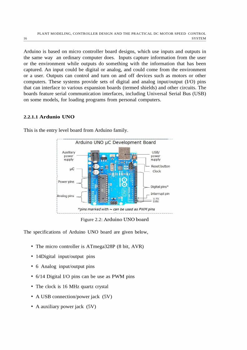
2.2.1.1 Ardunio UNO
This is the entry level board from Arduino family.
Figure 2.2: Arduino UNO board
The specifications of Arduino UNO board are given below,
• The micro controller is ATmega328P (8 bit, AVR)
• 14Digital input/output pins
• 6 Analog input/output pins
• 6/14 Digital I/O pins can be use as PWM pins
• The clock is 16 MHz quartz crystal
• A USB connection/power jack (5V)
• A auxiliary power jack (5V)

2.2. HARDWARE COMPONENTS USED 17
• Flash Memory 32 KB
• SRAM 2 KB
• EEPROM 1 KB
• One Serial Transmitter (Tx)
• One Serial Receiver (Rx)
2.2.1.2 Arduino Due
This is one of the most advanced Arduino boards.
Figure 2.3: Arduino Due Board
The specifications of Arduino Due board are given below,
• Atmel SAM3X8E ARM Cortex-M3 CPU (32-bit)
• 54 Digital input/output pins
• 12 PWM pins among the 54 digital I/O pins.
• 12 analog input pins.
• The clock is 84 MHz quartz crystal.
• A USB connection and power jack (5V).
• 2 DAC pins.

PLANT MODELING, CONTROLLER DESIGN AND THE PRACTICAL DC MOTOR SPEED CONTROL
SYSTEM 18
−
• Flash Memory 512 KB.
• SRAM 96 KB
• EEPROM 1 KB
• 4 UART transmitter-receiver pin pairs.
2.2.2 The Bluetooth module
Bluetooth is a wireless technology standard for exchanging data over short distances
using short-wavelength UHF radio waves. The model we are using is HC 05 Bluetooth
Serial Port Protocol (SPP) Module.
Figure 2.4: The Bluetooth Module
Specifications:
• Bluetooth V2.0+EDR (Enhanced Data Rate)
• 3 Mbps Data Rate
• 2.4GHz radio transceiver and baseband
• Low Power 1.8V Operation ,1.8 to 3.6V I/O
• Supported baud rate: 9600,19200,38400,57600,115200,230400,460800
• Data bits:8, Stop bit :1, No Parity.
2.2.3 The Motor Driver IC
Motor drivers act as current and/or voltage amplifiers since they take a low-current
and/or low-voltage control signal and provide a higher-current signal. This higher
current signal is used to drive the motors. The Motor Drive IC used is L-293D.

2.3. SPEED MEASUREMENT BY OPTICAL ENCODER 19
Figure 2.5: The Motor driver IC
2.2.4 The Optical Speed Encoder
• Model : HC-020k Module with Opto-coupler unit.
• Slotted Encoder Disc (20 slots)
• Measurement frequency: 100 KHz
• Module Working Voltage: 4.5-5.5V
• Encoder resolution: 20 lines
Figure 2.6: The Speed Encoder With Slotted Disc
2.3 Speed Measurement by Optical Encoder
The optical speed encoder consists of two parts:
• An optical encoder or optocoupler unit.
• A slotted encoder disc.

PLANT MODELING, CONTROLLER DESIGN AND THE PRACTICAL DC MOTOR SPEED CONTROL
SYSTEM 20
2.3.1 Optocoupler
An Optocoupler, also known as an Opto-isolator or Photo-coupler, is an electronic
component that transfers electrical signals between two electrical circuits with the help
of light. The main purpose of opto-coupler is to provide isolation between two electrical
circuits.
An opto-isolator connects input and output sides with a beam of light modulated by
input current. It transforms useful input signal into light, sends it across the dielectric
channel, captures light on the output side and transforms it back into electric signal.
A basic optoisolator consists of a light-emitting diode (LED), IRED (infrared-emitting
diode) or laser diode for signal transmission and a photosensor (or phototransistor) for
signal reception. Using an optocoupler, when an electrical current is applied to the
LED, infrared light is produced and passes through the material inside the optoisola-
tor. The beam travels across a transparent gap and is picked up by the receiver, which
converts the modulated light or IR back into an electrical signal. In the absence of
light, the input and output circuits are electrically isolated from each other.
Figure 2.7: A basic optocoupler unit
Electronic equipment, as well as signal and power transmission lines, are subject to
voltage surges from radio frequency transmissions, lightning strikes and spikes in the
power supply. To avoid disruptions, optoisolators offer a safe interface between high-
voltage components and low-voltage devices.
A circuit breaker performs the same function in many electrical circuits but if fault
2.3. SPEED MEASUREMENT BY OPTICAL ENCODER 21
persists, then the circuit will trip which disrupts the continuity of flow. The optocou-
pler will simply block the transient due to fault and passes the normal signal.
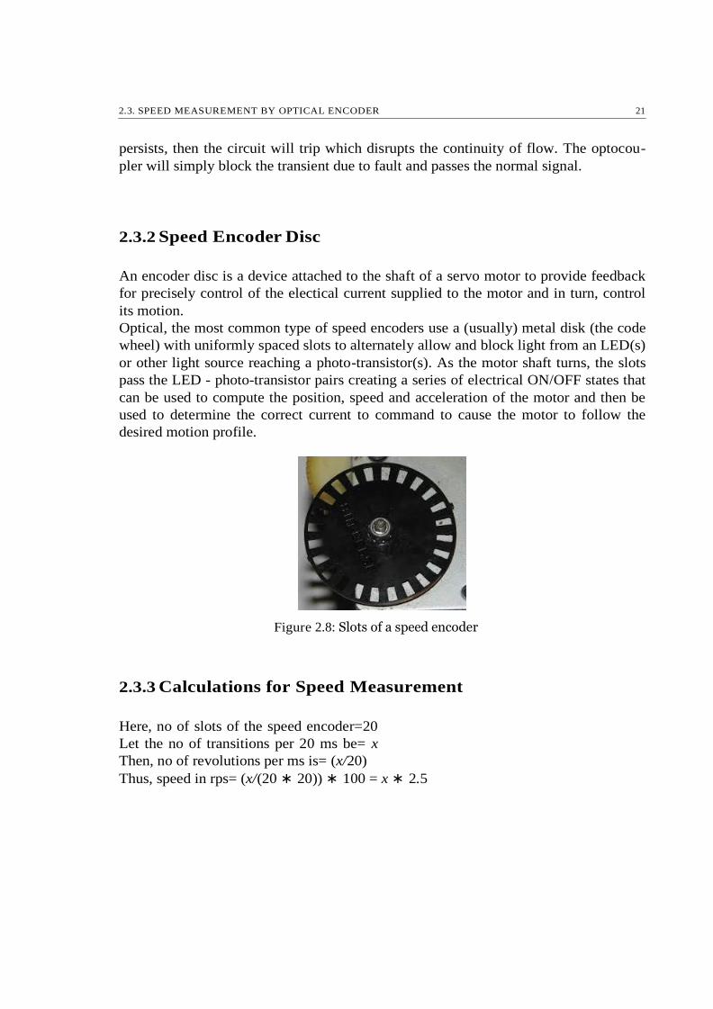
2.3.2 Speed Encoder Disc
An encoder disc is a device attached to the shaft of a servo motor to provide feedback
for precisely control of the electical current supplied to the motor and in turn, control
its motion.
Optical, the most common type of speed encoders use a (usually) metal disk (the code
wheel) with uniformly spaced slots to alternately allow and block light from an LED(s)
or other light source reaching a photo-transistor(s). As the motor shaft turns, the slots
pass the LED - photo-transistor pairs creating a series of electrical ON/OFF states that
can be used to compute the position, speed and acceleration of the motor and then be
used to determine the correct current to command to cause the motor to follow the
desired motion profile.
Figure 2.8: Slots of a speed encoder
2.3.3 Calculations for Speed Measurement
Here, no of slots of the speed encoder=20
Let the no of transitions per 20 ms be= x
Then, no of revolutions per ms is= (x/20)
Thus, speed in rps= (x/(20 ∗ 20)) ∗ 100 = x ∗ 2.5

PLANT MODELING, CONTROLLER DESIGN AND THE PRACTICAL DC MOTOR SPEED CONTROL
SYSTEM 22
2.4 System Identification
System Identification is the process of building or describing a relationship between
the input & output of a system or process from observed or measured data [1]. System
identification is a statistical methods in control system engineering to build mathemat-
ical and analytical models of dynamic systems from the already inferred data .It is an
experimental or empirical Modeling technique [1].
Model is the relationship among cause-effect signals and it provides a description of
the system. Models serve as good mathematical substitutes for the system. To infer a
model, input and output signals from the system are recorded and analysed [1].
Figure 2.9: System Identification & the Mode [1]
2.4.1 Purpose of System Identification
The main purposes of using system identification are as follows [1]:
• To obtain a mathematical model for controller design.
• To explain or understand observed phenomena
• To forecast events in future.
• To obtain a model of signal in filter design.
2.4.2 Different Approaches For System Identification
There are two types of approach for system identification [1]:

2.4. SYSTEM IDENTIFICATION 23
1. Non-parametric Approach : Non-parametric approach gives basic idea about
the system is useful for validation. A good estimate of time delay is provided &
some insights to order of the process along with other variable information such as
time constants, presence of integrators, inverse response is found. This approach
aims at determining a time or frequency response directly without first selecting
a possible set of models. A structure &the order of the parametric model is found
using the information gathered from non-parametric model. Three most common
non-parametric models are:
• Finite Impulse Response (FIR) Model.
• Step Response Model
• Frequency Response Model
2. Parametric Approach : Assumptions on model structure is required in the
parametric approach. It becomes more complicated than non-parametric ap-
proach as the search for the best model within the candidate set becomes a
problem of determining the model parameters. The various types of parametric
models are:
• Auto-Regressive Exogenous (ARX).
• Auto-Regressive Moving Average (ARMAX)
• Output Error (OE)
• Box-Jenkins Model(BJ)
• State Space Model.
2.4.3 Systematic Procedure for Identification
The construction of model from input-output data involves the following basic entities
[1]:
1. The Data : There may be two possibilities: Specially designed identification ex-
periment, where user may determine which signals to measure & when to measure
them & may also choose the input signals or the user may not have the possibil-
ity to affect the experiment, but must use data from the normal operation of the
system.
2. A Set of Candidate Models : By specifying within which the collection of
models we are going to look for a suitable one, a set of candidate models is
obtained. Then a model with some unknown physical parameters is developed
from basic physical laws other well established relationships. In other cases two
types of linear models can be employed:
PLANT MODELING, CONTROLLER DESIGN AND THE PRACTICAL DC MOTOR SPEED CONTROL
SYSTEM 24
Black Box Model: Models set with adjustable parameters with no physical
interpretation.
Grey Box Model: Model set with adjustable parameters with physical
interpretation
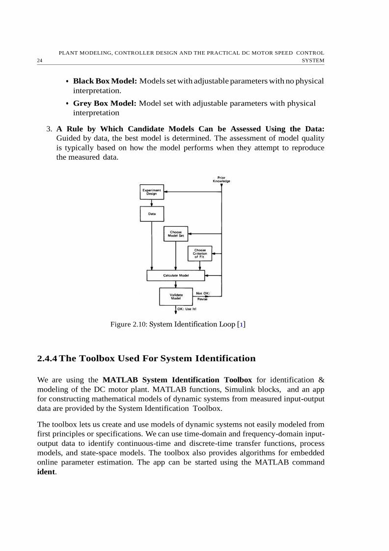
3. A Rule by Which Candidate Models Can be Assessed Using the Data:
Guided by data, the best model is determined. The assessment of model quality
is typically based on how the model performs when they attempt to reproduce
the measured data.
Figure 2.10: System Identification Loop [1]
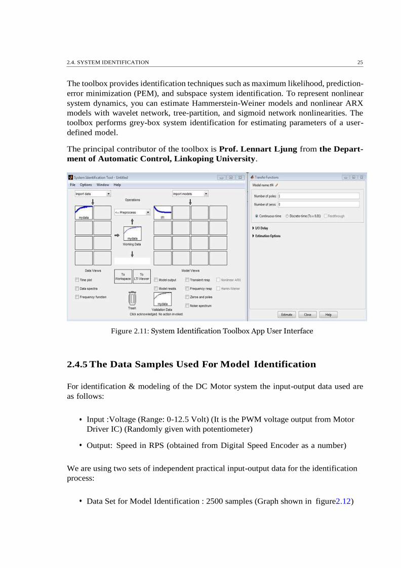
2.4.4 The Toolbox Used For System Identification
We are using the MATLAB System Identification Toolbox for identification &
modeling of the DC motor plant. MATLAB functions, Simulink blocks, and an app
for constructing mathematical models of dynamic systems from measured input-output
data are provided by the System Identification Toolbox.
The toolbox lets us create and use models of dynamic systems not easily modeled from
first principles or specifications. We can use time-domain and frequency-domain input-
output data to identify continuous-time and discrete-time transfer functions, process
models, and state-space models. The toolbox also provides algorithms for embedded
online parameter estimation. The app can be started using the MATLAB command
ident.
•
•
2.4. SYSTEM IDENTIFICATION 25
The toolbox provides identification techniques such as maximum likelihood, prediction-
error minimization (PEM), and subspace system identification. To represent nonlinear
system dynamics, you can estimate Hammerstein-Weiner models and nonlinear ARX
models with wavelet network, tree-partition, and sigmoid network nonlinearities. The
toolbox performs grey-box system identification for estimating parameters of a user-
defined model.
The principal contributor of the toolbox is Prof. Lennart Ljung from the Depart-
ment of Automatic Control, Linkoping University.
Figure 2.11: System Identification Toolbox App User Interface
2.4.5 The Data Samples Used For Model Identification
For identification & modeling of the DC Motor system the input-output data used are
as follows:
Input :Voltage (Range: 0-12.5 Volt) (It is the PWM voltage output from Motor
Driver IC) (Randomly given with potentiometer)
• Output: Speed in RPS (obtained from Digital Speed Encoder as a number)
We are using two sets of independent practical input-output data for the identification
process:
• Data Set for Model Identification : 2500 samples (Graph shown in figure2.12)
•

PLANT MODELING, CONTROLLER DESIGN AND THE PRACTICAL DC MOTOR SPEED CONTROL
SYSTEM 26
Data Set for cross validation of identified model : 998 samples (Graph shown in
figure2.13).
The sampling time for each data set is selected as 20ms.
It is important to note the the input-output data sets are normalized to values (0-1)
during identification process and the normalization is done using formula,
x = x − xmin (2.7)
norm xmax − xmin
Where, x is any data point in the input-output data set.
Figure 2.12: Data Set for Model Identification
Figure 2.13: Data Set for Cross Validation of identified Model
2.4.6 Linear Least-Squared Error Minimization for System
Identification
It is a technique used for minimizing errors during System Identification. It is also
called Prediction Error Minimization [1].
•

2.4. SYSTEM IDENTIFICATION 27
Σ Σ
1 2 1 2
For simplicity let us take a simple ARX(221) (Auto Regressive Exogeneous Input with
na = 2, nb = 2nk = 1) model (equation-error structure) consisting of 2 input & 2 output
parameters as [1],
A(q)y(t) = B(q)u(t) + e(t) (2.8)
Where, y(t) is the output signal, u(t) is the input signal & e(t) is the error signal or
white noise [1].
Here, A(q) = 1 + a1q
−1 + a2q
−2 (2.9)
B(q) = b1q−1
+ b2q−
2 (2.10)
Where, q
−1 is the delay or shift operator i.e. q
−lx(t) = x(t − l)
The transfer function of the plant when mean squared error is zero or minimum is given
as [1],
G(q) = B(q)
A(q) (2.11)
It has been assumed that B(q) & A(q) has no factor in common.
Now,from equation2.8we can write the equation of the system as [1],
y(t) = −a1y(t − 1) − a2y(t − 2) + b1u(t − 1) + b2u(t − 2) + e(t) (2.12)
Now, from equation2.12, we can define a linear regressor matrix as [1],
Φ = −y(t − 1) −y(t − 2) u(t − 1) u(t − 2)
Also, we define parameter matrix as [1],
θ = Σ
a a b b ΣT
Now from equation2.12we get,
e(t) = y(t) − Φθ (2.13)
Now, we have to minimize e2(t) by using the regressor matrix, therefore we define a
objective function J(θ) as [1],
J(θ) = e2(t) = [y(t) − Φθ]
T (2.14)
PLANT MODELING, CONTROLLER DESIGN AND THE PRACTICAL DC MOTOR SPEED CONTROL
SYSTEM 28
−
Now, gradient of J is given as,
∂J(θ) = 2Φ
T y + 2Φ
T Φθ (2.15)
∂θ
The least squared error will be minimum when the gradient of J is zero, which gives,
θ = (ΦT Φ)
−1Φ
T y(t) (2.16)
Now this parameters of equation2.16obtained by least square estimation give us the
transfer function of the plant. Here, the estimation is done in terms of the parameters
in the continuous time system which are sampled to match the observed data.
2.4.7 Nonlinear Least-Squared Error Minimization for System
Identification
This technique is used by the MATLAB System Identification Toolbox for identification
of the continuous time model of a plant based on input-output data. Nonlinear least
squares regression extends linear least squares regression for use with a much larger and
more general class of functions. A nonlinear regression model can incorporate almost
any function that can be written in a closed form. There are very few limitations
on the way parameters can be used in the functional part of a nonlinear regression
model which is not the case in linear regression. However, conceptually the unknown
parameters in the function are estimated in the same way as it is in linear least squares
regression [2].
A non-linear model is any model of the form [2]:
y = f (x; β) + s (2.17)
Where:
1. the functional part of the model is not linear with respect to the unknown pa-
rameters β0, β1, ...
2. the method of least squares is used to estimate the values of the unknown pa-
rameters.
However, it is often much easier to work with models that meet two additional
criteria because of the way in which the unknown parameters of the function are
usually estimated. Those are:
3. the function is smooth with respect to the unknown parameters.
2.4. SYSTEM IDENTIFICATION 29
4. there is a unique solution for the least squares criterion that is used to obtain the
parameter estimates.
These last two criteria are not essential parts of the definition of a nonlinear least
squares model, but hold practical importance [2].
The biggest advantage of nonlinear least squares regression over many other techniques
is the broad range of functions that can be fit. Many scientific and engineering processes
can be described well using linear models, or other relatively simple types of models,
but still many other processes that occur are inherently nonlinear. For example, the
strengthening of concrete as it cures is a nonlinear process. Research on concrete
strength shows that the increase in strength is quick at first and then levels off, or it
approaches an asymptote in mathematical terms, over time. Processes that asymptote
are not very well described by linear models because for all linear functions the function
value cant increase or decrease at a declining rate as the explanatory variables go to the
extremes.On the other hand, many types of nonlinear models describe the asymptotic
behavior of a process well. Similarly, other features of physical processes can often be
expressed more easily using nonlinear models than with simpler model types [2].
Being a least squares procedure, nonlinear least squares has similar advantages (and
disadvantages) as that of the linear least squares regression over other methods. One
common advantage is efficient use of data. With relatively small data sets, nonlinear re-
gression can produce good estimates of the unknown parameters in the model. Another
advantage that both linear and nonlinear least squares share is a fairly well-developed
theory for computing confidence, prediction and calibration intervals to answer scien-
tific and engineering questions. In most cases the probabilistic interpretation of the
intervals produced by nonlinear regression are only approximately correct, but these
intervals still work very well in practice [2].
The major cost of moving from simpler modeling techniques like linear least squares to
nonlinear least squares regression is the need to use iterative optimization procedures
to compute the parameter estimates. With functions that are linear in the parameters,
the least squares estimates of the parameters can always be obtained analytically, while
for nonlinear models it is generally not the case. For the iterative procedures, the user
is required to provide starting values for the unknown parameters before the software
can start the optimization. The starting values must be reasonably close to the as
yet unknown parameter estimates or the optimization procedure may not converge. If
the starting values are not close enough to the unknown parameters, then the software
might converge to a local minimum rather than the global minimum which defines the
least squares estimates [2].
Common disadvantages with the linear least squares procedure includes a strong sensi-
tivity to outliers. Similar to a linear least squares analysis, the presence of one or two
outliers in the data can seriously affect the results of a nonlinear analysis. In addition,

PLANT MODELING, CONTROLLER DESIGN AND THE PRACTICAL DC MOTOR SPEED CONTROL
SYSTEM 30
dt
unfortunately model validation tools are fewer for the detection of outliers in nonlinear
regression than there are for linear regression [2]
2.4.8 Mathematical Approach to Modeling of DC Motor
Figure 2.14: The Circuit Representation of A Permanent Magnet DC Motor [4]
Where, v is the terminal voltage of the motor, J is the rotational inertia of of the
motor, b is the viscous friction constant, e is the back emf, i is the armature current &
θ is the angular rotation of motor shaft.
Therefore, dθ
= ω (speed of the motor in rps)
Here, the motor is permanent magnet type, the field flux φ is constant.
The motor torque T is proportional to only the armature current i by a constant factor
called motor torque constantKt as [4],
T = Kti (2.18)
The back emf,e, is proportional to by a constant factor Ke as [4],
e = Keω (2.19)
Now, based on Newton’s 2nd law of motion & Kirchhoff’s voltage law, the governing
equations of a DC motor can be written as [4],
dω J + bω = Ki (2.20)
dt
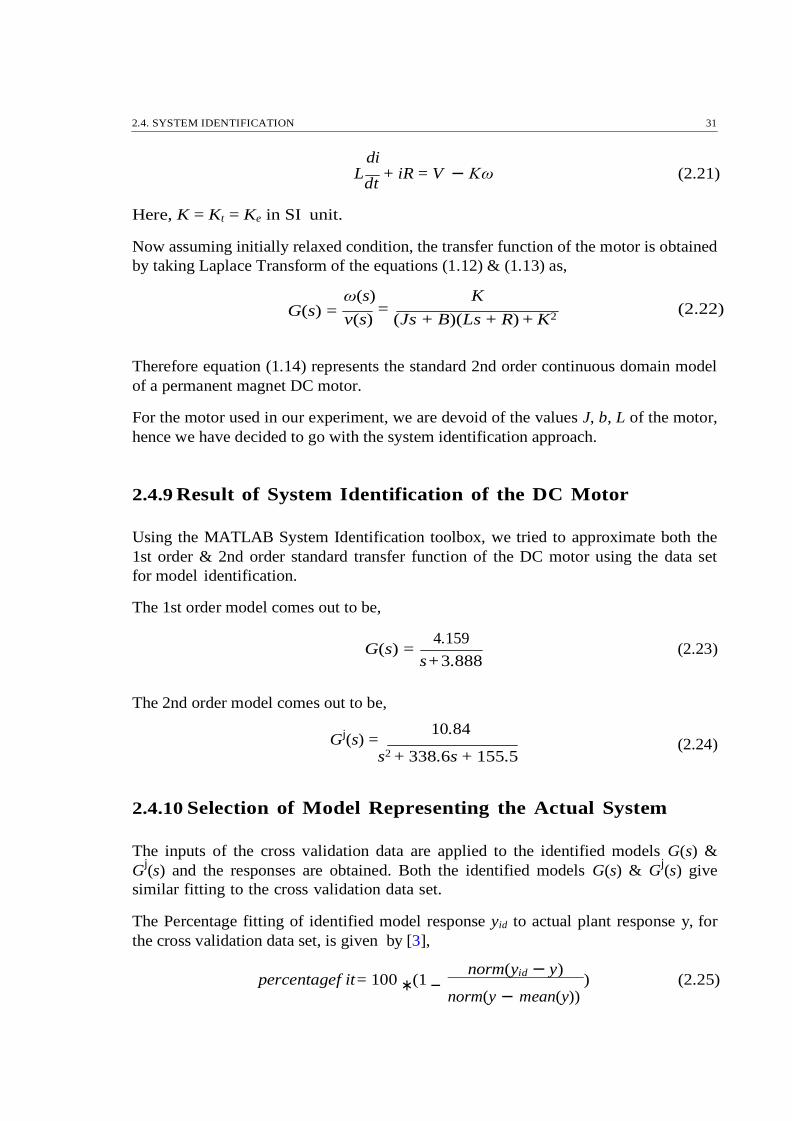
2.4. SYSTEM IDENTIFICATION 31
∗ −
di L
dt + iR = V − Kω (2.21)
Here, K = Kt = Ke in SI unit.
Now assuming initially relaxed condition, the transfer function of the motor is obtained
by taking Laplace Transform of the equations (1.12) & (1.13) as,
ω(s) K G(s) =
v(s) =
(Js + B)(Ls + R) + K2 (2.22)
Therefore equation (1.14) represents the standard 2nd order continuous domain model
of a permanent magnet DC motor.
For the motor used in our experiment, we are devoid of the values J, b, L of the motor,
hence we have decided to go with the system identification approach.
2.4.9 Result of System Identification of the DC Motor
Using the MATLAB System Identification toolbox, we tried to approximate both the
1st order & 2nd order standard transfer function of the DC motor using the data set
for model identification.
The 1st order model comes out to be,
G(s) =
4.159
s + 3.888
(2.23)
The 2nd order model comes out to be,
Gj(s) = 10.84
s2 + 338.6s + 155.5
(2.24)
2.4.10 Selection of Model Representing the Actual System
The inputs of the cross validation data are applied to the identified models G(s) &
Gj(s) and the responses are obtained. Both the identified models G(s) & G
j(s) give
similar fitting to the cross validation data set.
The Percentage fitting of identified model response yid to actual plant response y, for
the cross validation data set, is given by [3],
percentagef it = 100 (1 norm(yid − y)
) (2.25) norm(y − mean(y))

PLANT MODELING, CONTROLLER DESIGN AND THE PRACTICAL DC MOTOR SPEED CONTROL
SYSTEM 32
Now out of the two identified models G(s) & Gj(s), the model G(s) is selected as the
actual representation of the system based on the following criteria,
Both G(s) & G
j(s) provides similar fitting to the cross validation data, but the
order of G’(s) is more than G(s). Hence, from complexity point of view G(s) is
better representation of the DC motor plant.
Also if we observe the root locus plot, then one of the poles of Gj(s) lies very far
from the origin on s-plane. Hence, Gj(s) almost behaves like a first order system.
Figure 2.15: The Response of tt(s) to the Cross Validation Data
The percentage fitting given by G(s) to the cross validation data is 83.75 %.
Figure 2.16: Step Response of Identified Model tt(s)
Therefore, from the system identification experiment, we get the transfer function of
the DC motor as,
G(s) = 4.159
s + 3.888 (2.26)
•
•
2.5. SAMPLING TIME DECISION FOR DISCRETIZATION OF THE PLANT 33
The step response of the identified model is shown in figure2.16We can also represent
the transfer function of the DC motor as,
G(s) = 1.0697
τ s + 1
(2.27)
Where, τ = 0.2577 s, is the time constant of the system.
2.5 Sampling Time Decision For Discretization of
the Plant
Selection of proper sampling time is a matter of utmost importance for a discrete data
control system due to the following reasons,
• A very low sampling time leads to unnecessary computational overhead.
• To explain or understand observed phenomena
A very high sampling time may lead to loss of significant information about the
system dynamics.
A sufficiently high sampling time may lead to deterioration of performance &
even to instability in a discrete data control system.
Therefore we need to keep the points above in mind while discretizing the continuous
time transfer function & while implementing the closed loop system. Sampling time
should be such the chance of data loss is minimized at the same time leaving enough
time for the micro controller process the data within two sampling instants.
Usually selection of sampling time depends greatly on the measurement & instrumen-
tation system. In our experiment the speed encoder has a good resolution when the
sampling time is 20ms i.e the encoder can give an acceptable speed measurement at
a minimum interval of 20ms between two consecutive samples. Also, for execution
of a single statement, the Arduino micro controller requires a time of the order of
10−
6 second. Therefore, the selection of sampling time as Ts = 20ms leaves the micro
controller with enough time for processing of data and also does not lead to loss of
significant information. The DC motor identified transfer function has a time constant
of τ = 0.2577second which is almost 13 times of 20ms. Therefore we have selected
sampling time as 20ms for discretization of the transfer function of the DC motor as
well as for the discrete system design.
•
•

PLANT MODELING, CONTROLLER DESIGN AND THE PRACTICAL DC MOTOR SPEED CONTROL
SYSTEM 34
2.6 Discretization of the Closed Loop System
The functional block diagram of the closed loop system is shown below.
Figure 2.17: The functional block diagram of the basic embedded DC motor speed
control system with single micro controller board
For simplicity in realization of the control theory block diagram, from figure2.17, the
PWM generator block of the micro controller board is considered as the Zero Order
Hold Circuit (ZOH) block as it converts the digitally calculated duty ratio by the dicrete
controller into output DC analog PWM voltage and it holds a value of the duty ratio
until next sample comes. The comparator can simply be represented as a summer
block and the driver IC (actuator) along with the DC motor plant has been simply
represented as DC motor block. The encoder disc along with the speed optical encoder
and the pulse counter is considered as the sensor block. The sensor block output is the
reading of speed of the DC motor plant and hence the feedback loop is considered to
be unity feedback.
2.6.1 The Closed Loop Pulse Transfer Function
Here,
Gp(s) = Transfer Function of DC Motor Plant
Gh(s) = Transfer Function of ZOH circuit (D/A Converter)
G(s) = Gp(s) ∗ Gh(s)
G∗c (s) = Transfer Function of Discetre Controller
H(s) = Transfer Function of speed sensor = 1 (taken as unity)
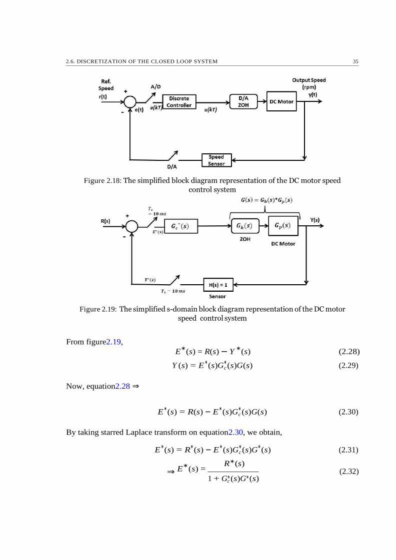
2.6. DISCRETIZATION OF THE CLOSED LOOP SYSTEM 35
Figure 2.18: The simplified block diagram representation of the DC motor speed
control system
Figure 2.19: The simplified s-domain block diagram representation of the DC motor
speed control system
From figure2.19,
Now, equation2.28 ⇒
E
∗(s) = R(s) − Y
∗(s) (2.28)
Y (s) = E∗(s)G
∗c (s)G(s) (2.29)
E∗(s) = R(s) − E∗
(s)G∗c (s)G(s) (2.30)
By taking starred Laplace transform on equation2.30, we obtain,
E∗(s) = R
∗(s) − E∗
(s)G∗c (s)G
∗(s) (2.31)
E∗
(s) = R∗(s)
1 + G∗c (s)G∗(s)
(2.32) ⇒

PLANT MODELING, CONTROLLER DESIGN AND THE PRACTICAL DC MOTOR SPEED CONTROL
SYSTEM 36
c
− Z
Now, taking starred Laplace transform on equation2.29 ⇒
Y
∗(s) = E
∗(s)G
∗c (s)G
∗(s) (2.33)
Using2.32
Y ∗
(s) = R∗(s)
1 + G∗c (s)G∗(s)
(s)G
∗c (s)G
∗(s) (2.34)
Y ∗(s) G
∗c (s)G
∗(s)
⇒ R∗(s)
= 1 + G∗(s)G∗(s)
(2.35)
The transfer function of the closed loop system is,
C∗(s) = Y
∗(s)
= G
∗c (s)G
∗(s)
(2.36)
R∗(s) 1 + G∗c (s)G∗(s)
Therefore, the pulse transfer function of the closed loop system is,
C(z) = Y (z)
= Gc(z)G(z)
(2.37)
R(z) 1 + Gc(z)G(z)
Here, 4.159
Gp(s) = s + 3.888
(2.38)
1 − e−sTs
Gh(s) = (2.39) s
Ts = sampling time = 20 ms
Therefore, G(s) = Gh(s) ∗ Gh(s) =
1 − e−sTs
s
4.159
(2.40) s + 3.888
Now, taking z transform, G(z) = (1 z
−1) [
4.159 ] (2.41)
s + 3.888
⇒ G(z) = (1 − z−1)Z[
1.0697 −
1.0697 ]
s s + 3.888
(2.42)

2.6. DISCRETIZATION OF THE CLOSED LOOP SYSTEM 37
c T 2
c
⇒ G(z) = (1 − z−1)[ 1.0697z
− 14.03z
] (2.43)
z − 1 0.0831
z − 0.92
⇒ G(z) = z − 0.92
(2.44)
2.6.2 Pulse Transfer Function of Dicrete PI Controller
The PI control action for analog controllers is given by [6],
1 u(t) = Kc[e(t) +
i
t
e(t)] (2.45) 0
Where,
u(t) = output of the controllers
e(t) = error input to the controllers
Kc = proportional gain of controllers
Ti = integral time or reset time of controllers
To obtain the pulse transfer function, we discretize equation2.45with integral term
approximated by trapezoidal summation. We get,
u(kT ) = K [e(kT ) + T
[ e(0) + e(T )
+ e(T ) + e(T )
+ ......... + e((k − 1)T ) + e(kT )
]]
Ti 2 2T
k
2 (2.46)
⇒ u(kT ) = K [e(kT ) + T
[Σ e((h − 1)T ) + e(hT )
]] (2.47)
Where,
T = sampling interval
We take, e((h − 1)T ) + e(hT )
= f (hT ), f (0) = 0 (2.48) 2
i h=1
i h=1
T
∫
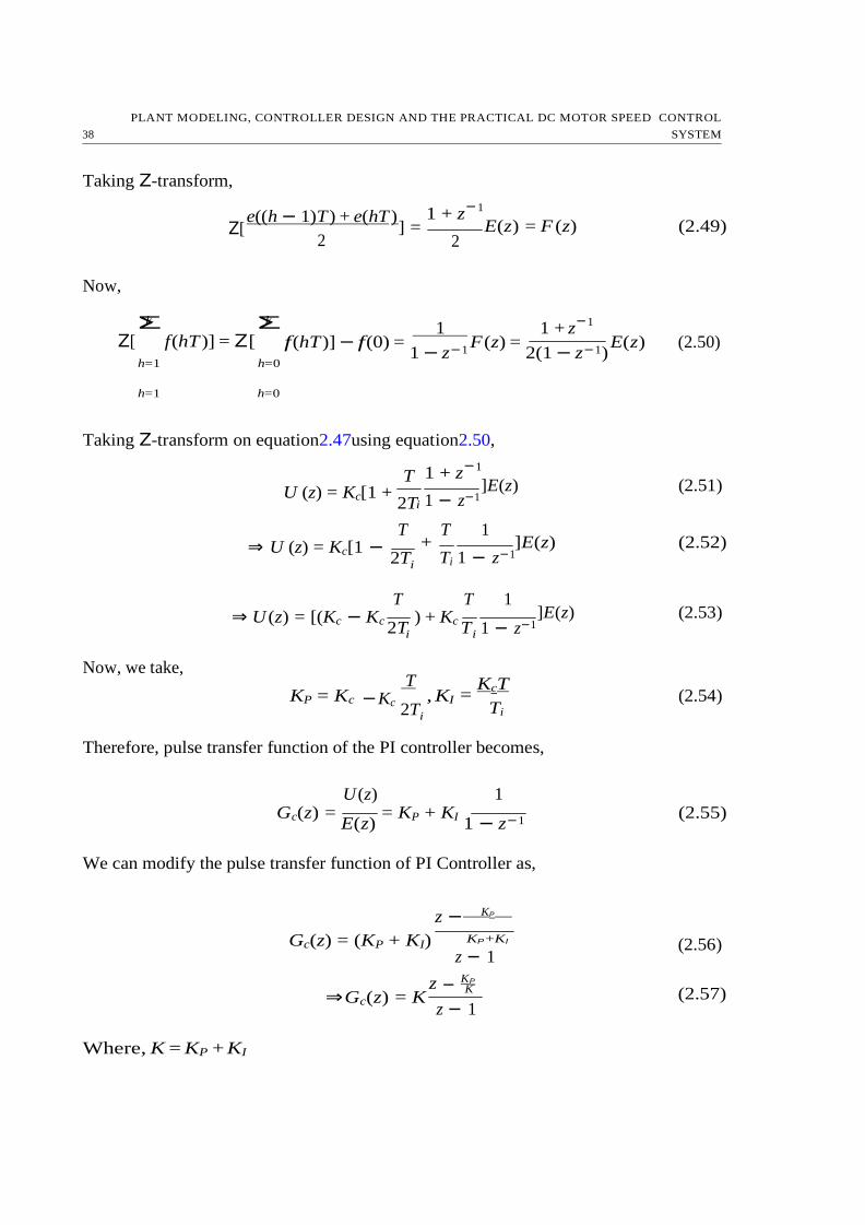
PLANT MODELING, CONTROLLER DESIGN AND THE PRACTICAL DC MOTOR SPEED CONTROL
SYSTEM 38
k
i
−
f (hT )] − f (0) = 1 − z−1
F (z) = 2(1 − z−1)
E(z) (2.50)
Taking Z-transform,
Z[
e((h − 1)T ) + e(hT )
] =
2
1 + z−1
E(z) = F (z) (2.49)
2
Now,
Σ Σ
1 1 + z−1
Taking Z-transform on equation2.47using equation2.50,
T U (z) = Kc[1 +
2T 1 + z
−1 ]E(z) (2.51)
1 − z−1
T ⇒ U (z) = Kc[1 −
2T
T 1 + ]E(z) (2.52)
Ti 1 − z−1
T T 1
⇒ U (z) = [(Kc − Kc 2T
) + Kc T
]E(z) (2.53) 1 − z−1
Now, we take, KP = Kc
T
− Kc 2T
, KI =
KcT
Ti
(2.54)
Therefore, pulse transfer function of the PI controller becomes,
U (z) 1 Gc(z) =
E(z) = KP + KI
1 − z−1 (2.55)
We can modify the pulse transfer function of PI Controller as,
z − KP
Gc(z) = (KP + KI) KP +KI
z − 1 (2.56)
Where, K = KP + KI
⇒ Gc(z) = K z KP
K (2.57) z − 1
h=0 h=1
h=0
f (hT )] = Z[
h=1
Z[
k
i
i
i
i

2.6. DISCRETIZATION OF THE CLOSED LOOP SYSTEM 39
2.6.3 Tuning of the Discrete PI Controller
The transfer function of the PI controller implemented is given as,
U (z) 1 Gc(z) =
E(z) = KP + KI
1 − z−1 (2.58)
2.6.3.1 Tuning Discrete PI Controller in MATLAB PID Tuner
Control System Toolbox of MATLAB has PID Tuner to perform automatic, interactive
tuning of PID controllers for plants represented by LTI models. We have used MATLAB
PID controller tuner for tuning of the discrete PI controller for the DC motor speed
control system. Configurable options availabble in the MATLAB PID Controller block
include:
• Controller type (PID, PI, PD, P, or I)
• Controller form (Parallel or Ideal)
• Time domain (continuous or discrete)
• Initial conditions and reset trigger
• Output saturation limits and built-in anti-windup mechanism
• Signal tracking for bumpless control transfer and multiloop control
Figure 2.20: The SIMULINK block diagram of the closed loop system used in
tuning
The default parallel form of PI controller is selected in the PID tuner for tuning pur-
pose.The Backward Euler approximation of the integrator part which uses the Back-
ward Rectangular (right-hand) approximation. An advantage of the Backward Euler
method is that discretizing a stable continuous-time system using this method always
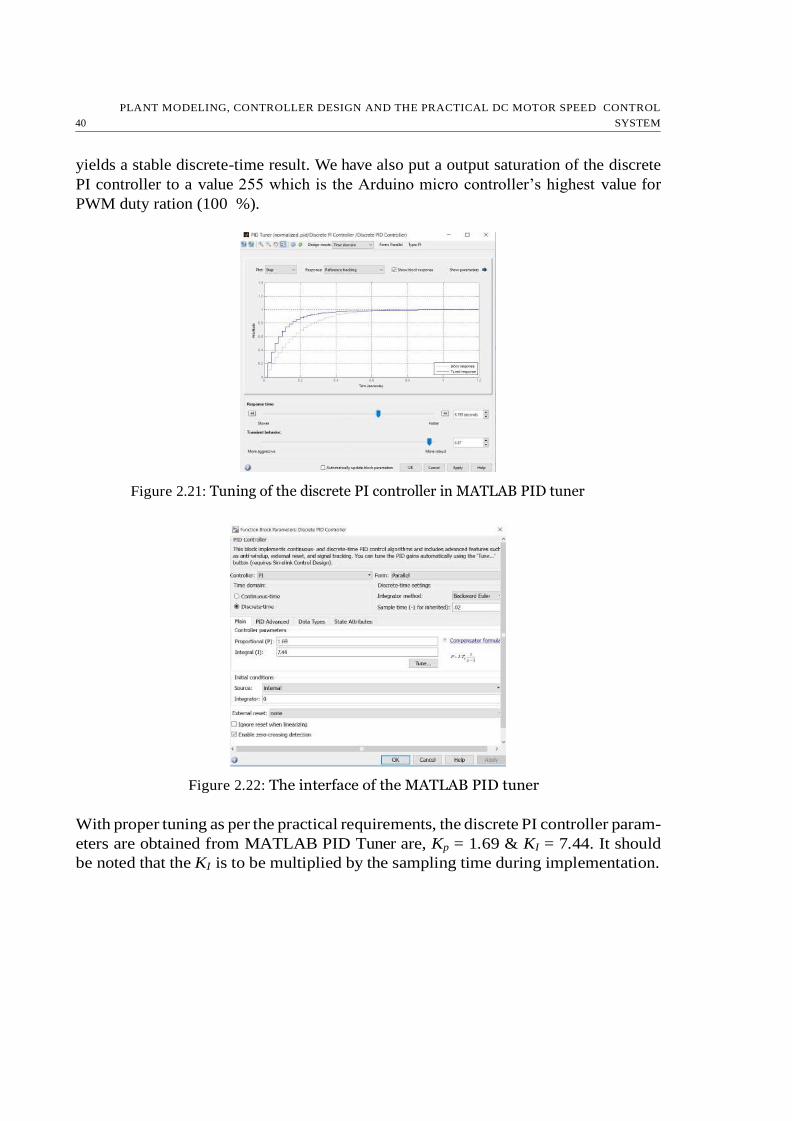
PLANT MODELING, CONTROLLER DESIGN AND THE PRACTICAL DC MOTOR SPEED CONTROL
SYSTEM 40
yields a stable discrete-time result. We have also put a output saturation of the discrete
PI controller to a value 255 which is the Arduino micro controller’s highest value for
PWM duty ration (100 %).
Figure 2.21: Tuning of the discrete PI controller in MATLAB PID tuner
Figure 2.22: The interface of the MATLAB PID tuner
With proper tuning as per the practical requirements, the discrete PI controller param-
eters are obtained from MATLAB PID Tuner are, Kp = 1.69 & KI = 7.44. It should
be noted that the KI is to be multiplied by the sampling time during implementation.

2.6. DISCRETIZATION OF THE CLOSED LOOP SYSTEM 41
K
2.6.3.2 Root Locus Design of Discrete PI Controller
From figure2.19, using equation2.57and2.44, the open loop transfer function of the
speed control system is,
Gc(z)G(z) = K z − KP
z − 1
.0831
z − 0.92
(2.59)
We locate the open loop poles of the DC motor control system in the z-plane as shown
in figure2.23below. Here, the location of open-loop zero of the PI controller need to
be determined.
Figure 2.23: The representation of closed loop system in z-domain
We take a dominant closed-loop pole at point P in the upper half of the z-plane.
The other design cosiderations in the design process are, damping coefficient, δ = 0.94
& ωd/ωs = 1/10 at point P .
The ratio ωd/ωs = 1/10 means that there are 10 samples per cycle of damped sinusoidal
frequency which ensures that there is no loss of significant information.
Now, for the closed loop system,
the magnitude of line joining origin & the point P ,
|z| = exp(− √ 2πδ ωd
) = 0.177 (2.60) 2 ω
the angle of the line at which point P is located is,
∠z = 2π ωd
ωs
= 36
◦ (2.61)
1 − δ s

PLANT MODELING, CONTROLLER DESIGN AND THE PRACTICAL DC MOTOR SPEED CONTROL
SYSTEM 42
Therefore, the location of closed loop pole at point P is,
z = |z|∠z = 0.177∠36◦ = 0.143 + j0.104 (2.62)
Using angle criterion, the angle deficiency for point P to be a closed loop pole is,
−173.5◦ − 173
◦ + 180◦ = −166.5
◦
The PI controller zero at z = KP /K must contribute an angle compensation of +166.5
◦
Therefore, by drawing the required angle compensation, from2.23, we get the PI
controller zero at z = 0.54 KP
= 0.54 (2.63) K
Now from equation2.59, using magnitude criterion,
K| z − 0.54 0.0831
|
= 1 (2.64)
z − 1 z − 0.92 z=0.143+j0.104
⇒ K = 19.83 (2.65)
Now, from equation2.63, KP = 10.7
Again, K = KP + KI =⇒ KI = 9.13
Therefore, z-domain representation of the designed discrete PI controller is given as,
U (z) 1 Gc(z) =
E(z) = 10.7 + 9.13
1 − z−1 (2.66)
Therefore, from the root locus design method, the PI controller parameters obtained
are KP = 10.7 and KI = 9.13
2.7 Practical Implementation of Discrete PI Con-
troller on µC
For practical implementation we have selected the PI controller parameters obtained
through tuning with the help of the MATLAB PID Tuner. This is because the simulated
response due to root locus designed PI controller is found to be aggressive (rise time
= 20 ms) and that of the MATLAB PID tuner designed PI controller is little less (rise

2.7. PRACTICAL IMPLEMENTATION OF DISCRETE PI CONTROLLER ON µC 43
ΣT
time = 180 ms) than the time constant of the DC motor plant (257.7 ms). Also the
settling time is quite larger in case of the root locus designed discrete PI controller.
Figure2.24below shows the simulated responses of the speed control system with
discrete PI controller designed by both root locus method and MATLAB PID Tuner.
Figure 2.24: Comparison of system responses with different design strategy for
discrete PI controller in SIMULINK
For practical implementation, the position algorithm of discrete PI controller is selected.
The position algorithm is shown below in equation2.67[6]. Here sampling time Ts =
0.02sec..
u(k) = KP
k
[e(k) + s e(k)] (2.67)
T i
k=1
Now, from the above equation,
K =
KP
I T
= 7.44 (2.68)
i
KP = 1.69 (2.69)
Therefore the representation of the implemented PI controller in discrete time domain
is, k−1 k
u(k) = KP e(k) + KI ∗ Ts Σ
e(k) = 1.69e(k) + 0.1488 Σ
e(k) (2.70)
The main theoretical problem with position algorithm of discrete PI controller is that
we need to store all the past error values. This problem is avoided on the Arduino µC
by defining an integer variable for the summation of error signal part. An integer in
the µC is of 32-bit size & can give a value as high as (232
− 1) which is sufficiently large
k=0 k=1

PLANT MODELING, CONTROLLER DESIGN AND THE PRACTICAL DC MOTOR SPEED CONTROL
SYSTEM 44
∗ ∗
enough to sum up all the past errors. The discrete PI controller algorithm implemented
in micro controller is shown below.
1: KP , KI, T (sampling time), integral threshold
2: integral sum = 0
3: error = setpoint - output
4: integral sum = integral sum + error
5: proportional = KP ∗ error
6: integral part = KI Ts integral sum
7: controller output = proportional + integral part
8: if (controller output > actuator maximum) then (controller output = actuator maximum
&& integral sum = integral threshold)
9: goto:step 3 if (setpoint available && output available)
The practical set up for implementation of DC motor speed control system is repre-
sented in figure2.25. Figure2.26, illustrates the response of the DC motor speed control
system in the wired setup with the discrete PI controller implemented in Arduino Due
board.
Figure 2.25: The practical setup for speed control of DC motor (wired fashion)
Figure2.27, illustrates the response of the DC motor speed control system in the wired
setup with the discrete PI controller implemented in Arduino Uno board.

2.7. PRACTICAL IMPLEMENTATION OF DISCRETE PI CONTROLLER ON µC 45
Figure 2.26: Wave forms of the wired speed control setup with discrete PI controller
(with Arduino Due board)
Figure 2.27: Wave forms of the wired speed control setup with discrete PI controller
(with Arduino Uno board)
There are some jitters in the response of the practical closed loop system and the
reasons to this may be as follows,
The encoder disc attached to the shaft of the DC motor has 20 slots and for 20
ms sampling the resolution is 2.5 rps value. Hence speed encoder reading may
fluctuate some times.
The control input calculated by the discrete PI logic is quantized into an 8 bit
number discarding the floating point numbers. This is because in Arduino em-
bedded environment, PWM duty ratio is an 8 bit number (0-255) in discrete steps
of 1.
• The resolution of PWM duty ratio of Arduino board is (100/255)% = 0.392%.
•
•

46 REFERENCES
Also from figure2.26and2.27, it is clear that Arduino Due performs better speed con-
trol due to its better numerical computational capability and quantization capability.
2.8 Chapter Summary
In this chapter we have discussed brief introduction to the DC motor speed control
method adopted. Then components and devices used for practical set up has been
discussed. Modeling of the DC motor plant using System Identification procedure has
been performed and the transfer function of the plant has been obtained. Then we have
tried discrete PI controller design based on the model of DC motor obtained from sys-
tem identification using both Root Locus method and MATLAB PID tuner. MATLAB
PID Tuner tuned PI controller is seen to be performing better in simulation and hence
adopted for implementation in hardware. Then discrete PI algorithm implemented in
micro controller has been given. Then we observed the response of the speed control
system with the discrete PI controller implemented in Arduino embedded environment.
References
[1] Ljung, L., 1999. System Identification: Theory for the User, PTR Prentice Hall
Information and System Sciences Series.
[2]Salah, M.S., 2009. Parameters identification of a permanent magnet DC motor
(Doctoral dissertation, The Islamic University of Gaza).
[3] Roy, P., Borah, M., Majhi, L. and Singh, N., 2015, September. Design and Imple-
mentation of FOPID Controllers by PSO, GSA and PSOGSA for MagLev System.
In Advanced Computing and Communication (ISACC), 2015 International Sympo-
sium on (pp. 10-15). IEEE.
[4] DC Motor Speed: System Modeling - Control Tutorials
ctms.engin.umich.edu
[5] Dubey, G.K., 2002. Fundamentals of electrical drives. CRC Press
[6] Ogata, K., 1995. Discrete-time control systems (Vol. 2). Englewood Cliffs, NJ: Pren-
tice Hall. Vancouver

Chapter 3
Bluetooth Technology & The
Wireless Networked Control System
3.1 Introduction
Bluetooth is the most popular personal-area network (PAN) system [2]. A personal-
area network (PAN) is a very small wireless network that is created informally or on an
ad hoc basis [2]. Bluetooth industry standard started developing from the late winter
of 1998 when Ericsson, IBM, Intel, Nokia, and Toshiba formed the Bluetooth Special
Industry Group (SIG) to develop and promote a global solution for short range wireless
communication [3]. The IEEE standardized Bluetooth as IEEE 802.15.1, but standard
is no longer maintained by IEEE [4]. The Bluetooth SIG supervises the development of
the specification and manages the qualification program, and protects the trademarks
[4].
The primary aim of Bluetooth wireless technology is to serve as the universal low cost,
user friendly, wireless interface replaces the variety of proprietary cables that need to
be carried to connect personal devices such as notebook computers, cellular phones,
personal digital assistants (PDAs), digital cameras etc. [3]. Personal devices usually
employ RS-232 serial port protocol. Therefore, It impossible to use the same set of
cables to interconnect devices from different manufactures, and sometimes even from
the same manufacturer due to need various types of proprietary connectors and pin
arrangements [3]. Bluetooth provides replacement for cables to interconnect, and also
to form ad hoc network between various personal devices.
47

48 BLUETOOTH TECHNOLOGY & THE WIRELESS NETWORKED CONTROL SYSTEM
Figure 3.1: The Bluetooth Technology Logo
3.2 General Communication Network Architecture
The protocols & components required to satisfy application requirements are defined
by architecture of a network [6]. Open System Interconnect (OSI) is a seven-layer
reference model for explaining the architecture of a network [6]. OSI is developed by
International Standards Organization (ISO). Complete set of network functions are
specified by OSI and the OSI reference model is a instrumental model for depicting
various standards and interoperability of a wireless network [6].
The different OSI layers and their network functionality are explained below as per [6]:
Application layer (layer 7): Communications among users are established by
this layer and the layer also gives basic communication services such as file transfer
and e-mail. Examples of application of this layer are: Simple Mail Transfer
Protocol (SMTP), HyperText Transfer Protocol (HTTP), File Transfer Protocol
(FTP).
Presentation layer (layer 6): This layer does negotiation of data transfer
syntax for the application layer and translations between different data formats
depending upon necessity.
Session layer (layer 5): Sessions between applications are established, managed
and terminated by this layer. In wireless networks, wireless middleware and access
controllers provide this type of connectivity.
Transport layer (layer 4): Mechanisms for establishment, maintenance, and
orderly terminations of virtual circuits are provided by this layer, while the higher
layers are shielded from the network implementation details. Virtual circuits are
connections between network applications from one end of the communications
circuit to another 9for example; between web browser on a PC to a server).
Transmission Control Protocol (TCP) operates at this layer.
•
•
•
•

3.2. GENERAL COMMUNICATION NETWORK ARCHITECTURE 49
Figure 3.2: OSI Refernce Model Layers [6]
Network layer (layer 3): This layer does routing data packets through the
network from source to destination. This routing is done for ensuring that the
data packets are sent in a direction leading to the destination. Protocols such as
Internet Protocol (IP) operate at this layer.
Data link layer (layer 2): This layer tries to ensure medium access, syn-
chronization and error control between two entities. In case of wireless network,
this layer is responsible for the coordination of access to the air medium and
minimization of propagation error. Most of the wireless networks have a com-
mon technique for performing data link layer operations which is independent of
actual way of transmission.
Physical layer (layer 1): Actual transmission of information through the
medium is provided by this layer. Radio waves and infrared light are included in
this layer.
The combination of the different layers of OSI network architecture depicts the func-
tionality of a wireless network. It is important to notice that wireless networks directly
implement only the lower layers of the architecture [6]. it is seen that a wireless Network
Interface Card (NIC) implements only the data link layer and physical layer functions.
Each layer of the OSI architecture provides support to the layers above it. Figure3.2
shows that each OSI model layer communicate across the network to the respective
layer of the peer. But, the actual data transmission takes place only at physical layer.
Therefore, in this layering process, a particular layer puts its protocol information into
frames which are place within frames of lower layers [6]. The frame sent by the physical
•
•
•

50 BLUETOOTH TECHNOLOGY & THE WIRELESS NETWORKED CONTROL SYSTEM
layer includes frames from all higher layers. At the destination, each layer sends the
respective frames to the higher layers to ease the protocol between peer layers.
3.3 The Bluetooth Radio
Bluetooth is a digital radio standard that operates globally in the unlicensed 2.4 GHz
ISM (Industrial, Scientific and Medical) short-distance radio frequency band [2,4].
Blutooth employs a radio technology called frequency-hopping spread spectrum (FHSS)
[2,4]. Bluetooth operates over 79 channels with a frequency band 2.402-2.480 GHz in
most of the countries and over 23 channels with frequency a band 2.44652.4835 GHz in
very few countries [2,7].Each of the 79 or 23 channels has a bandwidth of 1 M Hz [5].
The hop rate is 1600 hops/second and the dwell time on each frequency is 1/1600 =
625 µs [2]. Bluetooth divides transmitted data into packets, and transmits each packet
on one of 79 or 23 designated Bluetooth channels [4]. There are also guard bands 2
M Hz wide at the bottom end and 3.5 M Hz wide at the top to prevent interference
[4,7].
Figure 3.3: Functional Blocks in a Bluetooth System [7]
Since Bluetooth is a radio frequency communications technology, Bluetooth devices do
not have to be in visual line of sight of each other [4]. Range of a Bluetooth device is
power dependent and the effective range varies with application [4]. There are various
classes of Bluetooth radios and their power range along with the range have been
provided in Table3.1.
Class Max. Permitted Power (mW) Max. Permitted Power (dBm) Range (m)
1 100 20 100
2 2.5 4 10
3 1 0 1
Table 3.1: Different Classes of Bluetooth Radio [4]

3.4. BLUETOOTH AS WPAN 51
3.4 Bluetooth as WPAN
A WPAN (Wireless Personal Area Network) is a wireless network for interconnecting
devices centered around an individual person’s workspace. Bluetooth PAN (Personal
Area Network) is used for close-quarters connections between Bluetooth compatible
devices such as PCs, laptops, mobile phones, PDAs. In earlier days, special-purpose
proprietary cables have been used for interconnection of personal devices [7]. But
user experience with these cables are not convenient as they are prone to damage,
loss and aslo they bulky, messy to carry. So in order to adress these issues, WPAN
technology has evolved. The Bluetooth WPAN technology utilizes a short-range radio
communication link optimized for low power, battery operated, light weight and small
personal devices [7]. It is created in a ad hoc or temporary manner whenever required.
3.4.1 General Requirements of a WPAN
There are various requirements for a WPAN to be accepted widely by people as well
as industry and they are as follows [7]
The WPAN technology should not effect the personal device’s weight, power
consumption, form factor, cost, convenience of use or other characteristics in a
significant way.
The WPAN technology should fulfill the design and marketing requirements of
not only the consumer market but also the business market.
Users should be able to use the WPAN connectivity to connect the personal
device around their vicinity without data services or ethernet connectivity.
Communicating devices under a WPAN should remain connected without line
of sight of each other. This standard leads to use of radio frequency (RF) tech-
nologies in WPAN technology and Bluetooth is one of the RF communication
technology.
3.4.2 Difference of WPAN from WLAN
Fundamentally, WPAN differs from Wireless Local Area Network (WLAN) in three
ways [7]:
Power Levels and Coverage: WLAN technology is intended and often opti-
mized for larger coverage. Therefore, the power consumption of the devices for
•
•
•
•
•

52 BLUETOOTH TECHNOLOGY & THE WIRELESS NETWORKED CONTROL SYSTEM
covering larger distances increases. WLAN devices are usually connected to a
power plug or they use the wireless network for a relatively short time when un-
plugged. Therefore, WLAN is usually said to connect ”portable” devices which
are moved less frequently, powered from wall sockets and have relatively longer
periods of connections
On the other hand, WPAN technology trades off coverage for lower power con-
sumption. Therefore, WPAN is said to be oriented towards ”mobile” personal
devices which operate on batteries and have relatively lower periods of connection.
Control of the Medium: WPAN implements a controlling mechanism that reg-
ulates the data transmissions of the devices connected to the network in order to
provide required bandwidth guarantees for various connections. A typical WPAN
device does not require to have a network-observable and network-controllable
state. WPAN is ad hoc in nature i.e. a master must be present for communica-
tions to occur.
On the other hand, WLAN does not usually employ controlling mechanism for
regulating data transmissions of the devices as it may not be always desirable
considering the large distance covered. Primary objective of WLAN is to provide
the data services infrastructure typically available through a LAN to the client
devices. Once a client device joins the WLAN network, the device typically
remains connected to the WLAN until the device moves away from the network’s
boundaries. A typical WLAN device require to have a network-observable and
network-controllable state being part of a larger infrastructure.
Life Span of Network: WLAN’s existence is independent of the constituent
devices. Therefore, they are said to be existed uninterrupted. On the other hand,
WPAN exists only when master device participates and the network no longer
exists when the master does not participate. So the lifespan of WPAN is finite.
3.5 The Bluetooth Protocol Stack
The protocol stack of a communication network is nothing but hardware or software
realization of the standard protocols which enables the connected devices to commu-
nicate with each other [1]. There are certain layers in the protocol stack with different
applications.
The lowest layer of the Bluetooth protcol stack is the physical radio, which acts as the
radio front and also depicts the attributes of the permissible power levels, channel ar-
rangements, frequency bands and radio receiver’s susceptivity [1]. The baseband layer
looks after Bluetooth’s physical and media access control. The devices to be paired
share various control messages for managing and configuring the baseband configura-
tions [1].
•
•

3.5. THE BLUETOOTH PROTOCOL STACK 53
Figure 3.4: The Bluetooth Protocl Stack & Its Mapping with OSI ISO Reference
Model[5,7]
The Link manager layer looks after the processing related to link manager protocol [1].
There are two different types of links exist in Bluetooth : Asynchronous Connection
Links ACLs and Synchronous Connection-oriented Links SCOs [5]. An SCO link en-
sures guaranteed delay and bandwidth apart from the possible interruption caused by
high priority link manager protocol messages [5]. SCO links are suitable for average
quality music and voice transmission [5]. A slave can have three SCO links with the
same master at max, or two SCO links with different masters at most and a master
can have up to three SCO links with three different slaves at most [5]. ACLs are useful
for non-real time traffic. Only a single ACL link can be there between a given master
and a slave [5].
The control layer or the Host Controller Interface layer defines a standard interface
or independent way of communication with the Bluetooth module [1]. The L2CAP
(Logical Link Control Adaptation Protocol ) layer provides services to the upper levels
off the connection and with the connection on [5]. The functions of L2CAP layer are
as follows [5]
• Protocol Multiplexing.
Segmentation and reassembly of the protocol data units that comes from upper
layers.
• Quality of service (QoS) support.
•

54 BLUETOOTH TECHNOLOGY & THE WIRELESS NETWORKED CONTROL SYSTEM
Internet Protocol (IP) can be directly implemented in L2CAP layer. But, it is usually
implemented in PPP (Point-to-Point Protocol ) layer above RFCOMM [5]. RFCOMM
layer mainly does emulation of serial communication port [1]. Due to RFCOMM layer,
Bluetooth chip or module can be easily connected to PC or other such devices using
USB or UART protocols [1]. SDP (Service Discovery Protocol ) layer enables a Blue-
tooth slave device to find services and its peers [1]. TCS layer is basically provides
telephony control specifications.
3.5.1 Security in Bluetooth Protocol
Bluetooth protocol has certain security measures which are explained here as per [5].
Bluetooth protocol security can be divided into three modes as follows:
• 1st Mode: Nonsecure.
• 2nd Mode Service level enforced security (after establishment of channel).
• 3rd Mode Link level enforced security (before establishment of channel).
Link level authentication and encryption are handled with the help of basic four entities:
• 48-bit unique Bluetooth device address assigned to each device.
• A random private authentication key.
• A random private encryption key.
A 128-bit random number dynamically generated by each Bluetooth device. This
number changes frequently.
In Bluetooth protocol, there are two security levels
• Trusted.
• Untrusted
There are also three security levels defined for services:
• Open services.
• Services with authentication requirement.
• Services with authentication and authorization requirements.
•
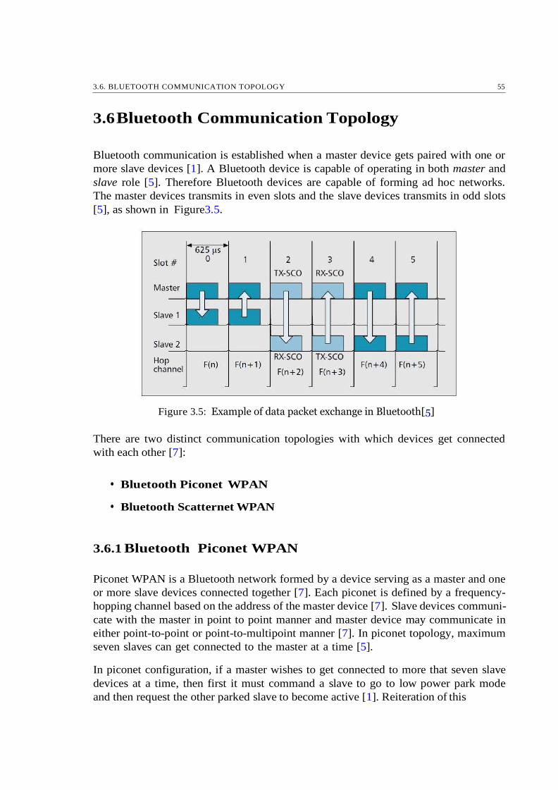
3.6. BLUETOOTH COMMUNICATION TOPOLOGY 55
3.6 Bluetooth Communication Topology
Bluetooth communication is established when a master device gets paired with one or
more slave devices [1]. A Bluetooth device is capable of operating in both master and
slave role [5]. Therefore Bluetooth devices are capable of forming ad hoc networks.
The master devices transmits in even slots and the slave devices transmits in odd slots
[5], as shown in Figure3.5.
Figure 3.5: Example of data packet exchange in Bluetooth[5]
There are two distinct communication topologies with which devices get connected
with each other [7]:
• Bluetooth Piconet WPAN
• Bluetooth Scatternet WPAN
3.6.1 Bluetooth Piconet WPAN
Piconet WPAN is a Bluetooth network formed by a device serving as a master and one
or more slave devices connected together [7]. Each piconet is defined by a frequency-
hopping channel based on the address of the master device [7]. Slave devices communi-
cate with the master in point to point manner and master device may communicate in
either point-to-point or point-to-multipoint manner [7]. In piconet topology, maximum
seven slaves can get connected to the master at a time [5].
In piconet configuration, if a master wishes to get connected to more that seven slave
devices at a time, then first it must command a slave to go to low power park mode
and then request the other parked slave to become active [1]. Reiteration of this

56 BLUETOOTH TECHNOLOGY & THE WIRELESS NETWORKED CONTROL SYSTEM
Figure 3.6: The Bluetooth Piconet Topology[5]
procedure allows the master to get paired with more than seven slaves. The master
device determines allocation of bandwidth and mode of communication among the
slaves [1].
3.6.2 Bluetooth Scatternet WPAN
Bluetooth scatternet topology enables us to create multihop WPAN [5]. A multihop
network is one where two nodes can communicate with each other with the help of other
nodes as relays, without direct connection between them [5]. In scatternet configura-
tion, a number of operational Bluetooth piconets overlap in time and space through
common nodes [7]. A node in scatternet topology can be master in only one of the
piconets, but can be a slave in several piconets [5,7].
Figure 3.7: The Bluetooth Scatternet Topology[5]

3.7. STATES OF A BLUETOOTH DEVICE 57
Bridge nodes in overlapping areas of a scatternet network involves with members of
different piconets on time sharing basis [1]. Interference between different piconets is
not seen as they operate with different frequency hopping sequence [1].
3.7 States of a Bluetooth Device
After Bluetooth connection is established, a Bluetooth device can be at any one state
among total eight states [1]. The eight states are explained below [1]:
Standby State: When the Bluetooth device is powered on and it has not estab-
lished any connection to other devices.
Inquiry State: It is the state where a device sends request to discover devices
around its coverage zone to pair up.
Page Mode: Paging is the process of forming a connection between two Blue-
tooth devices. Before this connection can be initiated, each device needs to know
the address of the other.
Connected State: In connected state, a device establishes Bluetooth link with
one or more other devices and to do this, the device requires an active address.
Transmit State: A slave device is said to be in transmit state when it transmits
data to master device.
Sniff State: In sniff state a slave is said to be connected to piconet network
virtually with a reduced duty cycle.
Park State: A device in park state surrenders its active address and does not
transmit data even if it is linked to the piconet network.
Hold State: Hold mode is a temporary, power-saving mode where a device sleeps
for a defined period and then returns back to active mode when that interval has
passed. The master can command a slave device to hold.
3.8 Different Versions of Bluetooth
Since the inception of Bluetooth, different versions have been evolved. Various versions
of Bluetooth are explained below [4]:
•
•
•
•
•
•
•
•

58 BLUETOOTH TECHNOLOGY & THE WIRELESS NETWORKED CONTROL SYSTEM
Figure 3.8: Different States of a Bluetooth Device[1]
Bluetooth 1.0 and 1.0B: They are the earlier most versions of Bluetooth.
Their connecting process involved mandatory hardware device transmission mak-
ing anonymity impossible at the protocol level. This was a major setback for some
certain services planned for Bluetooth communications. These devices also had
problems with interoperability.
Bluetooth 1.1: This version was ratified as IEEE Standard 802.15.1-2002.
Many faults found in version 1.0B were fixed in this version. Possibility of non-
encrypted channel and Received Signal Strength Indicator (RSSI) were also in-
corporated in this version of Bluetooth.
Bluetooth 1.2: Major improvement in this version were faster connection and
discovery. Adaptive Frequency-Hopping spread spectrum (AFH) has been intro-
duced in this version, which improves resistance to radio frequency interference by
avoiding the use of crowded frequencies in the hopping sequence. Extended Syn-
chronous Connections (eSCO) have been introduced, which uplift voice quality of
audio links by allowing retransmissions of corrupted packets, and may optionally
increase audio latency to provide better concurrent data transfer. This version
was retified as Ratified as IEEE Standard 802.15.12005.
Bluetooth 2.0 + EDR : This version introduced Enhanced Data Rate (EDR)
for faster data transfer. Although EDR is an optional feature. Apart from EDR,
there other minor improvements are there in this version.
Bluetooth 2.1 + EDR: This version was adopted by Bluetooth SIG in 2007.
The key feature os this version is Secure Simple Paring. Other improvements
include Extended Inquiry Response, which gives more information during
inquiry procedure to enable better filtering of devices before connection.
Bluetooth 3.0 + HS: The main feature of this version is Alternative MAC/-
PHY (AMP) which enables the use of alternative MAC and PHYs to transport
•
•
•
•
•
•

3.8. DIFFERENT VERSIONS OF BLUETOOTH 59
Bluetooth profile data. This allows bluetooth to be in low power mode when in
idle and to use faster radio when large data need to be sent. Enhanced power
control feature was incorporated in this version.
Bluetooth 4.0 + LE: It was incorporated in 2010 and called as Bluetooth Smart.
This version includes Classic Bluetooth, Bluetooth high speed and Bluetooth low
energy protocols. Bluetooth high speed is based on Wi-Fi, and Classic Bluetooth
consists of legacy Bluetooth protocol.
Bluetooth 4.1 : Formal introduction of Bluetooth 4.1 took place in 2013. This
specification is an incremental software update to Bluetooth Specification v4.0,
and not a hardware update. The update incorporates Bluetooth Core Specifica-
tion Addenda (CSA 1, 2, 3 4) and adds new features that improve consumer
usability.New features include increased co-existence support for LTE, bulk data
exchange ratesand aid developer innovation by allowing devices to support multi-
ple roles simultaneously. The other important new features included are Low Duty
Cycle Directed Advertising, L2CAP Connection Oriented and Dedicated Channels
with Credit Based Flow Control, Dual Mode and Topology, Limited Discovery
Time etc.
Bluetooth 4.2: It was introduced in 2014. This version introduced features for
Internet of Things. Other major improvements are as folows:
– Low Energy Secure Connection with Data Packet Length Extension.
– Link Layer Privacy with Extended Scanner Filter Policies
– Internet Protocol Support Profile (IPSP) version 6 ready for Bluetooth
Smart things to support connected home.
Bluetooth 5: Bluetooth 5 was unveiled in June, 2016. The feature of this
version is mailny focused on emerging Internet of Things technology. It also
has quadruple the range, double the speed, and provides an eight-fold increase
in data broadcasting capacity of low energy Bluetooth transmissions compared
to Bluetooth 4.x versions, which could be important for IoT applications where
nodes are connected throughout a whole house. It is important to note that park
state was removed in this version. The major improvements of this version are
as follows:
– Slot Availability Mask (SAM).
– 2 Mbit/s PHY for LE.
– LE Long Range.
– High Duty Cycle Non-Connectable Advertising.
– LE Advertising Extensions.
•
•
•
•

60 BLUETOOTH TECHNOLOGY & THE WIRELESS NETWORKED CONTROL SYSTEM
Bluetooth Version Data Rate Range (m)
1.2 721 kbit/s 10
2.x 2.1 Mbit/s 10
3.0 25 Mbit/s 10
4.x 25 Mbit/s 60
5 50 Mbit/s 100
Table 3.2: Different Versions of Bluetooth with Their Speed and Range [4]
3.9 HC-05 Bluetooth Module
Bluetooth module is a device where Bluetooth wireless facility is embedded as replace-
ment of serial cables and which can be interfaced with any computer or any other com-
puting device [1]. Bluetooth modules use UART (Universal Asynchronous Receiver/-
Transmitter) protocol for serial communication. They have one pin for transmission
(TX) and another pin (RX) for receiving serial data. Therefore Bluetooth communica-
tion is bidirectional or duplex in nature. Different types of Bluetooth modules available
in the market are [1]:
1. Industrial Level : HC-03, HC-04
2.Civil Level : HC-05, HC-06
The modules with even number (e.g. HC-04) comes with a default master or slave
configuration which can’t be changed later [1]. On the other hand modules with odd
number (e.g. HC-05) can be configured to act as both master & slave mode by using
appropriate AT commands [1].
3.9.1 Connection of HC-05 with Arduino Board
The HC-05 module has both transmitter pin (TXD) and receiver pin (RXD) which are
used to obtain data from the Arduino board for wireless transmission and to send wire-
lessly transmitted data to the Arduino board as per UART (Universal Asynchronous
Receiver/Transmitter) protocol. Arduino Due board has four pairs of receiver and
transmitter pins(TX0-RX0, TX1-RX1, TX2-RX2, TX3-RX3) whereas Arduino Uno
board has only single pair of receiver and transmitter pins (TX-RX). The receiver
pin of Arduino board needs to be connected to the transmitter pin of HC-05 mod-
ule and the transmitter pin of Arduino board needs to be connected to the receiver
pin of HC-05 module, for e.g. TX3 pin with RXD and RX3 pin with TXD. Power
supply to the HC-05 module is given (at VCC pin) from the 5V or 3.3 V pin of the
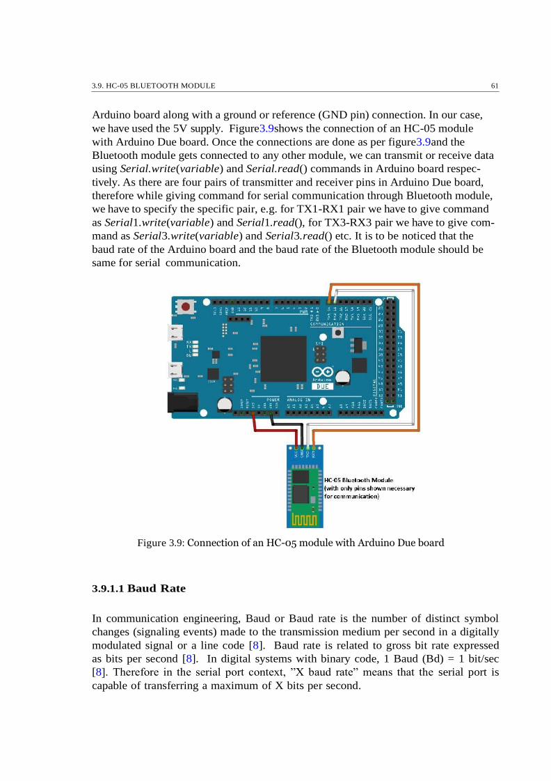
3.9. HC-05 BLUETOOTH MODULE 61
Arduino board along with a ground or reference (GND pin) connection. In our case,
we have used the 5V supply. Figure3.9shows the connection of an HC-05 module
with Arduino Due board. Once the connections are done as per figure3.9and the
Bluetooth module gets connected to any other module, we can transmit or receive data
using Serial.write(variable) and Serial.read() commands in Arduino board respec-
tively. As there are four pairs of transmitter and receiver pins in Arduino Due board,
therefore while giving command for serial communication through Bluetooth module,
we have to specify the specific pair, e.g. for TX1-RX1 pair we have to give command
as Serial1.write(variable) and Serial1.read(), for TX3-RX3 pair we have to give com-
mand as Serial3.write(variable) and Serial3.read() etc. It is to be noticed that the
baud rate of the Arduino board and the baud rate of the Bluetooth module should be
same for serial communication.
Figure 3.9: Connection of an HC-05 module with Arduino Due board
3.9.1.1 Baud Rate
In communication engineering, Baud or Baud rate is the number of distinct symbol
changes (signaling events) made to the transmission medium per second in a digitally
modulated signal or a line code [8]. Baud rate is related to gross bit rate expressed
as bits per second [8]. In digital systems with binary code, 1 Baud (Bd) = 1 bit/sec
[8]. Therefore in the serial port context, ”X baud rate” means that the serial port is
capable of transferring a maximum of X bits per second.

62 BLUETOOTH TECHNOLOGY & THE WIRELESS NETWORKED CONTROL SYSTEM
3.9.1.2 Software Serial Transmitter and Receiver in Arduino Board
Any two digital I/O pin of an Arduino board can be configured as a pair of se-
rial transmitter and receiver pins by using a default software serial library avail-
able in Arduino IDE software. Software serial configuration is needed when we want
serial communication for an Arduino board with all the serial transmitter and re-
ceiver hardware pins engaged. The software serial library is imported with the code
#include < Sof twareSerial.h > followed by Sof twareSerial BT serial(Rx, T x);
(Where BT serial is the name given to the software defined serial communication port
and Rx, T x are the numbers of the digital pins to be used as receiver and transmitter
respectively). In this case the baud rate for serial communication is defined with the
code BT serial.begin(baud rate).
Use of sofware serial port is mainly needed in case of Arduino Uno board as it has single
dedicated serial communication port. If we connect the Arduino Uno board to the PC
via USB cable for data acquisition while Bluetooth module connected to the TX-RX
pins, then proper data acquisition is not possible. This is because serial communication
with the PC and the Bluetooth module uses the same dedicated hardware. Hence
to perform both data acquisition and Bluetooth communication simultaneously using
Arduino Uno, we can use software defined serial communication port for connecting
the Bluetooth module.
Figure 3.10: Connection of an HC-05 module with Arduino Uno board
3.9.2 Configuration of HC-05 Using AT Commands
HC-05 Bluetooth module can be configured using AT commands by connecting it to
an Arduino board connected to a PC via USB cable. The steps necessary to drive an

3.9. HC-05 BLUETOOTH MODULE 63
HC-05 module to AT command mode are given below,
TX pin of Arduino should be connected to TXD pin of HC-05 and RX pin of
Arduino should be connected to RXD pin of HC-05.
• Arduino board should be connected to the PC via USB cable.
A blank sketch, as shown in figure3.11, should be uploaded to the Arduino board
from Arduino IDE software.
5V power supply should be given to the enable (EN) pin of HC-05 from the
Arduino board (with the ground connected).
The reset button of the HC-05 module is pressed. The button should be kept
pressed.
The 5v power supply should be provided at the VCC pin of HC-05 from arduino
board.
The HC-05 module goes to AT command mode and the reset button should be
released.
Arduino IDE console should be opened up and the baud rate of the console should
be set to 38400.
Figure 3.11: Blank sketch uploaded to Arduino board
•
•
•
•
•
•
•

64 BLUETOOTH TECHNOLOGY & THE WIRELESS NETWORKED CONTROL SYSTEM
Once HC-05 module goes to AT command mode, we can send AT commands to it
from the Arduino IDE console. There are many types of AT commands for the HC-05
Bluetooth. We are going to highlight the commands that we have used for our purpose
in table3.3below.
Table 3.3: Different AT commands used for HC-05 module
Figure 3.12: Different pins of HC-05 module
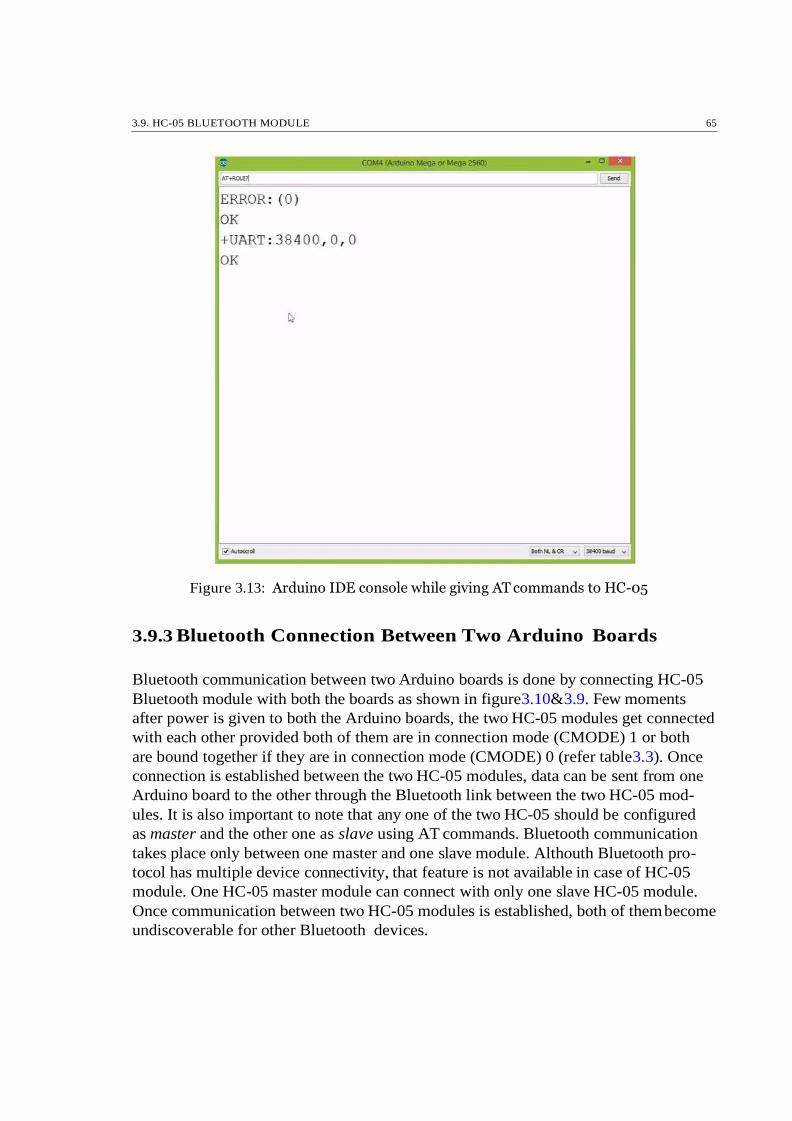
3.9. HC-05 BLUETOOTH MODULE 65
Figure 3.13: Arduino IDE console while giving AT commands to HC-05
3.9.3 Bluetooth Connection Between Two Arduino Boards
Bluetooth communication between two Arduino boards is done by connecting HC-05
Bluetooth module with both the boards as shown in figure3.10&3.9. Few moments
after power is given to both the Arduino boards, the two HC-05 modules get connected
with each other provided both of them are in connection mode (CMODE) 1 or both
are bound together if they are in connection mode (CMODE) 0 (refer table3.3). Once
connection is established between the two HC-05 modules, data can be sent from one
Arduino board to the other through the Bluetooth link between the two HC-05 mod-
ules. It is also important to note that any one of the two HC-05 should be configured
as master and the other one as slave using AT commands. Bluetooth communication
takes place only between one master and one slave module. Althouth Bluetooth pro-
tocol has multiple device connectivity, that feature is not available in case of HC-05
module. One HC-05 master module can connect with only one slave HC-05 module.
Once communication between two HC-05 modules is established, both of them become
undiscoverable for other Bluetooth devices.

66 BLUETOOTH TECHNOLOGY & THE WIRELESS NETWORKED CONTROL SYSTEM
3.10 The Practical Wireless Networked Control Sys-
tem
The functional block diagram of the wireless networked control system for speed control
of DC motor is shown below in figure3.14.
Figure 3.14: The functional block diagram of the wireless networked control system
for DC motor speed control
As per the functional block diagram of figure3.14, the practical wireless networked
system for speed control of DC motor has been developed as shown in figure3.15.
Arduino Due board can also be used in the plant side. We have shown Arduino Uno
board in the plant side here.
Figure 3.15: The practical wireless networked system for speed control of DC motor
(point-to-point configuration

3.10. THE PRACTICAL WIRELESS NETWORKED CONTROL SYSTEM 67
Here, control input calculated by the discrete PI controller is quantized and converted
into an unsigned byte variable (8 bit) between 0 to 255. This is because Arduino micro
controller represents PWM duty ratio with an 8 bit number from 0-255 with steps of
1. The speed of the DC motor varies between 0 to 200 rps and therefore it is also
calculate in the form of an unsigned byte variable (8 bit). Now the bit rate of a digital
system in bit/s is given by,
bit rate = sample rate ∗ bit depth ∗ channels (3.1)
In our system, sample rate = 1/Ts = 50Hz, bit depth = 8bit and channels = 2 (TX-
RX). Hence, the bit rate in the wireless system is, bit rate = 50 ∗ 8 ∗ 2 = 800 bit/s.
The baud rate of the two Arduino boards and HC-05 modules are configured at 115200.
That means our system can handle a maximum of 115200 bit/s for Bluetooth commu-
nication. Lower baud can also be selected. We have just kept high enough margin of
baud for Bluetooth communication to ensure reliable operation.
It is important to note that the controller side node is event driven i.e. it sends data
only when it receives a signal from the plant side through the Bluetooth network. On
the other hand, the plant side node is clock driven i.e. it is sampled at an interval of
20 ms (50 Hz) using Arduino timer functionality.
Figure 3.16: The practical wireless networked system for speed control of DC motor
(intermediate node configuration)

68 BLUETOOTH TECHNOLOGY & THE WIRELESS NETWORKED CONTROL SYSTEM
3.10.1Testing of the Wireless Network To Used in Control
Loop
The Bluetooth wireless network which is to be used in the control loop need to be
tested to know its the behaviour. The block diagram for testing the network behaviour
is shown in figure3.17. Here, we have sent integer numbers from 1 to 150 in the form
of unsigned byte (8 bit number) from node 1 to the node 2. At node 2, the data is
received and again sent back to node 1. Node 1 is kept clock driven (20 ms sampling)
and node 2 is kept event driven. The sent and received information at node 1 for point-
to-point configuration is plotted as shown in figure3.18.
Figure 3.17: The block diagram for testing of Bluetooth network used for control
loop
Figure 3.18: The sent and received information at node 1 (point-to-point configu-
ration)
From figure3.18, we observe that in point-to-point configuration there is a time delay
(Round Trip Time) in the wireless network and there is no data loss or packet frop out
in the network. The time delay is found to be 80 ms most of the times. Hence we can
say that there is a fixed time delay in the point-to-point configuration. These facts are
confirmed by repeated observations several times.
In intermediate node configuration, the time delay of the network is not fixed (typically
found between 160 ms to 400 ms) and there is no data loss or packet drop out too.
Hence we can draw the following inferences for our wireless networked control strategy,
There is fixed or varying time delay in the Bluetooth network depending upon
type of configuration (point-to-point or intermediate node configuration).
•

3.11. PRACTICAL WAVE-FORMS OF THE WIRELESS SETUP WITH PI CONTROLLER 69
The Bluetooth network does not suffer from bit error, data loss or packet drop
out.
3.11 Practical Wave-forms of the wireless Setup with
PI Controller
The controller side and plant side of the DC motor speed control system separated and
connected through a Bluetooth wireless network as shown in figure3.14. The discrete
PI controller implemented here is the same one as discussed for wired speed control set
up in Chapter 2. The wireless setup was run and different responses were recorded for
different values of delay. The time delays occurring in intermediate node configuration
are much higher compared to point-to-point configuration of the wireless networked
system. The graphs obtained from practical experimentation are shown in Figures
3.19-3.22.
Therefore, from figures3.19-3.22, it is evident that, with increase in delay, the response
of the system becomes oscillatory. Thus, the response of the system degrades with
increase in delay. In other words, the stability of the system decreases with increase
in delay. At τd = 80ms, when3.19is compared with2.26, it can be observed that
the system response degrades . Small overshoot and jittery response in seen in case of
3.19. At τd = 240ms, the overshoot further increases and the system response becomes
more oscillatory. At τd = 300ms, further degradation in system response is observed
.As delay increases to τd = 400ms (almost twice the time constant of the plant), the
system is at the verge of instability. Practically at τd = 400ms, the system is unstable.
Therefore, it can be concluded that a conventional discrete PI controller in not sufficient
to compensate for large delays occurring in the system. Therefore, there is a necessity
to adopt a different compensation scheme for delay compensation in a network.
Figure 3.19: Response of the wireless setup with discrete PI controller when τd =
80ms (point-to-point configuration)
•

70 BLUETOOTH TECHNOLOGY & THE WIRELESS NETWORKED CONTROL SYSTEM
Figure 3.20: Response of the wireless setup with discrete PI controller when τd =
240ms (intermediate node configuration)
Figure 3.21: Response of the wireless setup with discrete PI controller when τd =
300ms (intermediate node configuration)
Figure 3.22: Response of the wireless setup with discrete PI controller when τd =
400ms (intermediate node configuration)

3.11. PRACTICAL WAVE-FORMS OF THE WIRELESS SETUP WITH PI CONTROLLER 71
Higher values of time delays (τd) can also be generated in point-to-point configuration
using Arduino timer functionality. This is a software measure and can be implemented
to observer the system response with even higher values of time delays than the inter-
mediate node configuration.
3.11.1WNCS With Software Defined Serial Port
In this case, both the boards used in controller and plant side are of Arduino Uno type.
Hence for data acquisition purpose we have to use software defined serial transmitter
and receiver pins. Both side of the WNCS (Wireless Networked Control System) uses
software defined serial communication ports in the Arduino Uno boards.The practical
graphs for this type of strategy in point-to-point configuration is shown in figure3.23.
Figure 3.23: Graphs for WNCS With Software Defined Serial Ports (point-to-point
configuration)
From figure3.23, it has been observed that there are several bit errors both in control
input and speed value of the WNCS. This is because the dedicated serial communica-
tion hardware of the Arduino Uno boards are not used here and the software defined
serial ports are meant for digital I/O. Therefore we can observe that bit errors and loss
of information due to wireless communication may also occur due to various system
components other than the wireless communication modules. This information is pro-
vided just for understanding and we are not discussing any remedy or further analysis
in thesis.

72 REFERENCES
3.12 Chapter Summary
In this chapter basic idea about Bluetooth wireless technology has been provided.
The protocol stack, specifications and communication methods of Bluetooth has been
discussed. The details about HC-05 Bluetooth module, its configuration using AT
commands, its connection with Arduino boards and its connection with another similar
module has been discussed. The wireless network behaviour is examined in practical.
The practical set up for transforming the conventional embedded speed control system,
discussed in Chapter 2, into wireless networked control system has been discussed. It
has been observed that the conventional discrete PI controller fails to compensate for
larger time delays introduced by wireless network and its performance deteriorates with
small time delay introduced by the wireless network.
References
[1] Gurjar, Suresh. Bluetooth Based Data Acquisition System. Diss. 2015. (NIT
Rourkela)
[2] Frenzel, L., 2007. Principles of electronic communication systems. McGraw-Hill,
Inc..
[3] Bisdikian, C., 2001. An overview of the Bluetooth wireless technology. IEEE Com-
munications magazine, 39(12), pp.86-94
[4] Wikipedia contributors. ”Bluetooth.” Wikipedia, The Free Encyclopedia.
Wikipedia, The Free Encyclopedia, 24 Jan. 2017. Web. 28 Jan. 2017.
[5] Ferro, E. and Potorti, F., 2005. Bluetooth and Wi-Fi wireless protocols: a survey
and a comparison. IEEE Wireless Communications, 12(1), pp.12-26.
[6] Geier, J.T., 2005. Wireless Networks first-step. Cisco Press.
[7]LAN MAN Standards Committee, 2002. Wireless medium access control (MAC)
and physical Layer (PHY) specifications for wireless personal area networks
(WPANs). IEEE Computer Society.
[8] Wikipedia contributors. ”Baud.” Wikipedia, The Free Encyclopedia. Wikipedia, The
Free Encyclopedia, 29 Apr. 2017. Web. 21 May. 2017.
Chapter 4
Time Delay Measurement,
Estimation, Aprroximation &
Smith Predictor Scheme for Delay
Compensation
4.1 Time Delay in Network Control System
For the past few decades, NCSs (Networked Control Systems) have been extensively
studied. NCSs in which control loops are closed via a communication network has
gained huge attention over recent years [6]. With the inclusion of a communication
channel in control structure, we invite various challenging problems like packet loss
and time delays which is detrimental to the performance of the system, may lead to
instability [1] - [6]. Discussion on architecture of NCSs, the effect of packet loss and
time delays have been depicted in [4,5] and references therein, where, stability of NCS
and controller design to mitigate the effects of packet loss and time delays have been
discussed.
Broadly, delay can be categorised as,
Static delay: Processing of data in the protocol and data rate limitations cause
such delays and the nature of such delays are always constant [3]. Generally,
static delays are small in magnitude and its effect on control performance is the
least.
Stochastic delay: The nature of such kind of delay is not constant but varies
with time. Mainly caused due to retransmission of wrongly received data [3].
The variations is related to protocol being used [3]. The stochastic nature of the
73
•
•

TIME DELAY MEASUREMENT, ESTIMATION, APRROXIMATION & SMITH PREDICTOR SCHEME FOR
DELAY COMPENSATION 74
network time delay makes it difficult to apply linear delay-time system analysis
[1]. Network induced delays are generally stochastic in nature.
Figure 4.1: General block diagram of NCS
Figure4.1depicts the generalised structure of NCS closed-loop model, where the delay
in time induced in the network for controller-to-plant+actuator direction is given by t1
and the delay in time induced in the network for sensor-to-controller direction is given
by t2. Delay induced in the network depends on various factors, like, the number of
nodes in the network, scheduling policies and different protocols used [1]. Design and
modelling of NCS with time-varying properties is more challenging. Use of networks
introduces uncertain time delays and thus, degrades the performance of a NCS [2] and
references therein. The total time-delay can be categorized in the following ways [1],
Delay at the server node: The time-delay at server node is basically the processing
time, which includes computation time, waiting time, queuing time, encoding
time, and blocking time [1].
Delay in the network channel: The network time-delay includes transmission time
of the message and its propagation time [1].
Delay at the client node : The time delay at the client node is basically the post-
processing time [1].
The processing and post-processing time-delay is comparative smaller then transmission
time-delay. The total delay is stochastic in nature and its variation is called jitter [3]
and references therein.
•
•
•

4.2. TIME DELAY MEASUREMENT AND ESTIMATION IN WIRELESS NETWORK CONTROL SYSTEM 75
4.2 Time Delay Measurement and Estimation in
Wireless Network Control System
Figure 4.2: Structure of proposed RRT measurement in [1]
In [1]-[6] and references therein, wired connections exist in either feedback or feed-
forward or both, which means that network is either wired or partially wireless. The
purpose of our work is to establish a control scheme where no wired connection ex-
ist between the plant node(server ) and the controller node(client ), i.e, a complete
wireless network, creating a Wireless Network Control System (WNCS ). Many wire-
less technologies exist which are capable of reliable transmission of of data, such as
WLAN TCP/IP, WLAN UDP/IP, Bluetooth, and Zigbee [3] and references therein.
All protocols guarantee correct arrival of data at the receiving side, by means of packet
retransmission except for WLAN UPD/IP [3].
In similarity to Figure4.1, the delay in time induced in the network for controller-
to-plant+sensor direction is given by t1 and the delay in time induced in the network
for sensor-to-controller direction is given by t2. The total time can be expressed as
tp = t1 + t2, where tp is termed as the total time or the round trip time (RTT ) [1]. The
round-trip delay time (RTD) or round-trip time (RTT) is defined as the amount of time
taken by a signal to be sent plus the amount of time it takes for an acknowledgement
of that signal to be received [7].
To illustrate the estimation of time delay induced by the network, a strategy as depicted
in [1] has been adopted. Figure4.3shows pictorially how the time delay estimation
can be made. Referring to Figure4.2, at the beginning of the sampling period, the
clock driven plant node transmits the feedback data (rpm) to the controller node.
Assuming the plant node-to-controller node delay to be t2, the event driven controller
node uses this information to compute the control signal (control input to the plant)
and then transmits it to the plant node. Assuming the controller node-to-plant node

TIME DELAY MEASUREMENT, ESTIMATION, APRROXIMATION & SMITH PREDICTOR SCHEME FOR
DELAY COMPENSATION 76
Figure 4.3: RTT measurement and delay estimation
delay to be t1, the plant node uses this information to drive the plant. Due to ease
of implementation and no requirement of clock synchronisation, measurement of RTT
has been adopted. Also for accurate periodic assessment of delay, RTT measurement is
crucial [1]. Through Figure4.3, a pictorial example has been presented on measurement
of RTT by considering a sampling period of 20ms, the details are as follows,
The effect of delay in control performance for a time delay less than one sampling
period is one sample delay and the first frame is in normal transmission [1].
In the second frame, the data which was sent 20ms later is received at 64ms.
Accordingly, the corresponding RTT is 44ms. No data was received at 40ms &
60ms sampling times. This phenomenon is termed as vacant sampling [1] and
reference therein.
Two data messages (2 & 3) arrived in the same sampling period, and only the most
recent data is accepted and all previous data will be discarded. This phenomenon
is termed as message rejection [1] and references therein.
For messages 4-6, all data arrived sequentially at each sampling period with slight
variation in receiving time. This phenomenon is called delayed transmisstion.
Thus, the rules for delay estimation (tm ) are given as follows ,
•
•
•
•

4.3. PRACTICAL IMPLEMENTATION OF THE PROPOSED RTT MEASUREMENT IN [? ] WITH
NECESSARY MODIFICATIONS 77
Normal transmission: If the time-delay is less than one sampling period, the
effect of this delay on control performance is negligible and the measured RTT is
directly adopted as estimated delay (tm) [1].
Vacant sampling: If data sample has not arrived before the arrival of next sam-
pling period, the the RTT measured before added with one sampling period is
considered as estimated delay (tm) [1].
Message Rejection: If more than two data samples arrive at the same sampling
period, only the most recently arrived data is considered and the corresponding
RTT is considered as estimated delay (tm) [1] and all previous measured data are
discarded.
• Delayed transmission: The RTT measured continuously is considered as esti-
mated delay (tm) [1].
4.3 Practical Implementation of The Proposed RTT
Measurement in [1] With Necessary Modifica-
tions
Figure 4.4: Structure of RRT measurement for the experimented setup
Figure4.4shows the structure of the control scheme established by us, where, the
controller is placed in the controller node and plant is placed in the plant node and
both the nodes are allowed to communicate over a wireless network created by bluetooth
(point-point ). The plant node consists of four parts, namely µc (Arduino DUE/UNO ),
bluetooth module, speed encoder (sensor) and the DC motor (plant) . The controller
node consists of µc (Arduino DUE/UNO ), bluetooth module and the controller logic
implemented on the µc. As shown in Figure4.4and [1], For the purpose of illustration
of RTT measurement, we refer to Figure4.5which presents an illustration on how delay
has been estimated practically. It should be noted that in Figure4.2, the delay was
•
•
•

TIME DELAY MEASUREMENT, ESTIMATION, APRROXIMATION & SMITH PREDICTOR SCHEME FOR
DELAY COMPENSATION 78
Figure 4.5: Measurement and estimation of delay on practical setup
estimated on the plant node but for the setup under consideration, as in Figure4.4, we
have estimated delay on the controller node. If RTT is measured on the plant side, for
compensation of the estimated delay, the information has to be sent to the controller
node. The transfer of which may suffer from delay. Therefore the control action
required for compensation of the delay for that very sample period may ultimately get
delayed and the overall performance of the system may not be satisfactory. In order to
avoid such a situation and as a matter of our convenience, we have measured RTT on
the controller node itself. For the system considered in Figure4.4, a point-to-point
bluetooth communication between node 1 (Controller node) & node 2 (Plant node) has
been established. A sequence of byte data were sent from node1 and received back.
The sending time, the byte data sent and the receiving time, the byte data received
were recorded and accordingly RTT was measured. Based on the measured RTT, delay
was estimated keeping in mind the rules discussed in the former section. It should be
noted that for the system under consideration and for the system considered in [1],
Figure4.2, the sensor node is clock driven and the controller node is event
driven. Figure4.6, an illustration has been presented on how the RTT measurement
and delay estimation has been carried out on the practical setup. As stated earlier, the
sensor node is clock driven but the controller node is event driven. The illustration is
explained as follows,
At the beginning of the sampling period, a byte value of 50 was sent from the
controller node.
The controller node established on a µc keeps advancing in time. At time 23ms,
0 appears, i.e, no value is received. Thus, according to the rules, it is considered
as a vacant sample. On appearance of 0, the event driven controller node sends
another byte value of 60 at 23ms.
The same phenomenon continues for the following two sample time (40ms -
60ms). Thus, there is occurrence of vacant samples till 60ms. On appearance of
zero at 45ms, the event driven controller node sends a byte value of 70.
Thus for sample time 20ms, 40ms & 60ms; the estimated delays are 20ms, 40ms
& 60ms. (see rule for delay estimation on appearance of vancant samples.)
•
•
•
•

4.3. PRACTICAL IMPLEMENTATION OF THE PROPOSED RTT MEASUREMENT IN [? ] WITH
NECESSARY MODIFICATIONS 79
− −
Figure 4.6: RTT measurement and delay estimation on practical setup
At time 74ms, the data sent at 0ms, i.e, 50 appears. Thus the measured RTT
is 74ms(74ms - 0ms). Again at 83ms, the data sent at 23ms, i.e, 60 appears.
Thus, the measured RTT is 60ms(83ms-23ms). This phenomenon continues
thereafter. It is called delayed transmission.(see rule for delay estimation on
delayed transmission.)
The effect of these delays, are seen at their following sample periods as illustrated
in Figure4.6.
Now, we present a table depicting the above illustration, where, t1 = time − stamp
when data is sent, t2 = time stamp when data is received, t = t2 t1, tm = estimated
delay
Once the theoretical illustration of the concept of RTT measurement and delay estima-
tion is clear,the next task is to implement the concept on a µc which involves designing
an algorithm/code for the purpose of delay estimation. Referring to Table4.1; consid-
ering the estimated delay at sampling time 100ms, which is 60ms, i.e., (83ms-23ms)
(in case of any confusion please refer to Figure4.6& [1]) . When the µc is
at 100ms, the most recent time-stamp data available are 74ms & 83ms, all previous
time stamps are overwritten unless stored . This means the time-stamp data 23ms
is overwritten by 74ms. Therefore there is a necessity to store the past values. In
relation to this, we introduce a new variable t which is the difference between t2 & t1.
•
•

TIME DELAY MEASUREMENT, ESTIMATION, APRROXIMATION & SMITH PREDICTOR SCHEME FOR
DELAY COMPENSATION 80
Σ
Σ
Sent data t1 t2 t Received data tm Sample time
50 0 23 23 0 0 0
60 23 45 22 0 20 20
70 45 74 29 50 40 40
80 74 83 9 60 60 60
90 83 108 25 70 74 80
100 108 124 16 80 60 100
110 124 143 19 90 63 120
120 143 167 24 100 50 140
130 167 184 17 110 60 160
Table 4.1: Tabular representation of delay estimation
It is interesting to note that the delay estimated at a sampling time is equal to the
summation of the difference between the time stamps (t1&t2) summed for the number
of times vacant samples occur after 0ms. In connection to this observation, we propose
an empirical formula for estimation of delay,
n
tm = ti (4.1)
i=0
Where,
tm = estimated delay,
t = t2 − t1,
n = number of vacant samples
which can also be represented as,
n
tm = t2pr − t1pr + tipa (4.2) i=1
where,
tm = estimated delay,
t1pr, t2pr = present time-stamps,
tipa = difference of past time-stamps,
n = number of vacant samples,

4.3. PRACTICAL IMPLEMENTATION OF THE PROPOSED RTT MEASUREMENT IN [? ] WITH
NECESSARY MODIFICATIONS 81
t2pr − t1pr = t0 (difference between present time stamps)
The proposed formulas for estimation of delay provides an easy way to implement the
logic of delay estimation as per theory. One just needs to implement the formula in form
of an algorithm to estimate the delay. In our case, we have implemented equation6.2.
Whereas, any of the two formulas can be conveniently implemented as both equations
6.1&6.2are alike.
Figure4.7shows online estimated time delay versus time graph for the WNCS with
intermediate node configuration (for 3 different readings). It is clear from the graphs
that the time delay is not fixed in case of intermediate node configuration.
Figure 4.7: On line estimated time delays of the practical WNCS system (interme-
diate node configuration
For point-to-point configuration, time delay is found to be fixed (with very small fluc-
tuations) around 80 ms.

TIME DELAY MEASUREMENT, ESTIMATION, APRROXIMATION & SMITH PREDICTOR SCHEME FOR
DELAY COMPENSATION 82
2 | |
4.4 Time-Delay Approximation
Time delays are also known as transport delay/transport lag, dead time or time lag.
Time delays prohibits the flow of a signal inside a system. They are common in almost
all physical systems, like, chemical, biological as well as economic systems. Their
occurrence is also found common in measurement and computation processes[9]. This
delay in time can be approximated by use of a polynomial series which will allow
one to analyze a time-delayed system in quite the same manner as in case of a non
time-delayed system [9].
A pure time delay, e−τds has infinite number of roots, i.e, a pure time delay is infinite
dimensional [8]. By approximating it to a polynomial series, we are actually attempting
to visualize it in finite dimensions in order to,
• analyze and design a system using standard methods [8].
• use standard software for simulation [8].
implement the delay transfer function on an embedded platform (if implementa-
tion demands).
also we never work over infinite bandwidth. Hence, we need to approximate e−τds
in finite frequency range [8].
The usage of computers and embedded hardware requires the delay to be approximated
using polynomial series [9], as these finite word length machines. The occurrence of
error in approximation is inevitable. The error also depends on the type and order
of the series being considered for approximation [9]. In some literature and in [9], it
is stated that if high accuracy is not a requirement or if the delay is quite large in
comparison to the system time constant, using a lower order series is often sufficient.
The formulation of commonly used series to approximate time-delay is depicted in
Table4.2.
To evaluate the performance of the series, we have compared the response of each series
to an unit step with the response of MATLAB time-delay block at different delays as
depicted in Figures4.8&4.9. The performance criteria was chosen as Integral Squared
Error given as,
ISE = t
e dt (4.3) t0
where,
•
•
∫
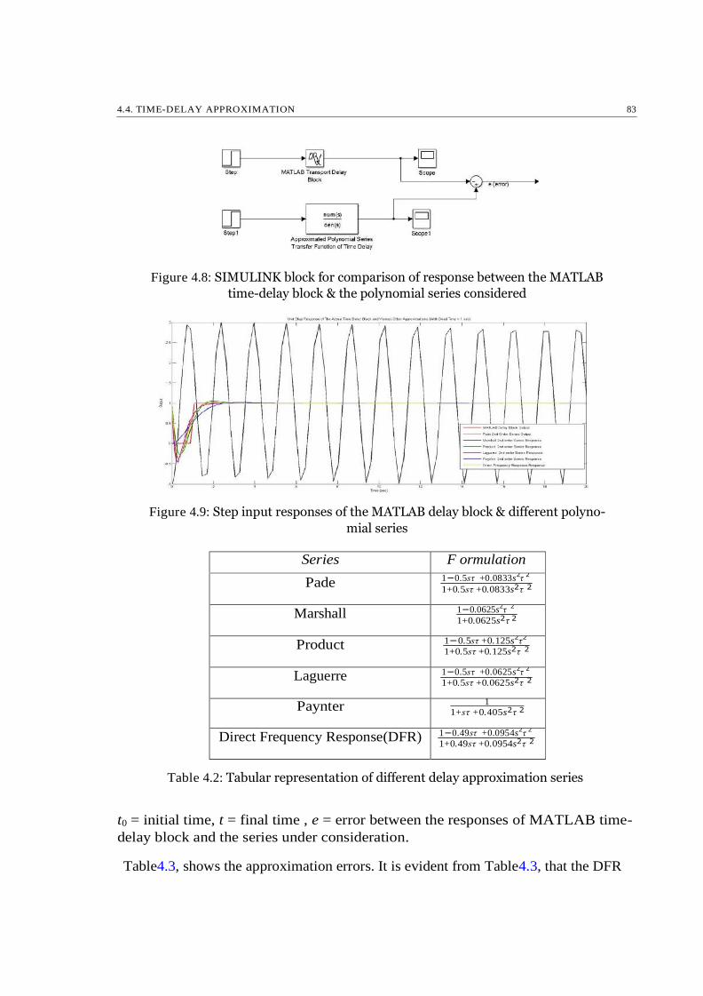
4.4. TIME-DELAY APPROXIMATION 83
Figure 4.8: SIMULINK block for comparison of response between the MATLAB
time-delay block & the polynomial series considered
Figure 4.9: Step input responses of the MATLAB delay block & different polyno-
mial series
Series F ormulation
Pade 1−0.5sτ +0.0833s2τ
2 1+0.5sτ +0.0833s2τ 2
Marshall 1−0.0625s2τ 2 1+0.0625s2τ 2
Product 1−0.5sτ +0.125s2τ 2 1+0.5sτ +0.125s2τ 2
Laguerre 1−0.5sτ +0.0625s2τ 2 1+0.5sτ +0.0625s2τ 2
Paynter 1 1+sτ +0.405s2τ 2
Direct Frequency Response(DFR) 1−0.49sτ +0.0954s2τ 2 1+0.49sτ +0.0954s2τ 2
Table 4.2: Tabular representation of different delay approximation series
t0 = initial time, t = final time , e = error between the responses of MATLAB time-
delay block and the series under consideration.
Table4.3, shows the approximation errors. It is evident from Table4.3, that the DFR

TIME DELAY MEASUREMENT, ESTIMATION, APRROXIMATION & SMITH PREDICTOR SCHEME FOR
DELAY COMPENSATION 84
Series τ = 0.04s τ = 0.120s τ = 0.240s τ = 0.300s τ = 1s AverageISE
Pade 0.0057 0.0172 0.0345 00.0431 0.1437 0.0592
Marshal 43.9888 41.6051 41.1387 40.9687 41.8798 41.321
Product 0.0054 0.0161 0.0321 0.0402 0.1339 0.05516
Laguare 0.0068 0.0203 0.0406 0.0507 0.169 0.06964
Paynter 0.0058 0.0174 0.0347 0.0434 0.1447 0.05962
DFR 0.0053 0.016 0.0319 0.0399 0.1331 0.05482
Table 4.3: Delay approximation errors
series gives the minimum average error followed by the Product series and the Pade
series. Therefore, the DRF series has the best performance among the six series. The
difference between the average errors of the Pade series and the Product series is not
significant. Therefore, for the purpose practical implementation, we choose the DFR
series and Pade series. Though Product series yields less average error in comparison
to Pade, we still consider it as it is one of the widely used polynomial series for delay
approximation.
4.5 Implementation of the Approximated Time-Delay
The matter of our concern is implementation. For the kind of solution we sought after
for the given problem on delay mitigation, it is required to implement the delay polyno-
mial on the embedded platform. This is the reason behind approximating the delay in
form of a polynomial series which can be easily implemented on the embedded device.
The formulation of the solution includes conjunction of delay transfer function and a
compensation scheme which has been discussed in a later chapter. In this section, we
illustrate how the delay polynomial series can be implemented on the embedded de-
vice. Different polynomial series has been depicted in Table4.2. However, as discussed
before, we choose Pade series and the DFR series which are in continuous/analog do-
main. To implement them on the hardware, one has to obtain the discrete version of
them. More specifically, a difference equation form from the continuous form of the
series has to be obtained which can be achieved through a proper transform operation.
One such transform is Bilinear Transform, also known as Tustin’s method or Mobius
Transformation.
In areas of digital signal processing and discrete-time domain control theory, the bi-
linear transform is widely used for transformation of continuous-time domain system
representation to discrete-time and vice-versa [10]. The bilinear transform is a first-
order approximation of the natural logarithm function that is an exact mapping of
the z-plane to the s-plane [10]. For a discrete-time domain signal which has elements
of the discrete-time sequence in conjugation with a delayed unit impulse, the Laplace

4.5. IMPLEMENTATION OF THE APPROXIMATED TIME-DELAY 85
τ
←
. Σ |
T ransform of such a sequence results in the Z-transform of the discrete-time domain
sequence under consideration with the substitution of [10],
Z = e
τds
eτds/2
=
e−τds/2
1 + τds/2
(4.4)
≈ 1 − τds/2
Where,
τd = sampling period.
Now,4.4can be solved for s on a similar consideration for s = 1 ln(z). Therefore, the d
first-order bilinear approximation is,
1 s = ln(z)
τd
= 2
Σ z − 1
+ 1 .
z − 1 Σ3
1 .
z − 1 Σ5
1 .
z − 1 Σ7
+ ...
Σ
τd z + 1 3 z + 1 5 z + 1 7 z + 1 (4.5) 2 z − 1
τd z + 1 2 1 − z
−1
= τd 1 + z−1
Therefore, given a transfer function, G(s), its bilinear transform is given by,
s 2 z − 1
τd z + 1
(4.6)
which results in,
G(z) = G(s) s= 2 z−1 τd z+1
= G 2 z − 1 (4.7)
τd z + 1
Here, we present an example considering Pade first order approximation given as,
≈
+ +

TIME DELAY MEASUREMENT, ESTIMATION, APRROXIMATION & SMITH PREDICTOR SCHEME FOR
DELAY COMPENSATION 86
≈
d
←
d −
−
−
d d d
eτds 2 − τds
2 + τds 4
Gd(s) = 2 + τ s
− 1
(4.8)
Now,
s 2 z − 1
τd z + 1
(4.9)
Substituting τd = 0.02s in (4.9), we obtain,
s = 2 z − 1
0.02 z + 1
= 100 z − 1
z + 1
Now, substituting (4.10) in (4.8), we obtain,
(4.10)
4 Gd(z) =
2 + 100τ
z 1
z+1
− 1 (4.11)
Through algebraic manipulation we can obtain,
G (z) = (2 − 100τd)z + (2 + 100τd)
(4.12)
(2 + 100τ )z + (2 − 100τ )
similarly, the Z domain transformed model of the other series under consideration
can be obtained.
Once the Z domain model is obtained, for formulation of the solution, it will be used
in conjugation with the adopted compensation scheme to mitigate the effects of delay.
The overall formulation and the compensation scheme has been discussed in a later
section.

4.6. INTRODUCTION TO SMITH PREDICTOR 87
4.6 Introduction to Smith Predictor
A time delay is defined as the time difference between the start of an event at one point
of a system and its resulting action at another point of the system [14]. Time delays
are also called as transport lags or dead times [14]. Time delays may arise in physi-
cal,electric, pneumatic, hydraulic networks, chemical processes, long transmission lines,
robotics, biological and economic systems, and also in measurement and computation
[12,14]. Time delay occurs due to some phenomena as given below [13]:
• The time required to transport mass, energy or information.
The accumulation of time lags in a significant numbers of low order systems
connected in series.
• The required processing time for sensors.
Time needed by controllers to implement a complicated control algorithms or
process.
PID controllers are the most widely used controllers in process industries [14]. They
comprise 90-95% of the total controllers used in process industries [14]. However, PID
controllers are less effective when there is dominant time delay in the process dynamics
[14]. Predictive control is necessary if high performance is needed for a process with
significant time delay [13].Smith predictor structure was first proposed by O.J. Smith to
compensate systems with time delay in 1957. For servo applications, a PID controller
with smith predictor serves up to 30% better than a appropriately tuned PID controller
without smith predictor [14]. Smith predictor is a method which does reduction in the
dominance of the time delay term in the closed loop characteristic equation thereby
allowing us to design a controller for the nondominant time delay process [14]. For an
optimally tuned system, an introduction in time delay requires reduction in system gain
to ensure stability [17]. The Smith predictor algorithm helps in avoiding this reduction
in gain and hence the resulting poorer performance [17].
4.7 The Smith Predictor Scheme
The block diagram of a typical Smith predictor scheme is show in Figure4.10as per
[14,17] without considering any.external disturbances The Smith predictor scheme can
be rearranged as shown in Figure4.11. Here, G(s) represents the nominal plant model,
τm represents measured or modeled plant delay, Gc(s) represents the controller along
with actual plant & time delay denoted as G(s) & τd respectively.
•
•

TIME DELAY MEASUREMENT, ESTIMATION, APRROXIMATION & SMITH PREDICTOR SCHEME FOR
DELAY COMPENSATION 88
^
Figure 4.10: Block diagram of a typical Smith predictor scheme
Figure 4.11: Rearranged form of the typical Smith predictor scheme
Now, let the controller with the inner loop as represented in Figure4.11is represented
as Gs(s). Then,
Gc(s) Gs(s) =
(4.13) 1 + (1 − e−τms)G(s)Gc(s)
Then the closed loop transfer function becomes of the plant with smith predictor scheme
becomes,
Y (s)
R(s)
Gs(s)G(s)e−τds
=
1 + Gs(s)G(s)e−τds
(4.14)
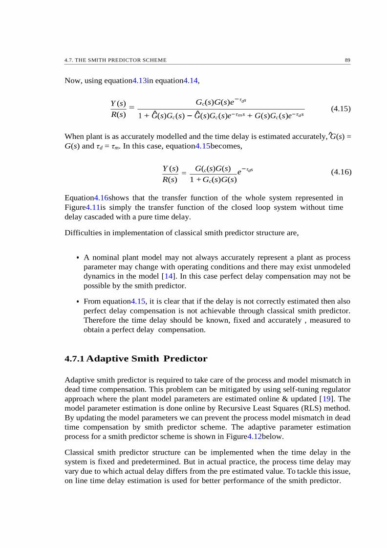
4.7. THE SMITH PREDICTOR SCHEME 89
^
Now, using equation4.13in equation4.14,
Y (s)
R(s)
Gc(s)G(s)e−τds
=
1 + G(s)Gc(s) − G(s)Gc(s)e−τms + G(s)Gc(s)e−τds
(4.15)
When plant is as accurately modelled and the time delay is estimated accurately, G(s) =
G(s) and τd = τm. In this case, equation4.15becomes,
Y (s) =
G(c(s)G(s)
e−τds (4.16)
R(s) 1 + Gc(s)G(s)
Equation4.16shows that the transfer function of the whole system represented in
Figure4.11is simply the transfer function of the closed loop system without time
delay cascaded with a pure time delay.
Difficulties in implementation of classical smith predictor structure are,
A nominal plant model may not always accurately represent a plant as process
parameter may change with operating conditions and there may exist unmodeled
dynamics in the model [14]. In this case perfect delay compensation may not be
possible by the smith predictor.
From equation4.15, it is clear that if the delay is not correctly estimated then also
perfect delay compensation is not achievable through classical smith predictor.
Therefore the time delay should be known, fixed and accurately , measured to
obtain a perfect delay compensation.
4.7.1 Adaptive Smith Predictor
Adaptive smith predictor is required to take care of the process and model mismatch in
dead time compensation. This problem can be mitigated by using self-tuning regulator
approach where the plant model parameters are estimated online & updated [19]. The
model parameter estimation is done online by Recursive Least Squares (RLS) method.
By updating the model parameters we can prevent the process model mismatch in dead
time compensation by smith predictor scheme. The adaptive parameter estimation
process for a smith predictor scheme is shown in Figure4.12below.
Classical smith predictor structure can be implemented when the time delay in the
system is fixed and predetermined. But in actual practice, the process time delay may
vary due to which actual delay differs from the pre estimated value. To tackle this issue,
on line time delay estimation is used for better performance of the smith predictor.
•
•
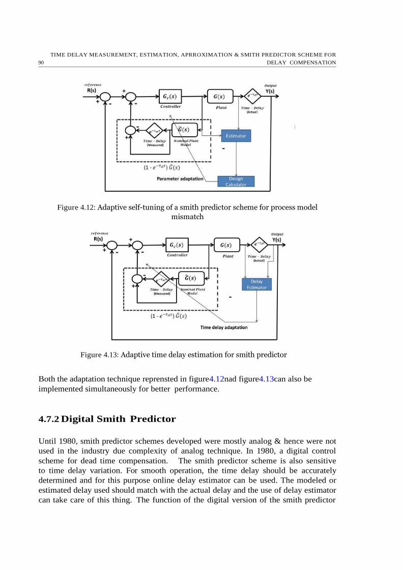
TIME DELAY MEASUREMENT, ESTIMATION, APRROXIMATION & SMITH PREDICTOR SCHEME FOR
DELAY COMPENSATION 90
Figure 4.12: Adaptive self-tuning of a smith predictor scheme for process model
mismatch
Figure 4.13: Adaptive time delay estimation for smith predictor
Both the adaptation technique reprensted in figure4.12nad figure4.13can also be
implemented simultaneously for better performance.
4.7.2 Digital Smith Predictor
Until 1980, smith predictor schemes developed were mostly analog & hence were not
used in the industry due complexity of analog technique. In 1980, a digital control
scheme for dead time compensation. The smith predictor scheme is also sensitive
to time delay variation. For smooth operation, the time delay should be accurately
determined and for this purpose online delay estimator can be used. The modeled or
estimated delay used should match with the actual delay and the use of delay estimator
can take care of this thing. The function of the digital version of the smith predictor

4.8. IMPLEMENTATION OF DIGITAL SMITH PREDICTOR IN WNCS 91
is similar to the classical version with similar functionality of the different blocks in
discrete domain. The basic digital smith predictor structure is shown in figure ??.
Here, all the blocks are represented in discrete domain similar like in the analog type.
It is important to note that the actual delay is shown as Gd(z) (discrete transformation
of e−τds) and the estimated delay is shown as Gdm(z) (discrete transformation of
e−τms).
Figure 4.14: Digital smith predictor structure [19]
The scheme represented in figure4.14is be rearranged and shown in figure4.16.
Figure 4.15: Rearranged form of the digital smith predictor represented in figure
4.14
4.8 Implementation of Digital Smith Predictor in
WNCS
In a earlier chapter we have discussed estimation of time delay in WNCS using round
trip time (RTT) concept. The network induced time delay in point to point configura-
tion of two Bluetooth node is found to be 0.06 second most of the time. Hence, we have

TIME DELAY MEASUREMENT, ESTIMATION, APRROXIMATION & SMITH PREDICTOR SCHEME FOR
DELAY COMPENSATION 92
− ^
taken 0.06 second as the dead time for implementation of smith predictor structure as
per the scheme represented in figure4.16.
Here the nominal plant model is taken as the discretized transfer function of the DC
motor model cascaded with the ZOH block. The nominal plant model used in smith
predictor block is given as,
G(z −1) = 0.0832z−1
1 − 0.92z−1
(4.17)
Now for implementation in embedded platform, the delay block need to be represented
as a discrete transfer function. For this purpose, we have done system identification of
the MATLAB transport delay block as shown in figure4.16.
Figure 4.16: Data collection in SIMULINK for identification of delay block transfer
function
Now the identified delay block discrete transfer function with best fitting (in feasible
order) is obtained from MATLAB system identification toolbox as,
Gd(z 0.0006313z
−1 + 0.000636z
−2 + 0.9971z
−3
−1) = (4.18) 1 − 0.0006345z−1 − 0.000633z−2 + 0.00007223z−3
Now using the (1 Gd(z−1
))G(z−1
) block as diifference equation in embedded micro
controller as shown in figure4.17, we have implemented the smith predictor scheme.
The practical response of the plant with discrete PI controller without smith predictor
scheme for the point-to-point network configuration has been shown in figure4.18.
Now the practical response of the plant with digital smith predictor scheme has been
shown in figure4.19.
It has been observed that with the implementation of digital smith predictor scheme in
wireless point-to-point congiguration of the servo system, good performance is obtained
compared to conventional PI controller when there is a fixed network induced time delay
of 0.06 second.

4.8. IMPLEMENTATION OF DIGITAL SMITH PREDICTOR IN WNCS 93
Figure 4.17: Implemented digital smith predictor scheme for the wireless point-to-
point configuration
Figure 4.18: Practical response and control signal without smith predictor scheme
in wireless point-to-point configuration
4.8.1 Digital Smith Predictor With Intermediate Communi-
cation Nodes
We can see that the digital smith predictor scheme implemented for point-to-point
Bluetooth networked servo system works fine as the delay is fixed. But when interme-
diate two nodes are inserted between the controller node and plant side node, the time
delay no longer remains fixed and it varies from 0.06 second delay in the point to point
case. In this network configuration we observe the response of the servo system for two
time with the digital smith predictor.

TIME DELAY MEASUREMENT, ESTIMATION, APRROXIMATION & SMITH PREDICTOR SCHEME FOR
DELAY COMPENSATION 94
Figure 4.19: Practical response and control signal with smith predictor scheme in
wireless point-to-point configuration
Figure 4.20: Practical response with smith predictor scheme in network having
intermediate nodes (1st time)
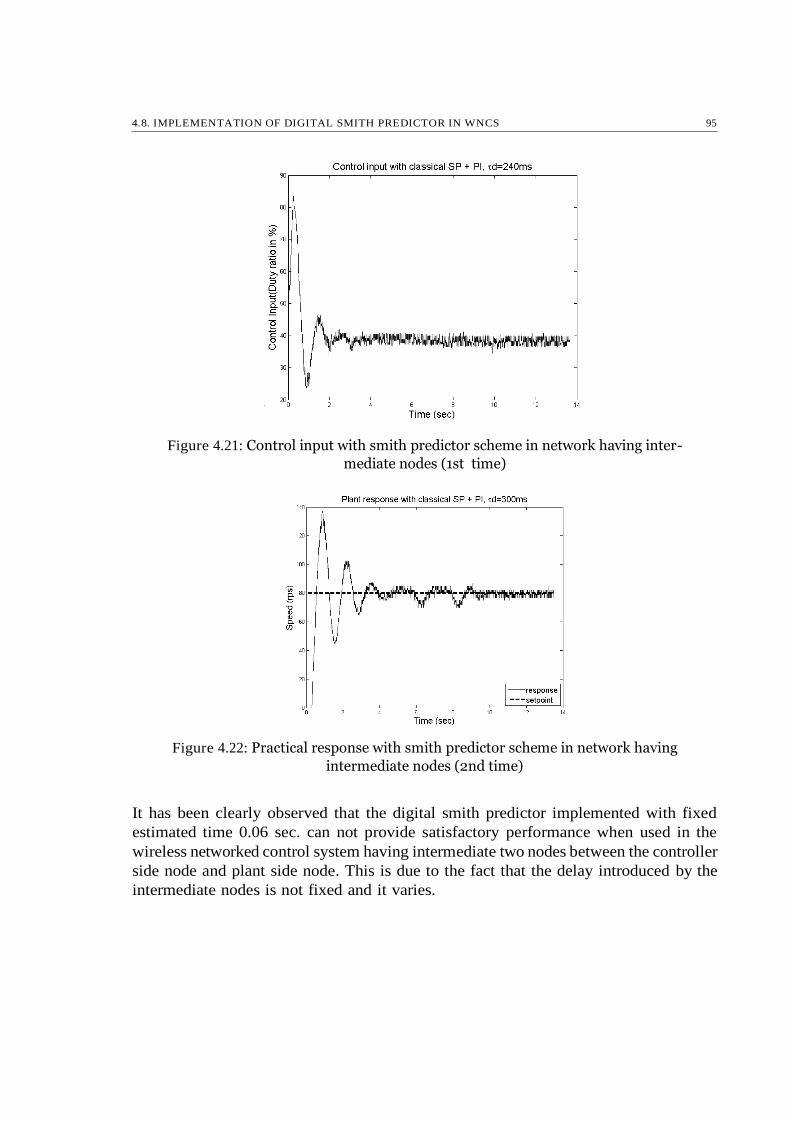
4.8. IMPLEMENTATION OF DIGITAL SMITH PREDICTOR IN WNCS 95
Figure 4.21: Control input with smith predictor scheme in network having inter-
mediate nodes (1st time)
Figure 4.22: Practical response with smith predictor scheme in network having
intermediate nodes (2nd time)
It has been clearly observed that the digital smith predictor implemented with fixed
estimated time 0.06 sec. can not provide satisfactory performance when used in the
wireless networked control system having intermediate two nodes between the controller
side node and plant side node. This is due to the fact that the delay introduced by the
intermediate nodes is not fixed and it varies.

TIME DELAY MEASUREMENT, ESTIMATION, APRROXIMATION & SMITH PREDICTOR SCHEME FOR
DELAY COMPENSATION 96
Figure 4.23: Control input with smith predictor scheme in network having inter-
mediate nodes (2nd time)
4.8.2 Adaptive Digital Smith Predictor
As the performance of the digital smith predictor scheme with fixed estimated time de-
lay can not provide satisfactory response when dead time is varying, therefore adaptive
smith predictor scheme is needed. The performance of smith predictor significantly
degrades (may become unstable) due to modeling or estimation errors of both delay
and process [16]. Specially dead time estimation error is very dangerous as it can vary
widely depending on working conditions [16]. Therefore we are not using parameter
adaptation of the process model while implementing the adaptive digital smith predic-
tor. The adaptive smith predictor proposed here simply updates the process time delay
as measured and estimated on line by the method discussed in an earlier chapter. The
adaptive digital smith predictor proposed is given in figure4.24.
Here, Gd(z) is the discrete delay model implemented in the embedded computer. Here
we are using both discrete 2nd order Pade series and Direct Frequency Response (DFR)
series approximation for the estimated time delay. The discretization of the polynomial
series has been discussed in a earlier chapter. Therefore the 2nd order discrete DFR
series approximation for an estimated time delay τm is given as,
cz2 + dz + e
Gd(df r)(z) = ez2 + dz + c
(4.19)
Where,
c = 1 + 100 τm(9.54τm − 0.49)
d = 2 - 100 τm(9.54τm + 0.49) − 100τm(9.54τm − 0.49)
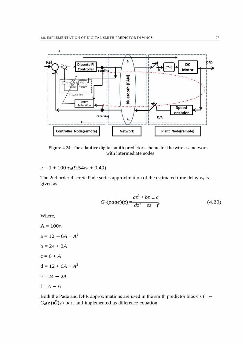
4.8. IMPLEMENTATION OF DIGITAL SMITH PREDICTOR IN WNCS 97
−
Figure 4.24: The adaptive digital smith predictor scheme for the wireless network
with intermediate nodes
e = 1 + 100 τm(9.54τm + 0.49)
The 2nd order discrete Pade series approximation of the estimated time delay τm is
given as,
az2 + bz c
Gd(pade)(z) = dz2 + ez + f
(4.20)
Where,
A = 100τm
a = 12 − 6A + A2
b = 24 + 2A
c = 6 + A
d = 12 + 6A + A2
e = 24 − 2A
f = A − 6
Both the Pade and DFR approximations are used in the smith predictor block’s (1 −
Gd(z))G(z) part and implemented as difference equation.

TIME DELAY MEASUREMENT, ESTIMATION, APRROXIMATION & SMITH PREDICTOR SCHEME FOR
DELAY COMPENSATION 98
Figure 4.25: Response with Pade series delay approximation of the adaptive digital
smith predictor in wireless network with intermediate nodes
Figure 4.26: Control input with Pade series delay approximation of the adaptive
digital smith predictor in wireless network with intermediate nodes
Figure 4.27: Response with DFR series delay approximation of the adaptive digital
smith predictor in wireless network with intermediate nodes

4.8. IMPLEMENTATION OF DIGITAL SMITH PREDICTOR IN WNCS 99
Figure 4.28: Control input with DFR series delay approximation of the adaptive
digital smith predictor in wireless network with intermediate nodes
4.8.3 Implementation of Discrete Transfer Function in Em-
bedded Platform
The Pade and DFR discrete domain approximation series are often very long, hence
we are showing a simplified example transfer function showing the implementation.
Let us consider a simple discrete transfer function,,
2z G(z) = (4.21)
z2 − z + 1
The we can also represent the transfer function as,
G(z −1) = 2z−1
1 − z−1 + z−2
(4.22)
Now we can represent, the transfer function in terms of discrete input X(k) & output
Y(k) as,
Now,
Y (k)
X(k)
= G(z −1) = 2z−1
1 − z−1 + z−2
(4.23)
⇒ 2z−2
X(k) = Y (k)(1 − z−1 + z
−2) (4.24)
⇒ 2X(k − 1) = Y (k) − Y (k − 1) + Y (k − 2) (4.25)
⇒ Y (k) = 2X(k − 1) + Y (k − 1) − Y (k − 2) (4.26)

TIME DELAY MEASUREMENT, ESTIMATION, APRROXIMATION & SMITH PREDICTOR SCHEME FOR
DELAY COMPENSATION 100
−
Equation4.26provides the difference equation of the discrete transfer function G(z)
which can be implemented in embedded controller. In this way the delay approximated
series and the nominal plant model combined transfer function in discrete domain
((1 Gdm(z))G(z)) has been implemented in embedded controller to get smith predictor
action.
4.9 Practical Waveforms Obtained from Extensive
Experimentation of the Digital Smith Predictor
Figure 4.29: Response of Classical Digital Smith Predictor + PI controller when
time delay = 80 ms
Figure 4.30: Response of Classical Digital Smith Predictor + PI controller when
time delay = 240 ms

4.9. PRACTICAL WAVEFORMS OBTAINED FROM EXTENSIVE EXPERIMENTATION OF THE DIGITAL
SMITH PREDICTOR 101
Figure 4.31: Response of Classical Digital Smith Predictor + PI controller when
time delay = 300 ms
Figure 4.32: Response of Classical Digital Smith Predictor + PI controller when
time delay = 400 ms
Figure 4.33: Response of Adaptive Digital Smith Predictor( DFR approx.) + PI
controller when time delay = 240 ms

TIME DELAY MEASUREMENT, ESTIMATION, APRROXIMATION & SMITH PREDICTOR SCHEME FOR
DELAY COMPENSATION 102
Figure 4.34: Response of Adaptive Digital Smith Predictor( DFR approx.) + PI
controller when time delay = 300 ms
Figure 4.35: Response of Adaptive Digital Smith Predictor( DFR approx.) + PI
controller when time delay = 400 ms
Figure 4.36: Response of Adaptive Digital Smith Predictor( Pade approx.) + PI
controller when time delay = 240 ms
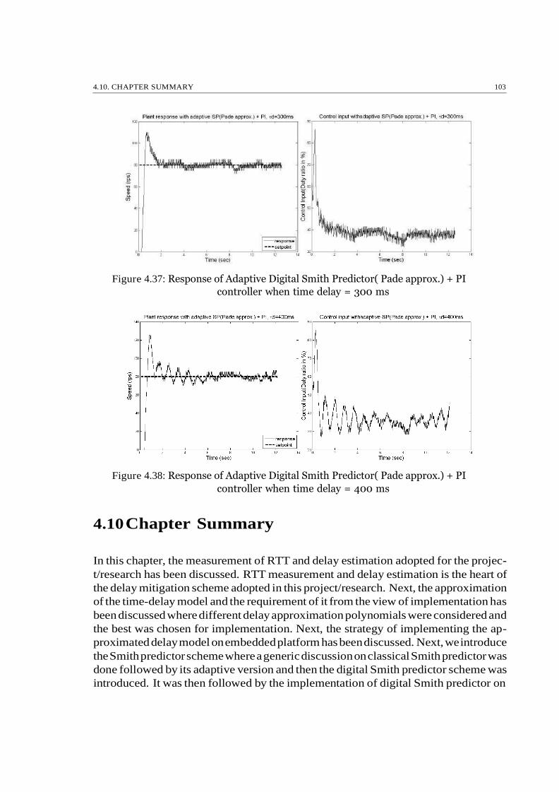
4.10. CHAPTER SUMMARY 103
Figure 4.37: Response of Adaptive Digital Smith Predictor( Pade approx.) + PI
controller when time delay = 300 ms
Figure 4.38: Response of Adaptive Digital Smith Predictor( Pade approx.) + PI
controller when time delay = 400 ms
4.10 Chapter Summary
In this chapter, the measurement of RTT and delay estimation adopted for the projec-
t/research has been discussed. RTT measurement and delay estimation is the heart of
the delay mitigation scheme adopted in this project/research. Next, the approximation
of the time-delay model and the requirement of it from the view of implementation has
been discussed where different delay approximation polynomials were considered and
the best was chosen for implementation. Next, the strategy of implementing the ap-
proximated delay model on embedded platform has been discussed. Next, we introduce
the Smith predictor scheme where a generic discussion on classical Smith predictor was
done followed by its adaptive version and then the digital Smith predictor scheme was
introduced. It was then followed by the implementation of digital Smith predictor on

104 REFERENCES
embedded hardware where a constant delay model scheme for Smith predictor was dis-
cussed. It was observed that the Smith predictor as a constant delay model did not
perform well for a significant amount of delay (by introduction of intermediate commu-
nication node). Therefore, an adaptive scheme for the Smith predictor was introduced
where delay was considered to be varying and of significant magnitude. It was here, we
used the approximated delay model in conjugation with the Smith predictor to make
it adaptive, the estimated delay was continuously fed to the Smith predictor block (as
shown in4.24 ) for the required delay compensation. Next, we illustrate the practi-
cal waveforms as obtained from experimentation considering different Smith predictor
schemes. It was observed that, the DFR series approximation of delay gave better result
when compared to Pade approximation polynimial of delay.
References
[1] Lai, C.L. and Hsu, P.L., 2010. Design the remote control system with the time-
delay estimator and the adaptive smith predictor. IEEE Transactions on Industrial
Informatics, 6(1), pp.73-80.
[2] Suryendu, C., Ghosh, S. and Subudhi, B., 2017. Variable Gain Output Feedback
Control of A Networked Temperature Control System Based on Online Delay Esti-
mation. Asian Journal of Control.
[3] De Boeij, J., Haazen, M., Smulders, P. and Lomonova, E., 2009. Low-latency wire-
less data transfer for motion control. Journal of Control Science and Engineering,
2009, p.3
[4] Chhavi Suryendu, Time-Delay Estimation Based Wireless-Networked Temperature
Control System Department of Electrical Engineering, National Institute of Tech-
nology Rourkela, M.Tech thesis
[5]J. P. Hespanha, P. Naghshtabrizi, and Y. Xu, A survey of recent results in networked
control systems, Proceedings of the IEEE, vol. 95, no. 1, 2007.
[6] Wang, R., Liu, G.P., Wang, W., Rees, D. and Zhao, Y.B., 2010. Guaranteed cost
control for networked control systems based on an improved predictive control
method. IEEE Transactions on Control Systems Technology, 18(5), pp.1226-1232.
[7] Wikipedia contributors. ”Round-trip delay time.” Wikipedia, The Free Encyclope-
dia. Wikipedia, The Free Encyclopedia, 12 Apr. 2017. Web. 21 Apr. 2017.
[8] Leonid Mirkin, Faculty of Mechanical Engineering, TechnionIsrael Institute of Tech-
nology, Department of Automatic Control, Lund University
[9] Mirzal, A., 2012. Stability analysis and compensation of time delays in analog
control systems. Int’l J. Control and Automation , 5(4), pp.1-18.

REFERENCES 105
[10] Wikipedia contributors. ”Bilinear transform.” Wikipedia, The Free Encyclopedia.
Wikipedia, The Free Encyclopedia, 23 Feb. 2017. Web. 9 May. 2017.
[11] Bobl, V., Chalupa, P., Dostl, P. and Kubalk, M., 2014. Digital Smith Predictor
for Control of Unstable and Integrating Time-delay Processes. In Proceedings of
the 2014 international conference on mechatronics and robotics, structural analysis
(MEROSTA 2014), Santorini Island, Greece (pp. 105-110).
[12] Bobl, V., Matunu, R. and Dostl, P., 2011, June. Digital Smith Predictors-Design
And Simulation Study. In ECMS (pp. 480-486).
[13] Bobl, V., Chalupa, P., Dostl, P. and Kubalk, M., 2011, May. Adaptive digital
Smith predictor. In Recent Researches in Automatic Control-13th WSEAS Interna-
tional Conference on Automatic Control, Modelling and Simulation, ACMOS’11.
[14] O’Dwyer, Aidan : A reference guide to Smith predictor based methods for the
compensation of dead-time processes. Proceedings of the IEE Irish Signals and Sys-
tems Conference, pp. 231-238, Dublin City University, September, 2005.
[15] Sourdille, Pauline and O’Dwyer, Aidan : An outline and further development of
Smith predictor based methods for the compensation of processes with time delay.
Proceedings of the Irish Signals and Systems Conference, pp. 338-343, University of
Limerick, July, 2003.
[16] Massimiliano, V., 2003. Performance improvement of Smith Predictor through
automatic computation of dead time. Yokogawa Technical Report, pp.25-30.
[17] Bahill, A., 1983. A simple adaptive smith-predictor for controlling time-delay sys-
tems: A tutorial. IEEE Control systems magazine, 3(2), pp.16-22.
[18] Deshpande, P. B. and Ash, R. H., 1981. Elements of Computer Process Control
With Advanced Control Applications. Research Triangle Park NC: Instrument So-
ciety of America, 1981. pp. 227-250.
[19] Hang, C.C., Lim, K.W. and Chong, B.W., 1989. A dual-rate adaptive digital Smith
predictor. Automatica, 25(1), pp.1-16.

Chapter 5
Stability Analysis of the DC Motor
System
5.1 Introduction
In this chapter, we illustrate a qualitative analysis on the stability of the system under
consideration with different time delays. Within a system, Dead-time / time delay is
the time interval between an event initiated at a point in the system and the output of
that event at another point in the same system [1]. The stability of a minimum phase
system (systems that do not have poles or zeros in the right-hand side of s-plane or do
not have other delay component ) is always found to be reduced with inclusion of delay
in the system [1]. Therefore, under the presence of delay, the stability analysis of a
system is vital.
5.2 Nyquist Stability Criterion for System with Time
Delays
In system engineering, stability of closed-loop system is a basic concept as only this
type of system has practical use [1]. A system is said to be stable if it generates bounded
output for bounded inputs [2]. The benefits of analyzing the stability of a system in
frequency domain, according to [3], are :
• Simple stability tests and improved accuracy with sinusoidal signal generator.
• Experimentally, frequency response tests can provide complex transfer functions.
107

108 STABILITY ANALYSIS OF THE DC MOTOR SYSTEM
Design & analysis process are extendable to non-linear systems by neglecting
noise effects.
The Nyquist stability criterion provides us the stability of a closed-loop system from
its corresponding open-loop frequency response and open-loop poles [2]. Both absolute
and relative stability analysis can be done with Nyquist stability criterion [1]. The
presence of dead time in the system does not alter the criterion, and therefore it can
be utilized for analysis of stability of systems with time-delay [1].
Let us first consider a closed loop system free from time delay,
Gp(s) G(s) =
1 + Gp(s)H(s)
(5.1)
Then, the Nyquist stability criterion is given by,
Z = N + P
where,
Z= the number of zeros of 1+G(s)H(s) on the right hand part of the s-plane,
N = the number of locus of G(j)H(j) that encircles point −1 + j0 clockwise,
P = denotes the number of poles of G(s)H(s) on the right hand part of the s-plane
Now, if delay is introduced, the characteristic equation can be written as,
X(s) = 1 + Gp(s)H(s)e−τds = 0 (5.2)
Now, let,
d(s) = X(s) − 1 = Gp(s)H(s)e−τds = 0 (5.3)
Cauchy theorem states that contour integral of d(s) along closed path on the s-plane
equals to zero if D(s) is analytic both inside and along the path. Therefore,
I
C
d(s)ds = 0 (5.4)
•

5.2. NYQUIST STABILITY CRITERION FOR SYSTEM WITH TIME DELAYS 109
d(s)
I
d(s) −
with the integral evaluated in clockwise direction. Now, expressing d(s) in terms of its
poles and zeroes, we arrive at a decomposed form of d(s) given by,
d(s) =
(s + z1)l1 (s + z2)
l2 ...
s + p1)o1 (s + p2)o2 ...
e−τds
(5.5)
Now, the ratio dj(s)
is written as,
dj(s)
=
. l1
+ l2
+ ...
Σ
−
. o1
+
+ ...
Σ
− τd
(5.6)
1 2 1
Using residual theorem,
dj(s)
= 2πj[(l1 C
+ l1 + ...) − (o1
+ o2
+ ...)]
(5.7)
= −2πj(Z − P )
where,
Z = the number of zeros of d(s) inside the path,
P = the number of and poles of d(s) inside the path
Since d(s) is a complex variable, it can be expressed as,
d(s) = |d(s)|ejθ
=⇒ ln(d(s)) = ln|d(s)| + jθ
(5.8)
Therefore,
dj(s)
d(s)
dlnd(s) =
ds
= dln|d(s)|
+ jθ
ds
(5.9)
m2
d(s) s + z s + z s + p s + p2

110 STABILITY ANALYSIS OF THE DC MOTOR SYSTEM
I
|
hence,
d
j(s)
=
C d(s)
dln|d(s)| + j
I
dθ
(5.10)
= 2π(P − Z)
where, I
dln|d(s)| = 0 (5.11)
as ln d(s) has an equal value on the initial and the end point of the integration. Ac-
cordingly,
θ2 − θ1
2π = P − Z (5.12)
The angular difference between end point and initial point of θ equals to the total
change in the phase angle of d’(s)/d(s). As N denotes the number of closed paths on
d(s) plane that encircle the original point in clockwise manner, and θ2-θ1 = 2πl, l =
0,1,...., then
θ2 − θ1
2π = −N
(5.13)
=⇒ N = Z − P
Therefore, the existence of delay does not alter the Nyquist Stability criterion. Thus,
it can be used for systems with time-delays.
Analysis of stability of a linear system with Nyquist stability criterion leads to the
following possibilities [[1],[2],
System is stable if there is no encirclement of the point -1+j0 by the closed path
on G(s)H(s) plane, provided there is no pole of G(s)H(s) on the right hand side
of the s-plane.
C
C
C C
•
I

5.2. NYQUIST STABILITY CRITERION FOR SYSTEM WITH TIME DELAYS 111
System is stable if there are one or more counter-clockwise encirclement of the
point -1+j0 by the closed path on G(s)H(s) plane, provided the number of counter-
clockwise encirclement is equal to the number of poles of G(s)H(s) in the right-half
of s-plane. Otherwise, system is unstable.
System is unstable if there are one or more clockwise encirclement of the point
-1+j0 by the closed path on G(s)H(s) plane.
Figure 5.1: Nyquist plot(a) & polar plot(b) for the open-loop transfer function
tt(s)H(s) without time-delay
For the system under consideration, the open-loop transfer function is given by,
4.159
G(s)H(s) = s + 3.888
(5.14)
The Nyquist & polar plot of equation5.14is shown in figure5.1.From figure5.1, it is
clear that the open-loop transfer function G(s)H(s) of the plant is absolutely stable in
closed-loop configuration as there is neither zero nor pole lies on the right hand side of
the s-plane and locus of G(s)H(s) does not encircle the point -1+j0.
An important concept of stability analysis is relative stability which is related with the
settling time [1]. Faster settling time of a system implies better stability compared to
a system with slower settling time . Degree of stability of a system can be determined
with the help of Nyquist plot and polar plot. The relative stability based on the
distance of G(j)H(j) locus to -1+j0 point can be stated in the phase margin. The phase
margin is defined as the phase lag that needs to be compensated for the system to be
at the border of stability. Mathematically, the phase margin can be written as,
φM = γ = 180◦ + φ (5.15)
•
•
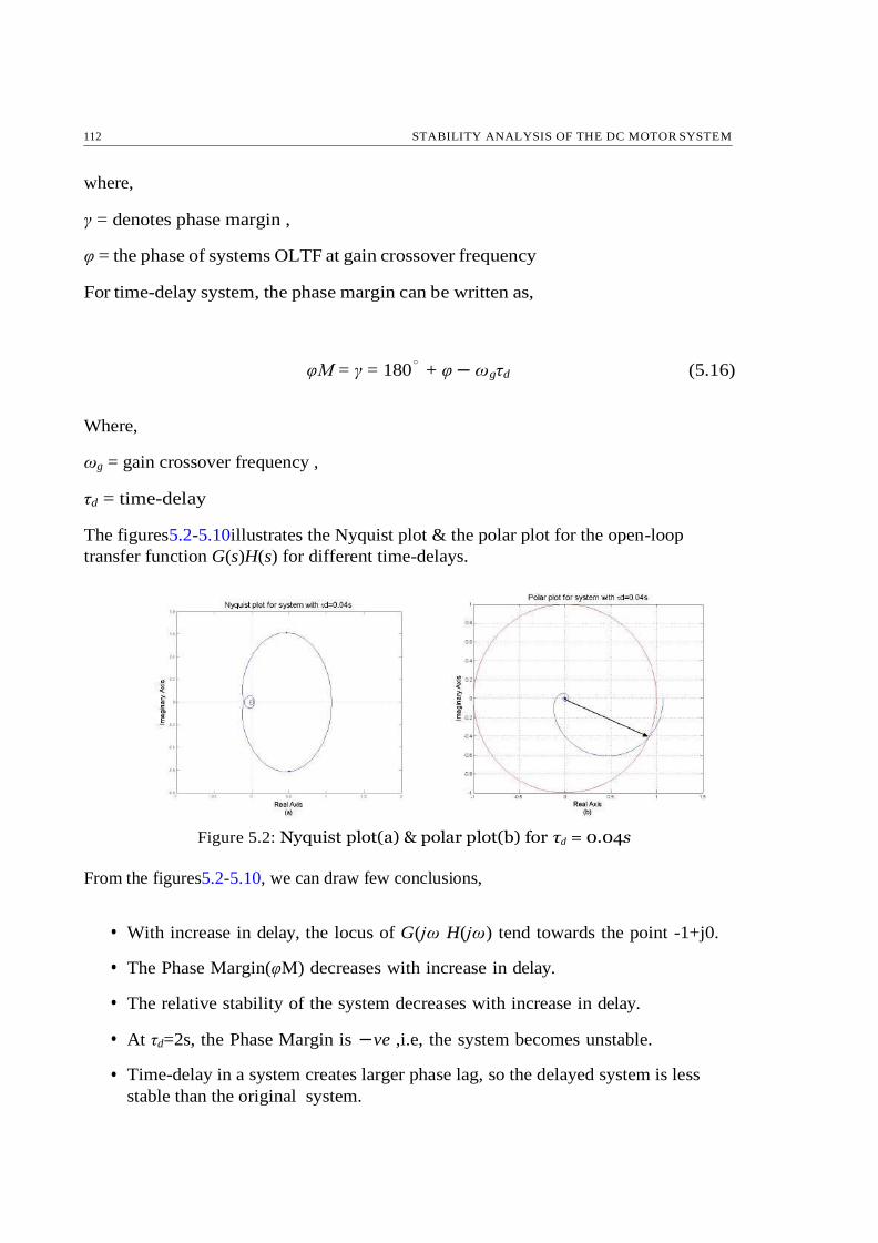
112 STABILITY ANALYSIS OF THE DC MOTOR SYSTEM
where,
γ = denotes phase margin ,
φ = the phase of systems OLTF at gain crossover frequency
For time-delay system, the phase margin can be written as,
φM = γ = 180◦ + φ − ωgτd (5.16)
Where,
ωg = gain crossover frequency ,
τd = time-delay
The figures5.2-5.10illustrates the Nyquist plot & the polar plot for the open-loop
transfer function G(s)H(s) for different time-delays.
Figure 5.2: Nyquist plot(a) & polar plot(b) for τd = 0.04s
From the figures5.2-5.10, we can draw few conclusions,
• With increase in delay, the locus of G(jω H(jω) tend towards the point -1+j0.
• The Phase Margin(φM) decreases with increase in delay.
• The relative stability of the system decreases with increase in delay.
• At τd=2s, the Phase Margin is −ve ,i.e, the system becomes unstable.
Time-delay in a system creates larger phase lag, so the delayed system is less
stable than the original system.
•
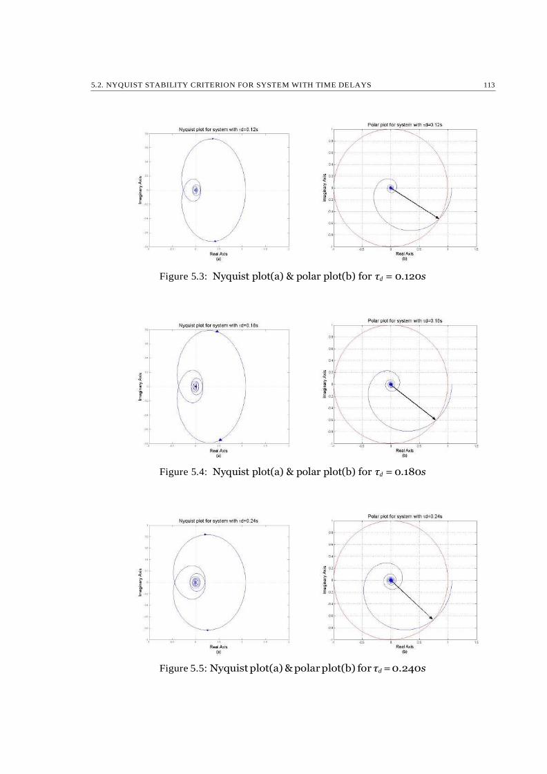
5.2. NYQUIST STABILITY CRITERION FOR SYSTEM WITH TIME DELAYS 113
Figure 5.3: Nyquist plot(a) & polar plot(b) for τd = 0.120s
Figure 5.4: Nyquist plot(a) & polar plot(b) for τd = 0.180s
Figure 5.5: Nyquist plot(a) & polar plot(b) for τd = 0.240s
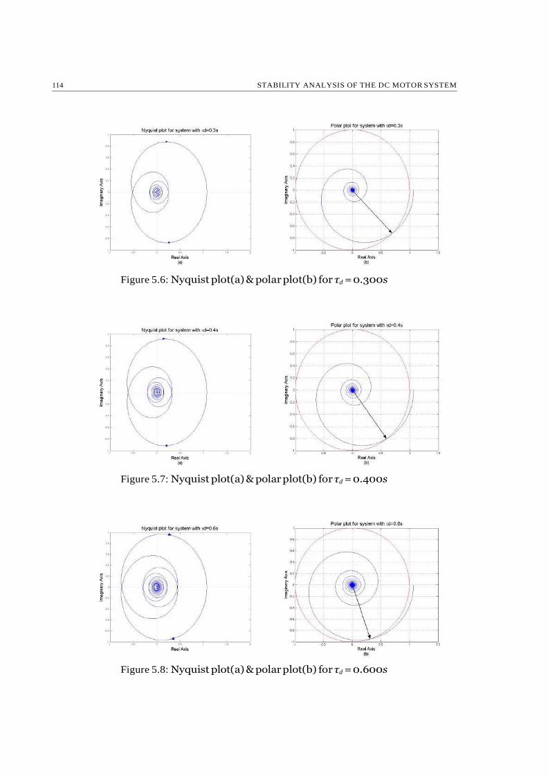
114 STABILITY ANALYSIS OF THE DC MOTOR SYSTEM
Figure 5.6: Nyquist plot(a) & polar plot(b) for τd = 0.300s
Figure 5.7: Nyquist plot(a) & polar plot(b) for τd = 0.400s
Figure 5.8: Nyquist plot(a) & polar plot(b) for τd = 0.600s

5.2. NYQUIST STABILITY CRITERION FOR SYSTEM WITH TIME DELAYS 115
Figure 5.9: Nyquist plot(a) & polar plot(b) for τd = 1s
Figure 5.10: Nyquist plot(a) & polar plot(b) for τd = 2s
Table5.1illustrates the obtained Phase Margin( φM) for the system under consideration
for different time-delays. The Phase Margins were calculated geometrically.
Figure 5.11: Polar plot for different time-delays

116 REFERENCES
T ime − Delay, τd seconds P hase M argin(φM )
0 159.19
0.04 156.68
0.120 148.73
0.180 144.83
0.240 139.30
0.300 134.02
0.400 126.31
0.600 106
1 74.53
2 -10.11
Table 5.1: Variation of φM with variation in τd
5.3 Chapter Summary
In this chapter, a qualitative analysis on the stability of the DC motor system is
illustrated. Here, the stability analysis of the plant done using Nyquist criterion of
stability. Nyquist and polar plots for different time delays were studied. It was observed
that with increase in delay, the phase margin reduced. Therefore, the relative stability
of the plant is reduced with increase in delay.
References
[1]Mirzal, A., 2012. Stability analysis and compensation of time delays in analog
control systems. Int’l J. Control and Automation, 5(4), pp.1-18.
[2]K. Ogata, Modern Control Engineering, 5th edition, Prentice-Hall, (2009).
[3]G. F. Franklin, J. D. Powell and A. Emami-Naeni, Feedback Control of Dynamic
Systems, 3rd edition, Addison-Wesley Publishing Company, (1994).
[4]Ogata, K., 1995. Discrete-time control systems (Vol. 2). Englewood Cliffs, NJ: Pren-
tice Hall.

Chapter 6
Modifications,
Contributions/Proposals of The
Research
Though the strategy of estimation of delay was adopted from [1],necessary modification
in the existing strategy has been made to adopt it to the system under consideration.
The goal was to implement the strategy on the hardware platform (ARDUINO UNO/-
DUE ), hence, modification was necessary for the sake of implementation. Modification
pertaining to refitting the existing idea to comply with the system under consideration
with due concern on the ease of implementation and etiquette of the strategy were
always under consideration.
The modification is given as under,
Modification: In [1], the RTT measurement & estimation of delay was made at
the plant node and then the information of delay was sent to the controller node.
For the system under consideration, i.e, for our system, the RTT measurement
& delay estimation were made at the controller node itself. Necessity for such a
modification,
– If RTT is measured on the plant side, for compensation of the estimated
delay, the information has to be sent to the controller node. Therefore, in
[1], the delay information at each frame was sent to the controller node at
half sampling period and complicated algorithms were designed to achieve
this purpose. Whereas, for the system under consideration, the measurement
and estimation of delay was made at the controller node itself, hence, such
complicated algorithms were avoided. Thus, making the implementation
easier and more convenient.
117
•

118 MODIFICATIONS, CONTRIBUTIONS/PROPOSALS OF THE RESEARCH
Σ
– Measurement of delay at the plant node and then transfer of this informa-
tion to the controller node may itself suffer from delay. If the information of
delay gets delayed itself and does not arrive before the arrival of the feedback
signal, the control action required for the compensation of the delay for that
very sample period may ultimately get delayed and the overall performance
of the system may get degraded. Whereas, for the system under consid-
eration, such an undesirable phenomenon/happening has been avoided by
directly measuring and estimating the delay at the controller node itself.
When it comes down to the level of implementation, especially on a dedicated hardware
platform, two factors are always a matter of concern; namely, The Cost of Imple- mentation & The Ease of Implementation. The implemented idea should be
practical and equally economically viable. A product/idea maintaining a correct ratio
of these two factors is admissible. A growing technology demands for an easy and
cost-effective solution to a given commercial problem. In relation to this, we present
few contributions and proposals put forward by us for an easy and cheap solution to
the problem of delay estimation and mitigation.
The contributions/proposals are listed as under,
In [1], the system runs on a high performance computer supported with sophis-
ticated hardware and software. The control and estimations algorithms were all
implemented on it. The goals were ultimately achieved but the overall cost of
implementation was high. The objective of our project/research was to find a
cheaper alternative to this. Therefore, in order to reduce the cost of implementa-
tion, the control system as a whole was exclusively implemented on a dedicated
hardware where no high performance PC and other sophisticated software were
involved. The cost of the hardware (ARDUINO UNO/DUE) ( 1000 - 1500) is
quite less when compared to a high performance PC. Thus, by bringing down the
implementation on a dedicated hardware gives a compact and economic solution
to the problem that too in form of a device which can be readily used for delay
estimation and compensation.
In the chapter of delay estimation, it was discussed that the delay estimated at
a sampling time is equal to the summation of the difference between the time
stamps (t1&t2) summed for the number of times vacant samples occur after 0ms.
In connection to this observation, we propose an empirical formula for estimation
of delay,
Where,
n
tm = ti (6.1)
i=0
•
•
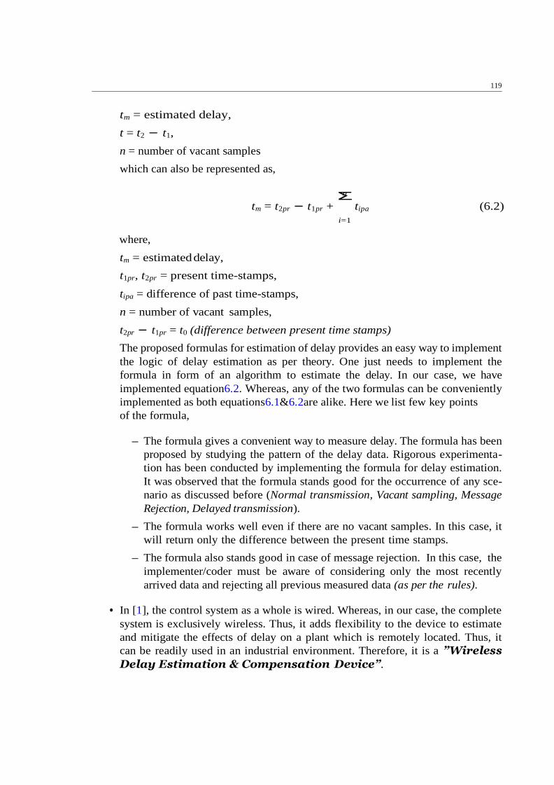
Σ
119
tm = estimated delay,
t = t2 − t1,
n = number of vacant samples
which can also be represented as,
where,
tm = estimated delay,
n
tm = t2pr − t1pr + tipa (6.2)
i=1
t1pr, t2pr = present time-stamps,
tipa = difference of past time-stamps,
n = number of vacant samples,
t2pr − t1pr = t0 (difference between present time stamps)
The proposed formulas for estimation of delay provides an easy way to implement
the logic of delay estimation as per theory. One just needs to implement the
formula in form of an algorithm to estimate the delay. In our case, we have
implemented equation6.2. Whereas, any of the two formulas can be conveniently
implemented as both equations6.1&6.2are alike. Here we list few key points
of the formula,
– The formula gives a convenient way to measure delay. The formula has been
proposed by studying the pattern of the delay data. Rigorous experimenta-
tion has been conducted by implementing the formula for delay estimation.
It was observed that the formula stands good for the occurrence of any sce-
nario as discussed before (Normal transmission, Vacant sampling, Message
Rejection, Delayed transmission).
– The formula works well even if there are no vacant samples. In this case, it
will return only the difference between the present time stamps.
– The formula also stands good in case of message rejection. In this case, the
implementer/coder must be aware of considering only the most recently
arrived data and rejecting all previous measured data (as per the rules).
In [1], the control system as a whole is wired. Whereas, in our case, the complete
system is exclusively wireless. Thus, it adds flexibility to the device to estimate
and mitigate the effects of delay on a plant which is remotely located. Thus, it
can be readily used in an industrial environment. Therefore, it is a ”Wireless
Delay Estimation & Compensation Device”.
•

120 REFERENCES
We have also contributed to the development of the Adaptive Smith Predictor
scheme using an approximated polynomial series of time-delay. Developing an
Adaptive Smith Predictor scheme for delay compensation using such a strategy
is new of its kind.
References
[1]Lai, C.L. and Hsu, P.L., 2010. Design the remote control system with the time-
delay estimator and the adaptive smith predictor. IEEE Transactions on Industrial
Informatics, 6(1), pp.73-80.
•

Chapter 7
Conclusion & Future Works
7.1Conclusion
The conclusions that have been inferred from the research and experimentation has
been listed below,
A practical set up for DC motor speed control using Arduino embedded platform
has been developed. A discrete PI controller has been designed & implemented
in embedded platform for speed control. The controller design is based on the
DC motor transfer function obtained through system identification technique.
The embedded DC servo system is distributed with a Bluetooth wireless network
having the controller in one side and the actuator, plant, sensor on the other side.
For simplicity, the wireless network is said to have connected two sides of the servo
system: controller side and plant side. Two configurations of the wireless network
link has been developed: point-to-point configuration and intermediate node con-
figuration. The wireless network behavior used in the control loop is investigated
and it has been found that the network induces time delay and there is no bit
error or data loss in the network. The time delays occurring in intermediate node
configuration are found to be varying and much higher in magnitude compared
to fixed small time delays in the point-to-point configuration.
The performance of conventional discrete PI controller deteriorates a little bit in
point-to-point configuration compared to the wired set up. The controller fails
to compensate for larger time delays in the process in intermediate node con-
figuration of the wireless network. Therefore, a different modification in control
strategy need to be adapted for compensation of such time delays.
121
•
•
•

122 CONCLUSION & FUTURE WORKS
The classical digital Smith predictor scheme with discrete PI controller works
well in case of small fixed time delay in the system. It performs well when time
delay is fixed and small.
If the time delay is significant and varying, the classical digital Smith predictor
designed with fixed time delay fails to compensate for the delay. Therefore the
classical digital Smith predictor needs to be modified to adapt it to the significant
and varying delay in the system. Thus, an adaptive digital Smith Predictor
scheme has been developed.
It has been observed that the strategy adopted in case of the adaptive digital
Smith predictor for significant and varying time delay in the system works well.
The adaptive digital smith predictor scheme implemented with Direct Frequency
Response (DFR) & Pade polynomial series approximation of dead time provided
good results with varying time delay. It has been observed that DFR series
approximation provides better results.
Stability analysis of the DC motor plant based on Nyquist and polar plots has
been performed for the system under consideration which illustrated that relative
stability of the system reduces with increasing delay. This has been validated with
experimental results.
All the conventional PI and predictive control strategies for the DC motor speed
control purpose have been implemented for on an embedded platform i.e. Arduino
Due micro controller board.
The results of the research/project itself verifies the modifications done and the
contributions made to the research/project.
7.2Future Works
The performance of developed control strategies with different wireless networks
other than Bluetooth can be observed.
Adaptive Smith predictor along with a nominal delay Smith predictor architecture
can be implemented for better performance (overshoot elimination).
Development of control strategies for networked control systems with both time
delay and data packet loss.
•
•
•
•
•
•
•
•
•
•