Supervisor Ville Alopaeus Ville Alopaeus

Instructor Jarmo Kahala

Santeri Levanto

DATA DRIVEN MODELLING FOR VISCOSE QUALITY CHARACTERISATION: A MACHINE LEARNING APPROACH

Master’s Programme in Chemical, Biochemical and Materials Engineering Major in Chemical and Process Engineering

Master’s thesis for the degree of Master of Science in Technology submitted for inspection, Espoo, 15. February, 2019

Aalto University, P.O. BOX 11000, 00076 AALTO

www.aalto.fi

Abstract of master’s thesis

Author Santeri Levanto

Title of thesis Data driven modelling for viscose quality characterisation: a machine learning

approach

Degree Chemical, Biochemical and Materials Engineering

Degree programme Chemical and Process Engineering

Thesis supervisor Ville Alopaeus

Thesis advisor Jarmo Kahala

Date 15.02.2019 Number of pages 58 Language English

Demand for textile fibers is increasing, and cellulosic man-made fibers can be utilized as an

alternative substance for oil-based end products in textile industry. To compete with oil-based

products, a more accessible quality characterization could be helpful.

The aim of this study is to examine the possibilities of a machine learning method called Random

Forest in the viscose fiber production and to find out, if the machine learning method Random

Forest is applicable for the viscose quality modelling. This is due to traditional regression methods

such linear regression not having been successfully applied for the quality characterisation.

The study consists of literature review and an applied part. The literature review considers

dissolving pulp and viscose production as well as machine learning and more precisely an algorithm

called Random Forest. The applied part consists of data analysis, data handling and other methods

required in order to achieve the most accurate Random Forest model.

The study shows, that the Random Forest algorithm has a potential to model the quality

behaviour, especially in comparison to traditional linear regression. The Random Forest model can

predict with 95% confidence if the viscose quality classifies as good or bad, but the numerical

prediction for the quality parameter has a large error margin for the 95% confidence. It is suggested,

that the error margin could be lower, if the utilized data was whole and the number of data points

was larger.

Keywords machine learning, random forest, viscose, dissolving pulp

Aalto University, P.O. BOX 11000, 00076 AALTO

www.aalto.fi

Abstract of master’s thesis

Tekijä Santeri Levanto

Työn nimi Datapohjainen mallinnus viskoosin laadun karakterisoimiseksi: lähestyminen

koneoppimisen keinoin

Koulutusohjelma Kemian-, Biokemian-, ja Materiaalitekniikan koulutusohjelma

Pääaine Chemical and Process Engineering

Työn valvoja Ville Alopaeus

Työn ohjaaja Jarmo Kahala

Päivämäärä 15.02.2019 Sivumäärä 58 Language Englanti

Tekstiilikuitujen tarve on kasvussa, ja selluloosapohjaisia kuituja voitaisiin käyttää korvaavana

raaka-aineena tekstiiliteollisuuden öljypohjaisille tuotteille. Kilpaillakseen öljypohjaisten tuotteiden

kanssa, paremmin saatavilla oleva mallintaminen tekstiilikuitujen laadulle voisi olla hyödyllistä.

Tämän tutkimuksen tarkoituksena on tutkia koneoppimismenetelmän “Random Forest”

mahdollisuuksia viskoosikuitujen valmistuksessa ja selvittää, voiko Random Forest menetelmää

käyttää viskoosin laadun mallintamiseen. Viskoosin laatua ei ole pystytty mallintamaan perinteisillä

lineaarisen mallintamisen keinoilla, ja tästä syystä lähestyminen koneoppimisen kautta on valittu.

Tämä tutkimus koostuu kirjallisuuskatsauksesta ja soveltavasta osiosta. Kirjallisuuskatsauksessa

käsitellään liukosellun ja viskoosin tuotantoa, sekä koneoppimista ja erityisesti Random Forest-

algoritmia. Soveltava osa koostuu data-analyysistä, datan käsittelyn keinoista ja muista metodeista,

joita tarvitaan tarkan Random Forest mallin luomiseen.

Tutkimuksen tulos osoittaa, että Random Forest- algoritmilla on potentiaalia viskoosin laadun

mallintamiseen. Random Forest malli pystyy ennustamaan 95% varmuudella, onko viskoosin laatu

hyvä tai huono, mutta numeerisella ennusteella on suhteellisen suuri virhemarginaali.

Virhemarginaalia voisi saada pienennettyä, mikäli käytettävä data olisi eheämpää ja datapisteitä

olisi enemmän.

Keywords koneoppiminen, random forest, viskoosi, liukosellu

Contents Literature part ...................................................................................................................................... 1

1 Introduction .................................................................................................................................. 1

1.1 Scope ..................................................................................................................................... 2

2 Background ................................................................................................................................... 3

2.1 Viscose fiber production ....................................................................................................... 3

2.2 Dissolving pulp ....................................................................................................................... 6

2.3 Quality characterisation ........................................................................................................ 7

2.4 Modelling the viscose fiber quality ..................................................................................... 10

3 Machine learning ........................................................................................................................ 11

3.1 History and usage ................................................................................................................ 11

3.2 Machine learning utilization ................................................................................................ 12

3.2.1 Approach ...................................................................................................................... 12

3.2.2 Data types and algorithms ........................................................................................... 14

3.3 Random Forest algorithm.................................................................................................... 18

3.3.1 Basic idea ...................................................................................................................... 18

3.3.2 Requirements and setup .............................................................................................. 20

3.3.3 Scoring the model ........................................................................................................ 22

Applied part........................................................................................................................................ 24

4 Materials and methods ............................................................................................................... 24

4.1 Algorithm selection and justification .................................................................................. 26

4.2 Handling missing values ...................................................................................................... 27

4.3 Initial model ......................................................................................................................... 28

4.4 Feature selection ................................................................................................................. 31

4.5 Data composition ................................................................................................................ 33

4.6 Uncertain training data ....................................................................................................... 35

4.6.1 Finding uncertain data ................................................................................................. 35

4.6.2 Data composition after removing uncertain data ....................................................... 36

4.7 Parameter optimization ...................................................................................................... 38

4.8 Information of the model .................................................................................................... 40

5 Results ......................................................................................................................................... 41

5.1 Model behaviour and model precision ............................................................................... 41

5.2 Analysis of bad predictions ................................................................................................. 43

5.3 Final Predictions .................................................................................................................. 44

5.4 Comparison to other models .............................................................................................. 45

6 Conclusions ................................................................................................................................. 47

7 Further progress ......................................................................................................................... 48

8 References .................................................................................................................................. 49

9 Appendix ..................................................................................................................................... 52

9.1 Measured properties throughout entire manufacturing process ...................................... 52

1

Literature part

1 Introduction

Modern society is on a quest towards a carbon neutral world. Cellulosic man-made fibers, which are

produced from pulp and are usually referred as viscose fibers, is one such material that can be

utilized as an alternative substance for oil-based end products mainly in textile industry. Demand

for textile fibers is increasing at rate of 4% a year (Hassi, 2018), and man-made cellulosic fibers has

potential for expansion. Oil-based textiles cover 67% of the textile markets (Hassi, 2018) but it has

environmental issues with oil and emission restrictions. Nevertheless, the markets of oil-based

textiles are growing (Angel, 2018). Cotton-based textiles cover 26% of the textile markets (Hassi,

2018). Despite the fact that large areas of the feasible ground for cotton farming is already covered

and there are environmental issues with water usage, the markets of cotton-based textiles are

growing as well (Angel, 2018). Man-made cellulosic fibers cover only 6% (Hassi, 2018) and there are

not the same environmental issues present as with oil- and cotton-based textiles. Figure 1 Illustrates

production rates and market share of cellulosic man-made fibers.

Increasing demand in cellulosic man-made fiber requires more understanding in the substance itself

as well as in the manufacturing process. Due to its complex nature, viscose fiber production has not

been able to be modelled to sufficient precision. Viscose fiber manufacturing process is rather old

and is quite well known (Browning, 1967), but the problem lies within product quality

characterisation. An accurate standard test is presented by Treiber (Browning, 1967; Treiber, 1962),

but it requires a large amount of work. The test replicates the viscose process and gives filtration

value as a result. The filtration value indicates the quality of the product in terms of how well it can

be further processed. Due to a complex nature of the Treiber’s test, it would be advantageous to be

able to simulate or model the test process rather than spending time and resources in numerous

tests. To compete with oil-based products, a more accessible quality characterisation could be

helpful.

2

Artificial intelligence (AI) has been a popular topic recently due to increasing power in computers

(Zhang, 2012), which leads AI-applications to be more accessible for anyone desiring to study or

utilize it. Given what has already been achieved with AI (Antikainen, 2018; Lei, 2018) gives a reason

to believe, that with suitable data available, such technology could be able to be applied for viscose

fiber process as well.

1.1 Scope

The aim of this study is to examine the possibilities of AI, more specifically a machine learning

method called Random Forest, in the viscose fiber production. The scope of this study is limited to

investigation of how the consistence of the raw material, dissolving pulp, combined with process

variables affects the quality of the viscose fiber. Goal of this study is to find out, if the machine

learning method Random Forest is applicable for the viscose quality modelling.

Figure 1 Increase in demand of cellulosic man-made fibers (Hassi, 2018)

3

2 Background

This study is done for GloCell Oy, which is a consulting and software company that does data

modelling and raw material optimization for pulp and paper industry. The objective for GloCell is to

broaden their scope from traditional pulp modelling into dissolving pulp industry. Pulp and paper

industries have differences from dissolving pulp and viscose fiber industries, which leads into a

desire for a more in-depth review of the latter industries.

2.1 Viscose fiber production

Viscose fiber production utilizes dissolving pulp as raw material. A simple flowsheet of the

production is presented in Figure 2. For the entire process, wood acts as a raw material, dissolving

pulp as an intermediate and viscose fiber as product. Within viscose fiber manufacturing process,

there lies one more intermediate product worth mentioning, that being viscose dope.

Viscose fiber production consists of multiple steps and chemical reactions (Browning, 1967;

Jensen,1977). Strunk (2011) suggests, that after xanthation and addition of lye, which are the final

chemical reactions before filtering and spinning, the formed substance is called viscose dope.

Consistency of the viscose dope determines the processability of the dope into viscose fibers. The

filterability of the viscose dope is a straight indicator for the quality of the viscose fiber, hence

making the viscose dope an important intermediate product. (Browning, 1967; Jensen, 1977; Strunk,

2011) Filtration will be considered more in depth in Chapter 2.3.

Figure 2 Simple flowsheet for viscose fiber production

Dissolving pulp-mill

Wood Dissolving pulp

Viscose fiber factory

Viscose fiber

4

There are multiple factors within the entire manufacturing line that affect the quality of the viscose

fiber as well as runnability of the process. (Strunk, 2012) The factors can be categorized into four

segments: wood species utilized as raw material, manufacturing methods used during production

of dissolving pulp, measured properties of dissolving pulp and finally process variables in viscose

dope production phase. Dissolving pulp properties are further discussed in Chapter 2.2 and a whole

list of all the properties included in the above-mentioned segments is presented in Appendix 1.

Figure 3 illustrates the sections at which each factor takes place.

Figure 3 Process flowsheet with factors affecting product quality

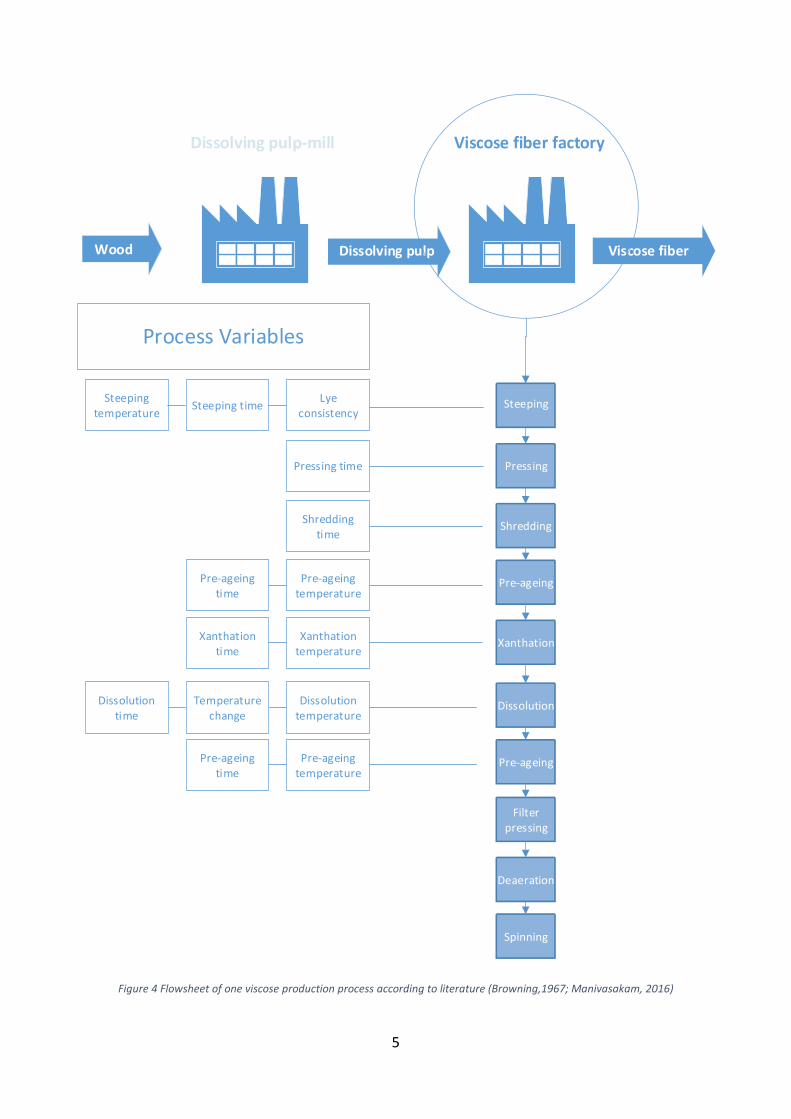
Viscose fiber production, also referred as cellulose xanthate process (Browning, 1967), consists of

multiple steps, and these steps are presented in a process flowsheet in Figure 4. Each step within

the process has variables that affect the runnability and quality of product. The process is well

studied and most of the variables have set values that assure runnability (Browning, 1967).

Dissolving pulp-mill

Wood Dissolving pulp

Viscose fiber factory

Viscose fiberWholeProcess

Manufacturing methods

Dissolving pulp properties

Process variables

Wood species

FactorsAffectingQuality

5

Figure 4 Flowsheet of one viscose production process according to literature (Browning,1967; Manivasakam, 2016)

Dissolving pulp-mill

Wood Dissolving pulp

Viscose fiber factory

Viscose fiber

Lye consistency

Shredding

Pre-ageing

Xanthation

Dissolution

Pre-ageing

Filter pressing

Deaeration

Spinning

Steeping

Pre-ageing temperature

Dissolution temperature

Temperature change

Pre-ageing temperature

Pre-ageing time

Pre-ageing time

Dissolution time

Xanthation temperature

Xanthation time

Process Variables

Steeping timeSteeping

temperature

Shredding time

PressingPressing time

6

2.2 Dissolving pulp

Dissolving pulp can be considered as more demanding pulp compared to traditional pulp used for

papermaking, when it comes to quality requirements. According to Jensen (1977), the anomalous

requirements compared to traditional pulp are higher chemical and physical purity, more uniform

quality and better reactivity. Therefore, the dissolving pulp is produced in different fashion to

traditional pulp, and the main differences exist in pulping and bleaching. Like traditional pulp,

dissolving pulp acts as an intermediate product and needs to be further processed. There are

multiple products that have been produced out of dissolving pulp. Some examples of these include

cellulose xanthate, which is further processed into viscose fiber, and cellulose nitrate, which is used

in explosives. (Jensen, 1977)

Molecular level events hold a vital role when it comes to refining pulp. The better those events can

be measured and presented, the better the behaviour during the refining process can be estimated.

In a perfect scenario all the molecular level events such as molecule distribution and molecular

structures are measured. In reality, the measurements are made to be simple and they often just

reflect those properties. Because the scenario is not perfect, the possible errors in estimations

needs to be considered. (Sjöderhjelm, 1999)

For this study the total number of properties measured to be used for the model is initially limited

to 32. All those properties are listed in Appendix 1. The measurements represent the behaviour of

the pulp. Even though it could seem that accuracy of the estimated behaviour rises when the

number of measured properties rises, it is not always true. With increasing number of

measurements within samples, the inaccuracy due random correlations increase as well. This

means, that these not contributing properties might seem to have an impact on the behaviour when

in reality the correlation can be a random incident. It is important to recognize this when

constructing a data driven model. Therefore, it can be an upside to have fewer initial measurements

rather that a lot. (Frenay, 2014)

7

2.3 Quality characterisation

There are two common properties that reflect the quality of a dissolving pulp and thereafter viscose

dope and viscose fiber. The properties are reactivity and filterability (Söderhjelm, 1999). According

to Strunk (2012), reactivity can be defined in multiple manners, and in the case of dissolving pulp it

can be called as accessibility as well. Regardless of multiple definitions, a broad idea of the reactivity

can be defined as a tendency of the cellulose to create cellulose derivates, and it is presented as a

percentage of residual cellulose or cellulose yield (Strunk, 2012). Filterability tests are done for

viscose dope (Browning, 1967; Strunk, 2012), and the test determines, how much viscose dope in

grams is filtered during two different time spans. The value is calculated and often corrected with

viscosity, making the resulting value unitless.

The commonly used measurement for reactivity is suggested by Fock (Strunk, 2012; Fock, 1959)

whereas the common measurement for filterability is suggested by Treiber (Browning, 1967;

Treiber, 1962). The procedure for both tests differs and both have their ups and downs. Fock’s test

is considered fast compared to Treiber’s test, but it lacks in precision. This is due to Fock’s test having

only single step in which the reactivity of the dissolving pulp is measured, whereas Treiber’s test is

based on replicating whole manufacturing process from dissolving pulp to viscose fiber, hence

having multiple steps. Fock’s test is designed for laboratory scale whereas Treiber’s test tries to

replicate a larger scale production and therefore operates in a bigger scale. This leads for a time-

consuming measurement procedure for Treiber’s test. Given the complexity of the Treiber’s test

combined with its superior precision, the data received from Treiber’s test is considered more

valuable than those received from Fock’s test (Jensen, 1977). This study is based on results received

only from Treiber’s test and therefore Fock’s test is not further discussed.

Treiber’s test results in a filtration value kw. The filtration value is calculated according to Equations

1 and 2. In Equation 1, t1 and t2 are filtration times and M1 and M2 are amounts of viscose dope in

grams filtered during the respective times. As an example of the filtration times, Strunk et al. (2011)

used filtration times 0-20 min for t1 and 0-60 min for t2. The initial filtration value is usually corrected

according to Equation 2, where η stands for the ball fall time in seconds for a standard viscose dope

viscosity analysis, resulting in a corrected filtration value Kw. (Strunk, 2011)

8

𝑘𝑤 = 2 ∗ [

𝑡2

𝑀2−

𝑡1

𝑀1] ∗ 105

𝑡2 − 𝑡1

𝐾𝑤 = 𝑘𝑤

𝜂0.4

Besides the fact that Kw is dependent on the filtration time and viscosity, different filters affects the

outcome as well (Strunk, 2011). In addition, different manufacturers use slightly different values for

the constants in the calculation equations, and therefore received Kw values cannot be compared

by default between different manufacturers or laboratories. Even though exact Kw values are not

comparable, the relative values can be compared to certain extend with one common rule: the

smaller the Kw value, the better the quality of the product for further processing. A flowsheet for

Treiber’s test is presented in Figure 5. The flowsheet has similarities to the one presented in Figure

4, but only measured properties that are included in the available data are presented. (Browning,

1967; Treiber, 1962)

Treiber’s test can be considered the most accurate testing method due to its large-scale nature, but

it is worth mentioning that it is by no means a default procedure that is available at every factory or

even for every producer. Data for this study consists of just below 400 laboratory test samples, each

sample consisting of multiple measurements.

(1)

(2)

9

Figure 5 Flowsheet of the Treiber test with comparison to viscose fiber production (Browning, 1967; Treiber, 1962)

10

2.4 Modelling the viscose fiber quality

Viscose production has not been successful when it comes to modelling the process. So far, the

manufacturers have been running the process according to what has been done before and what

has been working out so far. The dissolving pulp grades that have been used are based on their

observed processability. The so-called rule of thumb philosophy has been widely used in forest

industry due to nonlinear behaviour of processes as well as large demand of the product. Quality of

the product has not been a crucial factor. Being able to get product, no matter what quality, out of

the factory has been the main goal. (Jensen, 1977; Sjöderhjelm, 1999) Nowadays the technology for

nonlinear modelling exists and is available for almost everyone. Estimations for even the most

chaotic processes can be presented with knowledge and, more importantly, with available data of

the process. (Mamitsuka, 2018)

11

3 Machine learning

Modelling with machine learning algorithms can be considered as data driven modelling. The idea

is to find a model that fits into the available data. The data is required to have one to n-number of

input features, and for a predictive model, one or more output features. The model itself either

calculates or estimates a response of inputs for a single output or for multiple outputs. For

traditional models, the model can be describeds as a function f(x1,x2,…,xn) where number of

variables depends on number of inputs, but for machine learning models there is not a single

function or a set of functions that describes the model. A machine learning model can be defined as

a program that requires a set of learning data from which it creates conclusions and dependences

between input and output features (Zhang, 2012).

3.1 History and usage

The idea of machine learning dates to 1970s to 80s (Mamitsuka, 2018), but the idea has gained more

attention as a subject for studies from the early 2000s. (Biau, 2012; Zhang, 2012) Machine learning

models have seen increasing numbers in usage, and they have been utilized for example in

biotechnology with DNA modelling (Antikainen, 2018) and modelling spontaneous combustion of

coal (Lei, 2018). Other recent studies related to both chemistry and machine learning include

reaction performance prediction (Ahneman, 2018) as well as machine learning models considering

molecular behaviour (Wu, 2018). No reports of applications for forest industry were found. Either a

very little or no study at all has been done, or all the research on the topic considering forest industry

is confidential and not available for public.

12

3.2 Machine learning utilization

Machine learning is a powerful concept, and some of the basic algorithms are available for anyone.

Machine learning algorithms are included in calculation and modelling softwares with paid

subscriptions, such as MATLAB (MathWorks, 2016), but there are also some open source algorithm

libraries for different programming languages, such as Sklearn for Python (Pedragosa, 2010).

Utilization of machine learning is covered in next sections.

3.2.1 Approach

A lot of things are to be considered and there are many requirements to justify the usage of machine

learning and choosing a correct algorithm. The decision process can be broken down into two key

questions. The first question is, should a supervised or unsupervised learning be utilized. When

unsupervised approach is chosen, no further major deciding questions remain, but for supervised

learning the problem can be broken down even further. It needs to be decided, whether the model

should be a classification model or regression model. Figure 6. illustrates the simplified decision

path for the machine learning approach. (Mamitsuka, 2018; MathWorks, 2016)

Figure 6 Simplified decision path for machine learning approach (MathWorks, 2016)

13

There are clear guidelines for deciding between supervised and unsupervised learning. For a model

that is expected to be a predictive model that results with a response, a supervise approach should

be used, whereas for model that is used to gather more information of the data and to find

dependencies inside the data, an unsupervised approach should be utilized. The main difference for

these two approaches is, that supervised learning requires a response feature whereas

unsupervised learning does not. Furthermore, the guidelines for the decision between regression

and classification model are clear as well. If the expected outcome should be a continuous number,

a regression model should be chosen, whereas if the outcome is expected to be discrete, a

classification model should be chosen. (Mamitsuka, 2018; MathWorks, 2016)

Machine learning always depends on data. Besides deciding the outcome of the model,

understanding the utilized data type affects the decision of the algorithm. Data types include

numeric data as well as texts and images. The data types are considered more in depth in the

Chapter 3.2.2. (Mamitsuka, 2018)

For certain data types and expected outcomes there are usually several machine learning algorithms

available, and they are often like each other with minor optimization differences. It might not be

possible to decide the correct algorithm solely based on written theory, and according to

MathWorks (2016), the model selection often comes down to trial and error.

Deciding the right algorithm to be utilized is a large part of the model building process. The following

steps depend on the algorithms used, but there are simplified guidelines for finishing the model.

The steps include pre-processing the data, deriving features, training the model and finally iterating

and optimizing the model. A simple workflow for machine learning model process is presented in

Figure 7. (MathWorks, 2016)

Figure 7 Workflow of a machine learning process according to MathWorks (2016)

14

The data is rarely ready to be utilized with machine learning algorithms, and therefore the data

needs to be pre-processed. Pre-processing includes filling missing data gaps with different data

generation methods as well as removing the data sets with clear measurement errors. (Pedragosa,

2010) Features and their selection is explained in the following section, as well as training the model.

3.2.2 Data types and algorithms

For machine learning algorithms, there are some terminology that needs to be explained. The data

consists of multiple instances, and the instances consists of multiple features. For supervised

learning it is also required, that each instance has a response feature. Considering dissolving pulp as

an example of a vector data type. Each individual dissolving pulp sample acts as an instance, and all

the measured properties and variables associated with that dissolving pulp are considered as

features. The result is a matrix, and therefore the data type is called vector. Table 1 illustrates the

matrix. (Mamitsuka, 2018)

Table 1 Matrix formed of instances and features. a-n/1-m represents numerical values

Feature 1 Feature 2 Feature 3 Feature 4 … Feature n

Instance 1 a1 b1 c1 d1 … n1

Instance 2 a2 b2 c2 d2 … n2

Instance 3 a3 b3 c3 d3 … n3

Instance 4 a4 b4 c4 d4 … n4

… … … … … … …

Instance m am bm cm dm … nm

15

Besides vector data type, Mamitsuka (2018) suggests that there are five other data types utilized by

machine learning algorithms: sets, sequences and strings, trees, graphs and nodes in graph. For each

data type there is a list of machine learning algorithms that can be associated with them. Table 2

illustrates algorithms and methods that should be used with each data type.

Table 2 Machine learning algorithms arranged according to data type they utilize (Mamistuka, 2018)

The complexity of the data type increases, when moved from left to right on the Table 2. When

moved to the right, each data type can be considered as a special case of the previous data types.

This explains the high number of algorithms associated with vector data type. When it comes to

choosing and eliminating algorithms to be used, it would be advantageous if the case could be

considered as a more complex data type. (Mimatsuka, 2018) Figure 8 illustrates the differences of

the data types.

Vectors Sets Sequences and strings Trees Graphs Nodes in a graph

Methods

*Clustering:

-Objectives

-K-means

-Constrained K-means

-Finite mixture model

-Hierarchial clustering

*Probaballistic model

*Matrix Factorization

*K-nearest Neighbors

*Decesion Stump

*Decision Tree

*Bayesian classifiers

*Linear Ridge

Regression

*Logistic Regression

*Layered neural

network and deep

learning

*Ensemble learning via

sampling

*Ensemble learning via

three hypotheses

*Ensemble learning:

AdaBoost

*Support vector

machine

*Frequent patter mining

-Apriori algorithm

-FP-growth algorithm

*Probaballistic model

*Kernel learning

*Frequent subsequence

mining

-Generalized sequential

patterns

-PrefixSpan

*Probaballistic models

for sequences

-Mixture Markov model

-Hidden Markov model

*Kernel learning

-Spectrum Kernel

-All subsequence Kernel

*Probaballistic models

-Hidden tree Markov

model

-Ordered tree Markov

model

*Kernel learning

-All subtree Kernel

*Frequent subtree

mining

*Frequent subgraph

mining

-gSpan algorithm

-Reverse search

*Kernel learning

*Spectral clustering

*Matrix factorization

*Label propagation

Data type

16

Figure 8 Data types associated with machine learning (Mimatsuka, 2018)

Vectors: Sets:

Feature 1 Feature 2 Feature 3 Feature 4 Instance 1: {A,B,C,D}

Instance 1 A B C D instance 2: {D,C,B,A}

Instance 2 A C C C

Instances, each being a vector, are a matrix Two instances, each being a set

Trees:

Sequences and strings:

Instance 1

Instance 1: DCBA

Instance 2: ADBCA

Two instances, each being a sequence

Instance 2

Two instances, each being a tree

Graphs:

Instance 1 Instance 2

Two Instances, each being a graph

A

D C

B

D

A B

C B

DA

D

D

B D A

B

A B

C

A

17

Vectors are the simplest data type of the six. For vectors, each instance has the same number of

features, but the features do not need to be in any specific order. For data that is not whole, the

instances with missing feature values require some data generation.

Sets are a special case of vectors. Number of features for each instance is not required to be the

same, and the features do not need to be in specific order. In the example presented in figure 8, the

two set instances are actually the same and considered identical, even though the features are in

different order.

Sequences and strings are a special case of sets. For these, the number of features is not restricted,

but the order is significant. These first three data types, vectors, sets and sequences, do not

consider, what the relationships between the features within each instance are. For the rest of the

data types, the relationship is significant.

The relationships for trees, graphs and nodes in graphs can be considered as routes. What differs

the trees and graphs is, that for trees there are only one route from one feature to other, whereas

for graphs there can be cyclic structures and therefore multiple routes. For nodes in a graph, there

was no illustration available by Mimatsuka. What is said about them is, that for them one instance

is a node in the graph. An example is given, where the world wide web is considered as a huge graph,

and homepages are the nodes. The important thing to understand about different data types is their

existence and relationship to modelling possibilities. (Mamitsuka, 2018)

When the data is known and inspected, and a machine learning algorithm is chosen, the final major

step for the model building is training the model. Each algorithm works in its own way, but basically

the algorithm takes the input data, usually referred as training data, and re-arranges and forms

conclusions and dependencies from it. The training part is the heaviest part in the machine learning

model’s building process, and for large models it can take a lot of time. Some algorithms are lighter

than others with a price of accuracy, which is a reasonable thing to discuss during the algorithm

selection. Trained model can either give structural information of the data (for the case of

unsupervised learning), or it can be given data and the model predicts the response (for the case of

supervised learning). Finally, the model can be fine-tuned with algorithm specific variables, but the

effect is marginal compared to difference between algorithms. (Mamitsuka, 2018; MathWorks,

2016)

18

3.3 Random Forest algorithm

3.3.1 Basic idea

Random Forest algorithm is one of the ensemble methods for machine learning, and it is basically a

data driven model. The Random Forest algorithm has two variations for two types of problems. The

first one answers classification problems and the second one answers regression problems. The

main idea remains the same for both variations. The Random Forest algorithm utilizes learning trees

and combines them, hence the name Random Forest. The whole modelling procedure consists of

two phases, a training phase and a predicting phase. (Zhang, 2012)

The learning phase requires data that consists of features and responses. The learning trees are

composed of so-called nodes, that basically acts as deciding points for the features. There are two

types of nodes, splitting nodes and terminal nodes. At each node it is checked, if the node can be

split according to certain rules. If splitting is not possible the resulting node is called terminal node.

It can be imagined, that the learning tree is a path and the nodes are crossroads within the path,

terminal node being the end of the path. The splitting nodes act in a binary partitioning fashion. For

classification problems the rule for each node is whether the feature in question belongs to a certain

group, whereas for the regression problems the node checks, whether the value of the feature is

bigger or smaller than a set value. When the last considered feature is split and the terminal node

is reached, the algorithm takes look at all the formed paths and sets all the responses of each path

for their corresponding terminal node. The terminal node is basically an average of all the responses

that fall into the terminal node in question. For regression problems each feature could have

multiple splitting nodes depending on the disparity of the feature. An example of a learning tree is

presented in Figure 9. (Biau, 2010; Zhang, 2012)

19

Figure 9 An example of a learning tree built for a regression model. X1 to X5 are features used and numbers at the bottom are the responses for each path constructed (Biau, 2010)

It is suggested, that not all the available features should be utilized at the same time. (Frenay, 2014)

This gives a possibility for multiple learning trees due to multiple possible combinations of features.

These random combinations of features and combinations of these gives valuable information of

the importance of each feature. It is also faster to form multiple smaller trees rather than one large

tree. It is found, that the number of trees utilized in the forest can be significantly smaller than the

number of available trees. If the data is consistent and feasible for the usage of the Random Forest

algorithm, the algorithm will always create a reasonable model for the response. This achieved

model is always a little different, not significantly though, and hence the prefix “random”. (Zhang,

2012)

20

Once the model has finished building, the predicting phase for the unknown data sets can begin.

The phase is straight forward. The data set is compared against all the learning trees within the

forest. Not using all the features during building the forest acts in our favour due to being able to

create multiple comparison trees of the single data set. The algorithm creates the same

combinations of features as were used during the building phase and checks the fitting responses

for the data set in question. If multiple comparison trees lead to the same response, the response

is most likely accurate, whereas if all the comparison trees lead to different result there is most likely

problems with either the tested data or the model itself. (Zhang, 2012)

3.3.2 Requirements and setup

Using Random Forest algorithm requires setting up. Amount of setup required depends on the

quality of data used for the model. If the data is consistent, for example all the samples are from

the same laboratory and each data point includes all the same measurements, only a little setup is

needed, whereas inconsistent data requires more attention. Setup manoeuvres include

consideration of missing data, normalization of data and feature selection.

A clear requirement for Random Forest, or any data driven model, is to have a sufficient amount of

data available. Calculations for the required sample size exists for linear regressions (Cohen, 1988),

and Shahinfar et al. (2018) suggests, that these calculations can be utilized to get the idea of the

sample size. For example, a calculated value to reach 95% power with 1% error yields in need of

over 2000 samples (Shahinfar, 2018; Cohen, 1988). This means, that a sufficient number of samples

needs to be in thousands rather than in hundreds, which is the case for a number of the published

machine learning studies (Sette, 2004; Ahneman, 2018; Antikainen, 2018; Lei, 2018; Shahinfar,

2018; Wu, 2018). Exceptions exists, and for example a study by Lei et al. (2018) got reasonable

results with a Random Forest model with only 220 samples.

In theory data is not required to be whole for Random Forest (Zhang, 2012). This is due to the

Random Forest algorithm being able to calculate so called proximities for the learning data. The

proximities are calculated during the construction phase and they basically consider, how similar

samples are compared to each other. To be able to construct the model, the missing values needs

to be filled initially by setting their values to be median values of the properties in consideration.

21

Samples with initially guessed data are compared to similar samples with complete data, and based

on those similar samples, a new value is calculated for the missing data. A well coded Random

Forest algorithm would iterate the building process multiple times to find the most stable

imputations for missing data, but if open source programming library, such as Sklearn is used, a

nominal data generation is required. (Pedregosa, 2010) This means that the algorithm cannot

process the data if blank spaces remains, and the algorithm is not coded to do the iteration process.

The redeeming factor is that error due to data generation diminishes due to building multiple

random learning trees from the data. (Zhang, 2012)

Besides data being nominally complete, the data needs to be normalized. This means that all the

features should be put into the same scale for example between -1 to 1. By normalizing the data,

the algorithm recognizes relative differences within the features. (Pedregosa, 2010)

Feature selection is suggested to be completed to achieve the final model. (Frenay, 2014) The

algorithm can calculate the feature importance, which is based on the random feature combinations

that the algorithm creates itself. (Pedregosa, 2010) It evaluates, which features has the most to do

with the response by checking, which features do have a little to no effect when left out of the

learning tree. The feature selection is not a necessity for the function of the model, but it saves a lot

of computing power and time when the number of learning data is increased. (Frenay, 2014;

Pedregosa, 2010)

Studies considering Random Forest approach such as Abellán et al. (2017) studying Random Forest

approach using imprecise probabilities, Antikainen (2018) studying protein-DNA binding specificities

modelling with Random Forest and Lei et al. (2018) studying Random Forest approach for predicting

coal spontaneous combustion have not considered the setup procedures to the detail. All the above-

mentioned studies state, that they have utilized precise data, suggesting that no data generation

was required. For these studies, the approach seems straight forward. Data has been ready-to-use,

and only parameters that were considered were the size of the forest and number of maximum

features. These parameters as well as other tuneable parameters according to Pedragosa (2010) are

presented in Table 3.

22

Table 3 Tuneable parameters for Random Forest algorithm (Pedragosa, 2010)

Parameter Explanation

Number of trees in forest Total number of trees build during training. Default number is ten.

Maximum depth Defines how deep the trees are. Default depth continues the building until samples cannot be split anymore.

Minimum samples split The minimum number of feature samples remaining required for the node to split. Default number is two.

Minimum samples leaf The minimum number of feature samples that would appear in the next node. Default is one.

Maximum features The number of features used for each individual tree built. Default is the number of features available.

Besides no mentions of data generation, data scaling and -normalization are not considered in the

studies either. Zhang (2012) and Pedragosa (2010) suggests that normalization and scaling are

important factors, so the procedures could be self-evident, and therefore they are not mentioned.

3.3.3 Scoring the model

A so called out-of-bag (OOB) -score can be calculated for the Random Forest model by leaving some

of the data points that would be used for fitting outside the fitting procedure. These data points are

used instead as testing points for the model. The OOB-score tells, how well the unknown points can

be predicted with the model. (Pedregosa, 2010)

23

Removing some amount of data in order to verify the functioning of the model raises question of

how it is decided which data is to be removed. For models with low number of data points, removing

multiple data points at time could make a big difference. To avoid any questionable removal system,

such as the researcher choosing the removed samples in order to manipulate the results, a simple

script is utilized for pure OOB prediction. The script takes the input data table and removes the first

sample from it. Then a model is built with the data that lacks the removed sample. Then a prediction

is made for the one sample that was removed. Finally, the removed sample is added back to the

data, to the last place in the data table. The procedure is repeated until each of the sample has been

handled. This way each sample within the data can be considered as true OOB-sample due to not

being included in the training data, and at the same time the number of training data is kept at the

highest possible. (Pedregosa, 2010)

24

Applied part

4 Materials and methods

Data used is received from SciTech-Service, which is a consulting company that has expertise in

dissolving pulp industry. The data consists of Treiber-test results of dissolving pulps as well as

measured properties of dissolving pulp utilized and some process properties. List of all the

measurements included is listed in Appendix 1. The Treiber-test data is received from Säteri-mill

and the data consists of measurement-data of dissolving pulp from different mills from a timespan

of over ten years. For the sake of clearance, data received from one test routine is called a data

point in this study. Initially, the total number of data points is 500. Due to different test routines in

mills, the data is not whole. A manual check was done for the data points and only data points with

each process variable available were kept. Also, data from two mills was initially excluded due to

the pulps being from time during the start-up of the mills. During mill start-up, the process can be

unstable, and this could have an unknown impact on the dissolving pulps, therefore possibly

affecting the model. This leads to usage of just a little under 400 data points, more exactly 370 data

points. Figure 10 illustrates the relative amounts of pulps from different mills.

Figure 10 Relative amounts of pulps from different manufacturers

25

There are two serious problems with available data that need to be considered. The first problem is

validation of the data. Measurement errors could exist, as well as data that has been prepared from

failed tests. Most common validation method is to do parallel tests of the same sample to point out

the errors, but for the data utilized for this study this has not been done. It is with high importance

to isolate the uncertain data points from the data that is used for teaching the model.

The second problem is missing data within data points. Not every data point has all measurements

included. This is due to differences between dissolving pulp mills. Pulps from the same mill have the

same measurements, but comparison between different mills creates these holes.

Considering the two problems, there are two ways to study the applicability of machine learning for

the quality characterisation. The first way is to try and utilize all the data for the model and find a

“universal” model, a model that could predict the response for any pulp grade. This requires data

generation for missing measurements within data points, and an assumption, that all the necessary

measurements are done. This means that for example all the machinery between different mills is

expected to not have an effect for the outcome. There seems to be multiple factors that could go

wrong. This leads to consideration of the second approach, which aims to minimize all these factors.

The approach is constructing mill specific models. For these models the only obvious downside is

the number of data points in the learning data being small. Besides that, no data generation is

required, and number of unknown factors, such as differences between machinery, can be

reasonably assumed to be low. For the mill specific models, a model was built for pulp grades one

to five from the Figure 10 due to reasonable amount of data points available, as well as for one of

the two excluded pulp grade that was mentioned in the beginning of the Chapter 4. Inspection of

the excluded pulp grade is due curiosity and due to the fact, that it has as large number of data

points available. Even though the start-up phase can be expected to be unstable and the quality

being poor, the environment has been the same for all the samples.

As mentioned in Chapter 3.2.1, model creation consists of multiple steps. Figure 11 illustrates the

steps included for the model creation in this project. The steps are basically the same as suggested

in Chapter 3.2.1, with addition of breaking some steps into sub steps. The steps are considered in

following subsections 4.2-4.6. for both, the universal model and mill specific models.

26

Figure 11 Steps included for model creation

4.1 Algorithm selection and justification

An initial feature analysis was done prior to this study by GloCell and SciTech Service. The analysis

was a Principal Component Analysis (PCA), and it suggested that correlations exists within the

data, but this information could not be utilized any further. That initiated this study to go deeper

into the feature dependences. The significant outcome of the PCA is, that the data does not seem

to be absolutely random. There are traces of correlations, in which the machine learning

algorithms lean on.

As mentioned in chapter 3.1, no studies considering machine learning associated with forest

industry were found. Therefore, applying the machine learning philosophy needed to be started

from blank. As suggested in the chapter 3.1, the suitable algorithm can be found with assistance of

literature as well as with a trial and error method. MATLAB includes many machine learning tools

to work with and they were utilized to get the idea of whether the application is reasonable and

what sort of model could be applied. Initial trial and error attempts deduced that machine learning

model Random Forest could be reasonably applied for the study.

27

As mentioned in Chapter 3.2.2, information of the data type utilized can be used as an assisting tool

for choosing a suitable algorithm. For this case, the data type is clearly a vector, due to the data

consisting of multiple instances, which are constructed of the same exact features. This limits the

number of the algorithms a little. The Random Forest algorithm suggested by trial-and-error method

belongs in to the ensemble learning methods, which is a suggested method for vectors in the Table

2.

The data utilized for this study has structure for machine learning algorithms, and the data has a

supported data type for multiple possible machine learning algorithms. Trial-and-error approach

suggests the Random Forest algorithm, which has been utilized in studies with close to similar data.

With this information it can be concluded, that utilizing Random Forest algorithm is the most

feasible approach to study the machine learning applicability for viscose quality characterisation.

The emphasis of this study lies more in the utilization of the Random Forest algorithm rather than

studying the algorithm itself, and therefore an existing Random Forest code is utilized. The code

libraries are from open source collection for Python called Sklearn (Pedergosa, 2010), and no

modifications has been made for the algorithm code.

4.2 Handling missing values

As discussed in previous section, the data for the universal model is not whole, and this needs to be

addressed. For mill specific models, no data generation is required.

To get the most out of the available data, the missing data needs to be generated. For this case

there is no strictly superior method, because the data and measurements could be much dependent

on the mill environment rather than the process. Nevertheless, there are three different approaches

to make the data whole. (Pedregosa, 2010) Each method utilizes all the available data and generate

the missing values in three diverse ways. The ways are most frequent value, mean value and median

value. The most frequent value approach gives each missing value the most frequent value of each

feature whereas the mean and median values calculates the mean and median values for each

feature and uses it for the missing points. No significant difference was noticed between these three

methods, so median approach is used.

28

4.3 Initial model

The initial model is constructed with the 370 data points that were decided in the Chapter 4. The

results of the initial model give an idea of the precision that could be achieved with the available

data, as well as gives hints of possible uncertain data points. Ideally the data includes parallel

measurements, which reduces the possibility of measurement errors and hence possibility of invalid

data drastically.

For this case the starting point is weak when the above-mentioned factors are considered. It is

unknown, which data point are invalid, and almost every data point is missing one or more

measurement. Additionally, no parallel measurements are included in the data.

The initial model was constructed with Python, and Sklearn libraries (Pedragosa, 2010) were utilized.

The libraries included “Imputer”, “StandardScaler” and “RandomForestRegressor”. Imputer library

was used to generate missing values and StandardScaler library was used to scale and normalize the

initial data point values to values between -1 to 1 so that the machine learning algorithm can

manage the data. RandomForestRegressor library is the Random Forest algorithm itself. Initially all

other parameters for all the functions remained untouched, but for the RandomForestRegressor,

the number of trees built was set to 500, due to default value of 10 is too low to get feasible results

(Zhang, 2012).

Besides the libraries concerning the machine learning, a library collection called Pandas was used

for data- and file management. Pandas libraries allows extraction of data from Excel file to be used

in the Python program, and ultimately the Pandas libraries allows creation of an Excel file from the

data in the Python program. (McKinney, 2011)

The precision is not expected to be high for the initial model, and this is seen in the results. Figures

12 and 13 illustrate the prediction precision for the OOB predictions and Figures 14 and 15 illustrates

OOB predictions against measured values.

As mentioned in Chapter 2.3, a lower Kw value means higher quality. For this case, a Kw value below

10 is considered good, Kw values between 10 and 20 are reasonable and Kw values above 20 are

bad. Therefore, throughout this study the behaviour at the region of Kw values below 20 is

considered more closely.

29

Figure 12 Prediction precision for predicted Kw values below 20 and all the predicted Kw values of the universal model

Figure 13 Prediction precision for predicted Kw values below 20 and all the predicted Kw values of mill specific models combined

sFor the mill specific models, the precision is a little more promising for Kw values below 20, but still

far from good. As it can be seen in Figures 12 and 13, the precision of the universal mode increases

clearly when error rate increases, whereas for the mill specific models the precision is far smoother.

It is evident, that a model with error rate of +/- 1 with decent precision is out of reach, but a model

with lesser than +/- 10 error rate with good precision could be achieved.

0%

10%

20%

30%

40%

50%

60%

70%

80%

90%

100%

+/- 1

+/- 2

+/- 3

+/- 4

+/- 5

+/- 6

+/- 7

+/- 8

+/- 9

+/- 10

Prediction precision - Universal Model

Kw < 20

All Kw

0%

10%

20%

30%

40%

50%

60%

70%

80%

90%

100%

+/-1

+/-2

+/-3

+/-4

+/-5

+/-6

+/-7

+/-8

+/-9

+/-10

Prediction precision - Mill specific models

Kw < 20

Kw All

30

In Figures 14 and 15, there is a slight, but noticeable trend able to be seen, but also many outliers.

Especially the mill specific models exhibit a linear behaviour between predicted and measured

values. There are many outliers in the region between predicted Kw values 10 and 20. This suggests,

that learning data could include uncertain data points. The uncertain data is considered more in

depth in Chapter 4.6.

0

10

20

30

40

50

0 10 20 30 40 50

Mea

sure

d K

w

Predicted Kw

0

5

10

15

20

0 5 10 15 20

Mea

sure

d K

w

Predicted Kw

Universal model

0

50

100

150

200

0 50 100 150 200

Mea

sure

d K

w

Predicted Kw

0

5

10

15

20

0 5 10 15 20

Mea

sure

d K

w

Predicted Kw

Mill Specific Models

Figure 14 Measured Kw against predicted Kw for the universal model

Figure 15 Measured Kw against predicted Kw for the mill specific models combined

31

4.4 Feature selection

For building a Random Forest model, available data has one restriction. The data needs to be

considered as input-output dependency, where measured properties and other variables form a

group of input features and one property acts as a response feature. In this case, all the

measurements listed in Appendix 1 act as features and filtration value Kw acts as response.

There are a lot of measurements included in the data. Not all the different measurements can or

should be used for the model. Not all the features influence the result, and some features might

have a false effect, dragging the model into wrong direction. It is required to reduce the number of

features to reach a more stable model. (Frenay, 2014) The feature selection can be done in

assistance with certain algorithms. (Pedragosa, 2010)

Random Forest algorithm used for the model building holds within its building process the feature

analysis output as well. (Pedragosa, 2010) The algorithm does the feature selection basing on the

feature importance it calculates. The feature importance needs to be checked by hand to find out,

whether only one feature overpowers the whole model, or if the feature importance has an even

spread. Brief explanation for each feature is given in Appendix 1. Figures 16 and 17 illustrates the

feature importance for the models under development. For the universal model It suggests, that

one feature, S18, holds a significant role for the model, but is not overpowering the model too much.

For the mill specific models, the process variables seem to hold the most significance. The difference

comes from the nature of the data. Mill specific data has consistent and similar values for pulp

properties, and the largest differences that affect the filterability comes from process variables. For

the universal model, pulp properties seem to affect the outcome more than the process variables.

It is worthy to consider the least noteworthy features and why the Random Forest algorithm

suggests them to have no impact. Most of the least impactful features for all the models consists of

different wood species. Besides wood species, bleaching and cooking method appear to have close

to no impact. The common factor for these features is, that the effect of these features could be

seen in other measures. Using certain cooking or bleaching method or utilizing certain wood species

could be reflected in other features, therefore making the existence of wood species and those two

methods in model insignificant.

32

Feature Importance - Mill specific models

Feature Importance - Universal model

Figure 16 Relative feature importance of the universal model

Figure 17 Relative feature importance of the mill specific models

33

4.5 Data composition

There are 370 points of measured data available for the modelling of the universal model. The data

is not from a single factory or producer, but from a broad scope of 22 different manufacturers. The

data composition according to manufacturers is presented in Figure 18. It should be noted, that one

manufacturer represents almost one third of the whole data.

Figure 18 Initial composition of pulps according to different manufacturers

Random Forest algorithm is more accurate, when more data is available. (Frenay, 2014) What is

more important, is how the data is spread throughout the responses. As mentioned in Chapter 3.3.2,

370 data points is a rather small number of data points for a Random Forest algorithm, meaning

that a more precise inspection on the data composition should be considered. The initial data

composition according to Kw value is presented in Figure 19a. The composition is far from being

equally spread or balanced. Most of the data points are at Kw range between zero and twenty. For

the model this means, that behaviour at the lower end is more precisely learned whereas at the

higher end the behaviour is not well learned. This can be seen in the prediction precision, that was

considered in Chapter 4.3. Lower end is more precise than higher end.

34

Figure 19a Initial spread of measured Kw values Figure 19b Categorized Kw spread of measured Kw values

The data composition needs to be addressed. The problem as it is in this case does not exist in most

of the learning algorithm cases where the number of learning data is in thousands. Especially for

this case, no specific study plan has been made to study exactly the data behaviour with Random

Forest algorithms, but rather the data consist of samples received from production phases at the

mills. Therefore, there is no universal solution for the problem. For this case the problem could be

eased by creating a classification problem first, rather than a straight forward value prediction

problem. The suggestion is as follows. The model is a twofold system that first gives both a

categorized prediction and a more precise, numerical prediction. Categorized response spread

where the split point value for Kw is 10 is presented in Figure 19b. Split point means the value that

divides the responses into categories. With split point value 10, first response category consists of

Kw values below 10 and the second response category consists of Kw values above or equal to 10.

020406080

100120140160180

0-10 10 to20

20 to30

30 to40

40 to50

50+

NU

mb

er o

f d

ata

po

ints

Measured Kw

Initial measured Kw spread

0

50

100

150

200

250

0-10 10+

Nu

mb

er o

f d

ata

po

ints

Measured Kw

Categorized measured Kw spread

35

4.6 Uncertain training data

The most important thing when dealing with such a small number of training data is to find the

uncertain data. That includes data that has had measurement error or unknown situational error.

Finding the uncertain data point can be really challenging and needs to be done with caution. There

is no simple tool to find incorrect data, but for this case it can be done by hand due to low number

of data points. A number of methods is suggested by Frenay (2014) and one of them can be utilized

for this case.

The method used for finding and removing uncertain data is basically training the model and

removing those training data point, that does not give desired feedback. This is done by comparing

data points and trying to find ones with similar features but different response.

4.6.1 Finding uncertain data

The good thing for such small data set is, that the inspection can be done manually with a little

assistance of scripted algorithms. The simple algorithm was coded for finding data points with

similar features. The similarity is decided with a threshold level, and the removal process is started

with small threshold level to find data points with almost exactly similar features. The data points

with similar features were thereafter compared manually to find data points with noticeably

different response values. In the case of only two or three data points with similar features, due to

not being able to decide which of the data points were wrong and which right, all of them are

removed. When more than three data points with similar features are present, the mismatching

path can be deducted and removed.

The initial removal process aims to remove all the data that is not good enought. A great portion of

data is removed in this case, leaving below half of the data (146 data points out of 370) for the

model. This is way too small number for a trustworthy model and it is irrational to suggest that over

half of the data cannot be used. The initial step is bound to remove good data as well, and therefore

a second step, which is based on the model feedback, is performed.

36

For the second step, all the available data is predicted with the models, universal and mill specific,

that are constructed of the 146 data points. This is done to find data points that are not included in

the model and the model can predict with reasonable certainty. In other words, the model

constructed of the most certain data is used to find out, which of the removed data points match

the behaviour of the model. Thereafter, the points that had not been included in the model that can

be predicted well are included in the training data. This results in a much higher number of training

data and therefore a much more versatile model. This type of data validation could be used as well

for further improvement of the model when more data becomes available.

The most obvious danger in doing a feedback-based data addition into the training dataset is, that

the initial dataset could be consisted of bad data and therefore the feedback learning results in a

model that seems to be behaving well with the data, but in the reality the model has been over

fitted with incorrect data. In this case it has been made sure, that the data used is consistent and

good by including only data points, that show similar behaviour with each other. The hypothesis is

that if more than three data points with similar features results in similar response, the data points

are good, and if a data point does not have similar data points in the available data, the data point

is considered incorrect. Therefore, the feedback step explains the behaviour of the single pulps that

have been removed.

4.6.2 Data composition after removing uncertain data

The removal process for the uncertain data is a crucial part of the Random Forest model building

and it can cause some troubles if it is done in wrong fashion. It is important to analyse the data that

has been removed as well as the data that remains. For the data that remains the analysis that can

be done is by looking at the composition of data, its manufacturer spread as well as response spread.

If the manufacturer spread has gone more uneven or if only a small scope of response is remaining,

the removal process has not worked out and the data removed is not actually bad, rather the model

is built for a small scope of data instead.

The removal phase consisted of two steps. Initial step resulted in 146 data points remaining. The

data composition and response spread of the 146 data points are presented in Figures 20a and 20b.

The manufacturer spread has remained good, and the response shows a slight change.

37

Figure 20a Manufacturer spread of pulps after first removal Figure 20b Kw spread after first removal

The second step in the removal process is the addition of data through a feedback step. The addition

step resulted in total of 258 data points in the training data. The data composition and response

spread of the 258 data points are presented in Figures 21a and 21b. The manufacturer spread and

the response spread have remained good, which suggests a balanced model when it comes to data

usage.

Figure 21a Manufacturer spread of pulps after addition Figure 21b Kw spread after addition

0

10

20

30

40

50

60

70

80

90

0-10 10+

Nu

mb

er o

f d

ata

po

ints

Measured Kw

Measured Kw spread

0

20

40

60

80

100

120

140

160

0-10 10+

Nu

mb

er o

f d

ata

po

ints

Measured Kw

Final measured Kw spread

38

4.7 Parameter optimization

Random Forest algorithm can be fine-tuned with certain parameters. The reason for fine-tuning of

the Random Forest model is not that much because of optimizing performance, but rather

improving computing efficiency. All the parameters that can be tuned for the Sklearn’s Random

Forest algorithm are presented in Table 4. Most of the parameters are used with their default values,

but two of them were modified for this study. Those parameters are the number of trees in the

forest and maximum features used for each tree. (Pedragosa, 2010)

Table 4 Parameters that can be tuned for Random Forest algorithm

Parameter Explanation

Number of trees in forest Total number of trees build during training. Default number is ten.

Maximum depth Defines how deep the trees are. Default depth continues the building until samples cannot be split anymore.

Minimum samples split The minimum number of feature samples remaining required for the node to split. Default number is two.

Minimum samples leaf The minimum number of feature samples that would appear in the next node. Default is one.

Maximum features The number of features used for each individual tree built. Default is the number of features available.

39

Prior studies of Random Forest were used as an assistance for the parameter tuning in this study.

(Abellán, 2017; Biau, 2010; Frenay, 2014; Zhang, 2012) This is due to the change of parameters

showing as more consistent goodness in results rather than improvements in individual goodness

of tests. For number of trees in forest it is suggested, that after a certain point the increasement

does not seem to affect the model behaviour anymore. The number of trees is bounded to the

number of the data sets, and therefore the number of trees required is case-specific. As Figure 22

illustrates, the error rate diminishing fades off rather quickly. (Zhang, 2012) For this study, 500 trees

were found to be good enough number to give consistently satisfactory results.

Figure 22 Out-of-bag error diminishing with increasing number of trees built for the Random Forest (Zhang, 2012)

Maximum number of features used has multiple possibilities, ranging from squared number of total

features all the way to near the number of total features. This parameter is case-specific as well,

and possible number of features was tried out between the given scale. (Pedragosa, 2010) The

number ended up with is 0.7 in range where 0 is no features and 1 is all the features.

40

4.8 Information of the model

Data handling was fully coded with Python. Outside libraries used for the model include Pandas-

library (McKinney, 2011) for transferring data from excel, and Sklearn-library (Pedragosa, 2010) for

the Random Forest algorithms. For the demo program PyQt5-library was used to create a graphical

user interface. Due to non-disclosure agreement, the source code is not presented.

The main application for the model is to predict a value for filtration value Kw with the given

properties. Input for the model is in form of Excel file with a determined format. The first row must

consist of the names of the properties in the correct order. Below the properties row comes all the

individual tests that are to be predicted, each for their own row. Not all the properties need to be

filled to be able to get a prediction. For the most accurate result, the more there are properties, the

better. The demo program is very simple and is just to demonstrate and test the functioning of the

model. It asks for Excel file with to be predicted data point and thereafter calculates the predictions.

The result is an Excel file that include the predicted value of filtration values as well as list of all the

similar data point for each data point in the initial excel file. The graphical interface of the demo

program is presented in Figure 23.

Figure 23 Graphical interface of the demo program

41

5 Results

5.1 Model behaviour and model precision

Total number of models constructed in this study is twelve: both classification and regression

models for universal model and five mill specific models for mills with reasonable amount of data

available. For machine learning models, the model behaviour is to be done with out-of-bag (OOB)

samples. The idea is presented in Chapter 3.3.3.

The OOB-predictions are considered the most reliable indicators of the functioning of a machine

learning model. The OOB-predictions were made for each of models constructed in this study, and

the results are illustrated in Figures 24-27. Figures 24a and 24b represent the prediction precisions

and Figures 25-26 illustrates the comparison between measured Kw values and predicted Kw values.

For the classification models the responses were divided into two: above and below 15. For universal

model, the OOB-precision of the classifying model is 0.86, meaning that 86% of the data points could

have been predicted correctly to be below or above 15.

The initially excluded pulp was noticed to behave well, and therefore it was ultimately added into

the universal model. It does not affect the model behaviour much, as Figure 27 illustrates, but it

affects the classification model drastically. The OOB-precision of the classifying model predicting

whether the response is below or above 15 got up to 0.95.

Figure 24a Prediction precision for predicted Kw values below 20 Figure 24b Prediction precision for predicted Kw values below and all the predicted Kw values of the universal model 20 and all the predicted Kw values of the mill specific models combined

0%

20%

40%

60%

80%

100%

+/- 1

+/- 2

+/- 3

+/- 4

+/- 5

+/- 6

+/- 7

+/- 8

+/- 9

+/- 10

Prediction precision - Universal Model

Kw < 20

All Kw

0%

20%

40%

60%

80%

100%

+/- 1

+/- 2

+/- 3

+/- 4

+/- 5

+/- 6

+/- 7

+/- 8

+/- 9

+/- 10

Prediction Precision - Mill specific Models

Kw < 20

All Kw

42

0

50

100

150

200

0 50 100 150 200

Mea

sure

d K

w

Predicted Kw

0

5

10

15

20

0 5 10 15 20

Mea

sure

d K

w

Predicted Kw

Universal model with initially excluded pulp

0

10

20

30

40

50

0 10 20 30 40 50

Mea

sure

d K

w

Predicted Kw

0

5

10

15

20

0 5 10 15 20

Mea

sure

d K

w

Predicted Kw

Universal model without excluded pulp

0

50

100

150

200

0 50 100 150 200

Mea

sure

d K

w

Predicted Kw

0

5

10

15

20

0 5 10 15 20

Mea

sure

d K

w

Predicted Kw

Mill specific models combined

Figure 25 Measured Kw against predicted Kw for the universal model without pulp from the start-up mill

Figure 26 Measured Kw against predicted Kw for mill specific models combined

Figure 27 Measured Kw against predicted Kw for the universal model with pulp from the start-up mill

43

5.2 Analysis of bad predictions

Figures 24a and 24b in Chapter 5.1 illustrated the prediction precision for the models, but does not

consider, what is a bad prediction. A bad prediction would be something, that is far from the

measured value. Considering the fact stated in Chapter 4.3, that Kw values below 10 mean that the

quality is good and above 20 means the quality is bad, a bad prediction would be a prediction that

states, that the result means good quality when measured value is the opposite, and vice versa.

Therefore, the bad prediction can be defined with the classification responses. Since above 20

means bad quality and below 10 means good quality, a classifier with a split point at 15 is used

categorize bad predictions. The classifier results in 61 bad predictions out of initial 370 data points.

Therefore, the total error rate of the predictions is calculated to be 16%. The badly predicted data

points are also ones that were removed from the learning data in chapter 4.6. Manufacturer spread

as well as response spread of badly predicted data points are presented in Figures 28a and 28b.

Manufacturer spread looks quite even and is not overpowered by any single pulp grade.

Figure 28a Manufacturer spread of badly behaving pulps Figure 28b Kw spread of badly behaving pulp

0

5

10

15

20

25

30

35

0-10 10+

Nu

mb

er o

f d

ata

po

ints

Measured Kw

Bad data response spread

44

There can be several reasons for the bad predictions, and the false model cannot be counted out

with 100% certainty. The reasons other than bad model include all the errors during production

state that cannot be explained with measured features, differences between each manufacturer

and finally errors that have occurred during the tests. It could be that the data points that are

suggested to be bad cannot be proven to be wrong due to the measurements being from a long

time-span and from different manufacturers.

5.3 Final Predictions

As suggested in Chapter 4.6, the model is a twofold system. First, the classifier algorithm suggests if

the response is below 15 and thereafter the regression algorithm gives it a numerical estimate.

Alongside the algorithm models, a similar data points comparison is done for the data point in

question. For the data point in consideration, the model informs the user of data points with similar

features in the data base and their Kw values.

Even if all the data could not have been fit into the model, the data available is valuable and should

be taken advantage of. This approach gives the user an idea of previous behaviour of the pulp, if it

has seen broad scope in response or if all the previous tests go well in line. It is hard to teach a

machine learning model that tests might fail at times or be inconsistent due to several reasons. It

might be possible to teach the model these nuances, but it goes beyond of the scope of this study.

For this case the user is given as much information as possible and therefore leaving the user the

responsibility to make the conclusions itself.

45

5.4 Comparison to other models

Random Forest was initially chosen as the algorithm to be utilized for modelling the filterability.

There are a lot of other modelling algorithms and methods, out of which two were chosen to be

compared with Random Forest. The two other methods are traditional Linear Regression with least

squares method and Neural Networks. Algorithms utilized for these models are from the same

library by Sklearn (Pedragosa, 2010) to minimize the error that could come from utilizing different

algorithms. The same data that was decided to be good data in this study was used for the models,

and default values for all the parameters of the algorithms were used. Figures 29-31 illustrate the

predicted Kw values against measured Kw values for each model. It is evident, that Random Forest

functions better than the other two. For Neural Networks it needs to be mentioned, that no

emphasis was put in looking into the functioning of the algorithm. The result is likely to be worse

than in an optimized scenario. Therefore, Neural Networks cannot be stated with full confident to

be as bad compared to Random Forest as the figures lead to believe.

Figure 29 Predicted Kw values against measured Kw values for Random Forest algorithm

0

20

40

60

80

100

120

140

-20 0 20 40 60 80 100 120 140

Mea

sure

d K

w

Predicted Kw

Random Forest

46

Figure 30 Predicted Kw values against measured Kw values for Linear Regression

Figure 31 Predicted Kw values against measured Kw values for Neural Networks algorithm

It is worth noticing, that both Linear Regression and Neural Networks suggests negative values. As

Equation 1 in Chapter2.3 states, negative values are not possible for Kw value. Also, the predictions

do not follow any linear behaviour and the crucial region between Kw values 0 and 20 is widely

spread. It remains unknown what causes the differences between the models, and a more in-depth

review in all the algorithms would be required in order to find these differences.

0

20

40

60

80

100

120

140

-20 0 20 40 60 80 100 120 140

Mea

sure

d K

w

Predicted Kw

Linear Regression

0

20

40

60

80

100

120

140

-20 0 20 40 60 80 100 120 140

Mea

sure

d K

w

Predicted Kw

Neural Networks

47

6 Conclusions

The aim of the study was to find out, if machine learning approach could be utilized for viscose

quality characterisation. With existing Random Forest algorithm library by Sklearn (Pedragosa,

2010) it was found, that 84% of the seemingly good available data can be utilized or predicted well

with a reasonably functioning model for filterability value Kw, and 16% of the seemingly good

available data could not be included in the model nor predicted well with the model. The model

consists of both classification and regression model. The classification model predicts whether the

response is below or above 15, and the precision of the model is 95%. The regression model suggests

that the quality behaviour can be modelled, but the precision is far from exact. The error rate for

the regression model is +/- 10 for 95% of the samples.

The results of this study suggest, that Random Forest algorithm shows applicability for viscose

quality characterisation, especially compared to traditional Linear Regression, but for now the

model received from this study cannot be considered as fully functioning or final, rather a proof of

concept. For a fully functioning model it would be beneficial to have specifically coded algorithm

with iteration function for data generation to reduce the number of randomly generated values.

Additionally, it would give users more tools to analyse the results and to make conclusions. The

model also needs to be further tested to get proof of full functionality with truly unknown data.

Also, the precision of the regression model needs improvement. This can be done with addition of

data that has been proven good.

48

7 Further progress

The model achieved gives a reason to believe, that the Kw value for viscose can be predicted to

certain accuracy from known features of dissolving pulp and the process variables of viscose

production. This initial model is not perfect though and requires more work to make it more

universal and precise. One of the challenges that remains when it comes to universal model is the

differences between mills. For individual mills a more precise model can be achieved due to the

environment being the same and therefore removing the differences in systematic errors.

For this study, an existing algorithm was utilized. It would be beneficial if some functions were added

to the Random Forest algorithm. For most parts the existing algorithm works well, but optimization

due to weighing possibilities for example, addition of iterative data generation as well as expanding

possibilities for statistical analysis are highly recommended to be included.

The most obvious area for further progress is to include more data into the training data. This

requires a lot of recourses, but with time it is possible. In contrast, the data used for this study is

from different manufacturers from over ten years’ time. To validate the functioning of the model it

is required to test the model in action. It is suggested to continue laboratory tests and keep adding

well predicted data into the training data. Especially the validation of the data should be done with

parallel tests.

49

8 References

Abellán, J., Mantas, C.J., Castellano, J.G., 2017. A Random Forest approach using imprecise

probabilities. Knowledge-Based Systems 134, 72–84.

https://doi.org/10.1016/j.knosys.2017.07.019

Ahneman, D., Estrada, J., Lin, S., Dreher, D., Doyle, A., 2018. Predicting reaction performance in C-N

cross-coupling using machine learning. Science 360. 186-190. DOI: 10.1126/science.aar5169.

Angel, B., 2018. 2018 Celco London Conference – 5. Cotton market update.

Antikainen, A., 2018 Modeling protein-DNA binding specificities with Random Forest. School of Science,

Aalto University.

Biau, G., 2010. Analysis of a Random Forests Model. Journal of Machine Learning Research 13.

Browning, B.L., 1967. Methods of Wood Chemistry. Interscience, New York.

Cohen, J., 1988. Statistical power analysis for the behavioral sciences, 2nd ed. Lawrence Erlbaum,

Hillsdale, NJ, USA.

Fock, W., 1959. Eine modifizierte Methode zur Bestimmung der Reaktivität von Zellstoffen für die

Viskosehersellung. Papier 13, 92–95.

Frenay, B., Verleysen, M., 2014. Classification in the Presence of Label Noise: A Survey. IEEE

Transactions on Neural Networks and Learning Systems 25, 845–869.

https://doi.org/10.1109/TNNLS.2013.2292894

Hassi, H., 2018. Future outlook of Man-made Cellulosic Textile Fibre.

Janitza, S., 2017. On the overestimation of Random Forest’s out-of-bag error 33. Department of

Statistics, University of Munich

Jensen, W., 1977. Puukemia, 2nd ed, Suomen paperi-insinöörien yhdistyksen oppi- ja käsikirja.

Teknillisten tieteiden akatemia, Helsinki.

50

Lei, C., Deng, J., Cao, K., Ma, L., Xiao, Y., Ren, L., 2018. A Random Forest approach for predicting coal

spontaneous combustion. Fuel 223, 63–73. https://doi.org/10.1016/j.fuel.2018.03.005

McKinney, W., 2011. pandas: a python data analysis library. http://pandas.pydata.org/

Manivasakam, N., 2016. 37.2.3 Rayon Manufacturing Plant Effluent, in: Industrial Effluents - Origin,

Characteristics, Effects, Analysis & Treatment. Chemical Publishing Company Inc.

MathWorks. 2016. Introducing Machine Learning. Retrieved 20.12.2018 from

https://se.mathworks.com/campaigns/offers/machine-learning-with-

matlab.confirmation.html?elqsid=1545293191872&potential_use=Education

Mimatsuka, H., 2018. Textbook of Machine Learning and Data Mining with Bioinformatics Applications.

Global Science Publishing. Kyoto. ISBN: 978-4-991-04450-2

Pedregosa, F., Varoquaux, G., Gramfort, A., Michel, V., Thirion, B., Grisel, O., Blondel, M., Prettenhofer,

P., Weiss, R., Dubourg, V., Vanderplas, J., Passos, A., Cournapeau, D., 2010. Scikit-learn: Machine

Learning in Python. MACHINE LEARNING IN PYTHON 6.

Sette, S., Wyns, B., Boullart, L., 2004. Comparing learning classifier systems and Genetic Programming:

a case study. Engineering Applications of Artificial Intelligence 17, 199–204.

https://doi.org/10.1016/j.engappai.2004.02.006

Shahinfar, S., Kahn, L., 2018. Machine learning approaches for early prediction of adult wool growth

and quality in Australian Merino sheep. Computers and Electronics in Agriculture 148, 72–81.

https://doi.org/10.1016/j.compag.2018.03.001

Sjöderhjelm, L., Paulapuro, H., Levlin, J.-E., Gullichsen, J., 1999. Pulp and paper testing., Papermaking

science and technology. Fapet, Helsinki.

Strunk, P., Lindgren, Å., Eliasson, B., Agnemo, R., 2011. Cellulose chemistry and technology. Chemical

changes of cellulose pulps in the processing to viscose dope. Department of Chemistry, Umeå

University

51

Strunk, P., 2012. Characterization of cellulose pulps and the influence of their properties on the process

and production of viscose and cellulose ethers. Department of Chemistry, Umeå University

Treiber, E., 1962. Über eine laboratorium-Viscose-Kleinstanlage zur Testung von

Chemiefaserzellstoffen. Papier 16, 85–94.

Wu, Z., Ramsundar, B., Feinberg, E., Gomes, J., Geinesse, C., Pappu, A., Leswing, K., Pande, V., 2018.

MoleculeNet: a benchmarking for molecular machine learning. Chemical Science. DOI:

10.1039/c7sc02664a

Zhang, C., Ma, Y. (Eds.), 2012. Ensemble Machine Learning. Springer, New York.

52

9 Appendix

9.1 Measured properties throughout entire manufacturing process

Category Property Unit Explanation

Wood Species

Wood type

-

Scale from 0 to 1, 0 representing fully hardwood and 1 representing fully softwood

Birch %

Amount of specific wood used

Eucalyptus %

Beech %

Aspen %

Acacia %

Hemlock %

Larch %

Pine %

Southern pine %

Spruce %

Manufacture Methods for Dissolving Pulp

Pulping method

-

Two methods are used depending on the factory: sulfite process (SI) and prehydrolysis kraft process (PHK)

Bleaching method

-

Three methods are used depending on the factory: chlorine bleaching (C), elemental cholrine free (ECF) and totally cholrine free (TCF)

Dissolving Pulp Properties

Brightness % Brightness of the dissolving

pulp

Alfa

% Alfa-cellulose content of the dissolving pulp

S10 % Alkali solubility with 10% and 18% NaOH solution S18 %

R10 % Alkali resistance with 10% and 18% NaOH solution R18 %

Extract Acetone % Amount of acetone present

Extract DCM

% Amount of Dichloromethane present

Ash % Amount of ash present

CED Visco dm3/kg Viscosity of pulp

Basis Weight g/m2 Basis weight of pulp

Density g/cm Density of pulp

53

Process Variables

Lye g/l Consistency of lye used for

steeping

Dissolution Temperature °C Initial temperature for

dissolution

Change in Dissolution Temperature

°C Change in temperature during dissolution

Pressing Time s Time used for pressing after

steeping

Pre-aging Temperature °C Initial temperature for pre-

aging

AC Alfa % % Amount of alpha cellulose in

alkali cellulose

AC NaOH % % Amount of NaOH in alkali

cellulose