SANDIA REPORTSAND2001-3416Unlimited ReleasePrinted November 2001

Sandia SCADA ProgramReal-Time Feedback Control of PowerSystems

Anthony E. Bentley, Jason E. Stamp, Rolf E. Carlson

Prepared bySandia National LaboratoriesAlbuquerque, New Mexico 87185 and Livermore, California 94550

Sandia is a multiprogram laboratory operated by Sandia Corporation,a Lockheed Martin Company, for the United States Department ofEnergy under Contract DE-AC04-94AL85000.

Approved for public release; further dissemination unlimited.

Issued by Sandia National Laboratories, operated for the United States Departmentof Energy by Sandia Corporation.

NOTICE: This report was prepared as an account of work sponsored by an agencyof the United States Government. Neither the United States Government, nor anyagency thereof, nor any of their employees, nor any of their contractors,subcontractors, or their employees, make any warranty, express or implied, orassume any legal liability or responsibility for the accuracy, completeness, orusefulness of any information, apparatus, product, or process disclosed, or representthat its use would not infringe privately owned rights. Reference herein to anyspecific commercial product, process, or service by trade name, trademark,manufacturer, or otherwise, does not necessarily constitute or imply its endorsement,recommendation, or favoring by the United States Government, any agency thereof,or any of their contractors or subcontractors. The views and opinions expressedherein do not necessarily state or reflect those of the United States Government, anyagency thereof, or any of their contractors.

Printed in the United States of America. This report has been reproduced directlyfrom the best available copy.

Available to DOE and DOE contractors fromU.S. Department of EnergyOffice of Scientific and Technical InformationP.O. Box 62Oak Ridge, TN 37831

Telephone: (865)576-8401Facsimile: (865)576-5728E-Mail: reports@adonis.osti.govOnline ordering: http://www.doe.gov/bridge

Available to the public fromU.S. Department of CommerceNational Technical Information Service5285 Port Royal RdSpringfield, VA 22161

Telephone: (800)553-6847Facsimile: (703)605-6900E-Mail: orders@ntis.fedworld.govOnline order: http://www.ntis.gov/ordering.htm

3

SAND2001-3416Unlimited Release

Printed November 2001

Sandia SCADA Program

Real-Time Feedback Control of Power Systems

Anthony E. BentleyControl Subsystems

Jason E. StampNetworked Systems Survivability & Assurance

Rolf E. CarlsonAdvanced Information & Control Systems

Sandia National LaboratoriesP.O. Box 5800

Albuquerque, New Mexico 87185-0455

Abstract

This report documents work supporting the Sandia National Laboratories initiative inDistributed Energy Resources (DERs) and Supervisory Control and Data Acquisition(SCADA) systems. One approach for real-time control of power generation assets usingfeedback control, Quantitative feedback theory (QFT), has recently been applied to voltage,frequency, and phase-control of power systems at Sandia. QFT provided a simple yetpowerful philosophy for designing the control systemsallowing the designer to optimizethe system by making design tradeoffs without getting lost in complex mathematics. Thefeedback systems were effective in reducing sensitivity to large and sudden changes in thepower grid system. Voltage, frequency, and phase were accurately controlled, even withlarge disturbances to the power grid system.

4

CONTENTSIntroduction.......................................................................................................................................................................5Feedback Control Design Techniques ..........................................................................................................................5QFT Application...............................................................................................................................................................8Frequency Control..........................................................................................................................................................14Conclusions.....................................................................................................................................................................20

FiguresFigure 1. Three-Phase Power System Simulation Diagram with Load Disturbances .....................................9Figure 2. Simulation Results from Figure 1............................................................................................................9Figure 3. Power System Simulation for Connecting a Slave Power Plant to a Power Ggrid.......................10Figure 4. Simulation Results of Phase Control from Figure 3...........................................................................11Figure 5. Voltage Control from Figure 3...............................................................................................................11Figure 6. Simulation Results from Figure 4..........................................................................................................12Figure 7. Bode Plots of the Open-Loop Voltage Control Plant V(s) with Compensator G1(s) and

Feedback Sensor H(s). L(s) = G1(s)·V(s) ·H1(s).................................................................................13Figure 8. Bode Plots of Closed-Loop Voltage Regulator T(s)..........................................................................14Figure 9. Bode Plots of Open-Loop Frequency Controller. ...............................................................................15Figure 10. Bode Plot of Closed-Loop Frequency Control. ...................................................................................16Figure 11. Bode Plot of Open-Loop Phase Controller. ........................................................................................17Figure 12. Nichols Plots of Uncompensated Phase Control System...................................................................18Figure 13. Nichols Plot of Compensated Phase Controller. .................................................................................18Figure 14. Bode Plot of Closed-Loop Phase Controller. .......................................................................................19

TableTable 1. Four Categories of Feedback Control Design Techniques.......................................................................5

5

IntroductionThis report documents work supporting the Sandia National Laboratories initiative in DistributedEnergy Resources (DERs) and Supervisory Control and Data Acquisition (SCADA) systems.SCADA systems are information systems that provide the command and control capabilitynecessary to manage the nation’s critical infrastructures such as the power grid, and they are alsocritical in managing distributed energy resources such as microturbines, solar, and wind farms. Inunderstanding the requirements and constraints on future DER SCADA systems, it is necessary tounderstand the information needed to effectively and efficiently manage DER assets. One area inDER that is evolving is real-time control of DER generators to safely and economically take unitson and off line. This study looked at one approach, Quantitative Feedback Theory, for real-timecontrol of power generation assets using feedback control.

Feedback Control Design TechniquesMost feedback control design techniques can be divided into four basic categories: (1) classical-empirical, (2) modern-empirical, (3) classical-analytical, and (4) modern-analytical. Table 1shows several feedback control design techniques and groups them into one of the fourcategories:

Table 1. Four Categories of Feedback Control Design Techniques

Classical Modern

Empirical Proportional Integral Derivative (PID) and

Bang-Bang

Fuzzy Logic, Neural Networks and

Adaptive

Analytical Bode, Root-Locus, Linear Quadratic Regulator

and Gaussian (LQR & LQG)

H2, H8 , Lyapunov and Quantitative

Feedback Theory (QFT)

Empirical techniques are those that do not rely on accurate models of the plants to be controlled.For these techniques, it is possible to develop working controllers with minimum knowledgeabout the plant—by treating the plant as a “black-box.” For example, PID control is typicallyimplemented by manually adjusting the three gains—(1) proportional, (2) integral, and (3)derivative—until the desired response is achieved. Bang-Bang control is typically applied toprocesses that have very long time-constants relative to the sample rate of the controller. Underthese conditions, Bang-Bang control produces inherently stable designs (e.g., heating and coolingsystems).

Modern applications of empirical design attempt to bring the sophistication of high-speedcomputers into the design process. Fuzzy Logic extends the Bang-Bang control technique toallow more than two states (“off” and “on”) by means of various levels of the “on” state.Essentially, Fuzzy Logic is a digital approximation for analog control. Neural Networks and

6

adaptive techniques are significantly more complicated approaches, which, under the rightconditions, can accurately emulate the dynamic behavior of a plant. These sophisticated plantmodels can then be used to linearize and/or cancel out undesirable behaviors in the plant.

A major limitation of empirical design is that it does not produce analytical data for quantifyingdesign margins. That is, acceptable performance of the system over a wide range of plantuncertainty, time variance, and/or nonlinearity cannot be rigorously proven. Stability can only bedemonstrated by testing the system over the expected range of plant uncertainty. Engineers oftenspend more time tuning feedback parameters than understanding the process they want to control.The power of ordinary feedback—even when designed empirically—is so tremendous thatimpressive benefits are achieved in the laboratory by such designs once they have been carefullytuned. However, empirically designed feedback systems have often caused more uncertainty inthe processes they are trying to control when they are implemented on the factory floor. As aresult, feedback control has developed a bad reputation throughout the industrial community.

Dr. W. Edwards Deming, the internationally renowned consultant whose work directly ledJapanese industry to revolutionize its quality and productivity, said the following about feedbackcontrol: “Gadgets and servomechanisms that by mechanical or electronic circuits guarantee zerodefects will destroy the advantage of a beautiful narrow distribution of dimensions. They slidethe distribution back and forth inside the specification limits, achieving zero defects and at thesame time driving losses and costs to the maximum.”1

In contrast to empirical design are the analytical or theoretical approaches to feedback design,which use mathematically rigorous theorems to guarantee the performance of the feedbacksystem to quantifiable performance objectives. Classical-analytical design theories include Bode,Root-locus, Linear Quadratic Regulator (LQR), and Linear Quadratic Gaussian (LQG). Theseand other classical theories have one caveat: they assume that the plant to be controlled is linearand time invariant. While these techniques are often successfully applied to nonlinear and time-variant systems, the classical theories do not rigorously apply to these rogue systems. That is,these classical theories (as originally formulated) cannot guarantee acceptable performance of thefeedback system over a large range of plant uncertainty. This is unfortunate because mostindustrial processes are highly nonlinear, time-variant systems.

Finally, there are the modern extensions of feedback control theory, such as H2 and H8 . Thesetechniques attempt to address the issue of plant uncertainty. As pointed out by Dr. IsaacHorowitz, the purpose of feedback control is to handle uncertainty.2 About 1963, Dr. Horowitz

1 W. Edwards Deming, Out of the Crisis. Massachusetts Institute of Technology Center for Advanced

Engineering Study, Cambridge, MA, 1982 pp. vii, 141-142. (In recognition of Dr. Deming’s “contribution tothe economy of Japan,” the Union of Japanese Science and Engineering now gives annual prizes in hisname for contributions to product quality and dependability. In 1960, the emperor of Japan awarded himthe Second Order Medal of the Sacred Treasure. Dr. Deming has also received numerous other awards,including the Shewhart Medal from the American Society for Quality Control in 1956 and the Samuel S.Wilks Award from the American Statistical Association in 1983.

2 Isaac Horowitz, Synthesis of Feedback Systems. Academic Press, New York, 1963.

7

called attention to the fact that if a system is perfectly linear and time-invariant with nouncertainty, then there is no need for feedback, and the desired performance can more easily beachieved through feed-forward techniques. While H2 and H8 theory address plant uncertainty,they also constrain the plant to linear, time-invariant systems. This is a serious disadvantage forindustrial feedback applications because most real-world systems are nonlinear. To addressnonlinear plants, the feedback engineer either turns to the complicated Lyapunov technique orattempts to linearize the plant about some nominal operating point. While linearization allowsthe designer to obtain acceptable performance near the linearization point, there is no rigorousproof of acceptable performance outside of the region of linearization.

As a result, most industrial engineers find modern control theories too theoretical for their back-grounds3 and typically resort to empirical methods of feedback design. This regrettable situationhas led to some strong statements such as, “In developing [process] control, system theory is notof much help.”4

One explanation for this impression prevalent among industrial engineers has to do with thecomplicated dynamics of most industrial processes that are seldom linear and time-invariant withno uncertainty. Modern analytical control methods require some form of plant model with a verygeneralized uncertainty structure. Though it is possible to derive such models from experimentaldata, the time it takes to derive such meaningful descriptions is usually prohibitive. In addition,modern control design methods typically result in overly conservative controllers, which requirethe engineer to reevaluate the plant model. This design-by-iteration process, a fact of life in real-world applications, must be as short as possible.

Contrasting the prevalent modern control methods in terms of its applicability to industrial pro-cesses is Quantitative Feedback Theory (or QFT). QFT is a rigorous engineering design methodfor robust performance specifications that is applicable to large classes of nonlinear and/or time-varying systems, as well as to linear systems. QFT is a valuable tool for the following reasons:(1) it does not require identification of plant dynamics with uncertainty modelscan useinput/output data directly without fitting the data to mathematical models; (2) it employs classicalfrequency domain concepts with which most engineers are familiar, but it is emphasized that QFTis nevertheless mathematically precise (no approximations), for large classes of highly uncertainnonlinear time-varying plants; and (3) the design process is highly transparent so that the “cost offeedback” in terms of compensator complexity, gain and bandwidth, number of sensors needed,sensor accuracy, sensor noise effects, and design effort are clearly seen by the engineer,empowering him or her to make the necessary performance tradeoffs throughout the design cycle.

3 Manfred Morari, Control Theory and Process Control Practice, Plenary Session 2, American Control

Conference, Boston, June 28, 1991.4 B. W. Schumacher, J. C. Cooper, and W. Dilay, Resistance Spot Welding Control That Automatically

Selects the Welding Schedule for Different Types of Steel. Society of Automotive Engineers TechnicalPaper Series, 850407 (1985).

8

If an accurate model (including uncertainty) does exist of the nonlinear plant, one can design theclosed loop system to meet predefined performance specifications.5,6 Another great advantage ofQFT is that it allows the engineer to apply feedback theory to a wide variety of complex, ill-behaved systems*, without requiring extensive new design skills. The same techniques learned inclassical control theory can be reapplied to complicated and challenging systems—thus liberatingthe engineer to concentrate on conflicting design requirements and control strategies, rather thanlearning new mathematics. For example, QFT has been successfully applied to various weldingprocesses at Sandia National Laboratories. In each case, the “robustness” of the welding processwas tremendously improvedfar above results of any work previously published. 7,8 Essentially,QFT has all the advantages of the less-complicated classical design techniques such as Bode buthas none of the limitations of classical or other modern control techniques.

QFT Application

QFT has recently been applied to voltage, frequency, and phase-control of power systems atSandia. These systems have been designed and tested on a simulated power grid to achieve

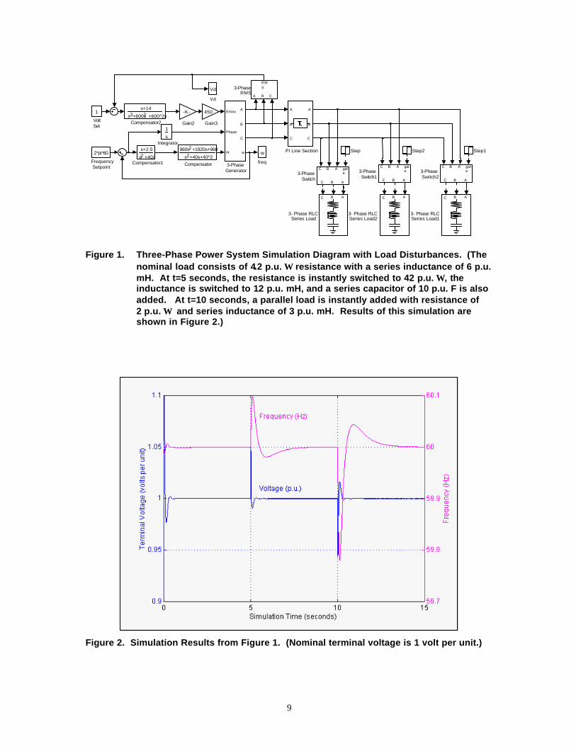
• RMS voltage control to ±6% of nominal with +1000% / -50% load disturbances (Figures 1and 2).

• Frequency control to ±0.35% of nominal with +1000% / -50% load disturbances (Figures 1and 2).

A synchronization control algorithm was also designed and tested for synchronizing and connect-ing multiple power plants onto a grid. (See Figures 3, 4 and 5.) To connect a power plant to thegrid, both the voltage and phase of the plant must match what is on the grid at the point ofconnection. Once these are matched, the power plant is connected. When the plant is firstconnected, it is not generating power; it is simply running at synchronous speed.

5 Isaac Horowitz and M. Sidi, "Synthesis of Feedback Systems with Large Plant Ignorance of Prescribed

Time Domain Tolerances," International Journal of Control , vol. 16, pp. 187-309, (1972).6 Isaac Horowitz, Quantitative Feedback Design Theory, vol. 1. QFT Publications, Boulder, CO, 1993,

Chapter 11.* Such as unstable and/or nonminimum phase plants (time delays), multiple-loop plants with a variety of

available internal sensing points how to divide up the feedback burden between them, multiple-inputmultiple-output plants (e.g., in a 3-by-3 plant, the nine closed-loop system response functions tocommands and disturbances can be individually controlled despite large uncertainties).

7 A. E. Bentley, "Quantitative Feedback Theory with Applications in Welding." International Journal ofRobust and Nonlinear Control, vol. 4, issue 1, January 1994.

8 A. E. Bentley, Control of Resistance Plug Welding Using Quantitative Feedback Theory. SAND94-0795A.Sandia National Laboratories, Albuquerque, NM.

9

w

freq

1

VoltSet

Vd

Vd

Step2 Step1Step

A

B

C

A

B

C

PI Line Section

s

1

Integrator

450

Gain3

-K-

Gain2

2*pi*60

FrequencySetpoint

s+14

s +600s +600^2s3 2

Compensator2

s+2.5

s +40s2Compensator1

960s +1920s+9602

s +40s+40^22

Compensator C B A gate

C B A

3-PhaseSwitch2

C B A gate

C B A

3-PhaseSwitch1

C B A gate

C B A

3-PhaseSwitch

Emax

Phase

Pr

A

B

C

w

3-PhaseGenerator

A B C

RMS3-Phase

RMS

C B A

3- Phase RLCSeries Load2

C B A

3- Phase RLCSeries Load1

C B A

3- Phase RLCSeries Load

Figure 1. Three-Phase Power System Simulation Diagram with Load Disturbances. (Thenominal load consists of 4.2 p.u. Ω resistance with a series inductance of 6 p.u.mH. At t=5 seconds, the resistance is instantly switched to 42 p.u. Ω , theinductance is switched to 12 p.u. mH, and a series capacitor of 10 p.u. F is alsoadded. At t=10 seconds, a parallel load is instantly added with resistance of2 p.u. Ω and series inductance of 3 p.u. mH. Results of this simulation areshown in Figure 2.)

Figure 2. Simulation Results from Figure 1. (Nominal terminal voltage is 1 volt per unit.)

10

Figure 3. Power System Simulation for Connecting a Slave Power Plant to a Power Grid.(The phase shift across the three-phase switch is forced to zero by adjustingthe phase of the slave power plant. The power plant voltage is also adjusted tomatch the line voltage at the switch. When both the phase and the voltage arematched, the three-phase switch is closed—connecting the slave power plantto the grid.)

pha

pha

Ramp

Vset

V1

V1

Gate

Phase Error

Fset

Vset

A

B

C

pha

SlavePower Plant

+

-

Error

Switch

PhaseDifference

A

B

C

A

B

C

PI Line Section

A

B

C

A

B

C

PI Line Section

Emax

Freq

A

B

C

MasterPower Plant

60

Freq. Set

gate

A

B

C

A

B

C

3-Phase Switch

A B C

RM

S

3-PhaseRMS

C B A

3- Phase RLCSeries Load1

C B A

3- Phase RLCSeries Load

A

B

C

A

B

C

PI Line Section

11

Figure 4. Simulation Results of Phase Control from Figure 3. (At t=1.25 seconds theslave power plant is connected to the grid.)

Figure 5. Voltage Control from Figure 3. (At t=1.25 s, the slave power plant is connectedto the grid.)

12

Power control (phase control) for a plant connected to a power system grid was also designed andsuccessfully tested. Once the power plant has been connected to the grid, the voltage control setpoint is increased to 1 volt per unit to keep the grid voltage within specification. The phase of thepower plant is also increased after it is connected so that the power plant begins to push poweronto the grid—rather than just running at synchronous speed without adding power (Figure 6).

The design of these controllers using QFT is briefly discussed below. The terminal voltage of thepower supply is given in Laplace format as

.2.18.0 and 175.0 where)( ≤≤≤≤+

= akas

ksV

The output of V(s) is also limited between 0.7 and 2.0. The root-mean-square of the voltage ismeasured and feedback to the voltage controller. This feedback sensor is characterized in theLaplace domain as

second.601

ere wh)(1 ==−

ττ

τ

se

sHs

The compensator for the voltage control system was designed using QFT as shown below:

5.0 and 600 ,14 ,450 : where)2(

)()(

22

2

1 ====++

+= ζω

ωζωω

akssa

asksG .

Figure 6. Simulation Results from Figure 3. Once the slave power plant has been con-nected to the grid (at t=1.25 seconds), the phase control set point is advancedsomewhat so that the power plant begins to push power onto the grid.

13

Because of load uncertainty in the power grid, the gain k is uncertain, as well as the timeconstant a. Thus, a family of plant equations that spans the range of uncertainty in the system isused to represent the voltage control system rather than using a single equation. The open-loopsystem L(s) = G1(s)·V(s) ·H1(s) is shown in Figure 7 in the format of a Bode plot of compensatedplant equations L(s). Note that the system has a phase margin of at least 65° and a gain margin ofat least 10 dB for all plants in the set.

Figure 7. Bode Plots of Open-Loop Voltage Control Plant V(s) with Compensator G1(s) andFeedback Sensor H(s). L(s) = G1(s)·V(s) ·H1(s).

The transfer function for the closed-loop or regulated voltage control system is given by

)()()(1)()(

)(11

1

sHsVsGsVsG

sT+

= .

The closed-loop voltage controller T(s) is plotted in Figure 8. Note the effect of feedback on thesystem uncertainty: for frequencies below the system bandwidth, the uncertainty has essentiallybeen eliminated. At higher frequencies, where system uncertainty is less important, theuncertainty is the same as for the open-loop system.

14

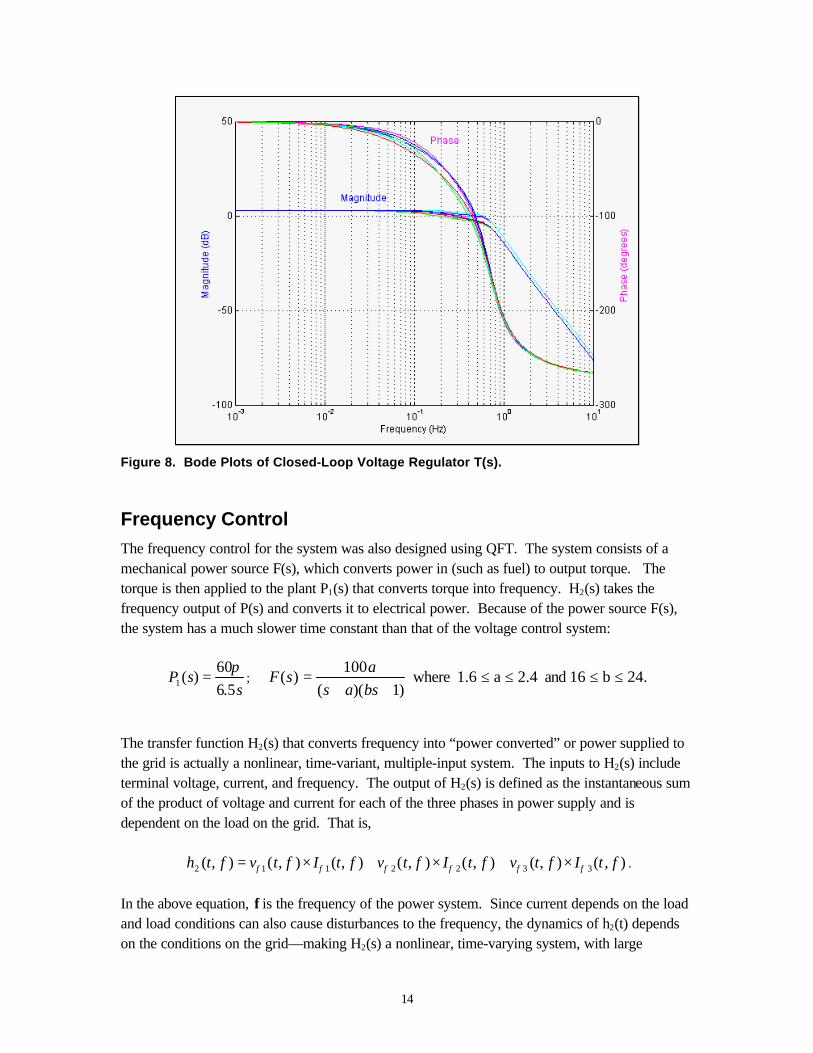
Figure 8. Bode Plots of Closed-Loop Voltage Regulator T(s).

Frequency ControlThe frequency control for the system was also designed using QFT. The system consists of amechanical power source F(s), which converts power in (such as fuel) to output torque. Thetorque is then applied to the plant P1(s) that converts torque into frequency. H2(s) takes thefrequency output of P(s) and converts it to electrical power. Because of the power source F(s),the system has a much slower time constant than that of the voltage control system:

ssP

5.660

)(1π

= ; 24.b16 and 2.4a1.6 where)1)((

100)( ≤≤≤≤

++=

bsasa

sF

The transfer function H2(s) that converts frequency into “power converted” or power supplied tothe grid is actually a nonlinear, time-variant, multiple-input system. The inputs to H2(s) includeterminal voltage, current, and frequency. The output of H2(s) is defined as the instantaneous sumof the product of voltage and current for each of the three phases in power supply and isdependent on the load on the grid. That is,

),(),( ),(),(),(),(),( 3322112 ftIftvftIftvftIftvfth φφφφφφ ×+×+×= .

In the above equation, f is the frequency of the power system. Since current depends on the loadand load conditions can also cause disturbances to the frequency, the dynamics of h2(t) dependson the conditions on the grid—making H2(s) a nonlinear, time-varying system, with large

15

uncertainties. However, these ill-behaved characteristics of our system can easily be accountedfor using QFT. As with uncertainty, nonlinearity and time variance can be rigorously quantifiedusing a set of linear, time-invariant equations or plants that fully characterizes the system H2(s)over its entire range of nonlinearity, time variance, and uncertainty. The set of equations isshown in the compensated frequency control Bode plots of Figure 9. Figure 9 shows the familyof equations that represents the open-loop transfer function of the frequency control system.(Two different compensators G2(s) and G3(s) were explored for frequency control. The G3(s)compensator was used in Figure 9.) Note that, all the plants in the system have at least 65° ofphase margin and a conditionally stable gain margin of at least +20/-15 dB. Figure 10 shows theclosed-loop feedback system. Also note the large decrease in uncertainty at low frequencybecause of feedback control (more than 30 dB in the open-loop system at f=0.001 Hz is cancelledout in the closed-loop system).

)4040)(40()12)(5.2(960

)(22

2

2 ++++++

=ssss

ssssG

)200200)(200()44)(2(000,480

)(22

22

3 ++++++

=ssss

ssssG

Figure 9. Bode Plots of Open-Loop Frequency Controller.

16

Figure 10. Bode Plot of Closed-Loop Frequency Control.

The phase controller uses almost the same compensator used for frequency control. The onlydifference is as follows. Phase is defined as the integral of frequency. In terms of Laplace, thephase-control plant P2(s) is equal to the frequency control plant P1(s) multiplied by 1/s; that is,P2(s) = P1(s)/s. Because of this extra integrator in the system plant, the integrator in the frequencycontrol compensator G3(s) is not used for phase control.

The phase controller is used in the slave power plant to match the frequency and phase of thepower grid. At the same time, the voltage controller servos the slave plant to match the voltage ofthe grid. Once both the voltage and phase are matched, the three-phase switch connects the slavepower plant to the power grid. At this point, the dynamics of the plant change considerably.When the plant is first connected, it is not actually generating any power; it is simply spinning atthe right frequency to match the grid. After being connected, the phase of the slave plant isadvanced to cause the plant to “push” power onto the grid. Because of the “inertia” of the grid,its loads, and other generators, the phase control plant becomes a highly underdamped systemwith a resonance at about 1.5 Hz. When considering the nonlinearities and uncertainties of thesystem, this becomes a very challenging system to control using conventional feedback controldesign techniques. However, using QFT greatly simplified the design for the phase controller.

The open-loop Bode plots for the phase controller are shown in Figure 11. Because of theunderdamped resonance at 1.5 Hz together with other plant uncertainty, it is difficult to read thegain and phase margin from the Bode plots in Figure 12. A preferable tool is thus employed in

17

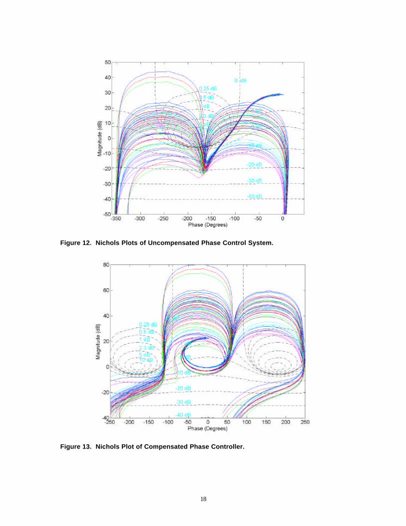
QFT design, namely, the Nichols plot. The Nichols plot contains the same information as does aBode plot but uses a more useful format (see Figures 12 and 13). Rather than plotting magnitudeand phase vs frequency, the Nichols plot shows phase vs magnitude as the frequency is variedfrom zero to infinity. When using the Nichols plot to design feedback systems, the Nyquistcriterion is satisfied by ensuring that the system crosses the 0 dB gain threshold “to the right” ofthe -180° phase threshold. Quantitative design margins can be assured by staying away from theclosed-loop magnitude contours that concentrically surround the 0 dB, -180° instability point.Note that the uncompensated phase control system shown in Figure 12 violates the Nyquistcriterion.

Figure 11. Bode Plot of Open-Loop Phase Controller.

18

Figure 12. Nichols Plots of Uncompensated Phase Control System.

Figure 13. Nichols Plot of Compensated Phase Controller.

19

Because of the added nonlinearity and uncertainty of the phase control system, the originalfrequency control compensator G2(s) design proved to be insufficient (with too little gain) foradequate phase control. The phase control compensator G4(s) improved on the frequencycontroller and led to the new frequency control compensator G3(s). Since the new frequencycontroller has much higher gain, it has significantly better performance than the originalcompensator. Thus, for phase control, we have G4(s) = sG3(s). The compensated phase controlsystem is shown in Figure 13. Note that all the plants in the system have at least 65° of phasemargin and a conditionally stable gain margin of at least +24/-5 dB. Also note in Figure 13 thatthe circular contours that surround the 0 dB, -180° instability point are repeated every 360° on theNichols chart. Thus, the compensator design needs must not only guarantee that the systemavoids the Nyquist instability point, but must also avoid the Nyquist point +360°. The Bode plotsof the closed-loop phase control system are shown in Figure 14.

Figure 14. Bode Plot of Closed-Loop Phase Controller.

20

Conclusions

Quantitative feedback theory provides a simple yet powerful philosophy for designing controlsystemsallowing the designer to optimize the system by making design tradeoffs withoutgetting lost in complex mathematics. The feedback systems were effective in reducing sensitivityto large and sudden changes in the power grid system. Voltage, frequency, and phase wereaccurately controlled, even with large disturbances to the power grid system.

Future research will apply QFT to distributive control of complex distributed generation scenarioson the power grid to minimize the effects of power transmission faults. The system will adjustpower grid parameters to ensure that none of the load limits on the existing power lines areexceeded when a power line is faulted (opened). A second important direction based on thiswork is to directly address the issue of minimizing or eliminating reliability margins. Theultimate objective is to reach system wide coordinated real-time control.

21

Distribution1 MS0188 LDRD Program Office, 1030 (Attn: Donna Chavez)1 MS0501 M. K. Lau, 23381 MS0501 A. E. Bentley, 23381 MS0741 M. L. Tatro, 62001 MS0710 A. A. Akhil, 62511 MS0710 J. D. Boyes, 62511 MS0451 S. G. Varnado, 65001 MS0785 R. L. Hutchinson, 65161 MS0785 J. E. Stamp, 65161 MS0455 R. S. Tamashiro, 651710 MS0455 R. E. Carlson, 65171 MS0455 J. J. Torres, 65171 MS9018 Central Technical Files, 8945-11 MS0612 Review & Approval Desk for DOE/OSTI, 96121 MS0899 Technical Library, 9616