SAMSI Astrostatistics Tutorial

More Markov chain Monte Carlo&

Demo of Mathematica software

Phil Gregory

University of British Columbia

2006

Bayesian Logical Data Analysis for the Physical Sciences outline

1. Role of probability theory in science2. Probability theory as extended logic3. The how-to of Bayesian inference4. Assigning probabilities5. Frequentist statistical inference6. What is a statistic?7. Frequentist hypothesis testing8. Maximum entropy probabilities9. Bayesian inference (Gaussian errors)10. Linear model fitting (Gaussian errors)11. Nonlinear model fitting12. Markov chain Monte Carlo13. Bayesian spectral analysis14. Bayesian inference (Poisson sampling)Appendix A. Singular value decompositionAppendix B. Discrete Fourier TransformAppendix C. Difference in two samplesAppendix D. Poisson ON/OFF detailsAppendix E. Multivariate Gaussian from maximum entropy.

Contents:

Outline

1. Introduce MCMC and parallel tempering2. Technical difficulties 3. Return to simple spectral line problem4. Tests for convergence

5. Exoplanet examples

6. Model comparison (global likelihoods)

1

2

3

4

5

6

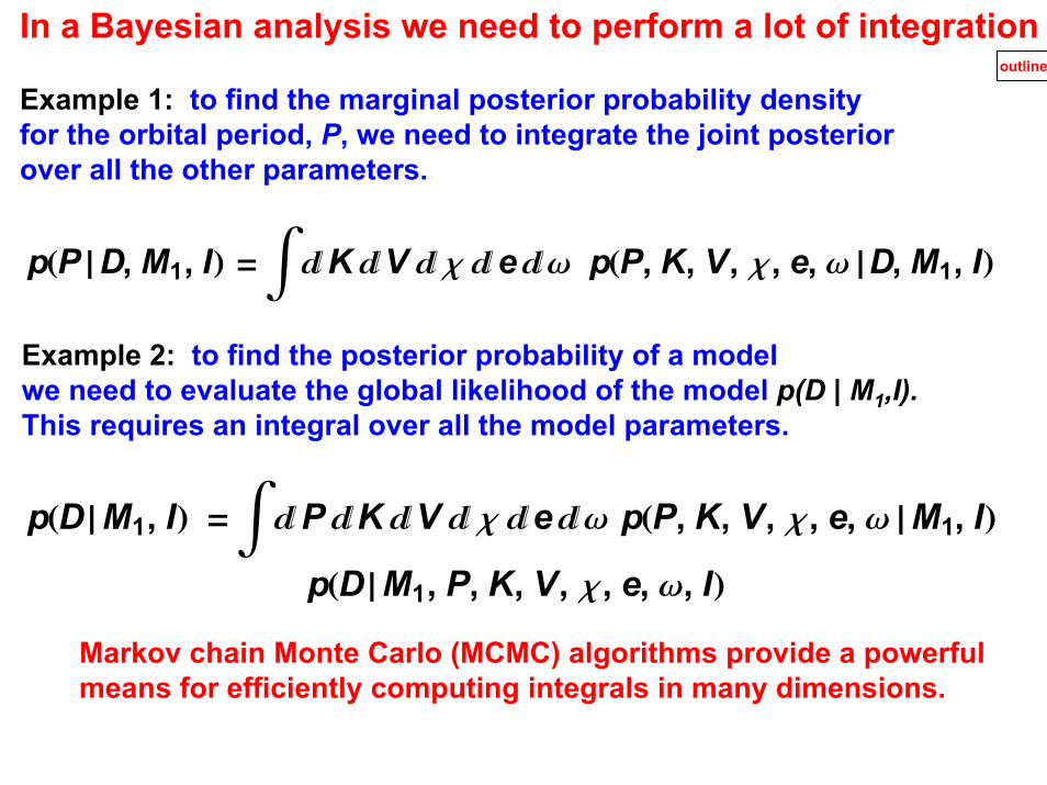
In a Bayesian analysis we need to perform a lot of integration

Example 1: to find the marginal posterior probability densityfor the orbital period, P, we need to integrate the joint posteriorover all the other parameters.

outline

p P D, M1, I = ‚ K ‚ V ‚ c ‚ e ‚ w p P, K, V, c, e, w D, M1, I

Example 2: to find the posterior probability of a modelwe need to evaluate the global likelihood of the model p(D | M1,I).This requires an integral over all the model parameters.

p D M1, I = ‚ P ‚ K ‚ V ‚ c ‚ e ‚ w p P, K, V, c, e, w M1, I

p D M1, P, K, V, c, e, w, I

Markov chain Monte Carlo (MCMC) algorithms provide a powerfulmeans for efficiently computing integrals in many dimensions.

outline

MCMC to the rescueIn straight Monte Carlo integration independent samples are randomly drawn from the volume of the parameter space. The price that is paid for independent samples is that too much time is wasted sampling regions where posterior probability density is very small. Suppose in a one-parameter problem the fraction of the time spent sampling regions of high probability is 10-1. Then in an M-parameter problem, this fraction could easily fall to 10-M.

MCMC algorithms avoid the requirement for completely independentsamples, by constructing a kind of random walk in the model parameter space such that the number of samples in a particular region of this space is proportional to the posterior density for that region.

The random walk is accomplished using a Markov chain, whereby the new sample, X{t+1} , depends on previous sample Xt according to an entity called the transition probability or transition kernel, p(X{t+1} |Xt). The transition kernel is assumed to be time independent. The remarkable property of p(X{t+1} |Xt) is that after an initial burn-in period (which is discarded) it generates samples of X with a probability density equal to the desired posterior p(X|D,I).

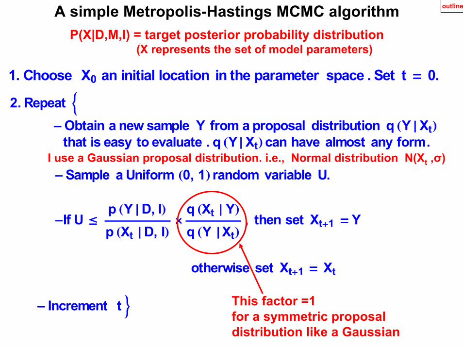
A simple Metropolis-Hastings MCMC algorithmP(X|D,M,I) = target posterior probability distribution

(X represents the set of model parameters)

outline

1. Choose X0 an initial location in the parameter space . Set t = 0.

2. Repeat :- Obtain a new sample Y from a proposal distribution q HY » XtL

that is easy to evaluate . q HY » XtLcan have almost any form.

- Sample a Uniform H0, 1L random variable U.

-If U £p HY » D, ILp HXt » D, IL

âq HXt » YLq HY »XtL

, then set Xt+1 = Y

otherwise set Xt+1 = Xt

- Increment t > This factor =1for a symmetric proposal distribution like a Gaussian

I use a Gaussian proposal distribution. i.e., Normal distribution N(Xt ,σ)

outline

Conditions for convergence

Remarkably, for a wide range of proposal distributions q(Y |X), the Metropolis-Hastings algorithm generates samples of X with a probability density which converges on the desired target posterior p(X|D, I), called the stationary distribution of the Markov chain.

For the distribution of to converge to a stationary distribution, the Markov chain must have three properties (Roberts, 1996).

1. It must be irreducible. That is, from all startingpoints, the Markov chain must be able (eventually) to jump to all states in the target distribution with positive probability.

2. It must be aperiodic. This stops the chain from oscillatingbetween different states in a regular periodic movement.

p JX”÷ »D, IM p JX

”÷ … X”÷'M = p JX

”÷' … D, IM p JX

”÷' …X”÷

3. It must be reversible.

M

�4 �2 0 2 4 6 8 10

X1

�4

�2

0

2

4

X2

Σ�10

�c�

�4 �2 0 2 4 6 8 10

X1

�4

�2

0

2

4

X2

Σ�0.1

�a�

�4 �2 0 2 4 6 8 10

X1

�4

�2

0

2

4

X2

Σ�1

�b�

In this example theposterior probability distribution consists of two 2 dimensional Gaussians

A comparison of the samples from three Markov Chain Monte Carlo runs using Gaussian proposal distributions with differing values of the standard deviation.

outline

50 100 150 200 250 300Lag

0

0.2

0.4

0.6

0.8

1X

2A

CF

10

Σ � 1

Σ � 0.1

A comparison of the autocorrelation functions for three Markov Chain Monte Carlo runs using Gaussian proposal distributions with differing values of the standard deviation.

outline

outline

The simple Metropolis-Hastings MCMC algorithm can run into difficulties if the probability distribution is multi-modal with widelyseparated peaks. It can fail to fully explore all peaks which contain significant probability, especially if some of the peaks are very narrow.

One solution is to run multiple Metropolis-Hastings simulations in parallel, employing probability distributions of the kind

β = 1 corresponds to our desired target distribution. The others correspond to progressively flatter probability distributions.

p HX »D, M, b, IL = p HX » M, IL p HD »X, M, ILb H0 < β b 1L

I learned about parallel tempering from this book.

outline

At intervals, a pair of adjacent simulations are chosen at random and a proposal made to swap their parameter states. The update can be accepted/rejected with a Metropolis-Hastings criterion. At time t, simulation is in state and simulation is in state . If the swap is accepted by the test given below then these states are interchanged. Accept the swap with probability

The swap allows for an exchange of information across the ladder of simulations.

In the low β simulations, radically different configurations can arise, whereas at higher β, a configuration is given the chance to refine itself.

Final results are based on samples from the β = 1 simulation.Samples from the other simulations can be used to evaluate the Bayes Factor in model selection problems.

outline

Technical Difficulties

1. Deciding on the burn-in period.

2. Choosing a good choice for the characteristic widthof each proposal distribution, one for each model parameter.

For Gaussian proposal distributions this means pickinga set of proposal σ’s. This can be very time consuming for a large number of different parameters.

3. Deciding how many iterations are sufficient.

4. Deciding on a good choice of tempering levels (β values).

MCMCNonlinearModelFittingProgram

Data Model Prior informationD M I

Target PosteriorpH8Xa<»D,M,IL

Control systemparameters

__________________________n1 = major cycle iterationsn2 = minor cycle iterationsl = acceptance ratiog = dampingconstant

n = no. of iterations8Xa<init = start parameters8sa<init = start proposal s's8b< = Temperinglevels

- Control systemdiagnostics- 8Xa< iterations- Summarystatistics- Best fit model & residuals- 8Xa< marginals- 8Xa< 68.3% credible regions- pHD»M,IL global likelihood

for model comparison

Schematic of a Bayesian Markov Chain Monte Carlo program for nonlinear model fitting. The program incorporates a control system that automates the selection of Gaussian proposal distributon σ’s.

outline

Return to simple spectral line problem outline

Now assume 4 unknowns line center frequency, T, line width, and an extra noise term with unknown standard deviation

Parameters f, T, lw, s

All channels have Gaussian noise characterized by σ = 1 mK. The noise in separate channels is independent. The line center frequency ν0 = 37.

outline

Tests for convergence

1. Examine plots of the MCMC iterations for each parameter.

2. Divide the post burn-in iterations into two halves and plot one on top of the other using different colors.

3. Compute the Gelman-rubin statistic for each parameter from the repeated runs.

0 20000 40000 60000 80000Iteration

4.2

4.4

4.6

4.8

5

w

0 20000 40000 60000 80000Iteration

05

1015202530

s

0 20000 40000 60000 80000Iteration

0

0.02

0.04

0.06

0.08

c

0 20000 40000 60000 80000Iteration

0.4

0.5

0.6

0.7

0.8

e

0 20000 40000 60000 80000Iteration

110

120

130

140

150

KHm

s-1 L

0 20000 40000 60000 80000Iteration

-45-40-35-30-25-20-15-10

VHm

s-1L

0 20000 40000 60000 80000Iteration

-47-46-45-44-43-42-41-40

goL01H

roirPµ

ekiLL

0 20000 40000 60000 80000Iteration

127

127.5

128

128.5

129

PHd

LTests for convergence

Compare iterationsfrom

multiple chains

For each parametercompute

Gelman-Rubin statistic

GR should be close to 1.0

Measured GR values < 1.02

outline

Mean within chain variance W =1

m Hh - 1L ‚j=1

m

‚i=1

h

Iq ji - q j

êêM2

Between chain variance B =h

m- 1 ‚j=1

mHq jêê

- qêêL2

Estimated variance V`

HqL =ikjj1 -

1h

y{zz W +

1h

B

Gelman- Rubin statistic = $%%%%%%%%%%%%V`

HqLW

Let q represent one of the model parameters.

Let q ji represent the ith iteration of the jth chain.

Extract the last h post burn-in iterations for each simulation.

The Gelman - Rubin statistic should be close to 1.0 He.g. < 1.05Lfor all paramaters for convergenceRef : Gelman, A.and D.B.Rubin H1992L' Inference from iterative

simulations using multiple sequences Hwith discussionL',Statistical Science 7, pp. 457 − 511.

outlineGelman-Rubin Statistic

0 100000 200000 300000 400000 500000 600000Iteration

00.10.20.30.40.50.6

e

0 100000 200000 300000 400000 500000 600000Iteration

0123456

w

0 100000 200000 300000 400000 500000 600000Iteration

-120-100

-80

-60-40-20

0

VHm

s-1 L

0 100000 200000 300000 400000 500000 600000Iteration

-0.3-0.2-0.1

00.10.20.30.4

c

0 100000 200000 300000 400000 500000 600000Iteration

50100150200250300350400

PHd

L0 100000 200000 300000 400000 500000 600000

Iteration

6080

100120140160180

KHm

s-1L

0 100000 200000 300000 400000 500000 600000Iteration chain Hb = 1.L

-180-160-140-120-100

-80-60-40

goL01

HroirP

µekiLL

0 100000 200000 300000 400000 500000 600000Iteration

-52.5-50

-47.5-45

-42.5-40

-37.5

goL01

HroirP

µekiLL

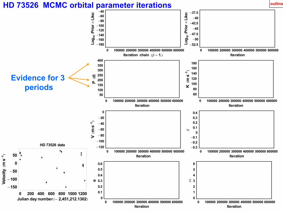
HD 73526 MCMC orbital parameter iterations

Evidence for 3 periods

0 200 400 600 800 1000 1200Julian day number H- 2,451,212.1302L

-150

-100

-50

0

50

yticoleVHm

s-1L

HD 73526 data

outline

outline

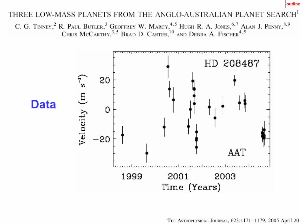
Data

Evidence for a second planet in HD 208487 outline

Gregory, P. C. (2005), AIP Conference Proceeding 803, p. 139, 2005

0 500 1000 1500 2000Julian day number H- 2,451,034.1784L

-30

-20

-10

0

10

20

30

40

yticoleVHm

s-1L

Best fit P1 = 129.517 ; K1 = 15.9778 ; V = 7.92451 ; c1 = 0.184585 ; e1 = 0.224581 ; w1 = 2.20511 ;P2 = 998.085 ; K2 = 9.81886 ; c2 = 0.723248 ; e2 = 0.189448 ; w2 = 2.74554

c2u = 0.83RMS residual = 4.2 m s-1

priors

P1 = 129.52 d e1 = 0.22

P2 = 998 d= 2.73 yr

e2 = 0.19

0 0.5 1 1.5 2P2 Orbital phase

−10

0

10

20

yticoleVHm

s-1L

HbL

0 0.5 1 1.5 2P1 Orbital phase

−30

−20

−10

0

10

20

30

yticoleVHm

s-1L

HaL

HD 208487outline

Model compare

outline

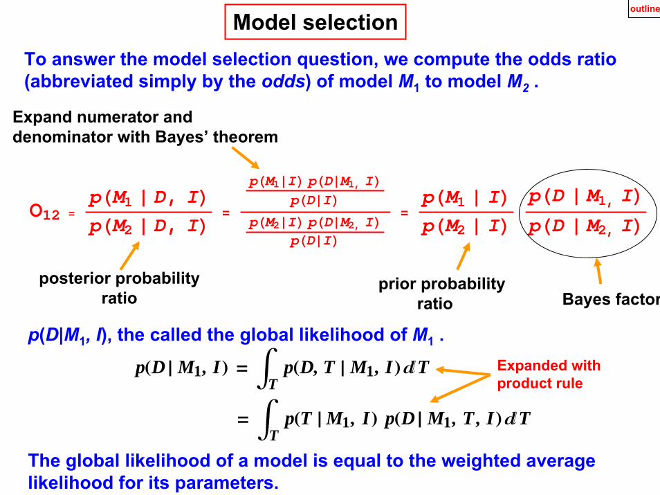
To answer the model selection question, we compute the odds ratio (abbreviated simply by the odds) of model M1 to model M2 .

Model selection

Expand numerator and denominator with Bayes’ theorem

prior probabilityratio Bayes factor

posterior probabilityratio

O12 =pHM1 » D, ILpHM2 » D, IL =

pHM1»IL pHD»M1, ILpHD»IL

pHM2»IL pHD»M2, ILpHD»IL

=pHM1 » ILpHM2 » IL

pHD » M1, ILpHD » M2, IL

pHD » M1, IL = ‡T

pHD, T » M1, IL‚T

= ‡T

pHT » M1, IL pHD » M1, T , IL‚T

p(D|M1, I), the called the global likelihood of M1 .

The global likelihood of a model is equal to the weighted averagelikelihood for its parameters.

Expanded with product rule

outline

Model selection

Herewecompute the log of theglobal likelihood of themodel, log@p HD » M1, ILD .log@p HD » M1, ILD = ‡ Xln pHD » ME, P, K, V, c, e, w, IL\b ‚ b

Xln pHD » ME , P, K, V, c, e, w, IL\b

= expectation value of ln @pHD » ME, P, K, V, c, e, w, ILD for given b

=1n

‚t=1

nln@p HD » M1, Pt,b , Kt,b , Vt,b , ct,b , et,b , wt,b , ILD

where n = number of MCMC iterations.

See my book forderivation

One way to compute the global likelihood of the mode,

Here we compute the log of the global likelihood of the model, log@p HD » M1, ILD .log@p HD » M1, ILD = ‡ Xln pHD » ME, P, K, V, c, e, w, IL\b ‚ b

Xln pHD » ME , P, K, V, c, e, w, IL\b

= expectation value of ln @pHD » ME, P, K, V, c, e, w, ILD for given b

=1n

‚t=1

nln@p HD » M1, Pt,b , Kt,b , Vt,b , ct,b , et,b , wt,b , ILD

where n = number of MCMC iterations.

1. µ 10-13 1. µ 10-10 1. µ 10-7 0.0001 0.1Log b

-40000

-30000

-20000

-10000

0

XnlpH

D»M

E,P,

K,V,

c,e,

w,IL

\ 30 tempering levels

See my book forderivation

One way to compute the global likelihood of the mode,

outline

1. µ 10-13 1. µ 10-10 1. µ 10-7 0.0001 0.1Log b

-40000

-30000

-20000

-10000

0Xnl

pHD»

ME,

P,K,

V,c,

e,w

,IL\

0.01 0.02 0.05 0.1 0.2 0.5 1Log b

-400

-300

-200

-100

0

XnlpH

D»M

E,P,

K,V,

c,e,

w,IL

\

Blow-upoutline

p(M1J|D,I) = 1.4 x 10-55 (from tempering levels)p(M1J|D,I) = 2.5 x 10-55 (from restricted Monte Carlo integration)p(M0s|D,I) = 1.5 x 10-59 (from numerical integration)