Sampling for Particle Size Analysis

www.malvern.co.uk

This product support brochure applies to thefollowing Malvern Instruments’ products:

Mastersizer 2000

Mastersizer S

Mastersizer Micro

Mastersizer Microplus

Author: Dr Alan RawleMalvern Instruments, UK

Like most things in life you get out what you put in.This cannot apply morestrongly than in the situation of particle sizing where “garbage in = garbage out”is an appropriate maxim.

If we consider a pack of cereal such as museli, it is quite obvious that the last two teaspoons taken from the packet are not the same as the first two. Forsystems like this, then it is clear even to the non-scientist that segregation hasoccurred (“the contents of the package may have settled during transit”) and thatthe properties of the first and last samples from the packet are totally different.As scientists (hopefully!) we need to quantify these effects and decide when thisphenomenon is important from a statistical point of view and when it is not.A more serious example of the “garbage in = garbage out” situation was thatresulting from the confusion in UK Government laboratories between cow andsheep brains (“bovine or ovine?”) resulting in the causes and transmittal mode of BSE being misinterpreted.This prompted the quotation within the editorial of the December 2001 issue of Chemistry in Britain that “Sample integrity andsound data analysis are essential cornerstones of valid analyses for decision making”.

Thus before we even begin the statistical evaluation, we need to ask ourselves thereason or objective behind the analyses12 (because one analysis on its own wouldbe statistically perfect):

What do we want to know?

Why do we need this information?

What happens to the results?

What actions may follow (and the economic and other implications) of theresults being circulated?

We also need to ask ourselves whether we require a bulk powder measurementdesigned to investigate say, for example, flowability, filter blockage or dustingtendency or whether we are concerned with a primary size of the particle systemas the latter may control dissolution rate, gas absorptionand chemical reactivity.We need to be aware that theenergies generated in any particle size “dispersion unit”or accessory are likely to be many times larger than those within a production environment. For example,a hydrocyclone operates only at a few ms-1 in contrast to the typical 70W of a low powered sonication bath.

A good illustration of the effect of segregation can be seen in any large mine spoil heap or, more conveniently,in small demonstrators available from Jenike and Johanson:

2

Sampling for Particle Size Analysis—

Introduction

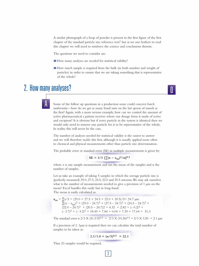
A similar photograph of a heap of powder is present in the first figure of the firstchapter of the standard particle size reference text1 but as no one bothers to readthis chapter we will need to reinforce the science and conclusions therein.

The questions we need to consider are:

How many analyses are needed for statistical validity?

How much sample is required from the bulk (in both number and weight ofparticles) in order to ensure that we are taking something that is representativeof the whole?

3

2. How many analyses? Q

A Some of the follow up questions in a production sense could concern batchuniformity—how do we get as many brasil nuts on the last spoon of museli as the first? Again, with a more serious example, how can we control the amount ofactive pharmaceutical a patient receives where our dosage form is made of activeand excipient? It is obvious but if every particle in the system is identical then wewould only need to remove one particle for it to be representative of the whole.In reality this will never be the case.

The number of analyses needed for statistical validity is the easiest to answer and we will therefore tackle this first, although it is usually applied more often to chemical and physical measurements other than particle size determination.

The probable error or standard error (SE) in multiple measurements is given by:

SE = 2/3 [∑(x – xm)2/n]0.5

where x is any sample measurement and xm the mean of the samples and n thenumber of samples.

Let us take an example of taking 5 samples in which the average particle size is(perfectly measured) 29.0, 27.5, 24.5, 22.0 and 20.5 microns.We may ask ourselveswhat is the number of measurements needed to give a precision of 1 µm on themean? Excel handles this easily but in long-hand:The mean is easily calculated as:

xm = ∑x/5 = (29.0 + 27.5 + 24.5 + 22.0 + 20.5)/5= 24.7 µm∑(x – xm)2 = (29.0 – 24.7)2 + (27.5 – 24.7)2 + (24.5 – 24.7)2 + (22.0 – 24.7)2 + (20.5 – 24.7)2 = 4.32 + 2.82 + (- 0.2)2 + (- 2.7)2 + (- 4.2)2 = 18.49 + 7.84 + 0.04 + 7.29 + 17.64 = 51.3

The standard error is 2/3 X (51.3/5)0.5 = 2/3 X (10.26)0.5 = 2/3 X 3.20 = 2.1 µm

If a precision of ± 1µm is required then we can calculate the total number ofsamples to be taken as:

2.1/1.0 = (n/5)0.5 = 22.1

Thus 23 samples would be required.

This is not the usual situation that we are trying to deal with in particle sizeanalysis. Indeed in the above situation we are so subject to the vagaries of thesampling method (are these independent samples?) and the dispersion method,that this answer is almost meaningless. Besides the British Standard Customer(BSC) will only take one measurement anyway…

The more important question that is usually requiring a statistical answer is theminimum amount of sample that would be needed to ensure that it could berepresentative of the whole or at least a rough guide to what we would expect to need. Clearly there will be a number of assumptions needed to answer thisparticular issue. It is an issue that has occupied chemical engineers since 1880 or so (e.g. Reed).Taggart’s Handbook of Mineral Dressing (1948) gives anonogram for minimum weight (based on type of ore—rich or lean—andparticle size) based on the assumptions of Richard (1903) which has been the reference in the mining industry from thereon. Gy’s work2, 3 (1953, 1982) is extensively quoted where the weight of sample required is proportional to da where the exponent is a variable between 2 and 3 but theoretically 3 (the number – volume/mass relationship).The constant of proportionality isdependent on the accuracy desired, the homogeneity and value of the ore.

Even later pragmatic work by Kraft (1978 and summarised in 4) is of little value as multiple determinations (he recommends 20 and talks of 1 kg shovels full!) are needed and this is not helpful to engineers seeking ballpark figures beforebeginning an analysis.

So we need to seek more practical solutions. Let us start from the basis that werequire a standard error of 1% and that the mid-point of the highest size band is known (d99.5 is close enough unless the pedants insist on a more accurategeometrical midpoint assuming a logarithmic spacing of size classes).We will furtherassume that this highest size band contains 1% of the material by mass or volume(constant density assumed of a single component system).This is probably reasonableif the customer believes that 100 size classes equate to resolution! So we cancalculate the number of particles required in this highest size band:

1/100 = 1/n0.5

leading to a need for 10000 particles in the highest size band.The number 10000is interesting (although it does not provoke a large entry in the Book of InterestingNumbers5. In fact it provokes no entry at all in the aforementioned volume) as it isthe same number of images (not particles) that NBS (National Bureau of Standards)stated that was needed for statistical validity in image analysis6:

“S(tandard error) is proportional to N-1/2 where N is the total number of particlesmeasured…This consideration implies that image analysis may require the analysisof on the order of 10000 images to obtain a satisfactory limit of uncertainty”(p718, paragraph 1).

4

Weight of sample versus maximum size

0

20

40

60

80

100

120

140

160

180

0 100 200 300 400 500 600

Mid point of last size band

Wei

ght

of sa

mple

(g)

Weight of sample and maximum size

0

0.2

0.4

0.6

0.8

1

1.2

1.4

0 20 40 60 80 100 120

Mid point of last size bandMin

imun w

eigh

t of sa

mple

req

uir

ed (

g)

This minimum number of particles for 1% or better SE is then more useful aswith knowledge or assumptions about the particle density, a spreadsheet is easilyconstructed and we are able to get a feel for the sort of sample size required:

3. How much weight/mass of sample is required? Q

A

More rigorous theoretical solutions are provided by Masuda and Gotoh7 andenhanced by Wedd8, but the figures crudely calculated above in the spreadsheetare in the same ballpark.We note that the old maxim that 75 or 100 µm providedthe point at which sampling became the predominant error in particle sizeanalysis is easily understood if a sample size of around 1g is assumed for manyanalytical techniques. See below:

5

D Diameter Radius Density Weight in top Total weight (g)

(µm) (cm) (cm) (g/cm3) size fraction (g) (= Last column X100)

1 0.0001 0.00005 2.5 1.31358E-08 1.31358E-06

10 0.001 0.0005 2.5 1.31358E-05 0.001313579

100 0.01 0.005 2.5 0.013135792 1.313579167

1000 0.1 0.05 2.5 13.13579167 1313.579167

10000 1 0.5 2.5 13135.79167 1313579.167

200* 0.02 0.01 3.15 0.13240878 13.24

80 0.008 0.004 3.15 0.008474162 0.85

This is the weight This is where 1% of 10000 particles of the particles are

in the top size band

Assuming spheres

*This represents a typical cement

4. Reliability of sampling methods

We can then decide on appropriate sampling regimes for the mass of materialthat we take as a (minimum) base sample calculated from the above spreadsheet.Note that it would be meaningless if we have material up to say 500 µm in thesample to try to measure 50 mg or so (1 particle?).At 1mm we need over 1 kg ofmaterial to have 10000 particles in the highest size band.To examine Allen’s(frequently quoted) summary of sampling methods at this stage is extremelyeducational (and will lead on to answering the question “How do we take thesample as opposed to how should we take the sample?”):

Reliability of selected sampling methods using a 60:40 sand mixture

Sampling technique Standard deviation

Cone and quartering 6.81

Scoop sampling 5.14

Table sampling 2.09

Chute slitting 1.01

Spinning riffling 0.146

Random variation 0.075

Taken from Table 1.5 page 38,T.Allen Particle Size Measurement, 5th Edition Volume 1

Chapman and Hall 1997 ISBN 0 412 72950 4

The most common way that sample are taken within industry (scoop or spatula)is subject to an expected standard deviation of just over 5%.Thus if we are usingthis technique we could not expect to specify our material to better than 20% orso (3σ covering 99.7% of a Gaussian distribution is around 16% with this method).The choice is either to employ a spinning riffler for sample division or widen the permitted specification.Thus the recommendations in ISO133209 Section 6.4 which deal with repeatability allow for 3 consecutive aliquots a deviation of 3% for the D50 and 5% for the D10 and D90 in the tails of the distribution.This could only be achieved for samples that have either been correctly dividedor were small enough that sufficient particles were in the highest size band.Thusthis is a reasonable check on the homogeneity or otherwise of our sample ratherthan on the performance of the instrument. By the way, the doubling of the“permitted” deviations under 10 µm is more related to control of the dispersionof the material than to sampling.

6

7

5. Practical sampling methods

Back to our important question on the best way to take a sample. Spinning rifflershave been around for at least 100 years. Here is an early version made of woodand buckets10:

The modern version is with stainless steel trays or glass bottles:

From companies such as Retsch or Microscal units can be obtained that will deal with 10 g – 100 kg of sample. These are conveniently and usually used in thelaboratory in order to split a primary sample into a size suitable for measurementfor, say, XRF or laser diffraction. One must realise at this stage that this method isthe only one capable of producing less than 1% sample to sample variation. If onedoes not employ a rotary dividing technique and one wants less than 1% coefficientof variation sample-to-sample then this will certainly end in tears.The otheralternative is to use scoop sampling and work with a larger acceptable specification.

Vibrating Sample Hopper

Sample Trays

Cone and quartering, although reasonably common, should never be employed11:

Chute riffling is barely acceptable (just over 1% RSD):

Riffle sample divider(Reproduced by permission from BS 5309, Part 4, 1976)

So what if we have a large mine dump or a glacial moraine (“so what?” you may say):

8

123456

60˚

Alternative sections collectedon each side

7891011

119

75

31

12

What are the rules for sampling here? Allen provides two words of advice—don’tand never. However, this is more flippant than practical (thus appeals to me!) andwe need to outline the golden rules of sampling as expounded by Allen andothers on many occasions:

Take the sample when the product is moving.This could be when a large drum or container is packed. Once in the drum we’re then subject to any settling that takes place during transport. If this is not practical then we’re back to the choice of either spinning riffler or a wider specification or experimentalevidence/statistics on the basis or real-world experiments

Take the entire stream for a short period rather than part of the stream for along period.This is to avoid taking samples say at the edge where air currentscould influence what is sampled or in the middle of a pipe where particle sizedistribution is not the same as close to the edges.This indicates that cross-stream and Vezin type samplers must be statistically better than putting a fixedprobe into a stream.

The above photographs show the boulder-like particles (larger than a man togetherwith the sub-micron rock flour in suspension at the Franz Josef Glacier in NewZealand). In all cases repeated samples (to reiterate, Kraft’s recommendation is 20)should be taken to assess the homogeneity or otherwise and to get a feeling for theexpected variations. Even this may have problems with friable or fragile material(e.g. needle-like pharmaceutical) where the simple act of sampling a barrel orcontainer of powder with a spear is likely to cause damage to the particles:

Open-sided sampling spear and divided spear for dry, free-running powders (Reproduced by permission from ‘The Sampling of Bulk Materials’, by R. Smith and G.V. James,The Royal Society of Chemistry, London, 1981)

9

TYPICAL CROSS SECTIONS

For mines and piles of materials then trenches can be dug and the literature (e.g. 1 and 11) contains details of these methodologies. However, actual measurementswill indicate the huge spread of particle sizes in such situations and would be morepractical than the flippant “Don’t/never!” advice.

Slurry sampling is potentially much worse than sampling of dry powders in that segregation or settling is almost certain to be occurring. Extreme care andevaluation needs to be taken when sampling from a pipe or in a wet grindingsituation as it is a virtual impossibility that the system is homogenous from a particle size point-of-view A Burt sampler is normally recommended for slurry or suspension sampling:

The Microscal suspension sampler, 100 mL to 10 mL

10

6. Experimental results

It is reasonable now to examine some practical results of sampling that we havecarefully undertaken at Malvern Instruments on purified teraphthalic acid (PTA)both as a dry powder and as a prepared slurry in water.The material is quite largeand exhibits the potential for significant sampling errors.The recommendations ofISO13320 were followed in that, for riffled samples, the complete sampled sub-lotwas used for the measurement. Repeatability was assessed for wet measurements(the marks on the plots indicating the full set of results) by taking 10 consecutiverepeat measurements.

Consecutive dry sampling of large material (PTA)

20

70

120

170

220

270

1 2 4 6 8 103 5 7 9 11

Record number

Trend graph

d (0.1)

d (0.5)

d (0.9)

Mean

SD

% Variation

37.88

3.03

7.99

121.21

4.05

3.34

257.17

13.68

5.32

D10 D50 D90

Par

amen

ter

For successive scoop sampled aliquots we see standard deviations in line with thosenoted by Allen:

11

We note too that the effect is only just seen at the D90 end of the distribution—there is virtually no effect on the smaller D10 and median, D50, points.There is a gradual fall in D90 as we remove the larger material (the nuts and raisins in themuseli), which sits on top of the pile, but one can see why this type of (subtle)trend is rarely noted. In the case of a slurry sample we get an interesting step-effect:

The initial samples were taken by pipette withdrawal from a well and continuouslystirred (magnetic stirrer) slurry of the material contained in a beaker.This materialin suspension shows little change.The step is at the point when no liquid remainedand one started to sample, by spatula, the paste sitting at the bottom of the beaker.This shows segregation effects by the gradual rise in key parameters shown above.

D10

D50

D90

Consecutive wet sampling of large material (PTA) Sedimentation in Sample

0

100

200

300

400

0 20 4010 30 50Sample number

Siz

e (M

icro

ns)

Mean

Standard deviation

% RSD

Number of samplings

52.11

8.83

16.34

40

141.12

22.22

15.75

316.02

49.80

15.76

D10 D50 D90

In terms of samples extracted by spinning riffler and measured in their entirety wesee no discernible trends in D90 over the 25 trays of the riffler:

12

We note that in practical terms I cannot approach the wonderful (ideal?!) s.d.figures quoted by Allen but I can considerably improve on the values generated bysimple scoop or slurry sampling and remove any systematic variation.

7. Implications for product homogeneity and mixing

Last, but by no means least in practical terms let us examine some rules of thumb forproduct homogeneity.The author has witnessed a large pharmaceutical manufacturerbeing unable to control the dose of active ingredient with an inactive base materialand this type of observation has been reported in the literature on numerousoccasions13, 14.This was simply due to the large differences in sizes—micronizeddrug together with inactive up to 1000 µm or so.The general rule here is that wewill reduce the propensity to “unmix” by mixing particle size distributions that donot differ by more than 0.3 – 1.4 (or 40% or so).The solution for the pharmaceuticalcustomer above was obvious—micronize both the active and inactive.As an exampleif the drug is of mean size 50µm then to introduce a filler of 100 µm is inadvisable.Rather the filler should be within the range 15 – 70 µm. Small particles or a broaddistribution aid packing and compaction strength and can help flowability issues.When small particles adhere to coarse ones then more homogenous mixtures canresult but this could be in conflict of making smaller drugs for more rapid dissolution.As is usually the case a balance must be sought between particle size distribution,flowability and homogeneity.

A corollary to this relates to the recommendations within ISO13320 relating toverification of laser diffraction equipment. Here spherical materials of no morethan 1 decade in diameter distribution are stated to be preferred.Although a 1 – 10 µm(or 10 – 100 µm) range in diameter does not appear significant it is equivalent to a1000-fold difference in weight or volume so segregation is a real possibility unlessthe particles are particularly small where attractive forces bind them together.

USE OF SPINNING RIFFLER

0

100

200

300

400

0 2010 30

Riffled sampling variation

Record number

Siz

e (M

icro

ns)

Mean

Standard deviation

% RSD

Number of samplings

52.78

1.97

3.74

25

138.18

4.36

3.15

325.16

6.13

1.88

D10 D50 D90

D10

D50

D90

13

8. Implications for particle size measurement by laser diffraction

Measurement by laser diffraction is characterised by a number of requirementsthat need to be met.

To avoid multiple scattering (a number/concentration/size constraint) thenmeasurements are normally run at fairly low concentrations—typically 0.01 – 0.001volume %.A pharmaceutical manufacturer may ask “What is the smallest amount of material that can be measured?” and may be wanting to minimise the amount of sample (expensive R & D material?) or exotic or dangerous or expensive solvent (at least for disposal). Hence the unwary customer and salesperson may be ridingalong the possibly dangerous track of specifying a small volume dispersion unitwithout remembering the requirements for adequate sample mass and also the needto keep material adequately in suspension. Failure to control either leads to lack ofrepeatability (consecutive measurements—the small number of large particles is notintegrated a sufficient number of times or the larger particles are only occasionally“kicked” through the laser beam) and poor reproducibility (sub-sample to sub-sample variation based on the homogeneity or otherwise of the sample).

With a small volume unit we may only be using a small volume of dispersant andthus we could never load the amounts of material required for adequate sampling(at reasonable levels to ensure multiple scattering does not occur15) into the unitespecially if the sample has any polydispersity.And if we sub-sample from ourstarting material there is an enormous danger that what we take (e.g. 50 mg) willcertainly not be representative of the whole or if the sample has larger materialpresent that the 10000 particles in the highest size band cannot be met.

Clearly it is the precision in the D90 or higher point of the frequency curve thatbecomes affected. Customers that try to specify a D99.5 or similar based on sievetype measurements are either deluding themselves or will have to select muchwider tolerances on acceptable precision.The specification of a D100 (so if wedon’t find the single largest particle in the glacial moraine then the second biggestis the D100?) is so obviously ludicrous from a scientific point-of-view that suchpeople need to be subjected to the Inquisition and burnt at the stake.The factthat some instrument manufacturers put such numbers on their analysis sheetsshows that marketing and ignorance (normally mutually inclusive) rather thanscience and logic has played the main role in the decision making.

Thus from a sampling only point of view a small volume dispersion unit may onlyreasonably be selected if the particle size is small and/or narrow distribution. Ofcourse a monodisperse sample would only require a single particle for statistical validity.Thus a larger sample dispersion unit even if it requires larger amounts of solvent maybe the best statistical route to high precision with a fragile or friable material that isnot capable of dry dispersion.There are constraints to on dry dispersion—the samplecannot be re-measured again or indeed repeat measurements taken on the same groupof particles as is the case with wet—it’s lost to the vacuum cleaner—which may be a problem if the sample is expensive and needs recovery. If we have plenty of sampleand the material is capable of being suspended in air plus it will not exhibit attritioneffects then dry would be a reasonable choice.The real answer to the pharmaceuticalcustomer’s question relates to how much the customer is prepared to lose and thedesired degree of precision based on the material’s particle size distribution. Indeedin certain cases if the entire universe of material (the whole lot!) is not taken for theanalysis for a larger and/or polydisperse sample then the whole analysis may havedubious merit and it may be a case of garbage in – garbage out.

9. References

1. T Allen Particle Size Measurement 5th Edition Volume 1 Chapter 1 page 3(Figure 1.1) Chapman and Hall 1997 ISBN 0 412 72950 4

2. P Gy R. Ind. Min. 36, 311- 345, (1953) (in French)

3. P Gy Sampling of Particulate Material,Theory and Practice 2nd EditionElsevier,Amsterdam (1982)

4. G Kraft (Editor) Sampling in the non-ferrous metals industry: concentratedand recycled commodities Series on Bulk Materials Handling Volume 6 TransTech Publications 9 – 11 (1993) ISBN 0 87849 085 X

5. David Wells The Penguin Dictionary of Curious and Interesting NumbersPenguin Books: London, 1986

6. A L Dragoo, C R Robbins, S M Hsu et al “A critical assessment of requirementsfor ceramic powder characterisation”Advances in Ceramics Vol 21 CeramicPowder Science (1987).The American Ceramic Society Inc. (p711 - 720)

7. H Masuda, K Gotoh Study on the sample size required for the estimation ofmean particle diameter Advanced Powder Technol. Vol 10(2) 159 – 173 (1999)

8. M W Wedd Procedure for predicting a minimum volume or mass of sampleto provide a given size parameter precision Part. Part. Syst. Charact. 18 (2001)109 – 113.

9. ISO13320 Particle Size Analysis—Laser Diffraction Methods. Part 1: GeneralPrinciples ISO Standards Authority, Geneva (1999). Note: Can be downloadedas a .pdf (Acrobat) file from http://www.iso.ch with credit card.

10. Walter Lee Brown Manual of Assaying Gold, Silver, Lead, Copper. 12thEdition E H Sargent and Son Chicago 1907

11. Perry’s Chemical Engineering Handbook. Images were taken from the 1950 edition.

12. N T Crosby, I Patel General Principles of Good Sampling Practice RoyalSociety of Chemistry 1995 ISBN 0 85404 412 4

13. J A Hersey Int. Conf. on Powder Technology and Pharmacy 6 – 8 June 1978,Basel, Switzerland. Powder Advisory Centre, London (1978)

14. D Train Pharm J. 185, 129 (1960)

15. M Wedd “The minimum mass of particles required to achieve a given repeatabilityof a size parameter”To be presented at 4th World Congress of Particle Technology(WCPT4) Sydney Tuesday 23 July 2002 Stream 1 11:00 hours

14

Malvern Instruments is part of Spectris plc, the precision instrumentation and controls company.

www.spectris.com

Desi

gned

and

pro

duce

d by

C-F

orce

Com

mun

icat

ions

Ltd

. ww

w.c

forc

e.co

.uk

Malvern Instruments Limited Enigma Business Park

Grovewood Road Malvern

Worcs WR14 1XZ

U.K. Tel: +44 (0)1684 892456

Fax: +44 (0)1684 892789

Malvern Instruments Inc. 10 Southville Road

Southborough MA 01772

U.S.A. Tel: +1 (508) 480-0200

Fax: +1 (508) 460-9692

Malvern Instruments JapanSORIO-3, 6th Floor, 2-2-1 Sakaemachi,

Takarazuka, Hyogo 665-0845Tel: +81 (0)797 85 5060

Fax: +81 (0)797 85 5657

Malvern Instruments GmbH Rigipsstraße 19

71083 Herrenberg Germany

Tel: +49 (0) 7032 97770 Fax: +49 (0) 7032 77854

Malvern Instruments S.A. Parc Club de L’Université

30, Rue Jean Rostand91893 Orsay Cedex

France Tél: +33 (1) 69 35 18 00 Fax: +33 (1) 60 19 13 26

Malvern Instruments Nordic AB Box 15045, Vallongatan 1

750 15 UPPSALA Sweden

Tel: +46 (0) 18 55 24 55 Fax: +46 (0) 18 55 11 14

www.malvern.co.ukRef: MRK456-01