sampling-based incremental information gathering …sampling-based incremental information gathering...

Sampling-based Incremental Information Gathering withApplications to Robotic Exploration and Environmental

Monitoring∗

Maani Ghaari Jadidi† Jaime Valls Miro‡ Gamini Dissanayake‡

September 26, 2017

Abstract

In this article, we propose a sampling-based motion planning algorithm equipped with aninformation-theoretic convergence criterion for incremental informative motion planning. The pro-posed approach allows dense map representations and incorporates the full state uncertainty into theplanning process. The problem is formulated as a constrained maximization problem. Our approach isbuilt on rapidly-exploring information gathering algorithms and benets from advantages of sampling-based optimal motion planning algorithms. We propose two information functions and their variantsfor fast and online computations. We prove an information-theoretic convergence for an entire ex-ploration and information gathering mission based on the least upper bound of the average map en-tropy. A natural automatic stopping criterion for information-driven motion control results from theconvergence analysis. We demonstrate the performance of the proposed algorithms using three sce-narios: comparison of the proposed information functions and sensor conguration selection, roboticexploration in unknown environments, and a wireless signal strength monitoring task in a lake froma publicly available dataset collected using an autonomous surface vehicle.

∗Submitted to IJRR. [email protected] – http://maanighaffari.com†College of Engineering, University of Michigan, Ann Arbor, MI 48109 USA‡Centre for Autonomous Systems (CAS), University of Technology Sydney, NSW, Australia

arX

iv:1

607.

0188

3v5

[cs

.RO

] 2

3 Se

p 20

17

[email protected]

http://maanighaffari.com

Contents

1 Introduction 3

2 Related work 5

3 Preliminaries 73.1 Mathematical notation . . . . . . . . . . . . . . . . . . . . . . . . . . . . . . . . . . . . . . 73.2 Information theory . . . . . . . . . . . . . . . . . . . . . . . . . . . . . . . . . . . . . . . . 73.3 Submodular functions . . . . . . . . . . . . . . . . . . . . . . . . . . . . . . . . . . . . . . . 83.4 Gaussian processes . . . . . . . . . . . . . . . . . . . . . . . . . . . . . . . . . . . . . . . . 9

3.4.1 Covariance function . . . . . . . . . . . . . . . . . . . . . . . . . . . . . . . . . . . 93.4.2 Useful kernels . . . . . . . . . . . . . . . . . . . . . . . . . . . . . . . . . . . . . . . 10

4 Problem statement 104.1 Incremental informative motion planning . . . . . . . . . . . . . . . . . . . . . . . . . . . . 124.2 RIG algorithms . . . . . . . . . . . . . . . . . . . . . . . . . . . . . . . . . . . . . . . . . . . 124.3 System dynamics . . . . . . . . . . . . . . . . . . . . . . . . . . . . . . . . . . . . . . . . . 14

5 IIG: Incrementally-exploring information gathering 14

6 Information functions algorithms 166.1 Mutual information . . . . . . . . . . . . . . . . . . . . . . . . . . . . . . . . . . . . . . . . 176.2 GP variance reduction . . . . . . . . . . . . . . . . . . . . . . . . . . . . . . . . . . . . . . . 186.3 Uncertain GP variance reduction . . . . . . . . . . . . . . . . . . . . . . . . . . . . . . . . . 23

7 Path extraction and selection 24

8 Information-theoretic robotic exploration 26

9 Results and discussion 289.1 Experimental Setup . . . . . . . . . . . . . . . . . . . . . . . . . . . . . . . . . . . . . . . . 299.2 Comparison of information functions . . . . . . . . . . . . . . . . . . . . . . . . . . . . . . 309.3 Robotic exploration in unknown environments . . . . . . . . . . . . . . . . . . . . . . . . . 349.4 Lake monitoring experiment . . . . . . . . . . . . . . . . . . . . . . . . . . . . . . . . . . . 379.5 Limitations and observations . . . . . . . . . . . . . . . . . . . . . . . . . . . . . . . . . . . 41

10 Conclusion and future Work 42

Appendix A Proof of mutual information approximation inequality 43

1 Introduction

Exploration in unknown environments is a major challenge for an autonomous robot and has numer-ous present and emerging applications ranging from search and rescue operations to space explorationprograms. While exploring an unknown environment, the robot is often tasked to monitor a quantity ofinterest through a cost or an information quality measure (Dhariwal et al. 2004; Singh et al. 2010; Marchantand Ramos 2012; Dunbabin and Marques 2012; Lan and Schwager 2013; Yu et al. 2015). Robotic explorationalgorithms usually rely on geometric frontiers (Yamauchi 1997; Ström et al. 2015) or visual targets (Kim andEustice 2015) as goals to solve the planning problem using geometric/information gain-based greedy actionselection or planning for a limited horizon. The main drawback of such techniques is that a set of targetsconstrains the planner search space to the paths that start from the current robot pose to targets. In con-trast, a more general class of robotic navigation problem known as robotic information gathering (Singhet al. 2009; Binney and Sukhatme 2012; Binney et al. 2013), and in particular the Rapidly-exploring Informa-tion Gathering (RIG) (Hollinger and Sukhatme 2013, 2014) technique exploits a sampling-based planningstrategy to calculate the cost and information gain while searching for traversable paths in the entire space.This approach diers from classic path planning problems as there is no goal to be found. Therefore, asolely information-driven robot control strategy can be formulated. Another important advantage of RIGmethods is their multi-horizon planning nature through representing the environment by an incrementallybuilt graph that considers both the information gain and cost.

Rapidly-exploring information gathering algorithms are suitable for non-myopic robotic explorationtechniques. However, the developed methods are not online, the information function calculation is oftena bottleneck, and they do not oer an automated convergence criterion, i.e. they are anytime 1. To be ableto employ RIG for online navigation tasks, we propose an Incrementally-exploring Information Gathering(IIG) algorithm built on the RIG. In particular, the following developments are performed:

(i) We allow the full state including the robot pose and a dense map to be partially observable.

(ii) We develop a convergence criterion based on relative information contribution. This convergencecriterion is a necessary step for incremental planning to make it possible for the robot to executeplanned actions autonomously.

(iii) We propose two classes of information functions that can approximate the information gain foronline applications. The algorithmic implementation of the proposed functions is also provided.

(iv) We develop a heuristic algorithm to extract the most informative trajectories from a RIG/IIG tree.This algorothm is necessary to extract an exutable trajectory (action) from RIG/IIG graphs (trees).

(v) We prove an information-theoretic automatic stopping criterion for the entire mission based on theleast upper bound of the average map (state variables) entropy.

1Being anytime is typically a good feature, but we are interested in knowing when the algorithm converges.

3

Robotic Information Gathering Mission

Q1: When to terminate the mission?

- Perception System

Output:

Belief distribution

over state variables

- Acting + Sensing

- Planning and Decision-making

Q2: When to stop planning?

Q3: How to accpet full

perception uncertainty?

Repalnning

Action

Belief

Data

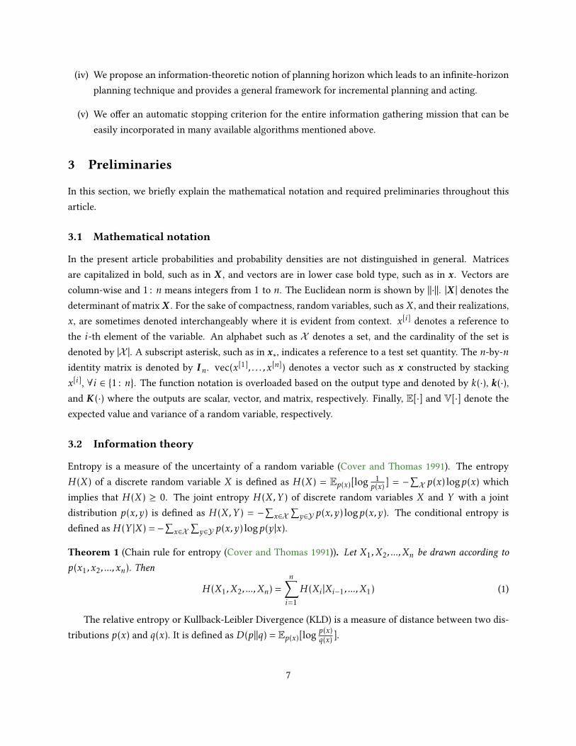
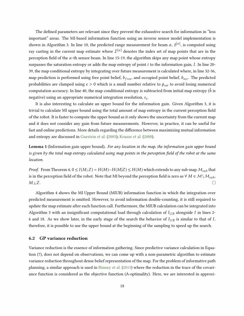
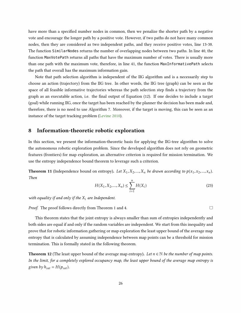
Figure 1: The abstract system for robotic information gathering. The three important questions that we try to answer in thiswork are asked (Q1-Q3). Note that the diagram is conceptual and, in practice, dierent modules can share many attributes andmethods such as parameters and sensor models. The replanning problem is not studied in this work, that is the robot remainscommited to the planned action until it enters the planning state again.

(vi) We provide results in batch and incremental experiments as well as in publicly available roboticdatasets and discuss potential applications of the developed algorithms.

Figure 1 shows a conceptual illustration of the problem studied in this article. The three questions thatwe try to address are: Q1) When to terminate the entire information gathering mission? Q2) When to stopplanning by automatically detecting the convergence of the planner, i.e. planning and acting incremen-tally? And Q3) How to incorporate the uncertainty of the perception system into the planner?

This article is organized as follows. In the next section, the related work is discussed. Section 3 includesrequired preliminaries. In Section 4, we present the problem denition and highlight the dierences be-tween RIG and IIG algorithms. We also explain RIG algorithms to establish the required basis. In Section 5,we present the novel IIG algorithm. In Section 6, we propose two information functions that approximatethe information quality of nodes and trajectories of the associated motion planning problem. In Section 7,the problem of path extraction and selection is explained, and a heuristic algorithm is proposed to solvethe problem. Section 8 presents the proof for an information-theoretic automatic stopping criterion forexploration and information gathering missions. In Section 9, we present an extensive evaluation of theproposed strategies including a comparison with relevant techniques in the literature. A lake monitor-ing scenario based on a publically available dataset is also presented together with a discussion on thelimitations of this work. Finally, Section 10 concludes the article and discusses possible extensions of theproposed algorithms as future work.

4

2 Related work

Motion planning algorithms (Latombe 1991; LaValle 2006) construct a broad area of research in the roboticcommunity. In the presence of uncertainty, where the state is not fully observable, measurements and ac-tions are stochastic. The sequential decision-making under uncertainty, in the most general form, can beformulated as a Partially Observable Markov Decision Processes (POMDP) or optimal control with imper-fect state information (Astrom 1965; Smallwood and Sondik 1973; Bertsekas 1995; Kaelbling et al. 1998).Unfortunately, when the problem is formulated using a dense belief representation, a general purposePOMDP solver is not a practical choice (Binney et al. 2013).

The sampling-based motion planning algorithms (Horsch et al. 1994; Kavraki et al. 1996; LaValle andKuner 2001; Bry and Roy 2011; Karaman and Frazzoli 2011; Lan and Schwager 2013) have proven suc-cessful applications in robotics. An interesting case is where the environment is fully observable (knownmap) and the objective is to make sequential decisions under motion and measurement uncertainty. Thisproblem is also known as active localization; for a recent technique to solve such a problem see Agha-mohammadi et al. (2014, and references therein). A closely related term that is used in the literature isbelief space planning (Kurniawati et al. 2008; Huynh and Roy 2009; Prentice and Roy 2009; Platt Jr et al. 2010;

Kurniawati et al. 2011; Van Den Berg et al. 2011; Bry and Roy 2011; Valencia et al. 2013). In this series of works,the assumption of a known map can be relaxed and the environment is often represented using a set of fea-tures. The objective is to nd a trajectory that minimizes the state uncertainty (the total cost) with respectto a xed or variable (and bounded) planning horizon that can be set according to the budget (Indelmanet al. 2015).

In the context of feature-based representation of the environment, planning actions for SimultaneousLocalization And Mapping (SLAM) using Model Predictive Control (MPC) is studied in Leung et al. (2006a).To enable the robot to explore, a set of “attractors” are dened to resemble informative regions for explo-ration. In particular, it is concluded as expected that a multi-step (three steps) look-ahead MPC planner out-performs the greedy approach. In Atanasov et al. (2014), assuming the sensor dynamics is linear-Gaussian,the stochastic optimal control problem is reduced to a deterministic optimal control problem which can besolved oine. The deterministic nature of the problem has been exploited to solve it using forward valueiteration (Bertsekas 1995; Le Ny and Pappas 2009); furthermore, it is shown that the proposed solution,namely reduced value iteration, has a lower computational complexity than that of forward value itera-tion and its performance is better than the greedy policy. The work is also extended from a single robotto decentralized active information acquisition, and using attractors as dummy exploration landmarks, i.e.frontiers, it has been successfully applied to the active SLAM problem (Atanasov et al. 2015).

Another approach to study the problem of robotic navigation under uncertainty, is known as infor-mative motion planning or robotic information gathering (Leung et al. 2006b; Singh et al. 2009; Levine2010; Binney and Sukhatme 2012; Binney et al. 2013; Hollinger and Sukhatme 2013, 2014; Atanasov 2015).Rapidly-exploring information gathering (Hollinger and Sukhatme 2014), is a technique that solves theproblem of informative motion planning using incremental sampling from the workspace and by partial

5

ordering of nodes builds a graph that contains informative trajectories.In the problem we study in this article, the state variables consist of the robot trajectory and a dense map

of the environment. We build on rapidly-exploring information gathering technique by considering boththe robot pose and the map being partially observable. We also develop an information-theoretic criterionfor the convergence of the search which allows us to perform online robotic exploration in unknownenvironments. The Rapidly-exploring Adaptive Search and Classication (ReASC) (Hollinger 2015) alsoimproves on the rapidly-exploring information gathering by allowing for real-time optimization of searchand classication objective functions. However, ReASC relies on discrete target locations and, similarto Platt Jr et al. (2010), resorts to the maximum likelihood assumption for future observations.

The technique reported in Charrow et al. (2015b,a) is closely related to this work but assumes that therobot poses are known, i.e. fully observable, to solve the problem of information gathering for occupancymapping with the help of geometric frontiers (Yamauchi 1997; Ström et al. 2015). The computationalperformance of the information gain estimation is increased by using Cauchy-Schwarz Quadratic MutualInformation (CSQMI). It is shown that the behavior of CSQMI is similar to that of mutual informationwhile it can be computed faster (Charrow 2015, Subsection 6.2.2 and Figure 6.1). It is argued in Charrowet al. (2015a, Subsection V.C) that: “It is interesting that the human operator stopped once they believed they

had obtained a low uncertainty map and that all autonomous approaches continue reducing the map’s entropy

beyond this point, as they continue until no frontiers are left. However, the nal maps are qualitatively hard

to dierentiate, suggesting a better termination condition is needed.” We agree with this argument and relaxsuch a constraint by exploiting a sampling-based planning strategy to calculate the cost and informationgain while searching for traversable paths in the entire space. We also prove an information-theoreticautomatic stopping criterion for the entire mission which can alleviate this issue. In Subsection 9.3, weconduct robotic exploration experiments to show the eectiveness of the proposed termination condition.We show that the proposed condition enables the robot to produce comparable results while collectingless measurements, but sucient information for the inference.

In particular, the main features of this work that dierentiate the present approach from the literaturementioned above can be summarized as follows.

(i) We allow for dense belief representations. Therefore, we incorporate full state uncertainty, i.e. therobot pose and the map, into the planning process. As a result, the robot behavior has a strongcorrelation with its perception uncertainty.

(ii) We take into account all possible future observations and do not resort to maximum likelihoodassumptions. Therefore, the randomness of future observations is addressed.

(iii) We take into account both cost and information gain. The cost is included through a measure ofdistance, and the information gain quanties the sensing quality and acting uncertainty. Therefore,the planning algorithm runs with respect to available sensing resources and acting limitations.

6

(iv) We propose an information-theoretic notion of planning horizon which leads to an innite-horizonplanning technique and provides a general framework for incremental planning and acting.

(v) We oer an automatic stopping criterion for the entire information gathering mission that can beeasily incorporated in many available algorithms mentioned above.

3 Preliminaries

In this section, we briey explain the mathematical notation and required preliminaries throughout thisarticle.

3.1 Mathematical notation

In the present article probabilities and probability densities are not distinguished in general. Matricesare capitalized in bold, such as in X , and vectors are in lower case bold type, such as in x. Vectors arecolumn-wise and 1: n means integers from 1 to n. The Euclidean norm is shown by ‖·‖. |X | denotes thedeterminant of matrixX . For the sake of compactness, random variables, such as X, and their realizations,x, are sometimes denoted interchangeably where it is evident from context. x[i] denotes a reference tothe i-th element of the variable. An alphabet such as X denotes a set, and the cardinality of the set isdenoted by |X |. A subscript asterisk, such as in x∗, indicates a reference to a test set quantity. The n-by-nidentity matrix is denoted by In. vec(x[1], . . . ,x[n]) denotes a vector such as x constructed by stackingx[i], ∀i ∈ 1: n. The function notation is overloaded based on the output type and denoted by k(·), k(·),and K(·) where the outputs are scalar, vector, and matrix, respectively. Finally, E[·] and V[·] denote theexpected value and variance of a random variable, respectively.

3.2 Information theory

Entropy is a measure of the uncertainty of a random variable (Cover and Thomas 1991). The entropyH(X) of a discrete random variable X is dened as H(X) = Ep(x)[log 1

p(x) ] = −∑X p(x) logp(x) which

implies that H(X) ≥ 0. The joint entropy H(X,Y ) of discrete random variables X and Y with a jointdistribution p(x,y) is dened as H(X,Y ) = −

∑x∈X

∑y∈Y p(x,y) logp(x,y). The conditional entropy is

dened as H(Y |X) = −∑x∈X

∑y∈Y p(x,y) logp(y|x).

Theorem 1 (Chain rule for entropy (Cover and Thomas 1991)). Let X1,X2, ...,Xn be drawn according to

p(x1,x2, ...,xn). Then

H(X1,X2, ...,Xn) =n∑i=1

H(Xi |Xi−1, ...,X1) (1)

The relative entropy or Kullback-Leibler Divergence (KLD) is a measure of distance between two dis-tributions p(x) and q(x). It is dened as D(p||q) = Ep(x)[log

p(x)q(x) ].

7

Theorem 2 (Information inequality (Cover and Thomas 1991)). Let X be a discrete random variable. Let

p(x) and q(x) be two probability mass functions. Then

D(p||q) ≥ 0 (2)

with equality if and only if p(x) = q(x) ∀ x.

The mutual information (MI), I(X;Y ) =D(p(x,y)||p(x)p(y)) =H(X)−H(X |Y ), is the reduction in theuncertainty of one random variable due to the knowledge of the other.

Corollary 3 (Nonnegativity of mutual information). For any two random variables X and Y ,

I(X;Y ) ≥ 0 (3)

with equality if and only if X and Y are independent.

Proof. I(X;Y ) =D(p(x,y)||p(x)p(y)) ≥ 0, with equality if and only if p(x,y) = p(x)p(y).

Some immediate consequences of the provided denitions are as follows.

Theorem 4 (Conditioning reduces entropy). For any two random variables X and Y ,

H(X |Y ) ≤H(X) (4)

with equality if and only if X and Y are independent.

Proof. 0 ≤ I(X;Y ) =H(X)−H(X |Y ).

We now dene the equivalent of the functions mentioned above for probability density functions. LetX be a continuous random variable whose support set is S . Let p(x) be the probability density functionfor X. The dierential entropy h(X) of X is dened as h(X) = −

∫S p(x) logp(x)dx. Let X and Y be contin-

uous random variables that have a joint probability density function p(x,y). The conditional dierentialentropy h(X |Y ) is dened as h(X |Y ) = −

∫p(x,y) logp(x|y)dxdy. The relative entropy (KLD) between two

probability density functions p and q is dened asD(p||q) =∫p log pq . The mutual information I(X;Y ) be-

tween two continuous random variables X and Y with joint probability density function p(x,y) is denedas I(X;Y ) =

∫p(x,y) log p(x,y)

p(x)p(y)dxdy.

3.3 Submodular functions

A set function f is said to be submodular if ∀A ⊆ B ⊆ S and ∀s ∈ S\B, thenf (A∪ s)− f (A) ≥ f (B ∪ s)− f (B). Intuitively, this can be explained as: by adding observations toa smaller set, we gain more information. The function f has diminishing return. It is normalized iff (∅) = 0 and it is monotone if f (A) ≤ f (B). The mutual information is normalized, approximatelymonotone, and submodular (Krause et al. 2008).

8

3.4 Gaussian processes

Gaussian Processes (GPs) are non-parametric Bayesian regression techniques that employ statistical in-ference to learn dependencies between points in a data set (Rasmussen and Williams 2006). The jointdistribution of the observed target values, y, and the function values (the latent variable), f ∗, at the querypoints can be written as yf ∗

∼N (0,

K(X ,X) + σ2n In K(X ,X ∗)

K(X ∗,X) K(X ∗,X ∗)

) (5)

where X is the d × n design matrix of aggregated input vectors x, X ∗ is a d × n∗ query points ma-trix, K(·, ·) is the GP covariance matrix, and σ2

n is the variance of the observation noise which isassumed to have an independent and identically distributed (i.i.d.) Gaussian distribution. Dene atraining set D = (x[i], y[i]) | i = 1: n. The predictive conditional distribution for a single query pointf∗|D,x∗ ∼N (E[f∗],V[f∗]) can be derived as

µ = E[f∗] = k(X ,x∗)T [K(X ,X) + σ2n In]

−1y (6)

σ = V[f∗] = k(x∗,x∗)−k(X ,x∗)T [K(X ,X) + σ2n In]

−1k(X ,x∗) (7)

The hyperparameters of the covariance and mean function, θ, can be computed by minimization ofthe negative log of the marginal likelihood (NLML) function.

logp(y|X ,θ) = −12yT (K(X ,X) + σ2

n In)−1y − 1

2log |K(X ,X) + σ2

n In| −n2log2π (8)

3.4.1 Covariance function

Covariance functions are the main part of any GPs. We dene a covariance function using the kerneldenition as follows.

Denition 1 (Covariance function). Let x ∈ X and x′ ∈ X be a pair of inputs for a function k : X ×X → Rknown as kernel. A kernel is called a covariance function, as the case in Gaussian processes, if it is sym-metric, k(x,x′) = k(x′ ,x), and positive semidenite:∫

k(x,x′)f (x)f (x′)dµ(x)dµ(x′) ≥ 0 (9)

for all f ∈ L2(X ,µ).

Given a set of input points x[i]|i = 1 : n, a covariance matrix can be constructed usingK[i,j] = k(x[i],x[j]) as its entries.

9

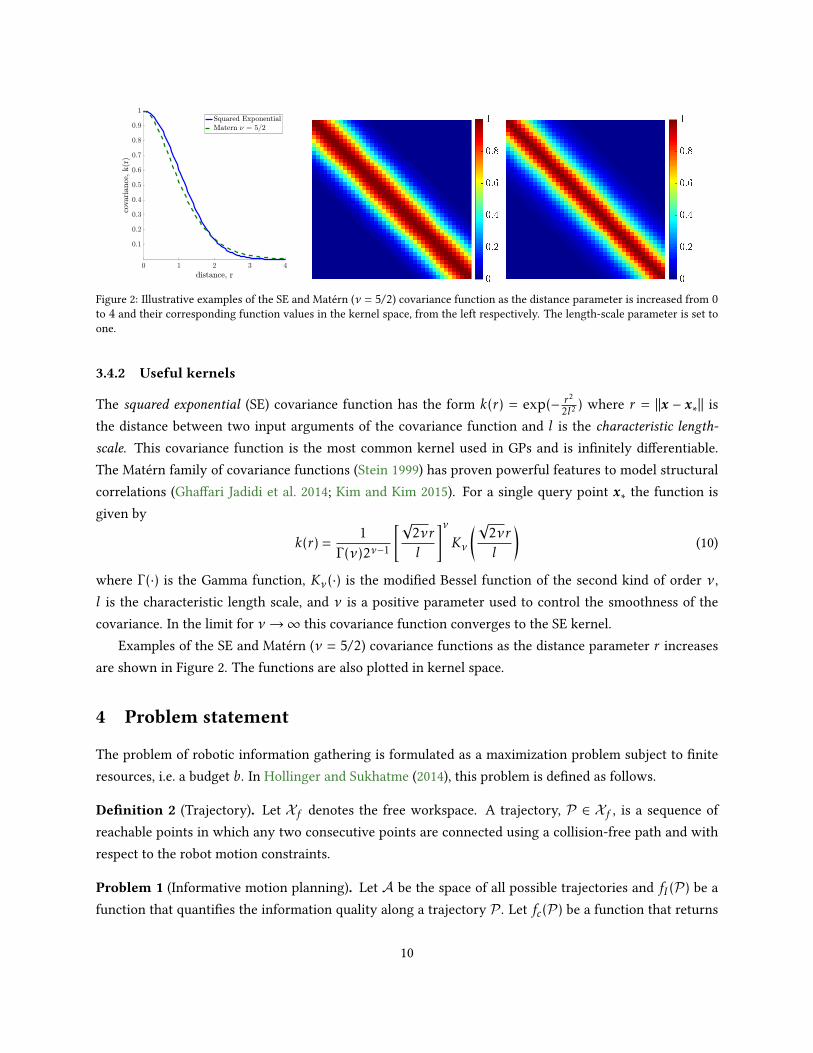
Figure 2: Illustrative examples of the SE and Matérn (ν = 5/2) covariance function as the distance parameter is increased from 0to 4 and their corresponding function values in the kernel space, from the left respectively. The length-scale parameter is set toone.

3.4.2 Useful kernels

The squared exponential (SE) covariance function has the form k(r) = exp(− r22l2 ) where r = ‖x − x∗‖ isthe distance between two input arguments of the covariance function and l is the characteristic length-

scale. This covariance function is the most common kernel used in GPs and is innitely dierentiable.The Matérn family of covariance functions (Stein 1999) has proven powerful features to model structuralcorrelations (Ghaari Jadidi et al. 2014; Kim and Kim 2015). For a single query point x∗ the function isgiven by

k(r) =1

Γ (ν)2ν−1

[√2νrl

]νKν

(√2νrl

)(10)

where Γ (·) is the Gamma function, Kν(·) is the modied Bessel function of the second kind of order ν,l is the characteristic length scale, and ν is a positive parameter used to control the smoothness of thecovariance. In the limit for ν→∞ this covariance function converges to the SE kernel.

Examples of the SE and Matérn (ν = 5/2) covariance functions as the distance parameter r increasesare shown in Figure 2. The functions are also plotted in kernel space.

4 Problem statement

The problem of robotic information gathering is formulated as a maximization problem subject to niteresources, i.e. a budget b. In Hollinger and Sukhatme (2014), this problem is dened as follows.

Denition 2 (Trajectory). Let Xf denotes the free workspace. A trajectory, P ∈ Xf , is a sequence ofreachable points in which any two consecutive points are connected using a collision-free path and withrespect to the robot motion constraints.

Problem 1 (Informative motion planning). Let A be the space of all possible trajectories and fI (P ) be afunction that quanties the information quality along a trajectory P . Let fc(P ) be a function that returns

10

the cost associated with trajectory P . Given the available budget b, the problem can be formulated asfollows.

P ∗ = argmaxP∈A

fI (P ) s.t. fc(P ) ≤ b (11)

Now we express the assumptions in RIG algorithms.

Assumption 5. The cost function fc(P ) is strictly positive, monotonically increasing, bounded, and ad-ditive such as distance and energy.

Remark 1. The information function fI (P ) can be modular, time-varying modular, or submodular.

The information function assumption follows from Hollinger and Sukhatme (2014), even though wefocus our attention on the submodular class of information functions as the information gathered at anyfuture time during navigation depends on prior robot trajectories. Another reason to consider submodularinformation functions is to avoid information “double-counting”. This allows us to develop an information-theoretic convergence criterion for RIG/IIG as the amount of available information remains bounded. Thefollowing assumptions are directly from Hollinger and Sukhatme (2014) which in turn are equivalent oradapted from Bry and Roy (2011); Karaman and Frazzoli (2011). The Steer function used in Assumption 6extends nodes towards newly sampled points.

Assumption 6. Let xa, xb, and xc ∈ Xf be three points within radius ∆ of each other. Let the trajec-tory e1 be generated by Steer(xa,xc,∆), e2 be generated by Steer(xa,xb,∆), and e3 be generated bySteer(xb,xc,∆). If xb ∈ e1, then the concatenated trajectory e2 + e3 must be equal to e1 and have equalcost and information.

This assumption is required as in the limit drawn samples are innitely close together, and the Steerfunction, cost, and information need to be consistent for any intermediate point.

Assumption 7. There exists a constant r ∈ R>0 such that for any point xa ∈ Xf there exists an xb ∈ Xf ,such that 1) the ball of radius r centered at xa lies insideXf and 2) xa lies inside the ball of radius r centeredat xb.

This assumption ensures that there is enough free space near any point for extension of the graph.Violation of this assumption in practice can lead to failure of the algorithm to nd a path.

Assumption 8 (Uniform sampling). 2 Points returned by the sampling function sample are i.i.d. anddrawn from a uniform distribution.

2Results extend naturally to any absolutely continuous distribution with density bounded away from zero on workspaceX (Karaman and Frazzoli 2011).

11

4.1 Incremental informative motion planning

Now we dene the problem of incremental informative motion planning as follows.

Problem 2 (Incremental informative motion planning). Let s0:ts ∈ S be the current estimate of the state upto time ts. Let At be the space of all possible trajectories at time t and fI (Pt) be a function that quantiesthe information quality along a trajectory Pt . Let fc(Pt) be a function that returns the cost associated withtrajectory Pt . Given the available budget bt , the problem can be formulated as follows.

P ∗t =argmaxPt∈At

fI (Pt) ∀ t > ts

s.t. fc(Pt) ≤ bt and S = s0:ts (12)

Remark 2. The state S can include the representation of the environment (map), the robot trajectory,and possibly any other variables dened in the state vector. In general, the information function fI (Pt) isresponsible for incorporating the state uncertainty in the information gain calculations.

Remark 3. In practice we solve the problem incrementally and use a planning horizon T > ts that in thelimit goes to∞.

The main dierence between Problem 1 and Problem 2 is that in the latter the robot does not have thefull knowledge of the environment a priori. Therefore Problem 2 is not only the problem of informationgathering but also planning for estimation as the robot needs to infer the map (and in general its pose inthe SLAM problem) sequentially. Note that we do not impose any assumptions on the observability of therobot pose and the map; therefore, they can be partially observable as is the case in POMDPs.

The aforementioned problems are both in their oine (nonadaptive) and online (adaptive) forms NP-hard (Singh et al. 2009). We build our proposed incremental information gathering algorithm on top ofthe RIG to solve the interesting problem of autonomous robotic exploration in unknown environments.Furthermore, since the ultimate goal is online applications, we only consider the RIG-tree variant to beextended for sequential planning. This conclusion stems from extensive comparisons of RIG variantsprovided in Hollinger and Sukhatme (2014). However, we acknowledge that the RIG-graph is an interestingcase to consider as under a partial ordering assumption it is asymptotically optimal.

4.2 RIG algorithms

The sampling-based RIG algorithms nd a trajectory that maximizes an information quality metric withrespect to a pre-specied budget constraint (Hollinger and Sukhatme 2014). The RIG is based on RRT*,RRG, and PRM* (Karaman and Frazzoli 2011) and borrow the notion of informative path planning frombranch and bound optimization (Binney and Sukhatme 2012). Algorithm 1 shows the RIG-tree algorithm.The functions that are used in the algorithm are explained as follows.

12

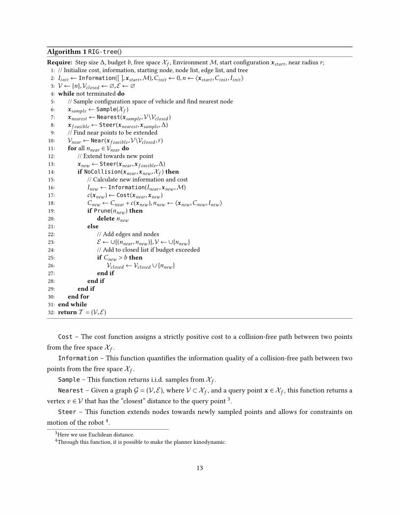
Algorithm 1 RIG-tree()Require: Step size ∆, budget b, free space Xf , EnvironmentM, start conguration xstart , near radius r;

1: // Initialize cost, information, starting node, node list, edge list, and tree2: Iinit← Information([ ],xstart ,M),Cinit← 0,n← 〈xstart ,Cinit , Iinit〉3: V ← n,Vclosed ←∅,E ←∅4: while not terminated do5: // Sample conguration space of vehicle and nd nearest node6: xsample← Sample(Xf )7: xnearest← Nearest(xsample,V\Vclosed)8: xf easible← Steer(xnearest ,xsample,∆)9: // Find near points to be extended

10: Vnear ← Near(xf easible,V\Vclosed , r)11: for all nnear ∈ Vnear do12: // Extend towards new point13: xnew← Steer(xnear ,xf easible,∆)14: if NoCollision(xnear ,xnew,Xf ) then15: // Calculate new information and cost16: Inew← Information(Inear ,xnew,M)17: c(xnew)← Cost(xnear ,xnew)18: Cnew← Cnear + c(xnew),nnew← 〈xnew,Cnew, Inew〉19: if Prune(nnew) then20: delete nnew21: else22: // Add edges and nodes23: E ← ∪(nnear ,nnew),V ←∪nnew24: // Add to closed list if budget exceeded25: if Cnew > b then26: Vclosed ←Vclosed ∪ nnew27: end if28: end if29: end if30: end for31: end while32: return T = (V ,E)

Cost – The cost function assigns a strictly positive cost to a collision-free path between two pointsfrom the free space Xf .

Information – This function quanties the information quality of a collision-free path between twopoints from the free space Xf .

Sample – This function returns i.i.d. samples from Xf .Nearest – Given a graph G = (V ,E), where V ⊂ Xf , and a query point x ∈ Xf , this function returns a

vertex v ∈ V that has the “closest” distance to the query point 3.Steer – This function extends nodes towards newly sampled points and allows for constraints on

motion of the robot 4.3Here we use Euclidean distance.4Through this function, it is possible to make the planner kinodynamic.

13

Near – Given a graph G = (V ,E), where V ⊂ Xf , a query point x ∈ Xf , and a positive real numberr ∈ R>0, this function returns a set of vertices Vnear ⊆ V that are contained in a ball of radius r centered atx.

NoCollision – Given two points xa,xb ∈ Xf , this functions returns true if the line segment betweenxa and xb is collision-free and false otherwise.

Prune – This function implements a pruning strategy to remove nodes that are not “promising”. Thiscan be achieved through dening a partial ordering for co-located nodes.

In line 2-3 the algorithm initializes the starting node of the graph (tree). In line 6-8, a sample pointfrom workspace X is drawn and is converted to a feasible point, from its nearest neighbor in the graph.Line 10 extracts all nodes from the graph that are within radius r of the feasible point. These nodes arecandidates for extending the graph, and each node is converted to a new node using the Steer function inline 13. In line 14-18, if there exists a collision free path between the candidate node and the new node, theinformation gain and cost of the new node are evaluated. In line 19-26, if the new node does not satisfya partial ordering condition it is pruned, otherwise it is added to the graph. Furthermore, the algorithmchecks for the budget constraint violation. The output is a graph that contains a subset of traversable pathswith maximum information gain.

4.3 System dynamics

The equation of motion of the robot is governed by the nonlinear partially observable equation as follows.

x−t+1 = f (xt ,ut ,wt) wt ∼N (0,Qt) (13)

moreover, with appropriate linearization at the current state estimate, we can predict the state covariancematrix as

Σ−t+1 = F tΣtFTt +W tQtW

Tt (14)

where F t =∂f∂x |xt ,ut and W t =

∂f∂w |xt ,ut are the Jacobian matrices calculated with respect to x and w,

respectively.

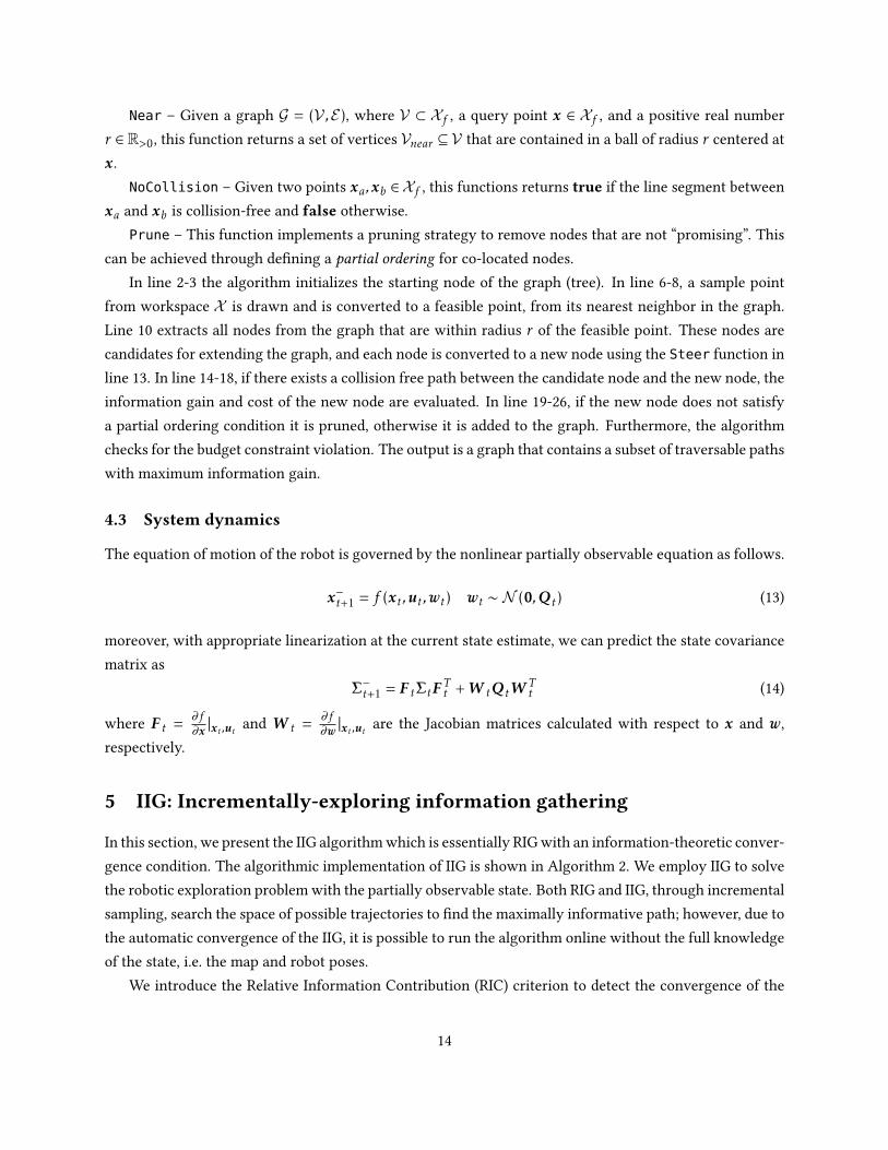
5 IIG: Incrementally-exploring information gathering

In this section, we present the IIG algorithm which is essentially RIG with an information-theoretic conver-gence condition. The algorithmic implementation of IIG is shown in Algorithm 2. We employ IIG to solvethe robotic exploration problem with the partially observable state. Both RIG and IIG, through incrementalsampling, search the space of possible trajectories to nd the maximally informative path; however, due tothe automatic convergence of the IIG, it is possible to run the algorithm online without the full knowledgeof the state, i.e. the map and robot poses.

We introduce the Relative Information Contribution (RIC) criterion to detect the convergence of the

14

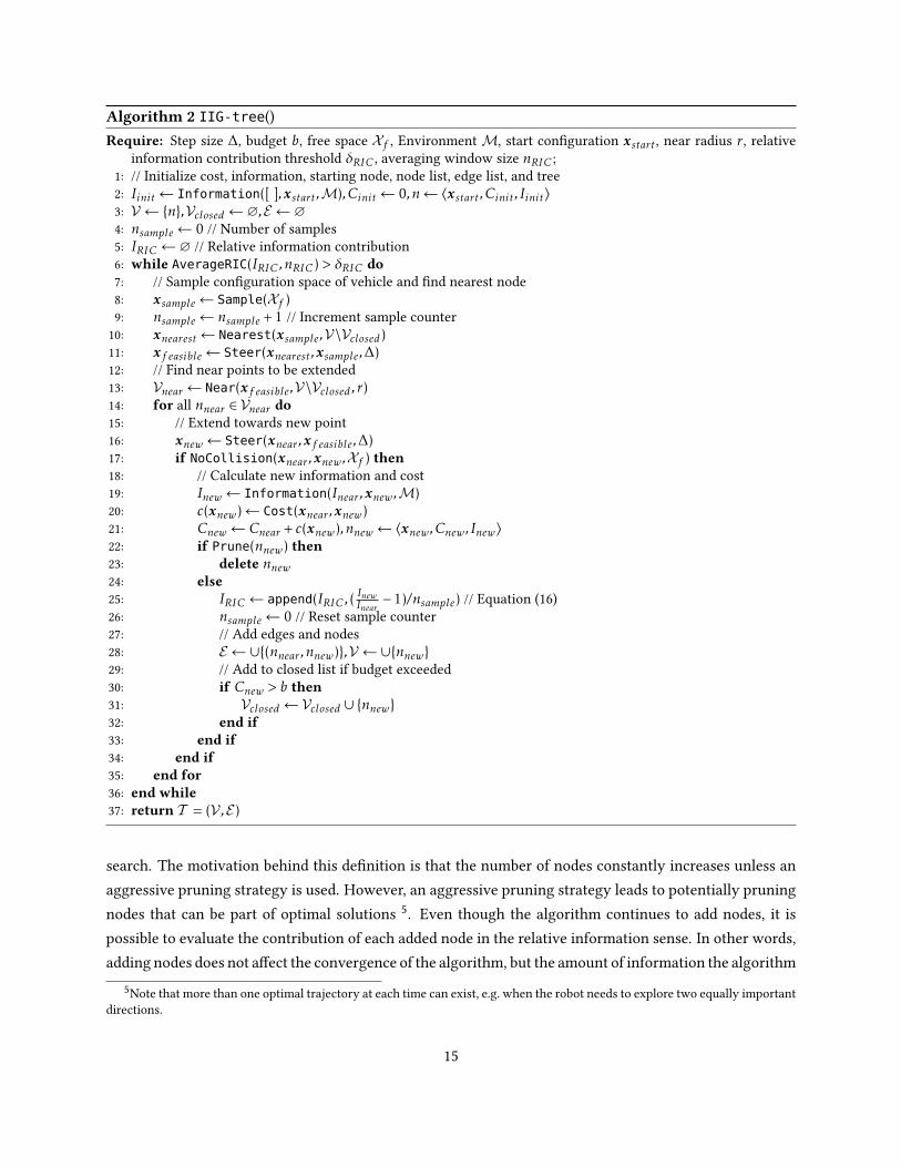
Algorithm 2 IIG-tree()Require: Step size ∆, budget b, free space Xf , EnvironmentM, start conguration xstart , near radius r , relative

information contribution threshold δRIC , averaging window size nRIC ;1: // Initialize cost, information, starting node, node list, edge list, and tree2: Iinit← Information([ ],xstart ,M),Cinit← 0,n← 〈xstart ,Cinit , Iinit〉3: V ← n,Vclosed ←∅,E ←∅4: nsample← 0 // Number of samples5: IRIC ←∅ // Relative information contribution6: while AverageRIC(IRIC ,nRIC) > δRIC do7: // Sample conguration space of vehicle and nd nearest node8: xsample← Sample(Xf )9: nsample← nsample +1 // Increment sample counter

10: xnearest← Nearest(xsample,V\Vclosed)11: xf easible← Steer(xnearest ,xsample,∆)12: // Find near points to be extended13: Vnear ← Near(xf easible,V\Vclosed , r)14: for all nnear ∈ Vnear do15: // Extend towards new point16: xnew← Steer(xnear ,xf easible,∆)17: if NoCollision(xnear ,xnew,Xf ) then18: // Calculate new information and cost19: Inew← Information(Inear ,xnew,M)20: c(xnew)← Cost(xnear ,xnew)21: Cnew← Cnear + c(xnew),nnew← 〈xnew,Cnew, Inew〉22: if Prune(nnew) then23: delete nnew24: else25: IRIC ← append(IRIC , (

InewInear− 1)/nsample) // Equation (16)

26: nsample← 0 // Reset sample counter27: // Add edges and nodes28: E ← ∪(nnear ,nnew),V ←∪nnew29: // Add to closed list if budget exceeded30: if Cnew > b then31: Vclosed ←Vclosed ∪ nnew32: end if33: end if34: end if35: end for36: end while37: return T = (V ,E)

search. The motivation behind this denition is that the number of nodes constantly increases unless anaggressive pruning strategy is used. However, an aggressive pruning strategy leads to potentially pruningnodes that can be part of optimal solutions 5. Even though the algorithm continues to add nodes, it ispossible to evaluate the contribution of each added node in the relative information sense. In other words,adding nodes does not aect the convergence of the algorithm, but the amount of information the algorithm

5Note that more than one optimal trajectory at each time can exist, e.g. when the robot needs to explore two equally importantdirections.

15

can collect by continuing the search. We dene the RIC of a node as follows.

Denition 3 (Relative Information Contribution). In Algorithm 2, let xnew ∈ Xf be a reachable pointthrough a neighboring node nnear ∈ V returned by the function Near(). Let Inew and Inear be the informa-tion values of their corresponding nodes returned by the function Information(). The relative informationcontribution of node nnew is dened as

RIC ,InewInear

− 1 (15)

Equation (15) is conceptually important as it denes the amount of information gain relative to aneighboring point in the IIG graph. In practice, the number of samples it takes before the algorithm nds anew node becomes important. Thus we dene penalized relative information contribution that is computedin line 25.

Denition 4 (Penalized Relative Information Contribution). Let RIC be the relative information contri-bution computed using Equation (15). Let nsample be the number of samples it takes to nd the node nnew.The penalized relative information contribution is dened as

IRIC ,RICnsample

(16)

An appealing property of IRIC is that it is non-dimensional, and it does not depend on the actual cal-culation/approximation of the information values. In practice, as long as the information function satisesthe RIG/IIG requirements, using the following condition, IIG algorithm converges. Let δRIC be a thresholdthat is used to detect the convergence of the algorithm. Through averaging IRIC values over a window ofsize nRIC , we ensure that continuing the search will not add any signicant amount of information to theIIG graph. In Algorithm 2, this condition is shown in line 6 by function AverageRIC.

Remark 4. In Algorithm 2, δRIC sets the planning horizon from the information gathering point of view.Through using smaller values of δRIC the planner can reach further points in both spatial and belief space.In other words, if δRIC → 0, then T →∞.

6 Information functions algorithms

We propose two classes of algorithms to approximate the information gain at any sampled point fromthe free workspace. The information function in RIG/IIG algorithms often causes a bottleneck and com-putationally dominates the other parts. Therefore, even for oine calculations, it is important to haveaccess to functions that, concurrently, are computationally tractable and can capture the essence of in-formation gathering. We emphasize that the information functions are directly related to the employedsensors. However, once the model is provided and incorporated into the estimation/prediction algorithms,the information-theoretic aspects of the provided algorithms remain the same.

16

The information functions that are proposed are dierent in nature. First, we discuss MI-based infor-mation functions whose calculations explicitly depend on the probabilistic sensor model. We provide avariant of the MI Algorithm in Ghaari Jadidi et al. (2015, 2016) that is developed for range-nder sensorsand based on the beam-based mixture measurement model and the inverse sensor model map predic-tion (Thrun et al. 2005). We also present an algorithm to approximate MI upper bound which reveals themaximum achievable information gain.

Then, we exploit the property of GPs to approximate the information gain. In Equation (7), the vari-ance calculation does not explicitly depend on the target vector (measurements) realization. In this case,as long as the underlying process is modeled as GPs, the information gain can be calculated using priorand posterior variances which removes the need for relying on a specic sensor model and calculatingthe expectation over future measurements. However, note that the hyperparameters of the covariancefunctions are learned using the training set which contains measurements; therefore, the knowledge ofunderlying process and measurements is incorporated into the GP through its hyperparameters. Oncewe established GP Variance Reduction (GPVR) algorithm, we then use the expected kernel notion (Ghaf-fari Jadidi et al. 2017) to propagate pose uncertainty into the covariance function resulting in UncertainGP Variance Reduction (UGPVR) algorithm. In particular, these two information functions are interestingfor the following reasons:

(i) Unlike MI-based (direct information gain calculation), they are non-parametric.

(ii) GPVR-based information functions provide a systematic way to incorporate input (state) uncertaintyinto information gathering frameworks.

(iii) In the case of incomplete knowledge about the quantity of interest in an unknown environment,they allow for active learning 6.

6.1 Mutual information

To calculate MI without information “double-counting” we need to update the map after every measure-ment prediction. It is possible to perform map prediction using a forward or inverse sensor model (Thrunet al. 2005). Typically using an inverse sensor model results in simpler calculations. We rst dene tworequired parameters in the proposed algorithm as follows.

Denition 5 (Map saturation probability). The probability that the robot is completely condent aboutthe occupancy status of a point is dened as psat .

Denition 6 (Map saturation entropy). The entropy of a point from a map whose occupancy probabilityis psat , is dened as hsat ,H(psat).

6Although this is one of the most interesting aspects of GPVR-based information functions, it is beyond the scope of thisarticle, and we leave it as a possible extension of this work.

17

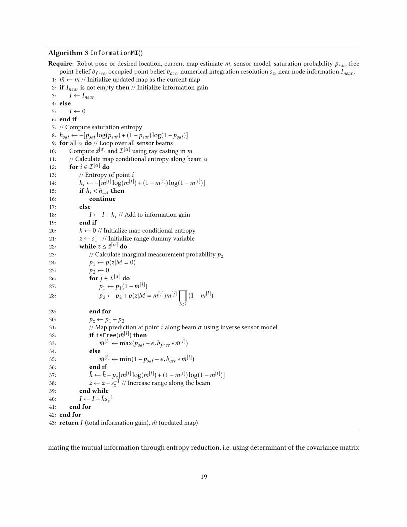
The dened parameters are relevant since they prevent the exhaustive search for information in “lessimportant” areas. The MI-based information function using an inverse sensor model implementation isshown in Algorithm 3. In line 10, the predicted range measurement for beam α, z[α], is computed usingray casting in the current map estimate where I [α] denotes the index set of map points that are in theperception eld of the α-th sensor beam. In line 15-19, the algorithm skips any map point whose entropysurpasses the saturation entropy or adds the map entropy of point i to the information gain, I . In line 20-39, the map conditional entropy by integrating over future measurement is calculated where, in line 32-36,map prediction is performed using free point belief, bf ree, and occupied point belief, bocc. The predictedprobabilities are clamped using ε > 0 which is a small number relative to psat to avoid losing numericalcomputation accuracy. In line 40, the map conditional entropy is subtracted from initial map entropy (h isnegative) using an appropriate numerical integration resolution, sz.

It is also interesting to calculate an upper bound for the information gain. Given Algorithm 3, it istrivial to calculate MI upper bound using the total amount of map entropy in the current perception eldof the robot. It is faster to compute the upper bound as it only shows the uncertainty from the current mapand it does not consider any gain from future measurements. However, in practice, it can be useful forfast and online predictions. More details regarding the dierence between maximizing mutual informationand entropy are discussed in Guestrin et al. (2005); Krause et al. (2008).

Lemma 1 (Information gain upper bound). For any location in the map, the information gain upper bound

is given by the total map entropy calculated using map points in the perception eld of the robot at the same

location.

Proof. From Theorem 4, 0 ≤ I(M;Z) =H(M)−H(M |Z) ≤H(M)which extends to any sub-mapMsub thatis in the perception eld of the robot. Note that MI beyond the perception eld is zero as ∀M ∈M\Msub,M⊥Z .

Algorithm 4 shows the MI Upper Bound (MIUB) information function in which the integration overpredicted measurement is omitted. However, to avoid information double-counting, it is still required toupdate the map estimate after each function call. Furthermore, the MIUB calculation can be integrated intoAlgorithm 3 with an insignicant computational load through calculation of IUB alongside I in lines 2-6 and 18. As we show later, in the early stage of the search the behavior of IUB is similar to that of I ,therefore, it is possible to use the upper bound at the beginning of the sampling to speed up the search.

6.2 GP variance reduction

Variance reduction is the essence of information gathering. Since predictive variance calculation in Equa-tion (7), does not depend on observations, we can come up with a non-parametric algorithm to estimatevariance reduction throughout dense belief representation of the map. For the problem of informative pathplanning, a similar approach is used in Binney et al. (2013) where the reduction in the trace of the covari-ance function is considered as the objective function (A-optimality). Here, we are interested in approxi-

18

Algorithm 3 InformationMI()Require: Robot pose or desired location, current map estimate m, sensor model, saturation probability psat , free

point belief bf ree, occupied point belief bocc, numerical integration resolution sz, near node information Inear ;1: m←m // Initialize updated map as the current map2: if Inear is not empty then // Initialize information gain3: I ← Inear4: else5: I ← 06: end if7: // Compute saturation entropy8: hsat←−[psat log(psat) + (1− psat) log(1− psat)]9: for all α do // Loop over all sensor beams

10: Compute z[α] and I [α] using ray casting in m11: // Calculate map conditional entropy along beam α12: for i ∈ I [α] do13: // Entropy of point i14: hi ←−[m[i] log(m[i]) + (1− m[i]) log(1− m[i])]15: if hi < hsat then16: continue17: else18: I ← I + hi // Add to information gain19: end if20: h← 0 // Initialize map conditional entropy21: z← s−1z // Initialize range dummy variable22: while z ≤ z[α] do23: // Calculate marginal measurement probability pz24: p1← p(z|M = 0)25: p2← 026: for j ∈ I [α] do27: p1← p1(1−m[j])28: p2← p2 + p(z|M =m[j])m[j]

∏l<j

(1−m[l])

29: end for30: pz← p1 + p231: // Map prediction at point i along beam α using inverse sensor model32: if isFree(m[i]) then33: m[i]←max(psat − ε,bf ree ∗ m[i])34: else35: m[i]←min(1− psat + ε,bocc ∗ m[i])36: end if37: h← h+ pz[m[i] log(m[i]) + (1− m[i]) log(1− m[i])]38: z← z+ s−1z // Increase range along the beam39: end while40: I ← I + hs−1z41: end for42: end for43: return I (total information gain), m (updated map)

mating the mutual information through entropy reduction, i.e. using determinant of the covariance matrix

19

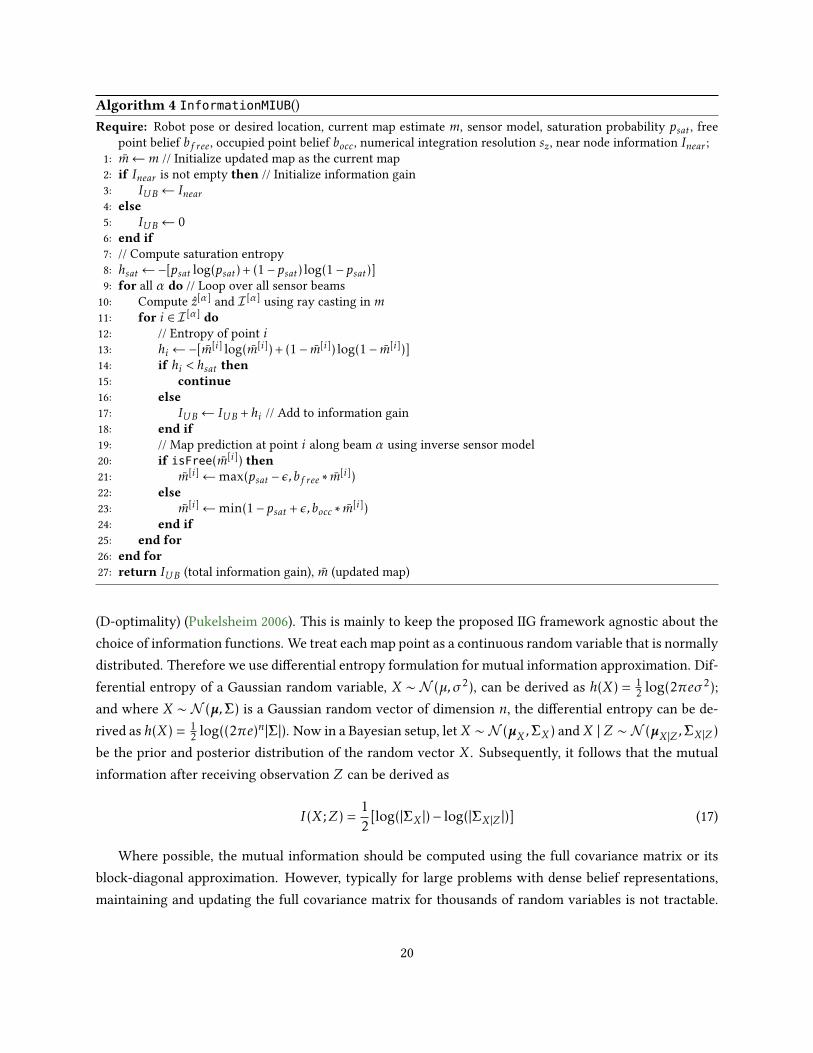
Algorithm 4 InformationMIUB()Require: Robot pose or desired location, current map estimate m, sensor model, saturation probability psat , free

point belief bf ree, occupied point belief bocc, numerical integration resolution sz, near node information Inear ;1: m←m // Initialize updated map as the current map2: if Inear is not empty then // Initialize information gain3: IUB← Inear4: else5: IUB← 06: end if7: // Compute saturation entropy8: hsat←−[psat log(psat) + (1− psat) log(1− psat)]9: for all α do // Loop over all sensor beams

10: Compute z[α] and I [α] using ray casting in m11: for i ∈ I [α] do12: // Entropy of point i13: hi ←−[m[i] log(m[i]) + (1− m[i]) log(1− m[i])]14: if hi < hsat then15: continue16: else17: IUB← IUB + hi // Add to information gain18: end if19: // Map prediction at point i along beam α using inverse sensor model20: if isFree(m[i]) then21: m[i]←max(psat − ε,bf ree ∗ m[i])22: else23: m[i]←min(1− psat + ε,bocc ∗ m[i])24: end if25: end for26: end for27: return IUB (total information gain), m (updated map)

(D-optimality) (Pukelsheim 2006). This is mainly to keep the proposed IIG framework agnostic about thechoice of information functions. We treat each map point as a continuous random variable that is normallydistributed. Therefore we use dierential entropy formulation for mutual information approximation. Dif-ferential entropy of a Gaussian random variable, X ∼N (µ,σ2), can be derived as h(X) = 1

2 log(2πeσ2);

and where X ∼N (µ,Σ) is a Gaussian random vector of dimension n, the dierential entropy can be de-rived as h(X) = 1

2 log((2πe)n|Σ|). Now in a Bayesian setup, letX ∼N (µX ,ΣX) andX | Z ∼N (µX |Z ,ΣX |Z )

be the prior and posterior distribution of the random vector X. Subsequently, it follows that the mutualinformation after receiving observation Z can be derived as

I(X;Z) =12[log(|ΣX |)− log(|ΣX |Z |)] (17)

Where possible, the mutual information should be computed using the full covariance matrix or itsblock-diagonal approximation. However, typically for large problems with dense belief representations,maintaining and updating the full covariance matrix for thousands of random variables is not tractable.

20

Therefore, to approximate the mutual information, we suggest a trade-o approach between the tractabil-ity and accuracy based on the problem at hand. In the following, we propose an approximation of themutual information using the marginalization property of normal distribution. We also discuss the rela-tion of this approximation with the exact mutual information.

Lemma 2 (Marginalization property of normal distribution (Von Mises 1964)). Let x and y be jointly Gaus-sian random vectors xy

∼N (

µxµy , A C

CT B

) (18)

then the marginal distribution of x is

x ∼N (µx,A) (19)

Proposition 9. Let X1,X2, ...,Xn have a multivariate normal distribution with covariance matrix K . The

mutual information between X and observations Z can be approximated as

I(X;Z) =12[n∑i=1

log(σXi )−n∑i=1

log(σXi |Z )] (20)

where σXi and σXi |Z are marginal variances for Xi before and after incorporating observations Z , i.e. prior

and posterior marginal variances.

Proof. Using marginalization property of normal distribution, Lemma 2, for every Xi we have V[Xi] =K[i,i]. Using dierential entropy of Xi , the mutual information for Xi can be written as

I [i](Xi ;Z) =12[log(σXi )− log(σXi |Z )] (21)

and the total mutual information can be calculated as I(X;Z) =∑ni=1 I

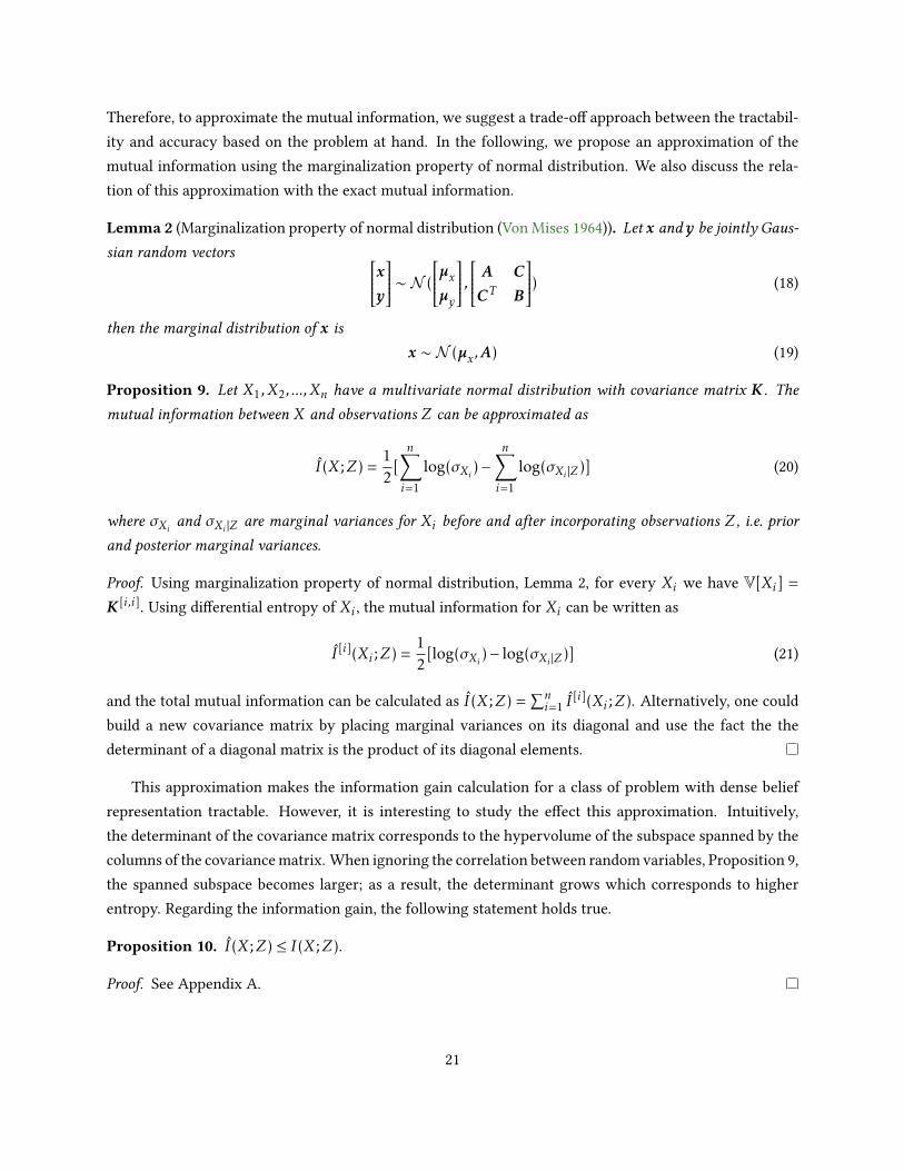
[i](Xi ;Z). Alternatively, one couldbuild a new covariance matrix by placing marginal variances on its diagonal and use the fact the thedeterminant of a diagonal matrix is the product of its diagonal elements.

This approximation makes the information gain calculation for a class of problem with dense beliefrepresentation tractable. However, it is interesting to study the eect this approximation. Intuitively,the determinant of the covariance matrix corresponds to the hypervolume of the subspace spanned by thecolumns of the covariance matrix. When ignoring the correlation between random variables, Proposition 9,the spanned subspace becomes larger; as a result, the determinant grows which corresponds to higherentropy. Regarding the information gain, the following statement holds true.

Proposition 10. I(X;Z) ≤ I(X;Z).

Proof. See Appendix A.

21

Algorithm 5 InformationGPVR()Require: Robot pose or desired location p, current map/state estimate m, covariance function k(·, ·), sensor noise

σ2n , near node information Inear ;

1: σ ← σ // Initialize updated map variance as the current map variance2: if Inear is not empty then // Initialize information gain3: I ← Inear4: else5: I ← 06: end if7: z← Predict future measurements using p and m8: D← Construct training set using z and p9: // Find the corresponding nearest sub-map

10: MD←∅11: for all x ∈ D do12: xnearest← Nearest(x,M)13: MD←MD ∪ xnearest14: end for15: // Calculate self-covariance and cross-covariance matrices16: C←K(X ,X),C∗←K(X ,X ∗) // X ∈ D and X ∗ ∈MD17: // Calculate vector of diagonal variances for test points18: c∗∗← diag(K(X ∗,X ∗))19: L← Cholesky(C + σ2

n I ), V ← L\C∗20: v← c∗∗ − dot(V ,V )T // dot product21: for all i ∈MD do22: σ [i]← ((σ [i])−1 + (v[i])−1)−1 // BCM fusion23: I ← I + log(σ [i])− log(σ [i])24: end for25: return I (total information gain), σ (updated map variance)

Algorithm 5 shows the details of GPVR information function 7. Based on the training points generatedfrom predicted measurement z, a sub-map from the current map estimate using nearest neighbor searchis found, line 7-14. In line 16-20, GP predictive variances, v = vec(v[1], . . . , v[|MD |]), are computed usingcovariance function k(·, ·) with the same hyperparameters learned for the map inference. In line 21-24,using Bayesian Committee Machine (BCM) fusion (Tresp 2000) the predictive marginal posterior varianceis calculated and the information gain is updated consequently 8. BCM combines estimators which weretrained on dierent data sets and is shown to be suitable for incremental map building (Ghaari Jadidiet al. 2016). The Cholesky factorization is the most computationally expensive operation of the algorithm.However, it is possible to exploit a sparse covariance matrix such as the kernel in Melkumyan and Ramos(2009) or use a cut-o distance for the covariance function 9 to speed up the algorithm.

We emphasize that to use GPVR Algorithm, the underlying process needs to be modeled using GPs,i.e. y(x) ∼ GP (fm(x), k(x,x′)) where fm(x) is the GP mean function. Therefore, for any map point we

7The algorithm uses MATLAB-style operations for matrix inversion, Cholesky factorization, and dot product with matrixinputs.

8Note that the constant factor 12 is removed since it does not have any eect in this context.

9The positive semidenite property of the covariance matrix needs to be preserved.

22

havem[i] = y(x[i]∗ ) ∼N (µ[i],σ [i]). Furthermore, construction of the training set, in line 8, is part of the GPmodeling. For the particular case of occupancy mapping using a range-nder sensor see (Ghaari Jadidi2017, Chapter 4). For the case where the robot only receives point measurements at any location, such aswireless signal strength, we explain in Subsection 9.4.

6.3 Uncertain GP variance reduction

Thus far, the developed information functions do not incorporate uncertainties of other state variables thatare jointly distributed with the map (such as the robot pose) in information gain calculation. We denethe modied kernel k as follows.

Denition 7 (Modied kernel). Let k(x,x∗) be a kernel and X ∈ X a random variable that is distributedaccording to a probability distribution function p(x). The modied kernel is dened as its expectation withrespect to p(x), therefore we can write

k = E[k] =∫Ω

kdp (22)

Through replacing the kernel function in Algorithm 5 with the modied kernel we can propagate therobot pose uncertainty in the information gain calculation. Intuitively, under the presence of uncertainty inother state variables that are correlated with the map, the robot does not take greedy actions as the amountof available information calculated using the modied kernel is less than the original case. Therefore, thechosen actions are relatively more conservative. The integration in Equation (22) can be numericallyapproximated using Monte-Carlo or Gauss-Hermite quadrature techniques (Davis and Rabinowitz 1984;Press et al. 1996). In the case of a Gaussian assumption for the robot pose, Gauss-Hermite quadratureprovides a better accuracy and eciency trade-o and is preferred.

Algorithm 6 shows UGPVR information function. The dierence with GPVR is that the input locationis not deterministic, i.e. it is approximated as a normal distribution N (p,Σ), and the covariance functionis replaced by its modied version. Given the initial pose belief, the pose uncertainty propagation on theIIG graph can be performed using the robot motion model, i.e. using Equations (13) and (14).

The UGPVR estimate at most the same amount of mutual information as GPVR. This is because oftaking the expectation of the kernel with respect to the robot pose posterior. If we pick the mode of therobot pose posterior, GPVR only uses that input point for mutual information computation. In contrast,UGPVR averages over all possible values of the robot pose within the support of its distribution. Nowit is clear that having an estimate of the robot pose posterior with long tails (yet exponentially bounded)reduces the mutual information even further due to averaging. Furthermore, if the robot pose is not knownand we have only access to its estimate, ignoring the distribution can lead to overcondent or inconsistentinference/prediction (Ghaari Jadidi et al. 2017, Figure 2).

23

Algorithm 6 InformationUGPVR()Require: Robot pose or desired locationN (p,Σ), current map/state estimatem, modied covariance function k(·, ·),

sensor noise σ2n , near node information Inear ;

1: σ ← σ // Initialize updated map variance as the current map variance2: if Inear is not empty then // Initialize information gain3: I ← Inear4: else5: I ← 06: end if7: z← Predict future measurements using p and m8: D← Construct the training set using z and p9: // Find the corresponding nearest sub-map

10: MD←∅11: for all x ∈ D do12: xnearest← Nearest(x,M)13: MD←MD ∪ xnearest14: end for15: // Calculate self-covariance and cross-covariance matrices using k(·, ·) with respect toN (p,Σ)16: C← K(X ,X),C∗← K(X ,X ∗) // X ∈ D and X ∗ ∈MD17: // Calculate vector of diagonal variances for test points18: c∗∗← diag(K(X ∗,X ∗))19: L← Cholesky(C + σ2

n I ), V ← L\C∗20: v← c∗∗ − dot(V ,V )T // dot product21: for all i ∈MD do22: σ [i]← ((σ [i])−1 + (v[i])−1)−1 // BCM fusion23: I ← I + log(σ [i])− log(σ [i])24: end for25: return I (total information gain), σ (updated map variance)

7 Path extraction and selection

In the absence of articial targets such as frontiers, in general, there is no goal to be found by the planner.IIG searches for traversable paths within the map, and the resulting tree shows feasible trajectories fromthe current robot pose to each leaf node, expanded using the maximum information gathering policy.Therefore, any path in the tree starting from the robot pose to a leaf node is a feasible action. For roboticexploration scenarios, it is not possible to traverse all the available trajectories since, after execution ofone trajectory, new measurements are taken, and the map (and the robot pose) belief is updated; therefore,previous predictions are obsolete, and the robot has to enter the planning state 10. As such, once theRIG/IIG tree is available, next step can be seen as decision-making where the robot selects a trajectoryas an executable action. One possible solution is nding a trajectory in the IIG tree that maximizes theinformation gain.

We provide a heuristic algorithm based on a voting method. Algorithm 7 shows the implementationof the proposed method. The algorithm rst nds all possible paths using a preorder depth rst search,

10Here we assume the robot remains committed to the selected action, i.e. there is no replanning while executing an action.

24

Algorithm 7 PathSelection()Require: RIG/IIG tree T , path similarity ratio sratio;

1: // The path length equals the number of nodes in the path.2: // Find all leaves using depth rst search3: Vleaves← DFSpreorder(T )4: // Find all paths by starting from each leaf and following parent nodes5: Pall ← Paths2root(T ,Vleaves)6: lmax← Find maximum path length in Pall7: lmin← ceil(κlmax) // Minimum path length, 0 < κ < 18: for all P ∈ Pall do9: if length(P ) ≤ lmin then

10: Delete P11: end if12: end for13: np← |Pall | // Number of paths in set Pall14: vote← zeros(np,1)15: // Find longest independent paths16: i← 117: while i ≤ np − 1 do18: j← i +119: while j ≤ np do20: li ← length(Pi), lj ← length(Pj )21: // Find number of common nodes between paths i and j , and the length ratio they share22: lij ← SimilarNodes(Pi ,Pj )/min(li , lj )23: if lij > sratio then24: if li > lj then // Path i is longer25: vote[i]← vote[i] +126: vote[j]← vote[j] − 127: else // Path j is longer28: vote[i]← vote[i] − 129: vote[j]← vote[j] +130: end if31: else // Two independent paths32: vote[i]← vote[i] +133: vote[j]← vote[j] +134: end if35: j← j +136: end while37: i← i +138: end while39: // Find paths with maximum vote and select the maximally informative path40: Pmax← MaxVotePath(Pall ,vote)41: PI ← MaxInformativePath(Pmax)42: return PI

function DFSpreorder, and then removes paths that are shorter than a minimum length (using parameter0 < κ < 1), line 3-12. Note that the path length and the length returned by function length are integers andcorrespond to the number of nodes in the path; consequently, the path length in Algorithm 7 is independentof the actual path scale. Then each path is compared with others using the following strategy. If two paths

25

have more than a specied number nodes in common, then we penalize the shorter path by a negativevote and encourage the longer path by a positive vote. However, if two paths do not have many commonnodes, then they are considered as two independent paths, and they receive positive votes, line 13-38.The function SimilarNodes returns the number of overlapping nodes between two paths. In line 40, thefunction MaxVotePath returns all paths that have the maximum number of votes. There is usually morethan one path with the maximum vote, therefore, in line 41, the function MaxInformativePath selectsthe path that overall has the maximum information gain.

Note that path selection algorithm is independent of the IIG algorithm and is a necessarily step tochoose an action (trajectory) from the IIG tree. In other words, the IIG tree (graph) can be seen as thespace of all feasible informative trajectories whereas the path selection step nds a trajectory from thegraph as an executable action, i.e. the nal output of Equation (12). If one decides to include a target(goal) while running IIG, once the target has been reached by the planner the decision has been made and,therefore, there is no need to use Algorithm 7. Moreover, if the target is moving, this can be seen as aninstance of the target tracking problem (Levine 2010).

8 Information-theoretic robotic exploration

In this section, we present the information-theoretic basis for applying the IIG-tree algorithm to solvethe autonomous robotic exploration problem. Since the developed algorithm does not rely on geometricfeatures (frontiers) for map exploration, an alternative criterion is required for mission termination. Weuse the entropy independence bound theorem to leverage such a criterion.

Theorem 11 (Independence bound on entropy). Let X1,X2, ...,Xn be drawn according to p(x1,x2, ...,xn).

Then

H(X1,X2, ...,Xn) ≤n∑i=1

H(Xi) (23)

with equality if and only if the Xi are Independent.

Proof. The proof follows directly from Theorem 1 and 4.

This theorem states that the joint entropy is always smaller than sum of entropies independently andboth sides are equal if and only if the random variables are independent. We start from this inequality andprove that for robotic information gathering or map exploration the least upper bound of the average mapentropy that is calculated by assuming independence between map points can be a threshold for missiontermination. This is formally stated in the following theorem.

Theorem 12 (The least upper bound of the average map entropy). Let n ∈ N be the number of map points.

In the limit, for a completely explored occupancy map, the least upper bound of the average map entropy is

given by hsat =H(psat).

26

Proof. From Theorem 11 and through multiplying each side of the inequality by 1n , we can write the average

map entropy as1nH(M) <

1n

n∑i=1

H(M =m[i]) (24)

by taking the limit as p(m)→ psat , then

limp(m)→psat

1nH(M) < lim

p(m)→psat

1n

n∑i=1

H(M =m[i])

limp(m)→psat

1nH(M) < H(psat)

sup1nH(M) =H(psat) (25)

The result from Theorem 12 is useful because the calculation of the right hand side of the inequal-ity (24) is trivial. In contrast, calculation of the left hand side assuming the map belief is representedby a multi-variate Gaussian, requires maintaining the full map covariance matrix and computation of itsdeterminant. This is not practical, since the map often has a dense belief representation and can be theo-retically expanded unbounded (to a very large extent). In the following, we present some notable remarksand consequences of Theorem 12.

Remark 5. The result from Theorem 12 also extends to continuous random variables and dierentialentropy.

Remark 6. Note that we do not assume any distribution for map points. The entropy can be calculatedeither with the assumption that the map points are normally distributed or treating them as Bernoullirandom variables.

Remark 7. Since 0 < psat < 1 and H(psat) =H(1− psat), one saturation entropy can be set for the entiremap.

Corollary 13 (information gathering termination). Given a saturation entropy hsat , the problem of search

for information gathering for desired random variables X1,X2, ...,Xn whose support is alphabet X , can be

terminated when 1n

∑ni=1H(Xi) ≤ hsat .

Corollary 14 (Map exploration termination). The problem of autonomous robotic exploration for mapping

can be terminated when 1n

∑ni=1H(M =m[i]) ≤H(psat).

The Corollary 13 generalizes the notion of exploration in the sense of information gathering. Therefore,regardless of the quantity of interest, we can provide a stopping criterion for the exploration mission. The

27

Corollary 14 is of great importance for the classic robotic exploration for map completion problem as thereis no need to resort to geometric frontiers with a specic cluster size to detect map completion. Anotheradvantage of setting a threshold in the information space is the natural consideration of uncertainty in theestimation process before issuing a mission termination signal.

Remark 8. Note that MI-based information functions and map exploration termination condition havedierent saturation probabilities/entropies that are independent and do not necessarily have similar values.Where it is not clear from the context, we make the distinction explicitly clear.

9 Results and discussion

In this section, we examine the proposed algorithms in several scenarios. We use MATLAB implementa-tions of the algorithms that are also made publicly available on: https://github.com/MaaniGhaffari/sampling_based_planners.

We rst design experiments for comparison of information functions under various sensor parameterssuch as the number of beams and the sensor range, and their eects on the convergence of IIG. Althoughthe primary objective of this experiment is to evaluate the performance of IIG using each informationfunction, we note that such an experiment can also facilitate sensor selection. In other words, given themap of an environment and a number of sensors with dierent characteristics, how to select the sensorthat has a reasonable balance of performance and cost.

In the second experiment a robot explores an unknown environment; it needs to solve SLAM incremen-tally, estimate a dense occupancy map representation suitable for planning and navigation, and automati-cally detect the completion of an exploration mission. Therefore, the purpose of information gathering ismap completion while maintaining accurate pose estimation, i.e. planning for estimation. In these experi-ments the robot pose is estimated through a pose graph algorithm such as Pose SLAM (Ila et al. 2010), andthe map of the unknown environment is computed using the Incremental Gaussian Processes OccupancyMapping (I-GPOM) (Ghaari Jadidi et al. 2014, 2016). Therefore, the state which includes the robot poseand the map is partially observable.

In the third scenario, we demonstrate another possible application of IIG in a lake monitoring exper-iment using experimental data collected by an Autonomous Surface Vehicle (ASV). The dataset used forthis experiment is publicly available and also used in the original RIG article (Hollinger and Sukhatme2014) 11.

We conclude this section by discussing the limitations of the work including our observations andconjectures.

11The dataset is available on: http://research.engr.oregonstate.edu/rdml/software

28

https://github.com/MaaniGhaffari/sampling_based_planners

https://github.com/MaaniGhaffari/sampling_based_planners

http://research.engr.oregonstate.edu/rdml/software

Table 1: Parameters for IIG-tree experiments. “Online” parameters are only related to the exploration experiments.

Parameter Symbol Value

− General parameters:Occupied probability pocc 0.65Unoccupied probability pf ree 0.35Initial position xinit [10,2] mMap resolution δmap 0.2 mIRIC threshold δRIC 5e-4IRIC threshold (Online) δRIC 1e-2−MI-based parameters:Hit std σhit 0.05 mShort decay λshort 0.2 mHit weight zhit 0.7Short weight zshort 0.1Max weight zmax 0.1Random weight zrand 0.1Numerical integration resolution sz 2 m−1

Saturation probability psat 0.05Saturation probability (Online) psat 0.3Occupied belief bocc 1.66Unoccupied belief bf ree 0.6− Covariance function hyperparameters:characteristic length-scale l 3.2623 mSignal variance σ2f 0.1879− Robot motion model:Motion noise covariance Q = diag(0.1m,0.1m,0.0026rad)2

Initial pose uncertainty Σinit = diag(0.4m,0.1m,0rad)2

− Path selection:Minimum path length coecient κ 0.4Path similarity ratio sratio 0.6− Termination condition (Online):Saturation entropy hsat =H(psat = 0.1) 0.3251 nats

9.1 Experimental Setup

We rst briey describe the experiment setup that is used in Subsections 9.2 and 9.3. The parameters forexperiments and the information functions are listed in Table 1. The robot is equipped with odometricand laser range-nder sensors. The environment is constructed using a binary map of obstacles. ForGPVR-based algorithms, the covariance function is Matérn (ν = 5/2)

kVR = σ2f kν=5/2(r) = σ

2f (1 +

√5rl

+5r2

3l2)exp(−

√5rl

) (26)

with hyperparameters that were learned prior to the experiments and are available in Table 1. The modiedkernel in UGPVR algorithm was calculated using Gauss-Hermite quadrature with 11 sample points.

The path selection parameters and δRIC are found empirically; however, these quantities are non-dimensional, and we expect that one can tune them easily. In particular, δRIC which sets the planninghorizon depends on the desired outcome. Setting δRIC = 0 is the ideal case which makes the planner

29

innite-horizon, but in practice due to the numerical resolution of computer systems, a reasonably highervalue (Table 1) should be chosen. Furthermore, a very small value of δRIC , analogous to numerical opti-mization algorithms, results in the late convergence of the planner which is usually undesirable.

The termination condition requires a saturation entropy. For the case of occupancy mapping, theproblem is well-studied, and we are aware of desired saturation probability that leads to an occupancymap with sucient condence for the status of each point/cell. Also, when a process posterior is repre-sented using mass probabilities such as occupancy maps, nding a saturation probability and, thereforethe corresponding saturation entropy, is possible. Perhaps a hard case is when the posterior is a probabilitydensity function. In such situations, further knowledge of the marginal posterior distribution of the statevariables is required. For example, if we wish to model state variables as Gaussian random variables withthe desired variance, we can use dierential entropy of the Gaussian distribution to compute the saturationentropy.

The robot pose covariance was approximated using the uncertainty propagation and local linearizationof the robot motion model using Equations (13) and (14). Each run was continued until the algorithmconverges without any manual intervention. To obtain the performance of each method in the limit andalso examine the convergence of IIG, we used an unlimited budget in all experiments. Moreover, the costis computed as the Euclidean distance between any two nodes and the budget is the maximum allowabletravel distance which is unlimited. The online parameters in Table 1 refer to exploration experiments andare applied in Subsection 9.3. The exploration experiments use Corollary 14 as the termination conditionfor the entire mission.

9.2 Comparison of information functions

We now compare the proposed information functions by running IIG-tree using dierent sensor parame-ters in the Cave map (Howard and Roy 2003). As in this experiment the map of the environment is given,the map is initialized as an occupancy grid map by assigning each point the occupied or unoccupied prob-ability according to its ground truth status. For GPVR-based methods, an initial variance map is set to thevalue of 1 for all points. The experiments are conducted by increasing the sensor number of beams andrange, and the results are collected in Tables 2 and 3, respectively.

In the rst experiment, we use 10, 20, and 50 sensor beams with the maximum sensor range xedat rmax = 5m. The information functions used are MI (Algorithm 3), MIUB (Algorithm 4), GPVR (Algo-rithm 5), and UGPVR (Algorithm 6), and the results are presented in Table 2. Convergence is detected whenthe average of penalized relative information contribution IRIC over a window of size 30 drops below thethreshold δRIC = 5e − 4. The total information gain/cost is calculated using the sum of all edges informa-tion/costs. Therefore, it denotes the total information/cost over the searched space and not a particularpath. This makes the results independent of the path selection algorithm.

From Table 2, MIUB has the lowest runtime as expected, followed by MI, GPVR, and UGPVR, respec-tively. The calculation of MI can be more expensive than GPVR-based algorithms, but with sparse sensor

30

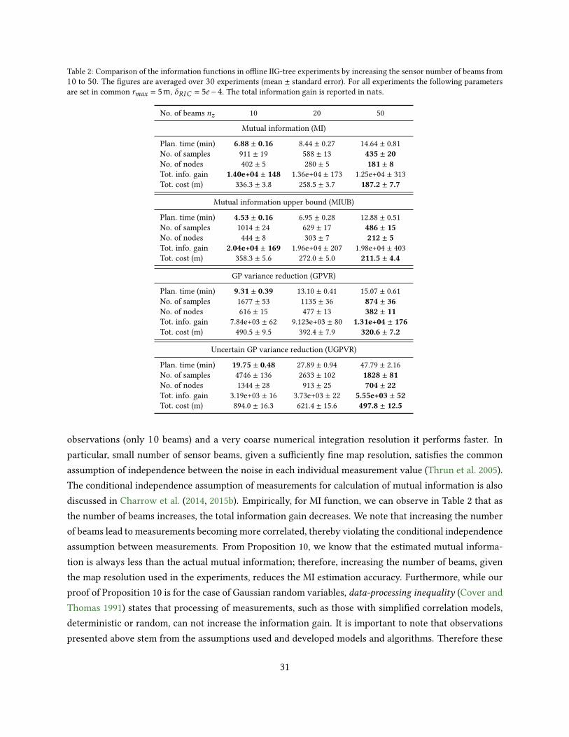
Table 2: Comparison of the information functions in oine IIG-tree experiments by increasing the sensor number of beams from10 to 50. The gures are averaged over 30 experiments (mean ± standard error). For all experiments the following parametersare set in common rmax = 5m, δRIC = 5e − 4. The total information gain is reported in nats.

No. of beams nz 10 20 50

Mutual information (MI)

Plan. time (min) 6.88 ± 0.16 8.44 ± 0.27 14.64 ± 0.81No. of samples 911 ± 19 588 ± 13 435 ± 20No. of nodes 402 ± 5 280 ± 5 181 ± 8Tot. info. gain 1.40e+04 ± 148 1.36e+04 ± 173 1.25e+04 ± 313Tot. cost (m) 336.3 ± 3.8 258.5 ± 3.7 187.2 ± 7.7

Mutual information upper bound (MIUB)


GP variance reduction (GPVR)


Uncertain GP variance reduction (UGPVR)


observations (only 10 beams) and a very coarse numerical integration resolution it performs faster. Inparticular, small number of sensor beams, given a suciently ne map resolution, satises the commonassumption of independence between the noise in each individual measurement value (Thrun et al. 2005).The conditional independence assumption of measurements for calculation of mutual information is alsodiscussed in Charrow et al. (2014, 2015b). Empirically, for MI function, we can observe in Table 2 that asthe number of beams increases, the total information gain decreases. We note that increasing the numberof beams lead to measurements becoming more correlated, thereby violating the conditional independenceassumption between measurements. From Proposition 10, we know that the estimated mutual informa-tion is always less than the actual mutual information; therefore, increasing the number of beams, giventhe map resolution used in the experiments, reduces the MI estimation accuracy. Furthermore, while ourproof of Proposition 10 is for the case of Gaussian random variables, data-processing inequality (Cover andThomas 1991) states that processing of measurements, such as those with simplied correlation models,deterministic or random, can not increase the information gain. It is important to note that observationspresented above stem from the assumptions used and developed models and algorithms. Therefore these

31

Table 3: Comparison of the information functions in oine IIG-tree experiments by increasing the sensor range, rmax , from 5mto 20m (averaged over 30 experiments, mean ± standard error). For all experiments the following parameters are set in commonnz = 10; δRIC = 5e − 4. The total information gain is reported in nats.

Range rmax (m) 5 10 20

Mutual information (MI)


Mutual information upper bound (MIUB)


GP variance reduction (GPVR)


Uncertain GP variance reduction (UGPVR)


results should not be interpreted to indicate that in general using a sparse set of measurements the infor-mation gain calculation accuracy increases.

For all the compared algorithms, as the number of beams increases, i.e. taking more observations,the computations take longer, and the number of samples/nodes reduces. However, MI has the fastestconvergence speed with, approximately, half of the number of samples taken by GPVR. Incorporatingthe pose uncertainty in UGPVR leads to a slower convergence. This can be explained as a result of thereduction in the information content of each set of observations by adding uncertainty to the informationgain calculation. Another interpretation is that the UGPVR algorithm is, relatively speaking, less greedyor more conservative for information gathering. For GPVR-based information functions, increasing thenumber of sensor beams, leads to higher total information gain due to a larger training set D. MI incomparison with MIUB has more realistic information gain estimation which is reected in less total coston average. In other words, the upper bound of the estimated MI, most likely, overestimate the actualinformation gain (Lemma 1). The latter results also conrm the advantage of maximizing the mutualinformation rather than minimizing the entropy which is discussed in Krause et al. (2008).

32

0 5 10 15 200

5

10

15

20

0 5 10 15 200

5

10

15

20

0 5 10 15 200

5

10

15

20

Figure 3: An example of results from running the IIG-tree algorithm in the Cave map. From top left, the plots show the IIG-treegraph for MI, MIUB, GPVR, and UGPVR MI information functions. The selected paths computed using Algorithm 7 are alsoshown where the most informative path is shown using a darker color. MI and UGPVR show similar behaviors despite dierentquantitative outcomes. The last two plots in the bottom row, from left, show the convergence graph of the penalized relativeinformation contribution IRIC and the evolution of the cumulative information gain for all information functions, respectively.The sensor range and the number of beams are set to 5m and 10, respectively.

Figure 3 illustrates examples of IIG-tree results using dierent information functions in the Cave map.The sensor range and the number of beams are set to 5m and 10, respectively. The extracted paths are alsoshown and the most informative path is separated using a darker color. The convergence of IRIC for allinformation is shown in bottom middle plot, and the bottom right plot shows the cumulative informationgain demonstrating its diminishing return over time (as the number of samples grows). The higher valueof IRIC can be correlated with a denser IIG graph. Also, the MIUB essentially minimizes the entropywhich tends to explore the boundary of the space, unlike MI that takes into account the perception eldof the sensor. This behavior is also observed and discussed in Krause et al. (2008, Figure 4). The GPVRand UGPVR curves have similar trends; however, due to the incorporated pose uncertainty the amount ofinformation gain is remarkably lower which explains the longer tail of information gain evolution beforethe convergence of the algorithm and the higher relative information contribution from each node. In

33

other words, farther nodes have higher pose uncertainties. Therefore the discrimination between fartherand nearer nodes from relative information contribution is less than the case where the pose uncertaintyis ignored.

In the second experiment, the number of beams is kept xed at nz = 10, but the sensor range is in-creased from 5m to 20m. The results shown in Table 3 are consistent with the previous test. The variationsare smaller as the growth in the size of the observation set (training set for GPVR-based functions), due toincreased range, is much smaller, mostly as a result of the geometry of the environment. Note that the rstcolumn of Table 3 and rst column of Table 2 are for two dierent runs with same parameters. The dif-ferences in planning time are due to the fact that the experiments were carried out in a high-performancecomputing facility where the reported time is aected by other users activities. Furthermore, the dierencebetween rmax = 10 and rmax = 20 cases is marginal which shows increasing the sensor range more than10m does not improve the information gathering process in this particular environment.

Finally, a practical conclusion can be that increasing the sensor range and the number of beams (obser-vations) increases the computational time but does not necessarily make the corresponding informationfunction superior. As long as the approximation can capture the essence of information gain estimationconsistently, the search algorithm performs well. Clearly the shape of the environment aects the result,e.g. the maximum and minimum perception eld at dierent areas of the map. For the experiments in thefollowing section, we select nz = 10 and rmax = 5m which lead to the fastest computational time withreasonable total information gain and cost values.

9.3 Robotic exploration in unknown environments

In this section, we examine use of the proposed algorithms for autonomous robotic exploration in anunknown environment (Figure 4). This requires solving the SLAM problem for localization possibly usingobservations to features in the environment. It is also necessary to build a dense map representation thatshows occupied and unoccupied regions for planning and navigation. We solve the localization problemusing Pose SLAM, the occupancy mapping using I-GPOM, and the planning using IIG-tree with dierentinformation functions. The I-GPOM models the occupancy map of the environment as GPs which can beused by IIG to implement the proposed GPVR-based information functions.

We also compare our results with Active Pose SLAM (APS) (Valencia et al. 2012) which is an informa-tion gain-based technique that considers explicit loop-closures by searching through nearby poses in thepose graph. As APS uses an Occupancy Grid Map (OGM) (Moravec and Elfes 1985; Elfes 1987) for map-ping and frontiers (Yamauchi 1997) as exploration target candidates, we generate the equivalent I-GPOMusing all poses and observations at the end of an experiment in order to compare mapping performance.Pose SLAM parameters were set and xed regardless of the exploration method. The localization RootMean Square Error (RMSE) was computed at the end of each experiment by the dierence in the robotestimated and ground truth poses. The occupancy maps are compared using the Area Under the receiveroperating characteristic Curve (AUC) as AUC is known to be more suitable for domains with skewed class

34

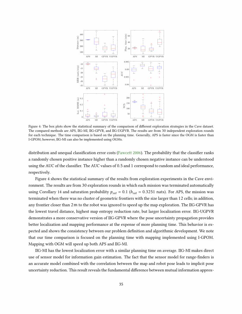
Figure 4: The box plots show the statistical summary of the comparison of dierent exploration strategies in the Cave dataset.The compared methods are APS, IIG-MI, IIG-GPVR, and IIG-UGPVR. The results are from 30 independent exploration roundsfor each technique. The time comparison is based on the planning time. Generally, APS is faster since the OGM is faster thanI-GPOM; however, IIG-MI can also be implemented using OGMs.

distribution and unequal classication error costs (Fawcett 2006). The probability that the classier ranksa randomly chosen positive instance higher than a randomly chosen negative instance can be understoodusing the AUC of the classier. The AUC values of 0.5 and 1 correspond to random and ideal performance,respectively.

Figure 4 shows the statistical summary of the results from exploration experiments in the Cave envi-ronment. The results are from 30 exploration rounds in which each mission was terminated automaticallyusing Corollary 14 and saturation probability psat = 0.1 (hsat = 0.3251 nats). For APS, the mission wasterminated when there was no cluster of geometric frontiers with the size larger than 12 cells; in addition,any frontier closer than 2m to the robot was ignored to speed up the map exploration. The IIG-GPVR hasthe lowest travel distance, highest map entropy reduction rate, but larger localization error. IIG-UGPVRdemonstrates a more conservative version of IIG-GPVR where the pose uncertainty propagation providesbetter localization and mapping performance at the expense of more planning time. This behavior is ex-pected and shows the consistency between our problem denition and algorithmic development. We notethat our time comparison is focused on the planning time with mapping implemented using I-GPOM.Mapping with OGM will speed up both APS and IIG-MI.

IIG-MI has the lowest localization error with a similar planning time on average. IIG-MI makes directuse of sensor model for information gain estimation. The fact that the sensor model for range-nders isan accurate model combined with the correlation between the map and robot pose leads to implicit poseuncertainty reduction. This result reveals the fundamental dierence between mutual information approx-

35

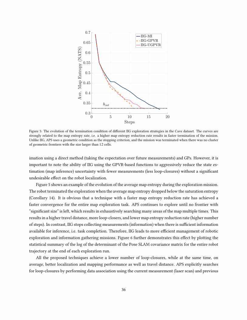
Figure 5: The evolution of the termination condition of dierent IIG exploration strategies in the Cave dataset. The curves arestrongly related to the map entropy rate, i.e. a higher map entropy reduction rate results in faster termination of the mission.Unlike IIG, APS uses a geometric condition as the stopping criterion, and the mission was terminated when there was no clusterof geometric frontiers with the size larger than 12 cells.

imation using a direct method (taking the expectation over future measurements) and GPs. However, it isimportant to note the ability of IIG using the GPVR-based functions to aggressively reduce the state es-timation (map inference) uncertainty with fewer measurements (less loop-closures) without a signicantundesirable eect on the robot localization.

Figure 5 shows an example of the evolution of the average map entropy during the exploration mission.The robot terminated the exploration when the average map entropy dropped below the saturation entropy(Corollary 14). It is obvious that a technique with a faster map entropy reduction rate has achieved afaster convergence for the entire map exploration task. APS continues to explore until no frontier with“signicant size” is left, which results in exhaustively searching many areas of the map multiple times. Thisresults in a higher travel distance, more loop-closers, and lower map entropy reduction rate (higher numberof steps). In contrast, IIG stops collecting measurements (information) when there is sucient informationavailable for inference, i.e. task completion. Therefore, IIG leads to more ecient management of roboticexploration and information gathering missions. Figure 6 further demonstrates this eect by plotting thestatistical summary of the log of the determinant of the Pose SLAM covariance matrix for the entire robottrajectory at the end of each exploration run.

All the proposed techniques achieve a lower number of loop-closures, while at the same time, onaverage, better localization and mapping performance as well as travel distance. APS explicitly searchesfor loop-closures by performing data association using the current measurement (laser scan) and previous

36

Figure 6: The statistical summary of the log of the determinant of the Pose SLAM covariance matrix at the end of each explorationrun in the Cave dataset. The compared methods are, from left, APS, IIG-MI, IIG-GPVR, and IIG-UGPVR. IIG algorithms canterminate the information gathering process when there is sucient information available for inference according to the requestedsaturation entropy (termination condition). Such an ability is not available in the APS framework since the robot has to completethe map based on its geometrical shape.

scans with nearby poses available in the pose graph. This is a particularly expensive process and oftenlimits the search area to small regions, especially, when the SLAM graph becomes less sparse due to thelarge number of loop-closures. Lastly, we would like to emphasize that IIG-UGPVR is a fully integratedinformation-theoretic planner that takes full state estimate (the robot pose and map) uncertainty intoaccount, it oers an automatic termination condition for the entire mission, has an adjustable planninghorizon, δRIC , and treats future measurements as random by taking expectations over them. In constrast,APS simplies the information gain computation by resorting to a conditional independence assumptionbetween the robot pose and the map. The true strength of APS for achieving comparable outcomes isthrough shifting the computational load towards the data association for predicting informative loop-closures along a planned trajectory. Therefore, the work presented in this paper is an alternative that isfundamentally dierent. Furthermore, the termination condition proposed in this article is general andcan be easily incorporated into APS or other exploration techniques. For examples of qualitative resultsincluidng Pose SLAM, I-GPOM, and OGM plots see Ghaari Jadidi et al. (2016); Ghaari Jadidi (2017).

9.4 Lake monitoring experiment

In this experiment, we demonstrate the performance of IIGs in a lake monitoring scenario. The ASVcan localize using a GPS unit and a Doppler Velocity Log. The communication with the ground station

37

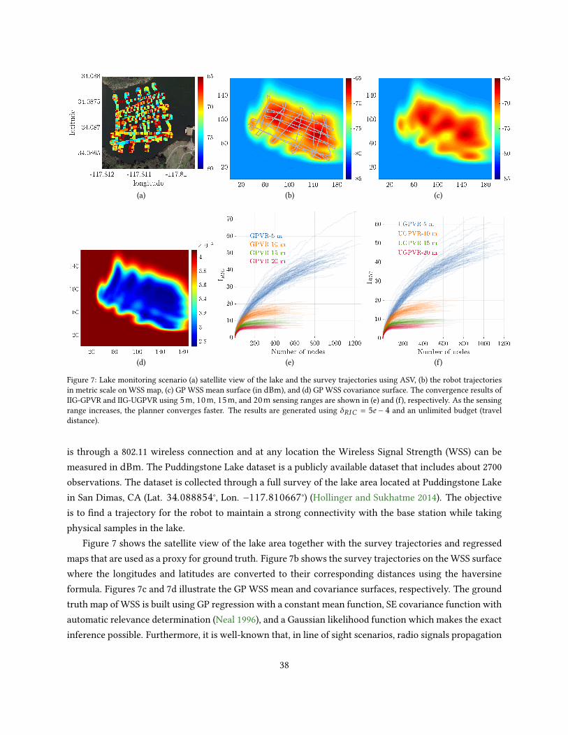
(a) (b) (c)

(d) (e) (f)

Figure 7: Lake monitoring scenario (a) satellite view of the lake and the survey trajectories using ASV, (b) the robot trajectoriesin metric scale on WSS map, (c) GP WSS mean surface (in dBm), and (d) GP WSS covariance surface. The convergence results ofIIG-GPVR and IIG-UGPVR using 5m, 10m, 15m, and 20m sensing ranges are shown in (e) and (f), respectively. As the sensingrange increases, the planner converges faster. The results are generated using δRIC = 5e − 4 and an unlimited budget (traveldistance).

is through a 802.11 wireless connection and at any location the Wireless Signal Strength (WSS) can bemeasured in dBm. The Puddingstone Lake dataset is a publicly available dataset that includes about 2700observations. The dataset is collected through a full survey of the lake area located at Puddingstone Lakein San Dimas, CA (Lat. 34.088854°, Lon. −117.810667°) (Hollinger and Sukhatme 2014). The objectiveis to nd a trajectory for the robot to maintain a strong connectivity with the base station while takingphysical samples in the lake.

Figure 7 shows the satellite view of the lake area together with the survey trajectories and regressedmaps that are used as a proxy for ground truth. Figure 7b shows the survey trajectories on the WSS surfacewhere the longitudes and latitudes are converted to their corresponding distances using the haversineformula. Figures 7c and 7d illustrate the GP WSS mean and covariance surfaces, respectively. The groundtruth map of WSS is built using GP regression with a constant mean function, SE covariance function withautomatic relevance determination (Neal 1996), and a Gaussian likelihood function which makes the exactinference possible. Furthermore, it is well-known that, in line of sight scenarios, radio signals propagation

38

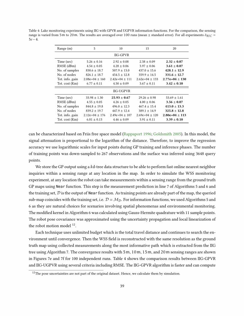
Table 4: Lake monitoring experiments using IIG with GPVR and UGPVR information functions. For the comparison, the sensingrange is varied from 5m to 20m. The results are averaged over 100 runs (mean ± standard error). For all experiments δRIC =5e − 4.

Range (m) 5 10 15 20

IIG-GPVR

Time (sec) 5.26 ± 0.16 2.92 ± 0.08 2.38 ± 0.09 2.32 ± 0.07RMSE (dBm) 4.54 ± 0.05 4.28 ± 0.06 3.97 ± 0.06 3.61 ± 0.07No. of samples 830.6 ± 18.7 507.9 ± 13.0 437.0 ± 15.6 428.1 ± 12.9No. of nodes 826.1 ± 18.7 454.5 ± 12.8 359.9 ± 14.5 331.6 ± 12.7Tot. info. gain 2.08e+04 ± 160 2.42e+04 ± 111 2.62e+04 ± 133 2.77e+04 ± 130Tot. cost (Km) 6.77 ± 0.11 4.50 ± 0.09 3.67 ± 0.11 3.42 ± 0.10

IIG-UGPVR

Time (sec) 33.98 ± 1.30 25.93 ± 0.67 29.26 ± 0.98 53.69 ± 1.61RMSE (dBm) 4.55 ± 0.05 4.26 ± 0.05 4.00 ± 0.06 3.56 ± 0.07No. of samples 844.8 ± 19.8 496.0 ± 12.3 467.4 ± 15.4 413.0 ± 13.3No. of nodes 839.2 ± 19.7 447.9 ± 12.4 389.1 ± 14.9 325.8 ± 12.8Tot. info. gain 2.12e+04 ± 176 2.49e+04 ± 107 2.69e+04 ± 120 2.80e+04 ± 113Tot. cost (Km) 6.81 ± 0.13 4.46 ± 0.09 3.91 ± 0.11 3.39 ± 0.10

can be characterized based on Friis free space model (Rappaport 1996; Goldsmith 2005). In this model, thesignal attenuation is proportional to the logarithm of the distance. Therefore, to improve the regressionaccuracy we use logarithmic scales for input points during GP training and inference phases. The numberof training points was down-sampled to 267 observations and the surface was inferred using 3648 querypoints.

We store the GP output using a kd-tree data structure to be able to perform fast online nearest neighborinquiries within a sensing range at any location in the map. In order to simulate the WSS monitoringexperiment, at any location the robot can take measurements within a sensing range from the ground truthGP maps using Near function. This step is the measurement prediction in line 7 of Algorithms 5 and 6 andthe training set,D is the output of Near function. As training points are already part of the map, the queriedsub-map coincides with the training set, i.e. D =MD. For information functions, we used Algorithms 5 and6 as they are natural choices for scenarios involving spatial phenomenas and environmental monitoring.The modied kernel in Algorithm 6 was calculated using Gauss-Hermite quadrature with 11 sample points.The robot pose covariance was approximated using the uncertainty propagation and local linearization ofthe robot motion model 12.

Each technique uses unlimited budget which is the total travel distance and continues to search the en-vironment until convergence. Then the WSS eld is reconstructed with the same resolution as the groundtruth map using collected measurements along the most informative path which is extracted from the IIGtree using Algorithm 7. The convergence results with 5m, 10m, 15m, and 20m sensing ranges are shownin Figures 7e and 7f for 100 independent runs. Table 4 shows the comparison results between IIG-GPVRand IIG-UGPVR using several criteria including RMSE. The IIG-GPVR algorithm is faster and can compute

12The pose uncertainties are not part of the original dataset. Hence, we calculate them by simulation.

39

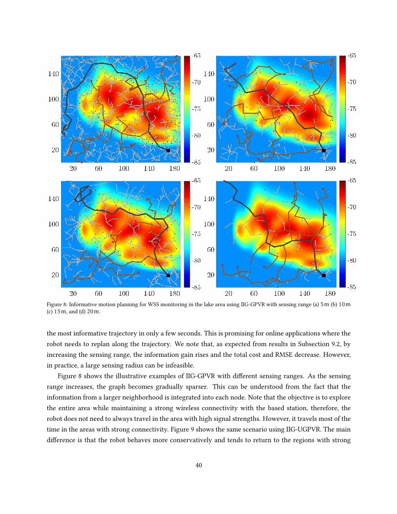
Figure 8: Informative motion planning for WSS monitoring in the lake area using IIG-GPVR with sensing range (a) 5m (b) 10m(c) 15m, and (d) 20m.

the most informative trajectory in only a few seconds. This is promising for online applications where therobot needs to replan along the trajectory. We note that, as expected from results in Subsection 9.2, byincreasing the sensing range, the information gain rises and the total cost and RMSE decrease. However,in practice, a large sensing radius can be infeasible.

Figure 8 shows the illustrative examples of IIG-GPVR with dierent sensing ranges. As the sensingrange increases, the graph becomes gradually sparser. This can be understood from the fact that theinformation from a larger neighborhood is integrated into each node. Note that the objective is to explorethe entire area while maintaining a strong wireless connectivity with the based station, therefore, therobot does not need to always travel in the area with high signal strengths. However, it travels most of thetime in the areas with strong connectivity. Figure 9 shows the same scenario using IIG-UGPVR. The maindierence is that the robot behaves more conservatively and tends to return to the regions with strong

40

Figure 9: Informative motion planning for WSS monitoring in the lake area using IIG-UGPVR with sensing range (a) 5m (b) 10m(c) 15m, and (d) 20m. By incorporating pose uncertainties in planning, the informative trajectories are those in which not onlythe wireless connectivity is strong, but the pose uncertainty along the trajectories is minimized.

connectivity. The growth in pose uncertainty by traveling farther, reduces the information gain of thoseareas. In both IIG-GPVR and IIG-UGPVR results, we can see that by increasing the sensing range the robottends to explore farther distances which is a natural behavior, in Figures 8d and 9d.

9.5 Limitations and observations

The proposed algorithms can provide an approximate solution to the robotic exploration problem in un-known environments as a basic navigation task as well as environmental monitoring tasks. Although IIGcan be implemented for online tasks, it has the limitations of its ancestors. Therefore, violating the mainassumptions, such as availability of free area near any point for graph expansion, can result in failure ofthe task. More conceptually, most of the present robotic navigation algorithms are not truly adaptive as

41

they commit to a decision once it is planned and replanning occurs only if the amount of computation ismanageable, and often not with a high frequency. So there will be a window of time the robot acts basedon the previously made decision. Although humans act in a similar fashion, we can make decisions morespontaneously (fully adaptive). This problem can be severe in environments that are highly dynamic asthe robot is not as responsive as it is required.

To our experience, using a coarse approximation, i.e. less number of beams than the actual range-ndersensor results in not only faster search in the workspace and reducing the computational time, but givingthe chance to more samples to be candidates as part of the potential most informative path. This is apromising feature that the algorithm works reasonably well without near exact estimation of informationquality. Moreover, uniform sampling produces reasonable results in the early stage, however as the graphgrows, this sampling strategy becomes less ecient. Biasing the sampling towards directions that are lessexplored may lead to a faster convergence.

10 Conclusion and future Work

In this work, we developed a sampling-based planning algorithm for incremental robotic information gath-ering. The proposed algorithm is based on RIG and oers an information-theoretic convergence criterionusing the notion of penalized relative information contribution. We formulated the problem as an infor-mation maximization problem subject to budget and state estimate constraints. The unique feature of thisapproach is that it can handle dense belief representations as well as the robot pose uncertainty. We pro-posed MI-based and GPVR-based information functions that can be used in both RIG and IIG frameworks.The proposed IIG-tree algorithm using a UGPVR information function considers pose uncertainties inplanning and provides an approximate solution for nding maximally informative paths under partiallyobservable state variables.

We proved an information-theoretic termination condition for the entire information gathering mis-sion based on the least upper bound of the average state variables entropy. The proposed algorithms candirectly be applied to environmental monitoring and robotic exploration tasks in unknown environments.The proposed algorithms have also potential applications in solving the sensor conguration selectionproblem that we did not fully investigate as it is beyond the scope of this work. Furthermore, the planninghorizon does not need to be set as a number of steps. Instead, the information-theoretic representation ofthe planning horizon used here brings more exibility for managing the convergence of the algorithm.

We would like to share some ideas that are natural extensions of this work. For the sake of clarity, weitemize them as follows.

(i) The algorithms in this article could be extended for multi-robot planning; exploiting the informationgain available through wireless communication channels to manage the coordination between robotswhile a feedback controller satised kinodynamic constraints.

(ii) We developed IIG-tree based on the RIG-tree algorithm. IIG could also be used to extend RIG-

42

roadmap and RIG-graph. RIG-graph is asymptotically optimal and can asymptotically explore allpossible budget-constraint trajectories, it produces a fully connected graph and is an interestingcase to study.

(iii) While we provide a procedural implementation of the proposed algorithms, and it suces for re-search and comparison purposes, we believe the integration of the algorithms in open source librariessuch as the Open Motion Planning Library (OMPL) (Sucan et al. 2012) has advantages for possibleapplications of this work.

(iv) The GPVR-based algorithms could be used for active learning to model the quantity of interest onlineusing GPs.

(v) IIG/RIG frameworks could be used for maximizing a multi-objective information function to performmultiple tasks concurrently. In a naïve approach, the objective function can be dened as the sumof information functions; however, if random variables from dierent information functions arecorrelated, e.g. through the robot pose, the total information gain calculation will not be accurate.Hence, developing a more systematic approach is an interesting avenue to follow.

(vi) A sparse covariance matrix could be constructed using the Sparse covariance function. Exploiting thesparse structure of the covariance matrix for large-scale problems could be an interesting extensionof this work for online implementations.

Appendices

A Proof of mutual information approximation inequality

In this Appendix, we provide the proof for Proposition 10. First, we present the required preliminaries andthen our proof by contradiction.

Lemma 3 (Hadamard’s Inequality). Let A = [a1 a2 · · · an] be an n × n matrix such that ai ∈ Rn for all

i ∈ 1 : n. Hadamard’s inequality asserts that

|A| ≤n∏i=1

‖ai‖ (27)

Corollary 15. Let S ∈ Rn×n be a positive denite matrix whose diagonal entries are s11, . . . , snn. From

Lemma 3, it follows that

|S| ≤n∏i=1

sii (28)

43

Proof. Since S is positive denite, using Cholesky factorization, we have S = LLT and |S| = |LLT | =|L||LT | = |L|2. For any diagonal elements of S, we have sii = lilTi = ‖li‖2 where li is the i-th column of L.Using the Hadamard’s inequality, it follows that

|S| = |L|2 ≤n∏i=1

‖li‖2 =n∏i=1

sii (29)

We now derive a few useful inequalities before the nal proof. Let X ∼N (µX ,ΣX) andX | Z ∼N (µX |Z ,ΣX |Z ) be the prior and posterior distribution of the n-dimensional random vector X,respectively. Let h(X) = 1

2 log((2πe)n|ΣX |) and h(X | Z) = 1

2 log((2πe)n|ΣX |Z |) be the dierential en-

tropy and conditional entropy, respectively; and I(X;Z) = h(X) − h(X | Z) the corresponding entropiesand mutual information by applying Proposition 9, where h(X) = 1

2 log((2πe)n∏n

i=1σXi ) and h(X | Z) =12 log((2πe)

n∏ni=1σXi |Z ). Using Corollary 15, the following inequalities are immediate:

h(X) ≤ h(X) (30)

h(X | Z) ≤ h(X | Z) (31)

I(X;Z) ≤ h(X)− h(X | Z) (32)

h(X)− h(X | Z) ≤ I(X;Z) (33)

h(X)− h(X | Z) ≤ h(X)− h(X | Z) (34)

and summing (32) and (33) leads to

I(X;Z) ≤ I(X;Z) + ξ(X;Z) (35)

where ξ(X;Z), h(X) + h(X | Z)− h(X)− h(X | Z) and ξ(X;Z) ≥ 0, with equality if and only ifX containsuncorrelated random variables, i.e. h(X) = h(X) and h(X | Z) = h(X | Z).

Proof of Proposition 10. Suppose I(X;Z) ≥ I(X;Z). By subtracting this inequality from (35) we have

I(X;Z)− I(X;Z)︸︷︷︸−a2

≤ I(X;Z)− I(X;Z)︸︷︷︸a2

+ξ(X;Z)

ξ(X;Z) ≥ −2a2

since ξ(X;Z) ≥ 0, a = 0 and I(X;Z) = I(X;Z) are the only possibilities. Now suppose I(X;Z) ≤ I(X;Z);

44

by summing this inequality and (35) we have

I(X;Z) + I(X;Z) ≤ I(X;Z) + I(X;Z) + ξ(X;Z)

ξ(X;Z) ≥ 0

which shows that information can only be lost and not gained.

References

Agha-mohammadi Aa, Chakravorty S and Amato NM (2014) FIRM: Sampling-based feedback motion-planning undermotion uncertainty and imperfect measurements. The Int. J. Robot. Res. 33(2): 268–304. 5

Astrom K (1965) Optimal control of Markov processes with incomplete state information. Journal of MathematicalAnalysis and Applications 10(1): 174–205. 5

Atanasov N, Le Ny J, Daniilidis K and Pappas GJ (2014) Information acquisition with sensing robots: Algorithms anderror bounds. In: Proc. IEEE Int. Conf. Robot Automat. IEEE, pp. 6447–6454. 5

Atanasov N, Le Ny J, Daniilidis K and Pappas GJ (2015) Decentralized active information acquisition: theory andapplication to multi-robot SLAM. In: Proc. IEEE Int. Conf. Robot Automat. IEEE, pp. 4775–4782. 5

Atanasov NA (2015) Active information acquisition with mobile robots. PhD Thesis, University of Pennsylvania. 5

Bertsekas DP (1995) Dynamic programming and optimal control, volume 1. Athena Scientic Belmont, MA. 5

Binney J, Krause A and Sukhatme GS (2013) Optimizing waypoints for monitoring spatiotemporal phenomena. TheInt. J. Robot. Res. 32(8): 873–888. 3, 5, 18

Binney J and Sukhatme GS (2012) Branch and bound for informative path planning. In: Proc. IEEE Int. Conf. RobotAutomat. IEEE, pp. 2147–2154. 3, 5, 12

Bry A and Roy N (2011) Rapidly-exploring random belief trees for motion planning under uncertainty. In: Proc. IEEEInt. Conf. Robot Automat. IEEE, pp. 723–730. 5, 11

Charrow B (2015) Information-theoretic active perception for multi-robot teams. PhD Thesis, University of Pennsyl-vania. 6

Charrow B, Kahn G, Patil S, Liu S, Goldberg K, Abbeel P, Michael N and Kumar V (2015a) Information-theoreticplanning with trajectory optimization for dense 3D mapping. In: Robotics: Science and Systems. 6

Charrow B, Liu S, Kumar V and Michael N (2015b) Information-theoretic mapping using Cauchy-Schwarz quadraticmutual information. In: Proc. IEEE Int. Conf. Robot Automat. IEEE, pp. 4791–4798. 6, 31

Charrow B, Michael N and Kumar V (2014) Cooperative multi-robot estimation and control for radio source local-ization. The Int. J. Robot. Res. 33(4): 569–580. 31

Cover TM and Thomas JA (1991) Elements of information theory. John Wiley & Sons. 7, 8, 31

45

Davis PJ and Rabinowitz P (1984) Methods of numerical integration. Academic Press. 23

Dhariwal A, Sukhatme GS and Requicha AA (2004) Bacterium-inspired robots for environmental monitoring. In:Proc. IEEE Int. Conf. Robot Automat., volume 2. IEEE, pp. 1436–1443. 3

Dunbabin M and Marques L (2012) Robots for environmental monitoring: Signicant advancements and applications.IEEE Robotics & Automation Magazine 19(1): 24–39. 3

Elfes A (1987) Sonar-based real-world mapping and navigation. Robotics and Automation, IEEE Journal of 3(3): 249–265. 34

Fawcett T (2006) An introduction to ROC analysis. Pattern recognition letters 27(8): 861–874. 35

Ghaari Jadidi M (2017) Gaussian Processes for Information-theoretic Robotic Mapping and Exploration. PhD Thesis.23, 37

Ghaari Jadidi M, Valls Miro J and Dissanayake G (2015) Mutual information-based exploration on continuous oc-cupancy maps. In: Proc. IEEE/RSJ Int. Conf. Intell. Robots Syst. pp. 6086–6092. 17

Ghaari Jadidi M, Valls Miro J and Dissanayake G (2016) Gaussian process autonomous mapping and explorationfor range sensing mobile robots. arXiv preprint arXiv:1605.00335 . 17, 22, 28, 37

Ghaari Jadidi M, Valls Miro J and Dissanayake G (2017) Warped Gaussian processes occupancy mapping withuncertain inputs. IEEE Robotics and Automation Letters 2(2): 680–687. 17, 23

Ghaari Jadidi M, Valls Miro J, Valencia R and Andrade-Cetto J (2014) Exploration on continuous Gaussian processfrontier maps. In: Proc. IEEE Int. Conf. Robot Automat. pp. 6077–6082. 10, 28

Goldsmith A (2005) Wireless communications. Cambridge university press. 39

Guestrin C, Krause A and Singh AP (2005) Near-optimal sensor placements in Gaussian processes. In: Proceedingsof the 22nd international conference on Machine learning. ACM, pp. 265–272. 18

Hollinger GA (2015) Long-horizon robotic search and classication using sampling-based motion planning. In:Robotics: Science and Systems. 6

Hollinger GA and Sukhatme GS (2013) Sampling-based motion planning for robotic information gathering. In:Robotics: Science and Systems. 3, 5

Hollinger GA and Sukhatme GS (2014) Sampling-based robotic information gathering algorithms. The Int. J. Robot.Res. 33(9): 1271–1287. 3, 5, 10, 11, 12, 28, 38

Horsch T, Schwarz F and Tolle H (1994) Motion planning with many degrees of freedom-random reections at c-spaceobstacles. In: Proc. IEEE Int. Conf. Robot Automat. IEEE, pp. 3318–3323. 5

Howard A and Roy N (2003) The robotics data set repository (Radish). URL http://radish.sourceforge.net. 30

Huynh VA and Roy N (2009) icLQG: combining local and global optimization for control in information space. In:Proc. IEEE Int. Conf. Robot Automat. IEEE, pp. 2851–2858. 5

46

http://radish.sourceforge.net

Ila V, Porta J and Andrade-Cetto J (2010) Information-based compact Pose SLAM. IEEE Trans. Robot. 26(1): 78–93. 28

Indelman V, Carlone L and Dellaert F (2015) Planning in the continuous domain: A generalized belief space approachfor autonomous navigation in unknown environments. The Int. J. Robot. Res. 34(7): 849–882. 5

Kaelbling LP, Littman ML and Cassandra AR (1998) Planning and acting in partially observable stochastic domains.Articial intelligence 101(1): 99–134. 5

Karaman S and Frazzoli E (2011) Sampling-based algorithms for optimal motion planning. The Int. J. Robot. Res. 30(7):846–894. 5, 11, 12

Kavraki LE, Švestka P, Latombe JC and Overmars MH (1996) Probabilistic roadmaps for path planning in high-dimensional conguration spaces. Robotics and Automation, IEEE Transactions on 12(4): 566–580. 5

Kim A and Eustice RM (2015) Active visual slam for robotic area coverage: Theory and experiment. The Int. J. Robot.Res. 34(4-5): 457–475. 3

Kim S and Kim J (2015) GPmap: A unied framework for robotic mapping based on sparse Gaussian processes. In:Field and Service Robotics. Springer, pp. 319–332. 10

Krause A, Singh A and Guestrin C (2008) Near-optimal sensor placements in Gaussian processes: Theory, ecientalgorithms and empirical studies. The Journal of Machine Learning Research 9: 235–284. 8, 18, 32, 33

Kurniawati H, Du Y, Hsu D and Lee WS (2011) Motion planning under uncertainty for robotic tasks with long timehorizons. The Int. J. Robot. Res. 30(3): 308–323. 5

Kurniawati H, Hsu D and Lee WS (2008) Sarsop: Ecient point-based POMDP planning by approximating optimallyreachable belief spaces. In: Robotics: Science and Systems. 5

Lan X and Schwager M (2013) Planning periodic persistent monitoring trajectories for sensing robots in Gaussianrandom elds. In: Proc. IEEE Int. Conf. Robot Automat. IEEE, pp. 2415–2420. 3, 5

Latombe JC (1991) Robot motion planning, volume 124. Springer US. 5

LaValle SM (2006) Planning algorithms. Cambridge university press. 5

LaValle SM and Kuner JJ (2001) Randomized kinodynamic planning. The Int. J. Robot. Res. 20(5): 378–400. 5

Le Ny J and Pappas GJ (2009) On trajectory optimization for active sensing in Gaussian process models. In: Proc.IEEE Conf. Decision and Control. IEEE, pp. 6286–6292. 5

Leung C, Huang S and Dissanayake G (2006a) Active SLAM using model predictive control and attractor basedexploration. In: Proc. IEEE/RSJ Int. Conf. Intell. Robots Syst. IEEE, pp. 5026–5031. 5

Leung C, Huang S, Kwok N and Dissanayake G (2006b) Planning under uncertainty using model predictive controlfor information gathering. Robot. Auton. Syst. 54(11): 898–910. 5

Levine DS (2010) Information-rich path planning under general constraints using rapidly-exploring random trees. Mas-ter’s Thesis, Massachusetts Institute of Technology. 5, 26

47

Marchant R and Ramos F (2012) Bayesian optimisation for intelligent environmental monitoring. In: Proc. IEEE/RSJInt. Conf. Intell. Robots Syst. IEEE, pp. 2242–2249. 3

Melkumyan A and Ramos F (2009) A sparse covariance function for exact Gaussian process inference in large datasets.In: IJCAI, volume 9. pp. 1936–1942. 22

Moravec HP and Elfes A (1985) High resolution maps from wide angle sonar. In: Proc. IEEE Int. Conf. Robot Automat.,volume 2. IEEE, pp. 116–121. 34

Neal RM (1996) Bayesian learning for neural networks, volume 118. Springer New York. 38

Platt Jr R, Tedrake R, Kaelbling L and Lozano-Perez T (2010) Belief space planning assuming maximum likelihoodobservations. In: Robotics: Science and Systems. 5, 6

Prentice S and Roy N (2009) The belief roadmap: Ecient planning in belief space by factoring the covariance. TheInt. J. Robot. Res. 28(11-12): 1448–1465. 5

Press WH, Teukolsky SA, Vetterling WT and Flannery BP (1996) Numerical recipes in C, volume 2. Cambridgeuniversity press Cambridge. 23

Pukelsheim F (2006) Optimal design of experiments. Society for Industrial and Applied Mathematics. 20

Rappaport TS (1996) Wireless communications: principles and practice, volume 2. Prentice Hall PTR New Jersey. 39

Rasmussen C and Williams C (2006) Gaussian processes for machine learning, volume 1. MIT press. 9

Singh A, Krause A, Guestrin C and Kaiser WJ (2009) Ecient informative sensing using multiple robots. Journal ofArticial Intelligence Research : 707–755. 3, 5, 12

Singh A, Ramos F, Whyte HD and Kaiser WJ (2010) Modeling and decision making in spatio-temporal processes forenvironmental surveillance. In: Proc. IEEE Int. Conf. Robot Automat. IEEE, pp. 5490–5497. 3

Smallwood RD and Sondik EJ (1973) The optimal control of partially observable Markov processes over a nitehorizon. Operations Research 21(5): 1071–1088. 5

Stein M (1999) Interpolation of spatial data: some theory for kriging. Springer Verlag. 10

Ström DP, Nenci F and Stachniss C (2015) Predictive exploration considering previously mapped environments. In:Proc. IEEE Int. Conf. Robot Automat. IEEE, pp. 2761–2766. 3, 6

Sucan IA, Moll M and Kavraki LE (2012) The open motion planning library. IEEE Robotics & Automation Magazine19(4): 72–82. 43

Thrun S, Burgard W and Fox D (2005) Probabilistic robotics, volume 1. MIT press. 17, 31

Tresp V (2000) A Bayesian committee machine. Neural Computation 12(11): 2719–2741. 22

Valencia R, Morta M, Andrade-Cetto J and Porta JM (2013) Planning reliable paths with Pose SLAM. IEEE Trans.Robot. 29(4): 1050–1059. 5

48

Valencia R, Valls Miro J, Dissanayake G and Andrade-Cetto J (2012) Active Pose SLAM. In: Proc. IEEE/RSJ Int. Conf.Intell. Robots Syst. pp. 1885–1891. 34

Van Den Berg J, Abbeel P and Goldberg K (2011) LQG-MP: Optimized path planning for robots with motion uncer-tainty and imperfect state information. The Int. J. Robot. Res. 30(7): 895–913. 5

Von Mises R (1964) Mathematical theory of probability and statistics. Academic Press. 21

Yamauchi B (1997) A frontier-based approach for autonomous exploration. In: Int. Sym. Comput. Intell. Robot. Au-tomat. pp. 146–151. 3, 6, 34

Yu J, Karaman S and Rus D (2015) Persistent monitoring of events with stochastic arrivals at multiple stations. IEEETrans. Robot. 31(3): 521–535. 3

49

sampling-based incremental information gathering …sampling-based incremental information gathering...

Documents