sampling approaches for road vehicle fuel consumption

Sampling approaches for road vehicle fuel consumption monitoring

M.A. Ktistakis, J. Pavlovic, G. Fontaras 2021

EUR 30420 EN

This publication is a Science for Policy report by the Joint Research Centre (JRC), the European Commission’s

science and knowledge service. It aims to provide evidence-based scientific support to the European policymaking

process. The scientific output expressed does not imply a policy position of the European Commission. Neither

the European Commission nor any person acting on behalf of the Commission is responsible for the use that

might be made of this publication. For information on the methodology and quality underlying the data used in

this publication for which the source is neither Eurostat nor other Commission services, users should contact the

referenced source. The designations employed and the presentation of material on the maps do not imply the

expression of any opinion whatsoever on the part of the European Union concerning the legal status of any

country, territory, city or area or of its authorities, or concerning the delimitation of its frontiers or boundaries.

Contact information

Name: Georgios Fontaras

Address: European Commission, Joint Research Centre (JRC), Via E. Fermi, 2749, 21027 Ispra VA, Italy

Email: [email protected]

Tel.: +39 033278-6425

EU Science Hub

https://ec.europa.eu/jrc

JRC122063

EUR 30420 EN

PDF ISBN 978-92-76-23986-4 ISSN 1831-9424 doi:10.2760/39369

Luxembourg: Publications Office of the European Union, 2021

© European Union, 2021

The reuse policy of the European Commission is implemented by the Commission Decision 2011/833/EU of 12

December 2011 on the reuse of Commission documents (OJ L 330, 14.12.2011, p. 39). Except otherwise noted,

the reuse of this document is authorised under the Creative Commons Attribution 4.0 International (CC BY 4.0)

licence (https://creativecommons.org/licenses/by/4.0/). This means that reuse is allowed provided appropriate

credit is given and any changes are indicated. For any use or reproduction of photos or other material that is not

owned by the EU, permission must be sought directly from the copyright holders.

All content © European Union, 2021, except: front cover page, Sergio Souza, “Aerial view of cars on road during

daytime", 2021. Source: Fotolia.com

How to cite this report: Ktistakis M.A., Pavlovic J., Fontaras G., Sampling approaches for road vehicle fuel

consumption monitoring, EUR 30420 EN, Publications Office of the European Union, Luxembourg, 2021, ISBN

978-92-76-23986-4, doi:10.2760/39369, JRC122063.

https://creativecommons.org/licenses/by/4.0/

i

Contents

Abstract ............................................................................................................... 1

Acknowledgements ................................................................................................ 2

Executive summary ............................................................................................... 3

1 Introduction ...................................................................................................... 6

1.1 Background................................................................................................. 6

1.2 Objectives .................................................................................................. 7

1.3 Structure of the report ................................................................................. 7

2 Methodology ..................................................................................................... 8

2.1 Statistical background .................................................................................. 8

2.1.1 Terminology and basic concepts ............................................................ 8

2.1.2 Designing a sampling scheme ................................................................ 9

2.2 Sampling methods ..................................................................................... 10

2.2.1 Simple random sampling .................................................................... 11

2.2.2 Stratified sampling ............................................................................. 12

2.2.3 Quota sampling ................................................................................. 15

2.3 Data Sources ............................................................................................ 16

2.3.1 Geco air ............................................................................................ 17

2.3.2 Spritmonitor.de ................................................................................. 18

2.3.3 Travelcard ........................................................................................ 18

2.3.4 European Environment Agency ............................................................ 18

3 Data analysis .................................................................................................. 20

3.1 Dataset Representativeness ........................................................................ 20

3.2 Fuel consumption gap analysis .................................................................... 24

3.3 Validation of sampling methods ................................................................... 27

3.3.1 Simple random sampling .................................................................... 27

3.3.2 Stratified sampling ............................................................................. 32

Stratifying by Fuel Type ................................................................. 33

Stratifying by type-approval CO2 emissions ...................................... 35

Univariate stratification .................................................................. 37

Multivariate Stratification ............................................................... 39

Strata specific estimators ............................................................... 40

3.3.3 Impact of non-sampling errors ............................................................ 42

3.3.4 Practical considerations for the implementation of quota sampling ........... 43

4 Conclusions .................................................................................................... 44

References ......................................................................................................... 45

List of abbreviations and definitions ....................................................................... 47

ii

List of figures ...................................................................................................... 48

List of tables ....................................................................................................... 49

Annexes ............................................................................................................. 50

Annex 1. Allocations and statistics ..................................................................... 50

1

Abstract

EU Regulations introduced in 2019 for light- and heavy- duty vehicles contain provisions

requiring the European Commission to set up a mechanism to monitor the real-world

representativeness of the fuel consumption determined during the type-approval tests.

This study proposes a sampling based approach to collect these data. Two probability-

sampling methods (simple random sampling and stratified sampling) and one non-

probability sampling method (quota sampling) are discussed. We use data from three user-

based datasets (IFPEN, Travelcard and Spritmonitor) and the 2018 European Environment

Agency CO2 monitoring dataset. All three user-based datasets provide fairly good

representations of their respective countries’ sub-fleets and to a lesser extent the whole

fleet. The standard deviation of the fuel consumption gap was consistently found to be

approximately 20%. For a population of 15 million vehicles, using simple random sampling,

and the standard deviation of the fuel consumption set at 20%, a sample of fewer than

3000 vehicles is required for estimating the average gap with a confidence level of 99%

and sampling error less than 1%. Multivariate stratification with three stratification

variables (vehicle manufacturer, fuel type and engine rated power) was the optimal

combination, reducing the sample size by around 28% compared to simple random sample.

Requiring strata specific estimators resulted to an increase of the sample size, as the

number of stratification variables increased. Non-sampling errors, such as inaccuracy of

On-Board Fuel and/or energy Consumption Monitor (OBFCM) device measurements, are

expected to lead to an increase of the required sample size by at least 20%. Samples using

quota sampling were taken and had a sampling error less than 3.5%.

2

Acknowledgements

The authors gratefully acknowledge the European Commission's colleagues at the

Directorate-General for Climate Action (DG CLIMA) and the Joint Research Centre (JRC),

in particular Carlos Serra, Filip Francois, Nikolaus Steininger, Dimitrios Komnos and

Nikiforos Zacharof for their helpful and constructive comments and revision that

significantly contributed to improving the final version of this report. The authors would

like to thank Pierre Michel, Alexandre Chasse, Sol Selene Rodriguez and Gilles Corde from

the Institut Français du Pétrole Energies Nouvelles (IFP Energies Nouvelles) and express

their highest appreciation for the provision of the French (Geco air) real-world dataset.

Also, authors would like to acknowledge the valuable support of Travelcard B.V., and

Norbert Ligterink from the Netherlands Organisation for Applied Scientific Research (TNO)

for supplying the Netherlands (Travelcard) real-world data used for the validation and

improvement of the methods elaborated in this report.

Authors

Markos Alexandros Ktistakis, Joint Research Centre

Jelica Pavlovic, Joint Research Centre

Georgios Fontaras, Joint Research Centre

3

Executive summary

The average official CO2 emissions of new passenger cars registered in the European Union

(EU) were reported to have reduced from 170 g/km in 2001 to 119 g/km in 2017, based

on the New European Driving Cycle (NEDC) test procedure. However, the reduction trends

observed in the real-world did not follow at the same pace, an observation that is generally

known as CO2 emissions gap. This gap was reported to widen substantially, from about 8%

in 2001 to about 40% in 2017. The major reason for the gap was the unrepresentativeness

of the official CO2 certification procedure, based on the NEDC and the inherent variability

of fuel consumption when operating in real-world conditions.

The European Commission (EC), acknowledging the issue, introduced the Worldwide

harmonized Light vehicles Test Cycle and Procedure (WLTP) in the type-approval procedure

from September 2017. For the purpose of CO2 target compliance checking, the WLTP will

be used from 2021 on. This new certification procedure will decrease the gap but does not

fully eliminate it. For heavy-duty vehicles, the real-world performance is more unclear, as

the lack of historical certification values and real-world emission measures have yet

prevented an exact quantification of the gap.

Regulation (EU) 2019/631 for light duty vehicles (LDV) as well as Regulation (EU)

2019/1242 for heavy duty vehicles (HDV) contain similar provisions requiring the

Commission to set up a mechanism to monitor the real-world representativeness of the

CO2 emissions determined during the type-approval tests. To this end, the EC shall collect

real-world fuel consumption and total distance travelled data (previously stored on-board)

and shall aggregate them into anonymised datasets, including categorization per

manufacturer, before making them public. To that aim, technical requirements and

procedures need to be determined. For light-duty vehicles, Commission Implementing

Regulation (EU) 2021/392 requires manufacturers and Member States to collect this data

from 2022 onwards. The expectation is that this mechanism will generate data from a

statistically relevant sample of the entire fleet.

In this light, the present study aims at providing a comprehensive analysis of suitable

sampling methods, focusing on optimizing and testing the methods. Sample size

calculations must be performed a priori. To reach a high precision and determine the

minimum sample sizes needed, knowledge of the targeted vehicles is required. For this,

data from 3 user-based datasets (Geco Air, Travelcard and Spritmonitor) were used. These

datasets are based on volunteering and the data do not come from the OBFCM. Geco air

is a mobile app calculating the CO2 emissions based on the vehicle characteristics and GPS

measurements. Travelcard and Spritmonitor are based on self-reported data of fuelling

events. CO2 emissions data gathered by the European Environment Agency (EEA) for all

new passenger cars registered in the Member States in 2018 were also utilised. The fuel

consumption gap for the vehicles recorded by EEA is not available. For the purposes of this

report it was simulated using the information about fuel consumption gap of the other

three datasets.

The representativeness of the three datasets and the sub-fleets of their respective

countries was examined in respect to fuel type, type approval CO2 emissions, vehicle

manufacturer, engine rated power and engine displacement. It was found that all datasets

provide fairly good representations of their respective countries sub-fleets and to a lesser

extent the EU fleet.

The fuel consumption gap was analysed firstly as a stand-alone variable, then in relation

to the other variables used in this report (fuel type, transmission type, vehicle

manufacturer, type approval CO2 emissions, engine rated power, engine displacement and

total distance driven). The standard deviation of the fuel consumption gap in the three user

datasets was consistently found to be approximately 20%.

Two probability sampling methods (simple random sampling and stratified sampling) and

one non-probability sampling method (quota sampling) were chosen and discussed in this

report. In simple random sampling, the higher the variability of the fuel consumption gap,

the higher the required sample size. For a fleet of 15 million vehicles, if the standard

4

deviation of the fuel consumption gap of the whole fleet is 20% (as inferred by the data

retrieved from the three sources) a sample of fewer than 3,000 vehicles is required for

estimating the average fleet-wide average gap with a confidence level of 99% and sampling

error less than 1%. If the standard deviation of the fuel consumption gap is 40% (an

assumption that is not validated by the data received from the three sources)

approximately 10,500 vehicles would be required to achieve this precision.

Stratified sampling can further reduce the required sample size for determining precisely

the fleet-wide average gap and also provide sufficient representation of sub-populations of

interest. Three different kinds of allocation procedures were examined, of which Neyman

allocation produced the best results, but requires extensive a priori knowledge of the

population. Different stratification variables were used, first separately (univariate

stratification) and then combinations of them (multivariate stratification). It was found that

multivariate stratification with three stratification variables (vehicle manufacturer, type-

fuel type and engine rated power) was the optimal combination requiring the least sample

size - about 28% less than simple random sampling. Increasing the number of stratification

variables offered marginally better results while increasing the difficulty and complexity of

the process.

The probability sampling methods were validated by simulating a large number of samples

and calculating the population error. In all cases, when a margin of error of 1% and a

confidence level of 99% was required, the sampling error was found to be in average 0.0%,

with a standard deviation less or equal to 0.6% (Table ES1).

When precise estimators are demanded not only for the fuel consumption gap of the whole

fleet, but also per stratum, the required sample size increases. The required sample size

escalates when the number of stratification variables increases. To get precise estimators

for all strata when stratifying by vehicle manufacturer, type-fuel type and engine rated

power, a sample of approximately 18,000 vehicles is needed (compared to ~ 2000 vehicles

with precise estimator of the whole population average fuel consumption gap only).

To understand the impact of non-sampling errors and more specifically of the OBFCM

inaccuracies on the sample size, a “noise” was added to the type approval and the real

world fuel consumption of all vehicles. This led to 2.5% higher standard deviation of the

fuel consumption gap of EEA vehicles, which resulted in a 26% increase of sample size

when using simple random sampling.

For quota sampling, it is not possible to estimate the sampling error because of the absence

of randomness. However to get an indication of the method’s effectiveness a quota sample

(with respect to the vehicle manufacturer, fuel type and engine rated power) was extracted

from each dataset. The sampling error in all four datasets was found to be less than 3.5%

(Table ES1).

5

Table ES1 Statistics of the sampling error

Dataset

Geco air (France)

Spritmonitor.de (Germany)

Travelcard

(Netherlands)

EEA

(EU)

Method share

(%)

mean

(%)

sd

(%)

share

(%)

mean

(%)

sd

(%)

share

(%)

mean

(%)

sd

(%)

share

(%)

mean

(%)

sd

(%)

Simple

random sampling

96.1 0.0 0.4 26.3 0.0 0.4 8.2 0.0 0.4 0.019 0.0 0.4

Stratified sampling by

OEM 81.9 0.0 0.4 25.0 0.0 0.4 7.5 0.0 0.4 0.015 0.0 0.4

Stratified sampling by OEM & Fuel

type

78.7 0.0 0.5 24.8 0.0 0.5 7.3 0.0 0.4 0.015 0.0 0.4


type & Power

82.7 0.0 0.6 21.0 0.0 0.6 6.4 0.0 0.5 0.014 0.0 0.5


type & Power & TA CO2

94.5 0.0 0.5 18.7 0.0 0.6 5.9 0.0 0.5 0.014 0.0 0.5

Quota sampling

82.7 2.8 - 21.0 1.5 - 6.4 3.2 - 0.014 2.1 -

Note: In parenthesis the countries where the majority of vehicles come from; margin of error 1%; confidence level 99%; sd: standard deviation; TA: type-approval, OEM: manufacturer; Power: engine rated power; share: percentage of the population sampled; population sizes: [Geco air:127, Spritmonitor.de:7,218, Travelcard:26,964 and EEA:14,623,747]

Source: JRC, 2021.

6

1 Introduction

1.1 Background

The first set of carbon dioxide (CO2) emission standards for passenger cars was introduced

in the European Union (EU) in 2009, (Regulation (EC) No 443/2009) and revised in 2014,

(Regulation (EU) No 333/2014). The emission values used for assessing compliance against

the targets are the official type-approval CO2 emissions of the vehicles. Over the course of

the last 20 years, data collected from experimental testing and self-reporting provided

indications of an increasing divergence between real-world CO2 emissions and fuel

consumption values and those reported officially, based on the New European Driving Cycle

(NEDC). Although the average official CO2 emissions of new passenger cars in the EU

reduced from 170 g/km in 2001 to 119 g/km in 2017, rebounding to 122 g/km in 2019,

the reduction trends observed in the actual operation (real-world measures) did not follow

at the same pace, an observation that is generally known as CO2 emissions gap. Most of

these analyses of real-world trends relied on statistical evaluations of voluntarily self-

reported consumer or fleet operator fuel consumption data. The gap was reported to widen

substantially, from about 8% in 2001 to about 40% in 2017 (Tietge et al. 2019; Fontaras

et al. 2017). This growth of the gap undermined the climate change mitigation efforts of

the EU CO2 standards and resulted in higher-than-expected fuel cost for consumers as well

as foregone tax revenue for governments (Tietge et al. 2019).

The major reason for the gap, highlighted by many studies (Fontaras et al 2017; Ligterink

et al. 2016; Tietge et al. 2019) was the unrepresentativeness of the official CO2 certification

procedure, based on the phasing-out methodology (NEDC) and the inherent variability of

fuel consumption when operating in real-world conditions. It is clear that no single

experimental test, no matter how complex, can capture the vast variety of a vehicle’s real-

world operating conditions. However, the main trends regarding emissions reduction and

efficiency improvements observed over the certification test should be reflected also in

real-operation, if not to their entirety, at least to a very large extent. The European

Commission (EC), acknowledging the issue of the non-representativeness of the NEDC-

based certification test introduced the Worldwide harmonized Light vehicles Test Cycle and

Procedure (WLTC and WLTP, respectively) in the type-approval procedure from September

2017 (Regulation 2017/1151). From 2021 on, the WLTP is the only cycle used for light-

duty vehicle CO2 certification in the EU. This new certification procedure is expected to

decrease the gap by more than half, to an order of about 20% when compared with the

certification average CO2 value (Pavlovic et al. 2018; Tsiakmakis et al. 2016). Dornoff et

al. 2020 confirm these estimates, suggesting that WLTP closes the gap by 22% to 24%

compared to the NEDC.

For heavy-duty vehicles (HDVs), the real-world performance is more unclear, the lack of

historical certification values and real-world emission measures have prevented an exact

quantification of the gap.

Regulation (EU) 2019/631 for passenger cars and light commercial vehicles (LDVs) as well

as Regulation (EU) 2019/1242 for HDVs, set new CO2 emission targets for 2025 and 2030.

Both Regulations also contain similar provisions requiring the Commission to set up a

mechanism to monitor the real-world representativeness of the CO2 emissions determined

during the type-approval or certification tests and the progression of any eventual

difference between the two. Also, the EC shall ensure that the public is informed on the

evolution of the gap over time and use these data to prevent the gap between type-

approval and real-world emissions from growing.

To this end, the Commission will collect real-world fuel and/or energy consumption and

distance travelled data from vehicles using On-Board Fuel and/or energy Consumption

Monitoring (OBFCM) devices. For LDVs such devices have been introduced in the type-

approval legislation through Regulation (EU) 2018/1832 (the so-called “WLTP 2nd-act”),

amending Regulation 2017/1151. For HDVs the standardization of OBFCM devices and their

type-approval requirements have not been introduced in a Regulation as yet. The two main

parameters concerned subject to future monitoring are the accumulated (lifetime) values

7

of fuel consumed and total distance travelled. Both these parameters shall be determined

and stored on-board of the vehicle, while also being unrestrictedly accessible through the

on-board diagnostics port (OBD). The data shall be then collected and transferred from the

vehicles to the EC and subsequently integrated into anonymised and aggregated datasets,

including per manufacturer. The EC shall assess how the collected data can be used to

ensure the real-world representativeness of CO2 emissions values determined during the

type-approval or certification tests. To that aim technical requirements and procedures

need to be determined. The EC has launched studies on the matter, trying to identify which

solutions are technically feasible, cost-effective, and adequate to satisfy the requirements

set by the Regulation.

For light-duty vehicles, Commission Implementing Regulation (EU) 2021/392 requires

manufacturers and Member States (through the Periodic Technical Inspections) to collect

this data from 2022 onwards. This approach shall be reviewed by the Commission by 2023,

in particular regarding the number of vehicles equipped with direct data transfer devices

and the need for continued monitoring and reporting of real-world data by manufacturers.

For heavy-duty vehicles, the Commission is still in the process of studying various data

collection options.

A sampling-based approach could give an acceptable precision and level of information for

the quantification of the gap with a limited margin of error and a very high confidence

level, while involving a minimum of resources. A detailed statistical analysis for determining

the different sampling methods that could be implemented, could help establish

approaches that will supplement the missing information and help establish a robust

monitoring approach.

1.2 Objectives

The goal of this study is to provide a comprehensive analysis of sampling approaches that

could support the monitoring of the CO2 emission and fuel consumption gap of road vehicles

for the fleet of new vehicles introduced in the EU. This includes:

1. Optimization of sampling i.e. minimum sample size that is representative of the

whole fleet within the acceptable error limits;

2. A reliable method of sample selection;

3. Comparison between different approaches;

4. Validation of the methods using both real-world and simulated data.

1.3 Structure of the report

The report is structured as follows:

Chapter 1 is an introduction to the current situation and the technical and policy-making

issues regarding the monitoring of the fuel consumption gap.

Chapter 2 provides the statistical background; describes the sampling approaches and

respective sample sizes and characteristics; introduces the datasets used in the analysis

and the pre-analysis performed.

Chapter 3 examines the representativeness of the datasets; the relationships between the

fuel consumption gap and the rest of the variables. It includes a validation of the different

sampling approaches using the datasets and presents an application for the different test

cases.

Chapter 4 summarizes the main conclusions of this report.

8

2 Methodology

2.1 Statistical background

2.1.1 Terminology and basic concepts

The following terms are used:

► (Target) population: The entire group of vehicles that the study is intended to

research and to which generalizations from samples are to be made. A measure of

a characteristic of the population is a parameter.

► Sampling Unit: Any single vehicle belonging to the population. Every vehicle being

regarded as individual and indivisible.

► Sample: A set of vehicles drawn from the population. Arithmetical characteristics of

the sample are called sample statistics, these are used as estimates of population

parameters.

► Sampling Frame: All sampling units from which those to be included in the sample

are selected. The sampling frame is a subset of the population and a superset of

the sample (Figure 1). Ideally, the sampling frame should be the same as the

population, but often this is not feasible.

► Census: A complete enumeration of the population. The observations of all vehicles

in the population are collected.

Figure 1 Depiction of relations between population, sampling frame and sample

Source: JRC, 2021.

A census does not have sampling error because all the units are measured. Yet it is easier

to conduct a sample survey than a census. In practice conducting a census might not be

plausible due to cost or technical limitations. By sampling it is possible to get reliable

information at far less cost than a census. Additionally, it is less time consuming, enabling

the publication of estimates in a timely fashion, while the sampling error from a survey can

be quantified by using probability samples. In some cases, estimates based on a census

can be less accurate than those based on a representative sample, because the data

gathering procedure and instrument can be designed to be of higher quality.

Sampling methods can be of two types depending on whether the sample selection

procedure used a probability mechanism or not:

► In probability sampling each vehicle has a predetermined non-zero chance to be

included in the sample. In this way, there are no selection biases, and statistical

theory can be used to extract properties of the estimators (e.g. the convergence of

9

the sample mean to the population mean). This category includes simple random

sampling, stratification, systematic sampling and cluster sampling.

► In non-probability sampling, vehicles are selected based on non-random criteria,

and not every vehicle has a chance of being selected. This type of sampling is easier

and costs less, but does not provide valid statistical inferences about the whole

population. In most cases, the vehicles are chosen supposing they are

representative of the population. There is subjectivity, which prevents the

development of a theoretical framework for it. Because of targeted selection, bias

can easily be introduced, and the possibility of generalizing and arriving at robust

findings is reduced. This category includes convenience sampling, quota sampling

and judgmental sampling.

Errors arising during a sampling procedure can be classified into two broad categories:

sampling errors and non-sampling errors.

► Sampling error is a statistical error that happens because the sample selected does

not represent perfectly the population of interest. The sampling error appears

because of the variation between the population and the sample parameters. In

probability sampling, sampling error can be quantified (by the margin of error and

confidence level, see 2.2.1) and reduced by increasing the sample size. In non-

probability sampling it cannot be quantified.

► Non-sampling error is an umbrella term which consists of all the errors, other than

the sampling error. It results because of a number of reasons, i.e. error in

questionnaire design, in problem definition, approach, data preparation, coverage,

information provided by respondents, tabulation, collection, and analysis. Non-

sampling errors can be found in all sampling methods (even in census). A non-

sampling error can be either random or systematic. Random errors usually offset

each other and therefore, most often, are of little concern. Systematic errors, on

the other hand, affect the entire sample and therefore present a more significant

issue. Non-sampling errors include: selection bias, sampling frame error, population

miss-specification error, non-response error, processing error, respondent error,

instrument error, surrogate error and interviewer error.

By designing properly all the steps of a statistical procedure (2.1.2) most types of error

can be minimized or even eliminated. In this case of quantifying the fuel consumption gap,

of great interest for the EC is to quantify and minimize the instrument error (OBFCM

accuracy).

2.1.2 Designing a sampling scheme

For designing a proper sampling procedure, the following aspects should be made clear:

► The purpose of the study: define the main research question. In this report the

purpose is to estimate the divergence between the real-world and the official type-

approval fuel consumption values for the whole fleet of new passenger cars

registered in the EU, which is quantified as the fuel consumption gap:

𝐹𝐶𝑔𝑎𝑝 =𝐹𝐶𝑅𝑊 − 𝐹𝐶𝑇𝐴

𝐹𝐶𝑇𝐴

∗ 100% (1)

where 𝐹𝐶𝑔𝑎𝑝 is the fuel consumption gap, 𝐹𝐶𝑇𝐴 is the type-approval fuel consumption and

𝐹𝐶𝑅𝑊 the real-world fuel consumption.

► The statement of objectives: define the secondary objectives of this research. In

this report these include :

o Estimate and compare the fuel consumption gap for different subpopulations

defined by known variables (see Table 1).

o Examine the representativeness of the user datasets with respect to

variables of interest (fuel type, type approval CO2 emissions, vehicle

manufacturer, engine rated power and engine displacement).

10

o Find trends and relationships/correlations between the fuel consumption gap

and other variables (see Table 1).

► The target population: specify the population of interest. The EC is interested in

studying two different populations: the LDVs and the HDVs introduced in the EU

from 2021 onwards. In this report, data analysis was conducted for LDVs, but the

same methods can be applied for HDVs as well.

► Access to the population: deciding on a sampling frame and how good it is. The

sampling frame should ideally be the closest possible to the whole population. If

this is not feasible, the sampling frame should represent as close as possible the

population. All vehicles registered in the EU are documented (section 2.3.4),

however, it is not yet clear when the real-world fuel consumption will be available

(see section 1.1).

► Data gathering procedure/instrument: determining the data collection method and

the accuracy of the measurements. The OBFCM monitored quantities will be

available at the on-board diagnostic (OBD) port in both LDVs and HDVs. These

devices will collect the real-world consumption, while the type-approval fuel

consumption will continue to be monitored by the European Environment Agency

(EEA). For LDVs the required accuracy of the OBFCMs for the fuel consumption is

set to 5% compared to the fuel consumption reported during WLTP type-approval

tests. EC is currently working on requirements for the OBFCMs accuracy for LDVs

and HDVs both at the lab and on-road (Pavlovic et al. 2021).

► Cost/budget: determining the cost of collecting the data, transferring them from

the OBFCM devices to the EC and processing them. Considering the budget allocated

from the EU and how it will be divided and if the sampling cost is the same for all

vehicles across the EU countries. In this report, costs are not included in the

analysis; cost-effectiveness will be one of the key factors for deciding any final

solution and shaping its eventual implementation.

► Sample size: determining the appropriate sample size in advance. Finding the best

compromise between accuracy considerations and cost/availability of the data.

Observations cost money, time and effort. Increasing the sample size above a

certain level gives minimal gains in terms of accuracy or representativeness.

► Quantifying the quantity of interest: deciding on which measures of location or

variability are going to be estimated. If the gap is measured for the whole

population (census) then the population measures of location and spread will be

known and no estimations will be needed. In case a sampling approach is used, the

result is going to be sampling measures of location and variability. These are

estimators of the respective population ones. With probability samples, the

sampling error can be quantified and confidence intervals can be constructed. In

this report, mainly the mean value and the standard deviation are used.

► Previous studies: studying and using the related bibliography.

► Sampling Technique: A suitable sampling method can be found by taking into

account the previous factors as well as the advantages and disadvantages of the

various sampling techniques. In this report there is one continuous variable of

interest (the fuel consumption gap), as well as information and interest for several

other variables (e.g. fuel type and manufacturer). Two probability sampling

methods were examined: simple random sampling and stratified sampling.

Additionally, quota sampling was proposed, in case probability sampling is not

feasible.

2.2 Sampling methods

Simple random sampling, stratifying sampling and quota sampling were the sampling

methods investigated in this report. Simple random sampling and stratifying sampling are

probability sampling methods, formulas for calculating the accuracy of the fuel

consumption gap using the sample are available. Utilising these formulas the required

11

sample size for achieving the demanded accuracy can be calculated in advance. Quota

sampling is a non-probability method, hence the extent to which valid inferences for the

population can be made using the sample is limited, but the criteria for choosing the sample

are less strict.

2.2.1 Simple random sampling

Simple random sampling is the simplest of the probability sampling techniques. The

principle is that each vehicle has the same probability of being selected. For example, for

getting a sample of n vehicles from the population of N new vehicles registered in the EU,

every vehicle could be assigned a number in the range from 1 to N, random numbers would

be generated, and the first n numbers selected would be the sample. This unbiased random

selection of vehicles is required to allow that the sample would accurately represent the

population.

This type of sampling requires a complete sampling frame. Advantages are that it is free

of classification error, no advance knowledge of the population is obligatory, and it is

relatively easy to interpret data collected. If more information is available stratified

sampling can be used. Simple random sampling can provide a benchmark for the required

sample size.

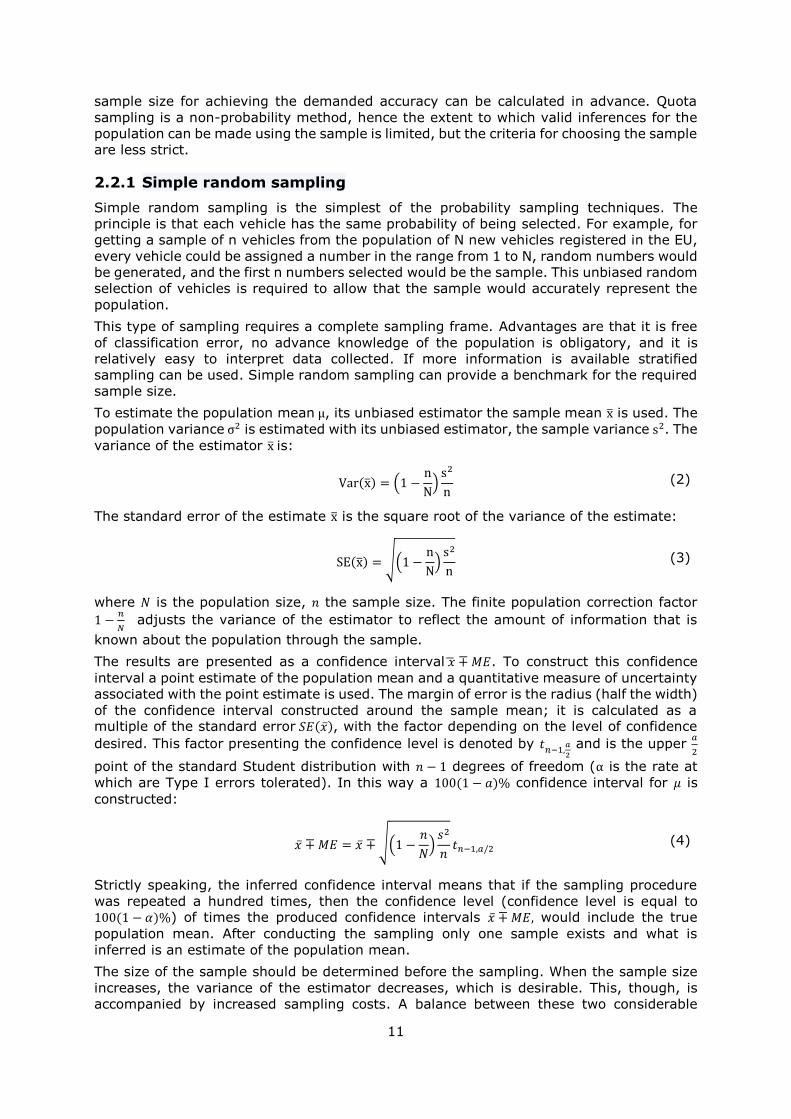
To estimate the population mean μ, its unbiased estimator the sample mean x̅ is used. The

population variance σ2 is estimated with its unbiased estimator, the sample variance s2. The

variance of the estimator x̅ is:

Var(x̅) = (1 −n

N)

s2

n (2)

The standard error of the estimate x̅ is the square root of the variance of the estimate:

SE(x̅) = √(1 −n

N)

s2

n (3)

where 𝑁 is the population size, 𝑛 the sample size. The finite population correction factor

1 −𝑛

𝑁 adjusts the variance of the estimator to reflect the amount of information that is

known about the population through the sample.

The results are presented as a confidence interval �̅� ∓ 𝑀𝐸. To construct this confidence

interval a point estimate of the population mean and a quantitative measure of uncertainty

associated with the point estimate is used. The margin of error is the radius (half the width)

of the confidence interval constructed around the sample mean; it is calculated as a multiple of the standard error 𝑆𝐸(�̅�), with the factor depending on the level of confidence

desired. This factor presenting the confidence level is denoted by 𝑡𝑛−1,

𝑎

2 and is the upper

𝑎

2

point of the standard Student distribution with 𝑛 − 1 degrees of freedom (α is the rate at

which are Type I errors tolerated). In this way a 100(1 − 𝑎)% confidence interval for 𝜇 is

constructed:

�̅� ∓ 𝑀𝐸 = �̅� ∓ √(1 −𝑛

𝑁)

𝑠2

𝑛𝑡𝑛−1,𝑎/2 (4)

Strictly speaking, the inferred confidence interval means that if the sampling procedure

was repeated a hundred times, then the confidence level (confidence level is equal to 100(1 − 𝛼)%) of times the produced confidence intervals �̅� ∓ 𝑀𝐸, would include the true

population mean. After conducting the sampling only one sample exists and what is

inferred is an estimate of the population mean.

The size of the sample should be determined before the sampling. When the sample size

increases, the variance of the estimator decreases, which is desirable. This, though, is

accompanied by increased sampling costs. A balance between these two considerable

12

aspects has to be considered. The sample size can be determined based on prescribed

values of the margin of error, i.e. by deciding on the desired multiple of the standard error.

An important constraint in determining the sample size is that information about the population variance 𝜎2 is a prerequisite. This could be dealt with by conducting a pilot

survey, i.e. collecting a preliminary sample, and use this survey’s sample variance as an

estimation of the population variance. It is also possible to estimate the population variance

from past data, experience, prior information etc.

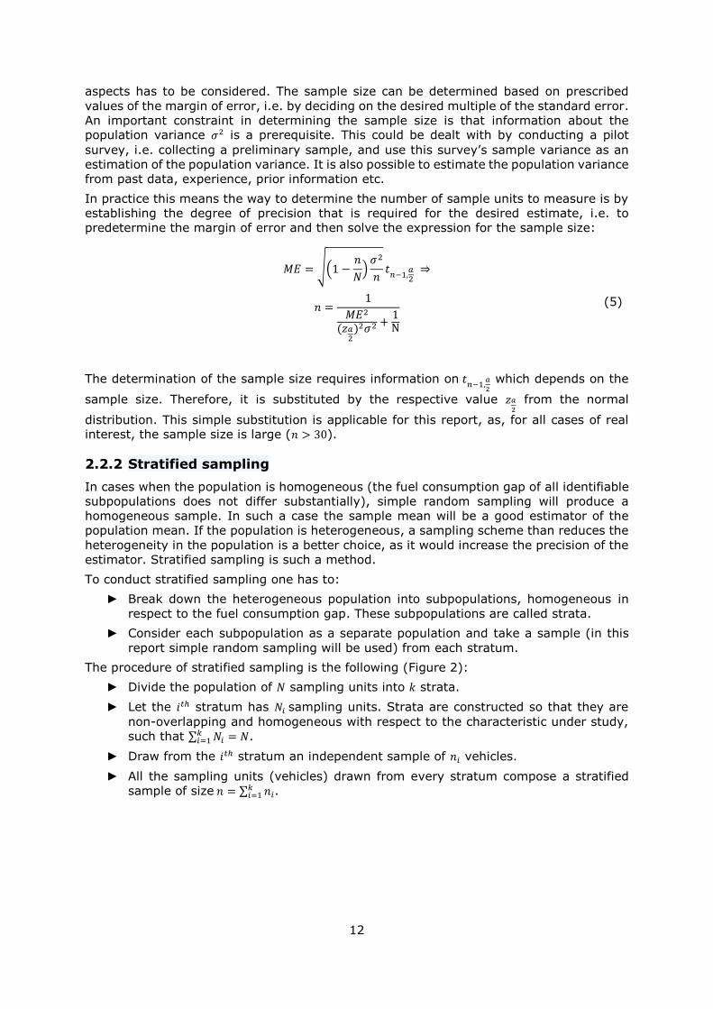
In practice this means the way to determine the number of sample units to measure is by

establishing the degree of precision that is required for the desired estimate, i.e. to

predetermine the margin of error and then solve the expression for the sample size:

𝑀𝐸 = √(1 −𝑛

𝑁)

𝜎2

𝑛𝑡

𝑛−1,𝑎2

⇒

𝑛 =1

𝑀𝐸2

(𝑧𝑎2

)2𝜎2 +1Ν

(5)

The determination of the sample size requires information on 𝑡𝑛−1,𝑎

2 which depends on the

sample size. Therefore, it is substituted by the respective value 𝑧𝑎

2 from the normal

distribution. This simple substitution is applicable for this report, as, for all cases of real interest, the sample size is large (𝑛 > 30).

2.2.2 Stratified sampling

In cases when the population is homogeneous (the fuel consumption gap of all identifiable

subpopulations does not differ substantially), simple random sampling will produce a

homogeneous sample. In such a case the sample mean will be a good estimator of the

population mean. If the population is heterogeneous, a sampling scheme than reduces the

heterogeneity in the population is a better choice, as it would increase the precision of the

estimator. Stratified sampling is such a method.

To conduct stratified sampling one has to:

► Break down the heterogeneous population into subpopulations, homogeneous in

respect to the fuel consumption gap. These subpopulations are called strata.

► Consider each subpopulation as a separate population and take a sample (in this

report simple random sampling will be used) from each stratum.

The procedure of stratified sampling is the following (Figure 2):

► Divide the population of 𝑁 sampling units into 𝑘 strata.

► Let the 𝑖𝑡ℎ stratum has 𝑁𝑖 sampling units. Strata are constructed so that they are

non-overlapping and homogeneous with respect to the characteristic under study,

such that ∑ 𝑁𝑖𝑘𝑖=1 = 𝑁.

► Draw from the 𝑖𝑡ℎ stratum an independent sample of 𝑛𝑖 vehicles.

► All the sampling units (vehicles) drawn from every stratum compose a stratified

sample of size 𝑛 = ∑ 𝑛𝑖𝑘𝑖=1 .

13

Figure 2 Stratifying sampling procedure

Source: JRC, 2021.

There are 𝑘 independent samples drawn through simple random sampling of sizes 𝑛1, … , 𝑛𝑘

from each stratum. Therefore, one can have 𝑘 estimators of the parameter (population

mean) based on these samples. The main goal is not to have 𝑘 different estimators of the

parameters but one single estimator. Taking into account that the final sample is a sum of 𝑘 independent samples, an unbiased estimator for the population mean is:

�̅�𝑠𝑡 = ∑

𝑁𝑖

𝑁

𝑘

𝑖=1

�̅�𝑖

(6)

where �̅�𝑖 is the sample mean from the 𝑖𝑡ℎ stratum.

An estimator of the standard error of the estimate �̅�𝑠𝑡 is:

𝑆𝐸(�̅�𝑠𝑡) = √∑ (𝑁𝑖

𝑁)

2

(1 −𝑛𝑖

𝑁𝑖

)

𝑘

𝑖=1

(𝑠𝑖

2

𝑛𝑖

) (7)

where the sample standard deviation 𝑠𝑖 is an unbiased estimator of the population standard

deviation 𝑆𝑖 of the 𝑖𝑡ℎ stratum.

Therefore the confidence interval for estimating the population mean is:

�̅�𝑠𝑡 ∓ 𝑀𝐸 = ∑

𝑁𝑖

𝑁

𝑘

𝑖=1

�̅�𝑖 ∓ √∑ (𝑁𝑖

𝑁)

2

(1 −𝑛𝑖

𝑁𝑖

)

𝑘

𝑖=1

(𝑠𝑖

2

𝑛𝑖

) 𝑡𝑑,

𝑎2

(8)

where 𝑑 is the Satterthwaite’s approximation for the degrees of freedom (Cochran 1977).

In the case of stratified sampling, as per the above formula, the precision of the estimator

depends on the following factors:

► The confidence lever or equivalently the allowable probability (α) that type I error

will occur.

► The stratification: The precision dependents on the strata sizes and most

importantly, the margin of error is small when the strata standard deviations are

small. This is suggestive of how to construct the strata. If all strata standard

deviations are small then the margin of error will also be small.

14

► The sample allocation: The total sample size has to be allocated among the strata.

Depending on the allocation, the precision varies.

► The total sample size: The higher the sample size the higher the precision of the

estimator.

Sample allocation methods are usually dependent on:

► the total number of vehicles in each stratum;

► the variability of the fuel consumption gap within each stratum;

► the cost of taking an observation from each stratum.

In this report, the cost of sampling from each stratum will be considered the same and

cost considerations will not be taken into account.

Three commonly used allocation procedures are:

1. Equal allocation: If the sizes of the strata are the same and there is no prior

information about the population, a legitimate decision would be to assume

equal sample sizes for the strata, so that:

𝑛𝑖 =𝑛

𝑘 1, … , 𝑘 (9)

2. Proportional allocation: if the sizes of the strata differ, proportional allocation

would usually be better in order to maintain a steady sampling fraction

throughout the population. The sample sizes per stratum are proportional to the

strata sizes:

𝑛𝑖 =𝑛

𝑁𝑁𝑖 1, … , 𝑘 (10)

3. Neyman allocation: In this allocation both the size and the variability in each

stratum are taken into account. Larger sample size is allocated to the larger and

more variable strata:

𝑛𝑖 =𝑛𝑁𝑖𝑆𝑖

∑ 𝑁𝑖𝑆𝑖𝑘𝑖=1

1, … , 𝑘 (11)

Choosing the sample size: Before calculating the sample size, the allocation method has

to be decided. The same way as in simple random sampling (section 2.2.1) the required

sample size is calculated by specifying the margin of error and confidence level in Equation (7). The determination of the sample size requires information on 𝑡𝑑,

𝑎

2 which itself

depends on the sample size. Therefore, it is substituted by the respective value 𝑧𝑎

2 from

the normal distribution.

► For equal allocation:

n =𝑘 ∗ ∑

𝑁𝑖2𝑆𝑖

2

N2𝑘𝑖=1

𝑀𝐸2

(𝑧𝑎2

)2 + ∑𝑁𝑖𝑆𝑖

2

N2𝑘𝑖=1

(12)

► for proportional allocation:

n =∑

𝑁𝑖𝑆𝑖2

N𝑘𝑖=1

𝑀𝐸2

(𝑧𝑎2


2

N2𝑘𝑖=1

(13)

► For Neyman allocation:

15

n =[∑

𝑁𝑖𝑆𝑖

𝑁𝑘𝑖=1 ]

2

𝑀𝐸2

(𝑧𝑎2


2

N2𝑘𝑖=1

(14)

Neyman allocation is a special case of optimal allocation which is formulated to minimize

the standard error of the estimate in Equation (7). This means that if the variances of the

strata are specified correctly, Neyman allocation will always, for the same sample size,

produce an estimator with a smaller variance than proportional allocation (Lohr 2019).

When the standard deviations of the strata are equal, Equation (13) and Equation (14) are

equivalent, which means that proportional and Neyman allocation requires the same

sample size. The degree of which Neyman allocation is better than proportional depends

on the variability of the strata standard deviations. In this report, the coefficient of variation

was used to quantify this variability.

If the strata sizes are large enough to permit the approximation 𝑁𝑖−1

𝑁𝑖≈ 1 then for the same

sample size proportional allocation always gives a smaller variance than simple random

sampling (Cochran 1977). This means that the required sample size to achieve the same

precision is smaller when using stratified sampling with proportional allocation. The degree

of which stratified sampling with a proportional allocation is better than simple random

sampling depends on how variable the strata means are. The higher the variability the

bigger the difference in required sample size. The coefficient of variation of the mean values

was used to quantify this variability.

To optimize the estimation of the fuel consumption gap one variable of interest: dependent

variable (the fuel consumption gap) and multiple stratification variables: independent

variables (see Table 1) were used. The methods which use one stratification variable are

called univariate stratification methods. If more than one stratification variables are utilized

they are called multivariate stratification methods. In this report cross-classification design

was used for multivariate stratification methods. In this design when L variables are used,

with the 𝑖𝑡ℎ having H𝑖 strata, they form H = ∏ H𝑖Li=1 strata.

Increasing the number of stratification variables makes the analysis more complicated and

strata with less than 2 vehicles may be formed. Equations (12) (13) and (14) which were

used for computing the sample sizes, require the strata standard deviations. Strata with

only one vehicle have no standard deviation. The approach used in this report was to join

strata with less than two vehicles into a superstratum. That is to say, this superstratum

contains all vehicles from strata with one vehicle. If there was only one stratum with one

vehicle, the vehicle was transferred to a random stratum.

2.2.3 Quota sampling

Quota sampling is a non-probability version of stratified sampling.

► In quota sampling, the entire population is divided into relevant strata using

stratification variables, like country or fuel type, chosen according to their relevance

to the fuel consumption gap.

► The number of vehicles that is sampled from each stratum is proportional to the

stratum’s vehicles, known from the EEA datasets. Thus, the sample is

representative of the entire population, in respect to the stratification variables.

► Convenience or judgment sampling is practiced to choose vehicles from each

stratum, both methods being subjective.

► By adhering to the stratification variables chosen, other factors contributing to

variability could lead to samples biased in certain ways. The resulting sample may

still have an unrepresentative combination of the stratification variables.

Understanding the variable under research (fuel consumption gap) and the factors

that contribute to its variability (fuel type, engine rated power, engine

displacement, manufacturer etc.) is important to design an accurate quota-

16

sampling scheme and avoid major bias. Interrelated controls can be used to attain

a correct combination of the stratification variables. A balance is desirable between

the higher costs of using more detailed quota controls and the increased

representativeness.

2.3 Data Sources

In this report four datasets are used, from which the three were user-based (Geco air,

Spritomonitor.de and Travelcard), while the fourth was the annual CO2 emissions

monitoring data from newly registered M1 vehicles in the EU in 2018 as reported by

Member States to the EEA.

► All datasets were utilized to test and validate the sampling methods. This was

accomplished by considering the datasets as the population, taking samples and

examining the accuracy and the required sample size for each method.

► Data from EEA were utilized to find the distributions/proportions of vehicles

registered in the EU in 2018 concerning other variables (e.g. per fuel type). These

were used for examining the representativeness of the user datasets.

► The user datasets were utilized to find trends, make comparisons and understand

the relation between the fuel consumption gap and the other available variables.

► The real-world data from the user datasets were also used to get information about

the fuel consumption gap, in particular its variability, which was required for

calculating sample sizes.

Data screening was applied to the three user-based datasets to remove faulty data, data

that were not in the scope of this report and to use comparable data from the different

datasets. Entries with the following characteristics were removed:

► Plug-in hybrid and electric vehicles.

► Vehicles not fuelled by diesel or petrol.

► Vehicles with either type-approval fuel consumption or type approval CO2 not

available.

► Vehicles with real-world fuel consumption less than or equal to 3 l/100km

(assumption that these are plug-in hybrid vehicles).

► Vehicles with type-approval, fuel consumption less than or equal to 3 l/100km

(assumption that these are plug-in hybrid vehicles).

► Vehicles with fuel consumption gap greater than 200%.

► Vehicles by manufacturers with only one vehicle in the dataset.

► Vehicles with registration-year other than 2018.

► Vehicles with a minimum recorded mileage (or in the case of Travelcard the number

of fuelling entries, because the distance was not available) less than a specified

distance (fuelling entry) criterion. For Geco air and Spritomonitor.de it was found

that vehicles with a driven distance less than 1,000 km and 1,250 km, respectively,

had to be removed to ensure there would be no statistically significant difference

when using vehicles with low recorded mileage. For Travelcard, vehicles with less

than three fuelling entries were excluded from the analysis.

17

Table 1 Available variables per dataset

Dataset

Variables Geco air (France)

Spritmonitor.de (Germany)

Travelcard

(Netherlands)

EEA

(EU)

Real-world FC or CO2 (l/100km or g/km)

✓ ✓ ✓ ✕

Type-approval FC or CO2 (l/100km or g/km)

✓ ✓ ✓ ✓

Fuel type ✓ ✓ ✓ ✓

Manufacturer ✓ ✓ ✓ ✓

Vehicle Year ✓ ✓ ✓ ✓

Engine Displacement (cc) ✓ ✕ ✓ ✓

Engine Rated Power (kW) ✓ ✓ ✓ ✓

Transmission Type ✓ ✓ ✕ ✕

Distance (1,000km) ✓ ✓ ✕ ✕

Number of fuelling events ✕ ✕ ✓ ✕

Country of registration ✕ ✕ ✓ ✓

Source: JRC, 2021.

2.3.1 Geco air

Geco air is a mobile application designed by IFP Energies Nouvelles to help individual users

become “eco-drivers” by estimating their pollutant (NOx and CO) and CO2 emissions. The

real-world CO2 emissions are calculated using a physical model that uses as inputs:

► The real-world data profiles of speed and altitude, which are calculated using the

GPS measurements, recorded at 1 Hz by the mobile phones;

► Technical specifications of the vehicle including those shown in Table 1, which are

either manually inserted by the user or extracted by the plate number (if it is

provided by the user). In the cases when the plate number is available, the type

approval CO2 value corresponds to the value appearing on the French registration

document.

IFP Energies Nouvelles provided JRC anonymized data of approximately 7,500 vehicles

registered from 1987 to 2019 (approximately 300 were registered in 2018) driven on real-

world conditions. For each vehicle, aggregated data were provided for both its CO2

emissions and the total distance, recorded via GPS, these data in addition to the provided

type approval CO2 emissions were used to derive the FC gap for every vehicle. Additionally,

the dataset included: fuel type, manufacturer, build year, engine displacement, engine

rated power and transmission type (Table 1).

After applying different selection criteria mentioned in section 2.3, a sample of 225 vehicles

remained. To ensure that the vehicles were driven for an adequate distance, all vehicles

with a recorded mileage less than 1,000 km were removed. This criterion of 1,000 km was

chosen because it was found that there is no statistically significant difference between the

subpopulations of vehicles driven for at least 1,000 km and at least 1,500 km. To find the

minimum distance that could be used, hypothesis tests were performed; it was checked

whether using shorter minimum driven distance would lead to a statistically significant difference to the mean value of the fuel consumption gap (𝑝𝑣𝑎𝑙𝑢𝑒 ≤ 0.05). The groups were

not normally distributed, therefore unpaired two-sample Wilcoxon test was used. Tietge et

al. (2019) used 1,500 km, and this was chosen as a reference and starting value and

compared to shorter distances. It was also confirmed that there was no statistically

significant difference between the subpopulation of vehicles driven for at least 1,500 km

18

and vehicles driven for longer distances. After applying the distance criterion a total of 127

vehicles were used for further analysis.

2.3.2 Spritmonitor.de

Spritmonitor.de is a free web service where owners of vehicles report real-world fuel

consumption. It was launched as a website in Germany in 2001, and aims to provide drivers

with a simple device to help them monitor their fuel consumption. To register a vehicle on

this website, the car owner provides vehicle specifications (i.e. fuel type, manufacturer,

built year, engine rated power and transmission type). Also, Spritmonitor.de users can

provide the type approval fuel consumption value and ’’trip’’ details with each entry. To

start making use of the service users are requested to fill the fuel tank completely, and the

first event provides the reference for calculations of fuel consumption. In every fuelling

entry, the user is requested to record the mileage and the liters fueled. Fuel consumption

data are added voluntarily, therefore there is a risk of self-selection bias.

Spritmonitor.de dataset had anonymized data on approximately 122,000 vehicles

registered from 2014 to 2019 (approximately 20,300 were registered in 2018). For every

vehicle, the real-world fuel consumption value was computed based on the total fuel

consumption of the vehicle and the total mileage. Using the same methodology as for Geco

air (section 2.3.1), and after applying the non-distance criteria 7,722 vehicles remained.

It was then calculated that the minimum mileage that would not produce statistically

significant differences was 1,250 km. Keeping only the vehicles with a recorded mileage

larger than 1,250 km, 7,218 were utilised in the analysis.

2.3.3 Travelcard

Travelcard Nederland B.V. is a fuel card provider based in the Netherlands. Fuel cards are

used as payment cards at gas stations and are employed by companies for tracing fuel

expenses of their fleets. The Travelcard data-providers are drivers who usually drive new

cars and change vehicles every few years. Usually, the expenses of Travelcard users are

covered by employers. Travelcard drivers may thus have a lower incentive to drive in a

fuel-conserving manner than private car owners. To compensate for this, Travelcard has a

fuel-cost saving program to push drivers to be mindful of excess fuel consumption. For

example, loyalty points are awarded to users with comparatively low fuel consumption and

a fuel pass that can be used in public transportation.

JRC received anonymized data for around 258,000 vehicles registered from 2011 to 2019

(approximately 28,300 were registered in 2018). The real-world and type-approval fuel

consumption was provided and used to calculate the fuel consumption gap. The dataset

also contained information about the fuel type, manufacturer, build year, engine

displacement, engine rated power transmission type and the number of fuelling events.

The data pre-processing by utilizing the same criteria as for Geco air and Spritmonitor.de

removed entries and 27,892 vehicles remained. Recorded mileage was not available and

the number of fuelling events was used instead. A similar methodology as in section 2.3.1

was applied to find that three was the minimum number of fuelling events which would not

lead to a significant difference for the average fuel consumption gap. Removing all vehicles

with less fuelling events resulted in a dataset consisting of 26,964 vehicles.

2.3.4 European Environment Agency

Regulation (EU) 2019/631 (previous (EC) No 443/2009) requires the Member States to

record information for each new passenger car registered in their territory. EEA documents

all the vehicles registered in the EU every year and provides public datasets with

anonymized data. These annual datasets include the type-approval CO2 emission, fuel

type, manufacturer, engine displacement, engine rated power, country of registration and

other information not used in this report. The EEA datasets do not include real-world CO2

emissions and fuel consumption, therefore the calculation of the fuel consumption gap was

not possible. For this report, the 2018 final dataset was used. It consists of approximately

15,273,000 passenger cars; after removing electrical and plug-in hybrid vehicles and

19

vehicles not fuelled by petrol or diesel, 14,623,747 remained. In this step, no other entries

were removed because of interest was to use this dataset to get a better understanding of

the census, hence removing vehicles because one variable was missing was not the suitable

approach.

The fuel consumption gap for EEA vehicles was simulated to apply the sampling methods

on the EEA dataset. The goal was to assign a reasonable fuel consumption gap that would

allow testing the sampling methods for the census (all the vehicles registered during one

year in the EU). The fuel consumption gap of Geco Air, Spritmonitor.de and Travelcard

vehicles were used to make a representative simulation (at least representative for

Germany, France and the Netherlands; in section 3.1 it is discussed whether these three

countries can represent the whole EU) of the fuel consumption gap for EEA’s vehicles. For

the simulation the following procedure was performed:

► A combined dataset consisting of vehicles sampled from Geco Air, Spritmonitor.de

and Travelcard was created. The number of vehicles sampled from Geco Air,

Spritmonitor.de and Travelcard datasets followed the same ratios, as the ratios of

vehicles registered, according to EEA dataset, in France (2,273,335), Germany

(3,303,367) and the Netherlands (381,689). All 127 vehicles of Geco Air dataset

were used, 185 from Spritmonitor.de and 21 from Travelcard were randomly

chosen.

► The combined and the EEA dataset were stratified in respect to five stratification

variables: the manufacturer, fuel type, type-approval CO2 emissions, engine rated

power and engine displacement.

► For every vehicle of the EEA dataset it was identified in which stratum it belonged.

If there were vehicles in the respective stratum of the combined dataset, the fuel

consumption gap was randomly sampled using the fuel consumption gap’s

distribution of that stratum of the combined dataset.

► If in the combined dataset there were no vehicles in that stratum, both datasets

were stratified in respect to four stratification variables: the manufacturer, fuel

type, type-approval CO2 emissions and engine rated power (removing the last

stratification variable). Then the stratum the vehicle belonged in respect to this

second stratification was identified. If the respective stratum of the combined

dataset had at least one vehicle, the fuel consumption gap was randomly sampled

from that stratum’s fuel consumption gap distribution. If not, the combined and the

EEA dataset were stratified in respect to three stratification variables: : the

manufacturer, fuel type and the type-approval CO2 emissions and the same

procedure was repeated.

► This continued until a fuel consumption gap was assigned for that vehicle (reducing

by one the stratification variables, until the stratification was done only by one

stratification variable: the manufacturer). If there were no vehicles of that

manufacturer in the combined dataset, a new stratification using four stratification

variables: the type-approval CO2 emissions, fuel type, engine rated power and

engine displacement was performed. The procedure was repeated until a fuel

consumption gap was assigned. The last possible stratification was by one

stratification variable: the type-approval CO2 emissions, in which case a value is

always assigned.

20

3 Data analysis

3.1 Dataset Representativeness

To evaluate the datasets used for testing the sampling methods utilised to support the

determination of the fuel consumption gap of vehicles registered in the EU after 2021, it

was investigated whether:

► The three datasets were representative of the fleet of EU vehicles registered in

2018;

► The three datasets were representative of the sub-fleets of their respective

countries (Geco air for France, Sprtimonitor.de for Germany and Travelcard for the

Netherlands);

► These three countries could represent the 2018 population of newly registered

vehicles in the EU.

Representativeness was determined in respect to fuel type, type approval CO2 emissions,

vehicle manufacturer, engine rated power and engine displacement.

The distribution of the whole fleet of vehicles introduced in the EU market in 2018 was

calculated from the EEA dataset, for the manufacturer, type-approval CO2 emissions

(g/km), fuel type, engine displacement (cc) and engine power (kW). The distributions of

the country-wise sub-fleets were collected for the above five variables. For the same

variables, the distribution was calculated of the Geco Air, Spritmonitor.de and Travelcard

datasets.

For each of the five variables, plots were drawn where Geco Air, Spritmonitor.de and

Travelcard were compared to the French, German and Dutch sub-fleets, respectively, as

well as to the 2018 European fleet. It should be noted that the following analysis does not

represent the whole Geco Air, Spritmonitor.de and Travelcard datasets, but only those

registered in 2018 and those that passed the removal criteria as described in section 2.3.

The main purpose of this section was not to evaluate the datasets but to check whether,

and to what degree, it is justified to use them for getting a valid indication of the fuel

consumption gap across the EU. The datasets cannot be used in the context of Regulation

(EU) 2019/631 as they are not relying on data recorded using OBFCM devices.

Fuel type is a critical parameter concerning the type-approval and the real-world fuel

consumption and subsequently the FC gap. These relationships have been studied in

(Ntziachristos et al. 2014). For the three user datasets used in this report, results are

presented in Figure 3. The relative frequencies are larger than the corresponding ones that

would be calculated if all vehicles were used. Nevertheless, this does not influence the

inferences made in this report. Variations exist from country to country. The share of newly

registered diesel and petrol vehicles in 2018 for the German and French market is close to

the share of the whole EU (Figure 3), while in the Netherlands in 2018 only 12.5% of the

newly registered vehicles were diesel. Hence, the Netherlands subpopulation cannot

represent the whole EU when it comes to fuel type.

In Geco Air dataset approximately 58.0% of the vehicles were diesel-powered. This is a

substantial difference compared to EEA (37.8%) and EEA France (41.5%). 22.0% of

Spritmonitor.de vehicles were diesel-powered, which is relatively closer to the German

sub-fleet’s share (32.6%). For Travelcard, almost 42.0% of the vehicles used diesel fuel,

therefore this dataset cannot be considered as representative of the Dutch fleet in respect

to fuel type, but it is representative of the whole European fleet.

21

Figure 3 Representativeness of datasets per fuel type

Source: JRC, 2021.

Figure 4 presents all manufacturers that have a share of a least 2% on the respective

dataset. The French sub fleet is not representative of the whole European fleet, because

Renault, Peugeot and Citroen share almost 50% of the French market, while their portion

of the whole EU fleet is less than 26%. In Germany there is a similar situation, e.g. Audi,

BMW, Mercedes-Benz and Volkswagen have a higher share of the German market (46%)

in comparison to their share in the European fleet (28%). The Dutch sub-fleet exhibits the

best behaviour, only two manufacturers have a difference greater than 2% (Opel and Kia).

Geco Air dataset is representative of the French market, except for Peugeot which is

overrepresented by 14% in Geco air and Renault which is underrepresented by 9% in Geco

air. Spritmonitor.de is not representing satisfactorily neither the German sub fleet nor the

European one. Travelcard is over-representing the most popular manufacturers, reaching

up to 7% for Volkswagen.

22

Figure 4 Representativeness of datasets per manufacturer

Source: JRC, 2021.

The CO2 emission gap and consequently the fuel consumption gap is a function of the real-

world and the type-approval CO2 emissions. In some cases linear relationships can be found

and simple linear regression models can be constructed for predicting the real-world fuel

consumption only by using the type-approval fuel consumption (Ntziachristos et al. 2014).

The French and Dutch sub-fleets (Figure 5) have more vehicles with low type-approval CO2

emissions in comparison to the whole fleet. On the other hand in the German market the

percentage of vehicles with high type-approval CO2 emissions sold in 2018 was higher than

the respective one of the whole EU market.

Figure 5 Representativeness of datasets per type-approval CO2

Source: JRC, 2021.

23

Concerning type-approval CO2 emissions, Geco Air’s density distribution was relatively

close to both EEA France’s and EEA’s distributions. Vehicles of Spritmonitor.de with type-

approval emissions around 110g/km were overrepresented. Travelcard was the best

representative of the EU fleet with respect to type-approval CO2 emissions.

Vehicles sold in France in 2018 had on average lower engine rated power compared to the

average across the EU, while in Germany it was higher. The Dutch market was closer to

the whole European as regards engine rated power (Figure 6).

In Geco air dataset the engine rated power was closer to the whole fleet’s compared to the

French fleet’s. Spritmonitor.de approximates well the German market, with the only

exception being vehicles with engine rated power around 110kW. Travelcard is relatively

close to the Dutch sub-fleet.

Figure 6 Representativeness of datasets per engine rated power

Source: JRC, 2021.

Engine displacement was not available for Spritmonitor.de vehicles. Both the French and

Dutch vehicle’s average engine displacement in 2018 were lower than across Europe.

Worth mentioning is that in 2018, the Netherlands had the lowest average engine

displacement in the EU for new passenger car registrations. Travelcard is representative of

the Netherland’s situation in all but for vehicles with low engine displacement (Figure 7).

Figure 7 Representativeness of datasets per engine displacement

Source: JRC, 2021.

24

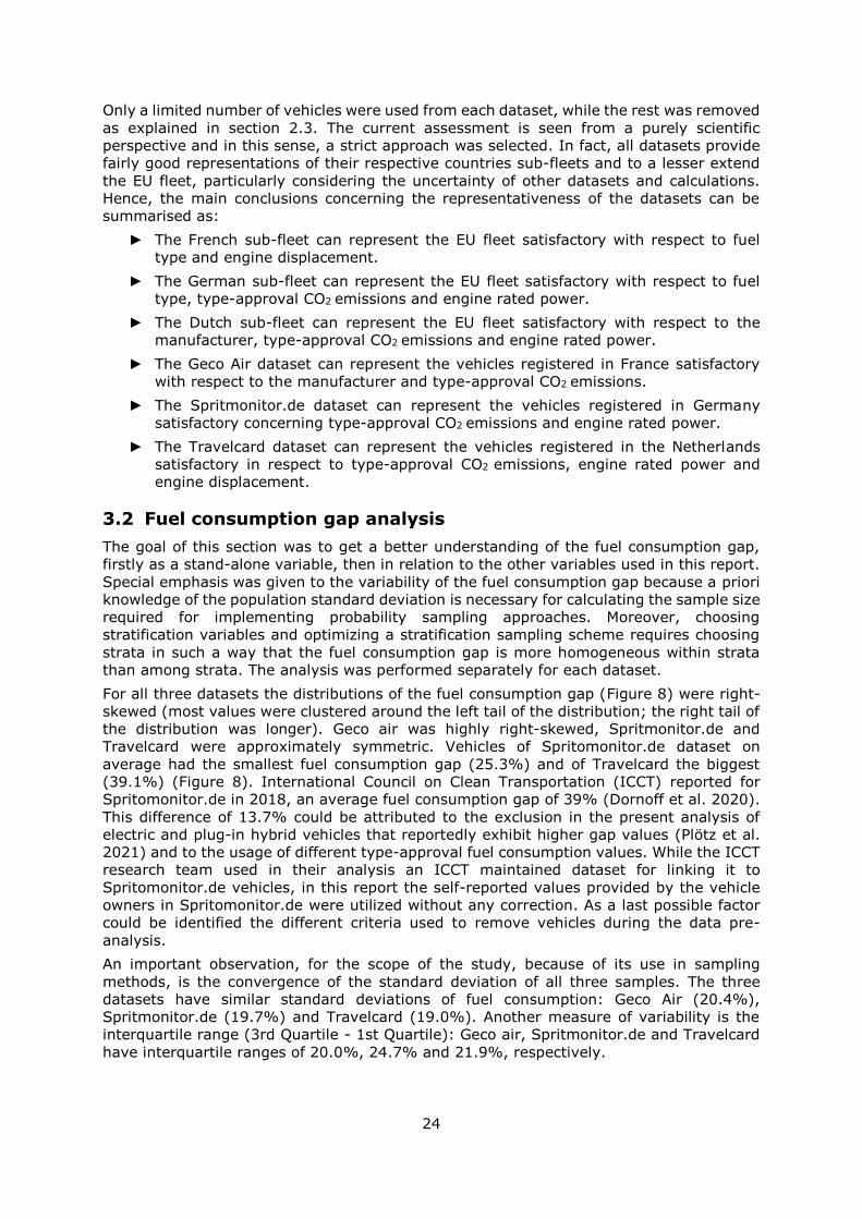
Only a limited number of vehicles were used from each dataset, while the rest was removed

as explained in section 2.3. The current assessment is seen from a purely scientific

perspective and in this sense, a strict approach was selected. In fact, all datasets provide

fairly good representations of their respective countries sub-fleets and to a lesser extend

the EU fleet, particularly considering the uncertainty of other datasets and calculations.

Hence, the main conclusions concerning the representativeness of the datasets can be

summarised as:

► The French sub-fleet can represent the EU fleet satisfactory with respect to fuel

type and engine displacement.

► The German sub-fleet can represent the EU fleet satisfactory with respect to fuel

type, type-approval CO2 emissions and engine rated power.

► The Dutch sub-fleet can represent the EU fleet satisfactory with respect to the

manufacturer, type-approval CO2 emissions and engine rated power.

► The Geco Air dataset can represent the vehicles registered in France satisfactory

with respect to the manufacturer and type-approval CO2 emissions.

► The Spritmonitor.de dataset can represent the vehicles registered in Germany

satisfactory concerning type-approval CO2 emissions and engine rated power.

► The Travelcard dataset can represent the vehicles registered in the Netherlands

satisfactory in respect to type-approval CO2 emissions, engine rated power and

engine displacement.

3.2 Fuel consumption gap analysis

The goal of this section was to get a better understanding of the fuel consumption gap,

firstly as a stand-alone variable, then in relation to the other variables used in this report.

Special emphasis was given to the variability of the fuel consumption gap because a priori

knowledge of the population standard deviation is necessary for calculating the sample size

required for implementing probability sampling approaches. Moreover, choosing

stratification variables and optimizing a stratification sampling scheme requires choosing

strata in such a way that the fuel consumption gap is more homogeneous within strata

than among strata. The analysis was performed separately for each dataset.

For all three datasets the distributions of the fuel consumption gap (Figure 8) were right-

skewed (most values were clustered around the left tail of the distribution; the right tail of

the distribution was longer). Geco air was highly right-skewed, Spritmonitor.de and

Travelcard were approximately symmetric. Vehicles of Spritomonitor.de dataset on

average had the smallest fuel consumption gap (25.3%) and of Travelcard the biggest

(39.1%) (Figure 8). International Council on Clean Transportation (ICCT) reported for

Spritomonitor.de in 2018, an average fuel consumption gap of 39% (Dornoff et al. 2020).

This difference of 13.7% could be attributed to the exclusion in the present analysis of

electric and plug-in hybrid vehicles that reportedly exhibit higher gap values (Plötz et al.

2021) and to the usage of different type-approval fuel consumption values. While the ICCT

research team used in their analysis an ICCT maintained dataset for linking it to

Spritomonitor.de vehicles, in this report the self-reported values provided by the vehicle

owners in Spritomonitor.de were utilized without any correction. As a last possible factor

could be identified the different criteria used to remove vehicles during the data pre-

analysis.

An important observation, for the scope of the study, because of its use in sampling

methods, is the convergence of the standard deviation of all three samples. The three

datasets have similar standard deviations of fuel consumption: Geco Air (20.4%),

Spritmonitor.de (19.7%) and Travelcard (19.0%). Another measure of variability is the

interquartile range (3rd Quartile - 1st Quartile): Geco air, Spritmonitor.de and Travelcard

have interquartile ranges of 20.0%, 24.7% and 21.9%, respectively.

25

Figure 8 Histograms & statistics of fuel consumption gap, per dataset

Source: JRC, 2021.

The relationship between the fuel consumption gap and fuel type presents similar patterns

in all three datasets (Figure 9). Petrol vehicles had on average lower fuel consumption gap,

however, there was no statistically significant difference. Concerning the variability of the

fuel consumption gap for Spritmonitor.de and Travelcard there was no statistically

significant difference between diesel and petrol vehicles (e.g. for Travelcard the standard

deviation of the fuel consumption gap for diesel and petrol vehicles was 18.8% and 18.9%,

respectively. The IQR was 21.5% in both groups). Geco air petrol fuelled vehicles had a

substantially larger standard deviation compared to the diesel powered ones (27.6%-

13.4%). The reason is that in Geco air there were quite a few petrol vehicles with high fuel

consumption gap and these ‘outliers’, not presented in Figure 9, strongly affected the

standard deviation.

Vehicles with a manual transmission had a lower average and lower variability of the fuel

consumption gap in both Geco air and Spritmonitor.de datasets (Figure 9).

Figure 9 Fuel consumption gap by fuel type and transmission type, per dataset. Red triangles

depict the mean values

Source: JRC, 2021.

26

The three datasets give different results concerning the average and the standard deviation

of the fuel consumption gap per manufacturer (Figure 10). In Spritmonitor.de the averages

and the variabilities of the fuel consumption gap per manufacturer, do not present very

large variations. The largest variations are seen in Geco air dataset, followed by Travelcard.

In Figure 11, the relation between the fuel consumption gap and the type-approval CO2

emission, the engine rated power and the engine displacement are presented for each

dataset. The curves are an estimate of the conditional mean function, i.e. it is an estimate

of the mean fuel consumption gap conditional on the variable shown on the x-axis. For

Geco air, which had less than 1,000 vehicles, locally estimated scatterplot smoothing was

applied. For Spritmonitor.de and Travelcard a generalized additive model was fitted to the

data.

Travelcard and Spritomonitor.de vehicles with low type-approval CO2 emissions had in

average the largest fuel consumption gap. For Spritmonitor.de an almost linear decreasing

relationship was observed between the average fuel consumption gap and the type-

approval CO2 emissions. For Travelcard the average fuel consumption gap decreased until

approximately 140g/km and then presented a slight increase. For Geco air vehicles with

low and high type-approval CO2 emissions had the lowest average fuel consumption gap.

Figure 10 Fuel consumption gap by manufacturer, per dataset. Only manufacturers with at least a

share of 4% in one of the datasets are presented. Red triangles depict the mean values

Source: JRC, 2021.

In all three datasets, the average fuel consumption did not present big divergences for

vehicles with an engine rated power higher than 125 kW. Geco air and Spritmonitor.de

vehicles had an average higher fuel consumption gap for vehicles with a lower engine rated

power. The opposite held true for Travelcard vehicles.

Geco air and Travelcard presented similar trends in regards to the relationship between

the average fuel consumption and engine displacement. In both datasets, there were no

big variations in the vehicles average fuel consumption gap concerning the engine

displacement. Vehicles with low and high engine displacement had a slightly higher fuel

consumption gap.

The average fuel consumption of Geco air vehicles was low for vehicles with low mileage.

For Spritmonitor.de, vehicles with a high mileage had in average a lower fuel consumption

gap.

27

Figure 11 Average fuel consumption gap in relation to type-approval CO2 emissions, engine rated

power, engine displacement and distance driven, per dataset

Source: JRC, 2021.

3.3 Validation of sampling methods

3.3.1 Simple random sampling

For the simple random sampling analysis, the only variable used was the fuel consumption

gap (Table 2). The population sizes and the population mean values differ substantially,

allowing an understanding of the impact they have on the required sample size. The

standard deviations are similar; nevertheless, the impact on the sample size is shown in

Figure 12. The mean value of the fuel consumption gap of EEA vehicles lies between the

minimum and the maximum of the other three datasets, the standard deviation is larger.

This is a consequence of the way EEA vehicles fuel consumption gap was simulated using

the other three datasets vehicles’ fuel consumption gap (section 2.3.4).

A preliminary estimation of the required sample size, in case of simple random sampling,

for a population of 15 million vehicles and population standard deviation ranging from 0%

to 75% is presented in Figure 12. The most stringent requirements for the precision

examined in this report (confidence level 99% and margin of error 1%) were adopted. The

three user-based datasets examined in this report had a standard deviation of the fuel

consumption gap approximately 20% (Figure 8). For a standard deviation of 20%, the

required sample size is 2,654. If the standard deviation was 25% the sample size would

be 4,146 vehicles. Even if the population standard deviation is 75%, a sample size of less

than 38,000 (0.25% of the total population) vehicles would be enough to reach the

required precision.

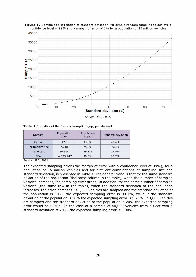
28

Figure 12 Sample size in relation to standard deviation, for simple random sampling to achieve a

confidence level of 99% and a margin of error of 1% for a population of 15 million vehicles

Source: JRC, 2021.

Table 2 Statistics of the fuel consumption gap, per dataset

Dataset Population

size Population

mean Standard deviation

Geco air 127 33.3% 20.4%

Spritmonitor.de 7,218 25.3% 19.7%

Travelcard 26,964 39.1% 19.0%

EEA 14,623,747 30.5% 20.7%

Source: JRC, 2021.

The expected sampling error (the margin of error with a confidence level of 99%), for a

population of 15 million vehicles and for different combinations of sampling size and

standard deviation, is presented in Table 3. The general trend is that for the same standard

deviation of the population (the same column in the table), when the number of sampled

vehicles increases, the sampling error drops. In addition, for the same number of sampled

vehicles (the same raw in the table), when the standard deviation of the population

increases, the error increases. If 1,000 vehicles are sampled and the standard deviation of

the population is 10%, the expected sampling error is 0.81%, while if the standard

deviation of the population is 70% the expected sampling error is 5.70%. If 3,000 vehicles

are sampled and the standard deviation of the population is 20% the expected sampling

error would be 0.94%. In the case of a sample of 40,000 vehicles from a fleet with a

standard deviation of 70%, the expected sampling error is 0.90%

29

Table 3 Margin of error in relation to sample size and standard deviation, for simple random

sampling for a population of 15 million vehicles

Sample Size

Standard Deviation

10% 20% 30% 40% 50% 60% 70%

1,000 0.81 1.63 2.44 3.26 4.07 4.89 5.70

2,000 0.58 1.15 1.73 2.30 2.88 3.46 4.03

3,000 0.47 0.94 1.41 1.88 2.35 2.82 3.29

4,000 0.41 0.81 1.22 1.63 2.04 2.44 2.85

5,000 0.36 0.73 1.09 1.46 1.82 2.19 2.55

6,000 0.33 0.66 1.00 1.33 1.66 1.99 2.33

7,000 0.31 0.62 0.92 1.23 1.54 1.85 2.15

8,000 0.29 0.58 0.86 1.15 1.44 1.73 2.02

9,000 0.27 0.54 0.81 1.09 1.36 1.63 1.90

10,000 0.26 0.51 0.77 1.03 1.29 1.54 1.80

20,000 0.18 0.36 0.55 0.73 0.91 1.09 1.27

30,000 0.15 0.3 0.45 0.59 0.74 0.89 1.04

40,000 0.13 0.26 0.39 0.51 0.64 0.77 0.90

Note: confidence level 99%; in bold the lowest sample sizes to achieve a margin of error less than 1% for each population standard deviation

Source: JRC, 2021.

To calculate the required sample size and to validate the accuracy of the simple random

sampling method for every dataset, the following procedure was performed:

► For each combination between the margin of error (10%, 9%, to 1%) and

confidence level (90%, 95% and 99%), Equation (5) was used to calculate the

required sample size (Table 4).

► For every resulting sample size, one million random samples were simulated

► For every random sample, the following were calculated:

o The sample mean and the sampling error (the difference between the

sampling and the population mean);

o It was examined whether the absolute value of the sampling error was lower

than the required margin of error;

o For each combination of the margin of error and confidence level, the

percentage of the cases for which the absolute value of the sampling error

was lower than the specified margin of error was calculated (Table 5);

► Finally, these percentages were compared to the respective confidence level.

For example for Geco air, to achieve MΕ = 1% and cl = 99% a sample size of 𝑛 = 122 was

required. One million samples of 122 vehicles were randomly simulated. Of these samples,

the population mean was predicted accurately 990079 times (99%). 99% is the percentage

of the number of times the absolute sampling error was lower than the margin of error, or

equivalently the percentage of the number of times the sample mean was inside the

interval (Figure 13):

(𝑚𝑒𝑎𝑛𝑝𝑜𝑝 − 𝑀𝐸 , 𝑚𝑒𝑎𝑛𝑝𝑜𝑝 + 𝑀𝐸) = (33.3 − 1, 33.3 + 1) = (32.3, 34.3)

The sampling method was validated in this case, because 99 % ≥ 𝑐𝑙 = 99%.

30

Table 4 Sample size required per dataset for different margins of error and confidence levels, for

simple random sampling

Dataset 𝒄𝒍 𝚳𝚬

10% 9% 8% 7% 6% 5% 4% 3% 2% 1%

Geco air

90% 11 13 16 20 26 34 46 64 88 115

95% 15 18 21 27 33 43 57 75 97 118

99% 23 27 33 40 48 60 74 90 108 122

Spritmonitor.de

90% 11 13 17 22 30 42 66 115 254 9157

95% 15 19 24 31 42 60 92 162 355 1,236

99% 26 32 40 53 71 102 158 276 591 1,898

Travelcard

90% 10 13 16 20 28 39 61 108 242 942

95% 14 18 22 29 39 56 87 154 342 1,318

99% 24 30 38 49 67 96 149 264 586 2,198

EEA

90% 12 15 19 24 33 47 73 130 291 1,163

95% 17 21 26 34 46 67 104 184 413 1,654

99% 29 36 45 59 80 115 179 317 713 2,851

Source: JRC, 2021.

Four factors contribute to the sample size. Two depend on the demanded accuracy: the

confidence level and the margin of error. The other two are population parameters, the

population size and the population standard deviation.

The calculated sample sizes for all four datasets (Table 4) confirm that the required sample

size increases as the demanded confidence level increases and as the margin of error

decreases. For example for Geco air, to achieve confidence level 90% and margin of error

10%, 11 vehicles were required. If the confidence level remained at 90%, while the

requested margin of error was 1%, 115 vehicles would need to be sampled. In the most

stringent case examined in this report, of confidence level, 99% and margin of error 1%,

122 of the total 127 vehicles would have to be sampled.

Concerning the population parameters, it holds that for both, the population size and the

population standard deviation the larger they are, the larger the required sample size is.

This is clear when comparing results for Travelcard and EEA datasets: EEA has a larger

population size and population standard deviation, and for the same confidence level and

margin of error, the required sample size for EEA is larger for all cases compared to

Travelcard. On the other hand Spritmonitor.de has a smaller population size, but a higher

population standard deviation than Travelcard. Consequently, for the same confidence

level and margin of error, the required sample size for Spritmonitor.de is sometimes lower

and sometimes higher than the required sample size for Travelcard. For example, for

confidence level 99% and margin of error 10% 26 and 24 vehicles are respectively required

from the datasets of Spritmonitor.de and Travelcard. For confidence level 99% and margin

of error 1%, 1,898 and 2,198 vehicles are required for Spritmonitor.de and Travelcard

respectively. The reason for that can be derived from Equation (5), the confidence level

and the margin of error can be considered as weights for the population size and the

population standard deviation. The standard deviation is multiplied by ME2

(za2

)2, therefore the

higher this weight is the bigger the contribution of the standard deviation. This weight is

higher for a larger margin of error and lower confidence level. This explains why for a large

margin of error and low confidence level Spritmonitor.de needs more vehicles to reach the

same accuracy as Travelcard.

As a final note, it should be mentioned that while the required sample size increases as the

population size increases, there is a limit: after a certain point no matter how much the

population size increases the increase of the required sample size is negligible. This

behaviour is visible when looking at the datasets in Table 4, for confidence level 99% and

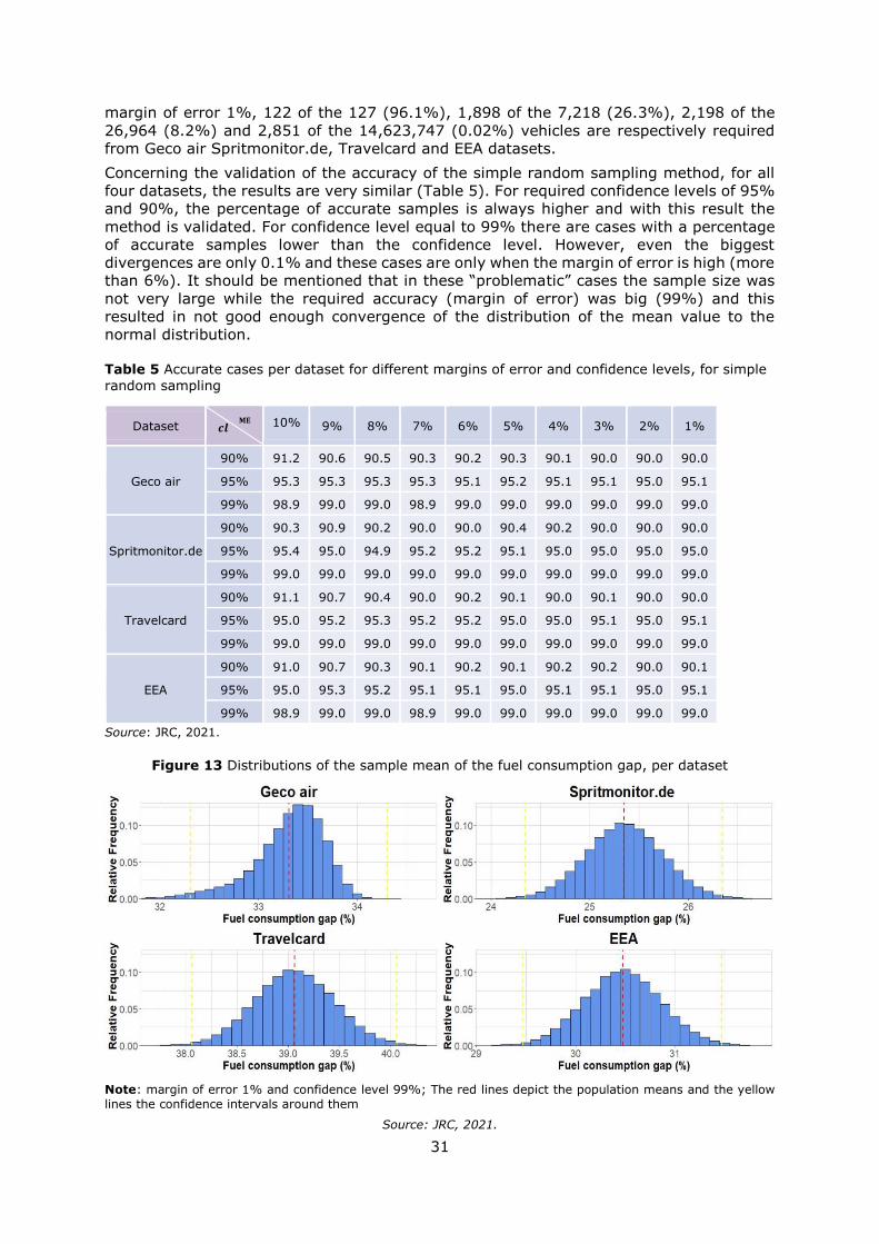
31

margin of error 1%, 122 of the 127 (96.1%), 1,898 of the 7,218 (26.3%), 2,198 of the

26,964 (8.2%) and 2,851 of the 14,623,747 (0.02%) vehicles are respectively required

from Geco air Spritmonitor.de, Travelcard and EEA datasets.

Concerning the validation of the accuracy of the simple random sampling method, for all

four datasets, the results are very similar (Table 5). For required confidence levels of 95%

and 90%, the percentage of accurate samples is always higher and with this result the

method is validated. For confidence level equal to 99% there are cases with a percentage

of accurate samples lower than the confidence level. However, even the biggest

divergences are only 0.1% and these cases are only when the margin of error is high (more

than 6%). It should be mentioned that in these “problematic” cases the sample size was

not very large while the required accuracy (margin of error) was big (99%) and this

resulted in not good enough convergence of the distribution of the mean value to the

normal distribution.

Table 5 Accurate cases per dataset for different margins of error and confidence levels, for simple

random sampling

Dataset 𝒄𝒍 𝐌𝐄

10% 9% 8% 7% 6% 5% 4% 3% 2% 1%

Geco air

90% 91.2 90.6 90.5 90.3 90.2 90.3 90.1 90.0 90.0 90.0

95% 95.3 95.3 95.3 95.3 95.1 95.2 95.1 95.1 95.0 95.1

99% 98.9 99.0 99.0 98.9 99.0 99.0 99.0 99.0 99.0 99.0

Spritmonitor.de

90% 90.3 90.9 90.2 90.0 90.0 90.4 90.2 90.0 90.0 90.0

95% 95.4 95.0 94.9 95.2 95.2 95.1 95.0 95.0 95.0 95.0

99% 99.0 99.0 99.0 99.0 99.0 99.0 99.0 99.0 99.0 99.0

Travelcard

90% 91.1 90.7 90.4 90.0 90.2 90.1 90.0 90.1 90.0 90.0

95% 95.0 95.2 95.3 95.2 95.2 95.0 95.0 95.1 95.0 95.1

99% 99.0 99.0 99.0 99.0 99.0 99.0 99.0 99.0 99.0 99.0

EEA

90% 91.0 90.7 90.3 90.1 90.2 90.1 90.2 90.2 90.0 90.1

95% 95.0 95.3 95.2 95.1 95.1 95.0 95.1 95.1 95.0 95.1

99% 98.9 99.0 99.0 98.9 99.0 99.0 99.0 99.0 99.0 99.0

Source: JRC, 2021.

Figure 13 Distributions of the sample mean of the fuel consumption gap, per dataset

Note: margin of error 1% and confidence level 99%; The red lines depict the population means and the yellow

lines the confidence intervals around them

Source: JRC, 2021.

32

Some statistics of the difference between the sample mean and the population mean (𝑚𝑒𝑎𝑛𝑠𝑎𝑚 − 𝑚𝑒𝑎𝑛𝑝𝑜𝑝) for confidence level 99% and margin of error 1%, for the four datasets

are presented in Table 6. For all datasets, except Geco air which has a small population

size the differences have symmetrical distributions (Figure 13) with mean and median 0.0

and standard deviation 0.4. Half the differences (50%) are between -0.3% and 0.3%, while

99% are between -1% and 1%. The maximum and minimum difference are less than ±2%,

denoting that in even the worst (less accurate) sample, the sampling error was less than

2%.

Table 6 Sampling error per dataset for margin of error 1% and confidence level 99%, for simple random sampling

Dataset Minimum

(%)

1st Quartile

(%)

Median (%)

Mean

(%)

3rd Quartile

(%)

Maximum (%)

Standard Deviation (%)

Geco air -1.9 -0.3 0.0 0.0 0.3 1.5 0.4

Spritmonitor.de -1.8 -0.3 0.0 0.0 0.3 1.7 0.4

Travelcard -1.6 -0.3 0.0 0.0 0.3 1.7 0.4

EEA -1.6 -0.3 0.0 0.0 0.3 1.6 0.4

Source: JRC, 2021.

3.3.2 Stratified sampling

In stratified sampling, the first step required is to choose the stratification variable(s) and

to determine the strata to split the population. In this section, different stratification

variables were examined and conclusions and comparisons are presented. The main goal

was to get a better understanding of the variables which require the smallest sample size

to predict accurately the fuel consumption gap of the population. Additionally to identify

the variables that are relevant to the fuel consumption gap, which were used to construct

a quota sampling scheme. For each dataset, variables presented in Table 1 were used, first

separately (univariate stratification) and then in combinations (multivariate stratification).

To calculate the required sample size, allocate it to the strata, and validate the accuracy

of the stratified sampling method, for Geco air, Spritmonitor.de, Travelcard and EEA

datasets, the following analysis was performed:

► One or more stratification variables were chosen;

► For each combination of the margin of error (10%, 9% to 1%) and confidence level

(90%, 95%, 99%), the required sample size was calculated;

► This sample size was allocated to the k strata after applying different allocation

methods;

► For equal allocation, if the sampling size required from a stratum was higher than

the stratum size, the method was termed as unfeasible;

► For proportional and for Neyman allocation, reallocations were performed to ensure

that the number of sampling units to be drawn from all strata were not more than

the number of sampling units in the stratum:

ni ≤ 𝑁i, 𝑖 = 1, … , 𝑘

► For every resulting sample size, million (𝑛𝑠𝑖𝑚 = 1,000,000) random samples were

simulated.

► For every sample the following was calculated:

o The sample mean;

33

o The sampling error (the difference between the sampling and the population

mean);

o It was examined whether the absolute value of the sampling error was

larger than the margin of error.

► The percentage of the cases for which the absolute value of the sampling error was

lower than the specified margin of error was calculated for each combination of the

margin of error and confidence level.

► Finally, these percentages were compared to the respective required confidence

levels and the method was validated.

The sample sizes for Neyman (𝑛𝑜), proportional (𝑛𝑝), and equal allocation (𝑛𝑒), without

considerations of the sampling cost, were calculated using Equations (14), (13) and (12)

respectively. The parameters contributing to the sample size are related to the demanded

accuracy, population and stratification. The confidence level and the margin of error

determine the accuracy. Concerning the population parameters, the population size and

the population standard deviation influence the sample size. The population standard deviation (𝑆) is not directly used, the contribution to the sample size depends on the strata

standard deviations (𝑆𝑖). The importance of the stratification can be also seen from the use

of the strata size𝑠 (𝑁𝑖), and in the case of equal allocation the number of strata (k) in the

formulas.

The sample size allocation for equal, proportional and Neyman allocation was performed,

using Equations (9), (10) and (11) respectively. For equal allocation, when the results were

not integers, they were rounded up to the next integer and the required sample size was

recalculated. For proportional and Neyman allocation controlled rounding was used to

round these real values to a set of integers that sum to the calculated sample sizes.

Detailed analysis and explanations for univariate stratification stratifying by the fuel type

and the type-approval CO2 emissions are provided in sections 3.3.2.1 and 3.3.2.2,

respectively. Results of these two sections were used to compare the different allocation

procedures. Based on the results of section 3.3.2.1 and the simple random analysis of

section 3.3.1 it was decided for the analysis that follows to use a confidence level of 99%

and a margin of error of 1%. To avoid repeatable and almost identical tables and

conclusions, validation results for stratification sampling are presented only in section

3.3.2.1. In section 3.3.2.3 the stratification variables are compared separately. Multivariate

stratification is introduced in section 3.3.2.4, combining variables of interest. In section

3.3.2.5 the sample sizes are presented when accurate estimators are also required per

stratum.

Stratifying by Fuel Type

A simple univariate stratification is when stratifying by fuel type, in the sense that the

populations (Geco air, Spritmonitor.de, Travelcard and EEA) were split into only two strata

(diesel and petrol vehicles). Geco air had more diesel vehicles than petrol vehicles (58.3%-

41.7%), the standard deviation of the fuel consumption gap was lower for diesel vehicles

(13.4%-27.6%) (Table 7). Spritmonitor.de had less than one third diesel than petrol

vehicles (22.0%-78.0%), standard deviation was slightly higher for the diesel vehicles

(20.0%-19.5%). Travelcard had a higher number of petrol vehicles (58.1%-41.9%), the

two strata had almost the same standard deviation (18.9%-18.8%). EEA also had more

petrol vehicles (62.2%-37.8%), the standard deviation of the simulated fuel consumption

gap was higher for petrol vehicles (23.4%-15.2%).

34

Table 7 Fuel consumption gap grouped by fuel type, per dataset

Dataset

Fuel type Geco air Spritmonitor.de Travelcard EEA

𝑁𝑖 𝑚𝑖 𝑠𝑑𝑖 𝑁𝑖 𝑚𝑖 𝑠𝑑𝑖 𝑁𝑖 𝑚𝑖 𝑠𝑑𝑖 𝑁𝑖 𝑚𝑖 𝑠𝑑𝑖

Diesel 74 33 13.4 1,586 28.2 20.0 11,296 41.6 18.8 5,530,321 32.1 15.2

Petrol 53 33.7 27.6 5,632 24.5 19.5 15,668 37.3 18.9 9,093,426 29.5 23.4

Minimum 53 33 13.4 1,586 24.5 19.5 11,296 37.3 18.8 5,530,321 29.5 15.2

Maximum 74 33.7 27.6 5,632 28.2 20.0 15,668 41.6 18.9 9,093,426 32.1 23.4

Mean 63.5 33.4 20.5 3,609 26.4 19.8 13,482 39.5 18.9 7,311,873.5 30.8 19.3

Standard deviation

14.8 0.5 10 2,861 2.6 0.3 3,091.5 3.0 0.1 2,519,495.7 1.9 5.8

Coefficient of

variation 0.23 0.01 0.49 0.79 0.10 0.02 0.23 0.08 0.00 0.34 0.06 0.30

Source: JRC, 2021.

The calculated sample sizes for all four datasets and three allocation methods confirm that

as the demanded confidence level increases and the margin of error decreases, the

required sample size increases (Table 8). For example for Geco air, to achieve a confidence

level of 90% and margin of error of 10%, 10, 11 and 10 vehicles are required to be sampled

respectively for equal, proportional and Neyman allocation. If the confidence level remains

at 90%, while the requested margin of error is 1%, 106, 115 and 101 vehicles are

necessary, respectively for equal, proportional and Neyman allocation. In the most

stringent case with confidence level equal to 99% and margin of error equal to 1%, equal

allocation does not work as more petrol vehicles are required for sampling compared to

the total number of petrol vehicles that exist in the dataset. For proportional and Neyman

allocation, 122 and 108 (of the total 127 vehicles) have to be sampled, respectively.

For Spritomonitor.de, Travelcard and EEA, equal allocation requires a higher sample size

compared to proportional and Neyman allocation, to achieve the same confidence level and

margin of error (Table 8). In contrast, for Geco air proportional allocation requires the

highest sample size. This is because for Geco air, in the case of proportional allocation,

less petrol than diesel vehicles are sampled. However, petrol vehicles have a higher

standard deviation and as a result, a high total sample is required to reach the accuracy

standards.

The variabilities of the strata standard deviations are presented in Table 7, in this

stratification, the coefficient of variation of the standard deviations of the strata’s fuel

consumption gap was the highest for Geco air (0.49) and as a consequence, the relative

difference between Neyman and proportional allocation was the highest. For Travelcard

the coefficient of variation was approximately zero and subsequently the required sample

sizes for the two allocation methods are the same.

As regards the simulated fuel consumption gap of the EEA dataset, for achieving the most

stringent sampling conditions (margin of error 1% and confidence interval 99%) for

Neyman allocation one would need to sample a total of 2,734 vehicles (772 diesel and

1962 petrol) for proportional allocation 2,840 vehicles (1,074 diesel and 1,766 petrol), and

for equal allocation 3,252 vehicles (1,627 diesel powered and the same number of petrol).

This agrees with the results for simple random sampling. A sample size of approximately

3,000 vehicles and the respective cost is considered reasonable. For the analysis that

follows this required accuracy (margin of error 1% and confidence interval 99%) were used

to keep the presentation simple and not repetitive. In the case of different precision

requirements (lower or higher ones) the methodology and the inferences made would be

the same, with required sample size similar to the ones presented in Table 4 and Table 8.

It should be noted that increasing the number of strata and stratification variables does

not result in different trends.

35

Table 8 Sample sizes per dataset required for different margins of error and confidence levels,

with stratification variable the fuel type, per dataset

Dataset 𝒄𝒍 𝚳𝚬

10% 5% 1%

Geco a

ir

90% 10 11 10 32 34 30 106 115 101

95% 14 15 13 40 43 38 - 118 105

99% 22 23 21 56 60 53 - 122 108

Spritm

onitor.

de

90% 14 11 11 55 42 42 1,190 912 912

95% 20 15 15 78 59 59 1,604 1,230 1,230

99% 34 26 26 132 101 101 2,466 1,890 1,889

Tra

velc

ard

90% 10 10 10 40 39 39 956 931 931

95% 16 14 14 58 55 55 1,338 1,303 1,303

99% 26 24 24 98 95 95 2,232 2,173 2,173

EEA

90% 14 12 12 54 47 45 1,326 1,159 1,115

95% 20 17 16 76 66 64 1,884 1,645 1,583

99% 34 29 28 132 114 110 3,252 2,840 2,734

Note: pink is for equal allocation, green for proportional allocation, yellow for Neyman allocation

Source: JRC, 2021.

Concerning the validation of the accuracy of the stratified sampling method, for all four

datasets, the results were similar. For confidence levels 95% and 90% the percentage of

accurate samples was every time higher than the confidence level validating the method.

For confidence level 99% there were some cases with percentage of accurate samples

lower than the confidence level. However, even the biggest divergences were only 0.3%

and these cases appear when the margin of error was high (larger than 5%). This would

not pose a problem if confidence level 99% and margin of error 1% were adopted. It should

be mentioned that in these “problematic” cases the sample size was not very large while

at the same time the required accuracy (margin of error) was big (99%). This lead to poor

convergence of the distribution of the mean value to the normal distribution. The sample

mean for stratifying sampling converges to the same distribution as for simple random

sampling. Consequently, the results were similar to those presented in Figure 13 and

Table 6.

Stratifying by type-approval CO2 emissions

Type-approval CO2 emissions were discretized into nine strata as shown in Table 9. For

Geco air the standard deviations of different strata ranged from 3.7% to 30.9%. The

coefficient of variation of the standard deviations was the highest (0.64%) compared to

the other datasets. The strata sizes were from 2 to 34 vehicles. For Spritmonitor.de the

standard deviations of the strata varied less (16.6% to 20.6%), and the strata sizes

presented big differences (251 to 1,790 vehicles). Travelcard strata standard deviations

and sizes ranged from 15.6% to 26.4% and from 779 to 7,002 vehicles, respectively. EEA’s

standard deviations and sizes ranged from 15.3% to 26.5% and from 556,727 to

3,408,016, respectively. It should be noted that in EEA the type-approval CO2 emissions

36

were not available for 387,181vehicles. The approach followed in this report was to pool

them together in a separate strata, so that the population size would remain the same no

matter the stratification scheme and consequently the results would be comparable.

Table 9 Statistics of the fuel consumption gap grouped by type-approval CO2 emissions, per dataset

Type-approval

CO2

emissions (g/km)

Dataset

Geco air Spritmonitor.de Travelcard EEA


<90 4 25.1 6.2 251 38.4 17.7 2,235 51.4 18.0 556,828 34.3 15.3

(90,100] 21 28.6 15.1 325 33.1 16.6 3,211 45.3 17.4 1,398,299 27.9 15.9

(100,110] 31 33.0 17.1 615 32.4 18.8 7,002 39.7 15.6 2,680,338 30.2 16.7

(110,120] 34 39.4 30.9 1,046 30.6 18.3 5,223 36.5 17.0 3,408,016 37.3 26.5

(120,130] 17 28.5 12.9 866 29.1 18.1 2,959 36.3 19.1 2,264,323 29.4 18.2

(130,140] 8 33.0 13.9 1,095 25.5 18.6 2,149 33.1 17.8 1,432,206 27 21.9

(140,150] 5 40.4 12.6 612 23.0 17.1 1,001 31.1 18.9 909,277 29.2 16.9

(150,160] 5 35.0 4.1 618 21.2 17.7 779 31.2 20.0 598,727 25.6 17.7

>160 2 21.4 3.7 1,790 17.0 20.6 2,405 37.4 26.4 988,552 21.4 17.3

NA - - - - - - - - - 387,181 29.5 21.9

Minimum 2 21.4 3.7 251 17.0 16.6 779 31.1 15.6 556,828 21.4 15.3

Maximum 34 40.4 30.9 1,790 38.4 20.6 7,002 51.4 26.4 3,408,016 37.3 26.5

Mean 14.1 31.6 12.9 802 27.8 18.1 2,996 38.0 18.9 1,581,840.7 29.2 18.8

Standard deviation

12.2 6.3 8.3 469.3 6.7 2.8 1,987.3 6.7 3.1 992,784.6 4.4 3.5

Coefficient of

variation 0.86 0.20 0.64 0.59 0.24 0.15 0.66 0.18 0.16 0.69 0.15 0.19

Source: JRC, 2021.

The required sample sizes in order to achieve confidence level 99% and margin of error

1%, as well as the allocation to the strata are presented in Table 10. The differences

between the required sample size for Neyman and proportional allocation and its

dependence on the variability of the strata standard deviation, can be observed again.

Geco air had the biggest coefficient of variation of the strata standard deviations (0.64)

and, as a result, the relative difference between the required sample size for Neyman and

proportional allocation was the largest. Spritmonitor.de had vehicles with the lowest

variability among the strata and as a result the gain by using Neyman allocation was

minimal (8 vehicles less would need to be sampled compared to using proportional

allocation). Equal allocation cannot be used in the case of Geco air and Spritmonitor.de, as

there are strata with a lower number of vehicles than required. For Spritmonitor.de and

EEA datasets equal allocation required a higher sample size than proportional and Neyman

allocation. This is also the case when using other stratification schemes. Hence, for the

rest of this Report equal allocation will not be used.

37

Table 10 Sample sizes required and sample allocation per dataset with stratification variable the

type-approval CO2 emissions

Type-approval CO2

emissions (g/km)

Dataset


<90 - 4 3 - 61 58 286 170 165 438 104 77

(90,100] - 20 17 - 79 70 286 244 229 438 260 201

(100,110] - 30 28 - 150 150 286 532 447 438 498 402

(110,120] - 32 34 - 255 248 286 397 366 438 634 812

(120,130] - 16 12 - 211 203 286 225 232 438 421 371

(130,140] - 8 6 - 267 264 286 163 157 438 266 282

(140,150] - 5 4 - 149 136 286 76 77 438 169 139

(150,160] - 5 2 - 151 142 286 59 64 438 111 95

>160 - 2 1 - 436 480 286 183 261 438 184 154

NA - - - - - - - - - 438 72 76

Total sample size - 122 102 - 1,759 1,751 2,574 2,049 1,998 4,380 2,719 2,609

Sample size as % of the population

- 96.1 83.5 - 24.9 24.9 9.6 7.7 7.5 0.030 0.019 0.018

Note: margin of error 1% and confidence level 99%; pink is for equal allocation, green for proportional allocation, yellow for Neyman allocation.

Source: JRC, 2021.

It is observed that Neyman allocation analysis requires more sampling units from strata

with high variability. The higher differences between Neyman and proportional allocation

are observed when a stratum with many vehicles has a low variability or when a stratum

with a few vehicles has a high variability. For example Travelcard has many vehicles

(5,223) with type-approval CO2 emission between 110 and 120 g/km. These vehicles are

homogenous as regards the fuel consumption gap (standard deviation is small: 17.0%).

As a consequence Neyman allocation would need sample less vehicles than proportional

from this stratum. Neyman allocation is constructed in such a way that when the strata

sizes and standard deviations are known, it will produce the optimal results. In practice, at

least for the first year it will be difficult to have an accurate estimation of the variability of

the fuel consumption gap. If stratification variables that are available in the EEA are used,

the strata sizes can be estimated using the information from previous year(s). For

stratification sampling with stratification variables the fuel type and the type-approval CO2

emission the reduction in required sample size when using Neyman compared to

proportional allocation are presented in Table 8 and Table 10, respectively. For the rest of

the report results are presented only for Neyman allocation, since the variabilities per

stratum are known and the relationship between proportional and Neyman allocation has

been examined.

In EEA dataset, using Neyman allocation, 2,609 vehicles would be enough to reach a

margin of error of 1% and confidence level of 99%. Almost one third of the vehicles (812)

would have type-approval CO2 emissions in the range from 110-120 g/km, this is because

this stratum has the highest number of vehicles with the most variable fuel consumption

gap. The smallest number of sampled vehicles would have type-approval CO2 emissions

below 90 g/km, as this is the smallest stratum with the lowest variability (not taking into

account the vehicles with type approval CO2 emissions not available).

Univariate stratification

Seven stratification variables are examined in this report, Table 11 presents the sample

size required to achieve a margin of error of 1% with a confidence level of 99%, per dataset

for each stratification variable. Table 16 (Annex 1) shows the statistics of the fuel

consumption gap when stratifying per manufacturer. The statistics of the fuel consumption

gap and the sample allocation when stratifying by engine rated power, engine

displacement, transmission and total driven distance can be found in Table 17Table 24

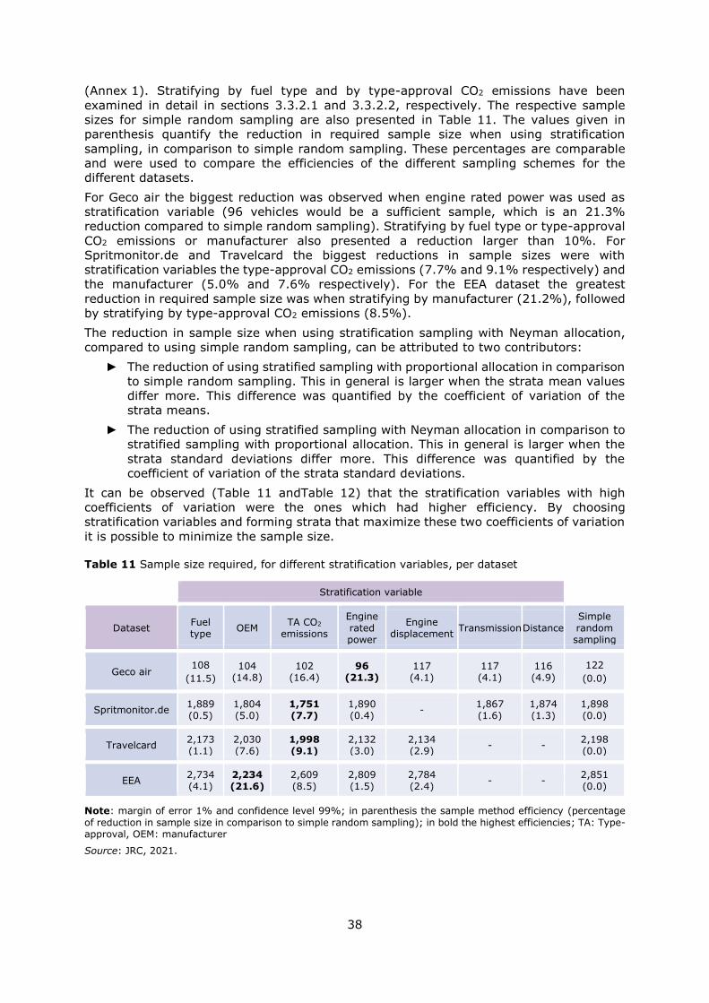
38

(Annex 1). Stratifying by fuel type and by type-approval CO2 emissions have been

examined in detail in sections 3.3.2.1 and 3.3.2.2, respectively. The respective sample

sizes for simple random sampling are also presented in Table 11. The values given in

parenthesis quantify the reduction in required sample size when using stratification

sampling, in comparison to simple random sampling. These percentages are comparable

and were used to compare the efficiencies of the different sampling schemes for the

different datasets.

For Geco air the biggest reduction was observed when engine rated power was used as

stratification variable (96 vehicles would be a sufficient sample, which is an 21.3%

reduction compared to simple random sampling). Stratifying by fuel type or type-approval

CO2 emissions or manufacturer also presented a reduction larger than 10%. For

Spritmonitor.de and Travelcard the biggest reductions in sample sizes were with

stratification variables the type-approval CO2 emissions (7.7% and 9.1% respectively) and

the manufacturer (5.0% and 7.6% respectively). For the EEA dataset the greatest

reduction in required sample size was when stratifying by manufacturer (21.2%), followed

by stratifying by type-approval CO2 emissions (8.5%).

The reduction in sample size when using stratification sampling with Neyman allocation,

compared to using simple random sampling, can be attributed to two contributors:

► The reduction of using stratified sampling with proportional allocation in comparison

to simple random sampling. This in general is larger when the strata mean values

differ more. This difference was quantified by the coefficient of variation of the

strata means.

► The reduction of using stratified sampling with Neyman allocation in comparison to

stratified sampling with proportional allocation. This in general is larger when the

strata standard deviations differ more. This difference was quantified by the

coefficient of variation of the strata standard deviations.

It can be observed (Table 11 andTable 12) that the stratification variables with high

coefficients of variation were the ones which had higher efficiency. By choosing

stratification variables and forming strata that maximize these two coefficients of variation

it is possible to minimize the sample size.

Table 11 Sample size required, for different stratification variables, per dataset

Stratification variable

Dataset Fuel type

OEM TA CO2

emissions

Engine

rated power

Engine displacement

Transmission Distance

Simple

random sampling

Geco air 108

(11.5)

104 (14.8)

102 (16.4)

96 (21.3)

117 (4.1)

117 (4.1)

116 (4.9)

122

(0.0)

Spritmonitor.de 1,889 (0.5)

1,804 (5.0)

1,751 (7.7)

1,890 (0.4)

- 1,867 (1.6)

1,874 (1.3)

1,898 (0.0)

Travelcard 2,173 (1.1)

2,030 (7.6)

1,998 (9.1)

2,132 (3.0)

2,134 (2.9)

- - 2,198 (0.0)

EEA 2,734 (4.1)

2,234 (21.6)

2,609 (8.5)

2,809 (1.5)

2,784 (2.4)

- - 2,851 (0.0)

Note: margin of error 1% and confidence level 99%; in parenthesis the sample method efficiency (percentage

of reduction in sample size in comparison to simple random sampling); in bold the highest efficiencies; TA: Type-approval, OEM: manufacturer

Source: JRC, 2021.

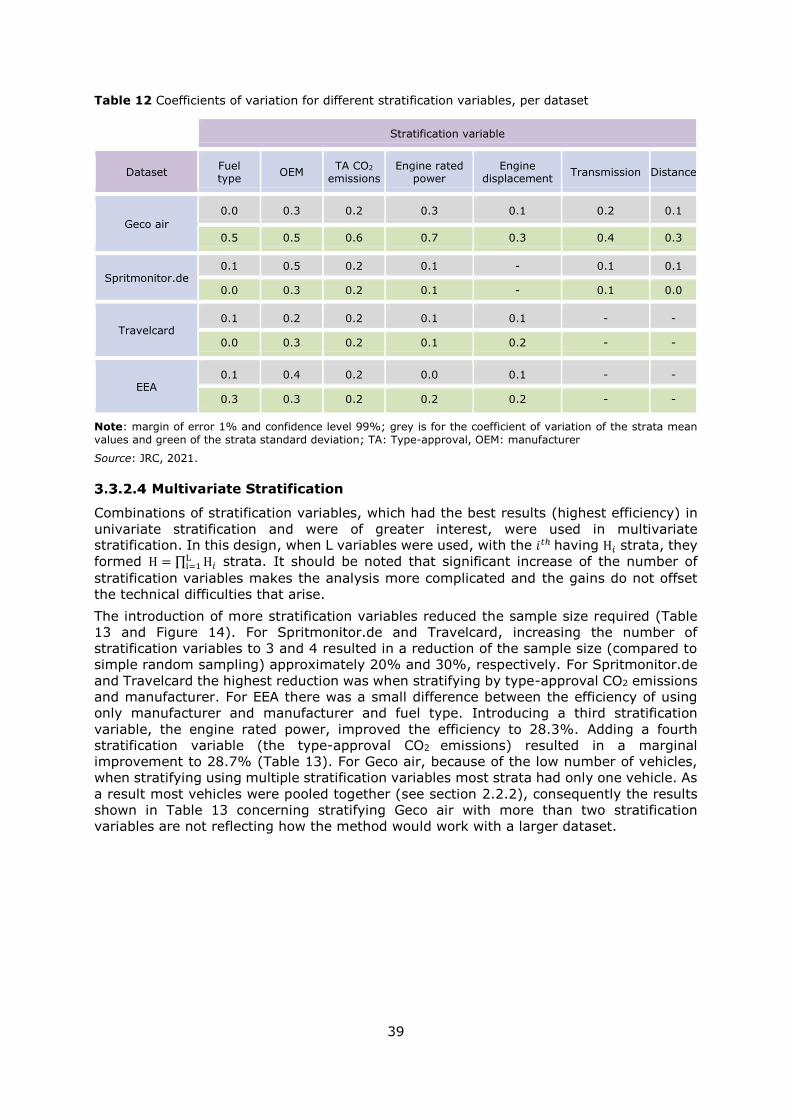
39

Table 12 Coefficients of variation for different stratification variables, per dataset


Dataset Fuel type

OEM TA CO2

emissions Engine rated

power Engine

displacement Transmission Distance

Geco air

0.0 0.3 0.2 0.3 0.1 0.2 0.1

0.5 0.5 0.6 0.7 0.3 0.4 0.3

Spritmonitor.de 0.1 0.5 0.2 0.1 - 0.1 0.1

0.0 0.3 0.2 0.1 - 0.1 0.0

Travelcard 0.1 0.2 0.2 0.1 0.1 - -

0.0 0.3 0.2 0.1 0.2 - -

EEA 0.1 0.4 0.2 0.0 0.1 - -

0.3 0.3 0.2 0.2 0.2 - -

Note: margin of error 1% and confidence level 99%; grey is for the coefficient of variation of the strata mean

values and green of the strata standard deviation; TA: Type-approval, OEM: manufacturer

Source: JRC, 2021.

Multivariate Stratification

Combinations of stratification variables, which had the best results (highest efficiency) in

univariate stratification and were of greater interest, were used in multivariate stratification. In this design, when L variables were used, with the 𝑖𝑡ℎ having H𝑖 strata, they

formed H = ∏ H𝑖Li=1 strata. It should be noted that significant increase of the number of

stratification variables makes the analysis more complicated and the gains do not offset

the technical difficulties that arise.

The introduction of more stratification variables reduced the sample size required (Table

13 and Figure 14). For Spritmonitor.de and Travelcard, increasing the number of

stratification variables to 3 and 4 resulted in a reduction of the sample size (compared to

simple random sampling) approximately 20% and 30%, respectively. For Spritmonitor.de

and Travelcard the highest reduction was when stratifying by type-approval CO2 emissions

and manufacturer. For EEA there was a small difference between the efficiency of using

only manufacturer and manufacturer and fuel type. Introducing a third stratification

variable, the engine rated power, improved the efficiency to 28.3%. Adding a fourth

stratification variable (the type-approval CO2 emissions) resulted in a marginal

improvement to 28.7% (Table 13). For Geco air, because of the low number of vehicles,

when stratifying using multiple stratification variables most strata had only one vehicle. As

a result most vehicles were pooled together (see section 2.2.2), consequently the results

shown in Table 13 concerning stratifying Geco air with more than two stratification

variables are not reflecting how the method would work with a larger dataset.

40

Table 13 Sample size required, for up to four stratification variables, per dataset

Stratification variable(s)

Dataset Fuel type

OEM TA CO2 Engine rated power

OEM &

Fuel type

OEM &

Fuel type&

Power

OEM &

Fuel type&

Power& TA CO2

Simple random sampling

Geco air 108

(11.5)

104

(14.8)

102

(16.4)

96

(21.3)

86

(29.5)

100

(18.0)

105

(13.9)

122

(0.0)

Spritmonitor.de 1,889

(0.5)

1,804

(5.0)

1,751

(7.7)

1,890

(0.4)

1,787

(5.8)

1,518 (20.0)

1,347 (29.0)

1,898

(0.0)

Travelcard 2,173

(1.1)

2,030

(7.6)

1,998

(9.1)

2,132

(3.0) 1,974 (10.2)

1,723 (21.6)

1,602 (27.1)

2,198

(0.0)

EEA 2,734

(4.1)

2,234

(21.6)

2,609

(8.5)

2,809

(1.5)

2210

(22.5)

2,045 (28.3)

2,032

(28.7)

2,851

(0.0)

Note: margin of error 1% and confidence level 99%; in parenthesis the sample method efficiency (percentage of reduction in sample size in comparison to simple random sampling); TA: Type-approval, OEM: manufacturer

Source: JRC, 2021.

Figure 14 Sample size required for different stratification variables, for EEA

Note: margin of error 1% and confidence level 99%; red dash line is sample size for simple random sampling; FT: Fuel type; TA: Type-approval; OEM: manufacturer; Power: Engine rated Power

Source: JRC, 2021.

Strata specific estimators

Regulation (EU) 2019/631 requires from the EC to monitor the fuel consumption gap of

each manufacturer. To accomplish this a precise estimator of the whole population average

fuel consumption gap is not enough. As described in section 2.2.2, in stratified sampling

unbiased estimators of each stratum mean are calculated and used to form an unbiased

estimator of the population mean. So far the main goal has been to find the minimum

sample size that ensures that the sample mean is a precise estimator of the population

mean. This section explores additional requirements so that the sample means of all/some

strata are precise estimators of their respective strata means. In this way sufficient vehicles

would be sampled from each stratum of interest to ensure that a separate analysis of these

strata can be performed. The higher the required precision, the higher the sample size per

stratum and consequently the total sample size. In the following analysis, for the sample

mean of the whole population, a margin of error of 1% with a confidence level of 99% was

used. Concerning the sample mean of each stratum, the conditions were less strict, a

margin of error of 2% with a confidence level of 90% was chosen.

41

In univariate stratification, when precise estimators are required for all strata, the higher

the number of strata, the bigger the increase in sample size compared to normal stratified

sampling. In multivariate stratification there are two options, either to demand precise

estimators for all strata or for only some of the stratification variables. E.g. if the

stratification variables are the manufacturer, the fuel type and the engine rated power,

there are 1044 = 58 ∗ 2 ∗ 9 strata, for EEA. If precise estimators for all 1044 strata are

needed, the total sample size would be 18,243 vehicles. However if only precise estimators

per manufacturer are required (58 strata) , then the sample size would be 3,094 vehicles.

The number of vehicles in the case of stratifying by manufacturer, fuel type, engine rated

power and requiring precise estimators only per manufacturer (3,094 vehicles) is of the

same order as the number of vehicles when stratifying by manufacturer and requiring

precise estimators for each manufacturer (3,068). Hence, only sample sizes for when

estimators for every stratum are required are discussed.

Figure 15 shows the sample size for the EEA dataset required to get precise estimators of

the mean fuel consumption gap, for different stratification schemes, when precise

estimators are required for all strata. For EEA, with four stratification variables

(manufacturer, fuel type, type-approval CO2 emissions and engine rated power) the

required sample size was almost 36 times larger (72,889 instead of 2,035 vehicles). When

only the mean fuel consumption gap of the whole population is required to be precise,

increasing the stratification variables leads to lower sample size (Table 14). On the other

hand when precise estimators for all strata are required, increasing the stratification

variables leads to a steep increase in sample size.

Table 14 Sample size, for up to four stratification variables, per dataset


Dataset Fuel type

OEM TA CO2 Engine rated power

OEM &

Fuel type

OEM &

Fuel type&

Power

OEM &

Fuel type&

Power& TA CO2

Simple random sampling

Geco air

108 104 102 96 86 100 120

122

108 114 107 98 104 116 105

Spritmonitor.de 1,889 1,804 1,751 1,890 1,787 1,518 1,347

1,898 1,889 1,945 1,751 1,890 2,131 3,428 4,293

Travelcard 2,173 2,030 1,998 2,132 1,974 1,723 1,602

2,198 2,173 2,345 1,998 2,132 2,538 4,784 7,224

EEA 2,734 2,234 2,609 2,809 2,210 2,045 2,032

2,851 2,734 3,051 2,609 2,809 3,767 18,238 72,865

Note: grey is for normal stratified sampling and green for stratifying sampling when the precise estimators are

required for all strata; margin of error 1% and confidence level 99%; TA: Type-approval, OEM: manufacturer

Source: JRC, 2021.

42

Figure 15 Sample size required for different stratification variables when strata specific estimators

are required for all strata

Note: EEA dataset, margin of error 1% and confidence level 99%; red dash line is sample size for simple random sampling; FT: Fuel type; TA: Type-approval; OEM: manufacturer; Power: Engine rated Power

Source: JRC, 2021.

3.3.3 Impact of non-sampling errors

The statistical approaches previously discussed and analysed are performed in such a way

that the sampling error is controlled and the sample size is minimized. The datasets used

are user-based with either self-reported data (Spritmonitor.de and Travelcard) or data

collected through GPS measurements and real-world CO2 emissions calculated by the

model (Geco air). The vehicles composing these three datasets are mostly from three

countries. As a result even though the datasets were found to represent, in respect to most

vehicle characteristics, the whole fleet of vehicles in a satisfactory manner, the whole

variability of the fleet, as concerns the vehicle characteristics, was not captured. To the

best of the authors’ knowledge there is no published research that explicitly quantifies the

differences in the fuel consumption gap from country to country across the EU. Additionally

the datasets suffer from self-selection bias, as in general users of these applications

(Spritmonitor.de and Geco air) are more environmental friendly and conservative with fuel

consumption. Users of Travelcard in general care less, since their companies provide them

the vehicles and pay the fuel costs. Additionally, it is difficult to quantify the reliability of

the values inserted by the users in Spritmonitor.de and Travelcard.

Most of these issues will not exist in the future as data will be extracted from the OBFCM

devices whose accuracy is set to ±5% compared to the fuel consumption reported in the

laboratory during WLTP type-approval test. In addition OBFCM accuracy is expected to

improve as the new technologies are introduced and the requirements and tests become

stricter. In this case it is of importance to quantify the measurement error of these devices

and to understand the impact that it will have on the sampling scheme. According to

previously published research (Pavlovic et al., 2021), in real-world conditions OBFCM

devices were found to have, in respect to measuring the fuel consumption in litres per

hundred kilometres (l/100km), a mean error/inaccuracy of 2.7% with a standard deviation

of 5.6%, compared to values calculated by Portable Emissions Measurement Systems

(PEMS). During laboratory (WLTP) tests the OBFCM devices had a mean error/inaccuracy

of 1.5% with a standard deviation of 4.5%.

Taking these into account, to get an indication of the impact of the OBFCM inaccuracies on

the sample size, a “noise” amounting to the respective on-road and type approval OBFCM

error was added to the real world and to the type approval fuel consumption of all vehicles.

It should be noted that the noise is not a cumulative addition to the fuel consumptions,

but a percentage dispersion. By doing this, the average fuel consumption gap of Geco air’s,

43

Spritmonitor.de’s, Travelcard’s and EEA’s vehicles increased by 1.9%, 1.7%, 1.8% and

1.9%, respectively. The standard deviation increased by 1.8%, 2.3%, 2.7% and 2.5%,

respectively (Table 15). Therefore for simple random sampling the required sample size to

have a margin of error of 1% and confidence level of 99% is increased by 1% (126->127),

17% (1898->2220), 27% (2198->2795) and 19% (2,851->3,267), respectively. For

stratified sampling the increases are expected to be of the same order. To get more precise

results an estimation/understanding of the OBFCM accuracy per stratum would be

necessary.

Table 15 Impact of non-sampling errors in simple random sampling, per dataset

Dataset

Standard deviation

increase

Sample size before

Sample size after

Sample size increase (%)

Geco air 1.8 122 123 1

Spritmonitor.de 2.3 1,898 2,222 17

Travelcard 2.7 2,198 2,798 27

EEA 2.5 2,851 3,580 26

Source: JRC, 2021.

3.3.4 Practical considerations for the implementation of quota sampling

Quota sampling is an alternative to choosing a representative sample when probability

sampling is not an option. If quota sampling is used, selecting as stratification variables

those that are correlated to the average fuel consumption gap gives some degree of control

over selection biases.

The relationship between the fuel consumption gap and other variables was examined

(section 3.2) and the efficiencies of using these variables in a univariate stratification

sampling design were compared (section 3.3.2.3). In conclusion, the vehicle manufacturer,

the type-approval CO2 emissions and the fuel type are the three variables that produce

better results. When using them the sample required to reach a pre-specified accuracy was

the smallest, equivalently with a pre-specified sample size a higher accuracy would be

reached when using them. These variables should be used if a quota sampling design is

implemented.

A study in Germany (Bluthner and Schroder, 2020) showed that approximately 10% of the

vehicles had performed the PTI by the first year of the vehicle’s registration. For the

selection of a representative sample, a feasible option could be to use vehicles from those

that perform the PTI test. However, care should be taken to understand whether the fuel

consumption gap is different for vehicles that do not go for an early PTI and if it varies

from one country to another. In such cases, suitable adaptions have to be made.

There are no specific formulas to calculate the sample size that would suffice for estimating

the fuel consumption gap with exhaustive precision. A general rule is to use at the least a

sample size as big as the one stratified sampling would require.

For each of the datasets a sample respecting the proportions of the EEA dataset (with

respect to the vehicle manufacturer, the type-approval CO2 emissions and the fuel type)

was chosen by selecting the first vehicles that satisfied these conditions. The sample sizes

were the same as the one required for stratification sampling with those three variables.

The sampling errors of the average fuel consumption were 2.9%, 2.2%, 3.4% and 2.4%

respectively for Geco air, Spritmonitor, Travelcard and EEA.

44

4 Conclusions

► The average fuel consumption gap of new vehicles registered in the EU can be

accurately estimated using a sample. Especially for the first level of analysis where

only the monitoring of the global emissions trend is required.

► The standard deviation of the fuel consumption gap of conventional pure internal

combustion and hybrid petrol and diesel LDVs in three user datasets was

consistently found to be approximately 20%.

► In simple random sampling the higher the variability of the fuel consumption gap

the more vehicles need to be sampled. For a population of 15 million vehicles, if the

standard deviation of the fuel consumption is 20%, a sample of fewer than 3,000

vehicles is required for estimating the average gap with a confidence level of 99%

and sampling error less than 1%. If the standard deviation of the fuel consumption

is 40%, approximately 10,500 vehicles are required.

► Stratified sampling can further reduce the required sample size. Of the different

allocation procedures, Neyman allocation produces the best results, but requires

the most a priori knowledge.

► For EEA dataset multivariate stratification with three stratification variables (vehicle

manufacturer, fuel type and engine rated power) required a sample size

approximately 28% less than simple random sampling. Adding a fourth stratification

variable (CO2 emissions) reduced the sample size by less than 1%.

► When precise estimators are demanded for each stratum the sample size increases.

As the number of stratification variables increases, the required sample size

escalates.

► Non-sampling errors are expected to enlarge the variability of the fuel consumption

gap by at least 2%-3% and consequently the sample size by ~20%.

► The quota sampling method is an alternative technique that can produce a

representative sample. The three stratification variables mentioned above and at

least the sample size of multivariate stratification is recommended in this case. A

quota sample was selected from each dataset. The sampling error in all four

datasets was found to be less than 3.5%.

45

References

Cochran, W.G. 1977. Sampling Techniques, 3rd Edition. 3rd edition. New York: John Wiley

& Sons

"Commission Implementing Regulation (EU) 2021/392 of 4 March 2021 on the Monitoring

and Reporting of Data Relating to CO2 Emissions from Passenger Cars and Light

Commercial Vehicles Pursuant to Regulation (EU) 2019/631 of the European Parliament

and of the Council and Repealing Commission Implementing Regulations (EU)

No 1014/2010, (EU) No 293/2012, (EU) 2017/1152 and (EU) 2017/1153"

Dornoff, J., Tietge, U., Mock, P. 2020. “On the Way to ‘Real-World’ CO2 Values: The

European Passenger Car Market in Its First Year after Introducing the WLTP”

Fontaras, G., Zacharof, N.G., Ciuffo, B. 2017. “Fuel Consumption and CO 2 Emissions from

Passenger Cars in Europe–Laboratory versus Real-World Emissions.” Progress in Energy

and Combustion Science 60: 97–131

Bluthner, F., Schroder, R. 2020. “Transfer of OBFCM Data to EC by FSD-CA.”

Ligterink, N.E., Smokers, R.T.M., Spreen, J., Mock, P., Tietge, U. 2016. “Supporting

Analysis on Real-World Light-Duty Vehicle CO2 Emissions.” TNO 2016

Lohr, S.L. 2019. Sampling: Design and Analysis: Design and Analysis. CRC Press

Ntziachristos, L., Mellios, G., Tsokolis, D., Keller, M., Hausberger, S., Ligterink, N.E., Dilara,

P. 2014. “In-Use vs. Type-Approval Fuel Consumption of Current Passenger Cars in

Europe.” Energy Policy 67 (April): 403–11. https://doi.org/10.1016/j.enpol.2013.12.013.

Pavlovic, J., Ciuffo, B., Fontaras, G., Valverde, V., Marotta, A. 2018. “How Much Difference

in Type-Approval CO2 Emissions from Passenger Cars in Europe Can Be Expected from

Changing to the New Test Procedure (NEDC vs. WLTP)?” Transportation Research Part A:

Policy and Practice 111 (May): 136–47. https://doi.org/10.1016/j.tra.2018.02.002.

Pavlovic, J., Fontaras, G., Broekaert, S., Ciuffo, B., Ktistakis, M.A., Grigoratos, T. 2021.

“How Accurately Can We Measure Vehicle Fuel Consumption in Real World Operation?”

Transportation Research Part D: Transport and Environment 90 (January): 102666.

https://doi.org/10.1016/j.trd.2020.102666.

Plötz, Patrick, Cornelius Moll, Georg Bieker, and Peter Mock. 2021. “From Lab-to-Road:

Real-World Fuel Consumption and CO 2 Emissions of Plug-in Hybrid Electric Vehicles.”

Environmental Research Letters 16 (5): 054078. https://doi.org/10.1088/1748-

9326/abef8c.

“Regulation 2017/1151 - Supplementing Regulation 715/2007 on Type-Approval of Motor

Vehicles with Respect to Emissions from Light Passenger and Commercial Vehicles (Euro 5

and Euro 6) and on Access to Vehicle Repair and Maintenance Information - EU Monitor.”

“Regulation (EC) No 443/2009 of the European Parliament and of the Council of 23 April

2009 Setting Emission Performance Standards for New Passenger Cars as Part of the

Community’s Integrated Approach to Reduce CO2 Emissions from Light-Duty Vehicles.”

“Regulation (EU) 2018/1832 of 5 November 2018 Amending Directive 2007/46/EC of the

European Parliament and of the Council, Commission Regulation (EC) No 692/2008 and

Commission Regulation (EU) 2017/1151 for the Purpose of Improving the Emission Type

Approval Tests and Procedures for Light Passenger and Commercial Vehicles, Including

Those for in-Service Conformity and Real-Driving Emissions and Introducing Devices for

Monitoring the Consumption of Fuel and Electric Energy”

“Regulation (EU) 2019/631 of the European Parliament and of the Council of 17 April 2019

Setting CO2 Emission Performance Standards for New Passenger Cars and for New Light

Commercial Vehicles, and Repealing Regulations (EC) No 443/2009 and (EU) No 510/2011”

“Regulation (EU) 2019/1242 of the European Parliament and of the Council of 20 June

2019 Setting CO2 Emission Performance Standards for New Heavy-Duty Vehicles and

46

Amending Regulations (EC) No 595/2009 and (EU) 2018/956 of the European Parliament

and of the Council and Council Directive 96/53/EC”

“Regulation (EU) No 333/2014 of the European Parliament and of the Council of 11 March

2014 Amending Regulation (EC) No 443/2009 to Define the Modalities for Reaching the

2020 Target to Reduce CO2 Emissions from New Passenger Cars.”

Tietge, U., Diaz, S., Mock, P., Bandivadekar, A., Dornoff, J., and Ligterink. N.E. “From

Laboratory to Road: A 2018 Update of Official and ‘Real-World’ Fuel Consumption and CO2

Values for Passenger Cars in Europe”

Tsiakmakis, S., Ciuffo, B., Fontaras, G., Anagnostopoulos, K., Arcidiacono, V., Praksova,

R., and Marotta. A. 2016. “Introducing a New Emissions Certification Procedure for

European Light-Duty Vehicles: Monte Carlo Simulation of the Potential Effect on Fleet

Carbon Dioxide Emissions.” Transp Res Rec J Transp Res Board 2572 (January): 66–77.

https://doi.org/10.3141/2572-08.

47

List of abbreviations and definitions

CO2 Carbon dioxide

EC European Commission

EEA European Environment Agency

EU European Union

HDVs Heavy-duty vehicles

ICCT International Council on Clean Transportation

JRC Joint Research Centre

LDVs Light-duty vehicles

NEDC New European Driving Cycle

PTI Periodic Technical Inspection

OBFCM On-Board Fuel and/or energy Consumption Monitor device

OTA Over-the Air-Transmission

WLTC Worldwide harmonized Light vehicles Test Cycle

WLTP Worldwide Harmonized Light Vehicles Test Procedure

48

List of figures

Figure 1 Depiction of relations between population, sampling frame and sample .......... 8

Figure 2 Stratifying sampling procedure .................................................................13

Figure 3 Representativeness of datasets per fuel type ..............................................21

Figure 4 Representativeness of datasets per manufacturer .......................................22

Figure 5 Representativeness of datasets per type-approval CO2 ................................22

Figure 6 Representativeness of datasets per engine rated power ...............................23

Figure 7 Representativeness of datasets per engine displacement .............................23

Figure 8 Histograms & statistics of fuel consumption gap, per dataset .......................25

Figure 9 Fuel consumption gap by fuel type and transmission type, per dataset. Red

triangles depict the mean values ............................................................................25

Figure 10 Fuel consumption gap by manufacturer, per dataset. Only manufacturers with

at least a share of 4% in one of the datasets are presented. Red triangles depict the

mean values ........................................................................................................26

Figure 11 Average fuel consumption gap in relation to type-approval CO2 emissions,

engine rated power, engine displacement and distance driven, per dataset ..................27

Figure 12 Sample size in relation to standard deviation, for simple random sampling to

achieve a confidence level of 99% and a margin of error of 1% for a population of 15

million vehicles .....................................................................................................28

Figure 13 Distributions of the sample mean of the fuel consumption gap, per dataset ..31

Figure 14 Sample size required for different stratification variables, for EEA ...............40

Figure 15 Sample size required for different stratification variables when strata specific

estimators are required for all strata .......................................................................42

49

List of tables

Table ES1 Statistics of the sampling error ............................................................... 5

Table 1 Available variables per dataset ...................................................................17

Table 2 Statistics of the fuel consumption gap, per dataset .......................................28

Table 3 Margin of error in relation to sample size and standard deviation, for simple

random sampling for a population of 15 million vehicles ............................................29

Table 4 Sample size required per dataset for different margins of error and confidence

levels, for simple random sampling .........................................................................30

Table 5 Accurate cases per dataset for different margins of error and confidence levels,

for simple random sampling ...................................................................................31

Table 6 Sampling error per dataset for margin of error 1% and confidence level 99%, for

simple random sampling ........................................................................................32

Table 7 Fuel consumption gap grouped by fuel type, per dataset ...............................34

Table 8 Sample sizes per dataset required for different margins of error and confidence

levels, with stratification variable the fuel type, per dataset .......................................35

Table 9 Statistics of the fuel consumption gap grouped by type-approval CO2 emissions,

per dataset ..........................................................................................................36

Table 10 Sample sizes required and sample allocation per dataset with stratification

variable the type-approval CO2 emissions ................................................................37

Table 11 Sample size required, for different stratification variables, per dataset ..........38

Table 12 Coefficients of variation for different stratification variables, per dataset .......39

Table 13 Sample size required, for up to four stratification variables, per dataset ........40

Table 14 Sample size, for up to four stratification variables, per dataset ....................41

Table 15 Impact of non-sampling errors in simple random sampling, per dataset ........43

Table 16 Statistics of the FC Gap grouped by manufacturer, per dataset ....................50

Table 17 Statistics of the FC Gap grouped by engine rated power, per dataset ............50

Table 18 Sample size required and sample allocation, with stratification variable the

engine rated power, for Neyman allocation, per dataset ............................................51

Table 19 Statistics of the FC Gap grouped by engine displacement, per dataset ..........51

Table 20 Sample size required and sample allocation, with stratification variable the

engine displacement, per dataset ...........................................................................52

Table 21 Statistics of the FC Gap grouped by distance, per dataset ...........................52

Table 22 Sample sizes required and sample allocation, with stratification variable the

distance, per dataset ............................................................................................53

Table 23 Statistics of the FC Gap grouped by transmission, per dataset .....................53

Table 24 Sample sizes required and sample allocation, with stratification variable the

transmission, per dataset ......................................................................................53

50

Annexes

Annex 1. Allocations and statistics

Table 16 Statistics of the FC Gap grouped by manufacturer, per dataset

OEM

Dataset



Minimum 2 17.9 6.0 2 -7.1 0.0 2 14.2 8.9 2 -17.8 9.5

Maximum 41 54.0 40.6 934 45.7 29.3 4,770 58.4 33.3 1,606,461 47.1 39.5

Mean 8.5 31.0 16.4 176 24.2 18.2 728.8 38.3 18.3 252,133.6 23.3 17.1

Standard deviation

9.9 9.2 8.7 212.1 10.8 5.0 1,101.9 8.9 4.8 376,145.5 10.2 5.3

Coefficient of variation

1.16 0.30 0.53 1.2 0.45 0.28 1.51 0.23 0.26 1.49 0.44 0.31

Source: JRC, 2021.

Table 17 Statistics of the FC Gap grouped by engine rated power, per dataset

Engine

rated power (kW)

Dataset



≤60 8 31.0 21.3 356 22 21.6 3,817 44.0 19.9 1767902 28.6 20.8

(60,70] 18 31.4 20.6 477 24.3 19.7 4,131 38.4 17.9 1690848 31.3 22.1

(70,80] 7 22.4 13.1 405 27.3 20.4 2,399 43.9 18.5 965798 31.7 20.6

(80,90] 32 28.9 11.0 1074 27.0 19.9 7,274 38.6 16.7 2580055 30.6 18.3

(90,100] 27 38.2 24.4 754 25.4 20.7 3,029 38.5 18.4 1306271 32.7 25.1

(100,110] 5 52.0 56.5 1455 24.6 18.4 3,529 35.5 21.1 1635021 30.9 18.0

(110,120] 12 30.0 12.1 256 23.5 19.8 548 36.2 17.9 315605 29.3 14.7

≥120 18 38.1 13.5 2441 25.6 19.5 2,237 35.2 21.5 2057343 29.5 19.8

NA - - - - - - - - - 2304904 30.2 22.5

Minimum 5 22.4 11.0 256 22.0 18.4 548 35.2 16.7 315605 28.6 14.7

Maximum 32 52.0 56.5 2441 27.3 21.6 7,274 44.0 21.5 2580055 32.7 25.1

Mean 15.9 34.0 21.6 902.2 25.0 20.0 3,370.5 38.8 19.0 1624860.8 30.5 20.2

Standard deviation

9.8 8.9 15.0 743.4 1.8 0.9 1,940.2 3.5 1.7 692534.1 1.3 3.0


0.61 0.26 0.69 0.82 0.07 0.05 0.58 0.09 0.09 0.43 0.04 0.15

Source: JRC, 2021.

51

Table 18 Sample size required and sample allocation, with stratification variable the engine rated

power, for Neyman allocation, per dataset

Engine rated power (kW)

Dataset


≤60 8 102 321 343

(60,70] 17 126 312 350

(70,80] 4 110 188 186

(80,90] 17 285 514 441

(90,100] 27 208 236 306

(100,110] 5 356 315 275

(110,120] 7 68 42 43

≥120 11 635 204 381

NA - - - 484

Total sample size 96 1,890 2,132 2,835


75.6 26.2 7.9 0.019

Note: Neyman allocation, margin of error 1% and confidence level 99%

Source: JRC, 2021.

Table 19 Statistics of the FC Gap grouped by engine displacement, per dataset

Engine Displacement (cc)

Dataset

Geco air Travelcard EEA

𝑁𝑖 𝑚𝑖 𝑠𝑑𝑖 𝑁𝑖 𝑚𝑖 𝑠𝑑𝑖 𝑁𝑖 𝑚𝑖 𝑠𝑑𝑖

≤1,000 18 34.9 22.9 7215 39.2 18.2 2726237 31.5 23.3

(1,000,1,200] 24 32.8 23.4 2671 38.7 17.2 1519122 30.6 17.9

(1,200,1,400] 4 29.6 22.7 1696 32.3 17.0 1920492 26.7 23.5

(1,400,1,600] 54 31.7 21.6 8973 40.6 17.5 4257143 31.2 20.7

(1,600,1,800] 0 - - 688 45.7 17.6 432167 33.7 11.7

(1,800,2,000] 21 37.8 13.4 4499 36.2 22.1 2748987 31.0 20.0

≥2,000 6 31.3 10.3 1222 43.5 24.0 1019503 29.0 15.4

NA - - - - - - 96 29.7 18.3

Minimum 4 29.6 10.3 688 32.3 17.0 96 26.7 11.7

Maximum 54 37.8 23.4 8973 45.7 24.0 4257143 33.7 23.5

Mean 21.2 33 19.1 3852 39.5 19.1 1827968.4 30.4 18.8

Standard deviation

18 2.9 5.7 3186.5 4.5 2.8 1394017.5 2.0 4.0


0.85 0.09 0.3 0.83 0.11 0.15 0.76 0.07 0.21

Source: JRC, 2021.

52

Table 20 Sample size required and sample allocation, with stratification variable the engine

displacement, per dataset

Engine displacement (cc) Dataset

Geco air Travelcard EEA

≤1,000 18 555 590

(1,000,1,200] 24 194 253

(1,200,1,400] 4 122 420

(1,400,1,600] 54 667 817

(1,600,1,800] NA 51 47

(1,800,2,000] 14 421 511

≥2,000 3 124 146

NA - - 0

Total sample size 117 2,134 2,784


92.1 7.9 0.019


Source: JRC, 2021.

Table 21 Statistics of the FC Gap grouped by distance, per dataset

Distance (k km)

Dataset

Geco air Spritmonitor.de

𝑁𝑖 𝑚𝑖 𝑠𝑑𝑖 𝑁𝑖 𝑚𝑖 𝑠𝑑𝑖

≤5 62 30.8 21.8 1,093 27.5 23.8

(5,10] 24 33.7 15.4 1,482 26.2 19.7

(10,15] 18 37.4 17.5 1,353 24.6 18.9

(15,20] 10 42.5 32.0 1,090 23.7 18.4

(20,25] 5 31.9 15.9 797 24.8 17.7

(25,30] 2 33.9 11.8 525 24.5 16.9

(30,35] 3 25.6 9.3 282 24.1 19

≥35 3 36.3 19.2 596 25.8 20.1

Minimum 2 25.6 9.3 282 23.7 16.9

Maximum 62 42.5 32.0 1,482 27.5 23.8

Mean 15.9 34.0 17.9 902.2 25.2 19.3

Standard deviation 20.3 5.0 6.9 421.4 1.3 2.1

Coefficient of variation 1.28 0.15 0.39 0.47 0.05 0.11

Source: JRC, 2021.

53

Table 22 Sample sizes required and sample allocation, with stratification variable the distance, per

dataset

Distance (k km)

Dataset


≤5 62 345

(5,10] 19 395

(10,15] 16 340

(15,20] 10 266

(20,25] 5 187

(25,30] 2 118

(30,35] 2 71

≥35 3 159

Total sample size 116 1,874


91.3 26.0


Source: JRC, 2021.

Table 23 Statistics of the FC Gap grouped by transmission, per dataset

Transmission

Dataset


𝑁𝑖 𝑚𝑖 𝑠𝑑𝑖 𝑁𝑖 𝑚𝑖 𝑠𝑑𝑖

Automatic 50 36.2 25.2 4,003 27.6 19.5

Manual 77 31.4 16.6 3,215 22.6 19.5

Minimum 50 31.4 16.6 3,215 22.6 19.5

Maximum 77 36.2 25.2 4,003 27.6 19.5

Mean 63.5 33.8 20.9 3,609 25.1 19.5

Standard deviation 19.1 3.4 6.1 557.2 3.6 0.0

Coefficient of variation 0.30 0.10 0.29 0.15 0.14 0.00

Source: JRC, 2021.

Table 24 Sample sizes required and sample allocation, with stratification variable the transmission,

per dataset

Transmission Dataset


Automatic 50 1,042

Manual 67 833

Total sample size 117 1,875


92.1 26.0


Source: JRC, 2021.

GETTING IN TOUCH WITH THE EU

In person

All over the European Union there are hundreds of Europe Direct information centres. You can find the address of the centre nearest you at: https://europa.eu/european-union/contact_en

On the phone or by email

Europe Direct is a service that answers your questions about the European Union. You can contact this service:

- by freephone: 00 800 6 7 8 9 10 11 (certain operators may charge for these calls),

- at the following standard number: +32 22999696, or

- by electronic mail via: https://europa.eu/european-union/contact_en

FINDING INFORMATION ABOUT THE EU

Online

Information about the European Union in all the official languages of the EU is available on the Europa website at: https://europa.eu/european-union/index_en

EU publications You can download or order free and priced EU publications from EU Bookshop at:

https://publications.europa.eu/en/publications. Multiple copies of free publications may be obtained by

contacting Europe Direct or your local information centre (see https://europa.eu/european-

union/contact_en).

https://europa.eu/european-union/contact_en


https://europa.eu/european-union/index_en

https://publications.europa.eu/en/publications



The European Commission’s science and knowledge service

Joint Research Centre

JRC Mission

As the science and knowledge service

of the European Commission, the Joint

Research Centre’s mission is to support

EU policies with independent evidence

throughout the whole policy cycle.

doi:10.2760/39369

ISBN 978-92-76-23986-4

KJ-N

A-3

0420-E

N-N

sampling approaches for road vehicle fuel consumption

Documents