Global Steady Prandtl Expansion Over a Moving Boundary

Sameer Iyer ∗

September 15, 2016

Abstract

In this three-part monograph, we prove that steady, incompressible Navier-Stokes

flows posed over the moving boundary, y = 0, can be decomposed into Euler and

Prandtl flows in the inviscid limit globally in [1,∞)× [0,∞), assuming a sufficiently

small velocity mismatch. Sharp decay rates and self-similar asymptotics are extracted

for both Prandtl and Eulerian layers. We then develop a functional framework to

capture precise decay rates of the remainders, and prove the corresponding embedding

theorems by establishing weighted estimates for their higher order tangential derivatives.

These tools are then used in conjunction with a third order energy analysis, which in

particular enables us to control the nonlinearity vuy globally.

Contents

1 Introduction 3

Chapter I: Construction of Profiles 14

2 Overview of Results 14

3 Asymptotics of Prandtl Layer, u0p: 16

3.1 Existence of Front Profile . . . . . . . . . . . . . . . . . . . . . . . . . . . . 17

3.2 Zeroeth Prandtl Layer, u0p . . . . . . . . . . . . . . . . . . . . . . . . . . . . 21

4 Euler-1 Layer 30

4.1 Derivation of Equations . . . . . . . . . . . . . . . . . . . . . . . . . . . . . 30

4.2 Uniform Decay Estimates . . . . . . . . . . . . . . . . . . . . . . . . . . . . 31

∗sameer_iyer@brown.edu. Division of Applied Mathematics, Brown University, 182 George Street,

Providence, RI 02912, USA. Partially supported by NSF grant 1209437.

1

arX

iv:1

609.

0539

7v1

[m

ath.

AP]

17

Sep

2016

5 Prandtl Layer 1 39

5.1 Derivation of Linearized Prandtl Equations: . . . . . . . . . . . . . . . . . . 39

5.2 Global in x Existence and Decay: . . . . . . . . . . . . . . . . . . . . . . . . 43

6 Intermediate Layers 52

6.1 Construction of Euler Layer, [uie, vie] . . . . . . . . . . . . . . . . . . . . . . 53

6.2 Construction of Prandtl Layer, [uip, vip] . . . . . . . . . . . . . . . . . . . . . 56

6.3 Final Prandtl Layer . . . . . . . . . . . . . . . . . . . . . . . . . . . . . . . 70

Chapter II: a-Priori Estimates for Remainder 80

7 Overview of Results 80

8 The Function Space Z 82

8.1 Elliptic Estimates and the Spaces Yi . . . . . . . . . . . . . . . . . . . . . . 85

8.2 Embedding Theorems for the Space Z . . . . . . . . . . . . . . . . . . . . . 94

8.3 Function Space, Z(ΩN ) . . . . . . . . . . . . . . . . . . . . . . . . . . . . . 99

9 Navier-Stokes Remainders: Energy Estimates 100

9.1 Energy Estimates . . . . . . . . . . . . . . . . . . . . . . . . . . . . . . . . . 101

9.2 Positivity Estimate . . . . . . . . . . . . . . . . . . . . . . . . . . . . . . . . 107

9.3 Second Order Bounds . . . . . . . . . . . . . . . . . . . . . . . . . . . . . . 111

9.4 Third Order Bounds . . . . . . . . . . . . . . . . . . . . . . . . . . . . . . . 130

10 Nonlinear Analysis 143

10.1 a-priori Estimate of Nonlinearities . . . . . . . . . . . . . . . . . . . . . . . 143

Chapter III: Existence and Uniqueness 154

11 Overview of Results 154

12 Step 1: Invertibility of Weighted Stokes Operator, Sα 156

13 Step 2: Compact Perturbations, Sαψ + T [ψ] 162

14 Step 3: Nonlinear Existence of Auxiliary Systems 180

2

15 Step 4: Nonlinear Existence 184

16 Step 5: Uniqueness 186

1 Introduction

We consider the steady, incompressible Navier-Stokes equations in two dimensions:

UNSUNSX + V NSUNSY + PNSX = ε∆UNS , (1.1)

UNSV NSX + V NSV NS

Y + PNSY = ε∆V NS , (1.2)

UNSX + V NSY = 0, (1.3)

in the domain,

Ω = [1,∞)× R+. (1.4)

The boundary Y = 0 is moving with velocity ub > 0. The no-slip boundary conditions are

placed on this portion of the boundary:

UNS(X, 0) = ub = 1− δ, V NS(X, 0) = 0. (1.5)

The boundary conditions at X = 1 will be prescribed explicitly in the text. We take X = 1

for convenience (this enables us to replace weights of (1 + x)k with xk). Throughout this

paper, we assume that prescribed Euler flow is the shear flow:

(UE , V E) = (1, 0). (1.6)

We are interested in the limit as ε → 0. Formally, one expects that the solutions to

Navier-Stokes equations in (1.1) - (1.3) converges to the Euler shear flow in (1.6). This does

not happen, however, due to the mismatch at the boundary Y = 0, between the no-slip

condition enforced for Navier-Stokes, (1.5), and UE(X,Y = 0) = 1.

To account for the mismatch at the boundary, Prandtl in 1904 proposed a thin fluid

boundary layer which connects the velocity of ub to the Euler velocity of 1. The Prandtl

hypothesis is that the Navier-Stokes solutions can be decomposed, up to leading order in ε,

as the sum of the prescribed Euler flow and a boundary layer, the latter of which corrects

the disparity at the boundary between Euler and Navier-Stokes:

UNS = 1 + u0p + h.o.t(ε), V NS = 0 +

√εv0p +√εv1e + h.o.t(ε).1 (1.7)

1Here, “h.o.t” is an acronym for “higher order terms.”

3

The contribution of this paper is to validate the boundary layer theory, equations (1.7),

in the domain Ω, which in particular implies that the tangential variable can be taken in

[1,∞) if the mismatch is sufficiently small :

UE − UNS |Y=0 = 1− ub = 1− (1− δ) = δ << 1. (1.8)

Boundary Layer Expansion

We will work with scaled, boundary layer variables:

x = X, y =Y√ε. (1.9)

The scaled Navier-Stokes unknowns are then given by:

U ε(x, y) = UNS(X,Y ), V ε(x, y) =V NS(X,Y )√

ε, P ε(x, y) = PNS(X,Y ). (1.10)

These unknowns satisfy the following system:

U εU εx + V εU εy + P εx = U εyy + εU εxx, (1.11)

U εV εx + V εV ε

y +P εyε

= V εyy + εV ε

xx, (1.12)

U εx + V εy = 0. (1.13)

Note that the steady Prandtl system is obtained by considering the leading order in ε of

the above system (1.11) - (1.13). We start with the following asymptotic expansion:

U ε(x, y) = 1 + u0p +

n∑i=1

εi2uie + ε

i2uip + ε

n2

+γu(x, y), (1.14)

V ε(x, y) =

n−1∑i=0

εi2 vip + ε

i2 vi+1e + ε

n2 vnp + ε

n2

+γv(x, y), (1.15)

P ε(x, y) =

n∑i=1

εi2P ie + ε

i2P ip + εiP i,ae + ε

i+12 P i,ap + ε

n2

+γP (x, y). (1.16)

Here, γ ∈ [0, 14). We will use the word “profiles” to refer to the terms which appear in

the expansions (1.14) - (1.15), excluding the remainders, [u, v, P ]. All of the profiles with

subscript-e are functions of Eulerian variables, (x, Y ), whereas all terms with subscript-p

are functions of boundary layer variables, (x, y). Here, [uip, vip] are boundary layers to be

4

constructed. The number of intermediate layers, n, is dependent on universal constants.

The pressures P ie , Pip are the pressures associated with the i′th Euler and Prandtl layers,

respectively. We will show that P ip = 0, that is the leading-order pressure in the boundary

layers is zero. The pressures P i,aP , P 1,ae are auxiliary pressures, which are higher-order,

whose purpose is to capitalize on the gradient structure of our problem (see 6.33). After

these layers are constructed, the Navier-Stokes remainders [u, v, P ] are then constructed.

Let us now designate names for the partial expansions:

u(i)s := 1 +

i−1∑j=0

εj2ujp +

i∑j=1

εj2uje, u(i)

s := u(i)s + ε

i2uip = 1 +

i∑j=0

εj2ujp +

i∑j=1

εj2uje (1.17)

v(i)s :=

i−1∑j=0

εj2 vjp +

i∑j=1

εj2− 1

2 vje, v(i)s := v(i)

s + εi2 vip =

i∑j=0

εj2 vjp +

i∑j=1

εj2− 1

2 vje, (1.18)

For the Pressure expansion:

P (i)s :=

i−1∑j=1

εj2P jp +

i−1∑j=1

εj+12 P j,ap +

i∑j=1

εj2P je +

i∑j=1

εjP j,ae . (1.19)

P (i)s :=

i∑j=1

εj2P jp +

i∑j=1

εj2P je +

i∑j=1

εjP j,ae +

i∑j=1

εj+12 P j,ap . (1.20)

We insert the expansions (1.14) - (1.16) into (1.11) - (1.13) and collect a heirarchy of

equations in powers of ε. Doing so yields the linearized Prandtl-equations:

(1 + u0p)u

ipx + u(i)

sxuip + v(i)

s uipy + u0py

(vip − vip(x, 0)

)+ P ipx = uipyy + f (i), (1.21)

uip(x, 0) = −uie(x, 0), limy→∞

uip(x, y) = 0, uip(1, y) = Ui(y). (1.22)

and the Euler equations:

uiex + P iex = 0, viex + P ieY = 0, uiex + vieY = 0. (1.23)

The forcing term f (i) will be defined precisely in (6.47). These equations are derived

rigorously in the analysis leading up to equations (4.5), (5.21), (6.19), and (6.48).

Boundary Data:

The no-slip boundary condition at the boundary y = 0 is the most important, and must

be enforced at each order in ε, which gives:

u0p(x, 0) = −δ, uie(x, 0) + uip(x, 0) = 0 for i ≥ 1, u(x, 0) = 0, (1.24)

5

vi−1p (x, 0) + vie(x, 0) = 0 for i ≥ 1, vnp (x, 0) = 0, v(x, 0) = 0. (1.25)

The in-flow (x = 1) boundary conditions for the leading order boundary layer, u0p, is:

u0p(1, y) = U0(y), U0(0) = −δ, lim

y→∞U0(y) = 0. (1.26)

We assume the rapid decay of the profile:

||〈y〉m∂jyU0(y)||L∞ ≤ C(m, j), for any m, j ≥ 0. (1.27)

We will in addition assume the following smallness condition:

||〈y〉m∂jyU0(y)||L∞ ≤ O(δ; j,m) for any m ≥ 0, j = 0, 1, 2. (1.28)

The in-flow (x = 1) boundary conditions for the boundary-layer profiles are:

uip(1, y) = Ui(y), u(1, y) = 0, v(1, y) = 0, for 1 ≤ i ≤ n− 1. (1.29)

Here, Ui(y), for i ≤ 1 ≤ n− 1, will be prescribed to be rapidly decaying in y, so:

||〈y〉muip(1, y)||L∞ = ||〈y〉mUi(y)||L∞ ≤ C(i,m) for 1 ≤ i ≤ n− 1. (1.30)

For the final Prandtl layer, unp , which occurs at order εn2 , the in-flow data is determined

through the analysis and is not explicitly prescribed. This is due to retaining that [unp , vnp ]

are divergence free, while cutting off vnp for large values of y. The reader is invited to turn

to equation (6.142) and corresponding discussion for details regarding this matter. We

will enforce ||〈y〉mUn(y)||L∞ ≤ C(m). However Un is an auxiliary in-flow, which is used to

construct [unp , vnp ]. That is: unp (1, y) 6= Un(y), and the in-flow velocity, unp (1, y), is given by

an implicit, bounded profile which decays as y →∞. We will need several compatibility

conditions on the in-flow data for the Prandtl layers. The first of these is:

U0(0) = −δ, ∂yyU0(y) = 0, Ui(0) = −uie(1, 0). (1.31)

However, we shall also need higher-order compatibility conditions on the Ui(y) at y = 0,

(see for instance Remarks 3.6, 5.11) which we refrain from depicting explicitly here. Finally,

the boundary conditions of the boundary-layer profiles as y →∞ are:

limy→∞

[uip(x), vip(x)] = limy→∞

[u(x), v(x)] = 0 for all x ≥ 1, and all 0 ≤ i ≤ n. (1.32)

6

These boundary conditions are known as the “matching condition”, and physically corre-

spond to the Navier-Stokes flow matching the outer Euler flow away from the boundary,

y = 0. According to our construction, we will have rapid matching up to order εn−12 :

limy→∞

[〈y〉Nuip(x), 〈y〉Nvip(x)] = 0 for all x ≥ 1, for 1 ≤ i ≤ n− 1. (1.33)

At the highest-order in ε, we enforce the matching condition:

limy→∞

εn2 [unp (x, y), vnp (x, y)] = lim

y→∞εn2

+γ [u(x, y), v(x, y)] = 0 for all x ≥ 1. (1.34)

Let us now turn to the Euler flows. At leading order, we have the prescription: [u0e, v

0e ] =

[1, 0]. The higher-order Euler flows will be described starting in Section 4 and Subsection

6.1. The higher-order Euler flows are obtained as suitable Poisson extensions of the Y = 0

boundary data, vi−1p (x, 0) (see (1.24)), which depend on the constructed Prandtl layers. For

these higher-order Euler flows, we do not prescribe the in-flow data, uie(1, Y ). Rather, the

in-flow conditions are obtained through the analysis, so we state:

Eulerian In-Flow =1 +n∑i=1

εi2uie(1, ·). (1.35)

Main Result:

In order to state our main result, we need to introduce the norm Z in which we control the

remainder solutions, [u, v]:

Definition 1.1. The norm Z is defined through:

||u, v||Z :=||u, v||X1∩X2∩X3 + εN2 ||u, v||Y2 + εN3 ||u, v||Y3 + εN4 ||ux14 ,√εvx

12 ||L∞

+ εN5 supx≥20||√εvxx

32 , uxx

54 ||L∞ + εN6 sup

x≥20||uyx

12 ||L2

y

+ εN7

[ ∫ ∞20

x4||√εvxx||2L∞y dx

] 12. (1.36)

Here, Ni, are large numbers which will be specified in (8.103) - (8.105). They depend only

on universal constants. The parameter n from (1.14) - (1.15) will be taken much larger

than any of the Ni. The norms || · ||Xi are energy norms defined in (8.3) - (8.5). The norms

|| · ||Yi are elliptic norms defined in (8.6) - (8.7). For the purposes of stating the main result,

7

we can refrain from being too specific with regards to the definitions of these norms. The

essential point that we will record concerns the uniform component:

εN4 ||ux14 ,√εvx

12 ||L∞ ≤ ||u, v||Z , (1.37)

The main result of this paper is:

Theorem 1.2. Suppose the the outer Euler flow is prescribed with u0e = 1. Suppose the

boundary and in-flow data are specified satisfying the conditions outlined in (1.24) - (1.34).

Then there exists an n depending on only universal constants such that the asymptotic

expansions in (1.14) - (1.16) are valid globally on the domain Ω, for 0 ≤ γ < 14 , so long as

the mismatch between the Eulerian boundary trace and the motion of the boundary, δ, and

the viscosity, ε, are taken sufficiently small relative to universal constants, and ε << δ. The

remainders, [u, v], in the expansions (1.14) - (1.15) are uniquely determined in the space Z:

||u, v||Z . ε14−γ−κ, (1.38)

where κ is any fixed constant such that γ + κ < 14 .

Because n2 is large relative to N4 in (1.37), we immediately find:

Corollary 1.3 (Inviscid L∞ Convergence). Under the hypothesis of Theorem 1.2, there

exists a unique Navier-Stokes solution [UNS , V NS , PNS ] on Ω such that:

sup(X,Y )∈Ω

∣∣∣UNS(X,Y )− 1− u0p(X, y)

∣∣∣X 14 . ε

12 , (1.39)

sup(X,Y )∈Ω

∣∣∣V NS(X,Y )−√εv0p(X, y)−

√εv1e(X,Y )

∣∣∣X 12 . ε. (1.40)

Existing Literature:

Let us first discuss the issue of establishing wellposedness of the Prandtl equation, which

becomes an issue in the unsteady setting (in contrast to the steady setting of the present

paper). This program was initiated in the classic works [OS99], [Ol67], in which, under

the monotonicity assumption U εy(t = 0) > 0, globally regular solutions are constructed

on the [0, L] × R+, where L is sufficiently small, and local solutions are constructed for

arbitrary, but finite L. This was extended in [XZ04], in which global weak solutions were

constructed for arbitrary L, under both monotonicity and favorable outer-Euler pressure

(∂xPE(t, x) ≤ 0 for t ≥ 0) assumptions.

8

From a physical standpoint, the monotonicity and favorable pressure assumptions men-

tioned above are stabilizing and in particular prevent boundary layer separation. This

phenomena was known to Prandtl, see Figure 2 in [Pr1905]. More recently, it was announced

in [DM15] that a proof of boundary layer separation in the steady setting has been obtained.

The main tool used both in [Ol67] and [XZ04] is the Crocco transform. Still under mono-

tonicity hypothesis, local wellposedness was obtained in [AWXY15] and [MW15], neither

works using the Crocco transform. [AWXY15] use energy methods coupled with a Nash-

Moser iteration, and [MW15] use energy methods applied to a good unknown which enjoys

crucial cancellation properties. Generalizing to multiple monotonicity regions, [KMVW14]

have shown the Prandtl equation is locally well-posed, if an analyticity assumption is made

on the complement of the monotonicity regions.

Indeed, when the assumption of monotonicity is removed, the wellposedness results are

largely in the analytic or Gevrey setting. The reader should consult [SC98] - [SC98], [KV13],

[LCS03], [IV16], and [GVM13] for some results in this direction. In the Sobolev setting

without monotonicity, the equations are linearly and nonlinearly ill-posed (see [GVD10]

and [GVN12]). A finite-time blowup result was obtained in [EE97] when the outer Euler

flow is taken to be zero, in [KVW15] for a particular, periodic outer Euler flow, and in

[HH03] for both the inviscid and viscous Prandtl equations. The above discussion is not

comprehensive: we refer the reader to the review articles, [E00], [GJT16] and references

therein for a more thorough review of the wellposedness theory.

The question with which we are concerned is the validity of the asymptotic expansion

(1.14) - (1.16) in the inviscid limit. Let us first discuss unsteady flows. Local-in-time

convergence is established in [SC98], [SC98] in the analyticity framework, in [GVMM16]

in the Gevrey setting, and in [Mae14] when the initial vorticity distribution is supported

away from the boundary. The reader should see also [As91], [MT08] for related results.

Despite the boundary layer classically having thickness√ε, an interesting criteria was given

in [Ka84] which points to phenomena occurring in a sub-layer of size ε. There are also

several linear and nonlinear instability results (for instance, [Gre00], [GGN15a], [GGN15b],

[GGN15c], [GN11]) which show the invalidity of Prandtl’s expansion generically in Sobolev

spaces in the unsteady setting.

For steady flows, there are very few validity results. [GN14] is the first result in this

direction, establishing validity of the boundary layer expansion for steady state flows in

a rectangular domain over a moving boundary. Geometric effects of the boundary were

subsequently considered in [Iy15]. The crucial idea in [GN14] was the use of a positivity

9

estimate, which is coupled with energy estimates and elliptic estimates. Both of these

results are local in the tangential variable. In the present work, we prove validity of the

boundary layer expansion globally in the tangential variable, x, in the setting of small data.

One preliminary piece of our analysis is to obtain the asymptotics of the Prandtl layer, u0p.

This has nontrivial dynamics due to the mismatched boundary conditions, u0p(y = 0) = −δ,

while limy→∞ u0p(y) = 0. These asymptotics were first studied in [Ser66, pg. 493, Inequality

5] using maximum principle techniques and are valid for large data. The result in [Ser66]

gives that the difference between u0p and a Gaussian“front” solution to the heat equation

(call it w) is o(1) in x, uniformly in y. Under the hypothesis of small data, we sharpen these

asymptotics in the following sense: first, w is shown to belong to a higher-order Sobolev

space Hk(m), where this weight is in the self-similar variable z = y√x. Second, we obtain

rates of decay of w in x in various norms.

We now detail the main difficulties and ideas behind our analysis.

Sharp Decay of Profiles (Chapter I):

The key issue that we must capture in our analysis is the decay as x → ∞ of various

quantities. More specifically, a central difficulty is to control contributions from the

nonlinearity V εU εy . Let us now introduce the equations for the remainders, [u, v, P ]:

−∆εu+ Su + Px = f, −∆εv + Sv +Pyε

= g, ux + vy = 0. (1.41)

Here, the terms Su, Sv contain the linearizations of [u, v] around the previously constructed

profiles, [u(n)s , v

(n)s ]. These terms, together with f, g are specifically defined in (7.5) - (7.6).

To organize this discussion, let us record the heuristic:

Difficult Contributions from V εU εy = u(n)sy v + v(n)

s uy + εn2

+γvuy. (1.42)

First, let us discuss u(n)sy v from (1.42), which will motivate the crucial decay rates appearing

in (1.48). Applying the scaled multiplier of (u, εv) to the system (1.41) requires controlling

the large convective term,∫ ∫

u0pyuv. We do not have the ability to create a derivative

through the Poincare inequality, and so we trade factors of x and y in the following manner:∣∣∣ ∫ ∫ u0pyuv

∣∣∣ ≤ ||u0pyy

2x−12 ||2L∞ ||

u

y||L2 ||

vx12

y||L2 ≤ O(δ)||uy||L2 ||vyx

12 ||L2 . (1.43)

The first crucial observation we make is the identification of a self-similar front, φ∗(y√x),

which bridges the boundary conditions: u0p(x, 0) = −δ, u0

p(x,∞) = 0. Then, temporarily

identifying u0p ≈ φ∗(

y√x), (1.43) will be satisfied:

10

Requirement 1.4 (Self-Similarity of Prandtl profiles).

||y2x−12u0

py||L∞ = ||y2x−1φ′∗

( y√x

)||L∞ = ||z2φ′∗(z)||L∞ ≤ O(δ). (1.44)

Summarizing the energy estimate that we obtain:

||uy||2L2 ≤ O(δ)||√εvx, vyx

12 ||2L2 + Forcing Terms. (1.45)

Above, the key point is the loss of weight, x12 . The next ingredient is recovering this weight

in the Positivity estimate, (see Proposition 9.4), which is summarized:

||√εvx, vyx

12 ||2L2 . ||uy||2L2 + Forcing Terms. (1.46)

In order to prove (1.46), we must apply the weighted multilplier vyx. Referring to the final

two terms in (1.42), this gives (temporarily ignoring factors of ε):∣∣∣ ∫ ∫ v(n)s uy · vyx

∣∣∣+∣∣∣ ∫ ∫ vuy · vyx

∣∣∣ ≤ ||v(n)s , vx

12 ||L∞ ||uy||L2 ||vyx

12 ||L2 . (1.47)

The latter two L2 quantities are controlled by the left-hand sides of (1.46) - (1.47). From

this, we obtain the requirements:

Requirement 1.5 (Uniform Decay).

v(n)s + v ∼ x−

12 , as x→∞. (1.48)

We emphasize that this requirement is inflexible, and we cannot sacrifice even a logarithmic

factor of x here. The main contribution of Chapter I is the construction of profiles

uip, vip, u

ie, v

ie which satisfy the requirement of v

(n)s in (1.48). The most difficult task is to

obtain the estimate (1.48) for the Eulerian profiles, v1e , as these are solutions to elliptic

boundary value problems in which the boundary condition exhibits exactly the required

decay rate, |v1e(x, 0)| ≤ x−

12 . We refer the reader to the crucial Proposition 4.2 in which

we introduce novel techniques centered around the explicit integral representation of v1e ,

enabling us to prove the required decay, |v1e | . x−

12 .

Note that we construct the expansions, (1.14) - (1.16) for any n ∈ N, which is required as

discussed in the paragraph following (1.52). Our ability to do this relies on the Cauchy-

Riemann structure of the Eulerian profiles, which we use in Lemma 6.33.

11

The Norm Z (Chapter II):

Let us now turn to the v term in Requirement (1.48): the main contribution of Chapter II

is to prove the required decay estimate |v| . x−12 by using the crucial norm Z (see Lemmas

8.16, 8.19). The challenge is to extract this precise uniform decay information from the

energy norms that are controlled. Bearing in mind the inflexibility of (1.48), obtaining the

decay for v using the norms Xi is an extremely delicate matter, in which key quantities must

overcome the critical Hardy inequality. To see this, we first use the H1y (R+) → L∞y (R+)

Sobolev embedding (ignoring factors of ε):

supx≥1||vx

12 ||L∞y ≤ sup

x≥1||v||

12

L2y· supx≥1||vyx||

12

L2y. (1.49)

For the first quantity on the right-hand side above, we write:

∂x

∫v2 dy =

∫2vvx dy. (1.50)

Recall now the quantities, ||uy,√εvxx

12 , vyx

12 ||2L2

xy, which are controlled on the left-hand

sides (1.45), (1.46) and constitute the energy norm X1. The right-hand side above fails to

be x-integrable, precisely because of criticality of Hardy’s inequality with power x−12 in L2:

|∫ ∫

vvx dy dx| ≤ ||vx−12 ||L2

xy||vxx

12 ||L2

xy@@≤||vxx12 ||2L2

xy. (1.51)

To avert this, we move to higher-order derivatives, which invokes the full strength of the

norm Z. Indeed, suppose we knew vx ∼ x−32 , then coupled with the boundary condition

v → 0 as x → ∞, this would immediately imply v ∼ x−12 . Establishing the decay rate,

||vx||L∞y ≤ x−32 , then becomes the goal, which requires us to go to third-order energy

estimates (thus explaining the presence of X1, X2, X3 in the norm Z). Our main uniform

estimates, given in Lemmas 8.16, 8.19 are given by the following sequence:

||vx12 ||L∞xy . ||vxx

32 ||L∞xy . sup

x≥1||vxx||

12

L2y· supx≥1||vxyx2||

12

L2y. ||u, v||X1∩X2∩X3 . (1.52)

The key point is that the quantities ||vxx||L2y

and ||vxyx2||L2y

appearing above do not face

issues of Hardy-criticality present in (1.51), which can be seen in Lemma 8.16.

Applying ∂kx to the system creates singularities near the corner at (1, 0). To handle this

we cutoff near the boundary, x = 1, when performing higher order energy estimates. Cutoff

functions interact poorly with nonlinearities, and so we need to supplement energy estimates

12

with elliptic estimates which retain additional control of [u, v] near x = 1 (though not

all the way up to the boundary, x = 1). These are characterized by the norms || · ||Yi in

(1.36). These Yi norms are controlled by invoking the elliptic theory, which in turn requires

sacrificing factors of ε. For this, we require a high power of εn to accompany nonlinear

terms, which in turn requires us to go to high order expansions in (1.14) - (1.16).

Existence and Uniqueness (Chapter III):

Upon proving our main a-priori estimate, Theorem 7.1, we prove existence and uniqueness

of a solution in Z. As in (1.43), applying the multiplier u produces the nonlinearity vuy · u,

which is a perfect derivative and therefore vanishes. This cancellation property is destroyed

upon taking differences, and so we cannot rely on a standard application of the contraction

mapping theorem. A sequence of auxiliary, approximate systems are then carefully designed

to produce enough compactness enabling us to show existence of a solution in the space Z.

The uniqueness in Z is a more delicate matter, again due to a lack of the perfect derivative

structure. For this, we take the difference of two solutions in Z and repeat the energy

analysis with weaker weights. The reader is referred to Lemma 16.1, in which the weights

must be selected carefully in a small interval below those weights appearing in the energy

analysis, for instance in (1.45), (1.46). These methods are carried out in Chapter III.

Notation and Important Parameters

There are three important parameters in this paper: ε, δ, and n (see (1.14) - (1.16)). The

notation A . B means A ≤ CB, where C is some constant which is independent of small

δ, ε, and large n. Constants denoted by O(δ) or O(ε) satisfy O(δ),O(ε) → 0 as δ, ε → 0,

respectively. Given any parameter, say p, constants denoted by C(p) mean those constants

which depend (perhaps poorly) on large values of p. Given two parameters, δ and σ, for

instance, we will write O(δ;σ) to denote a constant which depends on σ and δ, but such

that for fixed σ, δ can be made small to make the constant small, for instance δ × σ. We

define ||f ||pLpy

:=∫f(x, y)pdy. When unspecified, || · ||Lp means the Lp norm of two-variables.

We define here the differential operators:

∆εu := (∂xx + ε∂yy)u for any profile u; ∆[uie, vie] := (∂xx + ∂Y Y )[uie, v

ie]. (1.53)

The variable z will denote a self-similar variable, so typically z = y√x

or z = η√x. Finally,

the word “profiles” refers to terms in the expansion (1.14) - (1.15), excluding the remainders

[u, v], and “profile terms” refers to the linearizations in Su, Sv, defined in (7.6).

13

Chapter I: Construction of Profiles

2 Overview of Results

The purpose of this chapter is to construct each of the profiles appearing in the expansions

(1.14) - (1.16), with the exception of the final terms, [u, v, P ]. This results of this chapter

are used extensively in Chapter II. Let us first introduce the following notation for u(n)s , v

(n)s :

uPR :=n∑j=0

εj2ujp, uER := 1 +

n∑j=1

εj2uje, uR := u(n)

s = uPR + uER, (2.1)

vPR :=n∑j=0

εj2 vjp, vER :=

n∑j=1

εj2− 1

2 vje, vR := v(n)s = vPR + vER . (2.2)

We shall also have occasion to further split uPR to distinguish the final layer via:

uP,n−1R =

n∑j=0

εj2ujp, so that uPR = uP,n−1

R + εn2 unp . (2.3)

Inserting the expansion (1.14) - (1.16) into the scaled NS equations, (1.11) - (1.13),

motivates the following definition:

Definition 2.1. The n’th remainder is denoted by:

Ru,n := −∆εu(n)s + u(n)

s u(n)sx + v(n)

s u(n)sy + P (n)

sx , (2.4)

Rv,n := −∆εv(n)s + u(n)

s v(n)sx + v(n)

s v(n)sy +

∂yεP (n)s . (2.5)

The main result of this chapter is:

Theorem 2.2. Let n ≥ 2 ∈ N. Let δ, ε be sufficiently small relative to universal constants,

and ε << δ. Let the boundary and in-flow data from (1.24) - (1.35) be prescribed.

Then there exist Prandtl profiles [ujp, vjp, P

jp ] for j = 1, ..., n, Euler profiles [uje, v

je, P

je ] for

j = 1, ..., n, and auxiliary pressures [P j,ap , P j,ae ] for j = 1, ..., n such that for Ru,n, Rv,n as

defined in (2.4) - (2.5), and for any γ ∈ [0, 14), n ≥ 2, and for σn = 1

10,000 , κ > 0 arbitrarily

small, the following remainder estimate holds for any k ≥ 0:

ε−n2−γ∣∣∣∂kxRu,n +

√ε∂kxR

v,n∣∣∣ ≤ C(n, κ)ε

14−γ−κx−k−

32

+2σn , (2.6)

ε−n2−γ ||√ε∂kxR

u,n,√ε∂kxR

v,n||L2y≤ C(n, κ)ε

14−γ−κx−k−

54

+2σn+κ. (2.7)

14

The following bounds hold on [uR, vR] by construction, for any [k, j,m] ≥ 0, so long as n

is sufficiently large relative to m.

||∂kx∂jyvPRzmxk+ j2

+ 12 ||L∞ ≤ C(k, j,m) if k ≥ 1, (2.8)

||∂jyvPRzmxj2

+ 12 ||L∞ ≤ C(j,m) if j ≥ 2, (2.9)

||∂jyvPRzmxj2

+ 12 ||L∞ ≤ O(δ;m, j) if j = 0, 1. (2.10)

||∂kx∂jyuPRzmxk+ j2 ||L∞ ≤ C(k, j,m) for k > 1, j ≥ 0 (2.11)

||∂xuPRzmx||L∞ ≤ O(δ;m), (2.12)

||∂x∂jyuPRzmx||L∞ ≤ C(m, j) for j ≥ 1 (2.13)

||∂jyuP,n−1R yjzm||L∞ ≤ O(δ;m, j), for 0 ≤ j ≤ 2, (2.14)

||∂jyuP,n−1R yjzm||L∞ ≤ C(m, j), for j > 2, (2.15)

||∂jyunpyjx12−σn ||L∞ ≤ C(n, j) for all j ≥ 0, (2.16)

||∂kx∂jY v

ERx

k+j+ 12 ||L∞ ≤ C(k, j) for k + j > 0, (2.17)

||∂kx∂jY u

ERx

k+j+ 12 ||L∞ ≤

√εC(k, j) for k + j > 0 (2.18)

||∂kxvERxk−12Y ||L∞ ≤ C(k, j) for k ≥ 1, (2.19)

||uER − 1, vERx12 , vERY x

32 ||L∞ ≤ O(δ). (2.20)

The profiles uR, vR from (2.1) - (2.2) arise as coefficients in the linearized problem for the

Navier-Stokes remainders [u, v, P ], which is to be analyzed in Chapter II. The estimates

obtained in (2.8) - (2.18) are therefore essential to the analysis of Chapter II. In particular,

we invite the reader to compare the requirements discussed in (1.44) and (1.48) with the

estimates we prove in (2.8) - (2.20).

The structure of this chapter is as follows:

(Step 1) Construction of the zeroeth-order Prandtl layers, [u0p, v

0p] (Section 3): The distinguish-

ing feature of u0p are the mismatched boundary conditions, as seen from (3.5). As

shown in Proposition 3.2, this contributes a “front”-profile which looks similar to eδ,

defined in (3.11). The decay rates for Prandtl profiles from estimates (2.8) - (2.18) are

dictated by this front profile. For the zeroeth layer, this is formalized in Proposition

3.9, Corollaries 3.11 and 3.12. It is essential that we obtain estimates weighted in the

self-similar variable, z = y√x, as can be seen from (2.8) - (2.20) above.

(Step 2) Construction of Euler-1 layers, [u1e, v

1e ] (Section 4): Given the boundary conditions,

which are known to satisfy the progressive estimate: |∂kxv1e(x, 0)| . x−

12−k, we must

15

obtain the sharp uniform estimate |∂kxv1e(x, Y )| . x−

12−k. This is a delicate matter, as

these profiles are elliptic, and as indicated in (1.48), the required decay rates must be

obtained exactly. We introduce a method to obtain the required pointwise estimates

using directly the Poisson integral formulation, which is carried out in Proposition

4.2. This section is a major contribution of Chapter I.

(Step 3) Construction of Prandtl-1 layer, [u1p, v

1p] (Section 5): This profile is controlled using

coupled energy and positivity estimates, given in Lemmas 5.6 and Lemma 5.8.

(Step 4) Construction of Intermediate Euler and Prandtl layers (Section 6):. The essential

mechanism here is as follows: as one consider linearizations for [ujp, vjp] for j > 1,

one encounters terms which scale poorly in z = y√x, due to Euler-Euler interactions.

However, due to the Cauchy-Riemann structure present in the Euler profiles (see

(4.7)), we may introduce auxiliary pressures P i,ap , P i,aE which creates cancellations of

all terms which are “purely-Eulerian”. This is seen in (6.32) - (6.33).

(Step 5) Construction of Final Prandtl layer, [unp , vnp ] (Subsection 6.3): The final Prandtl layer

satisfies the boundary condition vnp (x, 0) = 0, and so has a contribution as y ↑ ∞.

We cut-off this layer in the region z ≤ 1√ε, which honors the parabolic scaling of the

Prandtl layers. This is a generalization of the cut-off used in [GN14]. It is delicate to

ensure these cutoff layers obey desirable estimates, which is done in Lemma 6.28. It

is also delicate to ensure that this process contributes an error that satisfies estimates

(2.6) - (2.7) above. This is proven in Lemma 6.27.

3 Asymptotics of Prandtl Layer, u0p:

Our starting point is the leading order terms from (1.21), which yields the following system

for the Prandtl layer, [u0p, v

0p]:(

1 + u0p

)u0px +

(v0p + v1

e(x, 0))u0py = u0

pyy, u0px + v0

py = 0, (3.1)

u0p(x, 0) = −δ, v0

p(x, 0) = −v1e(x, 0), u0

p(1, y) = U0(y). (3.2)

As shown in [GN14, pg. 9], taking [u0p, v

0p] to solve the system (3.1) - (3.2) creates an error:

Ru,0 := εu0pxx +

√εyv1

eY u0py + εu0

py

∫ y

0

∫ y

y′v1eY Y dy

′′dy′ (3.3)

16

This Ru,0 contribution is higher-order in ε, and so will be accounted for as a forcing term

in the construction of the next Prandtl layer, [u1p, v

1p] (see (5.23)). After introducing the

von-Mises coordinates,

η =

∫ y

0

(1 + u0

p

)dy′, (3.4)

the equation for u0p becomes parabolic, with x being the time-like variable:

u0px = ∂η((1 + u0

p)u0pη), u0

p(x, 0) = −δ, u0p(x,∞) = 0, u0

p(1, η) = U0, (3.5)

Via the maximum principle, as in [GN14],

1 + u0p ≥ 1− δ. (3.6)

For the analysis in Section 3, it is convenient to introduce the shifted unknown

q = u0p + δ. (3.7)

The shifted unknown then satisfies the IBVP:

qx = ∂η

((1− δ + q)qη

), q(x, 0) = 0, q(x,∞) = δ, q(1, η) = u0

p(1, η) + δ. (3.8)

3.1 Existence of Front Profile

The dynamics of the solution to equations (3.1) - (3.2), or equivalently, (3.8), are governed

by a self-similar “front”, in the sense of [BKL94]. This is due to the mismatch in boundary

conditions at y = 0 and y = ∞, as seen from (3.8). Inserting a self-similar anzatz

φ∗(z) = φ∗(η√x) into equation (3.8) gives the following ODE:

(1− δ + φ∗)φ′′∗ +

∣∣∣φ′∗∣∣∣2 +z

2φ′∗ = 0, φ∗(0) = q(x, 0) = 0, φ∗(∞) = q(x,∞) = δ. (3.9)

Here the ′ denotes ∂z, where z is the self-similar variable for φ∗. As the profile φ∗ that we

seek is a nonlinear variant of the Gaussian error function, we study:

ψ = φ∗ − eδ, (3.10)

where eδ is the Gaussian front profile with value δ at +∞:

eδ(z) =δ√π

∫ z

0e−

t2

4 dt. (3.11)

Let us record the following:

17

Lemma 3.1. With eδ being defined as (3.11), eδ(η√x) is an explicit solution of the heat

equation, which bridges two distinct boundary conditions at y = 0 and y =∞:(∂x − ∂ηη

)eδ(

η√x

) = 0, eδ(0) = 0, eδ(∞) = δ. (3.12)

Proof. We first record the identities:

∂z

∂η=

1√x,

∂z

∂x= − z

2x. (3.13)

Differentiating (3.11) gives the identities:

e′δ(z) =δ√πe−

z2

4 , e′′δ (z) = − z

2x

δ√πe−

z2

4 = − z

2xe′δ(z). (3.14)

One then checks that: ∂xeδ(η√x) = ∂ηηeδ(

η√x) is equivalent to (3.14). The boundary

condition at 0 is trivial from (3.11), and the boundary condition at ∞ arises from: eδ(∞) =δ√π

∫∞0 e−

t2

4 dt = δ. The lemma is proven.

Using the heat equation for eδ, coupled with (3.10) we obtain:(1− δ + ψ

)ψ′′ +

∣∣∣ψ′∣∣∣2 +z

2ψ′ = −2ψ′e′δ − |e′δ|2 − ψe′′δ − eδψ′′ − eδe′′δ ,

ψ(0) = ψ(∞) = 0. (3.15)

The first task is to obtain existence of a solution, ψ, to the above boundary value problem

in a suitable Sobolev space.2

Proposition 3.2. For δ sufficiently small, there exists a unique solution to the equation

(3.15) in H2w(R+) satisfying ||ψ||H2

w. δ, where H2

w is a weighted variant of H2 which is

formally defined in (3.24)

Proof. For this argument, fix r > 0. We will eventually let r →∞. Our starting point is to

establish existence of solutions to the linear operator(− ∂2

z −z

2∂z

). (3.16)

2It is clear by rescaling z → (1− δ)12 z, we can replace the factor of 1− δ in front of ψ′′ by simply 1. This

rescaling would change the main linear operator, (1− δ)ψ′′ + z2ψ′ to ψ′′ + z

2ψ′. For notational ease, then,

we work simply with the ψ′′ instead of (1− δ)ψ′′. The actual self-similar variable, then, is really (1− δ) η√x,

but as (1− δ) is near 1, this causes no confusion in the analysis to follow.

18

We recall the identity given in [BKL94]:

ez2

8

(− ∂2

z −z

2∂z

)e−

z2

8 ψ =(− ∂2

z +z2

16+

1

4

)ψ, (3.17)

which in turn implies (− ∂2

z −z

2∂z

)ψ = f, ψ(0) = ψ(r) = 0 (3.18)

if and only if(− ∂2

z +z2

16+

1

4

)ψ(r) = f , ψ(r)(0) = ψ(r)(r) = 0, ψ(r) = e

z2

8 ψ(r), f = ez2

8 f. (3.19)

The subscripts are included to emphasize the domain, (0, r) ⊂ R. Consider:

B[ψ(r), v] :=

∫ r

0∂zψ(r) · ∂zv +

∫ r

0

(z2

16+

1

4

)ψ(r)v, H1

0 (0, r)×H10 (0, r)→ R. (3.20)

B is clearly bounded and coercive on H10 (0, r). One obtains the existence of a unique H1

weak solution to the system (3.19), and correspondingly to (3.18) from the Lax-Milgram

Lemma. Via elliptic regularity, this implies H2 regularity which, in original unknowns,

translates to the existence of a unique ψ(r) ∈ H2(0, r) for each f ∈ L2(0, r) such that:

||ψ(r)||H2(0,r) ≤ C(r)||f ||L2(0,r), and ψ(r)(0) = ψ(r)(r) = 0. (3.21)

Let us rewrite the nonlinear problem (3.15) as a fixed point to:

− ψ′′(r) −z

2ψ′(r) = f(ψ(r)) + (eδ + δ)ψ

′′(r), ψ(r)(0) = ψ(r)(r) = 0, (3.22)

where

f(ψ(r)) = ψ(r)ψ′′(r) +

∣∣∣ψ′(r)∣∣∣2 + 2eδψ′(r) +

∣∣∣e′δ∣∣∣2 + e′′δψ(r) + eδe′′δ . (3.23)

Define now the norm:

||ψ(r)||2H2w

:=

∫|ψ′′(r)|

2 +

∫(1 + z2)

∣∣∣ψ(r), ψ′(r)

∣∣∣2, (3.24)

and the parameter:

R(δ) = max||eδ||L∞ , ||e′δ||L∞ , ||e′′δ ||L∞ , ||(1 + z2)

12 e′′δ ||L2 , ||e′δ(1 + z2)

12 ||L2

(3.25)

Via a standard integration by parts argument applied to (3.22), we obtain the stabilizing

estimate:

||ψ(r)||2H2w≤ R(δ)4 +R(δ)2||ψ(r)||2H2

w+ ||ψ(r)||4H2

w, (3.26)

19

which proves that if ||ψ(r)||H2w≤ R(δ), then

||ψ(r)||2H2w≤ R(δ)4 + 2R(δ)2||ψ(r)||2H2

w(3.27)

Selecting δ small enough then ensures 3R(δ)4 < R(δ)2, ensuring that

ψ(r) = N(ψ(r)) ∈ BR(δ) ⊂ H2w whenever ψ(r) ∈ BR(δ) ⊂ H2

w. (3.28)

The second step is to prove the nonlinear map N is a contraction map on BR(δ) ⊂ H2w. As

such, label the pairs:

− ψ′′(i,r) −z

2ψ′(i,r) = f(ψ(i,r)) +

(eδ + δ

)ψ′′(r), ψ(i,r)(0) = ψ(i,r)(r) = 0, i = 1, 2. (3.29)

Taking differences yields and performing a standard integration by parts argument gives:

||ψ1,r − ψ2,r||2H2w≤ R(δ)2||ψ1,r − ψ2,r||2H2

w, (3.30)

By the contraction mapping theorem there exists a unique solution to the nonlinear problem

(3.22) - (3.23). Moreover, as this solution lies in the ball BR(δ), it obeys the estimate

||ψ(r)||H2w(0,r) ≤ R(δ), (3.31)

uniformly in r. Therefore, we may let r →∞ to obtain a solution to the problem (3.15).

We may repeat the procedure in the above theorem with any weight, giving:

||〈z〉Mψ||H2 ≤ O(δ;M). (3.32)

By further differentiating equation (3.15), we can obtain

||〈z〉Mψ||Hk ≤ O(δ;M,k). (3.33)

Our front from here on will be denoted as φ∗ = ψ + eδ. We will abuse notation and depict

φ∗(z) = φ∗(x, η). (3.34)

We have the following corollary to the preceding analysis:

Corollary 3.3. The front φ∗ obeys the following bounds, for any m, k, l ≥ 0:

||zm∂lη∂kx(φ∗ − δ

)||Lpη ≤ O(δ)x

−k− l2

+ 12p (3.35)

20

Proof. This follows immediately from writing φ∗ − δ = ψ + (eδ − δ), the definition of eδ in

(3.11), the bounds in (3.33), and then the chain rule together with the identities (3.13).

Let us now record the following fact:

Corollary 3.4. A solution φ∗ to the system (3.9) must satisfy φ′∗(0) > 0.

Proof. Define uf = φ∗, vf = φ′∗. By (3.35), |uf | ≤ c0δ for some constant c0. The system (3.9)

is then: u′f = vf , (1− δ + uf )v′f + |vf |2 + z2vf = 0. The invariant set Γ = uf = C, vf = 0,

for −c0δ ≤ C ≤ c0δ contains equilibria. The solution φ∗ corresponds to an orbit with initial

condition (uf (0) = 0, vf (0)) and final condition (uf (∞) = δ, vf (∞)). By ODE uniqueness,

the trajectory cannot cross the set Γ unless at (δ, 0). Thus, if vf (0) ≤ 0, vf (z) ≤ 0 for all z,

which violates uf (∞) = δ. Thus, we must have vf (0) > 0.

3.2 Zeroeth Prandtl Layer, u0p

We define the remainder, w, via:

w = q − φ∗(·), g := w(1, ·) = q(1, ·)− φ∗(·) = U0(1, ·) + δ − φ∗(·). (3.36)

The initial data in (3.36) are clearly rapidly decaying after recalling (1.26) - (1.28), via

the relation: g = U0 − (eδ − δ)− ψ. Moreover, the following smallness is obtained, again by

recalling the assumptions (1.26) - (1.28):

||〈y〉m∂jyg||L∞ ≤ O(δ; j,m) for any m, and j = 0, 1, 2. (3.37)

The equation satisfied by w is the following (after substituting q = w + φ∗):

wx = (1− δ)wηη + ∂η

(qwη + w∂ηφ

∗)

= (1− δ)wηη +K, (3.38)

w(x, 0) = 0, w(x,∞) = 0, w(1, η) = g(η), (3.39)

where

K = w2η + 2φ∗ηwη + wwηη + φ∗wηη + wφ∗ηη. (3.40)

Let us first make the following basic observation regarding our initial data:

Lemma 3.5 (Compatibility of Initial Data). Suppose the compatibility conditions in (1.31)

are enforced. Then the initial data of wx respects the boundary condition wx(1, 0) = 0.

Proof. This follows upon evaluating (3.1) at y = 0 and (3.8) at η = 0, x = 1.

21

Remark 3.6 (Higher Order Compatibility). This same calculation for higher-order com-

patibility conditions at x = 1, y = 0 can be made. We omit displaying them explicitly, but

will feel free to assume higher-order compatibility of the initial data at y = 0 as needed.

Let us now define a series of norms in which we control the remainder, w:

||w||2Q(0,0) := supx≥1

∫w2, w2

ηx,w2ηηx

2 +

∫ ∞1

∫w2η, w

2ηηx,w

2ηηηx

2. (3.41)

We shall need the general, differentiated and weighted variant of the above norms:

||w||2Q(σ0,k) := supx≥1

∫ ∣∣∣∂kxw∣∣∣2x2k−2σ0 ,∣∣∣∂kxwη∣∣∣2x2k+1−2σ0 ,

∣∣∣∂kxwηη∣∣∣2x2k+2−2σ0

+

∫ ∞1

∫ ∣∣∣∂kxwη∣∣∣2x2k−2σ0 ,∣∣∣∂kxwηη∣∣∣2x2k+1−2σ0 ,

∣∣∣∂kxwηηη∣∣∣2x2k+2−2σ0 . (3.42)

Remark 3.7. One should take note of several points. First, each application of ∂x to the

system (3.38) adds enhanced decay of x−1, which is reflected in the norms above. This is

because of the behavior of the profiles φ∗ under the application of ∂x, see estimate (3.35).

Second, upon controlling w in the Q-norms in (3.41), the dynamics of q = w + φ∗ will

be dominated by those of the front φ∗ (so long as the parameter σ0 <14 , which we will

enforce). The small parameter σ0 arises for technical reasons when performing weighted

estimates, but should be ignored for the unweighted estimates.

The final point is that upon heuristically identifying wx ≈ wηη through the equation (3.38),

one sees that the norms Q(σ0, k) have an iterative structure:∫|∂k+1x w|2x2(k+1) dη ≈

∫|∂kxwηη|2x2k+2 dη, (3.43)

the quantity on the left-hand side above being in ||w||Q(0,k+1) and the quantity on the

right-hand side above being in ||w||Q(0,k) (upon taking sup in x). The reason for this

structure is that the equation (3.38) is quasilinear.

Through standard Sobolev interpolation, it is clear that:

Lemma 3.8. For any σ0 ≥ 0, and k ≥ 0,

supx||∂kxwx

14−σ0+k||L∞η + sup

x||∂kxwηx

34−σ0+k||L∞η . ||w||Q(σ0,k). (3.44)

22

Proof. As the profile w decays at η →∞ for each fixed x, we have:

|∂kxw|2x12−2σ0+2k =

∣∣∣2 ∫ ∞η

∂kxw∂kxwηx

12−2σ0+2kdη′

∣∣∣ . ||wxk−σ0 ||L2η||wηxk−σ0+ 1

2 ||L2η

. ||w||2Q(σ0,k). (3.45)

A similar computation works for the ∂kxwη term in (3.44).

We now give the energy estimates for w:

Proposition 3.9. For any σ0 > 0, and m ≥ 0, w satisfies the following estimate:

||zmw||Q(σ0,0) ≤ O(δ;m,σ0), (3.46)

||zmw||Q(σ0,k) ≤ C(k,m, σ0), for k > 0. (3.47)

Remark 3.10. Notice that the weights, z = η√x

, honor the parabolic scaling of (3.38), and

are propagated by the linear flow.

Proof. The proof proceeds in several steps.

Step 1: Multiplier M = w:

Applying the multiplier M = w to the system (3.38) generates the following positive terms:∫ (wx − (1− δ)wηη

)· w =

∂x2

∫w2 + (1− δ)

∫w2η. (3.48)

Next, we must treat the nonlinear and linearized terms in K. The boundary condition

w(x, 0) = 0 enables us to integrate by parts the quasilinear term:∣∣∣ ∫ w2η · w + wwηη · w

∣∣∣ =∣∣∣ ∫ ww2

η

∣∣∣ . ||w||L∞η (∫ w2η

), (3.49)∣∣∣ ∫ φ∗wηη · w +

∫φ∗ηηw · w +

∫2φ∗ηwη · w

∣∣∣ =∣∣∣ ∫ φ∗ηηw

2 +

∫φ∗w2

η

∣∣∣≤ ||φ∗ηηη2||L∞η

∫w2

η2+ ||φ∗||L∞ ||wη||2L2

η≤ O(δ)

∫w2η. (3.50)

Above, we have used Corollary 3.3 to absorb two factors of η to into φ∗ηη. We have also

used the Hardy inequality, which is available as w(x, 0) = 0. Summarizing, we have:

∂x

∫w2 +

∫w2η .

[O(δ) + ||w||L∞η

] ∫w2η. (3.51)

23

Step 2: Multiplier M = −wηηx

Next, we will apply the multiplier M = −wηηx. This generates the positive terms:

−∫ (

∂x − (1− δ)∂ηη)w · wηηx =

∂x2

∫w2ηx−

∫w2η + (1− δ)

∫w2ηηx. (3.52)

Let us now turn to the terms in K:∣∣∣ ∫ w2ηwηηx+

∫ww2

ηηx∣∣∣ ≤ ||w,wηx 1

2 ||L∞η(||wη||2L2

η+ ||x

12wηη||2L2

η

), (3.53)∣∣∣ ∫ φ∗ηwηwηηx+

∫φ∗w2

ηηx+

∫φ∗ηηwwηηx

∣∣∣≤ ||φ∗, ηx

12φ∗ηη, x

12φ∗η||L∞

(||wη||2L2

η+ ||wηηx

12 ||2L2

η

)≤ O(δ)

(||wη||2L2

η+ ||wηηx

12 ||2L2

η

). (3.54)

Summarizing, we have:

∂x

∫w2ηx+

∫w2ηηx .

(1 + ||wηx

12 ||L∞η

)∫w2η + ||w,wηx

12 ||L∞η

∫w2ηηx. (3.55)

Step 3: Multiplier wxx2

The third step is to take ∂x of the equation (3.38). Doing so gives the system:(∂x − (1− δ)∂ηη

)wx = ∂xK, wx(x, 0) = 0, (3.56)

wx(1, ·) = (1− δ)gηη + g2η + 2φ∗ηgη + ggηη + φ∗gηη + φ∗ηηg. (3.57)

First, we will record that ||〈η〉mwx(1, η)||L∞ . O(δ;m), for any m ≥ 0, by (3.57) and

(1.26) - (1.28). Let us now apply the multiplier M = wxx2 to the system (3.56). Again, we

will remain cognizant of the boundary condition wx(x, 0) = 0 when integrating by parts.

Doing so gives the positive terms:∫ (∂x − (1− δ)∂ηη

)wx · wxx2 = ∂x

∫w2xx

2 −∫w2xx+ (1− δ)

∫w2ηxx

2. (3.58)

Next, we come to the nonlinearity in Kx, where integrating by parts as necessary:∣∣∣ ∫ wηwηxwxx2 + wxwηηwxx

2 + wwηηxwxx2∣∣∣

≤ ||wηx12 ||L∞η ||wηxx||L2

η||wxx

12 ||L2

η+ ||w||L∞ ||wηxx||2L2

η, (3.59)

24

∣∣∣ ∫ φ∗ηxwηwxx2 +

∫φ∗ηwηxwxx

2∣∣∣

≤ ||φ∗ηxxη||L∞η ||wη||L2η||wxηx||L2

η+ ||φ∗ηη||L∞η ||wηxx||

2L2η,

≤ O(δ)||wη||L2η||wxηx||L2

η+O(δ)||wηxx||2L2

η(3.60)∣∣∣ ∫ φ∗xwηηwxx

2 +

∫φ∗wηηxwxx

2∣∣∣

≤ ||φ∗xx||L∞η ||wηηx12 ||L2

η||wxx

12 ||L2

η+ ||φ∗, φ∗ηη||L∞η ||wηxx||

2L2η,

≤ O(δ)||wηηx12 ||L2

η||wxx

12 ||L2

η+O(δ)||wηxx||2L2

η(3.61)∣∣∣ ∫ φ∗ηηxwwxx

2 +

∫φ∗ηηw

2xx

2∣∣∣

≤ ||φ∗ηηxηx32 ||L∞η ||wxx

12 ||L2

η||wη||L2

η+ ||φ∗ηηx||L∞ ||wxx

12 ||2L2

≤ O(δ)||wxx12 ||L2

η||wη||L2

η+O(δ)||wxx

12 ||2L2

η. (3.62)

Summarizing this piece:

∂x

∫w2xx

2 +

∫w2ηxx

2 .[O(δ) + ||w,wηx

12 ||L∞η

] ∫w2ηxx

2

+[1 +O(δ) + ||w,wηx

12 ||L∞η

] ∫w2xx+O(δ)

∫w2η, w

2ηηx. (3.63)

With these estimates in hand, we may now apply a standard continuous induction argument

to conclude the global existence of w satisfying (3.46) with k = m = σ0 = 0.

Step 4: Weighted Estimates

We now apply the weighted multiplier M = x−2σ0zmw to the system (3.38). First, we have

the following positive terms:∫ (wx − wηη

)· wz2mx−2σ0 =

∂x2

∫w2z2mx−2σ0 +

(m2

+ σ0

)∫w2z2mx−1−2σ0

+

∫w2ηz

2mx−2σ0 −m(2m− 1)

∫w2z2m−2x−1−2σ0 . (3.64)

The last term above has been estimated inductively at the m − 1’th iterate. Next, we

address the terms in K:∣∣∣ ∫ (w2η + wwηη

)· wz2mx−σ0

∣∣∣ . ||w||L∞η ||wηzmx−σ0 ||2L2η, (3.65)∣∣∣ ∫ (2φ∗ηwη + φ∗wηη + wφ∗ηη

)· z2mx−2σ0w

∣∣∣ . ||ηφ∗η, η2φ∗ηη||L∞η ||wηzmx−σ0 ||2L2

η. (3.66)

25

Summarizing:

∂x

∫w2z2mx−2σ0 +

∫w2ηz

2mx−2σ0 +

∫w2z2mx−1−2σ0 .

∫w2z2m−2x−1−2σ0 . (3.67)

By integrating in x:

supx≥1

∫w2z2mx−2σ0 +

∫ ∫w2ηz

2mx−2σ0 +

∫ ∫w2z2mx−1−2σ0

.∫x=1

w2y2m +

∫ ∫w2z2m−2x−1−2σ0 ≤ O(δ,m, σ0). (3.68)

The next step is to apply the multiplier M = −wηηx1−2σ0z2m. First, this gives:

−∫ (

∂x − ∂ηη)w · wηηz2mx1−2σ0 =

∂x2

∫w2ηz

2mx1−2σ0 +

∫w2ηηz

2mx1−2σ0 +m

2

∫w2ηz

2mx−2σ0

− 1− 2σ0

2

∫w2ηz

2mx−2σ0 + 2m

∫wηwxz

2m−1x12−2σ0 . (3.69)

Next, let us turn to the nonlinear terms in K:∣∣∣ ∫ (w2η + wwηη

)· wηηz2mx1−2σ0

∣∣∣ ≤ ||w,wηx 12 ||L∞η

(||wηzmx−σ0 ||2L2

η×

||wηηzmx12−σ0 ||2L2

η

), (3.70)

and the linearized terms:∣∣∣ ∫ (φ∗ηwη + φ∗wηη + φ∗ηηw)· wηηz2mx1−2σ

∣∣∣≤ ||x

12φ∗η, x

12 ηφ∗ηη, φ

∗||L∞ ||wηx−σ0zm||L2η||wηηzmx

12−σ0 ||L2

η. (3.71)

Summarizing,

∂x

∫w2ηz

2mx1−2σ0 +

∫w2ηηz

2mx1−2σ0 +

∫w2ηz

2mx−2σ0 .∫wηwxz

2m−1x12−2σ0 (3.72)

.1

10, 000

∫w2ηz

2mx−2σ0 + C

∫w2xx

1−2σ0z2m−2. (3.73)

Integrating in x:

supx≥1

∫w2ηz

2mx1−2σ0 +

∫ ∞1

∫w2ηηz

2mx1−2σ0 +

∫ ∞1

∫w2ηz

2mx−2σ0

26

.∫x=1

w2ηy

2m +

∫ ∫w2xx

1−2σ0z2m−2 ≤ O(δ;σ0,m). (3.74)

The final step is to apply the multiplier M = wxx2−2σ0z2m to the system (3.56). This

generates the following terms:∫ (∂x − ∂ηη

)wx · wxx2−2σ0z2m =

∂x2

∫w2xx

2−2σ0z2m +

∫w2ηxx

2−2σ0z2m

+(m

2− 1 + σ0

)∫w2xx

1−2σ0z2m −m(2m− 1)

∫w2xx

1−2σ0z2m−2. (3.75)

We turn to the nonlinearities contained in Kx, for which we integrate by parts as needed:∣∣∣ ∫ (wηwηx + w2xwηη + wwηηxw

)· wxx2−2σ0z2m

∣∣∣ (3.76)

. ||w,wηx12 ||L∞

(||wxx

12−σ0zm||2L2

η+ ||wxx

12−σ0zm−1||2L2

η+ ||wxx

12−σ0zm||2L2

η

).

Next, we come to the linearizations around the front profile, φ∗:∣∣∣ ∫ φ∗ηxwηwxx2−2σ0z2m +

∫φ∗ηwηxwxx

2−2σ0z2m∣∣∣

≤ ||φ∗ηxηxz2m, φ∗ηηz2m||L∞

(||wη||2L2

η+ ||wxηx||2L2

η

), (3.77)∣∣∣ ∫ φ∗xwηηwxx

2−2σ0z2m∣∣∣ ≤ ||z2mxφ∗x||L∞

(||wηηx

12−σ0 ||2L2

η+ ||wxx

12−σ0 ||2L2

η

), (3.78)∣∣∣ ∫ φ∗wxηηwxx

2−2σ0z2m∣∣∣ =

∣∣∣ ∫ φ∗ηwxwxηx2−2σ0z2m + 2m

∫φ∗wxwxηx

32−2σ0z2m−1

∣∣∣. ||ηφ∗ηz2m, φ∗||L∞

(||xwxη||2L2

η+ ||x1−σ0wxηz

m||2L2η

+ ||zm−1wxx12−σ0 ||2L2

η

), (3.79)∣∣∣ ∫ φ∗ηηxwwxx

2−2σ0z2m +

∫φ∗ηηw

2xx

2−2σ0z2m∣∣∣

. ||z2mxη2φ∗ηηx, z2mη2φ∗ηη||L∞

(||wη||2L2

η+ ||wxηx||2L2

η

). (3.80)

Summarizing the results of this multiplier:

∂x2

∫w2xx

2−2σ0z2m +

∫w2ηxx

2−2σ0z2m .∫w2xx

1−2σ0z2m

+

∫w2xx

1−2σ0z2m−2 +O(δ)

∫w2η, w

2ηηx,w

2xηx

2, (3.81)

Again, we may integrate in x to obtain:

supx≥1

∫w2xx

2−2σ0z2m +

∫ ∞1

∫w2ηxx

2−2σ0z2m

27

.∫x=1

wx(1)2y2m +

∫ ∞1

∫w2xx

1−2σ0z2m +

∫ ∞1

∫w2xx

1−2σ0z2m−2

+O(δ)

∫ ∞1

∫w2η, w

2ηηx

12 , w2

xηx. (3.82)

The third and fourth terms on the right-hand side are controlled by ||w||2Q, and the first

term is controlled by the initial data. For the second term, we must use the equation (3.38):

||wxx12−σ0zm||L2 ≤ ||wηηx

12−σ0zm||L2 + ||

(w2η + 2φ∗ηwη + wwηη + φ∗wηη + wφ∗ηη

)x

12−σ0zm||L2

≤ ||wηηx12−σ0zm||L2 + ||wηx

12 , φ∗ηx

12 , w, φ∗, φ∗ηηηx

12 ||L∞ ||wηx−σ0zm, wηηx

12−σ0zm||L2

. ||wηηx12−σ0zm, wηx

−σ0zm||L2 . (3.83)

As the majorizing terms above have been controlled, we can conclude:

supx≥1

∫w2xx

2−2σ0z2m +

∫ ∞1

∫w2ηxx

2−2σ0z2m ≤ O(δ). (3.84)

By subsequently relating wx to wηη and wηx to wηηη, we have shown that ||zmw||Q(σ0,0) ≤O(δ,m, σ0), which is the k = 0 case of (3.46). We may upgrade the previous set of estimates

to higher order x derivatives by iterating Steps 2, 3, and 4. The mechanism for doing so is

that each application of ∂x to the profile terms φ∗ produces an extra factor of x−1, and

similarly each time ∂x hits z, one extra factor of x−1 is produced by (3.13). As this is

similar to the previous steps, we omit the details. We remark that controlling higher order

derivatives does not require smallness of the initial datum (hence, the smallness assumption

(1.28) is only for j = 0, 1, 2).

We now give the following corollaries:

Corollary 3.11 (u0p Asymptotics). For any m ≥ 0, 2 ≤ p ≤ ∞,

||zm∂ly∂kxu0p||Lpy ≤ C(m, l, k)x

−k− l2

+ 12p for 2k + l > 2, (3.85)

||zm∂ly∂kxu0p||Lpy ≤ O(δ;m, l, k)x

−k− l2

+ 12p for 2k + l ≤ 2. (3.86)

Proof. We start with the representation of u0p via (3.36):

||zm∂lη∂kxu0p||Lpη = ||zm∂lη∂kx

(ψ + eδ − δ

)||Lpη + ||zm∂lη∂kxw||Lpη . (3.87)

28

The first quantity on the right-hand side above is controlled by Corollary 3.3. For the

second quantity on the right-hand side, we simply use (3.46) with 0 < σ0 <14 , coupled with

the standard Sobolev interpolation. Recall now: η =∫ y

0 1 + u0p(x, θ)dθ, from which we have

the equivalence: (1− δ)y ≤ η ≤ (1 + δ)y. Moreover, we have the Jacobians of the change of

coordinates are given by: η′(y) = 1 + u0p, y′(η) = 1

1+u0p, both of which are bounded and

bounded away from zero. Therefore, we can transfer (3.87) to (x, y) coordinates.

We may give bounds for v0p:

Corollary 3.12 (Estimates for v0p). We have the following bounds for v, for any m ≥ 0:

||zm∂kxv0p(x, ·)||L2

y≤ C(k,m)x−k−

14 for k ≥ 1, (3.88)

||zmv0p(x, ·)||L2

y≤ O(δ;m)x−

14 , (3.89)

||zm∂kxv0p(x, ·)||L∞y ≤ C(k,m)x−k−

12 for k ≥ 1, (3.90)

||zmv0p(x, ·)||L∞y ≤ O(δ;m)x−

12 . (3.91)

Proof. First, we give L2 via the Hardy inequality, which is available for m ≥ 0 as ∂kxv(x, y =

∞) = 0:

||zm∂kxv0p(x, ·)||L2

y≤ ||zmy∂kxv0

py(x, ·)||L2y

= ||zmy∂kxu0px(x, ·)||L2

y. x−k−

14 . (3.92)

We have used estimate (3.85) for k > 0, and one obtains the smallness of O(δ) for k = 0 by

applying (3.86). The L∞ estimate then follows via standard Sobolev interpolation. Indeed,

as limy→∞ v0p(x, y) = 0, with rapid decay for fixed x, one writes:

|ym∂kxv0p(x, y)|2 =

∫ ∞y

2(ym∂kxv0p)∂y(y

m∂kxv0p) dy′

=

∫ ∞y

2ym∂kxv0pmy

m−1∂kxv0p dy′ +

∫ ∞y

2(ym∂kxv0p)y

m∂kxv0py dy′. (3.93)

Dividing both sides by xm then gives:

||zm∂kxv0p(x, ·)||L∞y . ||zm∂kxv0

p(x)||12

L2y||zm∂kxv0

py(x)||12

L2y

+ x−14 ||zm−

12∂kxv

0p||L2

y, (3.94)

from which the desired results follow upon consultation with (3.92) and (3.85) - (3.86).

29

4 Euler-1 Layer

4.1 Derivation of Equations

In this section we construct the next order in the expansion, [u1e, v

1e , P

1e ]. The analysis will

be taking place in Euler coordinates, that is (x, Y ), where Y =√εy as in (1.9). We make

the notational convention that differential operators applied to [u1e, v

1e , P

1e ] will always be

in (x, Y ) coordinates, so for example ∆u1e := ∂2

xu1e + ∂2

Y u1e. Let us now expand the partial

expansion in order to find the lowest-order terms which we then take to solve the Euler-1

equation. The first equation is:

−∆εu(1)s + u(1)

s u(1)sx + v(1)

s u(1)sy + P (1)

sx = −∆εu0p − ε

32 ∆u1

e +(u0s +√εu1e

)(u0px +

√εu1ex

)+(v0p + v1

e

)(u0py + εu1

eY

)+√εP 1

ex + εP 1,aex . (4.1)

Removing now the terms found in equation (3.1), and retaining the lowest-order purely

Euler terms gives:

√ε[u1ex + P 1

ex

]= 0. (4.2)

The remaining terms from the above expansion are placed into the next order, which is

discussed in detail in equations (5.1) - (5.8). Let us now turn to the second equation:

−∆εv(1)s + u(1)

s v(1)sx + v(1)

s v(1)sy +

∂yεP (1)s = −∆εv

0p − ε∆v1

e +(u0s +√εu1e

)(v0px + v1

ex

)+(v0p + v1

e

)(v0py +

√εv1eY

)+ P 1

eY +√εP 1,a

eY . (4.3)

Taking the order-1 purely Eulerian terms gives:

v1ex + P 1

eY = 0. (4.4)

The remaining terms are contributed to the next-order error in (5.1) - (5.8). Putting (4.2) -

(4.4) together with the divergence-free condition yields the following system for the Euler-1

layer:

u1ex + P 1

ex = 0, v1ex + P 1

eY = 0, u1ex + v1

eY = 0, in Ω. (4.5)

with prescribed boundary data

v1e(x, 0) = −v0

p(x, 0). (4.6)

30

Without loss of generality, taking P 1e = −u1

e, gives the div-curl system

v1ex − u1

eY = 0, u1ex + v1

eY = 0. (4.7)

Notice that these equations are the Cauchy-Riemann equations for v1e = Re(f), u1

e = Im(f),

f holomorphic on Ω. Then by taking the curl of the equation,

∆v1e = 0 in Ω, v1

e(x, 0) = −v0p(x, 0). (4.8)

The following boundary decay rates follow from (3.90) - (3.91):∣∣∣∂kxv0p(x, 0)

∣∣∣ ≤ C(k)x−12−k,

∣∣∣v0p(x, 0)

∣∣∣ ≤ O(δ)x−12 (4.9)

4.2 Uniform Decay Estimates

Motivated by (4.9), let us define for this section f := χx≥−10E(m)R+

v0p, where E

(m)R+

is the

m’th order Sobolev extension operator on the half-line R+ (see [Ad03, Chapter 5]). Here,

m is selected as large as required by the remainder of our analysis. Then, f agrees with

v0p on [0,∞), and is cut-off past x ≤ −10. Then by standard Sobolev extension theory,

||f ||Hm ≤ C(m)||v0p||Hm . Our setup for this subsection is:

∆v = 0 on H, v(x, 0) = f(x),∣∣∣∂kxf(x)

∣∣∣ ≤ x−k− 12 ,

∣∣∣f(x)∣∣∣ ≤ O(δ)x−

12 . (4.10)

Using the Poisson Kernel, we have:

v(x, Y ) = PY ∗ f =

∫ ∞−∞

PY (x− t)f(t)dt =

∫ ∞−∞

Y

Y 2 + (x− t)2f(t)dt. (4.11)

We will need the following pointwise estimates on the Poisson Kernel:

Lemma 4.1. For x > 0, k ≥ 0, and 0 ≤ s ≤ k, we have:

|∂kxPY (x)| . x−s−1Y −(k−s). (4.12)

Proof. First, let us address the k = 0 case. Indeed,

xPY (x) =Y x

Y 2 + x2≤ Y 2 + x2

Y 2 + x2≤ 1. (4.13)

For k ≥ 1, we record the basic identities:

∂kxPY (x) =

k2∑j=0

cj,kY x2j(Y 2 + x2)−( k

2+1)−j if k even, (4.14)

31

∂kxPY (x) =

k−12∑j=0

cj,kY x2j+1(Y 2 + x2)−

k+12−1−j if k odd. (4.15)

For the k even case, we multiply (4.14) by xk+1, use the binomial formula, and then apply

Young’s inequality for products in the following manner:

|xs+1Y k−s∂kxPY (x)| = |

k2∑j=0

cj,kY1+k−sx2j+s+1(Y 2 + x2)−( k

2+1)−j |

.

k2∑j=0

cj,kY 1+k−sx2j+s+1

Y k+2+2j + xk+2+2j

.

k2∑j=0

Y (1+k−s)( k+2+2j1+k−s ) + x

(s+1+2j)( k+2+2js+1+2j

)

Y k+2+2j + xk+2+2j. 1, (4.16)

where the Young’s conjugates are:

1 =1 + k − sk + 2 + 2j

+s+ 1 + 2j

k + 2 + 2j. (4.17)

Performing the same calculation using (4.15), we have:

|xs+1Y k−s∂kxPY (x)| = |

k−12∑j=0

cj,kY1+k−sxs+2j+2(Y 2 + x2)−

k+12−1−j |

.

k−12∑j=0

cj,kY 1+k−sxs+2j+2

Y k+3+2j + xk+3+2j

.

k−12∑j=0

cj,kY (1+k−s)( k+2j+3

1+k−s ) + x(s+2j+2)( k+2j+3

s+2j+2)

Y k+3+2j + xk+3+2j. 1. (4.18)

Here, the Young’s conjugates are:

1 =1 + k − sk + 2j + 3

+s+ 2j + 2

k + 2j + 3. (4.19)

This proves (4.12).

We now prove the following uniform estimates for the v1e(x, Y ), which now drop superscripts

and denote by v for notational ease:

32

Proposition 4.2. Let v be the Poisson extension defined via (4.11). Then v satisfies the

following bounds:

supY≥0

∣∣∣∂kxv(x, Y )∣∣∣ ≤ C(k)x−k−

12 , sup

Y≥0

∣∣∣v(x, Y )∣∣∣ ≤ O(δ)x−

12 . (4.20)

Proof. The Y = 0 case is clear by (4.9), and so we must treat the case when Y > 0. In this

regime, several qualitative facts are available for use. In particular, PY is smooth, has unit

mass, and is positive everywhere. As is standard, we shall exploit these qualitative facts in

order to extract quantitative bounds independent of Y > 0. Fixing any α > 0, we shall

split the integral (4.11) into three pieces:

v(x, Y ) =

∫ − x1+α

−∞PY (x− t)f(t)dt+

∫ x1+α

− x1+α

PY (x− t)f(t)dt+

∫ ∞x

1+α

PY (x− t)f(t)dt

= I1 + I2 + I3. (4.21)

For the sake of concreteness, fix: α = 110,000 . δ and ε will be taken small relative to this

universal constant, α. Let us first turn to I3:

x12

∣∣∣I3

∣∣∣ =∣∣∣ ∫ ∞

x1+α

PY (x− t)x12 f(t)dt

∣∣∣ (4.22)

≤∣∣∣ ∫ ∞

x1+α

PY (x− t)x12 − |t|

12 f(t)dt

∣∣∣+∣∣∣ ∫ ∞

x1+α

PY (x− t)|t|12 f(t)dt

∣∣∣ (4.23)

≤∫ ∞

x1+α

PY (x− t)( x|t|

) 12 − 1|t|

12 f(t)dt+ ||fx

12 ||L∞

∫ ∞−∞

PY (x− t)dt (4.24)

≤ supt≥ x

1+α

∣∣∣( x|t|) 12 − 1

∣∣∣||fx 12 ||L∞

∫ ∞−∞

PY (x− t)dt+O(δ) ≤ O(δ). (4.25)

where we have used for each fixed Y > 0, PY ≥ 0 and∫PY = 1. By symmetry, I1 works

the same way. Therefore, we are left with I2, where the main mechanism are pointwise

estimates on PY . According to (4.12), with k = s = 0,

sup− x

1+α≤t≤ x

1+α

PY (x− t) . 1

x, (4.26)

as x− t > 0 int the region − x1+α ≤ t ≤

x1+α . Thus, we have:

∣∣∣I2

∣∣∣ ≤ ∫ x1+α

− x1+α

PY (x− t)|f(t)|dt . 1

x

∫ x1+α

− x1+α

|f(t)|dt ≤ O(δ)

x

∫ x1+α

− x1+α

|1 + t|−12dt

33

≤ O(δ)x−12 . (4.27)

Combining (4.25) - (4.27), we may conclude that∣∣∣x 12 v∣∣∣ ≤ O(δ). (4.28)

We now need to establish this procedure for higher-order x derivatives for v. We continue

with the I1, I2, I3 splitting used above. Upon differentiating (4.21) with respect to x, let us

treat each term Ii individually.

∂xI1 =−1

1 + αPY (x+

x

1 + α)f(− x

1 + α) +

∫ − x1+α

−∞∂xPY (x− t)f(t)dt

=−1

1 + αPY (x+

x

1 + α)f(− x

1 + α)−

∫ − x1+α

−∞∂tPY (x− t)f(t)dt

= B1 +

∫ − x1+α

−∞PY (x− t)f ′(t)dt. (4.29)

Here,

B1 =−1

1 + αPY (x+

x

1 + α)f(− x

1 + α)− PY (x+

x

1 + α)f(−x

1 + α). (4.30)

Note now in a similar manner to (4.12),∣∣∣B1

∣∣∣ . PY (2 + α

1 + αx)|f(− x

1 + α)| . 1

xO(δ)x−

12 . x−

32 . (4.31)

Using the same method as evaluating (4.25):

x32

∣∣∣ ∫ − x1+α

−∞PY (x− t)f ′(t)dt

∣∣∣≤∫ − x

1+α

−∞PY (x− t)|t|

32

∣∣∣f ′(t)∣∣∣dt+

∫ − x1+α

−∞PY (x− t)

∣∣∣x 32 − |t|

32 ∣∣∣∣∣∣f ′(t)∣∣∣dt

≤∫ ∞−∞

PY (x− t)|t|32

∣∣∣f ′(t)∣∣∣dt+

∫ − x1+α

−∞PY (x− t)

∣∣∣x 32 − |t|

32 ∣∣∣∣∣∣f ′(t)∣∣∣dt

≤ ||x32 f ′||L∞ +

∫ − x1+α

−∞PY (x− t)

∣∣∣( x|t|) 32 − 1

∣∣∣|t| 32 ∣∣∣f ′(t)∣∣∣dt. ||x

32 f ′||L∞ + sup

t≤− x1+α

∣∣∣( x|t|) 32 − 1

∣∣∣||x 32 f ′||L∞

∫ ∞−∞

PY (x− t)dt ≤ C. (4.32)

34

Next, we turn to I2, which after differentiating gives:

∂xI2 =1

1 + αPY (x− x

1 + α)f(

x

1 + α) +

1

1 + αPY (x+

x

1 + α)f(− x

1 + α)

+

∫ x1+α

− x1+α

∂xPY (x− t)f(t)dt. (4.33)

Via (4.12) with k = 1, s = 0,

supY >0,t∈[− x

1+α, x1+α

]

∣∣∣∂xPY (x− t)∣∣∣ ≤ sup

Y >0,t∈[− x1+α

, x1+α

]

1

(x− t)2.

1

x2. (4.34)

For I2, this then facilitates the bound:∣∣∣ ∫ x1+α

− x1+α

∂xPY (x− t)f(t)dt∣∣∣ . 1

x2

∫ x1+α

− x1+α

(1 + t)−12dt . x−

32 . (4.35)

For the ∂xI3 term, we must integrate by parts in the following manner:

∂xI3 =1

1 + αP (x− x

1 + α)f(

x

1 + α) +

∫ ∞x

1+α

∂xPY (x− t)f(t)dt

= B3 +

∫ ∞x

1+α

PY (x− t)f ′(t)dt. (4.36)

Here, B3 contains the boundary terms:

B3 =1

1 + αPY (x− x

1 + α)f(

x

1 + α)− PY (x− x

1 + α)f(

x

1 + α)

=1

1 + αPY (

α

1 + αx)f(

x

1 + α)− PY (

α

1 + αx)f(

x

1 + α). (4.37)

Again, via direct calculation using the definition of PY , it is clear that:∣∣∣B3

∣∣∣ . x−32 . (4.38)

We may estimate the integral in (4.36) in identical fashion to (4.32). This procedure can

be iterated for higher-order derivatives. To see this, let us start with the splitting given in

(4.21). We will apply ∂kx , where k ≥ 2:

∂kxv(x, Y ) = ∂kxI1 + ∂kxI2 + ∂kxI3. (4.39)

35

Our starting point is the expression (4.29), from which it becomes clear that applying ∂kxto I1, for generic constants cα > 0 (which can change from term to term), we have:

∂kxI1 =k−1∑j=0

cj∂jxPY (cαx)∂k−1−j

x f(cαx) +

∫ − x1+α

−∞PY (x− t)∂kt f(t)dt. (4.40)

Using (4.12), we estimate:

|∂jxPY (cαx)∂k−1−jx f(cαx)| ≤ cαx−j−1x−(k−1−j)− 1

2 . x−k−12 . (4.41)

For the integration term in (4.40), we follow (4.32) to give:

xk+ 12

∣∣∣ ∫ − x1+α

−∞PY (x− t)∂kt f(t)dt

∣∣∣ (4.42)

≤∫ − x

1+α

−∞PY (x− t)|t|k+ 1

2

∣∣∣∂kt f(t)∣∣∣dt+

∫ − x1+α

−∞PY (x− t)

∣∣∣xk+ 12 − |t|k+ 1

2 ∣∣∣∣∣∣∂kt f(t)

∣∣∣dt≤∫ ∞−∞

PY (x− t)|t|k+ 12

∣∣∣∂kt f(t)∣∣∣dt+

∫ − x1+α

−∞PY (x− t)

∣∣∣xk+ 12 − |t|k+ 1

2 ∣∣∣∣∣∣∂kt f(t)

∣∣∣dt≤ ||xk+ 1

2∂kxf ||L∞ +

∫ − x1+α

−∞PY (x− t)

∣∣∣( x|t|)k+ 12 − 1

∣∣∣|t|k+ 12

∣∣∣∂kt f(t)∣∣∣dt

. ||xk+ 12∂kxf ||L∞ + sup

t≤− x1+α

∣∣∣( x|t|)k+ 12 − 1

∣∣∣||xk+ 12∂kxf ||L∞

∫ ∞−∞

PY (x− t)dt ≤ C.

(4.43)

By symmetry, the same estimate applies to I3, and so we turn to I2. Referring to (4.33),

one sees the following expression:

∂kxI2 =k−1∑j=0

cj∂jxPY (cαx)∂k−1−j

x f(cαx) +

∫ x1+α

− x1+α

∂kxPY (x− t)f(t) dt, (4.44)

where cα > 0 denotes generic constants which depend on α, not on δ, ε, and are strictly

positive. Referring to (4.41), it remains to estimate the integral term above:

|∫ x

1+α

− x1+α

∂kxPY (x− t)f(t) dt| ≤∫ x

1+α

− x1+α

|∂kxPY (x− t)||f(t)|dt

. sup− x

1+α≤t≤ x

1+α

|∂kxPY (x− t)|∫ x

1+α

− x1+α

|(1 + t)|12 dt

. x−k−1x12 = x−k−

12 . (4.45)

36

This then proves the desired result.

By repeating the above proof, we actually have the following:

Corollary 4.3. Consider boundary values g(x) satisfying:∣∣∣∂kxg(x)∣∣∣ ≤ x−k−w, where w ∈ (0, 1). (4.46)

Then the Poisson extension satisfies:

supY

∣∣∣∂kxPY ∗ g∣∣∣ . x−k−w. (4.47)

We now give an estimate more suitable to obtaining L2 in Y estimates.

Lemma 4.4. For any k ≥ 1, and 0 ≤ k − s ≤ 1, we have:∣∣∣∂kxv(x, Y )∣∣∣ . x−s−

12Y −(k−s). (4.48)

Proof. By Lemma 4.2, the claim is only meaningful for Y ≥ x, so make this assumption to

begin. Again, we start with the splitting (4.21). By symmetry it suffices to consider I2, I3.

Applying ∂kx , we have the expression (for generic constants cα > 0):

∂kxI2 =k−1∑j=0

cj,k,α∂jxPY (cαx)∂k−1−j

x f(cαx) +

∫ x1+α

− x1+α

∂kxPY (x− t)f(t)dt, (4.49)

First,

|∂jxPY (cαx)∂k−1−jx f(cαx)| . Y −(k−s)x−j−1+(k−s)x−(k−1−j)− 1

2

. Y −(k−s)x−s−12 . (4.50)

Above, we have used (4.12) for the case j ≥ 1. For the j = 0 case we use the assumption

that Y ≥ x, and the following estimate on PY , which is valid so long as k − s ≤ 1:

PY (x− t) =Y

Y 2 + (x− t)2≤ Y

Y 2=

1

Y≤ Y −(k−s)x−1+(k−s). (4.51)

For the integral term in (4.49), via (4.12),

supY≥0

t∈[− x1+α

, x1+α

]

∣∣∣∂kxPY (x− t)∣∣∣ . Y −(k−s)x−s−1. (4.52)

37

From here, the estimate on the integral in (4.49) follows:∣∣∣ ∫ x1+α

− x1+α

∂xPY (x− t)f(t)dt∣∣∣ . Y −(k−s)x−s−1

∫ x1+α

− x1+α

(1 + t)−12dt . Y −(k−s)x−s−

12 . (4.53)

For the I3 contribution, we apply ∂kx and integrate by parts in t, reads:

∂xI3 =k−1∑j=0

cj,k,α∂jxPY (cαx)∂k−1−j

x f(cαx) +

∫ ∞x

1+α

PY (x− t)∂kt f(t)dt. (4.54)

First, as shown in (4.50)

|∂jxPY (cαx)∂k−1−jx f(cαx)| . Y −(k−s)x−s−

12 . (4.55)

Turning to the integration in (4.54), our point of view on the kernel:

PY (x− t) =Y

Y 2 + (x− t)2≤ Y

Y 2=

1

Y. (4.56)

Then in the regime Y ≥ x, we have (since k − s ≤ 1):∣∣∣ ∫ ∞x

1+α

PY (x− t)∂kt f(t)dt∣∣∣ ≤ 1

Y

∫ ∞x

1+α

t−k−12dt ≤ 1

Yx−k+ 1

2

≤ 1

Yx−k+ 1

2

(Yx

)1−(k−s)≤ Y −(k−s)x−s−

12 . (4.57)

This establishes the desired result.

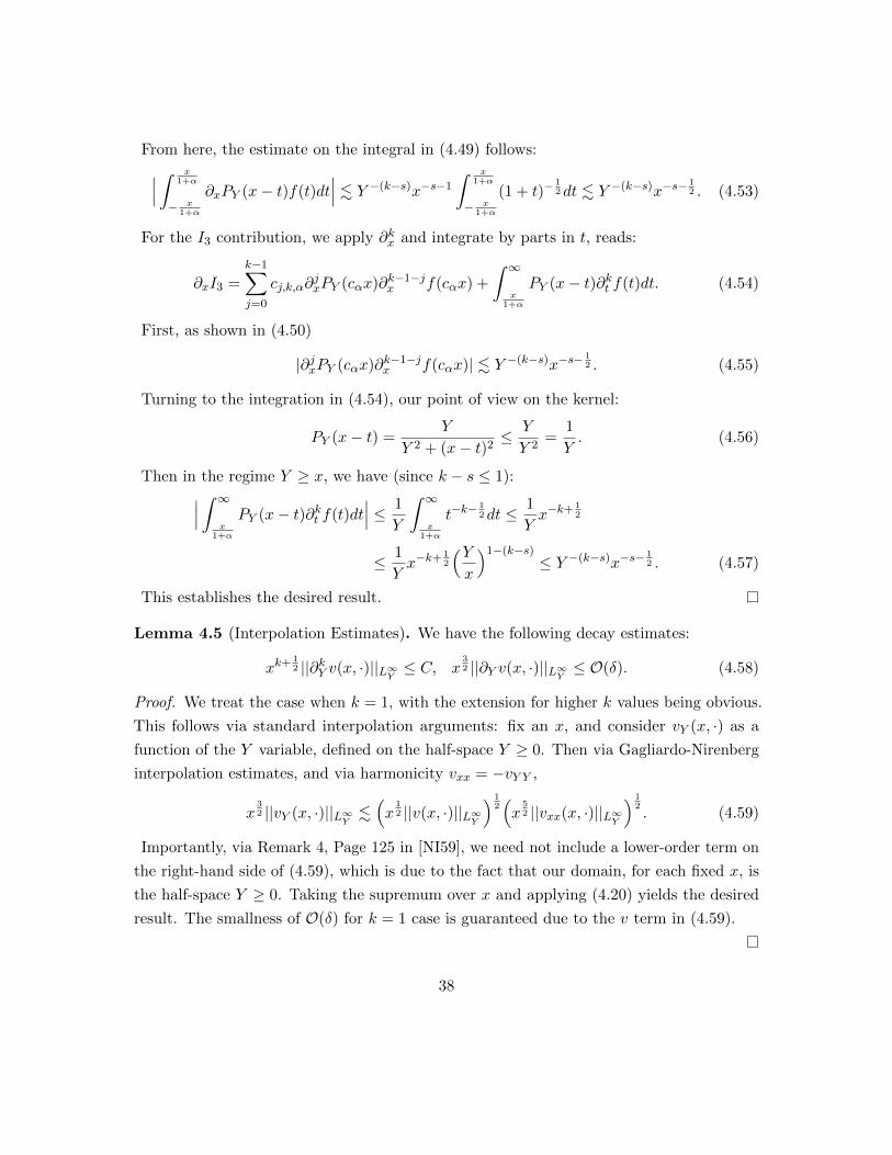
Lemma 4.5 (Interpolation Estimates). We have the following decay estimates:

xk+ 12 ||∂kY v(x, ·)||L∞Y ≤ C, x

32 ||∂Y v(x, ·)||L∞Y ≤ O(δ). (4.58)

Proof. We treat the case when k = 1, with the extension for higher k values being obvious.

This follows via standard interpolation arguments: fix an x, and consider vY (x, ·) as a

function of the Y variable, defined on the half-space Y ≥ 0. Then via Gagliardo-Nirenberg

interpolation estimates, and via harmonicity vxx = −vY Y ,

x32 ||vY (x, ·)||L∞Y .

(x

12 ||v(x, ·)||L∞Y

) 12(x

52 ||vxx(x, ·)||L∞Y

) 12. (4.59)

Importantly, via Remark 4, Page 125 in [NI59], we need not include a lower-order term on

the right-hand side of (4.59), which is due to the fact that our domain, for each fixed x, is

the half-space Y ≥ 0. Taking the supremum over x and applying (4.20) yields the desired

result. The smallness of O(δ) for k = 1 case is guaranteed due to the v term in (4.59).

38

Proposition 4.6 (Euler Correctors). Suppose [u1e, v

1e ] solves the boundary value problem:

∆v1e = 0, v1

e(x, 0) = −v0p(x, 0), u1

e =

∫ ∞x

v1eY (x′, Y )dx′, for x ≥ 1. (4.60)

Then the following bounds holds for any k, j ≥ 0:

supY≥0

∣∣∣∂kx∂jY v1e

∣∣∣xk+j+ 12 ≤ C, sup

Y≥0

[∣∣∣u1e, v

1e

∣∣∣x 12 +

∣∣∣u1ex, v

1eY

∣∣∣x 32

]≤ O(δ). (4.61)

Proof. We shall take v1e = v from the above lemmas. For the u1

e profile, we define for x ≥ 1:

u1e(x, Y ) :=

∫ ∞x

v1eY (x′, Y )dx′. (4.62)

From here it is clear that the Cauchy-Riemann equations hold:

u1ex = −v1

eY , u1eY =

∫ ∞x

v1eY Y = −

∫ ∞x

v1exx = v1

ex. (4.63)

We have used that v1ex(x, Y )→ 0 as x→∞. From Lemma 4.5, it is then clear that:∣∣∣u1

e

∣∣∣ =∣∣∣ ∫ ∞

xu1exdx

′∣∣∣ =

∣∣∣ ∫ ∞x

v1eY dx

′∣∣∣ ≤ O(δ)

∫ ∞x|x′|−

32dx′ ≤ O(δ)x−

12 . (4.64)

Remark 4.7 (In-flow Conditions). Note that we do not solve for the Euler correctors

given an arbitrary in-flow condition at x = 1. Rather, we take [u1e, v

1e , P

1e ] to be the explicit

profiles obtained by applying the Poisson extension to f . In this sense, the set-up we

consider here is distinct from the construction of Euler profiles in [GN14].

5 Prandtl Layer 1

5.1 Derivation of Linearized Prandtl Equations:

In this section, we will construct the Prandtl correctors, [u1p, v

1p, P

1p ]. Let us now obtain the

equations that they will satisfy. We do this in a manner which can be easily generalized in

the next section. We expand the nonlinear terms:

u(1)s u(1)

sx =(u(0)s +

√εu1e +√εu1p

)(u(0)sx +

√εu1ex +

√εu1px

)= u(0)

s u(0)sx +

√εu(1)sx u

1p +√εu(1)s u1

px + εu1pu

1px +

√εu1exu

0p +√εu1eu

0px

39

+√εu1ex + εu1

eu1ex, (5.1)

v(1)s u(1)

sy =(v0p + v1

e +√εv1p

)(u0py + εu1

eY +√εu1py

)= v(1)

s u0py +

√εu(1)sy v

1p +√εv(1)s u1

py + εv1pu

1py + εv0

pu1eY + εv1

eu1eY , (5.2)

u(1)s v(1)

sx =(

1 + u0p +√εu1e +√εu1p

)(v0px + v1

ex +√εv1px

)= u(0)

s v0px +

√εv1pxu

(1)s +

√εv(1)sx u

1p + εu1

pv1px + u0

pv1ex +

√εu1ev

0px

+ v1ex +

√εu1ev

1ex, (5.3)

v(1)s v(1)

sy =(v0p + v1

e +√εv1p

)(v0py +

√εv1eY +

√εv1py

)= v0

pv0py +

√εv1pyv

(1)s +

√εv(1)sy v

1p + εv1

pv1py +

√εv0pv

1eY + v1

ev0py +

√εv1ev

1eY . (5.4)

Let us now denote:

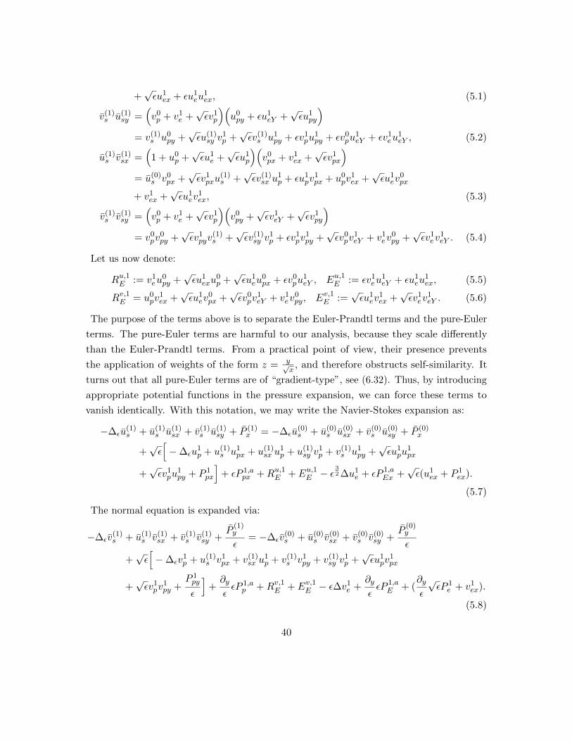
Ru,1E := v1eu

0py +

√εu1exu

0p +√εu1eu

0px + εv0

pu1eY , Eu,1E := εv1

eu1eY + εu1

eu1ex, (5.5)

Rv,1E = u0pv

1ex +

√εu1ev

0px +

√εv0pv

1eY + v1

ev0py, Ev,1E :=

√εu1ev

1ex +

√εv1ev

1eY . (5.6)

The purpose of the terms above is to separate the Euler-Prandtl terms and the pure-Euler

terms. The pure-Euler terms are harmful to our analysis, because they scale differently

than the Euler-Prandtl terms. From a practical point of view, their presence prevents

the application of weights of the form z = y√x, and therefore obstructs self-similarity. It

turns out that all pure-Euler terms are of “gradient-type”, see (6.32). Thus, by introducing

appropriate potential functions in the pressure expansion, we can force these terms to

vanish identically. With this notation, we may write the Navier-Stokes expansion as:

−∆εu(1)s + u(1)

s u(1)sx + v(1)

s u(1)sy + P (1)

x = −∆εu(0)s + u(0)

s u(0)sx + v(0)

s u(0)sy + P (0)

x

+√ε[−∆εu

1p + u(1)

s u1px + u(1)

sx u1p + u(1)

sy v1p + v(1)

s u1py +

√εu1pu

1px

+√εv1pu

1py + P 1

px

]+ εP 1,a

px +Ru,1E + Eu,1E − ε32 ∆u1

e + εP 1,aEx +

√ε(u1

ex + P 1ex).

(5.7)

The normal equation is expanded via:

−∆εv(1)s + u(1)

s v(1)sx + v(1)

s v(1)sy +

P(1)y

ε= −∆εv

(0)s + u(0)

s v(0)sx + v(0)

s v(0)sy +

P(0)y

ε

+√ε[−∆εv

1p + u(1)

s v1px + v(1)

sx u1p + v(1)

s v1py + v(1)

sy v1p +√εu1pv

1px

+√εv1pv

1py +

P 1py

ε

]+∂yεεP 1,a

p +Rv,1E + Ev,1E − ε∆v1e +

∂yεεP 1,a

E + (∂yε

√εP 1

e + v1ex).

(5.8)

40

In the above expressions, the [u(0)s , v

(0)s ], [u

(1)s , v

(1)s ] are known at this stage, and the u1

p, v1p

are unknowns, to be constructed in this step. Similarly for the pressures, the the P 1e is

known, but the auxiliary pressures P 1,aE , P 1,a

p are to be defined in this section. Finally, as

can be seen from the definitions in (5.5), (5.6), the Ru,1E , Rv,1E , Eu,1E , Ev,1E are all knowns. Let

us now simplify the above expressions. First, via the construction of [u0p, v

0p] we may write:

Ru,0 := −∆εu(0)s + u(0)

s u(0)sx + v(0)

s u(0)sy + P (0)

x + v1eu

0py

= −εu0pxx +

√εyv1

eY u0py + εu0

py

∫ y

0

∫ y′

yv1eY Y dy

′′dy′. (5.9)

This then accounts for the lowest order term from Ru,1E in (5.5), allowing us to redefine:

Ru,1E =√εu1exu

0p +√εu1eu

0px + εv0

pu1eY . (5.10)

Let us now define the auxiliary Euler pressure:

P 1,aE := −1

2

(∣∣∣u1e

∣∣∣2 +∣∣∣v1e

∣∣∣2), (5.11)

so that, combined with the equations we have taken for [u1e, v

1e ], we have:

Lemma 5.1. With P 1,aE as in (5.11), and Eu,1E , Ev,1E as in (5.5) - (5.6),

∂xεP1,aE + Eu,1E =

∂yεεP 1,a

E + Ev,1E = 0. (5.12)

Remark 5.2. Denoting by ∇ε := (∂x,∂Y√ε), the above lemma reads:

∇εεP 1,aE + (Eu,1E , Ev,1E ) = 0. (5.13)

Thus, the purely Eulerian terms are of gradient structure, which is then exploited with

the introduction of our auxiliary pressure.

Proof. The proof follows by direct calculation and an appeal to (4.5):

ε∂xP1,aE = −εu1

eu1ex − εv1

ev1ex = −εu1

eu1ex − εv1

eu1eY = −Eu,1E . (5.14)

Similarly,

∂Y√εεP 1,a

E = −√εu1eu

1eY − εv1

ev1eY = −

√εu1ev

1ex − εv1

ev1eY = −Ev,1E . (5.15)

The claim has been proven.

41

Corollary 5.3. All “purely Eulerian” terms from the expansions (5.7), (5.8) vanish identi-

cally. That is:

Eu,1E − ε32 ∆u1

e + εP 1,aEx +

√ε(u1

ex + P 1ex) = 0, (5.16)

Ev,1E − ε∆v1e +

∂yεεP 1,a

E + (∂yε

√εP 1

e + v1ex) = 0. (5.17)

Proof. First, by harmonicity of [u1e, v

1e ], we have:

ε32 ∆u1

e = ε∆v1e = 0. (5.18)

Next, regarding the final terms in both (5.7) and (5.8), by the equations (4.2) and (4.4),

we see that these terms drop out:

u1ex + P 1

ex = 0, v1ex + P 1

eY = 0. (5.19)

Coupled with (5.12), this establishes the desired claim.

In the above calculation, we are using crucially the Cauchy-Riemann structure of [u1e, v

1e ]

in 4.7; harmonicity alone does not suffice here. Next, define the auxiliary Prandtl pressure:

P 1,ap :=

∫ ∞y

[−∆εv

(0)s + u(0)

s v(0)sx + v(0)

s v(0)sy

]+

∫ ∞y

Rv,1E . (5.20)

Combining all this, we take our Prandtl-1 equation to be:

−u1pyy + (1 + u0

p)u1px + u(1)

sx u1p + u0

py

(v1p − v1

p(x, 0))

+ v(1)s u1

py + P 1px = f (1), (5.21)

together with the divergence free condition u1px + v1

py = 0, and the boundary conditions:

u1p(x, 0) = 0, lim

y→∞[u1p(x, y), v1

p(x, y)] = 0, v1p(x, 0) = −v2

e(x, 0), u1p(1, y) = U1(y). (5.22)

Here, the forcing term is defined as:

f (1) := ε−12

[Ru,0 +Ru,1E + εP 1,a

px

]. (5.23)

The boundary contribution of v1p(x, 0) in (5.21) again arises from the calculation:

v2e(x, Y )u0

py = v2e(x, 0)u0

py +√εyu0

pyv2eY + εu0

py

∫ y

0

∫ y′

yv2eY Y

42

= −v1p(x, 0)u0

py +√εyu0

pyv2eY + εu0

py

∫ y

0

∫ y′

yv2eY Y . (5.24)

Consolidating (5.18), (5.19), (5.12), (5.20), (5.21), (5.24) with the expressions (5.7) and

(5.8) then shows that the following remainder is contributed:

Ru,1 =√ε[− εu1

pxx +√εyv2

eY u0py + εu0

py

∫ y

0

∫ y′

yv2eY Y + (εu1

eY +√εu1py)v

1p (5.25)

+√ε(u1

e + u1p)u

1px

],

Rv,1 =√ε[−∆εv

1p + u(1)

s v1px + v(1)

sx u1p + v(1)

s v1py + v(1)

sy v1p +√εu1pv

1px +

√εv1pv

1py

]. (5.26)

Let us emphasize the boundary condition at y →∞ for v1p means that we will define:

v1p(x, y) =

∫ ∞y

u1px(x, y′)dy′. (5.27)

We may evaluate the equation (5.21) at y =∞ to see that the pressure term drops out.

That is the pressure in the Prandtl layer is constant, so we may WLOG take P 1p = 0.

5.2 Global in x Existence and Decay:

The first step is to homogenize the boundary conditions by introducing the new unknowns:

u = u1p + χ(y)u1

e(x, 0), v = v1p − v1

p(x, 0) + u1ex(x, 0)Iχ(y), Iχ(y) =

∫ ∞y

χ(θ)dθ, (5.28)

where χ(y) is a cutoff function satisfying:

χ(0) = 1, ∂kyχ(0) = 0,

∫ ∞0

χ(y)dy = 0. (5.29)

The mean-zero condition is meant to ensure that v(0) = 0. The homogenized profiles now

satisfy the following system:

(1 + u0p)ux − uyy + P(u, v) = f (1) + J ; u(x, 0) = v(x, 0) = 0, lim

y→∞u(x, y) = 0. (5.30)

along with the divergence free condition ux + vy = 0. Here:

P := u(1)sx u+ u0

pyv + v(1)s uy, (5.31)

J := u(1)s χ(y)u1

ex(x, 0)− χ′′u1e(x, 0)− χ(y)u(1)

sx u1e(x, 0)− u0

pyIχ(y)u1ex(x, 0)

43

+ v(1)s χ′(y)u1

e(x, 0). (5.32)

We note that v(x, y) does not vanish as y → ∞ due to the definition in (5.28). The

essential feature of v(x, y) that will be in use is that v(x, 0) = 0. Examining (5.31), one

observes that v is always accompanied by u0p, which decays rapidly in y for each fixed x.

Let us now define the norm in which we shall control the Prandtl solutions:

||u||2P (X1,σ) := sup1≤x≤X1

∫u2x−2σ + u2

yx1−2σ+

∫ X1

1

∫u2x−1−2σ + u2

yx−2σ + u2

xx1−2σ.

(5.33)

We shall also need the following, differentiated version, of the above Prandtl-layer norm:

||u||2Pk(X1,σ) := sup1≤x≤X1

∫|∂kxu|2x2k−2σ + |∂kxuy|2x2k+1−2σ (5.34)

+

∫ X1

1

∫|∂kxu|2x2k−1−2σ + |∂kxuy|2x2k−2σ + |∂k+1

x u|2x2k+1−2σ.

Through the H1y → L∞y embedding, it is clear that:

sup1≤x≤X1

xk+ 14−σ||∂kxu||L∞ ≤ ||u||Pk(X1,σ). (5.35)

Finally, we shall write the global norms as:

||u||P (σ) := ||u||P (∞,σ), ||u||Pk(σ) := ||u||Pk(∞,σ). (5.36)

Remark 5.4. A comparison of the norms Pk with the estimates valid for [u0p, v

0p] in (3.86),

(3.91) show that u1p is roughly “x−

14 -better” than u0

p. There is no front-profile as in the case

of [u0p, v

0p], which is because the present boundary condition, u1

p(x, 0) = −u1e(x, 0) decays

as x→∞, due to (4.64), in contrast with the boundary condition for u0p(x, 0) = −δ. The

secondary reason is because f (1) in (5.23) contains derivative and nonlinear terms from the

previous layers, which enhances the decay in x.

The first step is to give the following estimates on the forcing terms, which capitalize on

the structure of these terms either having many derivatives (thereby enhancing decay in x)

or are of product form (also enhancing decay in x):

Lemma 5.5 (Forcing Estimates). For any k,m ≥ 0, and arbitrary N > 0∣∣∣zm∂kxJ ∣∣∣ ≤ C(k,m)〈y〉−Nx−k−12 , (5.37)

||zm∂kxf (1)||L2y≤ C(k,m)〈x〉−k−

54 . (5.38)

44

Proof. The estimate for the J terms is direct, thanks to Proposition 4.6, estimate (4.61).

For f (1), in consultation with the definition (5.23), we start with the Ru,0, defined in (5.9):

√ε||u0

pxx||L2y.√εx−

74 , (5.39)

||yu0pyv

1eY ||L2

y≤ ||x−

14 yu0

py||L2y

supy

∣∣∣v1eY

∣∣∣x 14 . x−

54 , (5.40)

√ε||u0

py

∫ y

0

∫ y′

yv1exxdy

′′dy′||L2y≤√ε||y2u0

py||L2y||v1

exx||L∞y .√εx−

74 . (5.41)

Second, we control Ru,1E via:

ε−12 ||Ru,1E ||L2

y≤ ||u1

ex||L∞y ||u0p||L2

y+ ||u1

e||L∞y ||u0px||L2

y+√ε||v0

p||L2y||u1

eY ||L∞y. x−

54 . (5.42)

Next, according to (5.20), we have:

||P 1,apx ||L2

y≤ ||〈y〉

32

+κ∂x

(−∆εv

(0)s + u(0)

s v(0)sx + v(0)

s v(0)sy

)||L∞y + ||〈y〉

32

+κRv,1Ex||L∞y . (5.43)

For each of these terms, the ability to trade x34

+κ2 for y

32

+κ is in constant use:

||〈y〉32

+κ∆εv0px||L∞y + ||〈y〉

32

+κ∂xu(0)s v(0)

sx ||L∞y + ||〈y〉32

+κ∂xv(0)s v(0)

sy ||L∞y+ ||〈y〉

32

+κ∂xu0pv

1ex||L∞y + ||〈y〉

32

+κ∂x√εu1ev

0px||L∞y + ||〈y〉

32

+κ∂x√εv0pv

1eY ||L∞y

+ ||〈y〉32

+κ∂xv1ev

0py||L∞y . x−

32 . (5.44)

Above, we are using the established estimates in (3.86), (3.91) for the Prandtl-0 profiles,

and (4.61) for the Euler-1 profiles. The desired estimates are proven for m = 0. For general

m the estimates work in an identical manner, after noticing that powers of z play no role

when accompanied by [u0p, v

0p], which appear in every term above.

The above lemma relies crucially on Corollary 5.3 in order to apply the weight zm. We

now give the following energy estimate:

Lemma 5.6. Let σ > 0 and fix any X1 > 1. Then:

supx∈[1,X1]

∫x−2σu2 +

∫ X1

1

∫x−1−2σu2 +

∫ X1

1

∫x−2σu2

y

. O(δ;σ)

∫ X1

1

∫v2yx

1−2σ + C(σ). (5.45)

The constant above depends poorly on small σ.

45

Remark 5.7. The need for this σ > 0 is to avoid certain x-integrations being critical. We

make the notational convention that we will not rename different values for σ (for instance

2σ), as we can always redefine σ to be smaller. However, within a single calculation (for

instance the upcoming proof) we fix a σ > 0.

Proof. Applying the multiplier M = ux−2σ to the system (5.30) gives the following terms:∫ ((1+u0

p)∂x−∂yy)u·ux−2σ & ∂x

∫(1+u0

p)x−2σu2+

∫x−1−2σu2+

∫x−2σu2

y−∫u0pxu

2x−2σ.

(5.46)

The constant in the above estimate depends poorly on σ, as there is a factor of σ

accompanying the∫x−1−2σu2 term. The final term above then gets placed into the

contributions from P, to which we now turn (see the definition in (5.31)):∣∣∣ ∫ P · ux−2σ∣∣∣ ≤ ||xu(1)

sx , yu0py, v

(1)sy x||∞

(∫u2x−1−2σ +

∫v2yx

1−2σ)

≤ O(δ)(∫

u2x−1−2σ +

∫v2yx

1−2σ). (5.47)

Above, we have used the Prandtl-0 bounds in (3.86), which crucially provides the smallness

of u0px, u

0py in terms of O(δ). No smallness of Eulerian profiles is required due to the extra

factor of√ε. The key estimate which forces a loss of ∂x derivative is the following:∣∣∣ ∫ u0

pyv · ux−2σ∣∣∣ ≤ ||u0

pyy||L∞∫ ∣∣∣v

yux−2σ

∣∣∣ ≤ O(δ)||vyx12−σ||L2

y||ux−

12−σ||L2

y. (5.48)

The structure of the key estimate above, (5.48), is omnipresent in our analysis: we use

the y-absorption of u0py to produce a vy term via Hardy’s inequality (which is valid as

v(x, 0) = 0). This then forces a loss of x12−σ in the decay, which must then be regained in

the next lemma. Again, the estimate ||yu0py||L∞ ≤ O(δ) arises from (3.86). Next, we arrive

at the forcing terms. First, via (5.37):∣∣∣ ∫ J · ux−2σ∣∣∣ . ∫ 〈y〉−Nx− 1

2 |u|x−2σ . ||x−12−σ〈y〉−

N2 ||L2

y||x−σ u

〈y〉N2

||L2y

≤ 1

100, 000||uyx−σ||2L2

y+ Cx−1−2σ. (5.49)

Upon taking an integration in dx, the majorizing terms above are finite. Next, according

to (5.38), via Young’s inequality:∣∣∣ ∫ f (1) · ux−2σ∣∣∣ ≤ ||f (1)x

12−σ||L2

y||ux−

12−σ||L2

y≤ Cx−

32 +

1

100, 000

∫u2x−1−2σdy.

46

Placing these estimates together:

∂x

∫x−2σu2 +

∫x−1−2σu2 +

∫x−2σu2

y . O(δ)

∫u2xx

1−2σ + x−1−2σ.

Integrating above from x = 1 to x = X1 yields:∫X−2σ

1 u2(X1)dy +

∫ X1

1

∫x−1−2σu2 +

∫ X1

1

∫x−2σu2

y

. O(δ)

∫ X1

1

∫v2yx

1−2σ + C. (5.50)

Finally, we reason as follows: the second and third terms on the left-hand side above are

positive, which then gives for this X1:∫X−2σ

1 u2(X1)dy . O(δ)

∫ X1

1

∫v2yx

1−2σ + C. (5.51)

For any X2 ∈ [1, X1], the same estimate holds, namely:∫X−2σ

2 u2(X2)dy . O(δ)

∫ X2

1

∫v2yx

1−2σ + C . O(δ)

∫ X1

1

∫v2yx

1−2σ + C. (5.52)

Above, we have used the monotonicity of the right-hand side as X2 < X1. This allows us

to replace in (5.50) the first term on the left-hand side with sup1≤x≤X1

∫x−2σu2dy. This

then gives the desired estimate in (5.45).

We now recover the vy term on the right-hand side of (5.45) via:

Lemma 5.8. Let σ > 0, and fix any X1 > 1. Then:

sup1≤x≤X1

∫u2yx

1−2σ +

∫ X1

1

∫u2xx

1−2σ . C +O(δ)

∫ X1

1

∫u2x−1−2σ

+

∫ X1

1

∫u2yx−2σ. (5.53)

Proof. We now apply the multiplier M = uxx1−2σ to the system in (5.30). Doing so yields

the following positive terms:∫ ((1 + u0

p)∂x − ∂yy)u · uxx1−2σ & ∂x

∫u2yx

1−2σ −∫u2yx−2σ +

∫u2xx

1−2σ. (5.54)

47

Note crucially that the middle term in the above estimate, ||uyx−σ||2L2y, has been estimated

in (5.45) upon taking an x-integration. To close this sequence of estimates, therefore, it is

crucial that this small parameter O(δ) is attached to the ||vyx12−σ||2L2 term in (5.45). Next,

we come to the profile terms, P (see (5.31) for the definition):∣∣∣ ∫ P · uxx1−2σ∣∣∣ ≤ ||xu(1)

sx , yu0py, v

(1)s x

12 ||L∞

(||ux−

12−σ||2L2

y+ ||uxx

12−σ||2L2

y

)≤ O(δ)

(||ux−

12−σ||2L2

y+ ||uxx

12−σ||2L2

y

). (5.55)

We have used estimates (3.86), (3.91), and (4.61), which provide the smallness of O(δ).

Next, we come to f (1), for which we use the estimate in (5.38) (with k = 0):∣∣∣ ∫ f (1)uxx1−2σ

∣∣∣ ≤ ||x 12−σf (1)||L2

y||uxx

12−σ||L2

y≤ Cx−

32 +

1

100, 000||uxx

12−σ||2L2

y. (5.56)

Piecing the above estimates together gives:

∂x

∫u2yx

1−2σ +

∫u2xx

1−2σ

≤∫u2yx−2σ +O(δ)

∫u2x−1−2σ + Cx−1−σ +

∫J · uxx1−2σ. (5.57)

Now, we take an integration from x = 1 to x = X1:∫u2y(X1)X1−2σ

1 +

∫ X1

1

∫u2xx

1−2σ .∫ X1

1

∫u2yx−2σ

+O(δ)

∫ X1

1

∫u2x−1−2σ + C +

∫ X1

1

∫J · uxx1−2σ. (5.58)

The last step is to come to the terms in J , from (5.32). The most delicate term here

requires successive integration by parts:∫ X1

1

∫χ′′(y)x1−2σu1

e(x, 0)ux (5.59)

= −∫ X1

1

∫χ′′(y)u∂xu1

e(x, 0)x1−2σ −∫x=1

u1e(1, 0)uχ′′(y)dy

+

∫x=X1

X1−2σ1 u1

e(X1, 0)χ′′(y)u(X1, y)dy (5.60)

= −∫ X1

1

∫χ′′(y)u∂xu1

e(x, 0)x1−2σ+ C

−∫x=X1

X1−2σ1 u1

e(X1, 0)χ′(y)uy(X1, y)dy (5.61)

48

≤∫ X1

1

∫χ′(y)uy∂xu1

e(x, 0)x1−2σ+ C +1

100, 000

∫x=X1

X1−2σ1 u2

y(X1) (5.62)

. ||uyx−σ||L2 ||χ′(y)x−12−σ||L2 + C ≤ C +

1

100, 000||uyx−σ||2L2 . (5.63)

Going from (5.61) to (5.62), we have used |u1e(X1, 0)| . X

− 12

1 , according to (4.61). Going

from (5.62) to (5.63), we have used |u1ex(x, 0)| . x

32 , also according to (4.61). Finally, we

have absorbed the boundary contribution at x = X1,∫u2yX

1−2σ1 into the left-hand side of

(5.58). A consultation with (5.32) shows that we can perform a similar calculation with

the remaining terms in J because these terms either have one extra x-derivative, or are

accompanied by v(1)s , which contributes additional decay of x−

12 . This then gives:∫

u2y(X1)X1−2σ

1 +

∫ X1

1

∫u2xx

1−2σ .∫ X1

1

∫u2yx−2σ +O(δ)

∫ X1

1

∫u2x−1−2σ + C.

Using a similar line of reasoning as in the Lemma 5.6, we can replace the∫u2y(X1)X1−2σ

1

with the supremum over all x ∈ [1, X1], thereby yielding the desired result.

Consolidating the results of the previous two lemmas and applying contraction mapping:

Corollary 5.9. For δ, ε sufficiently small relative to σ, a solution to the Prandtl system in

(5.30) satisfies the following a-priori estimate in the space P :

||u||2P (X1,σ) . C(σ). (5.64)

For δ, ε sufficiently small, there exists a unique solution to (5.30), satisfying ||u||P (X1) ≤ C(σ).

The constant above in (5.64) is independent of X1, and so we can immediately send X1 →∞,

thereby yielding a global solution on x ∈ [1,∞) satisfying: ||u||P ≤ C(σ).

It is possible to successively differentiate the system in ∂x, and re-apply the previous

estimates, noting that the added x−derivative adds a factor of x−1 to each term above,

enabling us to enhance the multiplier to [xk−2σ∂kxu, x1+k−2σ∂k+1

x u]. This is the reason for

the differentiated version of the Prandtl-norm in (5.34). To do so, we simply need:

Lemma 5.10 (Initial Conditions). For each k ≥ 0, the initial data ∂kxu(1, y) is of order δ

and decays rapidly in y.

49

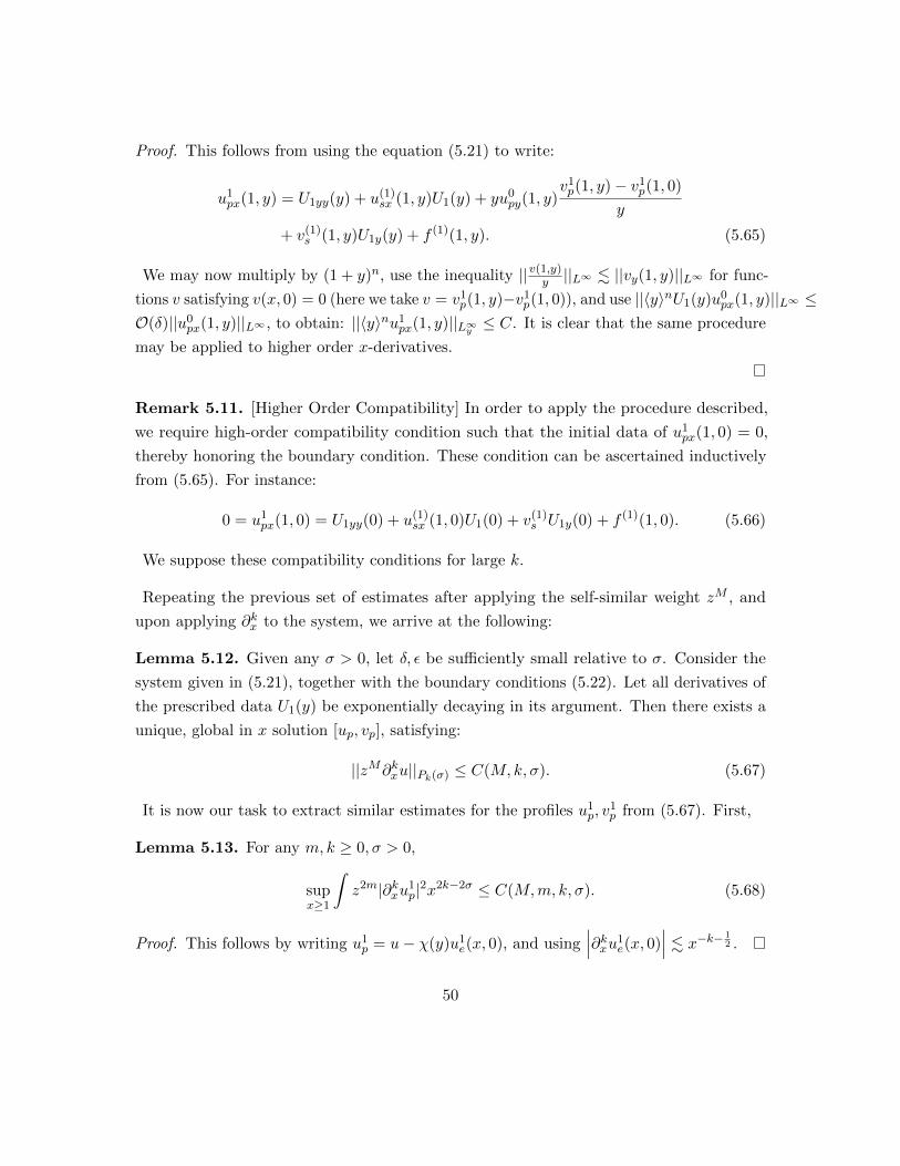
Proof. This follows from using the equation (5.21) to write:

u1px(1, y) = U1yy(y) + u(1)

sx (1, y)U1(y) + yu0py(1, y)

v1p(1, y)− v1

p(1, 0)

y

+ v(1)s (1, y)U1y(y) + f (1)(1, y). (5.65)

We may now multiply by (1 + y)n, use the inequality ||v(1,y)y ||L∞ . ||vy(1, y)||L∞ for func-

tions v satisfying v(x, 0) = 0 (here we take v = v1p(1, y)−v1

p(1, 0)), and use ||〈y〉nU1(y)u0px(1, y)||L∞ ≤

O(δ)||u0px(1, y)||L∞ , to obtain: ||〈y〉nu1

px(1, y)||L∞y ≤ C. It is clear that the same procedure

may be applied to higher order x-derivatives.

Remark 5.11. [Higher Order Compatibility] In order to apply the procedure described,

we require high-order compatibility condition such that the initial data of u1px(1, 0) = 0,

thereby honoring the boundary condition. These condition can be ascertained inductively

from (5.65). For instance:

0 = u1px(1, 0) = U1yy(0) + u(1)

sx (1, 0)U1(0) + v(1)s U1y(0) + f (1)(1, 0). (5.66)

We suppose these compatibility conditions for large k.

Repeating the previous set of estimates after applying the self-similar weight zM , and

upon applying ∂kx to the system, we arrive at the following:

Lemma 5.12. Given any σ > 0, let δ, ε be sufficiently small relative to σ. Consider the

system given in (5.21), together with the boundary conditions (5.22). Let all derivatives of

the prescribed data U1(y) be exponentially decaying in its argument. Then there exists a

unique, global in x solution [up, vp], satisfying:

||zM∂kxu||Pk(σ) ≤ C(M,k, σ). (5.67)

It is now our task to extract similar estimates for the profiles u1p, v

1p from (5.67). First,

Lemma 5.13. For any m, k ≥ 0, σ > 0,

supx≥1

∫z2m|∂kxu1

p|2x2k−2σ ≤ C(M,m, k, σ). (5.68)

Proof. This follows by writing u1p = u− χ(y)u1

e(x, 0), and using∣∣∣∂kxu1

e(x, 0)∣∣∣ . x−k−

12 .

50

Next, we may give the following uniform decay estimate for v1p:

Corollary 5.14 (Uniform Estimates for v1p). For any m ≥ 0,

||zm∂kxv1p||L∞y . x−k−

34

+σC(σ,m, k). (5.69)

Proof. First, according to (5.27), we have the rapid decay v1p → 0 as y → ∞. By the

divergence-free condition, and the trace inequality, and for any small κ > 0,∣∣∣v1p

∣∣∣2 .∣∣∣ ∫ ∞

yv1pvpy

∣∣∣ ≤ ∫ ∞0

∣∣∣ v1p

y12−κy

12−κv1

py

∣∣∣ ≤ || v1p

y12−κ||L2

y||y

12−κv1

py||L2y

(5.70)

≤ ||y12

+κv1py||L2

y||y

12−κv1

py||L2y

= ||x14

+κz12

+κv1py||L2

y||x

14−κz

12−κv1

py||L2y

(5.71)

≤ x12x−1+σx−1+σ = x−

32

+2σ. (5.72)

We have used the κ > 0 to avoid the critical Hardy inequality. The Hardy inequality we

have used (with power y−12

+κv1p) relies on the vanishing of v1

p at y = ∞. From here the

desired bound follows for m = 0, k = 0, and k,m ≥ 1 works analogously.

The final ingredient we will need is to understand the connection between the norms we

have controlled, Pk, and the quantities u1py, u

1pyy. This is the content of the following:

Lemma 5.15.

x34−σ||zmu1

py||L∞y + x12−σ||zmu1

py||L2y

+ x1−σ||zmu1pyy||L2

y≤ C <∞. (5.73)

Proof. First, let us record:

x1−2σ

∫z2m

∣∣∣u1py

∣∣∣2 ≤ x1−2σ

∫z2mu2

y + x1−2σ

∫z2mχ2|u1

e|2(x, 0)

≤ ||zmu||P (σ) + C. (5.74)

Via the equation (5.21), we have:

x1−σ||u1pyy||L2

y≤ x1−σ||u1

px||L2y

+ x1−σ||P||L2y

+ x1−σ||f (1)||L2y

. ||u||P1(σ) + ||u||P (σ) + C. (5.75)

We are using the decay rates established for u0p in (3.86), and the pointwise decay of the

Euler profiles established in (4.48) and the relations in (5.68). Let us give P in detail,

x1−σ||u(1)sx u

1p||L2

y≤ ||xu(1)

sx ||L∞x−σ||u1p||L2

y≤ O(δ)||u||P +O(δ), (5.76)

51

x1−σ||u0py

(v1p(x, y)− v1

p(x, 0))||L2

y≤ x1−σ||yu0

py||L∞ ||v1p(x, y)− v1

p(x, 0)

y||L2

y

≤ O(δ)x1−σ||u1px||L2

y≤ O(δ)||u||P1 , (5.77)

x1−σ||v(1)s u1

py||L2y≤ ||x

12 v(1)s ||L∞x

12−σ||u1

py||L2y≤ O(δ)||u||P +O(δ). (5.78)

For the final line we have used (5.74). Next, via Sobolev interpolation in the y direction,

x34−σ||u1

py||L∞y ≤(x1−σ||u1

pyy||L2y

) 12(x

12−σ||u1

py||L2y

) 12 ≤ C||u||P +

1

100x1−σ||u1

pyy||L2y.

(5.79)

Coupled with the u1pyy estimate in (5.75), this then establishes the desired bounds. The

weighted estimate in z follows analogously.

We will select now,

σ = σ1 =3

3n × 10, 000. (5.80)

Summarizing the results of this section:

Proposition 5.16 (Prandtl-1 Layer Bounds). Given any n ∈ N, let σ1 be as in (5.80),

and let δ, ε be sufficiently small relative to n and σ1. Consider the system given in (5.21),

together with the boundary conditions (5.22). Let all derivatives of the prescribed data

U0(y) be exponentially decaying in its argument. Then there exists a unique, global in x

solution [u1p, v

1p], satisfying:

||zM∂kxu1p||Pk(σ1) + xk+ 3

4−σ1 ||zm∂kxv1

p||L∞y ≤ C(M,k, n), for any k,m ≥ 0. (5.81)

6 Intermediate Layers

We now construct intermediate layers i = 2 through i = n− 1. This is achieved inductively,

starting with the construction of the Euler Layer, uie, vie. Let us fix the parameters:

σi =3i

3n × 10, 000for i = 2, ..., n. (6.1)

The reason for this selection will be seen in (10.55).

52

6.1 Construction of Euler Layer, [uie, vie]

For this step in the construction, we suppose that [u(i−1)s , v

(i−1)s ] have already been con-

structed. The inductive hypothesis on the 1, ..., i− 1 Prandtl profiles are as follows:

||zm∂kxujp||Pk(σj) ≤ C(k,m, n), for j = 1, ..., i− 1, (6.2)

where [ujp, vjp] satisfy the system given in (6.48) for 2 ≤ j ≤ i − 1, and for i = 2, that

[u1p, v

1p] satisfy (5.21). In order to obtain the equations for [uie, v

ie], we expand the nonlinear

terms including the new Euler terms:

u(i)s u

(i)sx =

(u(i−1)s + ε

i2uie

)(u(i−1)sx + ε

i2uiex

)= u(i−1)

s u(i−1)sx + ε

i2 u(i−1)

sx uie + εi2 u(i−1)

s uiex + εiuieuiex, (6.3)

v(i)s u(i)

sy =(v(i−1)s + ε

i−12 vie

)(u(i−1)sy +

√εε

i2uieY

)= v(i−1)

s u(i−1)sy + ε

i−12 u(i−1)

sy vie +√εε

i2 v(i−1)s uieY + εivieu

ieY . (6.4)

u(i)s v

(i)sx =

(u(i−1)s + ε

i2uie

)(v(i)sx + ε

i−12 viex

)= u(i−1)

s v(i−1)sx + ε

i2 v(i−1)sx uie + ε

i−12 u(i−1)

s viex + εi−12uiev

iex, (6.5)

v(i)s v(i)

sy =(v(i−1)s + ε

i−12 vie

)(v(i−1)sy + ε

i2 vieY

)= v(i−1)

s v(i−1)sy + ε

i−12 v(i−1)

sy vie + εi2 v(i−1)s vieY + εi−

12 viev

ieY . (6.6)

We will now define several terms:

Definition 6.1. The i− 1’th remainder is denoted by:

Ru,i−1 := −∆εu(i−1)s + u(i−1)

s u(i−1)sx + v(i−1)

s u(i−1)sy + P (i−1)

sx + εi−12 vieu

0py, (6.7)

Rv,i−1 := −∆εv(i−1)s + u(i−1)

s v(i−1)sx + v(i−1)

s v(i−1)sy +

∂yεP (i−1)s . (6.8)

We will also split the Euler-Euler interaction terms and the Euler-Prandtl terms via:

Definition 6.2.

Ru,iE := εi2uiex

[ i−1∑j=0

εj2ujp

]+ ε

i2uie

[ i−1∑j=0

εj2ujpx

]

+ εi2√εuieY

[ i−1∑j=0

εj2 vjp

]+ ε

i−12 vie

[ i−1∑j=1

εj2ujpy

], (6.9)

53

Rv,iE := εi−12 viex

i−1∑j=0

εj2ujp + ε

i2uie

i−1∑j=0

εj2 vjpx

+ εi−12 vie

i−1∑j=0

εj2 vjpy +

√εε

i−12 vieY

i−1∑j=0

εj2 vjp, (6.10)

Eu,ie := εi[uieu

iex + vieu

ieY

]+ ε

i2uiex

i−1∑j=1

εj2uje + ε

i2uie

i−1∑j=1

εj2ujex

+√εε

i2uieY

[ i−1∑j=1

εj−12 vje

]+ ε

i−12 vie

[ i−1∑j=1

ε12 ε

j2ujeY

], (6.11)

Ev,ie := εi−12

[uiev

iex + viev

ieY

]+ ε

i2uie

[ i−1∑j=1

εj−12 vjex

]+ ε

i−12 viex

[ i−1∑j=1

εj2uje

]

+√εε

i−12 vie

i−1∑j=1

εj−12 vjeY +

√εε

i−12 vieY

i−1∑j=1

εj−12 vje. (6.12)

Remark 6.3. The natural definition of the remainder term, Ru,i−1 should be:

Ru,i−1“ = ”−∆εu(i−1)s + u(i−1)

s u(i−1)sx + v(i−1)

s u(i−1)sy + P (i−1)

sx , (6.13)

and the natural definition of Ru,iE would contain the lowest-order term, εi−12 vieu

0py. However,

for i < n, the quantity of interest in (6.22) is the sum, Ru,i−1 + Ru,iE , that is contributed

to the next order (see the definition of the forcing in (6.31)). Thus, for convenience (see

calculation 6.56 and (6.58)), we add and subtract one factor εi−12 vieu

0py, which explains the

definitions of (6.7) and (6.9). This, however, will not be done for i = n.

The Navier-Stokes expansion reads:

−∆εu(i)s + u(i)

s u(i)sx + v(i)

s u(i)sy + P (i)

sx = −∆εu(i−1)s + u(i−1)

s u(i−1)sx + v(i−1)

s u(i−1)sy + P (i−1)

sx

− εi2

+1∆uie + εi2 u(i−1)

sx uie + εi2 u(i−1)

s uiex + εiuieuiex + ε

i−12 u(i−1)

sy vie

+√εε

i2 v(i−1)s uieY + εivieu

ieY + ε

i2P iex + εiP 1,a

ex (6.14)

= εi2

[uiex + P iex

]+ ε

i2

+1∆uie +Ru,i−1 +Ru,iE + Eu,ie + εiP i,aex . (6.15)

For the normal equation, the expansions read:

−∆εv(i)s + u(i)

s v(i)sx + v(i)

s v(i)sy +

∂yεP (i)s = −∆εv

(i−1)s + u(i−1)

s v(i−1)sx + v(i−1)

s v(i−1)sy +

∂yεP (i−1)s

54

− εi+12 ∆vie + ε

i2 v(i−1)sx uie + ε

i−12 u(i−1)

s viex + εi−12uiev

iex + ε

i−12 v(i−1)

sy vie

+ εi2 v(i−1)s vieY + εi−

12 viev

ieY + ε

i−12 P ieY + εi−

12P 1,a

eY (6.16)

= εi−12

[viex + P ieY

]+ ε

i+12 ∆vie +Rv,i−1 +Rv,iE + Ev,ie + εi−

12P ieY . (6.17)

From here, we simply read off the highest order terms that are “purely-Eulerian”. All of

the remaining terms will be treated in the next subsection. In (6.14), these are at order εi2 ,

and in (6.16), these are at order εi−12 :

εi2

[uiex + P iex

]= 0, ε

i−12

[viex + P ieY

]= 0 (6.18)

When paired with the divergence-free condition, we arrive at the equations that are taken

for the [uie, vie], which are the Cauchy-Riemann equations:

uiex + P iex = 0, viex + P ieY = 0, uiex + vieY = 0. (6.19)

The boundary conditions for the i′th Euler layer is vie(x, 0) = −vi−1p (x, 0). According to

the inductive hypothesis, the decay rate of this boundary condition is:∣∣∣vie(x, 0)∣∣∣ =

∣∣∣vi−1p (x, 0)

∣∣∣ ≤ ||vi−1p (x, y)||

12

L2y||vi−1

py (x, y)||12

L2y≤ ||yvi−1

py (x, y)||12

L2y||vi−1

py (x, y)||12

L2y

≤ C(σ, n)x−34

+σi−1 , for i ≥ 2. (6.20)

A comparison of (6.20) to (4.9) shows that the decay rate of the boundary condition

has improved, enabling us to improve the Euler decay rates. Indeed, as the system (6.19)

is the identical system to the first Euler layer (and is in particular the Cauchy-Riemann

equations), we may simply repeat the analysis given there to conclude:

Proposition 6.4 (Euler-i Layer). Let i ≥ 2. The i′th Euler layer, defined by the Cauchy-

Riemann equations (6.19) taken with boundary conditions (6.20) satisfy the enhanced decay

rates:

xk+m+ 34−σi−1

∣∣∣∂kx∂mY vie∣∣∣+ x34−σi−1

∣∣∣uie∣∣∣ ≤ C(k,m, n). (6.21)

Proof. This follows by repeating the arguments in Section 4 with the enhanced boundary

condition (6.20).

Remark 6.5. It is not possible to enhance the rates (6.21) much more (for instance, past

x−1 for k = m = 0. This is due to the restriction of w ∈ (0, 1) in Corollary 4.3.

We have the simplified expression for (6.15), (6.17)

55

Lemma 6.6. According to definitions in (6.7) - (6.12), one has

−∆εu(i)s + u(i)

s u(i)sx + v(i)

s u(i)sy + P (i)

sx = Ru,i−1 +Ru,iE + Eu,ie + εiP i,aex , (6.22)

−∆εv(i)s + u(i)

s v(i)sx + v(i)

s v(i)sy +

∂yεP (i)s = Rv,i−1 +Rv,iE + Ev,ie + εi−

12P ieY . (6.23)

Proof. By construction in Proposition 6.4, the uie, vie are harmonic, and so the ∆uie,∆v

ie

terms vanish identically. This then accounts for all of the terms in (6.14) - (6.16).

6.2 Construction of Prandtl Layer, [uip, vip]

For this step in the construction, we suppose that [u(i)s , v

(i)s ] have been constructed. The

inductive hypothesis on these profiles are that the following remainders (according to the

definitions in (6.7) for Ru,i−1 and (6.8) for Rv,i−1) have been accumulated:

Ru,i−1 = εi−12

[εui−1pxx +

√εyu0

pyvieY + ui−1

px

i−1∑j=1

εj2 uje + ujp

+ εu0py

∫ y

0

∫ y′

yvieY Y dy

′′dy′ + vi−1p

( i−1∑j=1

εj2 ujpy +

√εujeY

)], (6.24)

Rv,i−1 = εi−12

[−∆εv

i−1p + u(i−1)

s vi−1px + v(i−1)

sx ui−1p + v(i−1)

s vi−1py + v(i−1)

sy vi−1p

+ εi−12 ui−1

p vi−1px + ε

i−12 vi−1

p vi−1py

]. (6.25)

The induction will start at i = 2, and so (6.24) - (6.25) should be compared to (5.26) for

this case and to (6.50) for the general i case. The relevant profile estimates, according to

Propositions 4.6, 6.4 and 5.16 which hold inductively are:

xk+m+ 12 |∂kx∂mY v1

e |+ x12 |u1

e| ≤ C(k,m, n), (6.26)

xk+m+ 34−σj−1

∣∣∣∂kx∂mY vje∣∣∣+ x34−σj−1

∣∣∣uje∣∣∣ ≤ C(k,m, n) for j = 2, .., i, (6.27)

||zm∂kxujp||Pk(σj) ≤ C(k,m, n) for j = 1, ..., i− 1. (6.28)

By writing u(i)s = u

(i)s + ε

i2u

(i)p , v

(i)s = v

(i)s + ε

i−12 v

(i)p , and expanding the Navier-Stokes

equations, we obtain the two expansions:

−∆εu(i)s + u(i)

s u(i)sx + v(i)

s u(i)sy + P (i)

sx = −∆εu(i)s + u(i)

s u(i)sx + v(i)

s u(i)sy + P (i)

sx + εi+12 P i,apx

+ εi2

[−∆εu

ip + u(i)

sxuip + u(i)

s uipx + u(i)

sy vip + v(i)

s uipy + εi2uipu

ipx + ε

i2 vipu

ipy + P ipx

],

(6.29)

56

and:

−∆εv(1)s + u(i)

s v(i)sx + v(i)

s v(i)sy +

∂yεP (i)s = −∆εv

(i)s + u(i)

s v(i)sx + v(i)

s v(i)sy +

P(i)sy

ε+ ε

i−12 P i,apy

+ εi2

[−∆εv

ip + u(1)

s vipx + v(i)sxu

ip + v(i)

sy vip + v(i)

s vipy + εi2uipv

ipx + ε

i2 vipv

ipy +

P ipyε

].

(6.30)

Define the forcing term to be those terms from (6.29) which do not appear in the bracket:

−εi2 f (i) := −∆εu

(i)s + u(i)

s u(i)sx + v(i)

s u(i)sy + P (i)

sx + εi+12 P i,apx

= Ru,i−1 +Ru,iE + Eu,ie + εiP 1,aex + ε

i+12 P i,apx , (6.31)

where we have used (6.22) to simplify the expression. The first step, here, is to introduce

a potential Pressure which eliminates the “purely” Eulerian terms from above:

Definition 6.7. The i’th auxiliary Euler pressure, P 1,ae , is defined by:

P 1,ae := −

i−1∑j=1

εj−i2 viev

je −

i−1∑j=1

εj−i2 uieu

je −

1

2

∣∣∣vie∣∣∣2 − 1

2

∣∣∣uie∣∣∣2. (6.32)

We may now check that:

Lemma 6.8. With the definition above (6.32), P 1,ae serves as a gradient potential to

eliminate the purely-Eulerian terms, [Eu,ie , Ev,ie ] from the expansion(∂x,

∂yε

)εiP 1,a

e +(Eu,ie , Ev,ie

)= 0. (6.33)

Proof. By scaling, we will write:(∂x,

∂yε

)εiP 1,a

e =(∂x,

∂Y√ε

)εiP 1,a

e . (6.34)

We will go term by term through the definition in (6.32), starting with:

εi∂x

(−

i−1∑j=1

εj−i2 viev

je

)= −

i−1∑j=1

εj+i2

(viexv

je + viev

jex

)= −

i−1∑j=1

εj+i2

(uieY v

je + vieu

jeY

). (6.35)

Next,

εi∂x

(−

i−1∑j=1

εj−i2 uieu

je

)= −

i−1∑j=1

εj+i2

(uiexu

je + uieu

jex

). (6.36)

57

Third,

εi∂x

(− 1

2|vie|2 −

1

2|uie|2

)= −εivieviex − εiuieuiex = −εivieuieY − εiuieuiex. (6.37)

Comparing these expressions, (6.35) - (6.37) to the expression (6.11), one observes the

exact cancellation:

∂xεiP 1,ae + Eu,iE = 0. (6.38)

Next, we will move to the ∂Y√ε

terms:

−∂Y√εεi( i−1∑j=1

εj−i2 viev

je

)= −

i−1∑j=1

εi+j2− 1

2

(vieY v

je + viev

jeY

). (6.39)

Next,

−∂Y√εεi( i−1∑j=1

εj−i2 uieu

je

)= −

i−1∑j=1

εi+j2− 1

2

(uieY u

je + uieu

jeY

)

= −i−1∑j=1

εi+j2− 1

2

(viexu

je + uiev

jex

). (6.40)

Third,

∂Y√εεi(− |vie|2 − |uie|2

)= −εi−

12 viev

ieY − εi−

12uieu

ieY = −εi−

12 viev

ieY − εi−

12uiev

iex. (6.41)

Comparing these expressions, (6.39) - (6.41) to the expression (6.11), one observes the

exact cancellation:

∂Y√εεiP 1,a

e + Ev,iE = 0. (6.42)

This establishes the desired result, (6.33).

Remark 6.9. One should notice the essential role played by the Cauchy-Riemann equations,

ujeY = vjex in the equalities above.

Let us now turn to the terms outside of the bracket in (6.30), which we also simplify via

(6.23) and subsequently via (6.33):

−∆εv(i)s + u(i)

s v(i)sx + v(i)

s v(i)sy +

P(i)sy

ε+ ε

i−12 P i,apy

58

= Rv,i−1 +Rv,iE + Ev,ie + εi−12P 1,a

eY + εi−12 P i,apy

= Rv,i−1 +Rv,iE + εi−12 P i,apy . (6.43)

Motivated by this, define the auxiliary Pressure via:

Definition 6.10. The i’th auxiliary Prandtl pressure, P i,aP is defined via:

εi+12 P i,aP := ε

∫ ∞y

Rv,i−1 +Rv,iE . (6.44)

Immediately from this definition, we have:

Lemma 6.11. According to the Definition 6.44, the following identity holds:

−∆εv(i)s + u(i)

s v(i)sx + v(i)

s v(i)sy +

P(i)sy

ε+ ε

i−12 P i,apy = 0. (6.45)

Proof. By direct calculation from (6.44),

εi−12 P i,aP = −Rv,i−1 −Rv,iE . (6.46)

Combined with (6.43) then implies the desired result.

We are now able to rewrite the forcing for our equation, which was defined in (6.31):

f (i) = −ε−i2

[Ru,i−1 +Ru,iE + ε

i+12 P i,apx

]. (6.47)

The ε−i2 factor arises as we are in the i′th order of the construction. Let us briefly comment

on the orders of the three-terms on the right-hand side of (6.47). According to (6.24),

it is evident that Ru,i−1 is order εi2 . According to (6.9), it is clear that Ru,iE is order ε

i2 .

According to (6.44) coupled with (6.25) and (6.10), it is clear that P i,aP is order 1. Thus, all

of the terms in (6.47) are order 1 or higher. Reading off from (6.29) - (6.30), the system we

will now be considering is:

(1 + u0p)u

ipx + u(i)

sxuip + v(i)

s uipy + u0py

(vip − vip(x, 0)

)+ P ipx = uipyy + f (i), (6.48)

uip(x, 0) = −uie(x, 0), limy→∞

uip(x, y) = 0, uip(1, y) = Ui(y), P ipy = 0. (6.49)

Again, by evaluating the equation at y = ∞ gives P ipx = 0. Coupled with the normal

equation P ipy = 0 then shows that P ip = 0. After this construction, Ru,i, Rv,i contain the

terms from (6.29) - (6.30) which were omitted in the construction of [uip, vip]:

59

Lemma 6.12. For each i, with [Ru,i, Rv,i] defined as in (6.7) - (6.8), with [uip, vip] taken to

solve the system (6.48), the following identities hold:

Ru,i = εi2

[εuipxx +

√εyu0

pyvi+1eY + εu0

py

∫ y

0

∫ y′

yvi+1eY Y dy

′′dy′ (6.50)

+ vip

i∑j=1

εj2 ujpy +

√εujeY + uipx

i∑j=1

εj2 uje + ujp

],

Rv,i = εi2

[−∆εv

ip + u(i)

s vipx + v(i)

sxuip + v(i)

s vipy + v(i)sy v

(i)p + ε

i2uipv

ipx + ε

i2 vipv

ipy

]. (6.51)

Proof. Starting with the definition in equation (6.7), we have:

Ru,i := −∆εu(i)s + u(i)

s u(i)sx + v(i)

s u(i)sy + P (i)

sx + εi2 vi+1e u0

py (6.52)

= −∆εu(i)s + u(i)

s u(i)sx + v(i)

s u(i)sy + P (i)

sx + εi+12 P i,apx

+ εi2

[−∆εu

ip + u(i)

sxuip + u(i)

s uipx + u(i)

sy vip + v(i)

s uipy

+ εi2uipu

ipx + ε

i2 vipu

ipy + P ipx

]+ ε

i2 vi+1e u0

py (6.53)

= −εi2 f (i) + ε

i2

[−∆εu

ip + u(i)

sxuip + u(i)

s uipx + u(i)

sy vip + v(i)

s uipy

+ εi2uipu

ipx + ε

i2 vipu

ipy + P ipx

]+−ε

i2 vi+1e u0

py (6.54)

= εi2 f (i) + ε

i2

[− uipyy + u(i)

sxuip + (1 + u0

p)uipx + u0

pyvip + v(i)

s uipy

+ εi2uipu

ipx + ε

i2 vipu

ipy + P ipx − εuipxx +

i∑j=1

εj2 uje + ujpuipx

+

i∑j=1

εj2 ujpy +

√εujeY v

ip

]+ ε

i2 vi+1e u0

py (6.55)

= −εi2 f (i) + ε

i2

[− uipyy + u(i)

sxuip + (1 + u0

p)uipx + u0

pyvip + v(i)

s uipy

+ εi2uipu

ipx + ε

i2 vipu

ipy + P ipx − εuipxx +

i∑j=1

εj2 uje + ujpuipx

+

i∑j=1

εj2 ujpy +

√εujeY v

ip

]+ ε

i2

[− vip(x, 0)u0

py +√εyu0

pyvi+1eY

+ εu0py

∫ y

0

∫ y′

yvi+1eY Y dy′′ dy′

](6.56)

60

= εi2

[− εuipxx +

i∑j=1

εj2 uje + ujpuipx +

i∑j=1

εj2 ujpy +

√εujeY v

ip +√εyu0

pyvi+1eY

+ εu0py

∫ y

0

∫ y′

yvi+1eY Y dy′′ dy′

]. (6.57)

For the calculation in (6.53), we have used the expansion (6.29). For the calculation in

(6.54), we have used (6.31). For the calculation in (6.55), we have simply rearranged terms.

For the calculation in (6.56), we have used:

εi2 vi+1e u0

py = εi2

[− vip(x, 0)u0

py +√εyu0

pyvi+1eY + εu0

py

∫ y

0

∫ y′

yvi+1eY Y dy′′ dy′

]. (6.58)

Finally, for the calculation in (6.57), we used (6.48). The identity (6.50) then follows. For

the Rv,i contribution, we combine (6.45) with the expression (6.30), and finally with the

condition that P ip = 0 from (6.49).

A comparison with (6.24) - (6.25) shows that this closes the construction. We now give

estimates on the forcing term based on the inductively assumed decay rates and regularity

in (6.2), together with the [u0p, v

0p] bounds in (3.86) and the [u1

e, v1e ] bounds in (4.61).

Lemma 6.13 (Forcing Estimates). Let i ≥ 2. For any m, k ≥ 0, with f (i) as in (6.47),

||zm∂kxf (i)||L2y≤ C(k,m, σ, n)x−k−

54

+2σi−1 . (6.59)

Proof. We start with the Ru,iE terms, which are defined in (6.9):

i−1∑j=0

εj2 ||uiexujp||L2

y≤

i−1∑j=0

εj2 ||uiexx

32 ||L∞x−

32 ||ujp||L2

y. x−

54 , (6.60)

i−1∑j=0

||uieεj2ujpx||L2

y.

i−1∑j=0

εj2 ||uiex

12 ||L∞ ||x−

12ujpx||L2

y≤ x−

54 , (6.61)

i−1∑j=0

εj+12 ||uieY vjp||L2

y.

i−1∑j=0

εj+12 ||uieY x

32 ||L∞x−

32 ||zmvjp||L2

y. x−

74 , (6.62)

εi−12

i−1∑j=1

εj2 ||vieujpy||L2

y.

i−1∑j=1

||viex34−σi−1 ||L∞ ||x−

34

+σi−1ujpy||L2y≤ x−

54

+2σi−1 . (6.63)

In (6.63), we have used the enhanced Eulerian decay rate in (6.21). Next, we have the

Prandtl contributions from Ru,i−1, according to (6.24):

√ε||ui−1

pxx||L2y≤√εx−

74

+σi−1 , (6.64)

61

||yu0pyv

ieY ||L2

y≤ ||x−

14 yu0

py||L2yx

14 ||vieY ||L∞y . x−

54 , (6.65)

√ε||u0

py

∫ y

0

∫ y′

yvieY Y dy

′dy′′||L2y≤√ε||y2x−

34u0

py||L2yx

34 ||vieY Y ||L∞y ≤

√εx−

74 , (6.66)

εj−12 ||vi−1

p ujpy||L2y≤ ε

j−12 x−

54

+2σi−1 , j ≥ 1 (6.67)

εj2 ||vi−1

p ujeY ||L2y≤ ε

j2x−2+2σi−1 , j ≥ 1, (6.68)

εj2 ||ui−1

px uje + ujp||L2y.√εx−

54

+2σi−1 , j ≥ 1. (6.69)

We now move to the term P i,apx . For this we note:

ε−i2 ε

i+12 ||P i,apx ||L2

y≤√εε−

i−12 ||〈y〉

32

+κ∂x

(Rv,i−1 +Rv,iE

)||L∞y . (6.70)

We now turn to evaluating the right-hand side of (6.70). Let us comment that it is essential

at this stage that the pressure P 1,ae was introduced to eliminate all of the purely Eulerian

contributions, as those terms cannot handle the weight of y32

+κ. Each term below has at

least one Prandtl ([uip, vip]) factor, and so we may exchange the weight of y

32

+κ for decay,

x34

+κ2 . For the calculations below, we simply pair this with the decay rates in (6.2):

||y32

+κ∂x

(viexu

jp

)||L∞y + ||y

32

+κ∂x

(uiev

jpx

)||L∞y . x−

32

+2σi−1 , (6.71)

||y32

+κ∂x

(viev

jpy

)||L∞y . x−

32

+2σi−1 (6.72)

||y32

+κ∂x

(vieY v

jp

)||L∞y . x−2+2σi−1 , (6.73)

||y32

+κ∂x

(∆εv

i−1p

))||L∞y . x−

54

+2σi−1 , (6.74)

||y32

+κ∂x

(u(i−1)s vi−1

px

)||L∞y + ||y

32

+κ∂x

(v(i−1)sx ui−1

p

)||L∞y . x−

32

+2σi−1 , (6.75)

||y32

+κ∂x

(v(i−1)s vi−1

py

)||L∞y + ||y

32

+κ∂x

(v(i−1)sy vi−1

p

)||L∞y . x−

32

+2σi−1 , (6.76)

||y32

+κ∂x

(εi−12 ui−1

p vi−1px + vi−1

p vi−1py

)||L∞y . ε

i−12 x−

54

+2σi−1 . (6.77)

This proves the claim for k = 0,m = 0. The general case can be obtained in an identical

fashion, upon noticing that powers of z will not influence the estimates when accompanied

by Prandtl profiles, which are present in each term above.

Indeed, the boundary condition in (6.48) has improved, referring to (6.21):∣∣∣uie(x, 0)∣∣∣ ≤ x− 3

4+σi−1 , (6.78)

62

according to (6.21). We can expect enhanced decay due to the enhanced decay of the

boundary data. This is the content of the following:

Proposition 6.14 (Construction of i′th Prandtl Layer). For i ≥ 2, there exists a solution

[uip, vip] to the system (6.48), satisfying for any m, k ≥ 0:

||zmx14∂kxu

ip||Pk(σi) + xk+1−σi ||zm∂kxvip||L∞y ≤ C(k,m, n). (6.79)

This will be proven in several steps. We homogenize the boundary conditions by defining:

u = up + χ(y)uie(x, 0), v = vp − vp(x, 0) + unex(x, 0)Iχ(y), Iχ(y) =

∫ ∞y

χ(θ)dθ,

where χ is a localized cut-off function selected to have mean-zero. These profiles satisfy:

(1 + u0p)ux − uyy + P(u, v) = f (i) + J , (6.80)

where

J := u(i)s χ(y)uiex(x, 0)− χ′′uie(x, 0)− χ(y)u(i)

sxune (x, 0)

− u0pyIχ(y)uiex(x, 0) + v(i)

s χ′(y)uie(x, 0). (6.81)

We will record the estimate on J , which follows directly from (6.78):

|J | . 〈y〉−Nx−34

+σi−1 . (6.82)

We introduce the stream function,

ψ(x, y) :=

∫ ∞y

u(x, y′)dy′, ψy = −u, ψx = v − v(x,∞). (6.83)

The stream function satisfies the following system:(∂x − ∂yy

)ψ =

∫ ∞y

u0pux +

∫ ∞yP +

∫ ∞y

f (n) +

∫ ∞yJ , (6.84)

ψy(x, 0) = u(x, 0) = 0, ψ(x,∞) = 0, ψ(1, y) =

∫ ∞y

Un(y′)dy′. (6.85)

For technical reasons (due to certain integrals being critical), it is necessary to start with

the stream-function formulation in order to obtain the desired, enhanced decay.

63

Lemma 6.15. The stream function ψ solving the system (6.84) satisfies:

supx

∫x−

12−2σiψ2 +

∫ ∫x−

32−2σiψ2 +

∫ ∫x−

12−2σiu2

. C +O(δ)

∫ ∫v2yx

32−2σi . (6.86)

Proof. Applying the multiplier M = x−12−2σiψ to the above system yields the following

terms on the left-hand side:

∂x

∫x−

12−2σiψ2 +

∫x−

32−2σiψ2 +

∫x−

12−2σiψ2

y .∫ (

∂x − ∂yy)ψ · ψx−

12−2σi . (6.87)

For the first term on the right-hand side of (6.84), we will now give the bound via Hardy’s

inequality, and (3.86):∫x−

12−2σiψ

∫ ∞y

u0puxdy

′dy ≤ ||x−34−σiψ||L2

y||x

14

∫ ∞y

u0puxdy

′||L2y

≤ ||x−34−σiψ||L2

y||x

14−σiyu0

pux||L2y≤ O(δ)||x−

34−σiψ||L2

y||x

34−σiux||L2

y. (6.88)

Next, let us address the profile terms in P. For the first term from P, we will split:∫x−

12−2σiψ

∫ ∞y

u(i)sxu dy′ dy (6.89)

=i−1∑j=0

∫x−

12−2σiψ

∫ ∞y

εj2ujpxudy′ dy +

i∑j=1

∫x−

12−2σiψ

∫ ∞y

εj2ujexudy′ dy

For the first term above, we apply the Hardy inequality in y (it suffices to consider j = 0):∣∣∣ ∫ x−12−2σiψ

∫ ∞y

u0pxudy′ dy

∣∣∣ ≤ ||x− 34−σiψ||L2

y||x

14−σi∫ ∞y

u0pxudy′||L2

y

≤ ||x−34−σiψ||L2

y||x

12 yu0

px||L∞ ||x−14−σiu||L2

y

≤ O(δ)||x−34−σiψ||2L2

y+O(δ)||x−

14−σiu||2L2

y. (6.90)

We have used the smallness which is guaranteed by (3.86). For the second term in (6.89),

we will integrate by parts in y and recall ψy→∞−−−→ 0, (again it suffices to consider j = 1):∫

x−12−2σiψ

∫ ∞y

√εu1ex∂yψ =

∫x−

12−2σi√εu1exψ

2 +

∫x−

12−2σiψ

∫ ∞y

εu1exY ψ. (6.91)

64

The first term in (6.91):∣∣∣ ∫ x−12−2σi√εu1exψ

2∣∣∣ ≤ √ε||u1

exx||L∞ ||x−34−σiψ||2L2

y.√ε||x−

34−σiψ||2L2

y. (6.92)

For the second term in (6.91), we apply Hardy in y and appeal to estimate (4.48) with

k = 2, s = 1:∣∣∣ ∫ x−12−2σiψ

∫ ∞y

εu1exY ψ

∣∣∣ ≤ √ε||u1exY Y x||L∞ ||x−

34−σiψ||2L2

y

=√ε||v1

exxY x||L∞ ||x−34−σiψ||2L2

y.√ε||x−

34−σiψ||2L2

y. (6.93)

Let us now move to the second term in P. One integration by parts in y produces:∫x−

12−2σiψ

∫ ∞y

v(i)s uydy

′dy =

∫x−

12−2σiv(i)

s ψψy +

∫x−

12−2σiψ

∫ ∞y

u(i)sxudy

′dy. (6.94)

For the second term in (6.94), one notices this is exactly the term on the left-hand side of

(6.89). For the first term in (6.94), we estimate:∣∣∣ ∫ x−12−2σiv(i)

s ψψy

∣∣∣ ≤ ||v(i)s x

12 ||L∞

(||x−

34−σiψ||2L2

y+ ||x−

14−σiψy||2L2

y

)≤ O(δ)

(||x−

34−σiψ||2L2

y+ ||x−

14−σiψy||2L2

y

). (6.95)

We have used the smallness guaranteed by (3.91). The final term from P is:∣∣∣ ∫ x−12−2σiψ

∫ ∞y

u0pyvdy

′dy∣∣∣ ≤ ||x− 3

4−σiψ||L2

y||x

14−σi∫ ∞y

u0pyv||L2

y

≤ ||x−34−σiψ||L2

yx

14−σi ||yu0

pyv||L2y

≤ ||y2x−12u0

py||L∞ ||x−34−σiψ||L2

y||vyx

34−σi ||L2

y

≤ O(δ)||x−34−σiψ||L2

y||vyx

34−σi ||L2

y. (6.96)

Consolidating the previous estimates, taking δ small enough relative to σi (and consequently

relative to large n, according to (6.1)) and applying Young’s inequality gives:

∂x

∫x−

12−2σiψ2 +

∫x−

32−2σiψ2 +

∫x−

12−2σiψ2

y

. O(δ)

∫v2yx

32−2σi +

∫x−

12−2σiψ

∫ ∞y

[f (i) + J

]. (6.97)

65

For the forcing terms, we appeal to the bounds in (6.59), coupled with (6.82):

||x−12−2σiψ

∫ ∞y

f (i) dy′||L2y≤ ||x−

34−σiψ||L2

y||x

14−σi∫ ∞y

f (i) dy′||L2y

(6.98)

≤ ||x−34−σiψ||L2

y||x

14−σiyf (i)||L2

y(6.99)

≤ ||x−34−σiψ||L2

y||x

34−σizf (i)||L2

y(6.100)

≤ ||x−34−σiψ||L2

yx−

12−σi (6.101)

≤ 1

100, 000||x−

34−σiψ||2L2

y+ Cx−1−σ′ , (6.102)

where σ′ > 0. We have used (6.1) via: σi − 2σi−1 = 3σi−1 − 2σi−1 = σi−1, to calculate:

||x34−σizf (i)||L2

y. x

34−σix−

54

+2σi−1 = Cx−12−σi+2σi−1 = Cx−

12−σi−1 . (6.103)

Next, through Young’s inequality

|∫x−

12−2σiψ

∫ ∞yJ dy′| .

∫x−

12−2σiψ〈y〉−Nx−

34

+σi−1

.1

100, 000||x−

34−σiψ||2L2

y+ Cx−1−σ′ , (6.104)

where σ′ > 0. Inserting these into (6.97), relabeling ψy = u, and integrating in x, one

obtains the desired result in (6.86).

From here, we may repeat the calculations in Lemmas 5.6 - 5.8:

Lemma 6.16. The solutions [u, v] to the system (6.48) satisfy the following inequality:

supx

∫u2x

12−2σi +

∫ ∫u2yx

12−2σi . C +O(δ)

∫ ∫v2yx

32−2σi +

∫ ∫u2x−

12−2σi . (6.105)

Proof. We multiply both sides of equation (6.80) by ux12−2σi and integrate by parts. This

gives on the left-hand side:∫ ((1 + u0

p)∂x − ∂yy)u · ux

12−2σi & ∂x

∫(1 + u0

p)u2x

12−2σi +

∫u2yx

12−2σi

−∫u0pxu

2x12−2σi −

∫(1 + u0

p)u2x−

12−2σi . (6.106)

66

One now sees that it is crucial to have controlled the final term in (6.106), which is the

purpose of (6.97). Moving next to the sequence of terms in P(u, v):

|∫u(i)sxu

2x12−2σi | ≤ ||u(i)

sxx||L∞∫u2x−

12−2σi ≤ O(δ)||ux−

14−σi ||2L2

y, (6.107)

|∫v(i)s uyux

12−2σi | = |

∫v

(i)sy

2u2x

12−2σi |

. ||u(i)sxx||L∞ ||ux−

14−σi ||2L2

y≤ O(δ)||ux−

14−σi ||2L2

y, (6.108)

|∫u0pyuvx

12−2σi | . ||u0

pyy||L∞ ||v

yx

34−σi ||L2

y||ux−

14−σi ||L2

y

. O(δ)||vyx34−σi ||L2

y||ux−

14−σi ||L2

y. (6.109)

We can summarize the above terms by writing:

|∫P · ux

12−σi | ≤ O(δ)||vyx

34−σi ||2L2

y+O(δ)||ux−

14−σi ||2L2

y. (6.110)

Note that the smallness in the above estimates is guaranteed by (3.86), (3.91), and (4.61).

We now move to the forcing terms, f and J :

|∫f (i) · ux

12−2σi | ≤ ||f (i)x

34−σi ||L2

y||ux−

14−σi ||L2

y. x−

12−σ′ ||ux−

14−σi ||L2

y

≤ Cx−1−σ′ +1

100, 000||ux−

14−σi ||2L2

y. (6.111)

Next, we use the Hardy inequality:

|∫J · ux

12−2σi | .

∫〈y〉−Nx−

34

+σi−1 |u|x12−2σi

. ||〈y〉−N+1||L2yx−

12−σ′ ||u

y||L2

yx

14−σi

≤ Cx−1−σ′ +1

100, 000||uyx

14−σi ||2L2

y. (6.112)

Combining the above estimates together, one obtains, for some σ′ > 0 small,

∂x

∫(1 + u0

p)u2x

12−2σi +

∫u2yx

12−2σi . Cx−1−σ′ +O(δ)

∫v2yx

32−2σi +

∫u2x−

12−2σi ,

(6.113)

and so integrating in x gives the desired result.

67

The third step in establishing the desired bounds is:

Lemma 6.17. For solutions [u, v] to the system in (6.80) one has the following positivity

estimate:

supx

∫u2yx

32−2σi +

∫ ∫u2xx

32−2σi . C +

∫ ∫u2yx

12−2σi +O(δ)

∫ ∫u2x−

12−2σi . (6.114)

Proof. We apply the multiplier uxx32−2σi to the system (6.80). This gives on the left-hand

side:∫ ((1 + u0

p)∂x − ∂yy)u · uxx

32−2σi &

∫(1 + u0

p)u2xx

32−2σi + ∂x

∫u2yx

32−2σi −

∫u2yx

12−2σi

(6.115)

Let us now move to the terms in P:

|∫u(i)sxuuxx

32−2σi | ≤ ||u(i)

sxx||L∞ ||ux−14−σi ||L2

y||uxx

34−σi ||L2

y

. O(δ)||ux−14−σi ||L2

y||uxx

34−σi ||L2

y, (6.116)

|∫v(i)s uyuxx

32−2σi | ≤ ||v(i)

s x12 ||L∞ ||uyx

14−σ||L2

y||uxx

34−σi ||L2

y

≤ O(δ)||uyx14−σi ||L2

y||uxx

34−σi ||L2

y, (6.117)

|∫u0pyuxvx

32−2σi | . ||u0

pyy||L∞ ||v

yx

34−σi ||L2

y||uxx

34−σi ||L2

y

. O(δ)||vyx34−σi ||2L2

y. (6.118)

We can summarize this contribution via:

|∫P · uxx

32−2σi | ≤ O(δ)||uxx

34−σi ||2L2

y+O(δ)||uyx

14−σi ||2L2

y+O(δ)||ux−

14−σi ||2L2

y. (6.119)

Again, the smallness is guaranteed by (3.86), (3.91), and (4.61). Next, the forcing is given

in the same way, due to the choice of σi relative to σi−1:

|∫f (i) · uxx

32−2σi | ≤ ||f (i)x

34−σi ||L2

y||uxx

34−σi ||L2

y

. x−12−σ′ ||uxx

34−σi ||L2

y. x−1−σ′ +

1

100, 000||uxx

34−σi ||2L2

y. (6.120)

We now integrate up in x up to some fixed point X1:∫u2y(X1)X

32−2σi

1 +

∫ X1

1

∫u2xx

32−2σi (6.121)

68

. C +

∫ X1

1

∫u2yx

12−2σi +O(δ)

∫ X1

1

∫u2x−

12−2σi +

∫ X1

1

∫J · uxx

32−2σi .

The last part is to control the J term above:∫ X1

1

∫χ′′(y)x

32−2σiuie(x, 0)ux (6.122)

= −∫ X1

1

∫χ′′(y)u∂xuie(x, 0)x

32−2σi −

∫x=1

uie(0, 0)uχ′′(y)dy

+

∫x=X1

X32−2σi

1 uie(X1, 0)χ′′(y)u(X1, y)dy (6.123)

= −∫ X1

1

∫χ′′(y)u∂xuie(x, 0)x

32−2σi+ C

− C∫x=X1

X32−2σi

1 uie(X1, 0)χ′(y)uy(X1, y)dy (6.124)

≤∫ X1

1

∫χ′(y)uy∂xuie(x, 0)x

32−2σi+ C +

1

100, 000

∫x=X1

X32−2σi

1 u2y(X1) (6.125)

≤ C||uyx14−σi ||L2 ||χ′(y)x−

12−σi ||L2 + C ≤ C +

1

100, 000||uyx

14−σi ||2L2 . (6.126)

We have absorbed the x boundary contribution,∫u2yX

32−2σi

1 into the left-hand side of

(6.121). For the other terms in J , we can perform a similar calculation. As X1 is arbitrary,

this then implies the desired result, (6.114).

Proof of Proposition 6.14. Consolidating estimates the three estimates (6.86), (6.105), and

(6.114), and subsequently taking δ small enough, one obtains:

supx

∫ψ2x−

12−2σi+u2x

12−2σi + u2

yx32−2σi

+

∫ ∫ψ2x−

32−2σi + u2x−

12−2σi + u2

yx12−2σi + u2

xx32−2σi . O(δ;n).

(6.127)

It is a standard matter now to obtain weighted in z estimates, and to also successively

differentiate the system in x and repeat the previously established bounds. This procedure

establishes the desired result fpr uip in (6.79). To estimate vip, we take:

vip =

∫ ∞y

uipx dy′, (6.128)

69

and repeat the procedure as in estimate (5.69).

6.3 Final Prandtl Layer

We now construct the final Prandtl layer, [unp , vnp ]. This final, n’th layer is slightly different

because vnp will be taken to satisfy the boundary condition: vnp (x, 0) = 0. According to

(6.48), the system for the n’th layer is:

(1 + u0p)upx + u(n)

sx up + v(n)s upy + u0

pyvp + Pnpx = upyy + f (n), (6.129)

[up(x, 0), vp(x, 0)] = [−une (x, 0), 0], limy→∞

up(x, y) = 0, up(1, y) = Un(y), (6.130)

Pnpy = 0, upx + vpy = 0. (6.131)

As usual from the Prandtl layers, by evaluating the equation at y =∞, it is clear that the

leading order Prandtl pressure is constant, that is Pnp = 0. Once up, vp are constructed to

solve (6.129), we shall cut them off, thereby defining [unp , vnp ]. The relevant remainders are

given in (2.4) - (2.5), which we recall here for convenience:

Definition 6.18. The n’th remainder is denoted by:

Ru,n := −∆εu(n)s + u(n)

s u(n)sx + v(n)

s u(n)sy + P (n)

sx , (6.132)

Rv,n := −∆εv(n)s + u(n)

s v(n)sx + v(n)

s v(n)sy +

∂yεP (n)s . (6.133)

Remark 6.19. We refer the reader to Remark 6.3. In this case, there is no n+ 1’th Euler

construction, which explains the definition in (6.132). This is seen as the remainder which

is contributed to the next order in the specification of system (7.1) - (7.7).

Using similar arguments to (6.50) - (6.51), we have the following errors:

Ru,n = εn2

[εunpxx + vnp

( n∑j=1

εj2 ujpy +

√εujeY

)+ unpx

n∑j=1

εj2 uje + ujp+ E(n)

], (6.134)

Rv,n = εn2

[−∆εv

np + u(n)

s vnpx + v(n)sx u

np + v(n)

s vnpy + v(n)sy v

np + ε

n2 unpv

npx + ε

n2 vnp v

npy

], (6.135)

Here E(n) = E(n)(up, vp) is an error term created by cutting off these layers, which will be

defined in (6.155). One can repeat the procedure used to construct the previous Prandtl

layers to conclude:

70

Proposition 6.20. Let σn be defined according to (6.1). The Prandtl layer, up constructed

to satisfy the equation (6.129) together with the boundary conditions in (6.130), satisfies:

||x14 zm∂kxup||Pk(σn) ≤ C(k,m, n). (6.136)

Let us summarize the decay rates which result from this construction, by recalling the

definition of our Prandtl norms, Pk, given in (5.33) - (5.34):

Corollary 6.21. For any k, j,M ≥ 0, the profiles up satisfy the following decay rates:

xk+ j2

+ 12−σn ||zM∂kx∂jyup||L∞y + xk+ j

2+ 1

4−σn ||zM∂kx∂jyup||L2

y≤ C(k, j,M, n). (6.137)

In order to satisfy vp(x, 0) = 0, vp is obtained from up via: vp(x, y) = −∫ y

0 upx(x, y′) dy′.

This is distinct from (5.27) and (6.128), and distinguishes the final, n−th Prandtl layer

from the previous layers. Then,

Corollary 6.22. vp obeys the following uniform decay estimate:

xk+1−σn ||∂kxvp||L∞y ≤ C(k, n). (6.138)

Proof. Using the boundary condition vp(x, 0) = 0, one can write:∣∣∣vp∣∣∣2 .∣∣∣ ∫ y

0vpvpy

∣∣∣ ≤ ∫ ∞0

∣∣∣ vp

y12

+κy

12

+κvpy

∣∣∣ ≤ || vpy

12

+κ||L2

y||y

12

+κvpy||L2y

(6.139)

≤ ||y12−κvpy||L2

y||y

12

+κvpy||L2y

= ||x14−κz

12−κvpy||L2

y||x

14

+κz12

+κvpy||L2y

(6.140)

≤ x12x−1+σnx−1+σn = x−

32

+2σn . (6.141)

We have used the κ > 0 to avoid the critical Hardy inequality. The Hardy inequality we

have used (with power y−12−κv1

p) relies on the vanishing of vnp at y = 0.

Next, we introduce a cutoff function which honors the scaling, z = y√x:

vnp := χ(√εz)vp, unp :=

∫ ∞x

∂y

[χ(√

εy√x′

)vp(x

′, y))]dx′. (6.142)

Here, we make the notational convention for integrands: z′ = y√x′

or z′ = y′√x

where ′

denotes the integration variable. It is clear, then, that ∂xunp + ∂yv

np = 0. The following

boundary conditions are also clear:

[unp , vnp ]→ 0 as y →∞, [unp , v

np ]|y=0 = [up, vp]|y=0. (6.143)

71

Remark 6.23. This cut-off honors the parabolic scaling of the Prandtl layers for all x > 0.

The cut-off introduced in [GN14] was in the region y ≥ 1√ε. Locally in x, z is equivalent to

y, so these cut-offs agree locally in x.

We must now record two properties about the cut-off layers. First, the uniform estimates

of the cut-off layers remain unchanged:

Lemma 6.24. The following pointwise decay bounds hold for the cut-off layers, for any

k ≥ 0: ∣∣∣∂kxvnp ∣∣∣ . C(k, n)x−k−1+σn , (6.144)∣∣∣∂kxvnpy∣∣∣ . C(k, n)x−k−32

+σn , (6.145)∣∣∣∂kxunpy∣∣∣ . C(k, n)x−k−1+σn , (6.146)∣∣∣∂kxunp ∣∣∣ . C(k, n)x−k−12

+σn . (6.147)

Proof. First,

|vnpy| ≤√ε√xχ′|vp|+ χ|vpy| . x−

32

+σn . (6.148)

Next,∣∣∣unpy∣∣∣ =∣∣∣ ∫ ∞

x∂yy

[χ(√εz′)vp

]dx′∣∣∣ ≤ ∣∣∣ ∫ ∞

x

ε

x′χ′′vp

∣∣∣+∣∣∣2∫ ∞

x

√ε√x′vpy

∣∣∣+∣∣∣ ∫ ∞

xχvpyy

∣∣∣. x−1+σn . (6.149)

Finally, for unp , ∣∣∣unp ∣∣∣ ≤ ∫ ∞x

√ε

1√x′χ′|vp|+

∫ ∞x|vpy| ≤ x−

12

+σn . (6.150)

By differentiating successively in x, the result for k ≥ 1 follows in the same manner.

Lemma 6.25 (L2y Estimates). The following L2

y decay bounds hold for the cut-off layers,

for any k ≥ 0:

||∂kx∂jyunp ||L2y. C(k, σ, n)x−k−

j2− 1

4+σn . (6.151)

72

Proof. In order to compute the L2 norms, we must trade in the following way:

o(χ)∣∣∣ε 1

4+κ

2 〈y〉12

+κx−14−κ

2

∣∣∣ . 1, (6.152)

where o(χ) means χ or any derivative of χ, the essential feature being that z ≤ 1√ε. Using

this:

||unp ||L2y≤∫ ∞x||√ε√x′χ′vp||L2

y+

∫ ∞x||χvpy||L2

y. x−

14

+σn . (6.153)

For unpy, again according to the expression in (6.149), and the decay rates in (6.137):

||unpy||L2y.∫ ∞x||εχ

′′

x′vp||L2

y+

∫ ∞x||√ε√x′vpy||L2

y+

∫ ∞x||vpyy||L2

y. x−

34

+σn . (6.154)

It is now clear we can repeat these calculations for higher x and y derivatives, thereby

obtaining the desired result.

The next task is to control the error made by cutting off the layers. This error is obtained

by inserting the new, cut-off layers into the equation (6.129):

E(n) := (1 + u0p)u

npx + u(n)

sx unp + v(n)

s unpy + u0pyv

np − unpyy − f (n). (6.155)

We will proceed to expand (6.155), term-by-term:

(1 + u0p)u

npx = χ(1 + u0

p)upx − (1 + u0p)

√ε√xχ′vp, (6.156)

u(n)sx u

np = χu(n)

sx up + u(n)sx

∫ ∞x

√ε√x′χ′vp + χ′

√εz

x′up, (6.157)

v(n)s unpy = χv(n)

s upy + v(n)s

∫ ∞x

ε

x′χ′′vp + 2

√ε√x′χ′vpy −

√ε√x′χ′zupy, (6.158)

u0pyv

np = χu0

pyvp, (6.159)

unpyy = χupyy −∫ ∞x

√ε

x′χ′z

2upyy + C1

ε

x′χ′′vpy + C2χ

′√ε√x′vpyy

+ε32

(x′)32

χ′′′vp. (6.160)

Let us provide justification to the above expressions, first turning to (6.157). Applying the

definition in (6.142) yields:

u(n)sx u

np = u(n)

sx

∫ ∞x

√ε√x′χ′vp + u(n)

sx

∫ ∞x

χvpy

73

= u(n)sx

∫ ∞x

√ε√x′χ′vp − u(n)

sx

∫ ∞x

χupxdx′

= u(n)sx

∫ ∞x

[ √ε√x′χ′vp + u(n)

sx

z√ε

x′χ′up

]dx′ + χu(n)

sx up, (6.161)

the final equality following from an integration by parts in x. Similarly, for (6.158):

v(n)s unpy = v(n)

s

∫ ∞x

∂yy

(χvp

)dx′

= v(n)s

∫ ∞x

( εx′χ′′vp + 2χ′

√ε√x′vpy + χvpyy

)dx′

= v(n)s

∫ ∞x

ε

x′χ′′vp + 2χ′

√ε

x′vpy − v(n)

s

∫ ∞x

χupxydx′

= v(n)s

∫ ∞x

[ εx′χ′′vp + 2χ′

√ε

x′vpy −

√εχ′

x′zupy

]dx′ + v(n)

s χupy. (6.162)

This same computation is performed for (6.160):

unpyy =

∫ ∞x

∂3y

(χvp

)dx′

=

∫ ∞x

[ ε32

(x′)32

χ′′′vp + C1ε

x′χ′′vpy + C2

√ε√x′vpyyχ

′]

+

∫ ∞x

χvpyyy

=

∫ ∞x

[ ε32

(x′)32

χ′′′vp + C1ε

x′χ′′vpy + C2

√ε√x′vpyyχ

′]−∫ ∞x

χupxyy

=

∫ ∞x

[ ε32

(x′)32

χ′′′vp + C1ε

x′χ′′vpy + C2

√ε√x′vpyyχ

′]−∫ ∞x

[χ′upyy

z

2x′√ε]

dx′

+ χupyy. (6.163)

Summing the above terms together, we arrive at our expression:

E(n) = −(1 + u0p)

√ε√xχ′vp + u(n)

sx

∫ ∞x

√ε√x′χ′vp + u(n)

sx

∫ ∞x

χ′√εz

x′up (6.164)

+ v(n)s

∫ ∞x

ε

x′χ′′vp + 2

√ε√x′χ′vpy −

√ε

x′χ′zupy −

∫ ∞x

√ε

x′χ′z

2upyy (6.165)

+

∫ ∞x

[C2χ

′√ε√x′vpyy + C1

ε

x′χ′′vpy +

ε32

(x′)32

χ′′′vp

]+ (1− χ)f (n). (6.166)

Lemma 6.26. For κ > 0 arbitrarily small, the error, E(n) obeys the following bound:∣∣∣E(n)∣∣∣ ≤ C(n, κ)ε

14−κx−

32

+σn+κ, ||E(n)||L2y≤ C(n, κ)ε

14−κx−

54

+σn+κ. (6.167)

74

Proof. We will proceed in order from (6.164) - (6.166), and we will focus on the L2y estimates,

as the uniform estimates are straight-forward. First,

||(1 + u0p)

√ε√xχ′(z)vp||L2

y.√ε||〈y〉

12

+κ〈y〉−12−κχ′vp

1√x||L2

y

.√ε||〈y〉

12

+κχ′x−12 vp||L∞y .

√ε||z

12

+κχ′x−14

+κ2 vp||L∞y

. ε14−κx−

54

+κ2

+σn . (6.168)

The essential characteristic in the above calculation is the ability to pay a factor of

ε14

+κ2 x−

14−κ

2 in order to obtain an L2y quantity due to the presence of the cut-off function

χ′ (see 6.152). In similar manner, we have:

||u(n)sx

∫ ∞x

√ε√x′χ′vpdx

′||L2y≤ ||u(n)

sx ||L∞∫ ∞x||√ε√x′χ′vp||L∞y ||〈y〉

− 12−κ||L2

ydx′

. x−1

∫ ∞x

(x′)−1+σnε14−κ

2 x−14

+κ2 ||ε

14

+κ2 x−

14−κ

2 〈y〉12

+κχ′||L∞

. ε14

+κx−54

+σn+κ2 . (6.169)

The third term on line (6.164) can be estimated analogously. Coming now to the first

term in (6.165),

||v(n)s

∫ ∞x

ε

xχ′′vp||L2

y≤ ||v(n)

s ||L∞∫ ∞x

ε34−κ

2 (x′)−34

+κ2 (x′)−1+σn ||ε

14

+κ2 x−

14−κ

2 〈y〉12

+κχ′′||L∞

. ε34−κ

2 x−54

+κ2

+σn . (6.170)

The second term in (6.165):

||v(n)s

∫ ∞x

√ε√x′χ′vpy||L2

y≤ ||v(n)

s ||L∞∫ ∞x

ε14−κ

2 (x′)−14

+κ2 (x′)−

32

+σndx′

. ε14−κ

2 x−54

+σn+κ2 . (6.171)

Moving to the third, which is slightly different due to the weight z, but this causes no

harm as zupy is known to be in L∞y according to (6.136):

||v(n)s

∫ ∞x

√ε

x′χ′zupy||L2

y. x−

12

∫ ∞x

√ε

x′(x′)−

34

+σndx′ .√εx−

54−σn . (6.172)

Next, we move to the unpyy contributions:∫ ∞x||C1

ε

x′χ′′vpy + C2

√ε√x′vpyyχ

′ − χ′upyyz

2x′√ε||L2

y.√εx−

54

+σn , (6.173)

75

according to the rates, ||upyyzx54−σn , vpyyx

74−σn , vpyx

54−σn ||L2

y≤ C from (6.137). Finally,

for the vp term in (6.166), one must use the tradeoff in (6.152), to obtain:∫ ∞x|| ε

32

(x′)32

χ′′′vp||L2ydx′ . ε

54−κ

2

∫ ∞x

(x′)14

+κ2 (x′)−

32 ||vp||L∞y

. ε54−κ

2

∫ ∞x

(x′)14

+κ2 (x′)−

32 (x′)−1+σn . ε

54−κ

2 x−54

+κ2

+σn . (6.174)

The f (n) term can then be estimated upon observing that f (n) is exponentially small in

the support of 1− χ:

||(1− χ)f (n)||L2y

= ||(1− χ)zNz−Nf (n)||L2y

. εN2 ||zNf (n)||L2

y. ε

N2 x−

54

+σn−1 . εN2 x−

54

+σn , (6.175)

for any N large, according to estimate (6.59). This now concludes the proof of (6.167).

By construction, one has the following:

Lemma 6.27 (Remainder Estimates). For Ru,n, Rv,n as defined in (6.135), and for any

γ ∈ [0, 14), n ≥ 2, and for σn as in (6.1), κ > 0 arbitrarily small,

ε−n2−γ∣∣∣∂kxRu,n +

√ε∂kxR

v,n∣∣∣ . C(n, κ)ε

14−γ−κx−k−

32

+2σn , (6.176)

ε−n2−γ ||√ε∂kxR

u,n,√ε∂kxR

v,n||L2y. C(n, κ)ε

14−γ−κx−k−

54

+2σn+κ. (6.177)

Proof. This follows from (6.167) and those bounds established in (6.136). We shall proceed

term by term from (6.135). First,

ε1−γ ||unpxx||L2y

= ε1−γ ||∂x(χvp

)y||L2

y= ε1−γ ||∂x

( χ′√x

√εvp + χvyp

)||L2

y

= ε1−γ ||εχ′′

x32

zvp +χ′√ε

x32

vp +χ′√x

√εvpx +

√εχ′

xzvpy + χvpxy||L2

y(6.178)

= (6.178.1) + ...(6.178.5).

First,

|(6.178.1)| . ε1−γ ||√εz ·

(〈y〉

12

+κx−14−κ

2 ε14

+κ2

)χ′′||L∞y ε

14−κ

2 ||vp||L∞x−54

+κ2

. ε54−γ−κ

2 x−94

+κ2

+σn . (6.179)

76

It is clear that (6.178.1), (6.178.2), and (6.178.3) are identical, and so we move to:

|(6.178.4)| . ε1−γ√ε

x||zvpy||L2

y. ε1−γ

√ε

xx−

54

+σn , (6.180)

and finally:

|(6.178.5)| = ε1−γ ||χvpxy||L2y. ε1−γx−

94

+σn . (6.181)

We next move to the second term in Ru,n, for which we immediately use (6.152)

εn2−γ ||vnpunpy||L2

y≤ ε

n2−γ− 1

4−κ

2 x14

+κ2 ||vnp ||L∞y ||u

npy||L∞y

. εn2−γ− 1

4−κ

2 x14

+κ2 x−2+2σn = ε

n2−γ− 1

4−κ

2 x−74

+κ2

+2σn . (6.182)

where we have used (6.144), (6.146). Similarly, for j ≥ 1, one has:

ε12−γ ||vnpujpy||L2

y≤ ε

12−γ ||vnp ||L∞ ||ujpy||L2

y. ε

12−γx−1+σnx−

12

+σn . ε12−γx−

32

+2σn (6.183)

where we have used the specification of the norm || · ||P given in (5.33). For the term

vnpujeY , we calculate, for κ > 0:

ε12

+ j2−γ ||vnpu

jeY ||L2

y≤ ε

14

+ j2−γ ||vnp ||L∞y ||u

jeY ||L2

Y. C(n)ε

14

+ j2−γx−1+σnx−1+κ. (6.184)

The last estimate follows from applying L2Y to the Eulerian self-similar estimate, (4.48):∣∣∣u1

eY

∣∣∣ =∣∣∣v1ex

∣∣∣ ≤ C(κ)x−1+κY −12−κ. (6.185)

The next term in Ru,n is, for j ≥ 1, for which we use (5.81) for the ujp term, (6.21) for the

uje term, and (6.151) for the u(n)px term in L2:

||εj2u(n)

px (uje + ujp)||L2y. ε

j2x−

14

+σn ||unpx||L2y. ε

14−κ

2 x−14

+σnx−54

+σn . (6.186)

The final term in Ru,n is the error term, E(n), which has been controlled in (6.167). We

may now move to Rv,n. In so doing, we first note that εvnpxx can be estimated identically to

(6.187). Second, using (6.151), we have:

ε12−γ ||vnpyy||L2

y. ε

12−γx−

74

+σn .

For the L2 bound on the vnpx term in (6.135), we employ (6.152):

ε12−γ ||u(n)

s vnpx||L2y. ε

12−γ ||vnpx||L2

y≤ ε

12−γ ||1z≤ 1√

εvnpx||L2

y

77

≤ ε12−γ ||1z≤ 1√

εx−2+σ||L2

y= ε

12−γ ||1z≤ 1√

εx−2+σn(1 + y)

12

+κ(1 + y)−12−κ||L2

y

≤ ε12−γ ||1z≤ 1√

ε(1 + y)

12

+κx−14−κ

2 ||L∞y x− 7

4+σn+κ

2 ||(1 + y)−12−κ||L2

y

≤ ε12−γ ||1z≤ 1√

ε(1 + z)

12

+κ||L∞y x− 7

4+σn+κ

2 ≤ ε14−γ−κx−

74

+σn+κ2 . (6.187)

The next two terms:

ε12−γ ||v(n)

sx unp ||L2

y≤√ε||v(n)

sx ||L∞ ||unp ||L2y.√εx−

32x−

14 , (6.188)

ε12−γ ||v(n)

s vnpy||L2y≤ ε

12−γx−

74

+2σn . (6.189)

Now, by using the trade-off in (6.152):

ε12−γ ||v(n)

sy vnp ||L2

y≤ ε

14−γ−κ||v(n)

sy ||L∞y ||vnp ||L∞y x

14

+κ2 . ε

14−γ−κx−

74

+2σn+κ2 . (6.190)

We will now move to:

εn2−γ√ε||unpvnpx||L2

y. ε

n2−γ+ 1

2 ||unp ||L2y||vnpx||L∞y . ε

n2−γ+ 1

2x−94

+2σn , (6.191)

εn2−γ√ε||vnp vnpy||L2

y. ε

n2−γ+ 1

2x−94

+2σn . (6.192)

where we have used (6.144) and (6.151). This completes all of the terms in (6.135), thereby

establishing (6.177). The uniform estimates follow in an analogous manner.

For the energy estimates in Section 9, we will need to retain the self-similarity of unp (the

ability to absorb factors of z). As the profiles unp , vnp are higher order in ε, we will be happy

to pay factors of ε in order to retain this ability:

Lemma 6.28. The following point-wise decay estimates holds for any m ≥ 0,∣∣∣zm∂kxvnp ∣∣∣ . ε−m2 C(k, n,m)x−k−1+σn , (6.193)∣∣∣zm∂kxvnpy∣∣∣ . ε−m2 C(k, n,m)x−k−

32

+σn , (6.194)∣∣∣yj∂jyunp ∣∣∣ . C(k, n,m)x−12

+σn , (6.195)∣∣∣zm∂kxunpy∣∣∣ . ε−m2 C(k, n,m)x−1+σn−k, for k ≥ 1. (6.196)

Proof. Via the definition:

zm|vnp | ≤ zm|χ(√εz)vp| ≤ ε−

m2 |vp| . ε−

m2 x−1+σn . (6.197)

78

Next, applying ∂y yields:

zm|vnpy| = zm√ε|χ′ vp√

x|+ χzm|vpy| . ε−

m2 x−

32

+σn . (6.198)

The estimate for unpy is more complicated. The m = 0 case was treated in (6.147). Suppose

m = 1. Then,

yunpy = y

∫ ∞x

∂yy(χvp)dx′ =

∫ ∞x

ε

x′χ′′yvp +

∫x

√ε√x′χ′yvpy +

∫ ∞x

χyvpyy (6.199)

= I1 + I2 + I3. (6.200)

We have:

|I1| ≤ ||χ′′z||L∞∫ ∞x

ε|vp|√x′dx′ ≤

√ε

∫ ∞x

(x′)−32

+σdx′ .√εx−

12

+σn . (6.201)

Next,

|I2| ≤∫ ∞x

√εχ′|zvpy|dx′ .

∫ ∞x

√ε(x′)−

32dx′ .

√εx−

12

+σn . (6.202)

Lastly, ∫ ∞x|yχvpyy|dx′ ≤

∫ ∞x

(x′)12 zvpyydx

′ . x−12

+σn . (6.203)

Piecing these estimates together gives:

y|unpy| . x−12

+σn , (6.204)

as desired. Higher y-derivatives of unp follow an identical calculation. Let us now move to

x-derivatives of unpy:

unpyx = ∂yy(χvp) =ε

xχ′′vp +

√ε√xχ′vpy + χvpyy. (6.205)

From here, once can estimate:

zm|unpxy| .ε

x|χ′′|zm|vp|+

√ε√x|χ′|zm|vpy|+ χzm|vpyy|

≤ ε−m2 x−2+σn . (6.206)

We are now ready to conclude Chapter I:

Proof of Theorem 2.2. Consolidating Corollaries 3.11 - 3.12, Propositions 4.6, 5.16, 6.4,

6.14, Lemma 6.27, and Lemma 6.28 gives Theorem 2.2.

79

Chapter II: a-Priori Estimates for Remainder

7 Overview of Results

We will now consider the system satisfied by the remainders, [u, v, P ] as defined in (1.14) -

(1.16). Expanding the Navier-Stokes equations in (1.11) - (1.13), one obtains:

−∆εu+ Su(u, v) + Px = f(u, v), (7.1)

−∆εv + Sv(u, v) +Pyε

= g(u, v), (7.2)

ux + vy = 0, (7.3)

which are taken together with the boundary conditions:

[u, v]|y=0 = [u, v]|x=1 = limy→∞

[u, v] = limx→∞

[u, v] = 0. (7.4)

The terms in equations (7.1) - (7.2) are defined:

f(u, v) := ε−n2−γRu,n +N u(u, v), g(u, v) := ε−

n2−γRv,n +N v(u, v), (7.5)

Su(u, v) := uRux + uRxu+ vRuy + uRyv, Sv(u, v) := uRvx + vRxu+ vRvy + vRyv, (7.6)

N u(u, v) := εn2

+γuux + εn2

+γvuy, N v(u, v) := εn2

+γuvx + εn2

+γvvy. (7.7)

The forcing terms, Ru,v, Rv,n are given by the expressions in (6.134) - (6.135), and have

been controlled in Theorem 2.2. The coefficients uR, vR in Su(u, v), Sv(u, v) given in (7.6)

have been defined in (2.1) - (2.2), and controlled according to the estimates in Theorem 2.2.

Due to the eventual need to perform a fixed-point argument, we will actually consider the

slightly generalized system, where f, g above are replaced by:

f(u, u, v) = ε−n2−γRu,n + ε

n2

+γ uux + εn2

+γ vuy, (7.8)

g(u, v) = ε−n2−γRv,n + ε

n2

+γ uvx + εn2

+γ vvy. (7.9)

When u = u, v = v (which corresponds to a fixed point of an appropriately defined map),

one obtains the actual system of interest, with f as in (7.5). For technical purposes, in this

chapter we will consider the system (7.1) - (7.3) on the domain:

ΩN := (x, y) : x > 0, 0 < y < N. (7.10)

80

All estimates will be made independent of N , allowing us to eventually send N → ∞.

When working on this domain, we will use the boundary conditions:

[u, v]|y=0 = [u, v]|x=1 = [u, v]|y=N = limx→∞

[u, v] = 0. (7.11)

The norms which we will work in are defined in the next section, Section 8, starting with

(8.3) - (8.8). We invite the reader to read these definitions at this point. The main result of

this chapter is then:

Theorem 7.1 (Complete Z Estimate). Fix any N > 0. Let δ, ε be sufficiently small based

on universal constants, with ε << δ, and n ∈ N sufficiently large relative to universal

constants. Let Ni be parameters in the definition of Z, given in (8.8). Let γ ∈ (0, 14),

and parameter κ > 0 arbitrarily small. Suppose ||u, v||Z(ΩN ) ≤ 1. Then [u, v] ∈ Z(ΩN ),

solutions to the system (7.1) - (7.3), (7.5) - (7.9), with boundary conditions (7.11), obey

the following a-priori estimate:

||u, v||2Z(ΩN ) . ε14−γ−κ + ε

n2−ω(Ni)

(||u, v||4Z(ΩN )

), (7.12)

for some fixed function ω(Ni), where the constants above are independent of N .

Let us give a brief overview of the steps to prove Theorem 7.1.

(Step 1) The Space Z (Section 8): We introduce the various components of the crucial norm

Z. The energy norms, X1, X2, X3 are to be controlled using energy and positivity

estimates (in the next steps). The elliptic norms, Y2, Y3, provide additional controls

near the boundary, x = 1, and are related to the Xi norms in subsection 8.1. Most

importantly, there are uniform-type norms, defined in (8.16), of which the ||vx12 ||L∞ is

the most crucial ingredient. These are controlled in Lemmas 8.16, 8.19. The relation

between all of the norms is summarized in Theorem 8.22. This analysis of Z is the

main novelty of Chapter II.

(Step 2) Energy Estimates: The lowest-order energy estimates are performed in Proposition 9.2,

for which the sharp profile estimates from (2.8) - (2.20) are essential. An examination

of Proposition 9.2 shows that the energy estimate loses a factor of x12 which must be

recovered in the next step.

(Step 3) Positivity Estimates: The lowest-order positivity estimates are performed in Proposi-

tion 9.4. Here again, the estimates from (2.8) - (2.18) are used in an essential way. In

particular, the estimate (9.66) forces the requirement shown in (1.48).

81

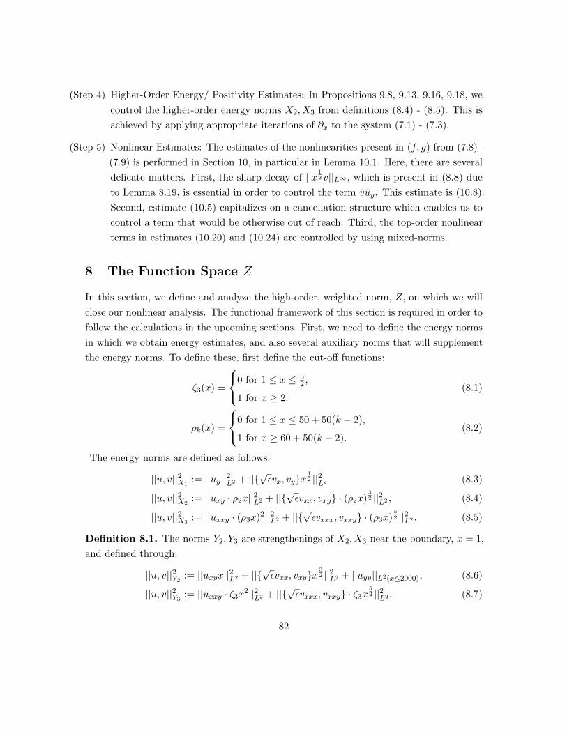
(Step 4) Higher-Order Energy/ Positivity Estimates: In Propositions 9.8, 9.13, 9.16, 9.18, we

control the higher-order energy norms X2, X3 from definitions (8.4) - (8.5). This is

achieved by applying appropriate iterations of ∂x to the system (7.1) - (7.3).

(Step 5) Nonlinear Estimates: The estimates of the nonlinearities present in (f, g) from (7.8) -

(7.9) is performed in Section 10, in particular in Lemma 10.1. Here, there are several

delicate matters. First, the sharp decay of ||x12 v||L∞ , which is present in (8.8) due

to Lemma 8.19, is essential in order to control the term vuy. This estimate is (10.8).

Second, estimate (10.5) capitalizes on a cancellation structure which enables us to

control a term that would be otherwise out of reach. Third, the top-order nonlinear

terms in estimates (10.20) and (10.24) are controlled by using mixed-norms.

8 The Function Space Z

In this section, we define and analyze the high-order, weighted norm, Z, on which we will

close our nonlinear analysis. The functional framework of this section is required in order to

follow the calculations in the upcoming sections. First, we need to define the energy norms

in which we obtain energy estimates, and also several auxiliary norms that will supplement

the energy norms. To define these, first define the cut-off functions:

ζ3(x) =

0 for 1 ≤ x ≤ 32 ,

1 for x ≥ 2.(8.1)

ρk(x) =

0 for 1 ≤ x ≤ 50 + 50(k − 2),

1 for x ≥ 60 + 50(k − 2).(8.2)

The energy norms are defined as follows:

||u, v||2X1:= ||uy||2L2 + ||

√εvx, vyx

12 ||2L2 (8.3)

||u, v||2X2:= ||uxy · ρ2x||2L2 + ||

√εvxx, vxy · (ρ2x)

32 ||2L2 , (8.4)

||u, v||2X3:= ||uxxy · (ρ3x)2||2L2 + ||

√εvxxx, vxxy · (ρ3x)

52 ||2L2 . (8.5)

Definition 8.1. The norms Y2, Y3 are strengthenings of X2, X3 near the boundary, x = 1,

and defined through:

||u, v||2Y2 := ||uxyx||2L2 + ||√εvxx, vxyx

32 ||2L2 + ||uyy||L2(x≤2000), (8.6)

||u, v||2Y3 := ||uxxy · ζ3x2||2L2 + ||

√εvxxx, vxxy · ζ3x

52 ||2L2 . (8.7)

82

Definition 8.2. The norm Z is defined through:

||u, v||Z :=||u, v||X1∩X2∩X3 + εN2 ||u, v||Y2 + εN3 ||u, v||Y3 + εN4 ||ux14 ,√εvx

12 ||L∞

+ εN5 supx≥20||√εvxx

32 , uxx

54 ||L∞ + εN6 sup

x≥20||uyx

12 ||L2

y

+ εN7

[ ∫ ∞20

x4||√εvxx||2L∞y dx

] 12. (8.8)

Here, Ni, are some large numbers which will be specified in (8.103) - (8.105). They depend

only on universal constants. It will be understood that Ni are much larger than any of the

quantities Mi appearing in the forthcoming lemmas, and that n is much larger than any of

the Ni,Mi.

Now that the norms we will be working in have been specified, we will define corresponding

spaces. First, some basic notations:

Definition 8.3. For any open set U ⊂ Ω, the space C∞0 (U) denotes the space of smooth

functions with compact support in U . We will also use C∞0 (U) to denote the space of

smooth vector fields with compact support in U , which will be clear from context. The

space C∞0,D(U) denotes the space of smooth, divergence-free vector fields with compact

support in U . When the set U is clear from context, we shall suppress it.

Definition 8.4. Given any open set U ⊂ Ω, the space Z(U) is defined to be space of those

divergence-free vector fields which lie in the closure of C∞0,D(U) under the norm X1, such

that ||u, v||Z <∞.

Definition 8.5. Given any open set U ⊂ Ω, the space (X1 ∩X2 ∩X3)(U) is defined to be

space of those divergence-free vector fields which lie in the closure of C∞0,D(U) under the

norm X1, such that ||u, v||X1∩X2∩X3 <∞.

Due to the weights in the norm Z and the energy norms X1∩X2∩X3, there is no “H = W

Theorem” generically available, which would equate the density of smooth functions with

compact support with the class of functions satisfying ||u, v||Z < ∞. This is the reason

must specify that:

Z(U) ⊂ C∞0,D||·||X1 (U). (8.9)

We will first record the boundary behavior of Z(Ω)-vector fields:

83

Lemma 8.6. For [u, v] ∈ Z(Ω), the following boundary conditions are satisfied:

[u, v]|x=1 = [u, v]|y=0 = limx→∞

[u, v] = limy→∞

[u, v] = 0. (8.10)

Proof. The boundary conditions at x = 1 and y = 0 are satisfied by the density specification

(8.9). The boundary conditions as x → ∞ is satisfied by the definition of norm Z, (8.8)

because the decay is encoded (with rates) in the norm. The boundary conditions as y →∞is enforced because [u, v] ∈ Z(Ω) implies that [u, v] ∈ H1

(x≤A), and candidacy in such a

Sobolev space automatically encodes decay as y →∞.

The above lemma shows that Z(Ω) is a suitable space to obtain solutions to our boundary-

value problem, after a consultation with (7.4). That X1∩X2∩X3 also encodes the boundary

conditions from (8.10) is less obvious, and is proven in Lemma 8.18.

Lemma 8.7. For any open set U ⊂ Ω, Z(U) and (X1 ∩X2 ∩X3)(U) are Banach spaces.

Proof. This follows from standard arguments.

For the energy norm, X1∩X2∩X3, we have Hilbertian structure. Given two divergence-free

vector-fields:

u := (u, v), a := (a, b), (8.11)

define the following inner-products:

〈u,a〉X1 :=

∫ ∫uyay +

∫ ∫uxaxx+

∫ ∫εvxbxx, (8.12)

〈u,a〉X2 :=

∫ ∫uxyaxy(ρ2x)2 +

∫ ∫uxxaxx(ρ2x)3 +

∫ ∫εvxxbxx(ρ2x)3, (8.13)

〈u,a〉X3 :=

∫ ∫uxxyaxxy(ρ3x)4 +

∫ ∫uxxxaxxx(ρ3x)5 +

∫ ∫εvxxxbxxx(ρ3x)5, (8.14)

〈u,a〉X1∩X2∩X3 := 〈u,a〉X1 + 〈u,a〉X2 + 〈u,a〉X3 . (8.15)

Temporarily accepting Lemma 8.18, we have:

Lemma 8.8. With the inner product (8.15), (X1 ∩X2 ∩X3)(Ω) is a Hilbert space.

Proof. The inner-product (8.15) is non-degenerate due to the boundary conditions [u, v]|y=0.

The remaining inner-product axioms are straightforward to check, which coupled with the

completeness in Lemma 8.7 gives the result.

84

Notationally, it sometimes is convenient to refer at once to all of the “uniform-type”

quantities in the norm Z, so we designate the following notation:

Definition 8.9. The norm U is defined by:

||u, v||U := εN4 ||ux14 ,√εvx

12 ||L∞ + εN5 sup

x≥20||√εvxx

32 , uxx

54 ||L∞

+ εN6 supx≥20||uyx

12 ||L2

y+ εN7

[ ∫ ∞20

x4||√εvxx||2L∞y dx

] 12. (8.16)

8.1 Elliptic Estimates and the Spaces Yi

We will first utilize elliptic theory in order to obtain basic Hk estimates for our solution,

which hold generically for Stokes-type equations. These elliptic estimates are meant to

supplement the energy estimates that we will perform in Section 9 which are meant to

control the energy norms, X1 ∩ X2 ∩ X3. In particular, the estimates from this section

cannot replace the energy estimates for two reasons:

(1) They scale poorly in ε, and

(2) One cannot extract sharp enough global-in-x information using this procedure.

Their purpose is to provide more controls near the boundary x = 1, which is reflected in

the norms Y2, Y3. To see this one should compare the support of the cut-off functions in our

energy norms, ρk, with the support of ζ3 in Y3. For the set of calculations in this subsection,

there are many different cutoff functions which arise in addition to the important cutoffs,

ρk, ζk which have already been defined.

Remark 8.10 (Notational Convention). To simplify notations, given a cut-off function χ,

we introduce the notation o(χ) to mean either χ or any of its derivatives, or any positive

powers of χ or any of its derivatives. Roughly speaking, any “variant” of χ is denoted by

o(χ), the essential feature being o(χ) is supported in the same (or similar) region.

The first step will be to provide some controls of ||u, v||H2 .

Lemma 8.11 (H2 Regularity). Let [u, v], [u, v] ∈ X1 be solutions to (7.1) - (7.3), with f, g

as in (7.8) - (7.9). For some M2, perhaps large, dependent only on universal constants:

supx≤2000

||u, v||L∞y + ||u, v||H2(x≤2000)

. ε−M2

[C + ε

n2

+γ ||u, v||L∞(||u, v||X1 + ||u, v||X1

)+ ||u, v||X1

]. (8.17)

85

Proof. Notationally, we will not take care to rename generic constants M2 within this proof.

We rescale the system back to Eulerian coordinates via:

u(x, Y ) := u(x, y), v(x, Y ) :=√εv(x, y), P (x, Y ) =

1

εP (x, y), (8.18)

which, by rescaling (7.1) - (7.3), yields the Stokes-sytem, for some M2 perhaps large:

−∆u+ Px = ε−M2

[f + Su

], −∆v + PY = ε−M2

[g + Sv

],

ux + vY = 0. (8.19)

Above, f , g, Su, Sv have been also rescaled to Eulerian coordinates. By considering the

stream function ψ =∫ Y

0 u, we obtain the following biharmonic problem:

∆2ψ = F := ε−M2∂Y[f + Su

]− ∂x

[g + Sv

], (8.20)

ψ(x, 0) = ψY (x, 0) = 0, ψ(1, Y ) = ψx(1, Y ) = 0. (8.21)

We now introduce the partition of unity, χmm≥1 of the region [1, 2000]× [0,∞). The

specifications of these cut-off functions are as follows. First, define:

χ(a)(x) =

1 for 1 ≤ x ≤ 2000,

0 for x ≥ 4000,χ(b)m (Y ) =

1 for m− 1 ≤ Y ≤ m+ 1,

0 for Y ≥ m+ 2,

0 for Y ≤ m− 2.

(8.22)

for all m ≥ 1. Then define:

χm(x, Y ) = χ(a)(x)χ(b)m (Y ). (8.23)

The purpose of selecting such a partition is to localize near x = 1, in such a way that the

region between 1 and the support of ρ2 is captured (see the definition in (8.2)). Denote by

ψm = χmψ Then:

∆2ψm = χmF + [∆2, χm]ψ, ψm(x, 0) = ∂Y ψm(x, 0) = ψm(1, Y ) = ∂xψm(1, Y ) = 0.

(8.24)

Here the commutator is defined as:

[∆2, χ]ψ :=χY Y Y Y ψ + 6χY Y ψY Y + 4χY Y Y ψY + 4χY ψY Y Y + 6χxxψxx + 4χxxxψx

+ 4χxψxxx + χxxxxψ + χxxY Y ψ + 2χY Y ψxx + 2χY Y xψx + 2χxψxY Y

86

+ 2χxxY ψy + 2χyψxxY + 4χxY ψxY . (8.25)

According to [BR80], Theorems 1 and 2, with k = 1, coupled with Figure 2, P. 562 in

[BR80] with “C/C” boundary conditions, we have the following H3 estimate for ψ:

||ψm||H3 . ||χmF ||H−1 + ||[∆2, χm]ψ||H−1 . (8.26)

We will first address the commutator terms in (8.26). First, consider the terms in (8.25)

which have three derivatives on ψ, which are denoted by o(∂3ψ). Using the definition of

H−1, for any compactly supported test function α(x, Y ) ∈ H10 ,∣∣∣〈o(χm)o(∂3ψ),α(x, y)〉H−1,H1

0

∣∣∣ =∣∣∣〈o(∂χm)o(∂2ψ), α〉

∣∣∣+∣∣∣〈o(χm)o(∂2ψ), ∂α〉

∣∣∣≤ ||o(χm)o(∂2ψ)||L2 ||α||H1

0. (8.27)

Then taking the sup over all ||α||H10

= 1, we obtain:

||o(χm)o(∂3ψ)||H−1 . ||o(χm)o(∂2ψ)||L2 . ||o(χm)o(∂)[u, v]||L2 . ε−M2 ||o(χm)]u, v||X1 .

(8.28)

Next, turn to the terms in (8.25) which has two derivatives on ψ:

||o(χm)o(∂2ψ)||H−1 ≤ ||o(χm)o(∂2ψ)||L2 ≤ ε−M2 ||o(χm)]u, v||X1 . (8.29)

Next, we must address those terms in (8.25) which has one derivatives on ψ. For this, we

use the Poincare inequality in x direction:

||o(χm)∂ψ||H−1 ≤ ||o(χm)∂ψ||L2 ≤ ||o(χm)u, v||L2 ≤ ||ux, vx||L2(x≤2000)

≤ ||o(χm)ux, vx||L2 ≤ ε−M2 ||o(χm)u, v||X1 . (8.30)

For the zeroeth order terms in ψ, we must argue as follows:

||o(χm)ψ||H−1 . ||o(χm)ψ||L2 = ||o(χm)

∫ x

0v||L2 . ||o(χm)

1

x

∫ x

0v||L2

. ε−1||o(χm)u, v||X1 . (8.31)

Summarizing, then,

||[∆2, χm]ψ||H−1 . ε−M2 ||o(χm)u, v||X1 , (8.32)

87

It remains, then, to analyze the majorizing terms in F in estimate (8.26). Up to redefining

M2 in (8.20), we may scale back to Prandtl coordinates (x, y). By integrating by parts

against compactly supported test functions, we have:

||χm · [∂y(f + Su)− ∂x(g + Sv)]||H−1 . ||o(χm)[f + Su + g + Sv

]||L2 . (8.33)

First, we’ll start with:

||o(χm) · Su||L2 = ||o(χm)[uRux + uRxu+ vRuy + uRyv

]||L2

≤ ||uR, xuRx, vR, uPRyy, uERY x32 ||L∞ ||o(χm)ux, uy, vy, vx||L2

. ||o(χm)u, v||X1 . (8.34)

Similarly,

||o(χm) · Sv||L2 = ||o(χm)[uRvx + vRxu+ vRvy + vRyv

]||L2 (8.35)

≤ ||uR, xvRx, vR, vRyy||L∞ ||o(χm)vx, ux, vy||L2 . ||o(χm)u, v||X1 .

Next, we come to the nonlinear terms:

εn2

+γ ||o(χm) ·[uux + vuy + uvx + vvy

]||L2

≤ εn2

+γ ||o(χm)u, v||L∞ ||o(χm)ux, vx, uy||L2

. εn2

+γ ||o(χm)u, v||L∞(||o(χm)u, v||X1 + ||o(χm)u, v||X1

). (8.36)

Finally, we have the forcing terms in f, g for which we cite Lemma 6.27,

∞∑m=1

||o(χm)Ru,n, Rv,n||L2 ≤ C. (8.37)

Upon taking summation in m:

||ψ||H3(x≤2000) ≤ ||∑m

χmψ||H3 ≤∑m

||χmψ||H3 ≤∑m

||χmF ||H−1 +∑m

||[∆2, χm]ψ||H−1

. ε−M2

[∑m

||o(χm)Ru,n, Rv,n||L2 +∑m

||o(χm)u, v||X1

+ εn2

+γ ||o(χm)||u, v||L∞(||o(χm)u, v||X1 + ||o(χm)u, v||X1

)]. ε−M2

[C + ||u, v||X1 + ε

n2

+γ ||u, v||L∞(||u, v||X1 + ||u, v||X1

)].

For the L∞ component of our desired claim, we simply use the standard H2 embedding.

88

Corollary 8.12. Suppose ||u, v||Z ≤ 1. There exists a universal constant M2 such that for

any selection of N2, N4, n, γ, the following estimate holds:

εN2 ||u, v||Y2 . εN2−M2 + εn2

+γ+N2−M2−N4 ||u, v||2Z

+(εN2−M2 + ε

n2

+γ+N2−M2−N4

)||u, v||X1 + εN2 ||u, v||X2 . (8.38)

We will now bootstrap the above elliptic regularity, away from the boundary x = 1 (thereby

avoiding the corners of our domain).

Lemma 8.13 (Third-Order Elliptic Regularity). For some M3 ≥ 0 perhaps large, but

independent of n, and supposing ||u, v||Z ≤ 1, we have:

||ux,√εvx · ζ3||H2(x≤1000) . ε−M3

[C + ||u, v||X1∩Y2 + ε

n2

+γ−N4−N2 ||u, v||X1∩Y2

]+ ε−M3−2N2−2N4+n

2+γ ||u, v||2Z . (8.39)

Proof. Start with the system in (8.20), and differentiate once in x:

∆2ψx = Fx := ε−M2∂Y[fx + ∂xSu

]− ∂x

[gx + ∂xSv

],

∂xψ(x, 0) = ∂xψY (x, 0) = 0. (8.40)

We shall now define a new cut-off function, via:

χ(2,a)(x) =

0 for 1 ≤ x ≤ 3

2 ,

1 for 2 ≤ x ≤ 1000,

0 for 2000 ≤ x.

(8.41)

Then, referring back to (8.22),

χ(2)m (x, Y ) := χ(2,a)(x)χ(b)

m (Y ) (8.42)

The collection χ(2)m is meant to fill the gap between ζ3 and ρ3 (see the definitions in

(8.1), (8.2)). We will consider the unknown χ(2)m ψx, which satisfies the system:

∆2(χ(2)m ψx

)= χ(2)

m Fx + [∆2, χ(2)m ]ψx, (8.43)

where the commutator expression is given by (8.25). Then via the standard, local in x,

H3 estimate, one has:

||χ(2)m ψx||H3 . ||χ(2)

m Fx||H−1 + ||[∆2, χ(2)m ]ψx||H−1 . (8.44)

89

Again, as [∆2, χ(2)m ] is localized in x and contains three-derivatives of ψx, we easily obtain:

||[∆2, χ(2)m ]ψx||H−1 . ε−M3 ||o(χ(2)

m )u, v||Y2∩X1 . (8.45)

We will now evaluate the Fx term above. By selecting the exponent M3 large enough, one

can rescale fx, gx to fx, gx and ∂xSu, ∂xSv to Su, Sv, which we automatically do. Then,

||χ(2)m Fx||H−1 ≤ ε−M3

[||χ(2)

m fxy||H−1 + ||χ(2)m gxx||H−1

]≤ ε−M3

[||o(χ(2)

m )fx||L2 + ||o(χ(2)m )gx||L2

]. (8.46)

Then, according to the definition (7.8) - (7.9), one has for the nonlinear terms:

||o(χ(2)m ) · N u

x ||L2 = εn2

+γ ||o(χ(2)m )[uuxx + u2

x + vxuy + vuxy]||L2

≤ εn2

+γ[||o(χ(2)

m )u||L∞ ||o(χ(2)m )uxx||L2 + ||o(χ(2)

m )ux||2L4

+ ||o(χ(2)m )vx||L4 ||o(χ(2)

m )uy||L4 + ||o(χ(2)m )v||L∞ ||o(χ(2)

m )uxy||L2

]≤ ε

n2

+γ[||o(χ(2)

m )u||L∞ ||o(χ(2)m )uxx||L2 + ||o(χ(2)

m )ux||L2 ||o(χ(2)m )ux||H1

+ ||o(χ(2)m )vx||

12

L2 ||o(χ(2)m )vx||

12

H1||o(χ(2)

m )uy||12

L2 ||o(χ(2)m )uy||

12

H1

+ ||o(χ(2)m )v||L∞ ||o(χ(2)

m )uxy||L2

]. ε

n2

+γ[ε−2N2−2N4 ||o(χ(2)

m )u, v||2Z + ε−2N2−2N4 ||o(χ(2)m )u, v||X1∩Y2

].

(8.47)

Above, we have used the assumption that ||u, v||Z ≤ 1 in the term:

||o(χ(2)m )vx||

12

L2 ||o(χ(2)m )vx||

12

H1||o(χ(2)

m )uy||12

L2 ||o(χ(2)m )uy||

12

H1

≤ ε−N2 ||v||Z ||o(χ(2)m )uy||

12

L2 ||o(χ(2)m )uy||

12

H1

≤ ε−N2 ||o(χ(2)m )uy||

12

L2 ||o(χ(2)m )uy||

12

H1

≤ ε−N2 ||o(χ(2)m )uy||

12X1ε−N2 ||o(χ(2)

m )u||12Y2. (8.48)

In the final estimate, we have used that χ(2) is supported on a strictly smaller region in x

than the region over which we have controlled uyy (compare (8.23) to the uyy estimate in

(8.17)). Similarly,

||o(χ(2)m )N v

x ||L2 = εn2

+γ ||o(χ(2)m )[uvxx + uxvx + vxvy + vvxy]||L2

90

≤ εn2

+γ[||o(χ(2)

m )u||L∞ ||o(χ(2)m )vxx||L2 + ||o(χ(2)

m )ux||L4 ||o(χ(2)m )vx||L4

+ ||o(χ(2)m )vx||L4 ||o(χ(2)

m )vy||L4 + ||o(χ(2)m )v||L∞ ||o(χ(2)

m )vxy||L2

]≤ ε

n2

+γ[ε−2N2−2N4 ||o(χ(2)

m )u, v||2Z]. (8.49)

Next, according to estimates (6.177), one has:∑m≥1

||o(χ(2)m )Ru,nx , o(χ(2)

m )Rv,nx ||L2 ≤ C. (8.50)

Taking summation in m and scaling back to Prandtl coordinates gives the desired result

upon comparing the supports of χ2 and ρ2:

||χ(2)ψ||H3 ≤∑m

||χ(2)m ψ||H3

. ε−M3∑m

||o(χ(2)m )u, v||Y2∩X1 + ε

n2

+γ∑m

ε−2N2−2N4 ||o(χ(2)m )u, v||2Z

+ εn2

+γε−N2−N4∑m

||o(χ(2)m )u, v||X1∩Y2 +

∑m

||o(χ(2)m )Ru,nx , o(χ(2)

m )Rv,nx ||L2

. ε−M3

[C + ||u, v||Y2∩X1 + ε

n2

+γ−2N2−2N4 ||u, v||2Z + εn2

+γ−N2−N4 ||u, v||X1∩Y2

].

(8.51)

Corollary 8.14. There exists a universal constant M3 such that for any selection of

N2, N3, N4, n, γ, so long as ||u, v||Z ≤ 1, we have:

εN3 ||u, v||Y3 . εN3−M3

[C + ||u, v||X1∩Y2

]+ εN3 ||u, v||X3

+ εn2

+γ−N2−N4−M3+N3 ||u, v||X1∩Y2 + εN3−M3−2N2−2N4+n2

+γ ||u, v||2Z . (8.52)

We now upgrade the previous estimate to a fourth order, weighted estimate. This fourth

order estimate is not included in our norm, (8.8). This will simply be used in order to

justify rigorously one of the integrations by parts in the energy estimates (in particular,

calculation (9.95)). This is the reason our right-hand side below in (8.53) need not be

depicted explicitly; we only need the qualitative information that this quantity is finite.

Lemma 8.15 (Fourth-Order Elliptic Regularity). Suppose ||u, v||Z ≤ 1. Solutions [u, v, P ] ∈Z to the system (7.1) - (7.3), with forcing terms as in (7.8) - (7.9) satisfy the following

fourth-order estimate:

||uxx,√εvxx · x||H2(x≥20) <∞. (8.53)

91

Proof. Taking two derivatives of (8.20), one has ∆2(ψxx) = Fxx. Define a partition of unity

of x ≥ 20, χmm≥0, such that χ0 is supported on Y ≥ 1, and all of the χm,m ≥ 1 are

localized near the boundary Y = 0 in the region Y ∈ [0, 2] and near x = m. Then:

∆2(χmxψxx) = [∆2, χmx]ψxx + xχmFxx, (8.54)

∆2(χ0xψxx) = [∆2, χ0x]ψxx + xχ0Fxx, (8.55)

where we refer the reader to the commutator expression in (8.25). For equation (8.55),

one uses the standard, interior H3 estimate for the Bi-Laplacian:

||χ0xψxx||H3 . ||[∆2, χ0x]ψxx||H−1 + ||xχ0Fxx||H−1 . (8.56)

For equation (8.54), one uses the boundary H3 estimate which gives:

||χmxψxx||H3 . ||[∆2, χmx]ψxx||H−1 + ||xχmFxx||H−1 . (8.57)

Let us write the expression for Fxx that we will read from, referring to (8.20) (we will

rename the power of ε)

Fxx = ε−M4

[∂xxY f + ∂xxY Su − ∂xxxg − ∂xxxSv

]. (8.58)

As usual, by sacrificing powers of ε, it suffices to evaluate the H−1 norm of the above

expression in Prandtl coordinates. We will start with Su:

||χm, χ0x∂xxY Su||H−1 . ||χm, χ0x∂xxSu||L2 + ||o(∂yχm, ∂yχ0)x∂xxSu||L2 . (8.59)

Similarly for Sv, one obtains:

||o(χm, χ0)∂xxxxSv||H−1 ≤ ||o(χm, χ0)∂xxSv||L2 + ||o(∂xχm, ∂xχ0)∂xxxSv||L2

+ ||o(χm, χ0)x∂xxSv||L2 . (8.60)

Computing two derivatives of Su, Sv, one obtains:

∂xxSu = uRxxxu+ 2uRxxux + uRxuxx + uRxxux + 2uRxuxx

+ uRuxxx + uRyxxv + 2uRyxvx + uRyvxx + vRxxuy + 2vRxuxy + vRuxxy, (8.61)

∂xxSv = uRxxvx + 2uRxvxx + uRvxxx + vRxxxu+ 2vRxxux

+ vRxuxx + vRxxvy + 2vRxvxy + vRvxxy + vRxxyv + 2vRxyvx + vRyvxx. (8.62)

92

From here, given χ0, χm are supported on x ≥ 20, it is easy to see that:

||o(χm, χ0)[x∂xxSu, x∂xxSv

]||L2(x≥20) . ||o(χm, χ0)u, v||Z . (8.63)

Next, turning to the expressions in f, g:

fxx = ε−n2−γRu,nxx + uuxxx + 3uxuxx + vxxuy + 2vxuxy + vuxxy, (8.64)

gxx = ε−n2−γRv,nxx + uxxvx + uvxxx + 2uxvxx + vxxvy + vvxxy + 2vxvxy. (8.65)

From here, using (6.177), and the definition the norm Z in (8.8), one observes:

||o(χm, χ0)[x∂xxf, x∂xxg

]||L2(x≥20) . ||o(χm, χ0)u, v||2Z + ||o(χm, χ0)u, v||2Z . (8.66)

Summarizing this:∑m≥0

||xχmFxx||H−1 .∑m≥0

||o(χm)u, v||Z +∑m≥0

||o(χm)u, v||2Z

+∑m≥0

||o(χm)u, v||Z <∞. (8.67)

We now move to the commutator terms from (8.56) - (8.57), which we write out, denoting

by χ generically either χm or χ0:

[∆2, xχ]vx = ∂xyy(xχ)vxx + ∂xxy(xχ)vxy + ∂x(xχ)∂xyyvx + x∂yyχvxxx

+ ∂y(xχ)∂xxyvx + ∂xx(xχ)vxyy + ∂xy(xχ)vxxy

+4∑

k=1

∂kx(xχ)∂4−kx vx +

4∑k=1

x∂kyχ∂4−ky vx. (8.68)

Examining the commutator terms, one observes that the worst term is when all derivatives

fall on the cut-off, and none on either x or vx. Such a term arises, for instance, when k = 4

in the final summation above in (8.68). In this case, one uses that the partition of unity is

selected such that ∂yχ0, χm is a bounded region in y:

||∂4yχm, χ0 · xvx||H−1 ≤ ||∂4

yχm, χ0 · xvx||L2 . ||o(χm), o(∂χ0)xvxy||L2 . (8.69)

It is straightforward to check that all terms in the commutator can be estimated either in

this manner or directly using the definitions of Z in (8.8). Thus, taking summation over

the partition of unity again gives:∑m≥0

||[∆2, χmx]ψxx||H−1 . ||u, v||Z <∞. (8.70)

Combining (8.56), (8.57), (8.67), and (8.70), the lemma is proven.

93

8.2 Embedding Theorems for the Space Z

The next task is to pinpoint the interplay between the uniform quantities in the norm Z

and the norms Yi. Let us start with:

Lemma 8.16. For σ > 0 arbitrarily small,

supx≥1

[||√εψx−1−σ||2L2

y+ ||ux−σ||2L2

y+ ||√εvx−σ||2L2

y

]. C(σ)||u, v||2X1

, (8.71)

supx≥1

[||uyx

12 ||2L2

y+ ||uxx||2L2

y

]+ supx≥20||√εvxx||2L2

y. ||u, v||2X1∩Y2 , (8.72)

supx≥20

[||uxyx

32 ||2L2

y+ ||vxy,

√εvxxx2||2L2

y

]. ||u, v||2Y2∩Y3 . (8.73)

The constant C(σ) ↑ ∞ as σ ↓ 0. Finally, for [u, v] ∈ Z, we have the following property:

supx≥20||vxxx, uxxyx||L2

y<∞, (8.74)

Remark 8.17. The estimate (8.74) is required in order to rigorously justify one integration

by parts in our energy estimates, in particular calculation (9.100), and is not required as

part of the norm Z, which is why we do not characterize the right-hand side. The most

important parts of this lemma are the first three estimates, (8.71) - (8.73).

Proof. First, take a differentiation of:

∂x

∫u2x−2σ dy = 2

∫uuxx

−2σ dy − 2σ

∫u2x−1−2σ dy, (8.75)

which upon an integration in x, and recalling u(1, y) = 0, yields:∫u2x−2σ

1 dy = 2

∫ x1

1

∫uuxx

−2σ dx dy − 2σ

∫ x1

1

∫u2x−1−2σ dx dy. (8.76)

Taking absolute values, applying Holder’s inequality, and taking the supremum in x1:

supx≥1

∫u2x−2σ . ||ux−σ−

12 ||L2 ||uxx

12 ||L2 + ||ux−

12−σ||2L2 . ||uxx

12 ||2L2 . ||u, v||2X1

. (8.77)

Here the factor of σ > 0 is required to avert the critical Hardy inequality, which occurs

with weight x−12 in L2. The stream function estimate follows similarly:

∂x

∫ψ2x−2−σ = 2

∫ψvx−2−σ − (2− σ)

∫ψ2x−3−σ,

94

and so integration gives:

supx≥1

∫ψ2x−2−σ ≤ ||ψvx−2−σ||L1 + ||ψx−

32−σ

2 ||2L2 . ||vx−12−σ

2 ||2L2 . ||vxx12−σ

2 ||2L2

. ||u, v||2X1. (8.78)

The estimate for v in (8.71) works in a similar fashion. We will now move to first-order

estimates in (8.72). The uy estimate follows easily after a differentiation:

∂x

∫u2yx = 2

∫uyuxyx+

∫u2y. (8.79)

Taking an integration in x, and recalling that uy(1, y) = 0, then gives:

supx≥1

∫u2yx . ||uy||L2 ||uxyx||L2 + ||uy||2L2 . ||u, v||2X1∩Y2 . (8.80)

Next,

∂x

∫u2xx

2 = 2

∫uxuxxx

2 + 2

∫u2xx, (8.81)

so taking an x-integration and using that ux(1, y) = 0, we have:

supx≥1

∫u2xx

2 . ||uxx12 ||L2 ||uxxx

32 ||L2 + ||uxx

12 ||2L2 . ||u||2X1∩Y2 .

Let us now introduce new cut-off functions, for k = 2, 3:

ηk(x) =

0 for 1 ≤ x ≤ 3 + 6(k − 2),

1 for x ≥ 6 + 6(k − 2).(8.82)

Then η2, η3 are “in-between” ζ3 and ρ2, ρ3. Consider now the quantity∫εv2xx

2η2(x):

∂x

∫εv2xx

2η2(x) = 2

∫εv2xxη2(x) + 2

∫εvxvxxx

2η2 +

∫εv2xx

2η′2(x). (8.83)

As η2 vanishes on [1, 3], we can take the integration up from x = 1:

supx≥20

∫εv2xx

2 ≤ supx≥1

∫εv2xx

2η2(x) . ||√εvxx

12 ||2L2 + ||

√εvxxx

32 ||2L2 , (8.84)

where we have used that |η′2(x)x2| . 1. We now move to the second-order estimates in

(8.73), starting with:

∂x

∫u2xyx

3η3 = 2

∫uxyuxxyx

3η3 +

∫u2xy3x

2η3 +

∫u2xyx

3η′3. (8.85)

95

Using that η3uxy(1, y) = 0, we have:

supx≥1

∫u2xyx

3η3 . ||uxyx||2L2 + ||uxyx||L2 ||uxxyx2η3||L2 . ||u, v||2Y2∩Y3 . (8.86)

Above, we have used that η3 ≤ ζ3. The final calculation is:

∂x

∫v2xyx

4η3 = C

∫vxyvxxyx

4η3 + C

∫v2xyx

3η3 + C

∫v2xyx

2η′3. (8.87)

Integrating up from x = 1,

supx≥1

∫v2xyx

4η3 . ||vxyx32 ||2L2 + ||vxxyx

52 η3||2L2 . ||u, v||2Y2∩Y3 . (8.88)

It is clear that√εvxx works in an identical manner to (8.87), and also in an identical

manner, one obtains (8.74) by pairing with (8.53).

We will now record the following about the x→∞ behavior of elements in (X1 ∩X2 ∩X3)(Ω):

Lemma 8.18. Suppose [u, v] ∈ X1 ∩X2 ∩X3(Ω). Then the following boundary conditions

are automatically enforced:

[u, v]|x=1 = [u, v]|y=0 = limx→∞

[u, v] = limy→∞

[u, v] = 0 (8.89)

Proof. All follow as in Lemma 8.6 aside from the condition at x→∞. For this, we use:

||ux14−σ||L∞y ≤ ||ux

−2σ||12

L2y||uyx

12 ||

12

L2y<∞, (8.90)

||vx12−σ||L∞y ≤ ||vx

−2σ||12

L2y||vyx||

12

L2y<∞, (8.91)

according to the estimates in (8.71). Thus, we can conclude that [u, v]→ 0 as x→∞.

The estimates (8.90) - (8.91) yield uniform decay of [u, v] as x→∞. However, the factor of

x−σ is too weak to close our nonlinear analysis (see estimate (10.8)). This in turn is caused

by Hardy’s inequality being critical (see (8.77)). In the next lemma, we use higher-order

decay estimates to avoid this criticality:

96

Lemma 8.19 (Uniform Embeddings). For [u, v] ∈ X1 ∩X2 ∩X3(Ω), we have:

supx≥1||ux

14 ,√εvx

12 ||L∞y . ||u, v||X1∩Y2∩Y3 , (8.92)

supx≥20||uxx

54 ,√εvxx

32 ||L∞y . ||u, v||X1∩Y2∩Y3 . (8.93)

Proof. We will first turn to the first-order estimates in (8.93). These follow from the

evolution estimates in the previous lemma via standard Sobolev interpolation:

||uxx54 ||L∞y ≤ ||uxx||

12

L2y||uxyx

32 ||

12

L2y. (8.94)

Similarly,

||vxx32 ||L∞y ≤ ||vxx||

12

L2y||vxyx2||

12

L2y. (8.95)

The result now follows after taking the supremum in x ≥ 20 and appealing to the evolution

estimates above. Next, we address (8.92). For x ≤ 20, we may simply appeal to the uniform

estimates in estimate (8.17). For v, the result follows immediately from:∣∣∣v(x, y)∣∣∣ =

∣∣∣ ∫ ∞x

vx(x′, y)dx′∣∣∣ ≤ ||vxx 3

2 ||L∞y∫ ∞x

(x′)−32dx′ =

[supx≥20||vxx

32 ||L∞y

]x−

12 . (8.96)

We have used the qualitative boundary condition that v → 0 as x→∞, which is available

due to Lemma 8.18. For the u estimate follows in the same manner:∣∣∣u(x, y)∣∣∣ ≤ ||uxx 5

4 ||L∞y∫ ∞x

(x′)−54dx′ .

[supx≥20||uxx

54 ||L∞y

]x−

14 . (8.97)

Now taking the sup in x, y of both of the above inequalities yields the desired result.

We now turn to controlling the top-order uniform-type norm:

Lemma 8.20 (Top Order Uniform Embedding). For [u, v] ∈ X1 ∩ Y2 ∩ Y3, one has the

following mixed-norm estimate:∫ ∞20

x4||√εvxx||2L∞y dx+

∫ ∞20

x72 ||uxx||2L∞y dx . ||u, v||2X1∩Y2∩Y3 . (8.98)

Proof. For x ≥ 20, we start with:

x2||√εvxx||L∞y ≤ ||x

32√εvxx||

12

L2y||x

52√εvxxy||

12

L2y.

97

Taking square on both sides:

x4||√εvx||2L∞y ≤ ||x

32√εvxx||2L2

y+ ||x

52√εvxxy||2L2

y, (8.99)

so integrating ∫ ∞20

x4||√εvxx||2L∞y dx ≤ ||u, v||

2X1∩Y2∩Y3 . (8.100)

For the uxx estimate, we have:

x74 ||uxx||L∞y ≤ ||x

32uxx||

12

L2y||x2uxxy||

12

L2y, (8.101)

Squaring both sides and taking an x-integration gives:∫ ∞20

x72 ||uxx||2L∞y ≤

∫ ∞20||x

32uxx||2L2

y+

∫ ∞20||x2uxxy||2L2

y

. ||u, v||2X1∩Y2∩Y3 . (8.102)

We shall make the following selections, given arbitrary constants M2,M3 ≥ 0:

N2 is selected such that N2 −M2 = 100; (8.103)

N3 is selected such that N3 −M3 = 2N2; (8.104)

Nk = N3 for k = 4, 5, 6, 7, (8.105)

n sufficiently large relative to Ni,Mi. (8.106)

We now consolidate the above series of lemmas, coupled with (8.38) and (8.52).

Corollary 8.21. With N4, ..., N7 as in (8.105), we have:

||u, v||U . εmaxN2,N3||u, v||X1∩Y2∩Y3 . (8.107)

Theorem 8.22 (Z embedding). Suppose ||u, v||Z ≤ 1. For appropriate choices of N2, ...N7,

based only on universal constants, there exists a universal constant ω(Ni) such that:

||u, v||Z . ε100 + ||u, v||X1∩X2∩X3 + εn2

+γ−ω(Ni)||u, v||2Z . (8.108)

98

Proof. According to (8.107), it suffices to treat the Y2, Y3 terms in || · ||Z . For this we simply

use the selections in (8.103) - (8.106) to rewrite (8.52)

εN3 ||u, v||Y3 . ε100 + ε100||u, v||X1∩X3 + εN2 ||u, v||Y2 + εn2

+γ−ω(Ni)||u, v||2Z . (8.109)

The condition (8.106) allows us to control, in estimate (8.52):

εn2

+γ−N2−N4−M3+N3 ||u, v||X1∩Y2 ≤ εN2+100||u, v||X1∩Y2 , (8.110)

for instance, so long as: n2 + γ −N2 −N4 −M3 +N3 > N2 + 100. There are many such

criteria which arise over the course of our analysis, and so we retain the generality as stated

in (8.106). Next, rewriting (8.38) in a similar fashion, one has:

εN2 ||u, v||Y2 . ε100 + ε100||u, v||X1∩X2 + εn2

+γ−ω(Ni)||u, v||2Z . (8.111)

Summing these two estimates yields the desired result.

8.3 Function Space, Z(ΩN)

We will have occasion to consider, Z(ΩN ), where ΩN is defined in (7.10), and N is some

large but finite, fixed number. Due to the boundedness in the y-direction of ΩN :

Lemma 8.23. For [u, v] ∈ Z(ΩN ),

||ψ||L2(ΩN ) + ||√εv, vyx||L2(ΩN ) ≤ C(N)||u, v||Z(ΩN ), (8.112)

where C(N) depends poorly on large N .

Proof. This follows from the Poincare inequality, as both ψ = v = vy = 0 on y = 0:

||vx||L2 ≤ C(N)||vyx||L2 ≤ C(N)||vyyx||L2 = ||uxyx||L2y. C(N)||u, v||Z(ΩN ). (8.113)

Similarly,

||ψ||L2 ≤ C(N)||ψy||L2 = ||u||L2 ≤ C(N)||uy||L2 ≤ C(N)||u||Z(ΩN ). (8.114)

99

Lemma 8.24. For [u, v] ∈ Z(ΩN ),

supx≥20

[x

32 ||v, vy||L2

y+ x

12 ||ψ||L2

y+ x

12 ||u||L2

y+ x2||vx||L2

y

]≤ C(N)||u, v||Z(ΩN ), (8.115)

where C(N) depends poorly on large N .

Proof. By applying the Poincare inequality twice in the y-direction,

||vx32 ||L2

y≤ C(N)||vyx

32 ||L2

y≤ C(N)||uxyx

32 ||L2

y. ||u, v||Z . (8.116)

The final inequality following from (8.73). Similarly,

||vxx2||L2y≤ C(N)||vxyx2||L2

y. ||u, v||Z . (8.117)

Finally, by repeating all of the calculations which culminated in Theorem 8.22 on the

domain ΩN , the following estimate holds:

Theorem 8.25 (Z(ΩN ) embedding). Fix any N > 0, large. Suppose ||u, v||Z(ΩN ) ≤ 1. For

appropriate choices of N2, ...N7, based only on universal constants, there exists a universal

constant ω(Ni) such that we have:

||u, v||Z(ΩN ) . ε100 + ||u, v||X1∩X2∩X3(ΩN ) + εn2

+γ−ω(Ni)||u, v||2Z(ΩN ). (8.118)

The constants in the above estimate are independent of N .

9 Navier-Stokes Remainders: Energy Estimates

In this section, we shall obtain a family of energy and positivity estimates for the system

in (7.1) - (7.3). As mentioned in the prior section, we seek a solution [u, v] ∈ Z(Ω), where

Z(Ω) is defined precisely in equation (8.4). Our point of view for this section, then, is to

obtain a-priori estimates under the assumption that [u, v] ∈ Z. Such a solution necessarily

encodes decay rates of the solutions and their derivatives (see, for instance, (8.71) - (8.73),

(8.92), and (8.93)). We shall give a-priori estimates on the domain ΩN , as defined in (7.10),

which are independent of N , allowing us to take N →∞. For this purpose, we take the

boundary conditions shown in (7.11).

Remark 9.1 (Notational Convention). For Section 9, all integrations∫ ∫

and norms, || · ||,without further specification of domains are over ΩN .

100

Going to the vorticity formulation of (7.1) - (7.3):

∂y

(−∆εu+ Px + Su

)− ε∂x

(−∆εv +

Pyε

+ Sv

)=

∂y

(−∆εu+ Su

)− ε∂x

(−∆εv + Sv

)= fy − εgx. (9.1)

Define the stream function through

ψ(x, y) = −∫ y

0u(x, y′)dy′, ψx = v, ψy = −u, (9.2)

and note via the boundary conditions (7.4) and (7.11),

ψ|y=0,y=N = ψ|x=1 = ψx|x=1 = ψy|y=0,y=N = 0. (9.3)

To see that ψ|y=N = 0, we can write:

∂xψ = −∫ N

0ux(x, y′)dy′ =

∫ N

0vy(x, y

′)dy′ = v(x,N)− v(x, 0) = 0. (9.4)

Next, the boundary condition ψ(1, y) = 0 enables us to evaluate ψ the corner: ψ(1, N) = 0.

Thus, coupling these two facts yields ψ(x,N) = 0. Next, we record the observation:

ψ(x, y) = ψ(x, y)− ψ(1, y) =

∫ x

1∂xψ(x′, y)dx′ =

∫ x

1v(x′, y)dx′, (9.5)

and so taking absolute values, and supremum in y yields:

||ψ(x′)||L∞y ≤∫ x

1||v(x′)||L∞y dx

′ ≤∫ x

1(x′)−

12dx′ . x

12 . (9.6)

We also will have occassional need for the auxiliary domain:

ΩNM := 0 < x < M, 0 < y < N. (9.7)

9.1 Energy Estimates

We now give the energy estimates on [u, v]. Let us first introduce the notation:

W1,E = |∫ ∫

f · u|+∫ ∫

ε|g||v|, (9.8)

W1,P =

∫ ∫|f ||vy|x+

∫ ∫ε|g||vx|x, (9.9)

W1 =W1,E +W1,P . (9.10)

101

Proposition 9.2. Let ε << δ and δ, ε be sufficiently small relative to universal constants.

Let [u, v] ∈ Z(ΩN ) be solutions to the system (7.1) - (7.3) on the domain ΩN . Then these

solutions satisfy the a-priori energy estimate:

||√εux, uy||2L2 ≤ O(δ)||

√εvxx

14 , vyx

12 ||2L2 +W1,E . (9.11)

The constant in the above estimate is independent of N .

Remark 9.3. Note carefully in (9.8) that we do not bring the absolute value inside of the

integration for the∫ ∫

fu term, which is important to treat term (10.5). For the remaining

terms above in W1, we place the absolute values inside the integration for convenience (in

terms of comparison with other terms that arise, see for instance (9.160) - (9.161)).

Proof. The vorticity equation (9.1) is multiplied by the stream function ψ and we proceed

to integrate by parts. According to the definition of the norm Z in (8.8) and the estimate

(8.112), all integrands appearing in this estimate will be L1(ΩN ), and so all applications of

Fubini are justified. First, we will treat the highest order terms:∫ ∫∂y

(−∆εu

)ψ + ε∂x∆εvψ =

∫ ∫∆εuψy − ε∆εvψx (9.12)

= −∫ ∫

∆εuu− ε∫ ∫

∆εvv (9.13)

=

∫ ∫|∇εu|2 + ε

∫ ∫|∇εv|2 − lim

M→∞

[ ∫x=M

εuxu+ ε2vxv]

(9.14)

=

∫ ∫|∇εu|2 + ε

∫ ∫|∇εv|2. (9.15)

For the limiting integrals over x = M above, we have used the bounds from (8.112) to

conclude:

|∫x=M

εuux| ≤ ε||ux12 ||L2

y||uxx

32 ||L2

yM−2 M→∞−−−−→ 0, (9.16)

|∫x=M

ε2vvx| ≤ ε2||vx32 ||L2

y||vxx2||L2

yM−

72M→∞−−−−→ 0. (9.17)

Let us justify rigorously the integration by parts found in line (9.12). To isolate the corners,

define C1,2r to be solid balls of radius r centered at the two corners, (1, 0), and (1, N). Then,∫ ∫∂y

(−∆εu

)ψ =

∫ ∫ΩN−∪2i=1C

ir

∂y

(−∆εu

)ψ +

2∑i=1

∫ ∫Cir

∂y

(−∆εu

)ψ (9.18)

102

=

∫ ∫ΩN−∪2i=1C

ir

−∆εuu−∫∂Cir

∆εuψdS +

∫ ∫Cir

∂y

(−∆εu

)ψ. (9.19)

First, as we know −∆εuu ∈ L1(ΩN ), we have:

limr→0

∫ ∫ΩN−∪2i=1C

ir

−∆εuu =

∫ ∫−∆εuu. (9.20)

Next, we appeal to the classical expansion in the vicinity of a corner point in [BR80], Page

57, equation (5.5), from which it follows that:

|u, v| . r, |ψ| . r, |∇2u,∇2v| . r−1 in Cir. (9.21)

Then the boundary integral from (9.19) can be controlled via:∣∣∣ ∫∂Cir

∆εuψ∣∣∣ ≤ ∫

∂Cir

∣∣∣∆εuψ∣∣∣ ≤ ∫

∂Cir

rr−1dS ≤ r r→0−−−→ 0. (9.22)

Finally, we arrive at the interior term from the corners in (9.19). For this, the expansion

in [BR80], Page 57, equation (5.5) implies that:

|∇3[u, v]|+ |∇3ψ| . r−2 + u, where u ∈ L2. (9.23)

Using this gives:∣∣∣ ∫ ∫Cir

∂y

(−∆εu

)ψdxdy

∣∣∣ . ∫ ∫Cir

∣∣∣r−2r∣∣∣dxdy +

∫ ∫Cir

|u|rdxdy

≤∫ ∫

Cir

r−2rrdrdω + ||u||L2(Cir)||r||L2(Cir)

r→0−−−→ 0. (9.24)

Summarizing, we have shown the validity of the integration by parts∫ ∫∂y(−∆εu)ψ =

∫ ∫−∆εuu. (9.25)

This calculation works generically at the corners (it was not specific to the particular

derivatives involved, just the order of them), and so we will avoid repeating it each time.

We now turn to the v-terms in (9.12), for which we write:∫ ∫ΩN−Cir

∂x∆εvψ = limM→∞

∫ ∫ΩNM−Cir

∂x∆εvψ

= − limM→∞

[ ∫ ∫ΩNM−Cir

∆εvv +

∫x=M

∆εvψdy −∫∂Cir

∆εvψdy]

103

= −∫ ∫

ΩN−Cir∆εvv + lim

M→∞

∫x=M

∆εvψdy −∫∂Cir

∆εvψdy. (9.26)

For the x = M boundary term in (9.26), we have:∣∣∣ ∫x=M

∆εvψ∣∣∣ ≤ ||∆εv||L2

y||ψ||L2

y. ||ψx

12 ||L2

y||∆εvx

32 ||L2

yM−2 M→∞−−−−→ 0, (9.27)

according to (8.71), (8.73), and (8.115). Subsequently, sending r → 0 as above gives the

desired identity: ∫ ∫∂x∆εvψ = −

∫ ∫∆εvv. (9.28)

Next, we come to the profile terms, Su, from the equation (7.1). We refer the reader to

the definition of Su, which is in (7.6).∫ ∫∂y

(Su

)ψ = −

∫ ∫Suψy =

∫ ∫Suu

=

∫ ∫ [uRux + uRxu+ vRuy + uRyv

]u. (9.29)

The first three of these terms in∫ ∫

Suu are handled through an integration by parts:∫ ∫uRuxu+ uRxu

2 + vRuuy =

∫ ∫uRxu

2 + limM→∞

∫x=M

uR2u2 = −

∫ ∫vRyu

2. (9.30)

Above, we have used the estimate for ||ux12 ||L2

yin (8.115). The term on the right-hand

side of (9.30) is handled via:∫ ∫vRyu

2 =

∫ ∫ (vPRy +

√εvERY

)u2

≤ ||vPRyy2||L∞ ||u

y||2L2 +

√ε||vERY x

32 ||L∞ ||

u

x34

||2L2

≤ O(δ)||uy||2L2 +O(δ)||uxx14 ||2L2 . (9.31)

In (9.31), we have first used the profile estimates in (2.10) and (2.20), and subsequently

the Hardy inequality which is available (for exponents of x which are not equal to 12) as

u(1, y) = u(x, 0) = 0. The large convective term in∫ ∫

Suu, (9.29), is given by:∫ ∫uRyuv =

∫ ∫uP,n−1

Ry + εn2 unp +

√εuERY uv. (9.32)

104

First, by estimate (2.14), with j = 1,m = 1, we have:

∣∣∣ ∫ ∫ uP,n−1Ry uv

∣∣∣ ≤ ||y2x−12uP,n−1

Ry ||L∞ ||u

y||L2 ||

vx12

y||L2 ≤ O(δ)||uy||L2 ||vyx

12 ||L2 . (9.33)

Second, according to (2.16) with j = 1:

∣∣∣ ∫ ∫ εn2 unpyuv

∣∣∣ ≤ εn2 ||unpyyx 12−σn ||L∞ ||ux−1+σn ||L2 ||

vx12

y||L2

≤ C(n)εn2 ||uxxσn ||L2 ||vyx

12 ||L2 . C(n)ε

n2 ||uxx

12 ||L2 ||vyx

12 ||L2 . (9.34)

Third, according to (2.18):∣∣∣ ∫ ∫ √εuERY uv∣∣∣ ≤ ||uERY x 32 ||L∞ ||

u

x34

||L2 ||√εv

x34

||L2

≤√ε||uxx

14 ||L2 ||

√εvxx

14 ||L2 . (9.35)

In (9.33), we have used the Hardy inequality in the y direction:

||vyx

12 ||L2 = ||||v

yx

12 ||L2

y||L2

x≤ ||vyx

12 ||L2 , (9.36)

which is available as v|y=0 = 0. We have also used the Hardy inequality in x direction,

which is available as v|x=1 = 0. Rigorously, turning to (9.34):

|| u

x1−σ ||L2 = |||| u

x1−σ ||L2x||L2

y≤ |||| u

(x− 1)1−σ ||L2x||L2

y. ||||ux(x− 1)σ||L2

x||L2

y(9.37)

. ||||uxxσ||L2x||L2

y= ||uxxσ||L2 . (9.38)

Summarizing, ∣∣∣ ∫ ∫ Suu∣∣∣ ≤ O(δ)||uy||2L2 +O(δ)||

√εvxx

14 , vyx

12 ||2L2 . (9.39)

The important mechanism in controlling (9.33) is the ability to trade a factor of y2x−12

which is absorbed by the Prandtl profiles, uP,n−1Ry , according to (2.16) with j = 1,m = 2.

This creates two y derivatives, uy and vyx12 , both of which are order 1. The next step is to

control the profile terms Sv:

− ε∫ ∫

∂xSvψ = ε

∫ ∫Svv − ε lim

M→∞

∫x=M

Svψ = ε

∫ ∫Svv. (9.40)

105

By inspecting (8.115), one sees easily that the above limit vanishes. We now treat the

interior terms from (9.40), which we expand for convenience:∫ ∫Svεv =

∫ ∫ (uRvx + vRxu+ vRvy + vRyv

)εv. (9.41)

The first, third, and fourth terms above in (9.41) are given via the following calculations:∫ ∫εuRvxv + εvRvvy + εvRyv

2 = ε

∫ ∫vRyv

2 + limM→∞

∫x=M

ε

2uRv

2

= ε

∫ ∫vRyv

2 (9.42)

≤ ε||vPRyy2||L∞ ||vy||2L2 +√ε||vERY x

32 ||L∞ ||

√εvxx

14 ||2L2 (9.43)

. ε||vy||2L2 +√ε||√εvxx

14 ||2L2 . (9.44)

The M−limit vanishes by the estimate for ||vx32 ||L2

yin (8.115). We have also used estimates

(2.10) and (2.17) for the profiles. Next,∣∣∣ ∫ ∫ εvRxuv∣∣∣ ≤ √ε||x 3

2 vRx||L∞ ||uxx14 ||L2 ||

√εvxx

14 ||L2 . (9.45)

Again, we have used (2.8) and (2.17) for the profiles. Thus,∣∣∣ ∫ ∫ Svεv∣∣∣ . √ε||√εvxx 1

4 , vyx14 ||2L2 . (9.46)

On the right-hand side of equation (9.1), we have:∫ ∫ (fy − εgx

)ψ = −

∫ ∫fψy +

∫ ∫εgψx =

∫ ∫fu+ εgv. (9.47)

First, we will note that each term in the above integration by parts is in L1(ΩN ), which

follows from the definitions in (7.5), and a consultation with the definition of Z in (8.8):

fy = ε−n2−γRu,ny + ε

n2

+γ(uyux + uuxy + vyuy + vuyy

), (9.48)

gx = ε−n2−γRv,nx + ε

n2

+γ(uxvx + uvxx + vxvy + vvxy

). (9.49)

It remains to justify the boundary terms resulting from the x-integration by parts, at

x → ∞, in (9.47). This, however, follows just as in (9.40) by inspecting the decay rates

in (8.115). A comparison with (9.8) then gives the desired result. Combining all of the

previous estimates proves (9.11).

106

9.2 Positivity Estimate

We now give the following Positivity estimate:

Proposition 9.4. Let ε << δ and δ, ε be sufficiently small relative to universal constants.

Then [u, v] ∈ Z(ΩN ) solutions to the system (7.1) - (7.3) satisfy the following estimate:

ε2∫x=1

v2x dy + lim

M→∞

∫x=M

u2yx dy + ||

(√εvx, vy

)x

12 ||2L2 . ||uy||2L2 +W1. (9.50)

Remark 9.5 (Selection of Multiplier). There is a distinction between the Positivity estimate

from [GN14], Page 31, and the present case. In the case of [GN14], the profiles, uR, were

not assumed small, and so they required the normalized multipliervyuR− ε vxuR . In our case

as the profiles are assumed size δ, we need not normalize by a factor of uR. On the other

hand, we need to capture precise behavior at x→∞, which is the reason our multiplier is

(vy − εvx) · x, or equivalently in the vorticity formulation, v · x.

Proof. We apply the multiplier xψx = xv to the equation (9.1), and we will subsequently

take the following integration:

limM→∞

∫ ∫ΩNM

Equation (9.1) · xv dy dx. (9.51)

The purpose of specifying the order of integration is for the terms in (9.54), which are not

automatically in L1(ΩN ) prior to integrating by parts in y. All other terms are in L1(ΩN )

according to the norm Z, (8.8), and the estimate (8.112). Thus, with the exception of the

term in (9.54), the limiting procedure above can (and will) be omitted, and Fubini can be

justified.

Second Order Terms

First, we will treat the highest order terms. Let us begin with:

−∫ ∫

∂y∆εuvx =

∫ ∫(εuxx + uyy)vyx. (9.52)

We will note that the uxx term on the right-hand side above is in L1(ΩN ), away from

the corners. This follows from the definition of Z, and (8.112). Thus, the forthcoming

applications of Fubini are justified:∫ ∫εuxxvyx = −

∫ ∫εvxyvyx = − ε

2

∫ ∫∂x

(v2y

)x

107

=ε

2

∫ ∫v2y − lim

M→∞

ε

2

∫x=M

v2yx =

ε

2

∫ ∫v2y . (9.53)

The above limit vanishes according to (8.115). For the uyy term in (9.52), we can integrate

by parts again in y, due to (9.51), to obtain:∫ ∫ΩNM

uyyvyx dy dx = −∫ ∫

ΩNM

uyvyyx dy dx. (9.54)

Now, the right-hand side of (9.54) is in L1(ΩN ) according to our norm Z. Interchanging

the order of integration:∫ ∫ΩNM

uyyvyx dy dx =

∫ ∫ΩNM

∂x

(u2y

2

)x dx dy = −

∫ ∫ΩNM

u2y

2dx dy +

∫x=M

u2y

2x. (9.55)

As the solid integrals on the right-hand side of (9.55) is known to be in L1(ΩN ), we can

pass to the limit M → ∞ (and also drop the notation dxdy when the order no longer

matters):

limM→∞

−∫ ∫

ΩNM

∂yuyy · vxdy dx = −∫ ∫

u2y

2+ limM→∞

∫x=M

u2yx. (9.56)

The limit above appears with a good sign, and therefore contributes to the left-hand

side of the desired estimate in (9.50). We have omitted the delicate limiting process near

the corners in this calculation, as this process is identical to that of (9.19). We shall now

examine the term:∫ ∫ε∂x∆εvvxdy dx =

∫ ∫ε(εvxxx + vxyy

)vxdy dx (9.57)

A direct computation then gives:∫ ∫ε2vxxxvx = −

∫ ∫ε2vxx∂x(vx) + ε2 lim

M→∞

∫x=M

vxxvxdy (9.58)

= −∫ ∫

ε2vxx∂x(vx) (9.59)

The x = M term in (9.58) is controlled by using (8.73) and (8.115):∣∣∣ ∫x=M

vxxvx∣∣∣ ≤ ||vxxx 3

2 ||L2y||vx

32 ||L2

yM−3 → 0. (9.60)

Again, we omit displaying the limiting process which handles the corners of the domain,

because this is identical to (9.19). We now turn to the next integration by parts for the

108

interior term in (9.58). The first observation is that both vxxvxx and vxxv are in L1(ΩN )

by inspection of the norm Z. Therefore, we are justified in the integration by parts:

−ε2∫ ∫

vxxvxx− ε2∫ ∫

vxxv

=3ε2

2

∫ ∫v2x +

ε2

2

∫x=1

v2x − lim

M→∞

[ε22

∫x=M

v2xxdy +

ε2

2

∫x=M

vvxdy]

=3ε2

2

∫ ∫v2x +

ε2

2

∫x=1

v2x, (9.61)

where we have appealed to estimates (8.115) to show the limits above vanish. We must

now treat the vxyy term from (9.57):∫ ∫εvxyyvx = −ε

∫ ∫vyxvyx = −ε

∫ ∫∂x

(v2y

2

)x

=ε

2

∫ ∫v2y − lim

M→∞

ε

2

∫x=M

v2yx =

ε

2

∫ ∫v2y . (9.62)

Again, we appeal to (8.115) to show the limit vanishes. Summarizing, then:∫ ∫ε∂x∆εvx =

3ε2

2

∫ ∫v2x +

∫ ∫ε

2v2y +

ε2

2

∫x=1

v2x. (9.63)

Profile Terms, Su:

Next, we treat the Su profile terms, for which we refer the reader to the expressions in (7.6).

Integrating by parts in y:∫ ∫∂ySuvx = −

∫ ∫Suvyx = −

∫ ∫uRuxvyx+R3 =

∫ ∫uRv

2yx+R3. (9.64)

We give estimates on R3, starting with:∫ ∫uRxuxvy =

∫ ∫uPRx + uERxuxvy

≤ ||yx12uPRx||L∞ ||uy||L2 ||vyx

12 ||L2 + ||uERxx

32 ||L∞ ||ux||L2 ||vyx

12 ||L2

≤ O(δ)||uy||2L2 +√ε||vyx

12 ||2L2 . (9.65)

Above, we have used estimate (2.12) with m = 1, and (2.18). Next, by using (2.10), we

have: ∣∣∣ ∫ ∫ vRuyvyx∣∣∣ ≤ ||vRx 1

2 ||L∞ ||uy||L2 ||vyx12 ||L2 ≤ O(δ)||uy||L2 ||vyx

12 ||L2 . (9.66)

109

The estimate (9.66) is significant in that it essentially determines the rate of decay, x12 ,

that must be satisfied exactly by the profiles, vR. The next profile term, according to (2.14)

with j = 1,m = 0, estimates (2.16), and (2.18), is:∫ ∫uRyvvyx =

∫ ∫uPRy +

√εuERY vvyx

≤ ||yuPRy||L∞ ||vyx12 ||2L2 + ||uERY x

32 ||L∞ ||vyx

12 ||L2 ||

√εvx||L2

≤ O(δ)||vyx12 ||2L2 +

√ε||√εvx||2L2 . (9.67)

Summarizing, we have:∫ ∫∂ySuvx =

∫ ∫uRv

2yx+R3,

∣∣∣R3

∣∣∣ ≤ O(δ)||uy||2L2 +O(δ)||vyx12 ||2L2 +

√ε||√εvx||2L2 .

(9.68)

Profile Terms, Sv:

Next, we treat the Sv profile terms, for which we refer the reader to (7.6). The first step is

to integrate by parts in x:

−∫ ∫

ε∂xSvvx = ε

∫ ∫Svxvx + ε

∫ ∫Svv − lim

M→∞

∫x=M

εSvvx

= ε

∫ ∫Svxvx + ε

∫ ∫Svv. (9.69)

The limit above is easily seen to vanish using (8.115). We now treat the first term on the

right-hand side of (9.69). We start with the following term which enables control over√εvx:∫ ∫

εuRv2xx ≥ minuR

∫ ∫εv2xx, (9.70)

The second term from Sv can be controlled according to estimate (2.8) and (2.17), via:

ε

∫ ∫vRxuvxx ≤

√ε||x

32 vRx||L∞ ||

√εvxx

12 ||L2 ||ux||L2

≤√ε||√εvxx

12 ||L2 ||ux||L2 (9.71)

Next, we come to the third term in Sv, where again we use (2.10) and (2.17):

ε∣∣∣ ∫ ∫ vRvyvxx

∣∣∣ ≤ √ε||vR||L∞ ||vyx 12 ||L2 ||

√εvxx

12 ||L2

≤√εO(δ)||vyx

12 ||L2 ||

√εvxx

12 ||L2 (9.72)

110

The fourth profile term in Sv is controlled according to estimates (2.10) and (2.20) by:

ε∣∣∣ ∫ ∫ vRyvvxx

∣∣∣ ≤ √ε||vPRyy||L∞ ||vyx 12 ||L2 ||

√εvxx

12 ||L2 +

√ε||vERY x

32 ||L∞ ||

√εvxx

12 ||2L2

≤√εO(δ)||vyx

12 ||2L2 +

√εO(δ)||

√εvxx

12 ||2L2 (9.73)

Next, we note that the second interior term on the right-hand side of (9.69) is exactly that

contained in (9.46), which yields:

−∫ ∫

ε∂xSvvx =

∫ ∫εuRv

2xx+R4,∣∣∣R4

∣∣∣ ≤ O(δ)||√εvx, vyx

12 ||2L2 +O(δ)||uy||2L2 . (9.74)

Right-Hand Side

On the right-hand side, we have∫ ∫ (fy − εgx

)vx = −

∫ ∫fvyx+ ε

∫ ∫g(vxx+ v

). (9.75)

We now justify both the integration by parts above. First, let us turn to the fy term,

which, according to (7.5) contains the forcing terms Ru,n and the nonlinearity N u:

fyvx =(ε−

n2−γ∂yR

u,n + ∂yuux + vuy)vx

=(ε−

n2−γ∂yR

u,n + uyux + uuxy + vyuy + vuyy

)vx. (9.76)

From here it is easy to see that [fyvx, εgxvx] ∈ L1(ΩN ). Therefore, it remains to treat the

x-integration by parts boundary terms at x =∞, for which we simply appeal to (8.115) in

an identical fashion to (9.69). Combining the previous estimates proves (9.50).

9.3 Second Order Bounds

In this part, we obtain second order control of the solution to the system (7.1) - (7.3). To

do so, we consider the differentiated system in vorticity form:

∂xy

(−∆εu+ Px + Su

)− ε∂xx

(−∆εv +

Pyε

+ Sv

)=

∂xy

(−∆εu+ Su

)− ε∂xx

(−∆εv + Sv

)= fxy − εgxx. (9.77)

111

We will now repeat the Energy and Positivity estimates from the previous section, with

higher order multipliers. One should briefly recall the definition of the cut-off function ρ2

from (8.2). Define our weight via:

w2 = ρ2x. (9.78)

The essential property of this weight is that:

Lemma 9.6 (Almost Linear Property).

|∂kxw2| ≤ ∂kxx for k = 0, 1, and |∂kxw2| . x−M , for k ≥ 2, for any M. (9.79)

Remark 9.7. This property of the weight distinguishes it from a generic weight approx-

imating the function x in that all of the nonlinear fluctuations are in an order-1 region

around x = 1. This structure is needed in (9.138), and distinguishes the second order energy

estimates from the third-order estimates.

Define:

W2,E =

∫ ∫|fx||ux||ρ2

2x2|+ ε|gx||vx||ρ2

2x2|. (9.80)

W2,P =

∫ ∫|fx||vxy||ρ3

2x3|+ ε|gx||vxx||ρ3

2x3|, (9.81)

W2 =W2,E +W2,P . (9.82)

Proposition 9.8 (Second-Order Energy Estimate). Let ε << δ, and δ, ε be sufficiently

small relative to universal constants. Then solutions [u, v] ∈ Z(ΩN ) to the system (7.1) -

(7.3) satisfy the following energy estimate:

||uxyw2||2L2 + ε||vxy,√εvxxw2||2L2 ≤ O(δ)||

√εvxx, vxyw

322 ||

2L2 + ||u, v||2X1

+W1 +W2,E .

(9.83)

Remark 9.9. Note the presence of absolute values inside the integration in the definition

of W2 for the f term, unlike in W1. This will be important for calculation (10.5).

Remark 9.10 (Degenerate Weights near x = 1). Due to our weight, w2, degenerating near

the boundary x = 1, we cannot say that w22 . w3

2. It is imperative that we retain control of

the non-degenerate weight of w on the left-hand side of (9.83) for the terms vxy,√εvxx.

112

Remark 9.11. We will continue to justify rigorously each integration by parts, as we have

not cut-off as x→∞. Starting with the second-order positivity estimate (see (9.173)), it

becomes possible to work with cut-offs in x, and so the rigorous justifications of Fubini and

vanishing boundary contributions at x =∞ become automatic. However, for the present

calculation, as in the first-order positivity estimate, we take integrations in the order:

limM→∞

∫ ∫ΩNM

· dy dx. (9.84)

We also refer the reader to the results on the auxiliary space Z(ΩN ) in Subsection 8.3,

which will be cited in the forthcoming calculation, for some formal justifications.

Proof of Proposition. We apply the multiplier vw22 to the system (9.77). We shall drop the

subscript-2 from w2, for the proof, with the understanding that w = w2 for this calculation.

Integration by parts several times gives the highest order terms:∫ ∫∂xy

(−∆εu

)− ε∂xx

(−∆εv

) · vw2

=

∫ ∫u2xyw

2 +

∫ ∫εu2xxw

2 +

∫ ∫εv2xyw

2 +

∫ ∫ε2v2

xxw2 + J0, (9.85)

where |J0| . ε||u, v||2X1. To see this, let us first start with the ∆εu terms:

−∫ ∫

∂xy(∆εu)vw2 = −∫ ∫

∆εuxuxw2

=

∫ ∫εuxx∂x

(uxw

2)

+

∫ ∫u2xyw

2 (9.86)

=

∫ ∫(εu2

xx + u2yx)w2 + 2

∫ ∫εuxxuxw∂xw (9.87)

=

∫ ∫(εu2

xx + u2yx)w2 −

∫ ∫εu2x∂

2xw

2. (9.88)

We will now examine the weight in (9.88). Indeed,

|∂2xw

2| = |2w∂2xw + 2(∂xw)2| . 1, (9.89)

according to (9.79). Therefore,∣∣∣ ∫ ∫ εu2x∂

2xw

2∣∣∣ . ∫ ∫ εu2

x ≤ ε||u||2X1. (9.90)

113

Due to the cutoff function, ρ2, in w, there are no boundary terms at x = 1 when integrating

by parts in the x direction. We shall now provide some formalities. First, due to the order

of integration in (9.84), one can integrate by parts twice in y for the following term:

−∫ ∫

ΩMN

∂x∂yuyy · vw2 dy dx =

∫ ∫ΩMN

∂xuyyvyw2 dy dx = −

∫ ∫ΩMN

uxyvyyw2

=

∫ ∫ΩMN

u2xyw

2. (9.91)

The final quantity above is known to be in L1(ΩN ) according to our norm Z, and therefore

we can take the limit:

limM→∞

∫ ∫ΩMN

u2xyw

2 =

∫ ∫u2xyw

2. (9.92)

We next turn to the integration in x in (9.86). One easily checks that the integrand

εuxxxuxw2 ∈ L1(ΩN ) for u ∈ Z, and so the following calculation is justified:∫ ∫

εuxxxuxw2 = −

∫ ∫εuxx∂x(uxw

2) + limM→∞

∫x=M

εuxxuxw2. (9.93)

For the limit, we use (8.72) - (8.73):

|∫x=M

uxxuxw2| . ||uxxx||L2

y||uxx||L2

y.M−1 M→∞−−−−→ 0. (9.94)

The x-integration in (9.87) works in an identical manner. Let us turn to the ∆εv term:∫ ∫ε∂xx(∆εv)vw2 = −

∫ ∫ε∂x(∆εv)∂x(vw2) (9.95)

=

∫ ∫(ε2v2

xx + εv2xy)w

2 +

∫ ∫ε2v2∂4

xw2 − ε2v2

x∂2xw

2 − εv2y∂

2xw

2.

The final three integrations above are estimated as:∣∣∣ ∫ ∫ ε2v2x∂

2xw

2∣∣∣ ≤ ||∂2

xw2||L∞

∫ ∫ε2v2

x . ε||v||2X1, (9.96)∣∣∣ ∫ ∫ ε2v2∂4

xw2∣∣∣ ≤ ||x2∂4

xw2||L∞

∫ ∫ε2v2

x2.∫ ∫

ε2v2x . ε||v||2X1

, (9.97)∣∣∣ ∫ ∫ εv2y∂

2xw

2∣∣∣ . ||∂2

xw2||L∞

∫ ∫εv2y . ε||v||2X1

. (9.98)

Let us now give formal justifications for (9.95). First, we note the following bound:

|∫ ∫

ε∂xx(εvxx + vyy)vw2| . ||(vxxxx + vxxyy)w||L2 ||vw||L2

114

. ||uxx, vxxζ4x||H2 ||vw||L2 <∞. (9.99)

For the final estimate, we have used the elliptic regularity established in (8.53) and the

estimate found in (8.112). This then justifies:∫ ∫ε∂xx(∆εv)vw2 = −

∫ ∫ε∂x(∆εv)∂x(vw2) + lim

M→∞

∫ε∂x∆εvvw

2 (9.100)

=

∫ ∫ε∂x(∆εv)∂x(vw2). (9.101)

For the above limit, one must use (8.115) together with the estimate (8.74). The remaining

integrations in (9.95) are justified in the standard way, as in (9.93) - (9.94) with the aid of

(8.112) - (8.115). In so doing, one computes limits of the following types:

|∫x=M

vxxv∂xw2| ≤ ||vxxx2||L2

y||vx

32 ||L2

yM−

72M2, (9.102)

|∫x=M

vxxvxw2| ≤ ||vxxx2||L2

y||vxx2||L2

yM−4M2, (9.103)

|∫x=M

v2xw ≤ ||vxx2||2L2

yM−4M, (9.104)

|∫x=M

vxv∂2xw

2| ≤ ||vxx2||L2y||vx

32 ||L2

yM−

72 , (9.105)

|∫x=M

v2∂3xw

2| ≤ ||vx32 ||2L2

yM−3. (9.106)

All of these terms vanish upon taking M →∞. This completes the formal justification of

all of the integrations thus far. For the profile terms, calculations which are analogous to

the lowest-order case yield:∣∣∣ ∫ ∫ ∂yxSu − ε∂xxSv · vw2∣∣∣ . ||u, v||2X1

+O(δ)||√εvxx, vxyw

32 ||2L2 .

For completeness, we include all details here. We will now be working through the following

set of terms, referring to the definition in (7.6):∫ ∫∂yxSu · vw2 =

∫ ∫∂xSu · uxw2

=

∫ ∫∂x

[uRux + uRxu+ uRyv + vRuy

]· uxw2. (9.107)

We begin with:

|∫ ∫

∂x(uRux)uxw2| = |

∫ ∫uRxu

2xw

2 +

∫ ∫uRuxxuxw

2|

115

= |∫ ∫

uRx2u2xw

2 −∫ ∫

uR2u2x∂xw

2 + limM→∞

∫x=M

uR2u2xw

2|

≤ ||uRxx, uR||L∞ ||∂xw||L∞ ||uxx12 ||2L2 . ||u||2X1

. (9.108)

Above, we have used the estimate (2.12) and (2.18) for the uERx term. The limit above has

vanished according to (8.115). Next,∣∣∣ ∫ ∫ ∂x(uRxu)uxw2∣∣∣ =

∣∣∣ ∫ ∫ uRxxuuxw2 + uRxu

2xw

2∣∣∣ (9.109)

We must break up the profile term, uRxx, into Euler and Prandtl. For the uPRxx term we

use (2.11) with k = 2, j = 0,m = 1, and subsequently the Hardy inequality in y:

|∫ ∫

uPRxxuuxw2| ≤ ||uPRxxyx

32 ||L∞ ||

u

y||L2 ||uxx

12 ||L2

. ||uy||L2 ||uxx12 ||L2 . ||u||2X1

. (9.110)

For the uERxx term, we use (2.18), followed by the Hardy inequality in x:

|∫ ∫

uERxxuuxw2|| ≤ ||uERxxx

52 ||L∞ ||

u

x||L2 ||uxx

12 ||L2 .

√ε||u||2X1

, (9.111)

|∫ ∫

uRxu2xw

2| ≤ ||uRxx||L∞ ||uxx12 ||2L2 ≤ O(δ)||u||2X1

. (9.112)

The next profile term from (9.107) is the most delicate convective term:∫ ∫∂x(uRyv) · uxw2 =

∫ ∫uRxyvuxw

2 +

∫ ∫uRyvxuxw

2 (9.113)

For the first term in (9.113), we bound, according to (2.11) for the Prandtl contribution,

coupled with the Hardy inequality in y:

|∫ ∫

uPRxyvuxw2| ≤ ||uPRxyxy||L∞ ||

v

yx

12 ||L2 ||uxx

12 ||L2

≤ ||uPRxyxy||L∞ ||vyx12 ||L2 ||uxx

12 ||L2 . ||u, v||2X1

, (9.114)

and (2.18) for the Euler contribution, followed by the Hardy inequality in x direction:

|∫ ∫ √

εuERxY vuxw2| ≤

√ε||uERxY x

52 ||L∞ ||

v

x||L2 ||uxx

12 ||L2

.√ε||√εvx||L2 ||uxx

12 ||L2 .

√ε||u, v||2X1

. (9.115)

116

For the second term in (9.113), we bound by using profile estimates (2.14), (2.16), (2.18):∣∣∣ ∫ ∫ uRyvxuxw2∣∣∣ =

∣∣∣ ∫ ∫ (uPRy +√εuERY

)vxuxw

2∣∣∣

≤ ||uPRyy||L∞ ||vxyw

32 ||L2 ||uxx

12 ||L2 + ||uERY x

32 ||L∞ ||

√εvx||L2 ||uxx

12 ||L2

≤ O(δ)||vxyw32 ||L2 ||u||X1 +

√ε||u, v||2X1

. (9.116)

Implicit in the above calculation is the fact that both the profile terms uRy and the terms

from X1 are controlled on the full domain, ΩN , and therefore do not demand any of the

“nondegeneracy” of the cut-off weight w near x = 1. The next profile term from Su is:∫ ∫∂x

(vRuy

)· uxw2 =

∫ ∫vRxuyuxw

2 +

∫ ∫vRuxyuxw

2 (9.117)

We estimate by using (2.8) - (2.10), and the Eulerian estimates in (2.17) and (2.20):∣∣∣ ∫ ∫ vRxuyuxw2∣∣∣ ≤ ||vRxx 3

2 ||L∞ ||uy||L2 ||uxx12 ||L2 . ||u, v||2X1

, (9.118)∣∣∣ ∫ ∫ vRuxyuxw2∣∣∣ ≤ ||vRx 1

2 ||L∞ ||uxyw||L2 ||uxx12 ||L2

. ||u, v||2X1+O(δ)||uxyw||2L2 . (9.119)

Let us now summarize the Su contribution:∣∣∣ ∫ ∫ ∂x

(Su

)· uxw2

∣∣∣ . ||u, v||2X1+O(δ)||vxyw

32 ||2L2 +O(δ)||uxyw||2L2 . (9.120)

The uxy term in the above estimate is absorbed to the left-hand side of (9.88), by taking δ

sufficiently small. The next task is to move to the four profile terms in Sv, which we now

do, and recall the terms for convenience:∫ ∫−ε∂xxuRvx + vRxu+ vRvy + vRyvvw2. (9.121)

Let us begin by giving some formal justification to the initial x-integration by parts which

will be required to treat the above set of terms. First, one observes using (8.112) and the

definition of Z in (8.8) that all terms are in L1(ΩN ). Therefore, an integration by parts in

x would contribute the following integration in the limit:

limM→∞

∫−ε∂x

[uRvx + vRxu+ vRvy + vRyu

]vw2 dy

117

= limM→∞

∫−ε[uRxvx + uRvxx + vRxxu+ vRxux + vRxvy

+ vRvxy + vRxyu+ vRyux

]vw2 dy. (9.122)

We shall estimate each term above, with the aid of the profile estimates in (2.10) - (2.17),

and also the Z(ΩN ) estimates in Subsection 8.3, (8.115).

|∫uRxvxv| ≤ ||uRxx||L∞ ||vxx2||L2

y||vx

32 ||L2

yM−

92 , (9.123)

|∫uRvxxv| ≤ ||vxxx2||L2

y||vx

32 ||L2

yM−

72 , (9.124)

|∫vRxxuv| ≤ ||vRxxx

52 ||L∞ ||ux

12 ||L2

y||vx

32 ||L2

yM−

92 , (9.125)

|∫vRxuxv| ≤ ||vRxx

32 ||L∞ ||uxx

32 ||L2

y||vx

32 ||L2M−

92 , (9.126)

|∫vRvxyv| ≤ ||vRx

12 ||L∞ ||vxyx2||L2

y||vx

32 ||L2

yM−4, (9.127)

|∫vRxyuv| ≤ ||vRxyx2||L∞ ||ux

12 ||L2

y||vx

32 ||L2

yM−4, (9.128)

|∫vRyuxv| ≤ ||vRyx||L∞ ||uxx

32 ||L2

y||vx

32 ||L2

yM−4. (9.129)

From here, it is clear that the limit above in (9.122) is zero. With this formal justification

in hand, we continue with the a-priori estimate. For the first term from (9.121),∣∣∣ ∫ ∫ −ε∂xx(uRvx) · vw2∣∣∣ =

∣∣∣ ∫ ∫ ε∂x(uRvx) · vxw2 + 2vww′∣∣∣

=∣∣∣ ∫ ∫ εuRxvx + uRvxx · vxw2 + 2vww′

∣∣∣. (9.130)

Let us individually treat each term in (9.130). First, by combining (2.12) and (2.18):∣∣∣ ∫ ∫ εuRxv2xw

2∣∣∣ . ||uRxx||L∞ ||√εvxx 1

2 ||2L2 ≤ O(δ)||v||2X1. (9.131)

Next, ∣∣∣ ∫ ∫ εuRvxxvxw2∣∣∣ =

∣∣∣ ∫ ∫ ε

2v2x∂x(uRw

2) + limM→∞

∫x=M

ε

2uRv

2xw

2∣∣∣

=∣∣∣ ∫ ∫ ε

2v2xuRxw

2∣∣∣+∣∣∣ ∫ ∫ εv2

xuRww′∣∣∣

. ||uRxw,w′||L∞ ||√εvxx

12 ||2L2 . ||v||2X1

. (9.132)

118

The limit above vanishes according to (8.115). Next, we shall split uRx = uPRx + uERx:∣∣∣ ∫ ∫ εuRxvxvww′∣∣∣ ≤ ∣∣∣ ∫ ∫ εuPRxvxvww

′∣∣∣+∣∣∣ ∫ ∫ εuERxvxvww

′∣∣∣

≤√ε||uPRxyx

12 ||L∞ ||

√εvxx

12 ||L2 ||

v

y||L2

+ ||uERxx32 ||L∞ ||

√εvxx

12 ||L2 ||

√εv

x||L2

≤√ε||uPRxyx

12 ||L∞ ||

√εvxx

12 ||L2 ||vy||L2

+ ||uERxx32 ||L∞ ||

√εvxx

12 ||L2 ||

√εvx||L2

≤ O(δ)||v||2X1. (9.133)

Above, we have used (2.12) (with m = 1), coupled with Hardy inequalities in y and x, and

(2.18) for the Euler term. The fourth term in (9.130) is by far the most delicate:∫ ∫εuRvxxv∂xw

2 = −∫ ∫

εvx∂x

(uRv∂xw

2)

+ limM→∞

∫x=M

εuRvxv∂xw2

= −∫ ∫

εvxuRxv∂xw2 + uRvx∂xw2 + uRv∂

2xw

2

= I1 + I2 + I3. (9.134)

We justify the above integration. It is clear, according to (8.112), that vxxv∂xw2 ∈ L1(ΩN ),

and so the boundary contribution at x =∞ is:

|∫x=M

εuRvxv∂xw2| ≤ ||vxx2||L2

y||vx

32 ||L2

yM−

72M

M→∞−−−−→ 0. (9.135)

I1 follows similarly to (9.133). For I2, we have:

|I2| = |∫ ∫

εuRv2x∂xw

2| . ||∂xw||L∞ ||uR||L∞ ||√εvxx

12 ||2L2 . ||v||2X1

. (9.136)

We will estimate I3. For this, we note that due to the almost-linear structure of our weight,

|∂3xw

2| . x−K , for any K, (9.137)

and so (again with the aid of (8.115)):∣∣∣ ∫ ∫ εuRvxv∂2xw

2∣∣∣ =

∣∣∣ ∫ ∫ ε

2v2(uRx∂

2xw

2 + uR∂3xw

2)

+ limM→∞

∫x=M

εuRv2∂2xw

2∣∣∣

=∣∣∣ ∫ ∫ ε

2v2(uRx∂

2xw

2 + uR∂3xw

2)∣∣∣. (9.138)

119

For the uRx term above in (9.138), we shall spit into Euler and Prandtl components, and

use estimates (2.12) (with m = 2), (2.18):

|∫ ∫

εv2uPRx∂2xw

2| . ε||uPRxy2||L∞ ||v

y||2L2 ≤ ε||uPRxy2||L∞ ||vy||2L2 . εO(δ)||v||2X1

, (9.139)

|∫ ∫

εv2uERx∂2xw

2| . ||uERxx32 ||L∞ ||

√εv

x34

||2L2 .√ε||√εvxx

14 ||2L2 . O(δ)||v||2X1

. (9.140)

For the uR term in (9.138) above, the structure of our weight, (9.137) is important:

|∫ ∫

εv2∂3xw

2| . ||√εvx||2L2 . ||v||2X1

. (9.141)

For the second term from (9.121), we integrate by parts again to arrive at:∣∣∣ ∫ ∫ ε∂x(vRxu) · vxw2 + 2vww′∣∣∣

=∣∣∣ ∫ ∫ εvRxxu+ vRxux · vxw2 + 2vww′

∣∣∣ (9.142)

Of these, we estimate, according to (2.8) - (2.10) and (2.17):

ε∣∣∣ ∫ ∫ vRxxuvww

′∣∣∣ ≤ ε||vRxxx 5

2 ||L∞ ||u

x34

||L2 ||v

x34

||L2 .√ε||uxx

14 ||L2 ||

√εvxx

14 ||L2 , (9.143)

ε∣∣∣ ∫ ∫ vRxxuvxw

2∣∣∣ ≤ √ε||vRxxx 5

2 ||L∞ ||u

x||L2 ||

√εvxx

12 ||L2 .

√ε||u, v||2X1

, (9.144)

ε∣∣∣ ∫ ∫ vRxuxvxw

2∣∣∣ ≤ √ε||vRxx 3

2 ||L∞ ||ux||L2 ||√εvxx

12 ||L2 .

√ε||u, v||2X1

, (9.145)

ε∣∣∣ ∫ ∫ vRxuxvww

′∣∣∣ ≤ ε||vRxx 3

2 ||L∞ ||uxx12 ||L2 ||

v

x||L2 .

√ε||uxx

12 ||L2 ||

√εvx||L2 . (9.146)

The third term from (9.121) is given by:

−ε∫ ∫

∂xx(vRvy)vw2 =

∫ ∫ε∂x(vRvy)vxw2 + 2ww′v

=

∫ ∫εvRxvy + vRvxyvxw2 + 2ww′v. (9.147)

We estimate term by term, appealing to estimate (2.8) and (2.17):∣∣∣ ∫ ∫ εvRxvyvxw2∣∣∣ . √ε||vRxx 3

2 ||L∞ ||vy||L2 ||√εvxx

12 ||L2 .

√ε||v||2X1

, (9.148)∣∣∣ ∫ ∫ εvRxvyvww′∣∣∣ . ε||vRxx

32 ||L∞ ||vyx

12 ||L2 ||

v

x||L2 .

√ε||vyx

12 ||L2 ||

√εvx||L2

120

.√ε||v||2X1

. (9.149)

Next, appealing to estimate (2.10) (with k = 0, j = 0, 1,m = 0, 1), and the Euler estimate

in (2.20), coupled with the Hardy inequality in x and in y directions:∣∣∣ ∫ ∫ εvRvxyvww′∣∣∣ =

∣∣∣ ∫ ∫ εvxvRvy + vRyvww′∣∣∣

. ||vRx12 ||L∞ ||

√εvxx

12 ||L2 ||vy||L2 +

√ε||vPRyyx

12 ||L∞ ||

√εvxx

12 ||L2 ||

v

y||L2

+√ε||vERY x

32 ||L∞ ||

√εvxx

12 ||L2 ||

√εv

x||L2

. ||vRx12 ||L∞ ||

√εvxx

12 ||L2 ||vy||L2 +

√ε||vPRyyx

12 ||L∞ ||

√εvxx

12 ||L2 ||vy||L2

+√ε||vERY x

32 ||L∞ ||

√εvxx

12 ||L2 ||

√εvx||L2

. O(δ)||u, v||2X1. (9.150)

Upon integrating by parts and appealing to (2.10) (with k = 0, j = 1,m = 0) and (2.20):∣∣∣ ∫ ∫ εvRvxyvxw2∣∣∣ =

∣∣∣ ∫ ∫ ε

2vRyv

2xw

2∣∣∣ . √ε||xvRy||L∞ ||√εvxx 1

2 ||2L2 ≤ O(δ)||v||2X1.

(9.151)

The final contribution from Sv in (9.121) is:

ε

∫ ∫∂xx(vRyv) · vw2 = ε

∫ ∫vRxxyv + 2vRxyvx + vRyvxxvw2 (9.152)

For the first term, we split:∣∣∣ ∫ ∫ εvPRxxyv2w2

∣∣∣ ≤ ||vPRxxyx2y2||L∞ ||v

y||2L2 . ||vy||2L2 . ||u, v||2X1

, (9.153)∣∣∣ ∫ ∫ εvERxxyv2w2

∣∣∣ ≤ ε 32 ||vERxxY x

72 ||L∞ ||

v

x34

||2L2 .√ε||√εvxx

14 ||2L2 .

√ε||u, v||2X1

. (9.154)

For (9.153), we appeal to estimate (2.8) (with k = 2, j = 1,m = 2), and for (9.154), we

appeal to estimate (2.17). For the next term in (9.152), again with the splitting vR = vPR+vER ,

by using estimate (2.8), we have:

|∫ ∫

εvPRxyvxvw2| ≤

√ε||vPRxyyx

32 ||L∞ ||

v

yx

12 ||L2 ||

√εvxx

12 ||L2

≤√ε||vPRxyyx

32 ||L∞ ||vyx

12 ||L2 ||

√εvxx

12 ||L2

≤√ε||u, v||2X1

. (9.155)

121

For the Euler contribution, by (2.17), we have:

|∫ ∫

ε32 vERxY vvxw

2| ≤√ε||vERxY x

52 ||L∞ ||

√εv

x||L2 ||

√εvxx

12 ||L2

≤√ε||vERxY x

52 ||L∞ ||

√εvx||L2 ||

√εvxx

12 ||L2

≤√ε||v||2X1

. (9.156)

The third term in (9.152) we split into Euler and Prandtl components, and use (2.10)

(with j = 1,m = 1), and (2.17):∣∣∣ ∫ ∫ εvRyvxxvw2∣∣∣ ≤ ∣∣∣ ∫ ∫ εvPRyvxxvw

2∣∣∣+∣∣∣ ∫ ∫ εvERyvxxvw

2∣∣∣

≤√ε||vPRyyx

12 ||L∞ ||

v

yx

12 ||L2 ||

√εvxxw

32 ||L2

+√ε||vERY x

32 ||L∞ ||

√εvxxw

32 ||L2 ||

√εv

x||L2

≤√ε||vy,

√εvxx

12 ||L2 ||

√εvxxw

32 ||L2

≤√ε||v||X1 ||

√εvxxw

32 ||L2 . (9.157)

Summarizing the contributions from Sv:∣∣∣ ∫ ∫ −ε∂xxSvvw2∣∣∣ . ||u, v||2X1

+O(δ)||√εvxxw

32 ||2L2 (9.158)

On the right-hand side, we have:∫ ∫∂xyf · vw2 = −

∫ ∫fx · vyw2, (9.159)

−ε∫ ∫

∂xxg · vw2 = ε

∫ ∫gx · vxw2 + 2vww′

= ε

∫ ∫gxvxw

2 − ε∫ ∫

gvxww′ + v∂xx(w2). (9.160)

We estimate the g term:

|∫ ∫

εgvxww′ + gv∂xx(w2)| ≤ ε

∫ ∫|g||vx||ww′|+ ε

∫ ∫|g||v||∂xx(w2)|

≤∫ ∫

ε|g||vx||w|+ ε|g||v| ≤ W1. (9.161)

A formal point: one can easily check that ∂xxg · vw2 and gxvxw2 + v∂xw2 ∈ L1(ΩN ),

and so the term at x =∞ which is contributed as a result of integrating by parts in x is:

limM→∞

|∫x=M

ε∂xgvw2|

122

= limM→∞

|∫x=M

ε(ε−

n2−γRv,nx + ε

n2

+γ(uxvx + uvxx + vxvy + vvxy))vw2|. (9.162)

We can estimate each term, using (6.177), (8.115), for arbitrarily small constants κ > 0,

and σn as in (6.1)

|∫x=M

Rv,nx · vw2| . ||Rv,nx x94−2σn−κ||L2

y||vx

32 ||L2

yM−

154

+2σn+κM2, (9.163)

|∫x=M

uxvxvw2| . ||vxx

32 ||L∞ ||uxx

32 ||L2

y||vx

32 ||L2

y.M−

92M2, (9.164)

|∫x=M

uvxxvw2| . ||u||L∞ ||vxxx2||L2

y||vx

32 ||L2

yM−

72M2, (9.165)

|∫x=M

vxvyvw2| ≤ ||vxx

32 ||L∞ ||vyx

32 ||L2

y||vx

32 ||L2

yM−

92M2, (9.166)

|∫x=M

vvxyvw2| ≤ ||vx

12 ||L∞ ||vxyx2||L2

y||vx

32 ||L2

y≤M−4M2. (9.167)

It is clear that all of these vanish as M → ∞. This justifies the integration by parts in

(9.160). The second terms in (9.160) are part of (9.10). The desired estimate is established.

Next, we come to the second-order positivity estimate. It is necessary to apply approxima-

tions to the actual weights we would like to control in order to avoid boundary contributions

from x =∞. To this end, let us define φ(x) to be the standard mollifier, with the usual

properties of unit mass, positivity, and support in B(0, 1). Next, let χ(x) be a standard

cutoff function, equal to 1 inside [1, 2], and equal to zero on the interval [3,∞). Also, recall

the definition of ρ2 provided in equation (8.2). Then let us define

aL(x) := minx, L, φL(x) :=1

(L/2)φ( x

(L/2)

), (9.168)

w2,L(x) :=(aL ∗ φL

)χ( x

10L

)ρ2(x). (9.169)

The relevant properties of this weight are summarized:

Lemma 9.12. The weight wL satisfies:

w2,L(x) = x, for 60 ≤ x ≤ L

2, w2,L(x) = L for

3L

2≤ x ≤ 10L, (9.170)

w2,L(x) = 0 for x ≥ 30L and 1 ≤ x ≤ 50,∣∣∣xk−1∂kxw2,L

∣∣∣ ≤ C independent of L. (9.171)

Proof. All are clear by basic properties of convolutions.

123

Heuristically, the property (9.171) ensures that the weight w2,L(x) behaves like x in the

sense that each additional derivative eliminates one factor of the weight. We record:

limL→∞

w2,L(x) = xρ2(x) = w2(x), for all x ≥ 1. (9.172)

Proposition 9.13 (Second-Order Positivity). For δ, ε sufficiently small relative to universal

constants and ε << δ, solutions [u, v] ∈ Z(ΩN ) to the system (7.1) - (7.3) satisfy:

||vxy,√εvxxw

322 ||

2L2 . ||uxyw2||2L2 + ε||vxy,

√εvxxw2||2L2 + ||u, v||2X1

+W1 +W2.

(9.173)

Proof. We apply the multiplier vxw32,L. We will drop the subscript-2 from w2,L and simply

use wL for this calculation. Upon integrating by parts, the highest-order terms are:∫ ∫∂xy

(− uyy

)· vxw3

L = −3

2

∫ ∫u2xyw

2Lw′L, (9.174)∫ ∫

∂xy

(− εuxx

)· vxw3

L =3ε

2

∫ ∫u2xxw

2Lw′L, (9.175)∫ ∫

ε2∂4xv · vxw3

L = C

∫ ∫ε2v2

xxw2Lw′L +

∫ ∫εv2x∂

3xw3

L, (9.176)∫ ∫ε∂xxyyv · vxw3

L = C

∫ ∫εv2xyw

2Lw′L. (9.177)

Above, we have used the property (9.171):∣∣∣ ∫ ∫ εv2x∂

3xw3

L∣∣∣ ≤ ||∂3

xw3L||L∞

∫ ∫εv2x . ||v||2X1

. (9.178)

Similarly, we have:∣∣∣ ∫ ∫ ε2v2xxw

2Lw′L + εv2

xyw2Lw′L

∣∣∣ ≤ ||w′L||L∞ε||√εvxx, vxywL||2L2 . (9.179)

Thus, all of the terms on the right-hand sides of (9.174) - (9.177) appear on the right-hand

side of (9.173), which in turn are controlled by the Energy Estimate, see (9.83). We will

now work through the profile terms, contained in Su, which we write below upon using

definition (7.6): ∣∣∣ ∫ ∫ ∂xyuRux + uRxu+ uRyv + vRuy · vxw3L

∣∣∣ (9.180)

First, we have the main profile terms:∫ ∫∂xy

(uRux

)· vxw3

L = −∫ ∫

∂x(uRux)vxyw3L

124

=

∫ ∫uRxuxvxyw

3L + uRu

2xxw

3L. (9.181)

As usual, this term retains control of the main term:∫ ∫uRu

2xxw

3L & min |uR|

∫ ∫u2xxw

3L. (9.182)

The other term in (9.181) may be estimated by recalling (2.12) and (2.18), via:∣∣∣ ∫ ∫ uRxuxvxyw3L

∣∣∣ ≤ ||uRxx||L∞ ||uxx 12 ||L2 ||vxyw

32L ||L2

≤ O(δ)||u, v||2X1+O(δ)||vxyw

32L ||

2L2 . (9.183)

The second term on the right-hand side above, in (9.183), can be absorbed by the main

positive term, (9.182) by taking δ small enough. Next, we have the remaining profile terms

from Su: ∣∣∣ ∫ ∫ ∂xyuRxu+ uRyv + vRuy · vxw3L

∣∣∣ (9.184)

For the first term in (9.184), we will integrate by parts in y, expand the product, and use

Young’s inequality:∣∣∣ ∫ ∫ ∂xyuRxu · vxw3L

∣∣∣ =∣∣∣− ∫ ∫ uRxxu+ uRxuxvxyw3

L

∣∣∣≤ ||uPRxxyx

32 ||L∞ ||uy||L2 ||vxyw

32L ||L2 + ||x

52uERxx||L∞ ||ux||L2 ||vxyw

32L ||L2

+ ||uRxx||L∞ ||uxx12 ||L2 ||vxyw

32L ||L2

. ||u, v||X1 ||vxyw32L ||L2 ≤

1

100, 000||vxyw

32L ||

2L2 + C||u, v||2X1

. (9.185)

We have used (2.11), (2.12), and the Euler estimates from (2.18). The next term from

(9.184) is the convection term, which we start by integrating by parts:∫ ∫∂xy(uRyv)vxw

3L = −

∫ ∫∂x(uRyv)vxyw

3L

= −∫ ∫

uRxyvvxyw3L −

∫ ∫uRyvxvxyw

3L

= −∫ ∫

uRxyvvxyw3L +

1

2

∫ ∫uRyyv

2xw

3L (9.186)

= (9.186.1) + (9.186.2).

125

First, by applying (2.11) (with k = j = m = 1) and the Euler estimate in (2.18), and

subsequently the Hardy inequality in both the y and x directions,∣∣∣(9.186.1)∣∣∣ ≤ ||uPRxyxy||L∞ ||vyx 1

2 ||L2 ||vxyw32L ||L2 + ||uERxY x

52 ||L∞ ||

√εv

x||L2 ||vxyw

32L ||L2

≤ ||uPRxyxy||L∞ ||vyx12 ||L2 ||vxyw

32L ||L2 + ||uERxY x

52 ||L∞ ||

√εvx||L2 ||vxyw

32L ||L2

. ||v||X1 ||vxyw32L ||L2 ≤

1

100, 000||vxyw

32L ||

2L2 + C||v||2X1

. (9.187)

Next, by applying (2.14), and (2.16) with j = 2 and (2.18), we have:∣∣∣(9.186.2)∣∣∣ ≤ ||y2uPRyy||L∞ ||

vxyw

32L ||

2L2 + ||uERY Y x

52 ||L∞ ||

√εvxx

12 ||2L2

≤ ||y2uPRyy||L∞ ||vxyw32L ||

2L2 + ||uERY Y x

52 ||L∞ ||

√εvxx

12 ||2L2

≤ O(δ)||vxyw32L ||

2L2 +

√ε||u, v||2X1

. (9.188)

The final term from (9.184), upon integrating by parts once in y, is:∣∣∣ ∫ ∫ ∂x

(vRuy

)· vxyw3

L

∣∣∣ ≤ ∣∣∣ ∫ ∫ vRxuyvxyw3L

∣∣∣+∣∣∣ ∫ ∫ vRuxyvxyw

3L

∣∣∣. ||vRx

12 ||L∞

(||uxywL||2L2 + ||vxyw

32L ||

2L2

)+ ||vRxx

32 ||L∞ ||uy||L2 ||vxyw

32L ||L2

. O(δ)||uxywL||2L2 +(O(δ) +

1

100, 000

)||vxyw

32L ||

2L2 + C||u, v||X1 .

(9.189)

We have used (2.10) and (2.20) to estimate vR, in which we crucially retain the smallness

from O(δ). We have used (2.8), (2.17), followed by Young’s inequality for the vRx term.

Summarizing:∣∣∣ ∫ ∫ ∂xyuRxu+ uRyv + vRuy · vxw3L

∣∣∣ (9.190)

. O(δ)||u, v||2X1+(O(δ) +

1

100, 000

)(||vxyw

32L ||

2L2

)+O(δ)||uxywL||2L2 .

The middle term on the right-hand side above gets absorbed into (9.182). We will now

come to the profile terms from the normal equation, Sv. For convenience, we display the

terms we will be reading from here, according to the definition in (7.6):

−ε∫ ∫

∂xx

[uRvx + vRxu+ vRyv + vRvy

]· vxw3

L. (9.191)

126

The main term upon integrating by parts once in x and expanding the product is:

−∫ ∫

ε∂xx(uRvx) · vxw3L =

∫ ∫εuRvxx + uRxvx · vxxw3

L + 3vxw2Lw′L. (9.192)

The first term above yields the desired positivity, namely:∫ ∫εuRv

2xxw

3L & min |uR|

∫ ∫εv2xxw

3L. (9.193)

Let us now turn to the remaining terms above in (9.192). First an integration by parts

gives: ∣∣∣ ∫ ∫ εuRvxxvx∂xw3L

∣∣∣ =∣∣∣− ∫ ∫ εv2

x∂xuR∂xw3L∣∣∣

=∣∣∣− ∫ ∫ εv2

xuRx∂xw3L + uR∂

2xw

3L∣∣∣

. ||uRxx||L∞ ||√εvxx

12 ||2L2 . O(δ)||v||2X1

, (9.194)

where we have used the estimate |∂2xw

3L| . wL . x, and also (2.12) and (2.18), both of

which guarantee the smallness of O(δ). Still from (9.192), by using (2.11) - (2.12) and

(2.18), we have:∣∣∣ ∫ ∫ εuRxvxvxxw3L

∣∣∣ =∣∣∣− ∫ ∫ ε

2v2x∂xuRxw3

L∣∣∣

=∣∣∣− ∫ ∫ ε

2v2xuRxxw

3L −

∫ ∫ε

2v2xuRx∂xw

3L

∣∣∣. ||uRxxx2, uRxx||L∞ ||

√εvxx

12 ||2L2 . ||v||2X1

. (9.195)

Last from (9.192),∣∣∣ ∫ ∫ εv2xuRxw

2Lw′L

∣∣∣ . ||uRxx||L∞ ||√εvxx 12 ||2L2 . O(δ)||v||2X1

. (9.196)

Above, we have used (2.12) and (2.18). We now move to the second term in Sv, for which

we integrate by parts once in x and expand the resulting product:∫ ∫ε∂xx(vRxu) · vxw3

L = −∫ ∫

ε∂x(vRxu)∂xvxw3L

=

∫ ∫−εvRxxuvxxw3

L − εvRxuxvxxw3L − εvRxxuvx∂xw3

L − εvRxuxvx∂xw3L

= (9.197.1) + ...+ (9.197.4). (9.197)

127

First, by (2.8) and (2.17):∣∣∣(9.197.1)∣∣∣ ≤ √ε||vRxxx 5

2 ||L∞ ||√εvxxw

32L ||L2 ||

u

x||L2

.√ε||vRxxx

52 ||L∞ ||

√εvxxw

32L ||L2 ||ux||L2

.√ε||√εvxxw

32L ||L2 ||u||X1 . (9.198)

Second,∣∣∣(9.197.2)∣∣∣ . √ε||vRxx 3

2 ||L∞ ||ux||L2 ||√εvxxw

32L ||L2 .

√ε||u||X1 ||

√εvxxw

32L ||L2 . (9.199)

Third, ∣∣∣(9.197.3)∣∣∣ . √ε||vRxxx 5

2 ||L∞ ||u

x||L2 ||

√εvxx

12 ||L2 .

√ε||u, v||2X1

. (9.200)

Fourth, ∣∣∣(9.197.4)∣∣∣ . √ε||vRxx 3

2 ||L∞ ||uxx12 ||L2 ||

√εvx||L2 .

√ε||u, v||2X1

. (9.201)

We have used estimate (2.8) and (2.17) in the above calculations. Let us now move to the

third term in Sv for which we integrate by parts once in x and expand the product:∫ ∫ε∂xx(vRyv)vxw

3L = −ε

∫ ∫∂x(vRyv)∂x(vxw

3L)

=

∫ ∫−εvRxyvvxxw3

L − εvRyvxvxxw3L − 3εvRxyvvxw

2Lw′L

− 3εvRyv2xw

2Lw′L (9.202)

= (9.202).1 + ...+ (9.202).4.

We shall treat term by term above, starting with:

|(9.202).1| = |∫ ∫

−εvPRxyvvxxw3L − ε

32 vERxY vvxxw

3L|

≤√ε||vPRxyyx

32 ||L∞ ||

v

yx

12 ||L2 ||

√εvxxw

32L ||L2

+√ε||vERxY x

52 ||L∞ ||

√εvxxw

32L ||L2 ||

√εv

x||L2

≤√ε||vPRxyyx

32 ||L∞ ||vyx

12 ||L2 ||

√εvxxw

32L ||L2

+√ε||vERxY x

52 ||L∞ ||

√εvxxw

32L ||L2 ||

√εvx||L2

128

.√ε||v||X1 ||

√εvxxw

32L ||L2 . (9.203)

Above, we have used (2.8) with k = 1, j = 1,m = 1, and the Euler bounds in (2.17). Next,

according to estimate (2.10), (2.17):

|(9.202).2| ≤ ||vRyx||L∞ ||√εvxx

12 ||L2 ||

√εvxxw

32L ||L2 . O(δ)||v||X1 ||

√εvxxw

32L ||L2 . (9.204)

Third, also using the estimates from (2.8) and (2.17),

|(9.202).3| ≤√ε||vPRxyyx

32 ||L∞ ||

v

yx

12 ||L2 ||

√εvxx

12 ||L2 +

√ε||vERxY x

52 ||L∞ ||

√εv

x||L2 ||

√εvxx

12 ||L2

≤√ε||vyx

12 ||L2 ||

√εvxx

12 ||L2 +

√ε||√εvxx

12 ||2L2 .

√ε||v||2X1

. (9.205)

Fourth, again by estimate (2.10) and (2.17):

|(9.202).4| . ||vRyx||L∞ ||√εvxx

12 ||2L2 ≤ O(δ)||v||2X1

. (9.206)

We now move to the fourth term in (9.191), for which we integrate by parts once and

distribute the product:∫ ∫ε∂xx(vRvy)vxw

3L = −

∫ ∫ε∂x(vRvy)∂x(vxw

3L)

=

∫ ∫−εvRxvyvxxw3

L − εvRvxyvxxw3L − 3εvRxvyvxw

2Lw′L

− 3εvRvxyvxw2Lw′L (9.207)

= (9.207).1 + ...+ (9.207).4.

First, by (2.8), (2.10) and (2.17):

|(9.207).1| ≤√ε||vRxx

32 ||L∞ ||vyx

12 ||L2 ||

√εvxxw

32L ||L2 , (9.208)

|(9.207).2| ≤√ε||vRx

12 ||L∞ ||

√εvxxw

32L ||L2 ||vxyw

32L ||L2 , (9.209)

|(9.207).3| ≤√ε||vRxx

32 ||L∞ ||vyx

12 ||L2 ||

√εvxx

12 ||L2 . (9.210)

For the fourth term, we integrate by parts in y and again appeal to (2.10) and (2.17):

|(9.207).4| = |∫ ∫

3ε

2vRyv

2xw

2Lw′L| . ||vRyx||L∞ ||

√εvxx

12 ||2L2 . (9.211)

Summarizing the last three terms from the Sv contribution:∣∣∣ ∫ ∫ −ε∂xxvRxu+ vRvy + vRyv · vxw3L

∣∣∣129

≤ O(δ)||√εvxxw

32L ||

2L2 +O(δ)||vxyw

32L ||

2L2 +O(δ)||u, v||2X1

. (9.212)

Finally, on the right-hand side, we have:∫ ∫∂xyf · vxw3

L =

∫ ∫fxuxxw

3L, (9.213)∫ ∫

ε∂xxg · vxw3L =

∫ ∫εgxvxxw3

L + 3vxw2Lw′L.

We estimate the term:

|∫ ∫

εgxvxw2Lw′L| ≤

∫ ∫ε|gx||vx|(ρ2x)2 ≤ W2. (9.214)

Taking the limit as L→∞, and appealing to the Monotone Convergence Theorem then

completes the calculation.

9.4 Third Order Bounds

In this step, we obtain third-order bounds for our solution. We must repeat the above

calculations to the twice-differentiated system:

∂y∂2x

(−∆εu+ Px + Su

)− ε∂x∂2

x

(−∆εv +

Pyε

+ Sv

)=

∂y∂2x

(−∆εu+ Su

)− ε∂x∂2

x

(−∆εv + Sv

)= ∂y∂

2xf − ε∂x∂2

xg, (9.215)

To state our energy estimate, we will recall the definition of ρ3 from (8.2) and the definitions

of aL, φL given in (9.168). We will then define the weights:

w3 = ρ3(x)x, w3,L(x) :=(aL ∗ φL

)χ( x

10L

)ρ3(x). (9.216)

Remark 9.14 (Selection of cut-offs, ρk). As k increases from 2 to 3, the supports of ρk

shift away from x = 1. The purpose is so that when obtaining the third-order estimate, the

second-order terms should have a non-degenerate estimate in the support of ρ3, which is

achieved so long as ρ3 is supported sufficiently far to the right of x = 1 as compared to ρ2.

Remark 9.15. It is worth emphasizing again the distinguishing feature of the second-order

estimate, which vanishes for the third-order estimate. This is estimate (9.138) where factors

of v (no derivative) appear. This subsequently forces the weight w to be “almost-linear”

in the sense of (9.137). As soon as the order is upgraded to third-order, this problem

vanishes, enabling us to apply the weights w3,L which vanish at x =∞. See (9.245) in the

forthcoming estimate to contrast with (9.138).

130

Let us now define the third-order forcing term:

W3,E =

∫ ∫|fxx||uxx|w4

3 + ε|gxx||vxx|w43, (9.217)

W3,P =

∫ ∫|fxx||uxxx|w5

3 + ε|gxx||vxxx|w53, (9.218)

W3 =W3,E +WE,P . (9.219)

We are now ready to state our energy estimate:

Proposition 9.16 (Third-Order Energy Estimate). Let δ, ε be sufficiently small relative to

universal constants, and ε << δ. Then solutions [u, v] ∈ Z(ΩN ) to the system (7.1) - (7.3)

satisfy:

||∂2xuyw

23||2L2 + ε||∂2

x√εvx, vyw2

3||2L2

. O(δ)||∂2x√εvx, vyw

523 ||

2L2 + ||u, v||2X1∩X2

+2∑j=1

Wj +W3,E . (9.220)

Proof. We shall apply the multiplier vxw43,L to the system (9.215). Notationally, we drop

the subscript-3 from the weight, and simply call wL the weight appearing in (9.216) for this

calculation. We start with the highest-order terms, first from ∆εu:∫ ∫∂y∂

2x

(− uyy − εuxx

)· vxw4

L = −∫ ∫

∆εuxx · uxxw4L

=

∫ ∫ (u2xxy + εu2

xxx

)w4L −

1

2

∫ ∫εu2xx∂

2xw

4L. (9.221)

Next, the terms from ∆εv:∫ ∫ε2∂x∂

2xvxxvxw

4L

= −∫ ∫

ε2∂2xvxxvxxw

4L −

∫ ∫ε2∂2

xvxxvx∂xw4L

=

∫ ∫ε2v2

xxxw4L −

1

2ε2v2

xx∂2xw

4L + Cε2v2

x∂4xw

4L. (9.222)

Finally, ∫ ∫ε∂x∂

2xvyy·vxw4

L

= −∫ ∫

ε∂2xvyyvxxw

4L − cε∂2

xvyyvx∂xw4L

131

=

∫ ∫εv2xxyw

4L − εv2

xy∂2xw

4L. (9.223)

For the final integrations from (9.221) - (9.223), we use the inequalities

|∂2xw

4L| . w2

L, |∂4xw

4L| . C, (9.224)

to estimate:

|∫ ∫

εu2xx∂

2xw

4L| . ||

√εuxxwL||2L2 . ε||u||2X2

, (9.225)

|∫ ∫

ε2v2xx∂

2xw

4L| . ε||

√εvxxwL||2L2 . ε||v||2X2

, (9.226)

|∫ ∫

ε2v2x∂

4xw

4L| . ε||

√εvx||2L2 . ε||v||2X1

, (9.227)

|∫ ∫

εv2xy∂

2xw

4L| . ε||uxxwL||2L2 ≤ ε||u||2X2

. (9.228)

This then leaves from (9.221) - (9.223) the three terms on the left-hand side of (9.220). We

now move to the profile terms contained in Su, which we will display here for convenience

upon integrating by parts in y and using the divergence-free condition:∫ ∫∂y∂xx

[uRux + uRxu+ vRuy + uRyv

]· vxw4

L

=

∫ ∫∂xx

[uRux + uRxu+ vRuy + uRyv

]· uxxw4

L. (9.229)

First, we will expand via the product rule:∫ ∫∂xx(uRux)uxxw

4L =

2∑k=0

ck

∫ ∫∂kxuR∂

2−kx ux · uxxw4

L. (9.230)

For k = 0, we integrate by parts and appeal to (2.12), (2.17):

|∫ ∫

uR∂x

(|uxx|2

)w4L| = | −

∫ ∫|uxx|2∂x(uRw

4L)|

= |∫ ∫

|uxx|2(uRxw

4L + cuR∂xw

4L

)|

. ||uRxx, uR||L∞ ||uxxw32L ||

2L2 . ||u||2X2

. (9.231)

For k > 0, we directly estimate using (2.11) and (2.17):

|∫ ∫

∂kxuR∂2−kx ux · uxxw4

L|

132

. ||∂kxuRxk||L∞ ||∂2−kx uxw

52−k

L ||L2 ||uxxx32 ||L2

. ||u||2X1∩X2. (9.232)

Let us now move to the second term from (9.229):∫ ∫∂2x(uRxu) · uxxw4

L =

2∑k=0

ck

∫ ∫∂kxuRx∂

2−kx u · uxxw4

L (9.233)

For the k = 2 case, that is when all derivatives avoid the u term, we have to employ the

splitting ∂3xuR = ∂3

xuPR + ∂3

xuER, and treat each piece separately. First, by (2.11):

|∫ ∫

∂3xu

PRu · uxxw4

L| ≤ ||∂3xu

PRyx

52 ||L∞ ||

u

y||L2 ||uxxw

32L ||L2

. ||uy||L2 ||uxxw32L ||L2 . ||u||X1 ||u||X2 . (9.234)

Next, for the uER contribution, by (2.18):

|∫ ∫

∂3xu

ERu · uxxw4

L| ≤ ||∂3xu

ERx

72 ||L2 ||

u

x||L2 ||uxxw

32L ||L2

. ||ux||L2 ||uxxw32L ||L2 . ||u||X1 ||u||X2 . (9.235)

For (9.233) when k < 2, we have by (2.11), (2.18):

|∫ ∫

∂kxuRx∂2−kx u · uxxw4

L|

≤ ||∂kxuRxx1+k||L∞ ||∂2−kx ux

32−k||L2 ||uxxx

32 ||L2

≤ ||u||X2−k ||u||X2 . (9.236)

We will now move to the third term from (9.229):∫ ∫∂xx(vRuy) · uxxw4

L =

2∑k=0

ck

∫ ∫∂kxvR∂

2−kx uyuxxw

4L

≤2∑

k=0

||∂kxvRxk+ 12 ||L∞ ||∂2−k

x uyw2−kL ||L2 ||uxxx

32 ||L2

. O(δ)||∂2xuyw

2L||L2 ||u, v||X2 +

2∑k=1

||u||X3−k ||u||X2 . (9.237)

Above we have used estimate (2.10) and (2.20) to obtain the smallness of O(δ) for the vR

term, and estimate (2.8) for the remaining terms. We must take δ small enough to absorb

133

the top order term above into (9.221). Finally, the fourth convective term from (9.229) is

expanded into, ∫ ∫∂2x(uRyv) · uxxw4

L =2∑

k=0

ck

∫ ∫∂kxuRy∂

2−kx v · uxxw4

L (9.238)

We now split uR = uPR + uER. First, according to (2.11), (2.13), (2.14), and (2.16):

|∫ ∫

∂kxuPRy∂

2−kx v · uxxw4

L|

≤ ||∂kxuPRyyxk||L∞ ||∂2−kx v

yx

52−k||L2 ||uxxx

32 ||L2

. ||∂kxuPRyyxk||L∞ ||∂2−kx vyx

52−k||L2 ||uxxx

32 ||L2

. O(δ)||∂2xvyx

52 ||L2 ||u||X2 +

2∑k=1

||u, v||X3−k ||u||X2 . (9.239)

Let us remark that term (9.239), when k = 0, requires the top order norm, ||v||X3 in order

to control, and so the smallness of O(δ) is essential above. This smallness is obtained via

(2.14) and (2.16), the latter of which is accompanied by εn2 . Next, we treat the Eulerian

contribution via estimate (2.18):

|√ε

∫ ∫∂kxu

ERY ∂

2−kx v · uxxw4

L|

≤ ||∂kxuERY xk+ 32 ||L∞ ||

√ε∂2−kx vx1−k||L2 ||uxxx

32 ||L2

.√ε||u, v||X2−k ||u||X2 . (9.240)

For the previous calculation, in the event that k = 2, we have used the Hardy inequality:

||√εv

x||L2 . ||

√εvx||L2 . ||v||X1 . (9.241)

We are now ready to move to the terms from Sv, which we depict here for convenience:∫ ∫−ε∂x∂2

x

[uRvx + vRxu+ vRvy + vRyv

]· vxw4

L (9.242)

We will now work through the first term:∫ ∫−ε∂x∂xx(uRvx)vxw

4L

=

∫ ∫ε∂xx(uRvx)

(vxxw

4L + vx∂xw

4L

)134

=

2∑k=0

2∑i=1

ck,i

∫ ∫ε∂kxuR∂

2−kx vx · ∂ixv∂2−i

x w4L. (9.243)

First, we will treat the k = 0 terms from (9.243), using estimates (2.12) and (2.18):∫ ∫εuRvxxx · vxxw4

L = −1

2

∫ ∫εv2xx∂x(uRw

4L) = C

∫ ∫εv2xx

(uRxw

4L + uR∂xw

4L

). ||uR, uRxx||L∞ ||

√εvxxw

32L ||

2L2 . ||v||2X2

. (9.244)

The second k = 0 term, again using (2.12) and (2.18):∫ ∫εuRvxxxvx∂xw

4L = −

∫ ∫εvxx · ∂xuRvx∂xw4

L

= −∫ ∫

εvxxuRxvx∂xw4L − εv2

xxuR∂xw4L − εvxxuRvx∂2

xw4L (9.245)

. ||uR, uRxx||L∞(||√εvxxw

32L ||

2L2 + ||

√εvxx

12 ||2L2

)(9.246)

. ||v||2X1∩X2. (9.247)

Remark 9.17. The third term in line (9.245) is the term which has improved for the

higher-order energy estimates from the second order energy estimate, allowing us to use the

cut-off weight wL. Indeed, reading this term with k = 2 shows that a factor of v appears,

which cannot be controlled in L2.

Next, we move to the k > 0 terms from (9.243), for which (2.11), (2.12), and (2.18) are in

constant use:

|∫ ∫

ε∂kxuR∂2−kx vx · vxxw4

L|

. ||∂kxuRxk||L∞ ||√ε∂3−kx vx

52−k||L2 ||

√εvxxx

32 ||L2

. ||v||X3−k ||v||X2 , (9.248)

|∫ ∫

ε∂kxuR∂2−kx vx · vx∂xw4

L|

. ||∂jxuRxj ||L∞ ||√ε∂3−kx vx

52−k||L2 ||

√εvxx

12 ||L2

. ||v||X3−k ||v||X1 . (9.249)

We will now approach the second term from (9.242), for which we use (2.8) and (2.17):∫ ∫−ε∂x∂2

x(vRxu)∂xvw4L

135

=

2∑k=0

∫ ∫ε∂kxvRx∂

2−kx u · vxxw4

L − ε∂kxvRx∂2−kx u · vx∂xw4

L

≤2∑

k=0

√ε||∂kxvRxxk+ 3

2 ||L∞ ||∂2−kx ux1−k||L2

(||√εvxxw

32L ||L2

+ ||√εvxw

12L ||L2

)≤ ||u, v||2X1∩X2

. (9.250)

Above, in the event when k = 2, we have used the Hardy inequality to obtain control

||ux ||L2 . ||ux||L2 . We will now approach the third term from (9.242), where again we use

(2.8), (2.10), and (2.17):

|∫ ∫

ε∂x∂2x(vRvy)∂xvw

4L|

= |∫ ∫

−ε∂2x(vRvy)vxxw

4L + ∂2

x(vRvy)vx∂xw4L|

= |2∑

k=0

ck

∫ ∫ε∂kxvR∂

2−kx vy

(vxxw

4L + vx∂xw

4L

)|

.2∑

k=0

√ε||∂kxvRx

12

+k||L∞ ||∂2−kx vyw

52−k

L ||L2

(||√εvxxw

32L ||L2 + ||

√εvxx

12 ||L2

). ||v||2X1∩X2

+ ε||∂2xvyw

52L ||

2L2 . (9.251)

We move to the fourth term from (9.242):∫ ∫ε∂x∂

2x(vRyv)vxw

4L

=

∫ ∫−ε∂2

x(vRyv)(vxxw

4L + Cvx∂xw

4L

)=

2∑k=0

ck

∫ ∫ε∂kxvRy∂

2−kx v

(vxxw

4L + Cvx∂xw

4L

). (9.252)

We must split vR = vPR + vER . First, we treat the Prandtl component by using estimates

(2.8) - (2.10):

|∫ ∫

ε∂kxvPRy∂

2−kx v

(vxxw

4L + Cvx∂xw

4L

)|

≤√ε||∂kxvPRyyx

12

+k||L∞ ||∂2−kx

v

yw

52−k

L ||L2 ||√εvxxw

32L ,√εvxx

32 ||L2

136

≤√ε||∂kxvPRyyx

12

+k||L∞ ||∂2−kx vyw

52−k

L ||L2 ||√εvxxw

32L ,√εvxx

32 ||L2

≤√ε||u, v||2X1∩X2

+√ε||∂2

xvyw52L ||L2 ||u, v||X1∩X2 . (9.253)

Now, fix k < 2. The Eulerian contribution is controlled via (2.17):

√ε

∫ ∫ε∂kxv

ERY ∂

2−kx v

(vxxw

4L + Cvx∂xw

4L

)≤√ε||∂kxvERY x

32

+k||L∞ ||√ε∂2−kx vx1−k||L2 ||

√εvxxx

32 ,√εvxx

12 ||L2

.√ε||v||X2−k ||v||X1∩X2 . (9.254)

For k = 2, we must employ the Hardy inequality in addition to (2.17) to conclude:

√ε

∫ ∫ε∂2xvERY v

(vxxw

4L + Cvx∂xw

4L

)≤√ε||∂2

xvERY x

32

+2||L∞ ||√εvx−1||L2 ||

√εvxxx

32 ,√εvxx

12 ||L2

≤√ε||∂2

xvERY x

32

+2||L∞ ||√εvx||L2 ||

√εvxxx

32 ,√εvxx

12 ||L2

≤√ε||∂2

xvERY x

32

+2||L∞ ||v||X1 ||v||X1∩X2 . (9.255)

The final task is to address the right-hand side:∫ ∫∂xxyf · vxw4

L =

∫ ∫fxxuxxw

4L, (9.256)

−ε∫ ∫

∂xxxg · vxw4L =

∫ ∫εgxxvxxw4

L + vx4w3Lw′L

=

∫ ∫εgxxvxxw

4L + Cεgxvxxw3

Lw′L + vx∂xxw4

L. (9.257)

We estimate the terms:

|∫ ∫

εgxvxxw3Lw′L + vx∂xxw4

L| .∫ ∫

ε|gx||vxx|w3L + |vx|w2

L

≤∫ ∫

ε|gx||vxx|w33 + |vx|w2

3

≤∫ ∫

ε|gx||vxx|w32 + |vx|w2

2 ≤ W2. (9.258)

A comparison now with the definitions in (9.219) gives the desired result upon taking

L→∞.

137

We now give the third-order positivity estimate, which is the final estimate for our linear

analysis:

Proposition 9.18 (Third Order Positivity Estimate). Let δ, ε be sufficiently small relative

to universal constants. Then solutions [u, v] ∈ Z(ΩN ) to the system (7.1) - (7.3) satisfy:

||√εvxxx, vxxyw

523 ||

2L2 . ||uxxy,

√εuxxx, εvxxxw2

3||2L2 + ||u, v||2X1∩X2

+W1 +W2 +W3. (9.259)

Proof. We apply the multiplier vxxw53,L. As usual, we shall drop the subscript-3 for this

calculation, with the understanding that w3,L = wL.The highest-order terms are:∫ ∫∂yxx(−∆εu) + ε∂xxx(∆εv) · vxxw5

L

= −∫ ∫

uyxx∂xw5L + Cε

∫ ∫u2xxx∂xw

5L + Cε2v2

xxx∂xw5L

+ Cε2∫ ∫

v2xx∂

3xw5

L. (9.260)

Next, we have the main profile term from Su, which we will list here for convenience:∫ ∫∂y∂xx

[uRux + uRxu+ vRuy + uRyv

]· vxxw5

L

=

∫ ∫∂xx

[uRux + uRxu+ vRuy + uRyv

]· uxxxw5

L. (9.261)

We will now treat the first term from (9.261):∫ ∫∂xx(uRux) · uxxxw5

L =

∫ ∫ (uRuxxx + 2uRxuxx + uRxxux

)· uxxxw5

L

& minuR

∫ ∫u2xxxw

5L +

∫ ∫uRxuxxuxxxw

5L + uRxxuxuxxxw

5L. (9.262)

Bounds on the final two integrals on the right-hand side above follow from (2.11), (2.18):

|∫ ∫

uRxuxxuxxxw5L| ≤ ||uRxx||L∞ ||uxxw

32L ||L2 ||uxxxw

52L ||L2

≤ C||u, v||2X2+

1

100, 000||uxxxw

52L ||L2 , (9.263)

|∫ ∫

uRxxuxuxxxw5L| ≤ ||uRxxx2||L∞ ||uxx

12 ||L2 ||uxxxw

52L ||L2

≤ C||u, v||2X1+

1

100, 000||uxxxw

52L ||

2L2 . (9.264)

138

The uxxx terms on the right-hand side above can be absorbed by the first term in (9.262).

Here, we use that in the support of ρ3, C1x ≤ ρ2(x) ≤ C2x so that uxx from (9.262), for

instance, does not require any of the degeneration from wL. The next term from (9.261) is:∫ ∫∂xx(uRxu) · uxxxw5

L| = |∫ ∫ (

uRxxxu+ 2uRxxux + uRxuxx

)· uxxxw5

L.

We shall now split uR = uPR + uER. First, the uPR contribution, via estimate (2.11):

|∫ ∫

∂kxuPR∂

ix · uxxxw5

L| ≤ ||∂kxuPRxk−12 y||L∞ ||

∂3−kx u

yx3−k||L2 ||uxxxw

52L ||L2

≤ ||∂kxuPRxk−12 y||L∞ ||∂3−k

x uyx3−k||L2 ||uxxxw

52L ||L2

. ||u||X4−k ||uxxxw52L ||L2 ≤ C||u, v||2X1∩X2

+1

100, 000||uxxxw

52L ||

2L2 ,

(9.265)

for k = 3, 2. It is worth distinguishing the k = 1 case, although the calculation is identical,

by appealing to estimate (2.12):

|∫ ∫

uPRxuxxuxxxw5L| ≤ ||uPRxyx

12 ||L∞ ||uxxyw2

L||L2 ||uxxxw52L ||L2

≤ O(δ)||uxxyw2L||L2 ||uxxxw

52L ||L2 , (9.266)

because now both majorizers are part of the X3 norm: uxxy has been estimated in the

energy estimate, and uxxx appears in (9.262). We may then absorb the uxxx term from

above into (9.262) by taking δ sufficiently small. Next, the Eulerian contribution, for which

we use (2.18), first with k = 1, 2:

|∫ ∫

∂kxuER∂

3−kx u · uxxxw5

L| ≤ ||∂kxuERxk+ 12 ||L∞ ||∂3−k

x ux3−k− 12 ||L2 ||uxxxw

52L ||L2

≤√ε||u||X3−k ||uxxxw

52L ||L2 . (9.267)

For the k = 3 case, we must add an extra step via Hardy’s inequality:

|∫ ∫

uERxxxuuxxxw5L| ≤ ||uERxxxx

72 ||L∞ ||

u

x||L2 ||uxxxw

52L ||L2

.√ε||ux||L2 ||uxxxw

52L ||L2 .

√ε||u||X1 ||uxxxw

52L ||L2 . (9.268)

Next, we have the convection term (we set k = 0, 1, 2 below):∫ ∫∂xx(uRyv) · uxxxw5

L =2∑

k=0

∫ ∫∂kxuRy∂

2−kx v · uxxxw5

L

139

=

2∑k=0

∫ ∫∂kx

(uPRy +

√εuERY

)∂2−kx v · uxxxw5

L. (9.269)

First, the Prandtl contributions, using estimates (2.13):

|∫ ∫

∂kxuPRy∂

2−kx v · uxxxw5

L| . ||∂kxuPRyyxk||L∞ ||∂2−kx v

yw

3−k− 12

L ||L2 ||uxxxw52L ||L2

. ||∂kxuPRyyxk||L∞ ||∂2−kx vyw

3−k− 12

L ||L2 ||uxxxw52L ||L2 .

Again, we distinguish the k = 0 case above, both majorizing terms are in X3, and so we

must use the smallness of O(δ) to absorb into the (9.262) positive term. In particular,

appealing to estimate (2.14), (2.16), we have:

||uPRyy||L∞ ||∂2xvyw

52L ||L2 ||uxxxw

52L ||L2 ≤ O(δ)||∂2

xvyw52L ||L2 ||uxxxw

52L ||L2 . (9.270)

For k > 0, we have by using (2.11) - (2.13) and then Young’s inequality:

||∂kxuPRyyxk||L∞ ||∂2−kx vyw

3−k− 12

L ||L2 ||uxxxw52L ||L2 . ||u, v||X1∩X2 ||uxxxw

52L ||L2

≤ C||u, v||2X1∩X2+

1

100, 000||uxxxw

52L ||

2L2 . (9.271)

For the Euler contributions uER, we estimate for the k = 0, 1 cases, using (2.18):

|∫ ∫ √

ε∂kxuERY ∂

2−kx vuxxxw

5L| . ||∂kxuERY xk+1+ 1

2 ||L∞ ||√ε∂2−kx vw

2−k− 12

L ||L2 ||uxxxw52L ||L2

.√ε||v||X2−k ||uxxxw

52L ||L2 . (9.272)

For the k = 2 case, we must additionally use the Hardy inequality:

|∫ ∫ √

εuERY xxvuxxxw5L| . ||uERY xxx

72 ||L∞ ||

√εv

x||L2 ||uxxxw

52L ||L2

. ||uERY xxx72 ||L∞ ||

√εvx||L2 ||uxxxw

52L ||L2

.√ε||v||X1 ||uxxxw

52L ||L2 . (9.273)

The final term in Su is easily estimated directly, where k = 0, 1, 2, by applying estimates

(2.8) - (2.10), and (2.17), (2.20), crucially obtaining the factor O(δ) when k = 0:∣∣∣ ∫ ∫ ∂xx(vRuy) · uxxxw5L

∣∣∣ . ||∂kxvRxk+ 12 ||L∞ ||∂2−k

x uyw2−kL ||L2 ||uxxxw

52L ||L2 (9.274)

140

. O(δ)||∂2xuyw

2L||L2 ||uxxxw

52L ||L2 +

1

100, 000||uxxxw

52L ||

2L2 + C||u, v||2X1∩X2

.

We now address the profile terms from Sv. We shall record these below for convenience:∫ ∫−ε∂x∂xx

[uRvx + vRxu+ vRvy + vRyv

]· vxxw5

L

=

∫ ∫ε∂xx

[uRvx + vRxu+ vRvy + vRyv

]·[vxxxw

5L + vxx∂xw

5L

]. (9.275)

Let us start with the first term above, which yields the desired positivity:∫ ∫ε∂xx(uRvx) · (vxxxw5

L + vxx∂xw5L)

=

∫ ∫εuRv

2xxxw

5L +

2∑k=1

3∑i=2

ε∂kxuR∂3−kx v · ∂ixv∂3−i

x w5L

≥ minuR

∫ ∫εv2xxxw

5L +

2∑k=1

3∑i=2

ε∂kxuR∂3−kx v · ∂ixv∂3−i

x w5L. (9.276)

We estimate the summation on the right-hand side above, by using (2.11) - (2.12), (2.18)

|∫ ∫

ε∂kxuR∂3−kx v · ∂ixv∂3−i

x w5L||

≤ ||∂kxuRxk||L∞ ||√ε∂3−kx vx3−k− 1

2 ||L2 ||√ε∂ixvw

i− 12

L ||L2

. ||v||X3−k ||v||Xi ≤ C||u, v||2X1∩X2

+1

100, 000||√εvxxxw

52L ||

2L2 (9.277)

When i = 3, one obtains the top norm X3 above, and must be absorbed into the positive

term from (9.276), which is done via Young’s inequality. The next profile term follows by

using the bounds in (2.8) - (2.10) for vPR and (2.17) for vER :

|∫ ∫

ε∂xx(vRxu) · (vxxxw5L + vxx∂xw

5L)|

≤2∑

k=0

3∑i=2

|∫ ∫

ε∂k+1x vR∂

2−kx u∂ixv∂

3−ix w5

L|

.√ε

2∑k=0

3∑i=2

||∂k+1x vRx

k+ 32 ||L∞ ||∂2−k

x ux1−k||L2 ||√ε∂ixv · w

i− 12

L ||L2

.√ε||u, v||2X1∩X2

+√ε||√ε∂3xvw

52L ||

2L2 . (9.278)

141

Above, we have used the Hardy inequality in the case when k = 2, for the term:

||ux||L2 . ||ux||L2 . ||u||X1 . (9.279)

The third profile term requires a splitting into Euler and Prandtl components:∫ ∫ε∂xx(vRyv) · (vxxxw5

L + vxx∂xw5L)

=2∑

k=0

3∑i=2

∫ ∫ε∂kxvRy∂

2−kx v · ∂ixv∂3−i

x w5L

=2∑

k=0

3∑i=2

∫ ∫ε∂kx

(vPRy +

√εvERY

)∂2−kx v · ∂ixv∂3−i

x w5L (9.280)

First, according to (2.8) - (2.10),

|∫ ∫

ε∂kxvPRy∂

2−kx v∂ixv∂

3−ix w5

L|

≤√ε||∂kxvPRyyxk+ 1

2 ||L∞ ||∂2−kx v

yw

3−k− 12

L ||L2 ||√ε∂ixvw

i− 12

L ||L2

.√ε||∂kxvPRyyxk+ 1

2 ||L∞ ||∂2−kx vyw

3−k− 12

L ||L2 ||√ε∂ixvw

i− 12

L ||L2

.√ε||u, v||2X1∩X2

+√ε||√ε∂3xvw

52L ||

2L2 +

√ε||∂2

xvyw52L ||

2L2 . (9.281)

Next, according to (2.17),

|∫ ∫

ε32∂kxv

ERY ∂

2−kx v∂ixv∂

3−ix w5

L|

≤√ε||∂kxvERY xk+ 3

2 ||L∞ ||√ε∂2−kx vw1−k

L ||L2 ||√ε∂ixvw

i− 12

L ||L2

.√ε||u, v||2X1∩X2

+√ε||√ε∂3xvw

52L ||

2L2 . (9.282)

Above, we have used the Hardy inequality in the case when k = 2 for the term:

||√εv

x||L2 . ||

√εvx||L2 . ||v||X1 . (9.283)

The final profile term is handled by appealing to estimates (2.8) - (2.10) and (2.17):

|∫ ∫

ε∂xx(vRvy) ·(vxxxw

5L + vxx∂xw

5L

)|

≤ ε2∑

k=0

3∑i=2

|∫ ∫

ε∂kxvR∂2−kx vy∂

ixv∂

3−ix wL|

142

≤ ε2∑

k=0

3∑i=2

||∂kxvRxk+ 12 ||L∞ ||∂2−k

x vyw3−k− 1

2L ||L2 ||∂ixvw

i− 12

L ||L2

. ||u, v||2X1∩X2+√ε||∂2

xvyw52L ||

2L2 +

√ε||√ε∂3xvw

52L ||

2L2 . (9.284)

Finally, we have the right-hand side:∫ ∫∂xxyf · vxxw5

L = −∫ ∫

fxx · vxxyw5L, (9.285)

−∫ ∫

ε∂xxxg · vxxw5L =

∫ ∫εgxxvxxxw5

L + 5vxxw4Lw′L. (9.286)

We estimate:

|∫ ∫

εgxxvxxw4Lw′L| ≤

∫ ∫ε|gxx||vxx|w4

L ≤∫ ∫

ε|gxx||vxx|w43 ≤ W3. (9.287)

We end by taking L→∞. A comparison with (9.219) shows that our claim is proven.

Summarizing, then, the conclusions of the linear analysis:

Theorem 9.19 (Linear Estimates). Let ε, δ be sufficiently small relative to universal

constants, and let ε << δ. Then [u, v] ∈ Z, solutions to the system (7.1) - (7.3), (7.5) -

(7.9), with boundary conditions (7.11), satisfy the following a-priori estimate:

||u, v||2X1∩X2∩X3.W1 +W2 +W3. (9.288)

10 Nonlinear Analysis

10.1 a-priori Estimate of Nonlinearities

In this subsection, we exhibit control of the right-hand side of (9.288). We continue to

consider the system (in a manner independent of N):

−∆εu+ Su + Px = ε−n2−γRu,n + ε

n2

+γ[uux + vuy

]−∆εv + Sv +

Pyε

= ε−n2−γRv,n + ε

n2

+γ[uvx + vvy

],

ux + vy = 0.

in ΩN (10.1)

That is, f = f(u, u, v) and g = g(u, v), as in (7.8), (7.9). Notationally, we continue to

depict integration over ΩN by∫ ∫

and similarly, norms without further specification are

143

taken over ΩN . For the forthcoming calculation, we refer the reader to the definitions of

W i, in equations (9.10), (9.82), (9.219).

Lemma 10.1. Suppose ||u, v||Z ≤ 1. For 0 ≤ γ < 14 , and fixed parameters κ > 0 arbitrarily

small, for δ, ε sufficiently small, n sufficiently large:∣∣∣W1 +W2 +W3

∣∣∣ . ε14−γ−κ + ε

14−γ−κ||u, v||2X1∩X2∩X3

+ εn2−ω(Ni)||u, v||2Z + ε

n2−ω(Ni)||u, v||4Z , (10.2)

where ω(Ni) is a function which depends only on universal constants and Ni in the definition

of norm Z.

Proof. For clarity of exposition, the order in which we treat the terms are as follows: we

will first treat the nonlinear terms, N u, arising from f in W1,W2,W3, then those nonlinear

terms, N v, arising from g, and finally the forcing terms, Ru,n, Rv,n, in both f and g. Turning

first to W1, equation (9.10), we start with the term:∫ ∫N u · u =

∫ ∫εn2

+γ(uux + vuy

)· u. (10.3)

First,∣∣∣ ∫ ∫ εn2

+γ uux · u∣∣∣ . ε

n2

+γ ||ux14 ||L∞ ||uxx

12 ||L2 ||

u

x34

||L2 (10.4)

. εn2

+γ ||ux14 ||L∞ ||uxx

12 ||L2 ||uxx

14 ||L2 . ε

n2

+γ−ω(Ni)||u, v||2Z ||u, v||Z .

For the next term in (10.3), we must use the structure of the nonlinearity by integrating

by parts once in y:∣∣∣ ∫ ∫ εn2

+γ vuy · u∣∣∣ =

∣∣∣ ∫ ∫ εn2

+γ vyu2

2

∣∣∣ . εn2

+γ ||ux14 ||L∞ ||vyx

12 ||L2 ||ux−

34 ||L2 (10.5)

. εn2

+γ ||ux14 ||L∞ ||uxx

14 ||L2 ||vyx

12 ||L2 . ε

n2

+γ−ω(Ni)||u, v||2Z ||u, v||Z .

Note carefully that no absolute values were included on this term in the definition of W1,

equation (9.10). We then move to the next term from (9.10), which we display below:∫ ∫|N u||vy|x ≤

∫ ∫εn2

+γ |uux + vuy||vy|x. (10.6)

The nonlinear terms here are treated via:∫ ∫εn2

+γ |uuxvyx| ≤ εn2

+γ ||u||L∞ ||uxx12 ||L2 ||vyx

12 ||L2 ,

144

. εn2

+γ−ω(Ni)||u, v||2Z ||u, v||Z , (10.7)∫ ∫εn2

+γ |vuyvyx| ≤ εn2

+γ ||vx12 ||L∞ ||uy||L2 ||vyx

12 ||L2

. εn2

+γ−ω(Ni)||u, v||Z ||u, v||2Z . (10.8)

Staying with N u, we will move to W2 in (9.82):∫ ∫|∂xN u|

[|ux|ρ2

2x2 + |uxx|ρ3

2x3]

=

∫ ∫εn2

+γ |∂x(uux + vuy)|[|ux|ρ2

2x2 + |uxx|ρ3

2x3]. (10.9)

First, we will expand:∫ ∫εn2

+γ |∂x(uux

)||ux|ρ2

2x2

=

∫ ∫εn2

+γ |u2x||ux|ρ2

2x2 +

∫ ∫εn2

+γ |uuxx||ux|ρ22x

2

≤ εn2

+γ ||uxx54 ||L∞(x≥20)||uxx

12 ||2L2 + ε

n2

+γ ||u||L∞ ||uxx12 ||L2 ||uxxx

32 ||L2

≤ εn2

+γ−ω(Ni)||u, v||Z ||u, v||2Z . (10.10)

Above, we have used that the support of ρ2 is when x ≥ 50. Next,∫ ∫εn2

+γ |∂x(uux

)||uxx|ρ3

2x3 =

∫ ∫εn2

+γ |u2x + uuxx| · |uxx|ρ3

2x3

≤ ||uxx54 ||L∞(x≥20)||uxx

12 ||L2 ||uxxx

32 ||L2 + ||ux

14 ||L∞ ||uxxx

32 ||L2 ||uxxx

32 ||L2

. εn2

+γ−ω(Ni)||u, v||Z ||u, v||2Z . (10.11)

Next, the second nonlinearity in (10.9):∫ ∫εn2

+γ |∂x(vuy

)||ux|ρ2

2x2 =

∫ ∫εn2

+γ |vxuy + vuxy||ux|ρ22x

2

≤ εn2

+γ ||vxx32 ||L∞(x≥20)||uy||L2 ||uxx

12 ||L2 + ε

n2

+γ ||vx12 ||L∞ ||uxyx||L2 ||uxx

12 ||L2

. εn2

+γ−ω(Ni)||u, v||Z ||u, v||2Z . (10.12)

For this same nonlinearity:∫ ∫εn2

+γ |vuxy + vxuy||uxx|ρ32x

3

≤ εn2

+γ ||vx12 ||L∞ ||uxyx||L2 ||uxxx

32 ||L2 + ε

n2

+γ ||vxx32 ||L∞(x≥20)||uy||L2 ||uxxx

32 ||L2

145

. εn2

+γ−ω(Ni)||u, v||Z ||u, v||2Z . (10.13)

We’ll now move to the N u terms in W3 (see (9.219)), which are the most delicate. These

terms are:∫ ∫∂xxN u

[|uxxρ4

3x4 + |uxxx|2ρ5

3x5]

=

∫ ∫εn2

+γ∂xx

(uux + vuy

)·[|uxx|ρ4

3x4 + |uxxx|2ρ5

3x5]. (10.14)

First, ∫ ∫εn2

+γ |∂xx(uux

)||uxx|ρ4

3x4 =

∫ ∫εn2

+γ |uuxxx + 3uxuxx||uxx|ρ43x

4

≤ εn2

+γ ||u||L∞ ||uxxxx52 ||L2(x≥20)||uxxx

32 ||L2

+ εn2

+γ ||uxx54 ||L∞(x≥20)||uxxx

32 ||L2 ||uxxx

32 ||L2

. εn2

+γ−ω(Ni)||u, v||2Z ||u, v||Z . (10.15)

Above, we have used that ρ3 is supported in a strict subset of x ≥ 20, which in turn is

supported in a strict subset of ζ3, which appears in the norm Z (see (8.1) - (8.2)). Referring

back to (10.14), for this same nonlinear term:∫ ∫εn2

+γ |uuxxx + 3uxuxx||uxxx|ρ53x

5

≤ εn2

+γ ||u||L∞ ||uxxxx52 ||L2(x≥20)||uxxxx

52 ||L2(x≥20)

+ εn2

+γ ||uxx54 ||L∞(x≥20)||uxxx

32 ||L2 ||uxxxx

52 ||L2(x≥20)

≤ εn2

+γ−ω(Ni)||u, v||2Z ||u, v||Z . (10.16)

We now move to the final nonlinearity contributed by N u, which is the ∂xxvuy term

from (10.14). This term is the most delicate to control. First, expanding yields:∫ ∫εn2

+γ |∂xx(vuy

)||uxx|ρ4

3x4 =

∫ ∫εn2

+γ |vuxxy + 2vxuxy + vxxuy||uxx|ρ43x

4 (10.17)

First, ∫ ∫εn2

+γ |vuxxy||uxx|ρ43x

4 ≤ εn2

+γ ||vx12 ||L∞ ||uxxyx2||L2(x≥20)||uxxx

32 ||L2

≤ εn2

+γ−ω(Ni)||u, v||Z ||u, v||2Z . (10.18)

146

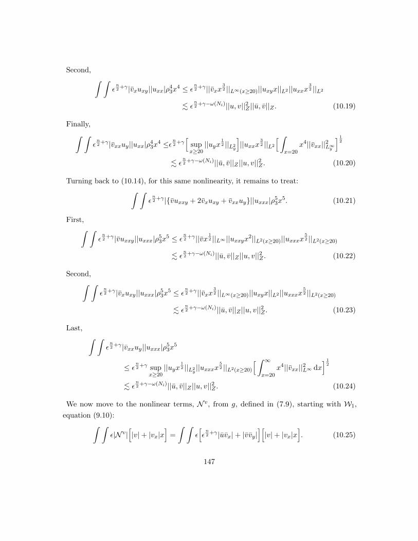
Second, ∫ ∫εn2

+γ |vxuxy||uxx|ρ43x

4 ≤ εn2

+γ ||vxx32 ||L∞(x≥20)||uxyx||L2 ||uxxx

32 ||L2

. εn2

+γ−ω(Ni)||u, v||2Z ||u, v||Z . (10.19)

Finally,∫ ∫εn2

+γ |vxxuy||uxx|ρ43x

4 ≤εn2

+γ[

supx≥20||uyx

12 ||L2

y

]||uxxx

32 ||L2

[ ∫x=20

x4||vxx||2L∞y] 1

2

. εn2

+γ−ω(Ni)||u, v||Z ||u, v||2Z . (10.20)

Turning back to (10.14), for this same nonlinearity, it remains to treat:∫ ∫εn2

+γ |vuxxy + 2vxuxy + vxxuy||uxxx|ρ53x

5. (10.21)

First,∫ ∫εn2

+γ |vuxxy||uxxx|ρ53x

5 ≤ εn2

+γ ||vx12 ||L∞ ||uxxyx2||L2(x≥20)||uxxxx

52 ||L2(x≥20)

. εn2

+γ−ω(Ni)||u, v||Z ||u, v||2Z . (10.22)

Second,∫ ∫εn2

+γ |vxuxy||uxxx|ρ53x

5 ≤ εn2

+γ ||vxx32 ||L∞(x≥20)||uxyx||L2 ||uxxxx

52 ||L2(x≥20)

. εn2

+γ−ω(Ni)||u, v||Z ||u, v||2Z . (10.23)

Last, ∫ ∫εn2

+γ |vxxuy||uxxx|ρ53x

5

≤ εn2

+γ supx≥20||uyx

12 ||L2

y||uxxxx

52 ||L2(x≥20)

[ ∫ ∞x=20

x4||vxx||2L∞ dx] 1

2

. εn2

+γ−ω(Ni)||u, v||Z ||u, v||2Z . (10.24)

We now move to the nonlinear terms, N v, from g, defined in (7.9), starting with W1,

equation (9.10):∫ ∫ε|N v|

[|v|+ |vx|x

]=

∫ ∫ε[εn2

+γ |uvx|+ |vvy|][|v|+ |vx|x

]. (10.25)

147

First, ∫ ∫εn2

+γ+1|uvx| · |v| . εn2

+γ+1||ux14 ||L∞ ||vxx

12 ||L2 ||x−

34 v||L2

. εn2

+γ ||ux14 ||L∞ ||

√εvxx

12 ||L2 ||

√εvxx

14 ||L2 ,

. εn2

+γ−ω(Ni)||u, v||2Z ||u, v||Z , (10.26)∫ ∫εn2

+γ+1|vvy| · |v| . εn2

+γ+1||vx12 ||L∞ ||vyx

12 ||L2 ||vx||L2

. εn2

+γ−ω(Ni)||u, v||2Z ||u, v||Z . (10.27)

Next, ∫ ∫εn2

+γ+1|uvx||vx|x ≤ εn2

+γ+1||u||L∞ ||vxx12 ||L2 ||vxx

12 ||L2 ,

. εn2

+γ−ω(Ni)||u, v||2Z ||u, v||Z , (10.28)∫ ∫εn2

+γ+1|vvy||vx|x ≤ εn2

+γ+1||vx12 ||L∞ ||vyx

12 ||L2 ||vxx

12 ||L2 ,

. εn2

+γ−ω(Ni)||u, v||Z ||u, v||2Z . (10.29)

We will now move to the nonlinear terms, N v, arising from W2, (see equation (9.82)),

which are summarized here:∫ ∫ε|∂xN v|

[|vx|ρ2

2x2 + |vxx|ρ3

2x3]

=

∫ ∫εn2

+γ+1|∂x[uvx + vvy

]|[|vx|ρ2

2x2 + |vxx|ρ3

2x3]

(10.30)

We will go through (10.30) term by term, starting with:∫ ∫εn2

+γ+1|∂x(uvx

)||vx|ρ2

2x2 =

∫ ∫εn2

+γ+1|uxvx + uvxx| · |vx|ρ22x

2

≤ εn2

+γ+1||uxx54 ||L∞(x≥20)||vxx

12 ||L2 ||vxx

12 ||L2

+ εn2

+γ+1||u||L∞ ||vxxx32 ||L2 ||vxx

12 ||L2 ,

≤ εn2

+γ−ω(Ni)||u, v||2Z ||u, v||Z . (10.31)

Staying with this nonlinearity,∫ ∫εn2

+γ+1|uxvx + uvxx| · |vxx|ρ32x

3

≤ εn2

+γ+1||uxx54 ||L∞(x≥20)||vxx

12 ||L2 ||vxxx

32 ||L2

148

+ εn2

+γ+1||u||L∞ ||vxxx32 ||L2 ||vxxx

32 ||L2

. εn2

+γ−ω(Ni)||u, v||2Z ||u, v||Z . (10.32)

We now move to the vvy nonlinearity, still in term (10.30), which we expand:∫ ∫εn2

+γ+1|∂x(vvy

)||vx|ρ2

2x2 =

∫ ∫εn2

+γ+1|vxvy + vvxy||vx|ρ22x

2

≤ εn2

+γ+1||vxx32 ||L∞(x≥20)||vyx

12 ||vxx

12 ||L2

+ εn2

+γ+1||vx12 ||L∞ ||vxx

12 ||L2 ||vxyx

32 ||L2

. εn2

+γ−ω(Ni)||u, v||2Z ||u, v||Z . (10.33)

For this same nonlinear term:∫ ∫εn2

+γ+1|vxvy + vvxy| · |vxx|ρ32x

3

≤ εn2

+γ+1||vxx32 ||L∞(x≥20)||vyx

12 ||L2 ||vxxx

32 ||L2

+ εn2

+γ+1||vx12 ||L∞ ||vxyx

32 ||L2 ||vxxx

32 ||L2

. εn2

+γ−ω(Ni)||u, v||Z ||u, v||2Z . (10.34)

We now move to the highest-order terms, which we read from (9.219), and summarize

here: ∫ ∫εn2

+γ+1|∂xxN v|[|vxx|ρ4

3x4 + |vxxx|ρ5

3x5]

=

∫ ∫εn2

+γ+1|∂xx[uvx + vvy

]|[|vxx|ρ4

3x4 + |vxxx|ρ5

3x5]. (10.35)

We shall expand:∫ ∫εn2

+γ+1|∂xx(uvx

)| · |vxx|ρ4

3x4

=

∫ ∫εn2

+γ+1|uvxxx + 2uxvxx + uxxvx| · |vxx|ρ43x

4. (10.36)

First, ∫ ∫εn2

+γ+1|uvxxx| · |vxx|ρ43x

4 ≤ εn2

+γ+1||u||L∞ ||vxxxx52 ||L2(x≥20)||vxxx

32 ||L2

. εn2

+γ−ω(Ni)||u, v||2Z ||u, v||Z . (10.37)

149

Next,∫ ∫εn2

+γ+1|uxvxx| · |vxx|ρ43x

4 ≤ εn2

+γ+1||uxx54 ||L∞(x≥20)||vxxx

32 ||L2 ||vxxx

32 ||L2

≤ εn2

+γ−ω(Ni)||u, v||2Z ||u, v||Z . (10.38)

Third,∫ ∫εn2

+γ+1|vxuxx||vxx|ρ43x

4 ≤ εn2

+γ+1||vxx32 ||L∞(x≥20)||uxxx

32 ||L2 ||vxxx

32 ||L2

. εn2

+γ−ω(Ni)||u, v||2Z ||u, v||Z . (10.39)

Turning back to (10.35), for this same nonlinearity, we will now treat:∫ ∫εn2

+γ+1|uvxxx + 2uxvxx + uxxvx||vxxx|ρ53x

5 (10.40)

First,∫ ∫εn2

+γ+1|uvxxx||vxxx|ρ53x

5 ≤ εn2

+γ+1||u||L∞ ||vxxxx52 ||L2(x≥20)||vxxxx

52 ||L2(x≥20)

. εn2

+γ−ω(Ni)||u, v||2Z ||u, v||Z . (10.41)

Second,∫ ∫εn2

+γ+1|uxvxx||vxxx|ρ53x

5 ≤ εn2

+γ+1||uxx54 ||L∞(x≥20)||vxxx

32 ||L2 ||vxxxx

52 ||L2(x≥20)

. εn2

+γ−ω(Ni)||u, v||2Z ||u, v||Z . (10.42)

Third,∫ ∫εn2

+γ+1|uxxvx||vxxx|ρ53x

5 ≤ εn2

+γ+1||vxx32 ||L∞(x≥20)||uxxx

32 ||L2 ||vxxxx

52 ||L2(x≥20)

. εn2

+γ−ω(Ni)||u, v||2Z ||u, v||Z . (10.43)

Turning to (10.35), we now approach the final nonlinear term in g (see definition (7.9)),

which is the vvy term. First, we will expand:∫ ∫εn2

+γ+1|∂xx(vvy

)| · |vxx|ρ4

3x4

=

∫ ∫εn2

+γ+1|vxxvy + vxvxy + vvxxy| · |vxx|ρ43x

4. (10.44)

150

First,∫ ∫εn2

+γ+1|vxxvy| · |vxx|ρ43x

4 ≤ εn2

+γ+1||uxx54 ||L∞(x≥20)||vxxx

32 ||L2 ||vxxx

32 ||L2

. εn2

+γ−ω(Ni)||u, v||2Z ||u, v||Z . (10.45)

Second,∫ ∫εn2

+γ+1|vxvxy||vxx|ρ43x

4 ≤ εn2

+γ+1||vxx32 ||L∞(x≥20)||vxyx

32 ||L2 ||vxxx

32 ||L2

. εn2

+γ−ω(Ni)||u, v||2Z ||u, v||Z . (10.46)

Third,∫ ∫εn2

+γ+1|vvxxy||vxx|ρ43x

4 ≤ εn2

+γ+1||vx12 ||L∞ ||vxxyx

52 ||L2(x≥20)||vxxx

32 ||L2

. εn2

+γ−ω(Ni)||u, v||2Z ||u, v||Z . (10.47)

Again turning to (10.35), for this same nonlinearity, we must also treat:∫ ∫εn2

+γ+1|vxxvy + vxvxy + vvxxy| · |vxxx|ρ53x

5. (10.48)

First, ∫ ∫εn2

+γ+1|vxxvy||vxxx|ρ53x

5

≤ εn2

+γ+1||uxx54 ||L∞(x≥20)||vxxx

32 ||L2 ||vxxxx

52 ||L2(x≥20)

≤ εn2

+γ−ω(Ni)||u, v||2Z ||u, v||Z . (10.49)

Second, ∫ ∫εn2

+γ+1|vxvxy||vxxx|ρ53x

5

≤ εn2

+γ+1||vxx32 ||L∞(x≥20)||vxyx

32 ||L2 ||vxxxx

52 ||L2(x≥20)

. εn2

+γ−ω(Ni)||u, v||2Z ||u, v||Z . (10.50)

Finally, ∫ ∫εn2

+γ+1|vvxxy||vxxx|ρ53x

5

≤ εn2

+γ+1||vx12 ||L∞ ||vxxyx

52 ||L2(x≥20)||vxxxx

52 ||L2(x≥20)

151

. εn2

+γ−ω(Ni)||u, v||2Z ||u, v||Z . (10.51)

This now concludes all of the nonlinear terms in Wi. The final task is to control the

Ru,n, Rv,n terms in f, g. Via Lemma 6.27, for κ arbitrarily small and σn as in (6.1), we

choose now σ′ = 110,000 . Then, we have:∣∣∣ ∫ ∫ ε−

n2−γRu,nu+

∫ ∫ε−

n2−γRu,nvyx

∣∣∣ . ε−n2−γ ||Ru,nx

12

+σ′ ||L2 ||x−12−σ′u, x

12 vy||L2

≤ C(n)ε−n2−γ ||||Ru,n||L2

yx

12

+σ′ ||L2x||u, v||X1 (10.52)

≤ C(n)ε14−γ−κ||x−

34

+2σn+σ′+κ||L2x||u, v||X1 (10.53)

≤ C(n)ε14−γ−κ||u, v||X1 . (10.54)

In (10.52), we have used the Hardy inequality with power x−12−σ, which is admissible as

u(1, y) = 0. Upon citing (6.1), one has:

||x−34

+2σn+σ′+κ||L2x|| = ||x−

34

+ 210,000

+ 110,000

+κ||L2x<∞. (10.55)

Next, again via Lemma 6.27, we have:∫ ∫ε1−

n2−γ |Rv,n|

(|v|+ |vx|x

)≤ ε−

n2−γ ||√εRv,nx

12

+σ′ ||L2 ||x−12−σ′√εv, x

12√εvx||L2

. ε14−γ−κ||u, v||X1 . (10.56)

Summarizing these forcing terms:

ε−n2−γ∣∣∣ ∫ ∫ Ru,nu+ εRv,nv +Ru,nvyx+ εRv,nvxx

∣∣∣≤ ε

14−γ−κ + ε

14−γ−κ||u, v||2X1

. (10.57)

Similarly, for higher order terms,∫ ∫ε−

n2−γ |Ru,nx ||ux|ρ2

2x2 + |uxx|ρ3

2x3

. ε14−γ−κ||x−1− 5

4+σ′+κ0x

32 ||L2

x||uxx

12 , uxxρ

322 x

32 ||L2

. ε14−γ−κ||u, v||X1∩X2 . (10.58)

and ∫ ∫ε−

n2−γ |Ru,nxx ||uxx|ρ4

3x4 + |uxxx|ρ5

3x5

152

. ε14−γ−κ||x−2− 5

4+σ′+κx

52 ||L2

x||uxxρ

323 x

32 , uxxxρ

523 x

52 ||L2

. ε14−γ−κ||u, v||X1∩X2∩X3 . (10.59)

For the terms from g:

ε−n2−γ∫ ∫

ε|Rv,nx ||vx|ρ22x

2 + |vxx|ρ32x

3

.ε14−γ−κ||x−1− 5

4+σ′+κx

32 ||L2

x||√εvxx

12 ,√εvxxρ

322 x

32 ||L2

.ε14−γ−κ||u, v||X1∩X2 . (10.60)

and

ε−n2−γ∫ ∫

ε|Rv,nxx ||vxx|ρ43x

4 + |vxxx|ρ53x

5

. ε14−γ−κ||x−2− 5

4+σ′+κx

52 ||L2

x||√εvxxρ

323 x

32 ,√εvxxxρ

523 x

52 ||L2

. ε14−γ−κ||u, v||X1∩X2∩X3 . (10.61)

Combining all of the estimates we have established, we have proven Lemma 10.1.

We may now prove the main result, Theorem 7.1:

Proof of Theorem 7.1. The starting point is estimate (8.118):

||u, v||2Z . ε100 + εn2

+γ−ω(Ni)||u, v||4Z + ||u, v||2X1∩X2∩X3(10.62)

. ε100 + εn2

+γ−ω(Ni)||u, v||4Z +∣∣∣W1 +W2 +W3

∣∣∣ (10.63)

. ε100 + εn2

+γ−ω(Ni)||u, v||4Z + ε14−γ−κ + ε

14−γ−κ||u, v||2X1∩X2∩X3

+ εn2−ω(Ni)||u, v||2Z + ε

n2−ω(Ni)||u, v||4Z , (10.64)

so absorbing the ||u, v|| terms to the left-hand side gives:

||u, v||2Z . ε14−γ−κ + ε

n2−ω(Ni)

(||u, v||4Z

). (10.65)

153

Chapter III: Existence and Uniqueness

11 Overview of Results

With the main estimate, (10.65), in hand, we will prove existence and uniqueness of solutions

to the nonlinear system specified in (7.1) - (7.3), which is defined on the domain Ω, with

boundary conditions given in (7.4), and f, g as in (7.5). The main result of this chapter is:

Theorem 11.1. For ε, δ sufficiently small, ε << δ, κ > 0 small, and 0 ≤ γ < 14 , there exists

a unique solution [u, v] ∈ Z(Ω) to the system (7.1) - (7.3), (7.4), (7.5) satisfying the bound:

||u, v||Z(Ω) . C(uR, vR)ε14−γ−κ. (11.1)

The main result, Theorem 1.2 follows immediately from Theorem 11.1. The proof of this

theorem proceeds in several steps, which we now outline:

(Step 1) Linear existence of solutions to weighted Stokes system, defined as follows:

∆2εψ + αA(ψ) = Fy − εGx on ΩN , F,G ∈ L2(ΩN ), (11.2)

ψ|y=0,N = ψy|y=0,N = 0, and ψ|x=1 = ψx|x=1 = 0, (11.3)

limx→∞

[ψx, ψy] = 0. (11.4)

where α > 0, and

A(ψ) =[ψx2m − ψyyx2m+2 − ∂x(ψxx

2m+2) + ψyyyyx2m+4

+ ∂x

(ψyyxx

2m+4)

+ ∂xx

(ψxxx

2m+4)]. (11.5)

Here, m > 0 is sufficiently large, and can remain temporarily unspecified. The scaled

Bilaplacian is defined as ∆2ε := ∂4

y + ε∂2y∂

2x + ε2∂4

x. The right-hand sides, F,G, should

be thought of as generic elements satisfying Fy − εGx ∈ H−1. Upon introducing

appropriate function spaces, we define the weak formulation of (11.2) - (11.3) in (12.6).

Depicting the weak-solution operator to the above system by S−1α (see 12.12 for a

precise definition), Step 1 amounts to studying the solvability of Sαψ = Fy − εGx.

The boundary conditions as x→∞ in (11.4) are selected in order to be consistent

with (7.4). However, due to the terms in A(ψ), the weak solution, [ψ, u, v] exhibits

rapid decay as x→∞.

154

(Step 2) Linear existence of compact perturbations to Sα. Define the maps:

T [ψ] := ∂y

[− uRψxy − uRxψy − (vR + ε

n2

+γ v)ψyy + uRyψx

]− ε∂x

[uRψxx − vRyψy + vRψxy + vRyψx

], (11.6)

T0[ψ] := T [ψ] + εn2

+γ∂y[vψyy], (11.7)

Ta[ψ] :=[− uRψxy − uRxψy − vRψyy + uRyψx

], (11.8)

Tb[ψ] :=[uRψxx − vRyψy + vRψxy + vRyψx

]. (11.9)

T has a dependence on v, so to be precise we will sometimes write T [ψ; v]. When

there is no danger of confusion, we simply write T [ψ]. The map T0[ψ] is defined to

match the profile terms, Su(u, v), Sv(u, v) (see the definition in (7.6)), when they are

written in terms of the stream function, ψ. We have defined the notation Ta, Tb so

that we can write T0 = ∂yTa − ε∂xTb. In this step, we are interested in establishing

solvability of the system:

Sαψ + T [ψ] = Fy − εGx on ΩN , (11.10)

[ψ = ψx]|x=1 = [ψ = ψy]|y=0 = [ψ = ψy]|y=N = limx→∞

[ψx, ψy] = 0. (11.11)

The essence of the arguments in this step is that upon applying S−1α to both sides

above, S−1α T is seen as a compact perturbation of the identity. Despite ΩN being

unbounded in the x-direction, the required compactness arises from the weights, w,

present in A(ψ) above in (11.5). The solution of (11.10) is known to decay rapidly as

x→∞, due to the presence of A(ψ). This is captured in estimate (13.67).

(Step 3) Nonlinear existence of auxiliary system: we first invite the reader to refer back to

(7.5) and (7.8) - (7.9) for the definitions of f and g. Given this and the definition of

T in (11.6), we define:

f(u, v) := ε−n2−γRu,n + ε

n2

+γ uux, so that f(u, u, v) = f(u, v) + εn2

+γ vuy. (11.12)

The aim of this step is to obtain existence of solutions (which we now index by α and

N for clarity) to the nonlinear system:

Sαψα,N + T [ψα,N ; vα,N ] = fy(u

α,N , vα,N ) + εgx(uα,N , vα,N ) on ΩN . (11.13)

This existence is obtained in the unit ball of Z(ΩN ) via Schaefer’s fixed point theorem.

155

(Step 4) Nonlinear existence of solutions to the system (7.1) - (7.3), with f, g as in (7.5):

By re-applying the analyses in Sections 8 - 9 and in Lemma 10.1, one obtains the

uniform-in-(α,N) estimate: ||uα,N , vα,N ||Z(ΩN ) . O(δ)ε14−γ−κ, which then enables

the passage to weak limits in the space X1 ∩X2 ∩X3. The weak limit is denoted by

[u, v], and is demonstrated to satisfy a weak formulation of system (7.1) - (7.3), see

(15.10) for this formulation. Moreover, [u, v] ∈ X1 ∩X2 ∩X3, gives enough regularity

to upgrade immediately to a strong solution of (7.1) - (7.3).

Remark 11.2. To establish existence, we rely on compactness methods as opposed

to applying a contraction mapping. The essential reason for this is seen by examining

calculation (10.5), in which the structure is not preserved under taking differences.

Remark 11.3. It is important to establish nonlinear existence of the auxiliary

system before establishing nonlinear existence of the system (7.1) - (7.3), as opposed

to jumping from linear existence of (7.1) - (7.3) to nonlinear existence because the

compactness methods we rely on require the weights from αA(ψ).

(Step 5) Nonlinear uniqueness for solutions to the system (7.1) - (7.3), with f, g as in (7.5): In

order to prove uniqueness, we re-apply the estimates in Sections 8 - 9 with weights that

are weaker by x−b, where b < 1, but is arbitrarily close to 1. This step is necessary

(with the weaker weight) due again to the calculation in (10.5), whose structure is

destroyed upon considering differences.

12 Step 1: Invertibility of Weighted Stokes Operator, Sα

In this step, we study the system (11.2) - (11.3). We remind the reader that still, all

integrations and all norms are taken over ΩN unless otherwise specified. There is an abuse

of notation here; ψ should be indexed by α and N , but this will not cause any confusion for

this step, as we view both α and N as fixed. Our intention of this subsection is to exhibit

solvability of the system (11.2) in the space Z(ΩN ). Denote by χ1(x) a cut-off function

satisfying (refer to (8.1) for the definition of ζ3):

χ1 = 1 on x ≥ 12

10, χ1 = 0 for 1 ≤ x ≤ 11

10. (12.1)

We define higher-order cut-offs similar to (12.1), satisfying the following property: support χk ⊂χk−1 = 1. Define the following auxiliary norms via:

||ψ||2H2w

:=

∫ ∫ψ2x2m + |∇ψ|2x2m+2 + |∇2ψ|2x2m+4 (12.2)

156

||ψ||2H3w

:= ||ψ||H2w

+

∫ ∫ ∣∣∣∇2ψx

∣∣∣2x2m+4, (12.3)

||ψ||2Gkw,B

:= ||ψ||2Hkw

+

∫ ∫B

∣∣∣∂kyψ∣∣∣2, for any bounded subset B ⊂ ΩN ,k = 0, ...3, (12.4)

||ψ||2Hkw

:= ||ψ||2H3w

+

∫ ∫χ2k

∣∣∣∇2∂k−2x ψ

∣∣∣2x2m+4, for k ≥ 4. (12.5)

We will also call Gkw,loc(ΩN ) the space such that ||ψ||Gkw,B ≤ C(B) for all compact subsets

B. Define the weak formulation of (11.2) to be:∫ ∫∇2εψ : ∇2

εφ+ α[ ∫ ∫

ψφx2m +

∫ ∫∇ψ · ∇φx2m+2 +

∫ ∫∇2ψ : ∇2φx2m+4

]= 〈Fy − εGx, φ〉H−1,H1 for all φ ∈ C∞0 (ΩN ), where ψ ∈ H2

w(ΩN ). (12.6)

Above, ∇2 is the Hessian matrix, and the inner product between two matrices is given by

A : B = trace(AB). We will need one more norm:

||(F,G)||H−1k

:=

k∑j=0

||∂jxFy − εGx||H−1 . (12.7)

Relevant spaces are defined here:

Definition 12.1. H2w(ΩN ) is defined to be the closure of C∞0 (ΩN ) under the norm || · ||H2

w.

Hkw(ΩN ) for k ≥ 3 consists of the subspace of H2

w(ΩN ) whose Hkw(ΩN ) norm is finite. Note

that H3w(ΩN ) does not contain all of the third derivatives of ψ; it is missing ∂3

yψ, which is

the reason for the norm, || · ||Gw,B .

Remark 12.2. There is a distinction between H2w(ΩN ), and Hk

w(ΩN ) in that:

H2w(ΩN ) = C∞0 (ΩN )

||·||H2w but for k ≥ 3, H3

w(ΩN )ZZ=C∞0 (ΩN )

||·||H3w . (12.8)

Due to the weights, there is no “H = W” theorem generically for Hkw(ΩN ).

Lemma 12.3. For ψ ∈ H2w(ΩN ), the following boundary conditions are satisfied:

ψ|y=0,N = ψy|y=0,N = ψ|x=1 = ψx|x=1 = 0 (12.9)

Proof. If ψ ∈ H2w(ΩN ), obtain a sequence φ(n) such that ||φ(n)−ψ||H2

w→ 0. The claim now

follows by the standard boundedness properties of the trace operator.

Lemma 12.4. H2w(ΩN ) as defined in Definition 12.1 is a Banach space.

157

Proof. Consider the auxiliary space:

H20,w(ΩN ) =

ψ : ∇ψ,∇2ψ exist in the weak sense, and ||ψ||H2

w(ΩN ) <∞. (12.10)

Through standard arguments, H20,w(ΩN ) is a Banach space. Suppose ψ(n) is a Cauchy

sequence in H2w(ΩN ). Then ψ(n) is Cauchy in H2

0,w(ΩN ), and so there exists a limit point

ψ such that: ||ψ−ψ(n)||H2w

n→∞−−−→ 0. As ψ(n) ∈ H2w(ΩN ), we may find a sequence φ(n)

m m≥1

such that ||φ(n)m − ψ(n)||H2

w

m→∞−−−−→ 0, where φ(n)m ∈ C∞0 (ΩN ). In particular, define, for each

n, by selecting m large enough: ||φ(n) − ψ(n)||H2w< 2−n. Thus, ||φ(n) − ψ||H2

w

n→∞−−−→ 0,

proving that ψ ∈ C∞0||·||

H2w . This establishes the desired result.

Lemma 12.5. Endowed with the inner product,

〈ψ,ϕ〉H2w

:=

∫ ∫ψϕx2m +∇ψ · ∇ϕx2m+2 +∇2ψ : ∇2ϕx2m+4, (12.11)

H2w is a Hilbert Space. The inner product in (12.11) induces the norm defined in (12.2).

Proof. One easily verifies the standard axioms of an inner-product for (12.11). Non-

degeneracy of (12.11) is obtained via the boundary conditions in (11.3). Completeness is

then obtained via Lemma 12.4

Definition 12.6. The α−Stokes operator is defined through:

Sαψ = Fy − εGx for ψ ∈ H2w(ΩN ), Fy − εGx ∈ H−1(ΩN ), if and only if (12.6) holds.

(12.12)

It is our aim to study the invertibility of Sα:

Lemma 12.7. Given Fy−εGx ∈ H−1(ΩN ), there exists a unique weak solution ψ ∈ H2w(ΩN )

satisfying (12.6). Such a weak solution satisfies the energy inequality:

||ψ||2H2w.

1

α||Fy − εGx||2H−1 =

1

α||Sαψ||2H−1 . (12.13)

Proof. Define:

B[ψ, φ] :=

∫ ∫∇2εψ : ∇2

εφ+ α[ ∫ ∫

ψφx2m

+

∫ ∫∇ψ · ∇φx2m+2 +

∫ ∫∇2ψ : ∇2φx2m+4

]. (12.14)

158

It is immediate to see that B is bilinear, bounded, and coercive on H2w(ΩN ). Next, Fy−εGx

act as bounded linear functionals on H2w(ΩN ) through the pairing: 〈Fy − εGx, φ〉H−2

w ,H2w

:=

〈Fy − εGx, φ〉H−1,H1 . This follows from:∣∣∣〈Fy − εGx, φ〉H−1,H1

∣∣∣ ≤ ||Fy − εGx||H−1 ||φ||H2w.

The existence of ψ ∈ H2w(ΩN ) a solution to (12.6) is then a standard application of the

Lax-Milgram Lemma to the Hilbert Space H2w(ΩN ). The energy identity above follows from

density of C∞0 (ΩN ) in H2w(ΩN ), which enables us to replace φ with ψ in (12.6).

The above lemma then says that S−1α : H−1(ΩN )→ H2

w(ΩN ) is well-defined. Our intention

now is to upgrade regularity.

Lemma 12.8. Given Fy− εGx ∈ H−1(Ω), the unique weak solution in H2w(ΩN ) guaranteed

by Lemma 12.7 is in H3w(ΩN ) and satisfies:

||ψ||2H3w.

1

α||Fy − εGx||2H−1 =

1

α||Sαψ||2H−1 . (12.15)

Proof. As our weak solutions are only in H2w(ΩN ), we must formally use difference quotients

within the weak formulation (12.6) to upgrade to H3w(ΩN ). However, we will generate the

H3w estimate via differentiating (11.2), with the understanding that everything that is done

can be formalized through the use of difference quotients in the standard manner. As such,

we take ∂x of the system (11.2), which gives:

∆2εψx + αA(ψx) + [∂x, αA]ψ = ∂x(Fy − εGx), (12.16)

where

[∂x, αA]ψ = α[2mx2m−1ψ − (2m+ 2)x2m+1ψyy − (2m+ 2)∂x(ψxx

2m+1)

+ (2m+ 4)x2m+3ψyyyy + (2m+ 4)∂x

(ψyyxx

2m+3)

+ (2m+ 4)∂xx

(ψxxx

2m+3))]. (12.17)

Let χ1 be as above in (12.1). Define the quantities:

χ1 = 1− χ1, ρM (x) = χ1(x)χ1(x

M), which implies

∣∣∣xk∂kxρM (x)∣∣∣ ≤ 2. (12.18)

We now test the above equation, (12.16), against the multiplier ρMψx. Doing so first gives

from the Bilaplacian:∫ ∫∆2εψx · ρMψx =

∫ ∫ρM

[ε|ψxxy|2 + ε2|ψxxx|2 + |ψxyy|2

]159

+ c0

∫ ∫ρ′′M

[ε|ψxy|2 + ε2|ψxx|2

]+ c1

∫ ∫∂4xρM · |ψx|2, (12.19)

for constants c0, c1. Next, we have the terms coming from A:∫ ∫αA(ψx) · ρMψx

& α

∫ ∫[ψ2xx

2m + ψ2xyx

2m+2 + ψ2xxx

2m+4 + ψ2xyyx

2m+4

+ ψ2xxyx

2m+4 + ψ2xxxx

2m+4]ρM − ||ψ||2H2w. (12.20)

Through a direct integration by parts, the commutator contains lower order terms:∣∣∣ ∫ ∫ [∂x, αA]ψ · ψxρM∣∣∣ . ||ψ||2H2

w.

1

α||Fy − εGx||2H−1 . (12.21)

For detailed proofs of calculations (12.20) and (12.21), we refer the reader to (13.99) -

(13.106). Finally, on the right-hand side of (12.16), we have:∣∣∣〈∂x(Fy − εGx), ψxρM 〉H−2,H2

∣∣∣ ≤ ||Fy − εGx||H−1 ||ρMψxx||H1 . (12.22)

We can send M →∞ so that the weight ρM ↑ χ1, resulting in∫ ∫χ1

∣∣∣∇2ψx

∣∣∣2x2m+4 .1

α||Fy − εGx||2H−1 . (12.23)

For the region 1 ≤ x ≤ 20, and 0 ≤ y ≤ N , we apply the standard H2(ΩN ) estimate for

solutions, uα, vα Stokes’ equation near corners (see [BR80], Theorems 1 and 2, and Figure

2, P. 562 also in [BR80] with “C/C” boundary conditions). Formally, fix another cut-off

function, χ2(x, y) localized near the corner (1, 0) (the identical argument can be given for

the other corner, (1, N)). First, by calculation, we have:

∆2ε

(χ2ψ

)= χ2∆2

εψ + [∆2ε , χ]ψ, (12.24)

where the expression for the commutator is given explicitly:

[∆ε, χ2]ψ = 4∂yχ2∂3yψ + 4∂3

yχ2∂yψ + 6∂2yχ2∂

2yψ + 2ε∂2

x∂2yχ2ψ + 2ε∂2χ2∂

2xψ

+ 4ε∂x∂2yχ2∂xψ + 2ε∂2

xχ2∂2yψ + 4ε∂xχ2∂x∂

2yψ + 4ε∂2

x∂yχ2∂yψ

+ 4ε∂yχ2∂2x∂yψ + 8ε∂xyχ2∂xyψ + 6ε2∂2

xχ2∂2xψ + ε2∂4

xχ2ψ + 4ε2∂3xχ2∂xψ

+ 4ε2∂xχ2∂3xψ. (12.25)

160

The salient feature of (12.25) will be:

[∆ε, χ2]ψ = o(χ2∂3ψ), (12.26)

where this is short-hand notation for containing up to three ψ-derivatives, and localized

by χ2 (or any derivative of χ2 which is also localized). Localizing (11.2) using χ2:

||χ2ψ||H3 . ||χ2(Fy − εGx)||H−1 + ||o(χ2∂3ψ)||H−1 . ||χ2(Fy − εGx)||H−1 . (12.27)

Combining (12.27) and (12.23) gives the desired result.

Lemma 12.9. Fix any bounded set B ⊂ ΩN . Then we have:

||ψ||2G3w,B

. C(B)1

α||Fy − εGx||2H−1 , (12.28)

where the constant C(B) depends on B.

Proof. This argument proceeds identically to the calculation from the previous lemma

which resulted in (12.27) by simply replacing χ2 with cut-off functions localized to each

interval x ∈ [M,M + 1]. The dependence on B in the constant in (12.28) arises from the

weights x2m, x2m+2, x2m+4 appearing in the equation (11.2) through A(ψ).

The above lemmas roughly show that S−1α gains four derivatives. By repeating this

procedure for higher-order x-derivatives, we can upgrade to higher-regularity:

Lemma 12.10. Given (F,G) ∈ H−12 , the unique weak solution guaranteed by Lemma 12.7

satisfies:

||ψ|2H5w.

1

α||(F,G)||2

H−12

(12.29)

For (F,G) ∈ H−12 , we can upgrade weak solutions to strong solutions:

Lemma 12.11. Given (F,G) ∈ H−12 , the unique weak solution guaranteed by Lemma 12.7

is a strong solution of (11.2).

Proof. An integration by parts of the weak formulation (12.6), justified according to the

previous lemma, is equivalent to the equation (11.2) being satisfied pointwise on ΩN . The

boundary conditions at x = 1, y = 0, y = N are satisfied by Lemma 12.3. The boundary

condition at x→∞ comes from the norms, (12.2), which when applying with k = 5, imply

that up to four derivatives of ψ vanish rapidly at x→∞.

161

13 Step 2: Compact Perturbations, Sαψ + T [ψ]

For this step, we invite the reader to refer back to the specification of T [ψ], given in (11.6),

and the system that we will focus on, given in (11.10). Note that T [ψ] contains a loss of

three-derivatives for ψ. Note also the presence of the term εn2

+γ v. We will now need some

compactness lemmas.

Lemma 13.1. Fix two weights, w1 = xm1 , and w2 = xm2 , where m2 > m1 ≥ 0. Then, one

has the following compact embedding:

H1loc(Ω

N ) ∩ L2w2

(ΩN ) →→ L2w1

(ΩN ). (13.1)

Proof. Consider a family of functions fn defined on ΩN such that:

supn

∫ ∫f2nw

22 <∞, (13.2)

and such that fn ∈ H1loc(Ω

N ), uniformly in n. By taking Sobolev extensions across ∂ΩN ,

and subsequently cutting off in the y and negative x directions, we can assume fn are

defined on R2, compactly supported in the y direction and negative x direction. Fix any

δ′ > 0. Since m2 > m1, there exists a compact set K = K(δ′) such that:

supn||fn||L2

w1(Kc) ≤

δ′

2. (13.3)

On K, by Rellich compactness, there exists a subsequence (depending on δ′) such that

lim supj,k→∞

||fnj − fnk ||L2(K) ≤δ′

2× diam(K)m1. (13.4)

Then,

lim supj,k→∞

||fnj − fnk ||L2w1

(K) ≤δ′

2. (13.5)

Combining the above two estimates,

lim supj,k→∞

||fnj − fnk ||L2w1≤ δ′. (13.6)

Taking successively δ′ = 2−n and applying a diagonalization argument gives the result.

162

Lemma 13.2. Let the weight, x2m, in the expression for A(ψ), equation (11.5), be selected

for any m > 0. Then the map S−1α T is well-defined and compact H2(ΩN )→ H2(ΩN ).

Proof. According to (12.28), this follows from the compactness of G3w,loc(Ω

N ) →→ H2(ΩN ),

which in turn follows from (13.1). The lemma is proven.

We are now ready to study system (11.10). The first task is to obtain an energy estimate

to the inhomogeneous problem:

Lemma 13.3. Suppose ψ ∈ H2(ΩN ) is a solution to (11.10), where (F,G) ∈ H−12 , and

||u, v||Z ≤ 1. Then ψ obeys the following energy estimate:

||uy||2L2 + α||ψ||2H2w. O(δ)||

√εvxx

12 , vyx

12 ||2L2 +

∫ ∫Fu+ ε|G||v|. (13.7)

Proof. Supposing there existed such a ψ, we would have T [ψ] ∈ H−1(ΩN ), and so by (12.15),

we know ψ ∈ H3w(ΩN ). By bootstrapping this regularity, we obtain that:

ψ ∈ H5w(ΩN ). (13.8)

We would like to apply the multiplier ψ to the equation (11.10) in order to repeat the

energy estimate from Proposition 9.2. Select test functions, φ(n) ∈ C∞0 (ΩN ), which satisfy:

||φ(n) − ψ||H2w→ 0. (13.9)

This is possible according to the density of C∞0 (ΩN ) in H2w in Definition 12.1. Multiplying

(11.10) by φ(n), then gives on the left-hand side:∫ ∫ (∆2εψ + Tψ

)· φ(n) + α

∫ ∫A(ψ)φ(n). (13.10)

First, we shall use (11.7) to write:∫ ∫ (∆2εψ + T [ψ]

)φ(n) =

∫ ∫ (∆2εψ + T0[ψ]

)φ(n) −

∫ ∫εn2

+γ∂y(vuy) · φ(n)

=

∫ ∫ (∆2εψ + T0[ψ]

)φ(n) +

∫ ∫εn2

+γ(vuy) · φ(n)y . (13.11)

According to (13.9), we pass to limits in the following terms:∫ ∫(∆2

εψ + T0[ψ])φ(n) =

∫ ∫∇2εψ : ∇2

εφ(n) +

∫ ∫T0[ψ]φ(n)

163

n→∞−−−→∫ ∫

|∇2εψ|2 +

∫ ∫T0[ψ]ψ. (13.12)

We have used:

|∫ ∫

T0[ψ]φ(n) − T0[ψ]ψ| =∫ ∫

(∂yTa[ψ]− ∂xTb[ψ]) · (φ(n) − ψ)

≤ ||Ta[ψ], Tb[ψ]||L2 ||φ(n) − ψ||H1

≤ ||ψ||H5w||φ(n) − ψ||H1

n→∞−−−→ 0, (13.13)

according to (13.8) and the definition in equation (11.7). The integration on the right-hand

side of (13.12) arises exactly from the energy estimates, Proposition 9.2, in particular, terms

(9.12), (9.29), (9.41), and so we may write:

| limn→∞

∫ ∫ (∆2εψ + T0[ψ]

)φ(n)| & ||uy||2L2 −O(δ)||

√εvxx

12 , vyx

12 ||2L2 . (13.14)

We may pass to the limit in the final term of (13.11) due to the calculation:

|∫ ∫

vuy(φ(n)y − ψy)| ≤ ||v||L∞ ||uy||L2 ||φ(n)

y − ψy||L2

≤ ε−N4 ||v||Z ||uy||L2 ||φ(n)y − ψy||L2

n→∞−−−→ 0. (13.15)

Upon passing to the limit, we integrate by parts:

−∫ ∫

εn2

+γ(vuy) · φ(n)y

n→∞−−−→∫ ∫

εn2

+γ(vuy) · u = −∫ ∫

εn2

+γ

2vyu

2 (13.16)

From here, we estimate identically as in (10.5):

|∫ ∫

εn2

+γ

2vyu

2| ≤ εn2

+γ−ω(Ni)||u, v||Z ||vyx12 ||2L2 ≤ ε

n2

+γ−ω(Ni)||vyx12 ||2L2 . (13.17)

It remains to treat (13.10), for which we use the compact support of φ(n) to justify the

integration by parts:∫ ∫αA(ψ) · φ(n) =

∫ ∫ψφ(n)x2m +∇ψ · ∇φ(n)x2m+2 +∇2ψ : ∇2φ(n)x2m+4. (13.18)

Passing to the limit, according to (13.9):

limn→∞

∫ ∫αA(ψ)φ(n) = α

∫ ∫ψ2x2m + |∇ψ|2x2m+2 + |∇2ψ|2x2m+4, (13.19)

164

On the right-hand side, we have:∫ ∫Fy · φ(n) = −

∫ ∫Fφ(n)

yn→∞−−−→

∫ ∫Fu, (13.20)∫ ∫

−εGx · φ(n) =

∫ ∫εG · φ(n)

xn→∞−−−→

∫ ∫εGv. (13.21)

Consolidating the previous estimates gives the desired estimate, (13.7).

The task now is to estimate the right-hand side of (13.7) in terms of the left-hand side

using the smallness of O(δ). We refer the reader to Proposition 9.4, whose proof we follow

closely. We will point out the subtle differences:

Lemma 13.4. Suppose ψ ∈ H2(ΩN ) is a solution to (11.10), where (F,G) ∈ H−12 , and

||u, v||Z ≤ 1. Suppose the weight w = x2m from equation (11.5) is selected such that m is

sufficiently large relative to universal constants. Then ψ obeys:

||√εvx, vyx

12 ||2L2 . ||uy||2L2 + α||ψ||2H2

w+

∫ ∫|F ||ux|x+ ε|G||v|+ ε|G||vx|x. (13.22)

Proof. We will repeat the positivity estimate of Proposition 9.4. To do so, we apply the

multiplier ψxxχ2L,α to (11.10). Here, χ is a normalized cut-off function equal to 1 on [1, 2]

and 0 on [3,∞), and

χL,α(x) := χ(α

Lx), so that ∂kxχL,α =

αk

Lkχ(k). (13.23)

Such a cut-off function was not present in Proposition 9.4. The necessity of it is due to

the terms arising from A(ψ). The presence of this cut-off function enables us to justify

all integrations by parts in the x-direction. For our fixed α > 0, we will eventually send

L→∞. Applying the multiplier ψxxχ2L,α to (11.10), gives on the left-hand side:∫ ∫ (

T [ψ] + ∆2εψ)· ψxxχ2

L,α + α

∫ ∫A(ψ) · ψxxχ2

L,α (13.24)

=

∫ ∫ (T0[ψ] + ∆2

εψ + εn2

+γ∂y[vuy])· ψxxχ2

L,α + α

∫ ∫A(ψ) · ψxxχ2

L,α.

We will first focus on the first two integrands above in (13.24), which appeared in

Proposition 9.4. The obstacle to repeating the calculations exactly as in Proposition 9.4

is the presence of the cut-off function, χ2L,α, in the multiplier. The essential idea is this:

165

when no derivative falls on χ2L,α, the estimate will be the same as the corresponding term

in Proposition 9.4. When at least one derivative falls on χ2L,α, we may use the factors of

α obtained from the scaling in (13.23) to absorb the new terms into the left-hand side of

(13.7). Let us start with the profile terms from T0[ψ], for which we refer the reader to

estimates (9.64) - (9.68). We will transfer all of the terms to velocity formulation so as to

remain consistent with estimates (9.64) - (9.68).∫ ∫∂ySu · vxχ2

L,α =

∫ ∫Suuxxχ

2L,α

=

∫ ∫[uRux + uRxu+ vRuy + uRyv]uxxχ

2L,α

&∫ ∫

u2xxχ

2L,α − |

∫ ∫[uRxu+ vRuy + uRyv]uxxχ

2L,α|. (13.25)

We will treat the three terms on the right-hand side above, using (2.12) and (2.18) starting

with: ∫ ∫uRxuxuxχ

2L,α =

∫ ∫uPRx + uERxuxuxχ2

L,α

≤ ||yx12uPRx||L∞ ||uy||L2 ||vyx

12χL,α||L2

+ ||uERxx32 ||L∞ ||

u

xχL,α||L2 ||uxx

12χL,α||L2

≤ O(δ)||uy||2L2 +O(δ)||uxx12χL,α||2L2 +

α

L||u||2L2

≤ O(δ)||uy||2L2 +O(δ)||uxx12χL,α||2L2 +

α

L||ψ||2H2

w. (13.26)

Above, we have used the Hardy inequality:

||uxχL,α||L2 . ||∂x(uχL,α)||L2 ≤ ||uxχL,α||L2 +

α

L||uχ′L,α||L2

. ||uxχL,α||L2 +α

L||ψ||H2

w. (13.27)

Next, by (2.10), (2.20), we have:∣∣∣ ∫ ∫ vRuyvyxχ2L,α

∣∣∣ ≤ ||vRx 12 ||L∞ ||uy||L2 ||vyx

12χL,α||L2

≤ O(δ)||uy||L2 ||vyx12χL,α||L2 . (13.28)

Next, by (2.14), (2.16), (2.18) we have:∫ ∫uRyvuxxχ

2L,α =

∫ ∫uPRy +

√εuERY vvyxχ2

L,α

166

≤ ||yuPRy||L∞ ||vyx12χL,α||2L2

+√ε||uERY x

32 ||L∞ ||vyx

12χL,α||L2 ||

√εv

xχL,α||L2

≤ ||yuPRy||L∞ ||vyx12χL,α||2L2

+√ε||uERY x

32 ||L∞ ||vyx

12χL,α||L2 ||

√εvxχL,α||L2

+α

L

√ε||uERY x

32 ||L∞ ||vyx

12χL,α||L2 ||

√εvχ′L,α||L2

≤ O(δ)||vyx12χL,α||2L2 +

√εO(δ)||

√εvxχL,α||2L2 +O(δ)

α

L||ψ|2H2

w.

(13.29)

Summarizing the previous four terms:∫ ∫∂ySu · vxχ2

L,α & ||vyx12χL,α||2L2 −

α

L||ψ||2H2

w

−O(δ)||uy||2L2 −O(δ)√ε||√εvxχL,α||2L2 . (13.30)

We will now move to the profile terms from Sv, which are located starting from estimate

(9.69). First,∫ ∫−ε∂xSv · vxχ2

L,α =

∫ ∫εSv · [vxxχ2

L,α + vχ2L,α + vx

2α

LχL,αχ

′L,α]. (13.31)

Referring to definition (7.5), consider the term uRvx in Sv, which is the most delicate

profile term: ∫ ∫εuRv

2xxχ

2L,α +

∫ ∫εuRvxv[χL,α + 2x

α

LχL,αχ

′L,α]. (13.32)

The first term above in (13.32) gives positivity:∫ ∫εuRv

2xxχ

2L,α &

∫ ∫εv2xxχ

2L,α. (13.33)

We will treat the second term on the right-hand side of (13.32):∫ ∫εuRvvxχ

2L,α = −

∫ ∫εv2

2[uRxχ

2L,α + 2uR

α

LχL,αχ

′L,α], (13.34)∫ ∫

εuRvvxxα

LχL,αχ

′L,α = −

∫ ∫εv2

2[uRxx

α

LχL,αχ

′L,α

+ uRα

LχL,αχ

′L,α + uRx

α2

L2χL,αχ

′′L,α]. (13.35)

167

The first term on the right-hand side of (13.34) yields:

|∫ ∫

εv2uRxχ2L,α| .

√ε||χL,α

√εvx, vyx

12 ||2L2 +

α

L||ψ||2H2

w, (13.36)

in nearly an identical manner to estimate (9.43). We now estimate:

|∫ ∫

εuR2v2α

Lχ′L,α| .

∫ ∫εv2α

L.α

L||ψ||2H2

w. (13.37)

This same estimate can be performed for all the terms in (13.35). Consolidating these

bounds: ∫ ∫εv2xxχ

2L,α . (13.32) +

√ε||χL,α

√εvx, vyx

12 ||2L2 +

α

L||ψ||H2

w. (13.38)

It remains now to treat the remaining three terms in Sv. The second, third, and fourth

terms from Sv can be controlled in the same manner as in (9.71) - (9.73):

ε|∫ ∫

vRxuvxxχ2L,α| ≤

√ε||x

32 vRx||L∞ ||

√εvxx

12χL,α||L2 ||uxχL,α||L2 +

α

L||ψ||2H2

w. (13.39)

ε∣∣∣ ∫ ∫ vRvyvxxχ

2L,α

∣∣∣ ≤ √ε||vR||L∞ ||vyx 12χL,α||L2 ||

√εvxx

12χL,α||L2 +

α

L||ψ||2H2

w. (13.40)

ε∣∣∣ ∫ ∫ vRyvvxxχ

2L,α

∣∣∣ ≤ √ε||vPRyy||L∞ ||vyx 12χL,α||L2 ||

√εvxx

12χL,α||L2

+√ε||vERY x

32 ||L∞ ||

√εvxx

12χL,α||2L2 +

α

L||ψ||2H2

w. (13.41)

We now turn back to (13.31), addressing the second term in the bracket for the final three

profile terms from Sv: ∫ ∫[vRxu+ vRvy + vRyv] · εvχ2

L,α. (13.42)

First, through the Hardy inequality and (2.8), (2.17):

|∫ ∫

εvRxuvχ2L,α| ≤

√ε||x

32 vRx||L∞ ||

u

x34

χL,α||L2 ||√εv

x34

χL,α||L2

≤√ε[||uxx

14χL,α||2L2 + ||

√εvxx

14χL,α||2L2 +

α

L||u,

√εvx

14χ′L,α||2L2

]≤√ε[||uxx

14χL,α||2L2 + ||

√εvxx

14χL,α||2L2 +

α

L||ψ||2H2

w

], (13.43)

so long as w = xm is selected larger than x14 , which is true by the assumption of this

lemma. Next, through an integration by parts and (2.10), (2.20):∫ ∫[vRvy + vRyv]εvχ2

L,α =1

2

∫ ∫vRyv

2εχ2L,α ≤ ε||vPRyy2||L∞ ||vyχL,α||2L2

168

+√ε||vERY x

32 ||L∞ ||

√εvxx

14χL,α||2L2 +

α

L||ψ||2H2

w. (13.44)

The final task for the Sv profile contributions is the third term from (13.31):

|∫ ∫

ε[vRxu+ vRvy + vRyv] · vx2α

LχL,αχ

′L,α| ≤

α

L||ψ||2H2

w, (13.45)

so long as w = xm is selected larger than x, which is true by assumption of this lemma.

Let us consolidate all of the calculations from Sv:∫ ∫−ε∂xSv · vxχ2

L,α &∫ ∫

εv2xxχ

2L,α −

√ε||χL,α

√εvx, vyx

12 ||2L2 −

α

L||ψ||2H2

w. (13.46)

It now remains to come to those terms contributed by ∆2εψ into (13.24). We will follow

closely the calculations from (9.52) - (9.63) in Proposition 9.4. We will again omit the

justifications near the corners of our domain as these are identical to Proposition 9.4. Again,

we will write these terms in the velocity form, to remain consistent with the calculations in

(9.52) - (9.63). First,

|∫ ∫

−uyyuxxχ2L,α| = | −

∫ ∫u2y

2[χ2L,α + 2x

α

LχL,αχ

′L,α]| . ||uy||2L2 . (13.47)

Next,∫ ∫−εuxxuxxχ2

L,α| = |∫ ∫

εu2x

2[χ2L,α + 2x

α

LχL,αχ

′L,α] . ε||uxχL,α||2L2 + ε

α

L||ψ||2H2

w.

(13.48)

We now move to the terms from ∆εv, starting with:

|∫ ∫

ε2vxxx · vxχ2L,α| = |

∫ ∫ε2vxx · [vxxχ2

L,α + vχ2L,α + 2vx

α

LχL,αχ

′L,α]|

≤ ε||√εvxχL,α||2L2 +

α

L||ψ||2H2

w. (13.49)

Finally, we have:

|∫ ∫

−εvxyyvxχ2L,α| = |

∫ ∫εvxyvyxχ

2L,α|

= |∫ ∫

εv2y [χ

2L,α + 2x

α

LχL,αχL,α]|

. ε||vyχL,α||2L2 +α

L||ψ||2H2

w. (13.50)

169

By combining calculations (13.30), (13.46), (13.47) - (13.50), and absorbing relevant terms

to the left-hand side below, we have:

||√εvx, vyx

12χL,α||2L2 . ||uy||2L2 +

α

L||ψ||2H2

w

+ α

∫ ∫A(ψ) · ψxxχ2

L,α +

∫ ∫εn2

+γ vuyuxxχ2L,α

+

∫ ∫Fy · vxχ2

L,α − εGx · vxχ2L,α. (13.51)

Via direct integration by parts, which is justified due to the presence of the cut-off function

in x, we compute: ∣∣∣α ∫ ∫ A(ψ)ψxxχ2L,α

∣∣∣ . α||ψ||2H2w. (13.52)

Let us compute each term in A(ψ) to verify (13.52), referring to the definition in (11.5),

starting with:

|∫ ∫

αψx2mvxχ2L,α| = | −

α

2

∫ ∫ψ2∂x[x2m+1χ2

L,α]|

= | − α

2

∫ ∫ψ2[Cx2mχ2

L,α + 2x2m+1α

LχL,αχ

′L,α]| (13.53)

≤ α||ψ||2H2w. (13.54)

For the second term in (13.53), we have used: |αLxχL,α| . 1. Next, let us turn to:

α

∫ ∫(−ψyyx2m+2 + ψyyyyx

2m+4)vxχ2L,α

= α

∫ ∫uyvx

2m+3χ2L,α − αuyuxyx2m+5χ2

L,α

= α

∫ ∫uuxx

2m+3χ2L,α + αu2

y∂x(x2m+5χ2L,α)

. α

∫ ∫u2x2m+2 + u2

yx2m+4 . α||ψ||2H2

w. (13.55)

Next,

α

∫ ∫∂x(ψxx

2m+2)vxχ2L,α = α

∫ ∫vx2m+2∂x(vxχ2

L,α)

= α

∫ ∫vx2m+2[vxxχ

2L,α + vχ2

L,α + 2vxα

LχL,αχ

′L,α]

. α

∫ ∫v2x2m+2 . α||ψ||2H2

w. (13.56)

170

Next,

α

∫ ∫∂x(ψyyxx

2m+4)vxχ2L,α = α

∫ ∫∂x(ψxyx

2m+4)vyxχ2L,α

= α

∫ ∫∂x(uxx

2m+4)uxxχ2L,α . α

∫ ∫u2xx

2m+4 . α||ψ||2H2w.

(13.57)

The final term in A(ψ) is:

α

∫ ∫∂xx(ψxxx

2m+4)vxχ2L,α = α

∫ ∫ψxxx

2m+4∂xx[vxχ2L,α]

= α

∫ ∫vxx

2m+4[vxxxχ2L,α + 2vx∂x(xχL,α) + v∂xx(xχL,α)]

. α||ψ||2H2w. (13.58)

This concludes all the terms in A(ψ), according to (11.5). Estimating the next term in

(13.51) exactly as in (10.8) yields:

|∫ ∫

εn2

+γ vuyuxxχ2L,α| ≤ ε

n2

+γ−ω(Ni)||u, v||Z ||uy||L2 ||uxx12χL,α||L2

≤ εn2

+γ−ω(Ni)||uxx12χL,α||2L2 + ε

n2

+γ−ω(Ni)||uy||2L2 . (13.59)

Finally, we come to the right-hand side:∫ ∫[Fy − εGx] · vxχL,α =

∫ ∫FuxxχL,α + εG∂x[vxχL,α]

≤∫ ∫

|F ||ux|x+ |∫ ∫

εG[vxxχL,α + vχL,α + vx(α

L)χ′L,α]|

≤∫ ∫

|F ||ux|x+ ε|G||vx|x+ ε|G||v|., (13.60)

Inserting the previous few calculations into estimate (13.51) gives:

||√εvx, vyx

12χL,α||2L2 . ||uy||2L2 +

α

L||ψ||2H2

w

+ α||ψ||2H2w

+

∫ ∫|F ||ux|x+ ε|G|[|vx|x+ |v|]. (13.61)

We now send L → ∞, and appeal to Monotone Convergence Theorem, as χL,α ↑ 1 to

establish the desired result.

171

Having understood the inhomogeneous problem:

Lemma 13.5. For (F,G) ∈ H−12 , and ||u, v||Z ≤ 1, there exists a unique weak solution

ψ ∈ H2w(ΩN ) to the system (11.10).

Proof. We apply S−1α to both sides of (11.10), which is valid as the right-hand side and

therefore the left-hand side is assumed to be in at least H−1(ΩN ), thereby yielding:

ψ + S−1α Tψ = S−1

α

(Fy − εGx

). (13.62)

We will study the equation (13.62) as an equality in the space H2(ΩN ). According to the

Fredholm alternative, which is available according to Lemma 13.2, there either exists a

unique solution ψ ∈ H2(ΩN ) to the system (13.62), or a non-trivial solution ψ ∈ H2(ΩN )

to:

ψ + S−1α Tψ = 0 ⇐⇒ Sαψ = −Tψ. (13.63)

Therefore, coupling (13.22) with (13.7), taking F = G = 0, we have:

||√εux, uy||2L2 + α||ψ||2H2

w+ ||√εvxx

12 , vyx

12 ||2L2 ≤ 0, (13.64)

implying ψ, u, v = 0. Thus, by the Fredholm alternative, there exists a unique solution

ψ ∈ H2(ΩN ) to (13.62). Rearranging (13.62):

ψ = S−1α

(Fy − εGx − Tψ

), (13.65)

where Fy−εGx−Tψ ∈ H−1(ΩN ), and so an application of (12.13) shows that ψ ∈ H2w(ΩN ).

This concludes the proof.

Lemma 13.6. Let ψ be the unique H2w(ΩN ) weak solution from Lemma 13.5. Then for

(F,G) ∈ H−12 , ψ ∈ H5

w(ΩN ).

Proof. Tψ ∈ H−1(ΩN ), and so Sαψ = −Tψ + Fy − εGx ∈ H−1(ΩN ), which implies that

ψ ∈ H3w(ΩN ) according to (12.15). Iterating this regularity then gives ψ ∈ H5

w(ΩN ).

We now introduce more notation, which is more suitable for the velocities:

Lα,v[u, v] = (f , g) ⇐⇒ Sαψ + T [ψ; v] = fy − εgx. (13.66)

Summarizing the established results, we have:

172

Corollary 13.7. For f , g ∈ H−12 (ΩN ), α > 0, and ||u, v||Z(ΩN ) ≤ 1, the map Lα,v[u, v] is

invertible, where

L−1α,v : (f , g) ∈ H−1

2 (ΩN )→ [u, v] ∈ H4w(ΩN ). (13.67)

Moreover, the boundary conditions (11.3) are satisfied by [u, v] = L−1α,v[f , g].

It is now our intention to repeat the second and third order energy and positivity estimates

from Section 9, with our new system (11.10). For this, we will need to understand several

calculations. First, we introduce some norms:

||ψ||2J2 := ||ψ||2H2w, (13.68)

||ψ||2Jk+2 :=

∫ ∫|∂kxψ|2(ρk+1)2kx2m+2k + |∇∂kxψ|2ρ2k

k+1x2m+2k+2 (13.69)

+ |∇2∂kxψ|2ρ2kk+1x

2m+2k+4 for k ≥ 1. (13.70)

The reader is referred to the definitions of ρk provided in (8.2). The essential difference

between these Jk-norms and the Hkw norms introduced in (12.2) are the growing weights of

x which each application of ∂x, which mimics the structure of the energy norms, Xk, in

(8.3).

Lemma 13.8.∫ ∫A(∂kxψ) · ∂kxψx2kχ2

L,αρ2kk+1 & ||χL,αψ||2Jk+2 −

k−1∑i=0

||ψ||2Ji+2 (13.71)

Proof. Referring to (11.5), the first term is:∫ ∫|∂kxψ|2x2mx2kχ2

L,αρ2kk+1. (13.72)

The next terms, via an integration by parts in y:∫ ∫−∂kxψyyx2m+2 · ∂kxψx2kρ2k

k+1χ2L,α =

∫ ∫|∂kxψy|2x2m+2k+2ρ2k

k+1χ2L,α, (13.73)∫ ∫

∂kxψyyyyx2m+4 · ∂kxψx2kρ2k

k+1χ2L,α =

∫ ∫|∂kxψyy|2x2m+2k+4ρ2k

k+1χ2L,α. (13.74)

Next,∫ ∫∂x[(∂kxψ)yyxx

2m+4] · ∂kxψx2kχ2L,αρ

2kk+1

173

=

∫ ∫∂k+1x ψyx

2m+4 · ∂x[∂kxψyx2kχ2

L,αρ2kk+1] (13.75)

&∫ ∫

|∂k+1x ψy|2x2m+2k+4χ2

L,αρ2kk+1 −

∫ ∫|∂kxψy|2x2m+2k+2ρ

2(k−1)k (13.76)

&∫ ∫

|∂k+1x ψy|2x2m+2k+4χ2

L,αρ2kk+1 −

k−1∑i=0

||ψ||Ji+2 . (13.77)

Above, we have used the calculation:

∂x[x2kχ2L,αρ

2kk+1] = 2kx2k−1χ2

L,αρ2kk+1 + x2k 2α

LχL,αχ

′L,αρ

2kk+1

+ x2kχ2L,α2kρ2k−1

k+1 ρ′k+1. (13.78)

For the second term on the right-hand side of (13.78), we estimate: 2αL xχL,α . 1. For the

third term on the right-hand side, we use that the support of ρ′k+1 is localized in x. We

also use that: support(ρk) ⊂ ρk−1 = 1. Next, we integrate by parts twice in x to obtain:∫ ∫∂xx[(∂kxψ)xxx

2m+4] · ∂kxψx2kχ2L,αρ

2kk+1

=

∫ ∫∂k+2x ψx2m+4∂xx[∂kxψx

2kχ2L,αρ

2kk+1] (13.79)

=

∫ ∫|∂k+2x ψ|2x2m+2k+4χ2

L,αρ2kk+1 +

∫ ∫∂k+2x ψx2m+4∂k+1

x ψ∂x[x2kχ2L,αρ

2kk+1]

+

∫ ∫∂k+2x ψx2m+4∂kxψ∂xx[x2kχ2

L,αρ2kk+1]. (13.80)

The final two terms on the right-hand side of (13.80) are estimated through further

integrations by parts:

|∫ ∫

∂k+2x ψx2m+4∂k+1

x ψ∂x[x2kχ2L,αρ

2kk+1] +

∫ ∫∂k+2x ψx2m+4∂kxψ∂xx[x2kχ2

L,αρ2kk+1]|

. ||ψ||2Jk+1 . (13.81)

Finally,

−∫ ∫

∂x[(∂kxψ)xx2m+2] · ∂kxψx2kχ2

L,αρ2kk+1 =

∫ ∫∂k+1x ψx2m+2∂x[∂kxψx

2kχ2L,αρ

2kk+1]

=

∫ ∫|∂k+1x ψ|2x2m+2+2kχ2

L,αρ2kk+1 (13.82)

+

∫ ∫∂k+1x ψx2m+2∂kxψ∂x[x2kχ2

L,αρ2kk+1] (13.83)

174

&∫ ∫

|∂k+1x ψ|2x2m+2+2kχ2

L,αρ2kk+1 − ||ψ||2Jk+1 . (13.84)

Piecing all of the above estimates together yields the desired bound.

Lemma 13.9.

|∫ ∫

A(∂kxψ) · ∂k+1x ψx2k+1χ2

L,αρ2k+1k+1 | .

k∑i=0

||ψ||2Ji+2 . (13.85)

Proof. Again, referring to definition (11.5), we will proceed term by term, starting with the

following, for which we integrate by parts once:

|∫ ∫

∂kxψx2m · ∂k+1

x ψx2k+1χ2L,αρ

2k+1k+1 | = −

1

2

∫ ∫|∂kxψ|2∂x[x2m+2k+1χ2

L,αρ2k+1k+1 ] (13.86)

Let us expand the product rule above:

∂x[x2m+2k+1χ2L,αρ

2k+1k ] = Cx2m+2kχ2

L,αρ2k+1k+1 + Cx2m+2k+1α

LχL,αχ

′L,αρ

2k+1k+1

+ x2m+2k+1χ2L,αρ

2kk+1ρ

′k+1 . x2m+2kρ2k

k+1. (13.87)

This, the term (13.86) can be controlled via:

|(13.86)| .∫ ∫

|∂kxψ|2x2m+2kρ2kk+1 .

k∑i=0

||ψ||2Ji+2 . (13.88)

The second term in (11.5) is treated via:∫ ∫−∂x(∂k+1

x ψx2m+2) · ∂k+1x ψx2k+1χ2

L,αρ2k+1k+1

=

∫ ∫[−∂k+2

x ψx2m+2 − C∂k+1x ψx2m+1] · ∂k+1

x ψx2k+1χ2L,αρ

2k+1k+1

=

∫ ∫|∂k+1x ψ|2∂x[x2m+2k+3χ2

L,αρ2k+1k+1 ]− C|∂k+1

x ψ|2x2m+2k+2χ2L,αρ

2k+1k+1 (13.89)

.∫ ∫

|∂k+1x ψ|2x2m+2k+2ρ2k

k+1 .k∑i=0

||ψ||Ji+2 (13.90)

We have expanded the product in the first term on the right-hand side of (13.89):

∂x[x2m+2k+3χ2L,αρ

2k+1k+1 ] = Cx2m+2k+2χ2

L,αρ2k+1k+1 + Cx2m+2k+3(

α

L)χL,αχ

′L,αρ

2k+1k+1

175

+ Cx2m+2k+3χ2L,αχ

2k+1k+1 ρ

2kk+1ρ

′k+1

. x2m+2k+2ρ2kk+1. (13.91)

Next, we have:∫ ∫−∂kxψyyx2m+2 · ∂k+1

x ψx2k+1χ2L,αρ

2k+1k+1 =

∫ ∫|∂kxψy|2∂x[x2m+2k+3χ2

L,αρ2k+1k+1 ]

(13.92)

We will expand the product rule above:

∂x[x2m+2k+3χ2L,αρ

2k+1k+1 ] = Cx2m+2k+2χ2

L,αρ2k+1k+1 + C

α

Lx2m+2k+3χL,αχ

′L,αρ

2k+1k+1

+ Cx2m+2k+3χ2L,αρ

2kk+1ρ

′k . x2k+2m+2ρ2k

k+1. (13.93)

Inserting this above yields: |(13.92)| .∑k

i=0 ||ψ||2Ji+2 . Next, after two integrations by

parts in y, and one in x:∫ ∫∂kxψyyyyx

2m+4 · ∂k+1x ψx2k+1ρ2k+1

k+1 χ2L,α =

∫ ∫|∂kxψyy|2∂x[x2m+2k+5ρ2k+1

k+1 χ2L,α]

(13.94)

Expanding the product rule above yields:

∂x[x2m+2k+5ρ2k+1k+1 χ

2L,α] = Cx2m+2k+4ρ2k+1

k+1 χ2L,α + Cx2m+2k+5ρ2k

k+1ρ′k+1χ

2L,α

+ Cx2m+2k+5ρ2k+1k+1 χL,αχ

′L,α

α

L. x2m+2k+4ρ2k

k+1 (13.95)

Inserting above yields: |(13.94)| .∑k

i=0 ||ψ||2Ji+2 . The next term from A(ψ) in definition

(11.5) is: ∫ ∫∂x[(∂kxψ)yyxx

2m+4] · ∂k+1x ψx2k+1ρ2k+1

k+1 χ2L,α

= −∫ ∫

∂k+1x ψyx

2m+4 · ∂x[∂k+1x ψyx

2k+1ρ2k+1k+1 χ

2L,α]

= −∫ ∫

∂k+1x ψyx

2m+4 · ∂k+2x ψyx

2k+1ρ2k+1k+1 χ

2L,α

−∫ ∫

|∂k+1x ψy|2x2m+4∂x[x2k+1ρ2k+1

k+1 χ2L,α]

=

∫ ∫|∂k+1x ψy|2∂x[x2m+2k+5ρ2k+1

k+1 χ2L,α]

−∫ ∫

|∂k+1x ψy|2x2m+4∂x[x2k+1ρ2k+1

k+1 χ2L,α]

176

.∫ ∫

|∂k+1x ψy|2x2m+2k+4ρ2k

k+1 .k∑i=0

||ψ||2Ji+2 . (13.96)

The final term from A(ψ) in definition (11.5) is:∫ ∫∂xx(∂k+2

x ψx2m+4) · ∂k+1x ψx2k+1ρ2k+1

k+1 χ2L,α (13.97)

= −∫ ∫

∂k+2x ψx2m+4 · ∂xx[∂k+1

x ψx2k+1ρ2k+1k+1 χ

2L,α]

= −∫ ∫

∂k+2x ψx2m+4 · ∂k+3

x ψx2k+1ρ2k+1k+1 χ

2L,α

−∫ ∫

|∂k+2x ψ|2x2m+4 · ∂x[x2k+1ρ2k+1

k+1 χ2L,α]

−∫ ∫

|∂k+1x ψ|2∂xxx[x2m+2k+5ρ2k+1

k+1 χ2L,α]

.k∑i=0

||ψ||2Ji+2 . (13.98)

This concludes the proof of the desired estimate, (13.85).

Lemma 13.10.

|∫ ∫

[∂kx , A]ψ · ∂kxψx2kχ2L,αρ

2kk+1| .

k−1∑i=0

||ψ||2Ji+2 . (13.99)

Proof. To keep notations simple, we will prove the k = 1 case, with the k ≥ 2 cases following

identically. We will proceed term by term from the commutator expression in (12.17). First,∫ ∫ψx2m−1 · ψxx2χ2

L,αρ22 = −1

2

∫ ∫|ψ|2∂x[x2m+1χ2

L,αρ22]

.∫ ∫

ψ2x2m . ||ψ||2J2 . (13.100)

Next, ∫ ∫−ψyyx2m+1 · ψxx2χ2

L,αρ22 =

∫ ∫ψ2y∂x[x2m+3χ2

L,αρ22]

.∫ ∫

ψ2yx

2m+2 . ||ψ||2J2 . (13.101)

177

Next, ∫ ∫−∂x(ψxx

2m+1) · ψxx2χ2L,αρ

22 .

∫ ∫ψ2xx

2m+2 . ||ψ||2J2 . (13.102)

We will now move to the high order terms, starting with:∫ ∫ψyyyyx

2m+3 · ψxx2χ2L,αρ

22 =

∫ ∫ψyyψyyxx

2m+5χ2L,αρ

22

= −1

2

∫ ∫|ψyy|2∂x[x2m+5χ2

L,αρ22] . ||ψ||2J2 . (13.103)

Next, again integrating by parts several times:∫ ∫∂x[ψyyxx

2m+3] · ψxx2χ2L,αρ

22

=

∫ ∫ψ2xy[x

2m+3∂x[x2χ2L,αρ

22]− ∂x[x2m+5χ2

L,αρ22]] . ||ψ||2J2 . (13.104)

The final term from A(ψ), which after integrating by parts several times in the same way

as above, ∫ ∫∂xx[ψxxx

2m+3] · ψxx2χ2L,αρ

22 .

∫ ∫||ψ||2J2 . (13.105)

This concludes the proof of (13.99).

Lemma 13.11.

|∫ ∫

[∂kx , A]ψ · ∂k+1x ψx2k+1χ2

L,αρ2k+1k+1 | .

k∑i=0

||ψ||Ji+2 . (13.106)

Proof. This estimate proceeds in the same manner as those from (13.99), with the adjustment

that the extra derivative in the multiplier from (13.106) is accounted for by the increment

in order on the right-hand sides of (13.106) versus (13.99). Indeed, let us take the highest

order term from the commutator, [∂x, A]ψ:

|∫ ∫

∂xx(ψxxx2m+3) · ψxxx3χ2

L,αρ32| .

∫ ∫|ψxxx|2x2m+6χ2

L,αρ32 + ||ψ||2J2 . (13.107)

The first term on the right-hand side above can be controlled by ||ψ||2J3 , as can be seen

from a comparison to (13.70) with k = 1. The remaining terms work identically.

178

Using the above calculations, we may repeat the energy and positivity estimates, for k ≥ 1:

Lemma 13.12 (k + 1’th order Auxiliary Energy Estimate). Let k = 1, 2. Then,

||∂kxuy · (ρk+1x)k||2L2 + α||ψ||2Jk+2 . α

k−1∑i=0

||ψ||2Ji+2 +O(δ)||∂kx√εvx, vyxk+ 1

2 ρk+ 1

2k+1 ||

2L2

+W1 +k∑i=1

Wi+1. (13.108)

Proof. We apply the operator ∂kx to the system (11.10):

∆ε∂kxψ + ∂kxT [ψ] + αA(∂kxψ) + α[∂kx , A]ψ = ∂kxFy − εGx. (13.109)

We subsequently apply the multiplier ∂kxψx2kρ2k

k+1χ2L,α:∫ ∫

[∆ε∂kxψ + ∂kxT [ψ] + αA(∂kxψ) + α[∂kx , A]ψ] · ∂kxψx2kρ2k

k+1χ2L,α

=

∫ ∫[∂kxFy − εGx] · ∂kxψx2kρ2k

k+1χ2L,α. (13.110)

The desired estimate now follows using similar calculations as in Lemma 13.3.

Lemma 13.13 (k + 1’th order Auxiliary Positivity Estimate).

||∂kx√εvx, vyxk+ 1

2 ρk+ 1

2k+1 ||

2L2 . ||∂kxuy · (ρk+1x)k||2L2 + α

k∑i=0

||ψ||2Ji+2 +W1 +

k∑i=1

Wi+1.

(13.111)

Proof. We apply the multiplier ∂k+1x ψx2k+1ρ2k+1

k+1 χ2L,α to the system (13.109):∫ ∫

[∆ε∂kxψ + ∂kxT [ψ] + αA(∂kxψ) + α[∂kx , A]ψ] · ∂k+1

x ψx2k+1ρ2k+1k+1 χ

2L,α

=

∫ ∫[∂kxFy − εGx] · ∂k+1

x ψx2k+1ρ2k+1k+1 χ

2L,α. (13.112)

The desired estimate now follows using similar calculations as in Lemma 13.4.

179

14 Step 3: Nonlinear Existence of Auxiliary Systems

For this subsection, it is necessary to be more precise with notation; we will index solutions

by (α,N) and also specify domains over which norms are being taken. We shall also

transition our right-hand sides from being generic (F,G) to being the particular right-hand

sides of interest, (f , g) as defined in (11.12). Our intention now is to study the map, Mα:

Mα[uα,N , vα,N ] = [uα.N , vα,N ]

⇐⇒ Lα,vα,N [uα,N , vα,N ] = fy(uα,N , vα,N )− εgx(uα,N , vα,N )

⇐⇒ [uα,N , vα,N ] = L−1α,vα,N

fy(uα,N , vα,N )− εgx(uα,N , vα,N ). (14.1)

which corresponds to the system written in vorticity form:

∆2εψ

α,N + αA(ψα,N ) + T (ψα,N ; vα,N ) = fy(uα,N , vα,N )− εgx(uα,N , vα,N ) on ΩN .

(14.2)

A fixed point of (14.2) corresponds to the desired solution of (11.13). By repeating the

analysis in Section 8,the energy and positivity estimates in Section 9, and finally the

estimates on Wi in Lemma 10.1 for the system, one obtains

Lemma 14.1. Suppose ||uα,N , vα,N ||Z(ΩN ) ≤ 1. Fix any open set B ⊂ ΩN . Let α > 0

and N >> 1. Solutions ψα,N , or equivalently [uα,N , vα,N ], to the system (14.2) satisfy the

following estimates, independent of N , where ω(Ni) is based on universal constants:

εN0C(B)||ψα,N ||H5(B) + ||uα,N , vα,N ||Z(ΩN ) (14.3)

. ε100 + ||uα,N , vα,N ||X1∩X2∩X3(ΩN ) + εn2

+γ−ω(Ni)||uα,N , vα,N ||2Z(ΩN ).

The following energy and positivity estimates hold:

α||ψα,N ||2H4w(ΩN ) + ||uα,N , vα,N ||2X1∩X2∩X3(ΩN ) .W1 +W2 +W3, (14.4)

Finally, one has:

α||ψα,N ||2H4w(ΩN ) + εN0C(B)||ψα,N ||2H5(B) + ||uα,N , vα,N ||2Z(ΩN )

. ε14−γ−κ + ε

n2−ω(Ni)||uα,N , vα,N ||4Z(ΩN ). (14.5)

All constants appearing in the above estimates are independent of (α,N).

180

Proof of Estimate (14.3). This follows by repeating the proofs of elliptic regularity in

Subsection 8.1, namely Lemmas 8.11 and 8.13, to the new system, (14.2). The only new

term in (14.2) as compared to 7.1 - (7.3), (7.8) - (7.9) are αA(ψ). The proof of Lemmas

8.11 and 8.13 then follows identically, as these are local-in-x estimates, which are unaffected

by the weights in A(ψ). At this point, one repeats the estimates in Subsection 8.2, which

hold independent of any equation.

Proof of Estimate 14.4. This follows from Lemmas 13.12 - 13.13, and subsequently com-

paring || · ||Jk with || · ||Hkw

.

Proof of Estimate 14.5. This follows by repeating the proof of Lemma 10.1.

Motivated by (14.5), we define the notation:

||uα,N , vα,N ||F(ΩN ) := α||ψα,N ||2H4w(ΩN ) + ||uα,N , vα,N ||2Z(ΩN ). (14.6)

Lemma 14.2 (Properties of Mα). Fix any α > 0 and any N > 0, and γ, κ > 0 arbitrarily

small.

(1) Mα : BZ(1) ⊂ Z(ΩN )→ BZ(1) ⊂ Z(ΩN ), where BZ(1) is the unit ball in Z(ΩN );

(2) Mα is continuous and compact as an operator on BZ(1).

(3) There exists a fixed point, [uα,N , vα,N ] = Mα[uα,N , vα,N ] in BZ(1).

(4) The fixed point satisfies, ||uα,N , vα,N ||Z(ΩN ) . ε14−γ−κ, independent of α,N .

(14.7)

Proof. The outline of this proof is as follows. The map Mα is shown to be well-defined

in the appropriate domains and codomains, according to (1) above. Continuity of Mα

is investigated by considering differences, and compactness of Mα is obtained using our

compactness lemmas above. One then applies a fixed point argument to prove (3) and (4).

(1) Suppose [u, v] ∈ Z(ΩN ). This implies that (f , g) ∈ H−12 , so by (13.67), the map Mα is

well-defined on Z(ΩN ). The property (8.9) is verified according to Lemma 12.7, and the

definition of H2w(ΩN ), Definition 12.1, which ensures that [uα, vα] are contained in C∞0,D

||·||X1 .

Supposing the pre-images are contained in the unit ball of Z(ΩN ), ||uα,N , vα,N ||Z(ΩN ) ≤ 1,

one has estimate (14.5), which implies that Mα(u, v) ∈ BZ(1).

181

(2) To check continuity of the map Mα on BZ(1), suppose:

Mα[uα,Ni , vα,Ni ] = [uα,Ni , vα,Ni ] for i = 1, 2, (14.8)

where

||uα,Ni , vα,Ni ||Z ≤ 1. (14.9)

Define the notation for the differences,

[ ˆψ, ˆu, ˆv] = [ψα,N2 − ψα,N1 , uα,N2 − uα,N1 , vα,N2 − vα,N1 ], (14.10)

[ψ, u, v] = [ψα,N2 − ψα,N1 , uα,N2 − uα,N1 , vα,N2 − vα,N1 ]. (14.11)

By consulting (14.2), one then obtains the following system satisfied by the differences:

∆2ε ψ + αA(ψ) + T (ψ) = fy(u

α,N2 , uα,N2 , vα,N2 )− fy(uα,N1 , uα,N1 , vα,N1 )

− εgx(uα,N2 , vα,N2 ) + εgx(uα,N1 , vα,N1 ). (14.12)

We may then repeat the estimates which resulted in (14.3) - (14.5) to obtain:

||u, v||2Z(ΩN ) .1

α2||ˆu, ˆv||2Z(ΩN ). (14.13)

The only non-trivial calculation when repeating the estimates which resulted in (14.3) -

(14.5) is to handle the nonlinearity (10.5) under taking differences. For this, we first write:

vα,N2 uα,N2y − vα,N1 uα,N1y

= vα,N2 uα,N2y − vα,N2 uα,N1y + vα,N2 uα,N1y − v

α,N1 uα,N1y

= vα,N2 uy + ˆvuα,N1,y . (14.14)

Repeating calculation (10.5) then yields:∫ ∫εn2

+γ [vα,N2 uα,N2y − vα,N1 uα,N1y ] · u =

∫ ∫εn2

+γ [vα,N2 uy + ˆvuα,N1,y ] · u

= −∫ ∫

εn2

+γ

2u2vα,N2y +

∫ ∫εn2

+γ ˆvuα,N1,y u (14.15)

For the first term in the right-hand side above, we give the same estimate as in (10.5),

which shows:

|∫ ∫

εn2

+γ

2u2vα,N2y | . ε

n2

+γ−ω(Ni)||u||2Z(ΩN )||uα,N2 , vα,N2 ||Z(ΩN ) . ε

n2

+γ−ω(Ni)||u||2Z(ΩN ).

(14.16)

182

This then gets absorbed into the left-hand side of (14.13). For the second term on the

right-hand side above, we estimate:

|∫ ∫

εn2

+γ ˆvuα,N1,y u| ≤ εn2

+γ ||ˆvx12 ||L∞ ||uα,N1,y x

m||L2 ||ux−m−12 ||L2

. εn2

+γ−ω(Ni)||ˆv||Z(ΩN )||uα,N1 ||H2

w(ΩN )||u||Z(ΩN )

. εn2

+γ−ω(Ni)||ˆv||Z(ΩN )

1

α||uα,N1 ||F(ΩN )||u||Z(ΩN )

. εn2

+γ−ω(Ni)||ˆv||Z(ΩN )

1

α||u||Z(ΩN )

. ε2(n2

+γ−ω(Ni))||u||2Z(ΩN ) +1

α2||ˆv||2Z(ΩN ), (14.17)

where we have used (14.9) coupled with (14.5) to conclude that: ||uα,N1 ||F(ΩN ) . ε14−γ−κ.

The weight, xm, arises from the definition (11.5), and consequently in (12.2). The first term

on the right-hand side of (14.17) is absorbed into the left-hand side of (14.13), whereas the

second term contributes to the right-hand side of (14.13). All of the remaining calculations

which produced (14.5) can be repeated in a similar fashion. Estimate (14.13) then implies

the continuity of Mα on BZ(1). The modulus of continuity of Mα is 1α2 , which prevents

Mα from being a contraction map. Nevertheless, continuity is retained for all α > 0.

We now turn to compactness. According to Lemma 13.2, (14.5) shows that Mα(BZ(1)) is

compactly embedded in BZ(1) so long as m is sufficiently large.

(3 and 4) Consider the family of solutions:

[uα,Nλ , vα,Nλ ] = λMα[uα,Nλ , vα,Nλ ], for 0 ≤ λ ≤ 1. (14.18)

By (14.1) and linearity of L−1α , this occurs if and only if

[uα,Nλ , vα,Nλ ] = L−1α λfy(u

α,Nλ , vα,Nλ )− ελgx(uα,Nλ , vα,Nλ ). (14.19)

By repeating the estimates which culminated in (14.5), one sees the uniform in λ bound:

||uα,Nλ , vα,Nλ ||2Z(ΩN ) . ε14−γ−κ. (14.20)

Thus, Schaefer’s fixed point theorem applied to the convex subset BZ(1) ⊂ Z(ΩN ) produces

a fixed point, [uα,N , vα,N ] ∈ BZ(1). The estimate it obeys follows from (14.5).

183

15 Step 4: Nonlinear Existence

We now need to pass to the limit as α→ 0 and as N →∞. The fixed point of the system

(14.2), from Lemma 14.2 satisfies the following integral identity for any φ ∈ C∞0 (ΩN ):∫ ∫ΩN∇2εψ

N,α : ∇2εφ+ α

[ ∫ ∫ΩN

ψN,αφx2m +

∫ ∫ΩN∇ψN,α · ∇φx2m+2

+

∫ ∫ΩN∇2ψN,α : ∇2φx2m+4

]+

∫ ∫ΩN−Su · φy + εSv · φx

+

∫ ∫ΩN

ε−n2−γ[Ru,n · φy − εRv,n · φx

]=

∫ ∫ΩN

εn2

+γ[− uN,αuN,αx φy − vN,αuN,αy φy + εuN,αvN,αx φx + εvN,αvN,αy φx

]. (15.1)

First, we shall pass to the limit as α → 0, fixing an N . To do so, we first use (14.7) to

obtain a weak subsequential limit point:

uN,αα→0−−− uN , weakly in (X1 ∩X2 ∩X3)(ΩN ). (15.2)

It is now our task to pass to the limit in the equation, (15.1), along the subsequence α→ 0.

Given a test-function, denote by Uφ to be the support of φ. As Uφ is bounded, we have

Poincare inequalities available:

α|[ ∫ ∫

ΩNψN,αφx2m +

∫ ∫ΩN∇ψN,α · ∇φx2m+2 +

∫ ∫ΩN∇2ψN,α : ∇2φx2m+4

]|

≤ C(φ)α[||ψN,α||L2(Uφ) + ||∇ψN,α||L2(Uφ) + ||∇2ψN,α||L2(Uφ)

]≤ C(φ)α||∇uN,α,∇vN,α||L2(Uφ) ≤ C(φ)α||uN,α, vN,α||Z(ΩN )

α→0−−−→ 0. (15.3)

For all of the linear terms, we use the weak convergence in (X1 ∩X2 ∩X3)(ΩN ):

limα→0

∫ ∫ΩN∇2εψ

α,N : ∇2εφ−

∫ ∫ΩN

Su(uN,α, vN,α)φy + εSv(uN,α, vN,α) · φx

=

∫ ∫ΩN∇2εψ

N : ∇2εφ−

∫ ∫ΩN

Su(uN , vN )φy + εSv(uN , vN ) · φx. (15.4)

Finally, we turn to the nonlinear terms for which we integrate by parts:∫ ∫ΩN

uN,αuN,αx φy + vN,αuN,αy φy =

∫ ∫ΩN−|uN,α|2φxy − uN,αvN,αφyy, (15.5)∫ ∫

ΩNuN,αvN,αx φx + vN,αvN,αy φx =

∫ ∫ΩN−|vN,α|2φxy − uN,αvN,αφxx. (15.6)

184

Fixing a compactly supported φ, we can localize the integrations above to Uφ. On this set,

the weak convergence of uN,αX1∩X2∩X3−−−−−−− uN implies strong convergence in L2. Thus,

|∫ ∫

Uφ

[|uN,α|2 − uN,αuN + uN,αuN − |uN |2

]φxy

. ||uN,α − uN ||L2(Uφ)||uN,α||L2(Uφ) + ||uN ||L2(Uφ)||uN,α − uN ||L2(Uφ). (15.7)

The right-hand side converges to zero. The same bound works for all of the other nonlinear

terms. Thus, the weak limit [uN , vN ] or equivalently ψN satisfies the weak formulation:∫ ∫ΩN∇2εψ

N : ∇2εφ−

∫ ∫ΩN

Su(uN , vN ) · φy + εSv(uN , vN ) · φx

+

∫ ∫ΩN

ε−n2−γ[Ru,n · φy − εRv,n · φx

]=

∫ ∫ΩN

εn2

+γ[− uNuNx φy − vNuNy φy + εuNvNx φx + εvNvNy φx

]. (15.8)

The weak limit [uN , vN ] must satisfy the bound:

||uN , vN ||(X1∩X2∩X3)(ΩN ) . C(uR, vR)ε14−γ−κ, (15.9)

independent of N . We may now repeat this exact procedure with the subsequential N

limit: denote by [u, v] and ψ the subsequential (X1 ∩X2 ∩X3)(Ω)-weak limit as N →∞,

guaranteed by (15.9). One then passes to the limit in the equation (15.8) to obtain:∫ ∫Ω∇2εψ : ∇2

εφ−∫ ∫

ΩSu(u, v) · φy + εSv(u, v) · φx

+

∫ ∫Ωε−

n2−γ[Ru,n · φy − εRv,n · φx

]=

∫ ∫Ωεn2

+γ[− uuxφy − vuyφy + εuvxφx + εvvyφx

], (15.10)

with the limit satisfying:

||u, v||(X1∩X2∩X3)(Ω) . ε14−γ−κ. (15.11)

We now state the main existence result:

Theorem 15.1. For ε, δ sufficiently small, κ > 0 small, and 0 ≤ γ < 14 , there exists a

solution to the system (7.1) - (7.3), (7.4), (7.5) satisfying:

||u, v||Z(Ω) . C(uR, vR)ε14−γ−κ. (15.12)

185

Proof. Estimate (15.11) implies enough regularity to integrate by parts identity (15.1) to:∫ ∫Ω

[∆2εψ + ∂ySu − ε∂xSv − ∂yf + ε∂xg

]· φ = 0, (15.13)

which then implies that the PDE is satisfied pointwise in Ω. The boundary conditions

(7.4) are satisfied by elements in (X1 ∩X2 ∩X3)(Ω), according to Lemma 8.18. From here,

one repeats the embedding theorems in Section 8 which give estimate (15.12). That this is

possible for those embeddings in Subsection 8.2 is straightforward to see, as these did not

require [u, v] to satisfy any equations. Let us then turn to Subsection 8.1. We must repeat

the proofs of Lemmas 8.11 and 8.13 to the nonlinear system, (7.1) - (7.3), with f, g as in

(7.5). This amounts to replacing [u, v] with [u, v] in Lemmas 8.11 and 8.13, and foregoing

the assumption that ||u, v||Z ≤ 1. A nearly identical proof to Lemma 8.11 then yields:

supx≤2000

||u, v||L∞y + ||u, v||H2(x≤2000) . ε−M2 . (15.14)

One now bootstraps the estimate in Lemma 8.13 in the identical manner. This gives

estimate (15.12). We have verified that [u, v] ∈ Z(Ω) satisfies (7.1) - (7.3), (7.4), (7.5).

16 Step 5: Uniqueness

In this final subsection, we prove uniqueness of the solution [u, v] from Theorem 15.1.

Suppose there existed two solutions, [u1, v1] and [u2, v2] to the system in (7.1) - (7.3), (7.4),

(7.5). Define:

u = u1 − u2, v = v1 − v2, P = P1 − P2. (16.1)

Then the new unknowns satisfy:

−∆εu+ Su(u, v) + Px = f := εn2

+γ[u1u1x − u2u2x + v1u1y − v2u2y

], (16.2)

−∆εv + Sv(u, v) +Pyε

= g := εn2

+γ[u1v1x − u2v2x + v1v1y − v2v2y

], (16.3)

together with the divergence-free condition, ux + vy = 0, and also satisfy the boundary

conditions:

u, v|y=0 = u, v|x=1 = 0. (16.4)

Going to vorticity,

∂y

[−∆εu+ Su(u, v)

]− ε∂x

[−∆εv + Sv(u, v)

]= ε

n2

∂y

[u1u1x

186

−u2u2x + v1u1y − v2u2y

]− ε∂x

[u1v1x − u2v2x + v1v1y − v2v2y

]. (16.5)

We shall repeat the basic energy and positivity estimates using a slightly weaker weight.

It is convenient to work with the weak formulation, which is given in (15.10). Then, u, v

satisfy the following:∫ ∫∇2ε ψ : ∇2

εφ+

∫ ∫εSv(u, v) · φx − Su(u, v) · φy =

∫ ∫ [− fφy + εgφx

], (16.6)

for all φ ∈ C∞0 (Ω). We make the notational convention that∫ ∫:=

∫ ∫Ω. (16.7)

Lemma 16.1. There exists a 0 < b < 1, sufficiently close to 0, depending only on universal

constants, such that for δ, ε sufficiently small and ε << δ << b, the solutions [u, v] ∈ Z to

the system (16.2) - (16.3) with boundary conditions (16.4) satisfy the following estimate:

b||u,√εvx−b−

12 ||2L2 + ||uyx−b||2L2 . O(δ)||

√εvx, vyx

12−b||2L2 +W1,E,b, (16.8)

where

W1,E,b :=

∫ ∫f ux−2b + εgvx−2b − 2bεgψx−2b−1, (16.9)

W1,P,b :=

∫ ∫f uxx

1−2b + εgvxx1−2b, (16.10)

W1,b =W1,E,b +W1,P,b. (16.11)

Proof. The estimate will follow upon applying the multiplier ψ · x−2b to the system in

(16.5). To work rigorously, we will apply approximate multipliers, and work with the weak

formulation given in (16.6). Fix [un, v(n), ψ(n)] ∈ C∞0 (Ω), such that:

[u(n), v(n)]X1−−→ [u, v], (16.12)

where X1 is defined in (8.3). Within the notation of (16.6), φ = ψ(n)x−2b. The existence

of the sequence specified in (16.12) is guaranteed by [u, v] ∈ Z(Ω). That φ is compactly

supported in (x, y) follows from the representations:

ψ(n) = −∫ y

0u(n) =

∫ x

0v(n). (16.13)

187

Let us first treat the second-order terms:∫ ∫∇2ε ψ : ∇2

εφ =

∫ ∫∇2ε ψ : ∇2

ε (ψ(n)x−2b)

=

∫ ∫ψyyψ

(n)yy x

−2b + 2εψxy∂x

(ψ(n)y x−2b

)+ ε2ψxx∂xx

(ψ(n)x−2b

). (16.14)

The first two terms from (16.14) above are:∫ ∫ψyyψ

(n)yy x

−2b + 2εψxyψ(n)xy x

−2b + 2εψxyψ(n)y ∂xx

−2b

=

∫ ∫uyu

(n)y x−2b + 2εuxu

(n)x x−2b − 2εuxu

(n)∂xx−2b. (16.15)

We shall take the limit as n→∞ above. According to the definition (8.3), the convergence

in (16.12) implies:

|∫ ∫

uy(u(n)y − uy)x−2b|+ |

∫ ∫ux(u(n)

x − ux)x−2b|

+ |∫ ∫

ux(u(n) − u)∂xx−2b| n→∞−−−→ 0. (16.16)

Expanding the third term from (16.14),∫ ∫ε2ψxx∂xx

(ψ(n)x−2b

)=

∫ ∫ε2vx ·

[v(n)x x−2b + 2v(n)∂xx

−2b + ψ(n)∂xxx−2b]. (16.17)

By referring to the definition of X1 in (8.3) and (16.12), we may pass to the limit:

Equation (16.15)n→∞−−−→

∫ ∫[u2y + 2εu2

x]x−2b −∫ ∫

εuxu∂xx−2b

=

∫ ∫[u2y + 2εu2

x]x−2b + b(2b+ 1)εu2x−2−2b + εb limM→∞

∫x=M

u2x−1−2b

=

∫ ∫[u2y + 2εu2

x]x−2b + b(2b+ 1)εu2x−2−2b, (16.18)

and:

Equation (16.17)n→∞−−−→

∫ ∫ε2v2

xx−2b − 4bε2vxvx

−1−2b + 2b(2b+ 1)ε2vxψx−2−2b.

(16.19)

Integrating by parts the final two terms above in (16.19), and referring to estimate (8.71),

−4b

∫ ∫ε2vxvx

−1−2b =

∫ ∫2bε2v2∂xx

−1−2b − 2b limM→∞

∫x=M

ε2v2x−1−2b

188

= −2b(1 + 2b)

∫ ∫ε2v2x−2−2b, (16.20)

and similarly, to treat the final term in (16.19), we appeal to the estimates in (8.71):∫ ∫ε2vxψx

−2−2b = −∫ ∫

ε2v2x−2−2b −∫ ∫

ε2vψ∂xx−2−2b

+ limM→∞

∫x=M

ε2vψx−2−2b (16.21)

= −∫ ∫

ε2v2x−2−2b +

∫ ∫(2b+ 3)(2b+ 2)

2ε2ψ2x−4−2b

+ limM→∞

∫x=M

2b+ 2

2ε2ψ2x−3−2b (16.22)

= −∫ ∫

ε2v2x−2−2b +

∫ ∫(2b+ 3)(2b+ 2)

2ε2ψ2x−4−2b. (16.23)

Therefore, summarizing the highest order calculation:∫ ∫∇2ε ψ : ∇2

ε (ψ(n)x−2b) &

∫ ∫[u2yx−2b + 2εu2

x + ε2v2x]x−2b

−∫ ∫

[ε2v2 + εu2]x−2−2b + ε2ψ2x−4−2b (16.24)

&∫ ∫

u2yx−2b − C

∫ ∫ε2v2

xx−2b − C

∫ ∫εu2xx−2b. (16.25)

To go from (16.24) to (16.25), we have used the Hardy inequality in the x-direction. We

will now address the profile terms arising from Su(u, v) in the weak formulation (16.6),

whose definition has been given in (7.5):

−∫ ∫ [

uRux + uRxu+ uRyv + vRuy

]· ∂yφ

= −∫ ∫ [

uRux + uRxu+ uRyv + vRuy

]· ∂yψ(n)x−2b

=

∫ ∫ [uRux + uRxu+ uRyv + vRuy

]· u(n)x−2b. (16.26)

We will first pass to the limit in (16.26), using the definition of X1 in (8.3), which gives:

(16.26)n→∞−−−→

∫ ∫ [uRux + uRxu+ uRyv + vRuy

]· ux−2b. (16.27)

We proceed to treat each term in (16.27), starting with:∫ ∫uRuxux

−2b = −∫ ∫

u2∂x2

(uRx

−2b)

+ limM→∞

∫x=M

u2x−2b

189

= −∫ ∫

u2(uRxx

−2b − 2buRx−2b−1

)& −||uRxx||L∞

∫ ∫u2x−2b−1 + 2bminuR

∫ ∫u2x−2b−1

& b

∫ ∫u2x−2b−1, (16.28)

according to estimates (2.12), (2.17), so long as δ is taken small relative to b. For the

M -limit above, we have used estimate (8.71), which is valid so long as b > 0. For the second

term in (16.27), we again appeal to estimates (2.12), (2.18):

|∫uRxu

2x−2b| . ||uRxx||L∞ ||ux−2b− 12 ||2L2 . O(δ)||ux−b−

12 ||2L2 .

For the third term, we shall split uR = un−1,pR + ε

n2 unpR + uER. First, we apply estimate

(2.14):

|∫ ∫

uP,n−1Ry vux−2b| ≤ ||y2x−

12uP,n−1

Ry ||L∞ ||u

yx−b||L2 ||

v

yx

12−b||L2

≤ O(δ)||uyx−b||L2 ||vyx12−b||L2 . (16.29)

Next, for σn as in (6.1), according to estimate (2.16),

|∫ ∫

uP,nRy vux−2b| ≤ ε

n2 ||unpyyx

12−σn ||L∞ ||ux−1+σn−b||L2 ||

v

yx

12−b||L2

. εn2 ||uxxσn−b||L2 ||vyx

12−b||L2 . ε

n2O(δ)||vyx

12−b||2L2 . (16.30)

Finally, the Eulerian contribution is handled by an application of (2.18):

|∫ ∫ √

εuERY uvx−2b| ≤

√ε||uERY x

32 ||L∞ ||

u

x34

+b||L2 ||

v

x34

+b||L2

.√ε||uxx

14−b||L2 ||

√εvxx

14−b||L2 . (16.31)

The fourth term from (16.26), upon using estimate (2.12) and (2.18), reads:

|∫ ∫

vRuyux−2b| = |

∫ ∫vRy2u2x−2b| . ||uRxx||L∞ ||ux−

12−b||2L2 . O(δ)||ux−

12−b||2L2 .

(16.32)

Summarizing these calculations,

|(16.27)| & b||ux−12−b||2L2 −O(δ)||ux−

12−b||2L2 −O(δ)||uyx−b||2L2

190

−O(δ)||√εvxvyx

12−b||2L2

& b||ux−12−b||2L2 −O(δ)||

√εvx, vyx

12−b||2L2 . (16.33)

We have absorbed the uy terms into (16.24), and taken δ sufficiently small relative to b.

We shall now address the profile terms from Sv:∫ ∫εSv(u, v) · φx =

∫ ∫ε[uRvx + vRxu+ vRvy + vRyv

]×[

v(n)x−2b − 2bψ(n)x−2b−1]. (16.34)

We may take n→∞ above due to the definition of X1 from (8.3) and (16.12):

(16.34)n→∞−−−→

∫ ∫ε[uRvx + vRxu+ vRvy + vRyv

]·[vx−2b − 2bψx−2b−1

]. (16.35)

We will now proceed to treat each term in (16.35). The first profile term, uRvx is the most

delicate: ∫ ∫εuRvx[vx−2b − 2bψx−2b−1]. (16.36)

First, ∫ ∫εuRvxvx

−2b = −∫ ∫

εv2∂x2

(uRx

−2b)

+ limM→∞

∫x=M

εuR2v2x−2b

= −∫ ∫

εv2uRx2x−2b +

∫ ∫bεuRv

2x−2b−1. (16.37)

The M -limit above vanishes due to (8.71). Staying with the term (16.36):

−2b

∫ ∫εuRvxψx

−2b−1 = 2b

∫ ∫εv∂x

(uRψx

−2b−1)

=

∫ ∫2bεuRxvψx

−2b−1 +

∫ ∫2bεuRv

2x−2b−1

−∫ ∫

2b(2b+ 1)εuRψvx−2b−2 (16.38)

=

∫ ∫2bεuRxvψx

−2b−1 +

∫ ∫2bεuRv

2x−2b−1

+

∫ ∫b(2b+ 1)εψ2uRxx

−2b−2

−∫ ∫

b(2b+ 1)(2b+ 2)εuRψ2x−2b−3. (16.39)

191

Combining the positive terms in (16.39) and (16.37), the total positive contribution is∫ ∫3bεuRv

2x−2b−1. For the final term in (16.39), we will now give the estimate:∫ ∫uRψ

2x−2b−3 =

∫ ∫uRψ

2 −∂x2b+ 2

x−2b−2

=

∫ ∫2

2b+ 2uRψvx

−2b−2 +

∫ ∫uRx

2b+ 2ψ2x−2b−2

≤[1

2||u

12Rψx

−b− 32 ||2L2 +

1

2

4

(2b+ 2)2||u

12Rvx

−b− 12 ||2L2

]+||uRxx||L∞

2b+ 2

sup |uR|inf |uR|

∫ ∫uRψ

2x−2b−3. (16.40)

By collecting terms and rearranging, we obtain:[1− 1

2− ||uRxx||L

∞

2b+ 2

sup |uR|inf |uR|

]||u

12Rψx

−b− 32 ||2L2 ≤

2

(2b+ 2)2||u

12Rvx

−b− 12 ||2L2 . (16.41)

This then implies:

||u12Rψx

−b− 32 ||2L2 ≤

1

1−O(δ)

4

(2b+ 2)2||u

12Rvx

−b− 12 ||2L2 . (16.42)

Inserting this into (16.39), one arrives at:

|∫ ∫

b(2b+ 1)(2b+ 2)εuRψ2x−2b−3|

≤ 1

1−O(δ)

4b(2b+ 1)(2b+ 2)

(2b+ 2)2

∫ ∫εuRv

2x−1−2b

≤∫ ∫

5b

2uRεv

2x−1−2b, (16.43)

so long as b is sufficiently close to 0, by the following calculation:

limb→0

(2b+ 1)(2b+ 2)

(2b+ 2)2=

1

2. (16.44)

Thus, taking b sufficiently small, and recalling the positive contributions from (16.39) and

(16.37), we have:

3b

∫ ∫εuRv

2x−2b−1 − 5b

2

∫ ∫εuRv

2x−2b−1 =b

2

∫ ∫εuRv

2x−2b−1. (16.45)

The remaining terms from (16.37) and (16.39) are then estimated in terms of (16.45) using

the smallness of O(δ). Summarizing, we have established control over:∫ ∫εuRvx ·

[vx−2b − 2bψx−2b−1

]&∫ ∫

bεv2x−1−2b, (16.46)

192

for a constant independent of small δ and b. We will now move to the second term from

(16.34), for which we recall estimates (2.8) and (2.17):

|∫ ∫

εvRxu ·[vx−2b − 2bψx−2b−1

]| ≤√ε||vRxx

32 ||L∞ ||

u

x34−b||L2 ||

√ε

v

x34−b||L2

≤√ε||uxx

14−b||L2 ||

√εvxx

14−b||L2 . (16.47)

For the third term from (16.34), we use Young’s inequality and estimates (2.10), (2.20):

|∫ ∫

εvRvy

[vx−2b − 2bψx−2b−1

]|

≤ ||vRx12 ||L∞

[||vyx

12−b||2L2 + ||

√εvx−b−

12 ||2L2 + ||

√εψx−b−

32 ||2L2

]≤ O(δ)

[||vyx

12−b||2L2 + ||

√εvx−b−

12 ||2L2 + ||

√εψx−b−

32 ||2L2

]. (16.48)

For the final term from (16.34), we use Young’s inequality and estimates (2.10), (2.20):

|∫ ∫

εvRyv ·[vx−2b − 2bψx−2b−1

]| (16.49)

. ||vRyx||L∞[||√εvx−b−

12 ||2L2 + b||

√εψx−b−

32 ||2L2

].

Summarizing these last few terms, we obtain:

|(16.35)| &∫ ∫

bεvx−1−2b +O(δ)[||u,

√εvx

12−b||2L2 + ||vyx

12−b||2L2

]. (16.50)

The final task is to turn to the right-hand side. Reading from (16.6), and (16.2) - (16.3):∫ ∫f · φy + εg · φx =

∫ ∫f · u(n)x−2b + εg · [v(n)x−2b + ψ(n)∂xx

−2b]

n→∞−−−→∫ ∫

f · u(n)x−2b + εg · [vx−2b + ψ∂xx−2b], (16.51)

where we have passed to the limit using again the definition of X1 from (8.3). Combining

(16.24), (16.33), (16.50), and (16.51), one obtains the desired result, estimate (16.8).

We now repeat the positivity estimate, with a correspondingly weaker weight in order to

close the above energy estimate. We refer the reader to Proposition 9.4 for a comparison.

Lemma 16.2. Fix any 0 < b < 1. Let δ, ε be sufficiently small relative to universal

constants, and ε << δ. Then for [u, v] ∈ Z solutions to (16.2) - (16.3) with boundary

conditions (16.4) satisfy the following estimate:

||ux,√εvxx

12−b||2L2 . ||uyx−b||2L2 + ||

√εv, ux−

12−b||2L2 +W1,P,b. (16.52)

193

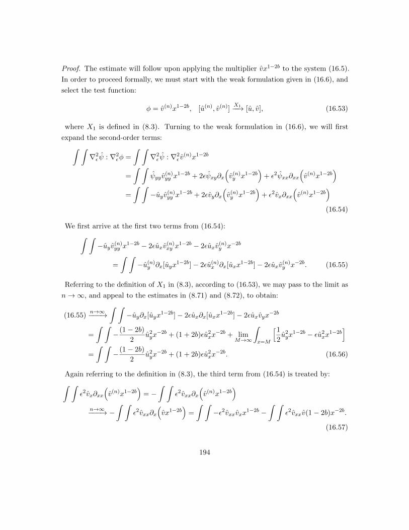
Proof. The estimate will follow upon applying the multiplier vx1−2b to the system (16.5).

In order to proceed formally, we must start with the weak formulation given in (16.6), and

select the test function:

φ = v(n)x1−2b, [u(n), v(n)]X1−−→ [u, v], (16.53)

where X1 is defined in (8.3). Turning to the weak formulation in (16.6), we will first

expand the second-order terms:∫ ∫∇2ε ψ : ∇2

εφ =

∫ ∫∇2ε ψ : ∇2

ε v(n)x1−2b

=

∫ ∫ψyyv

(n)yy x

1−2b + 2εψxy∂x

(v(n)y x1−2b

)+ ε2ψxx∂xx

(v(n)x1−2b

)=

∫ ∫−uyv(n)

yy x1−2b + 2εvy∂x

(v(n)y x1−2b

)+ ε2vx∂xx

(v(n)x1−2b

)(16.54)

We first arrive at the first two terms from (16.54):∫ ∫−uyv(n)

yy x1−2b − 2εuxv

(n)xy x

1−2b − 2εuxv(n)y x−2b

=

∫ ∫−u(n)

y ∂x[uyx1−2b]− 2εu(n)

x ∂x[uxx1−2b]− 2εuxv

(n)y x−2b. (16.55)

Referring to the definition of X1 in (8.3), according to (16.53), we may pass to the limit as

n→∞, and appeal to the estimates in (8.71) and (8.72), to obtain:

(16.55)n→∞−−−→

∫ ∫−uy∂x[uyx

1−2b]− 2εux∂x[uxx1−2b]− 2εuxvyx

−2b

=

∫ ∫−(1− 2b)

2u2yx−2b + (1 + 2b)εu2

xx−2b + lim

M→∞

∫x=M

[1

2u2yx

1−2b − εu2xx

1−2b]

=

∫ ∫−(1− 2b)

2u2yx−2b + (1 + 2b)εu2

xx−2b. (16.56)

Again referring to the definition in (8.3), the third term from (16.54) is treated by:∫ ∫ε2vx∂xx

(v(n)x1−2b

)= −

∫ ∫ε2vxx∂x

(v(n)x1−2b

)n→∞−−−→ −

∫ ∫ε2vxx∂x

(vx1−2b

)=

∫ ∫−ε2vxxvxx1−2b −

∫ ∫ε2vxxv(1− 2b)x−2b.

(16.57)

194

Integrating by parts the first term on the right-hand side of (16.57), and appealing to

estimate (8.72):∫ ∫−ε2vxxvxx1−2b =

∫ ∫ε2

1− 2b

2|vx|2x−2b − lim

M→∞

∫x=M

ε2

2v2xx

1−2b

=

∫ ∫ε2

1− 2b

2|vx|2x−2b. (16.58)

Integrating by parts the second term on the right-hand side of (16.57), and again appealing

to estimates (8.71) - (8.73) for the M -limit below:

−∫ ∫

ε2vxxv(1− 2b)x−2b =

∫ ∫ε2(1− 2b)vx∂x

[vx−2b

]+ limM→∞

∫x=M

ε2(1− 2b)vxvx−2b

=

∫ ∫ε2(1− 2b)v2

xx−2b −

∫ ∫ε22b(1− 2b)vxvx

−2b−1

=

∫ ∫ε2(1− 2b)v2

xx−2b +

∫ ∫ε2b(1− 2b)v2∂xx

−2b−1

− limM→∞

ε2b(1− 2b)v2x−2b−1

=

∫ ∫ε2(1− 2b)v2

xx−2b −

∫ ∫ε2b(1− 2b)(2b+ 1)v2x−2b−2.

(16.59)

Combining the above estimates:

(16.57) =

∫ ∫3

2(1− 2b)ε2v2

xx−2b − b(2b+ 1)(1− 2b)ε2v2x−2b−2. (16.60)

Hence, summarizing (16.55) - (16.59):

| limn→∞

∫ ∫∇2ε ψ : ∇2

εφ| = |∫ ∫

∇2ε ψ : ∇2

ε (vx1−2b)| .

∫ ∫[ε2v2

x + εu2x + u2

y]x−2b. (16.61)

We will now turn to the profile terms from Su, which upon consultation with (16.6), the

definition in (8.3), and (16.53), read:∫ ∫ [uRux + uRxu+ uRyv + vRuy

]· u(n)

x x1−2b

n→∞−−−→∫ ∫ [

uRux + uRxu+ uRyv + vRuy

]· uxx1−2b. (16.62)

We now turn our attention to (16.62). The first term yields the desired positivity:∫ ∫uRu

2xx

1−2b & minuR

∫ ∫u2xx

1−2b. (16.63)

195

Next, by (2.12), (2.18):

|∫ ∫

uRxuuxx1−2b| ≤ ||uRxx||L∞ ||uxx

12−b||L2 ||ux−

12−b||L2

≤ O(δ)||uxx12−b||2L2 . (16.64)

Next, we shall split uR = uPR + uER, and use estimate (2.14) and (2.16) for (16.65) below

and (2.18) for (16.66) below:

|∫ ∫

uPRyvuxx1−2b| ≤ ||yuPRy||L∞ ||vyx

12−b||2L2 , (16.65)

|∫ ∫ √

εuERY vuxx1−2b| ≤ ||uERY x

32 ||L∞ ||

√εvx−

12−b||L2 ||uxx

12−b||L2

.√ε[||√εvx−

12−b||2L2 + ||uxx

12−b||2L2

]. (16.66)

For the fourth term from (16.62), by estimates (2.10) and (2.20):

|∫ ∫

vRuyuxx1−2b| ≤ ||vRx

12 ||L∞ ||uyx−b||L2 ||uxx

12−b||L2

≤ O(δ)||uyx−b||L2 ||uxx12−b||L2 . (16.67)

Summarizing the last four calculations:

|(16.62)| &∫ ∫

u2xx

1−2b −O(δ)[||ux−

12−b||2L2

+ ||uyx−b||2L2 + ||√εvx−

12−b||2L2

]. (16.68)

The final three terms appearing on the right-hand side above all appear on the right-hand

side of estimate (16.52). Turning now to the profile terms, from Sv, for which we read (16.6)

with φ = v(n)x1−2b, appeal to (8.3) and (16.53), giving ultimately:∫ ∫ε[uRvx + vRxu+ vRvy + vRyv

]· ∂x[v(n)x1−2b]

n→∞−−−→∫ ∫

ε[uRvx + vRxu+ vRvy + vRyv

]· ∂x[vx1−2b]. (16.69)

We will treat each term in (16.69). For the first term from (16.69):∫ ∫εuRvx

(vxx

1−2b + (1− 2b)vx−2b)

=

∫ ∫εuRv

2xx

1−2b + b(1− 2b)uRεv2x−1−2b −

∫ ∫1− 2b

2εuRxv

2x−2b

196

&∫ ∫

εv2xx

1−2b + b

∫ ∫εv2x−1−2b. (16.70)

Above we have used (2.12) and (2.18). For the second term, we integrate by parts:∫ ∫εvRxu∂x[vx1−2b] =

∫ ∫−ε∂x

(vRxu

)· vx1−2b + lim

M→∞

∫x=M

vRxuvx1−2b

=

∫ ∫−εvRxxuvx1−2b − εvRxvuxx1−2b

≤√ε||vRxx

32 , vRxxx

52 ||L∞

[||ux−

12−b||2L2

+ ||uxx12−b||2L2 + ||

√εvx−

12−b||2L2

]. (16.71)

The above M−limit vanishes according to estimates (8.71), and we have used estimates

(2.8) and (2.17). For the third term, we recall estimates (2.10), (2.20):∫ ∫εvRvyvxx

1−2b + c0εvRvyvx−2b

≤√ε||vRx

12 ||L∞

[||vyx

12−b||2L2 + ||

√εvxx

12−b||2L2 + ||

√εvx−

12−b||2L2

]. (16.72)

For the fourth term, we integrate by parts and appeal to (8.71), (2.8) - (2.10), and (2.17):∫ ∫εvRyv · ∂x[vx1−2b] = −

∫ ∫ε∂x[vRyv] · vx1−2b + lim

M→∞

∫x=M

εvRyv2x1−2b

=

∫ ∫−εvRxyv2x1−2b − εvRyvxvx1−2b

≤ ||vRyx, vRxyx2||L∞[||√εvxx

12−b||2L2 + ||

√εvx−

12−b||2L2

]. (16.73)

Summarizing these four terms,

|(16.69)| &∫ ∫

εv2xx

1−2b + b

∫ ∫εv2x−1−2b

−O(δ)[||ux−

12−b, uxx

12−b||2L2 + ||

√εvx−

12−b,√εvxx

12−b||2L2

]. (16.74)

On the right-hand side, appealing again to (8.3), (16.53), and the definitions of f , g in

(16.2) - (16.3), one obtains:∫ ∫f u(n)

x x1−2b + g[v(n)x x1−2b + (1− 2b)v(n)x−2b

]n→∞−−−→

∫ ∫f uxx

1−2b + g[vxx

1−2b + (1− 2b)vx−2b], (16.75)

Placing the above estimates together yields the estimate (16.52).

197

We will now introduce some notation, which is a natural adaptation of what is found in

Section 8 to the weaker weight of x−b. The reader should recall the definitions of the cutoff

functions introduced in (8.1) - (8.2). The energy norms are defined as follows:

||u, v||2X1,b:= ||uyx−b||2L2 + ||

√εvx, vyx

12−b||2L2 (16.76)

||u, v||2X2,b:= ||uxy · ρ2x

1−b||2L2 + ||√εvxx, vxy · ρ

322 x

32−b||2L2 , (16.77)

||u, v||2X3,b:= ||uxxy · ρ2

3x2−b||2L2 + ||

√εvxxx, vxxy · ρ

523 x

52−b||2L2 . (16.78)

Definition 16.3. The norms Y2,b, Y3,b are strengthenings of X2,b, X3,b near the boundary,

x = 1, and defined through:

||u, v||2Y2,b := ||uxyx1−b||2L2 + ||√εvxx, vxyx

32−b||2L2 + ||uyy||L2(x≤2000), (16.79)

||u, v||2Y3,b := ||uxxy · ζ3x2−b||2L2 + ||

√εvxxx, vxxy · ζ3x

52−b||2L2 . (16.80)

Definition 16.4. The norm Zb is defined through:

||u, v||Zb :=||u, v||X1,b∩X2,b∩X3,b+ εN2 ||u, v||Y2,b + εN3 ||u, v||Y3,b

+ εN4 ||ux14−b,√εvx

12−b||L∞ + εN5 sup

x≥20||√εvxx

32−b, uxx

54−b||L∞

+ εN6 supx≥20||uyx

12−b||L2

y+ εN7

[ ∫ ∞20

x4−b||√εvxx||2L∞y dx

] 12. (16.81)

Next, we record the second and third order versions of the energy and positivity estimates,

which mimic Propositions 9.8, 9.13, 9.16, 9.18. We will omit most details, and record only

those differences which arise.

Lemma 16.5 (Second-Order Energy Estimate). Fix any 0 < b < 1. Let δ, ε be sufficiently

small relative to universal constants, and ε << δ. Then for [u, v] ∈ Z solutions to (16.2) -

(16.3):

||uxyρ2x1−b||2L2 . O(δ)||

√εvxx, vxyρ

322 x

32−b||2L2 + ||u, v||2X1,b

+W1,b +W2,E,b, (16.82)

where (recall the definition of ρ2 from (8.2)):

W2,E,b :=

∫ ∫fxuxρ

22x

2−2b +

∫ ∫εgxvxρ

22x

2−2b, (16.83)

W2,P,b =

∫ ∫fxuxxρ

32x

3−2b +

∫ ∫εgxvxxρ

32x

3−2b, (16.84)

W2,b :=W2,E,b +W2,P,b. (16.85)

198

Proof. Differentiating the weak formulation gives:∫ ∫∇2ε ψx : ∇2

εφ−∫ ∫

∂xSu(u, v) · φy + ε∂xSv(u, v) · φx

=

∫ ∫εn2

+γ[− ∂xfφy + ε∂xgφx

], (16.86)

For the second-order energy estimate, we select φ = ρ22v

(n)x2−2b, where:

[u(n), v(n)] ∈ C∞0,D, [u(n), v(n)]X1−−→ [u, v]. (16.87)

Let us turn to the highest-order terms:∫ ∫∇2ε ψx : ∇2

εφ =

∫ ∫∇2ε v : ∇2

ερ22v

(n)x2−2b

=

∫ ∫vyyρ

22v

(n)yy x

2−2b + 2εvxy∂x[v(n)y ρ2

2x2−2b] + ε2vxx∂xx[ρ2

2v(n)x2−2b]

=

∫ ∫uxyρ

22u

(n)xy x

2−2b + 2εvxy∂x[v(n)y ρ2

2x2−2b] + ε2vxx∂xx[ρ2

2v(n)x2−2b]

=

∫ ∫−∂x[uxyρ

22x

2−2b]u(n)y − 2εvxxyv

(n)y ρ2

2x2−2b − ε2vxxx∂x[ρ2

2v(n)x2−2b]

(16.88)

One now checks according to the definition (8.3), that (16.87) suffices to pass to the limit

in the above identity, which upon integrating by parts in x yields:

(16.88)n→∞−−−→

∫ ∫−∂x[uxyρ

22x

2−2b]uy − 2εvxxyvyρ22x

2−2b − ε2vxxx∂x[ρ22vx

2−2b]

=

∫ ∫[u2xy + εu2

xx + ε2v2xx]ρ2

2x2−2b + J.

where |J | = |c0ε2v2x∂xx(ρ2

2x2−2b) + c1ε

2v2∂4x(ρ2

2x2−2b)| . ||u, v||2X1,b

. From here, repeating

the calculations in Proposition 9.8 gives the desired result, where the required integrations

by parts are justified upon using that b > 0, combined with the estimates in (8.71) - (8.73).

These justifications are analogous to those in Lemma 16.1, and so we omit the details.

Lemma 16.6 (Second-Order Positivity Estimate). Fix any 0 < b < 1. Let δ, ε be sufficiently

small relative to universal constants, and ε << δ. Then for [u, v] ∈ Z solutions to (16.2) -

(16.3):

||√εvxx, vxyρ

322 x

32−b||2L2 . ||uxyρ2x

1−b||2L2 + ||u, v||2X1,b+W1,b +W2,b. (16.89)

199

Proof. We start again with the weak formulation in (16.86). Fix a large 0 < L <∞. We

then make the selection: φ = v(n)x · ρ3

2x3−2bL , where, referring to (9.168), the weight xL is

defined via: xL :=(aL ∗ φL

)χ(

x10L

). Define the domain: ΩL := x : 3 < x < 50L+ 100,

so that vx · ρ32x

3−2bL = 0 on ΩC

L . The sequence v(n) is selected according to:

[u(n)x , v(n)

x ] ∈ C∞0,D(ΩL), [u(n)x , v(n)

x ]H1(ΩL)−−−−−→ [ux, vx]. (16.90)

The existence of such a sequence is guaranteed due to the standard Sobolev space theory,

because we are now in the un-weighted setting. It is now straightforward to repeat all

estimates in Proposition 9.13 using the test function φ. Upon doing so, we pass to the limit

first as n→∞, and then as L→∞ to obtain the desired estimate.

Lemma 16.7 (Third-Order Energy Estimate). Fix any 0 < b < 1. Let δ, ε be sufficiently

small relative to universal constants, and ε << δ. Then for [u, v] ∈ Z solutions to (16.2) -

(16.3):

||uxxyρ23x

2−b||2L2 . O(δ)||√εvxxx, vxxyρ

523 x

52−b||2L2 + ||u, v||2X1,b∩X2,b

+2∑i=1

Wi,b +W3,E,b,

(16.91)

where

W3,E,b :=

∫ ∫fxxuxxρ

43x

4−2b +

∫ ∫εgxxvxxρ

43x

4−2b, (16.92)

W3,P,b :=

∫ ∫fxxuxxxρ

53x

5−2b +

∫ ∫εgxxvxxxρ

53x

5−2b, (16.93)

W3,b := W3,E,b +W3,P,b. (16.94)

Proof. The first step is to differentiate the weak formulation (16.86) yet again, which

formally takes place using difference quotients, yielding:∫ ∫∇2ε ψxx : ∇2

εφ−∫ ∫

∂xxSu(u, v) · φy + ε∂xxSv(u, v) · φx

=

∫ ∫εn2

+γ[− ∂xxfφy + ε∂xxgφx

], (16.95)

Fix any L large, finite. The selection of test function is now φ := v(n)x ρ4

3x4−2bL , where the

sequence:

[u(n)xx , v

(n)xx ] ∈ C∞0,D(ΩL), [u(n)

xx , v(n)xx ]

H1(ΩL)−−−−−→ [uxx, vxx]. (16.96)

200

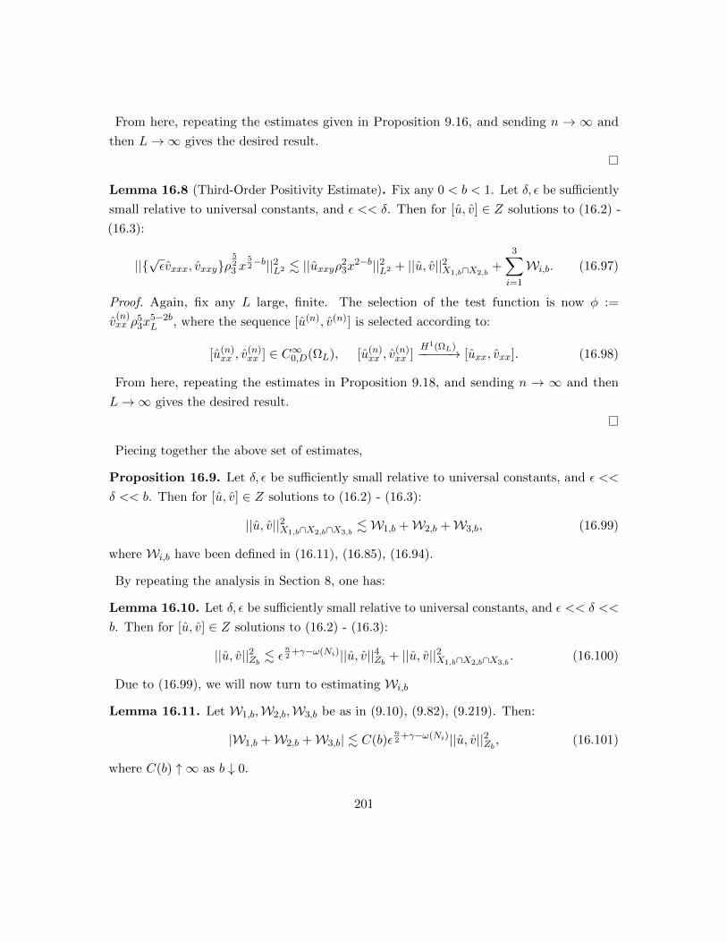
From here, repeating the estimates given in Proposition 9.16, and sending n → ∞ and

then L→∞ gives the desired result.

Lemma 16.8 (Third-Order Positivity Estimate). Fix any 0 < b < 1. Let δ, ε be sufficiently

small relative to universal constants, and ε << δ. Then for [u, v] ∈ Z solutions to (16.2) -

(16.3):

||√εvxxx, vxxyρ

523 x

52−b||2L2 . ||uxxyρ2

3x2−b||2L2 + ||u, v||2X1,b∩X2,b

+3∑i=1

Wi,b. (16.97)

Proof. Again, fix any L large, finite. The selection of the test function is now φ :=

v(n)xx ρ5

3x5−2bL , where the sequence [u(n), v(n)] is selected according to:

[u(n)xx , v

(n)xx ] ∈ C∞0,D(ΩL), [u(n)

xx , v(n)xx ]

H1(ΩL)−−−−−→ [uxx, vxx]. (16.98)

From here, repeating the estimates in Proposition 9.18, and sending n → ∞ and then

L→∞ gives the desired result.

Piecing together the above set of estimates,

Proposition 16.9. Let δ, ε be sufficiently small relative to universal constants, and ε <<

δ << b. Then for [u, v] ∈ Z solutions to (16.2) - (16.3):

||u, v||2X1,b∩X2,b∩X3,b.W1,b +W2,b +W3,b, (16.99)

where Wi,b have been defined in (16.11), (16.85), (16.94).

By repeating the analysis in Section 8, one has:

Lemma 16.10. Let δ, ε be sufficiently small relative to universal constants, and ε << δ <<

b. Then for [u, v] ∈ Z solutions to (16.2) - (16.3):

||u, v||2Zb . εn2

+γ−ω(Ni)||u, v||4Zb + ||u, v||2X1,b∩X2,b∩X3,b. (16.100)

Due to (16.99), we will now turn to estimating Wi,b

Lemma 16.11. Let W1,b,W2,b,W3,b be as in (9.10), (9.82), (9.219). Then:

|W1,b +W2,b +W3,b| . C(b)εn2

+γ−ω(Ni)||u, v||2Zb , (16.101)

where C(b) ↑ ∞ as b ↓ 0.

201

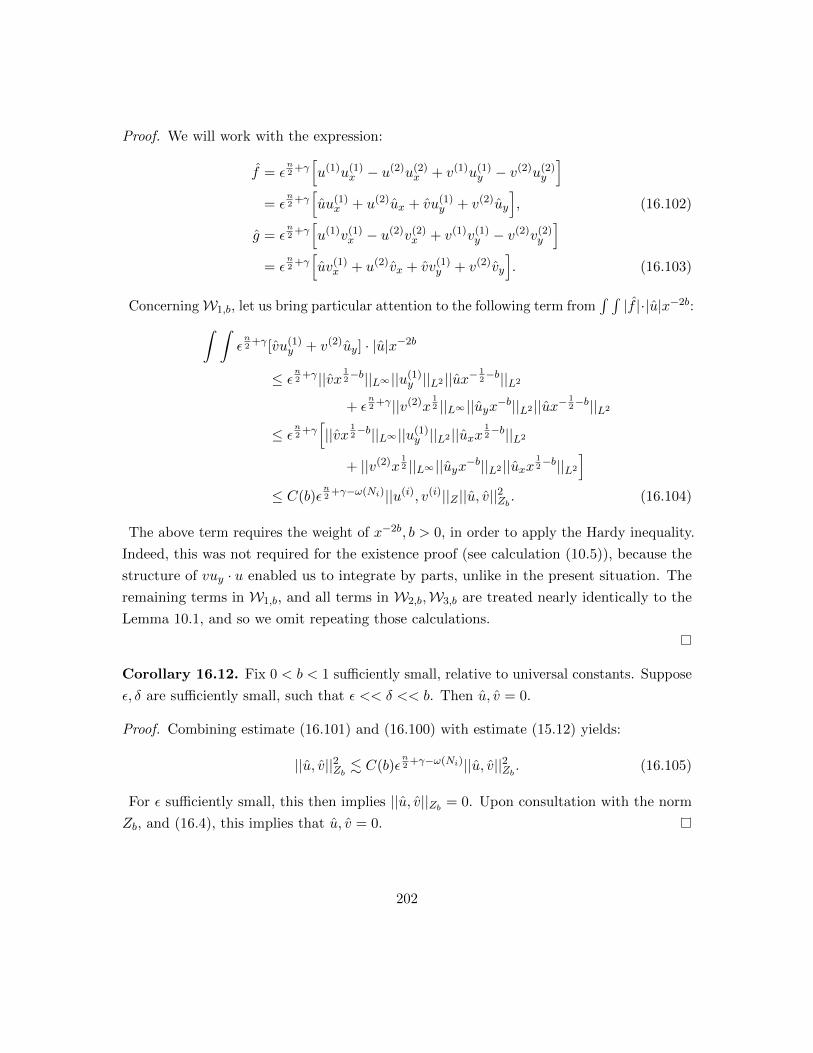
Proof. We will work with the expression:

f = εn2

+γ[u(1)u(1)

x − u(2)u(2)x + v(1)u(1)

y − v(2)u(2)y

]= ε

n2

+γ[uu(1)

x + u(2)ux + vu(1)y + v(2)uy

], (16.102)

g = εn2

+γ[u(1)v(1)

x − u(2)v(2)x + v(1)v(1)

y − v(2)v(2)y

]= ε

n2

+γ[uv(1)

x + u(2)vx + vv(1)y + v(2)vy

]. (16.103)

ConcerningW1,b, let us bring particular attention to the following term from∫ ∫|f |·|u|x−2b:∫ ∫

εn2

+γ [vu(1)y + v(2)uy] · |u|x−2b

≤ εn2

+γ ||vx12−b||L∞ ||u(1)

y ||L2 ||ux−12−b||L2

+ εn2

+γ ||v(2)x12 ||L∞ ||uyx−b||L2 ||ux−

12−b||L2

≤ εn2

+γ[||vx

12−b||L∞ ||u(1)

y ||L2 ||uxx12−b||L2

+ ||v(2)x12 ||L∞ ||uyx−b||L2 ||uxx

12−b||L2

]≤ C(b)ε

n2

+γ−ω(Ni)||u(i), v(i)||Z ||u, v||2Zb . (16.104)

The above term requires the weight of x−2b, b > 0, in order to apply the Hardy inequality.

Indeed, this was not required for the existence proof (see calculation (10.5)), because the

structure of vuy · u enabled us to integrate by parts, unlike in the present situation. The

remaining terms in W1,b, and all terms in W2,b,W3,b are treated nearly identically to the

Lemma 10.1, and so we omit repeating those calculations.

Corollary 16.12. Fix 0 < b < 1 sufficiently small, relative to universal constants. Suppose

ε, δ are sufficiently small, such that ε << δ << b. Then u, v = 0.

Proof. Combining estimate (16.101) and (16.100) with estimate (15.12) yields:

||u, v||2Zb . C(b)εn2

+γ−ω(Ni)||u, v||2Zb . (16.105)

For ε sufficiently small, this then implies ||u, v||Zb = 0. Upon consultation with the norm

Zb, and (16.4), this implies that u, v = 0.

202

Remark 16.13. We have controlled the second and third order energy norms, (16.77) -

(16.78) in order to treat the term∫ ∫

vu(1)y |u|x−2b, which appears in (16.104). This term

forces us to control ||vx12−b||L∞ . One cannot get around placing this term in L∞ (for

instance by integrating by parts from u(1)y ) because this produces suboptimal decay rates,

according to (8.92) - (8.93).

This then establishes Theorem 11.1, and controlling [u, v] ∈ Z then immediately establishes

the main result, Theorem 1.2.

Acknowledgements: The author thanks Yan Guo for many valuable discussions regard-

ing this research. The author also thanks Bjorn Sandstede for introducing him to the paper

[BKL94].

References

[Ad03] R. Adams, J. Fournier, Sobolev Spaces. Second Edition, Elsevier Science Ltd,

Kidlington, Oxford, (2003).

[AWXY15] R. Alexandre, Y.-G. Wang, C.-J. Xu, T. Yang, Well-posedness of the Prandtl

equation in Sobolev spaces. Journal of the American Mathematical Society, Volume

28, Number 3, (2015), P. 745-784.

[As91] A. Asano, Zero viscosity limit of incompressible Navier-Stokes equations, Conference

at the Fourth Workshop on Mathematical Aspects of Fluid and Plasma Dynamics,

Kyoto, 1991.

[BR80] H. Blum, R. Rannacher, On the Boundary Value Problem of the Biharmonic

Operator on Domains with Angular Corners, Math. Meth. in the Appl. Sci., (1980),

556-581.

[BKL94] J. Bricmont, A. Kupiainen, G. Lin. Renormalization Group and Asymptotics of

Solutions of Nonlinear Parabolic Equations. Comm. Pure. Appl. Math., 47, (1994),

893-922.

[DM15] A.L. Dalibard, and N. Masmoudi “Phenomene de separation pour l’equation de

Prandtl stationnaire.” Seminaire Laurent Schwartz - EDP et applications (2014-2015):

1-18.

203

[DPV12] E. Di Nezza, G. Palatucci, E. Valdinoci. Hitchhiker’s guide to fractional Sobolev

spaces, Bulletin des Sciences Mathematiques, 136 (2012).

[ZD94] Z. Ding. A proof of the trace theorem of Sobolev spaces on Lipschitz domains. Proc.

Amer. Math. Soc., 124, Number 2, (1996), 591-600.

[E00] W. E, Boundary layer theory and the zero-viscosity limit of the Navier-Stokes equation.

Acta Math. Sin. (Engl. Ser.) 16, 2 (2000), P. 207-218.

[EE97] W. E, and B. Engquist. Blowup of solutions of the unsteady Prandtl’s equation.

Comm. Pure Appl. Math., 50, 12 (1997), P. 1287-1293.

[EV10] L.C. Evans, Partial Differential Equations. Second Edition. Graduate Studies in

Mathematics. American Mathematical Society, Providence, RI, (2010).

[Galdi11] G.P. Galdi, An Introduction to the Mathematical Theory of the Navier-Stokes

Equations. Second Edition. Springer Monographs in Mathematics. (2011).

[GVD10] D. Gerard-Varet and E. Dormy. On the ill-posedness of the Prandtl equation.

Journal of the American Mathematical Society, Volume 23, Number 2, (2010), P.

591-609.

[GVMM16] D. Gerard-Varet, Y. Maekawa, and N. Masmoudi. Gevrey stability of Prandtl

expansions for 2D Navier-Stokes flows. arXiv preprint 1607.06434v1, (2016).

[GVM13] D. Gerard-Varet and N. Masmoudi. Well-posedness for the Prandtl system without

analyticity or monotonicity. arXiv preprint 1305.0221v1, (2013).

[GVN12] D. Gerard-Varet and T. Nguyen, Remarks on the ill-posedness of the Prandtl

equation. Asymptotic Analysis, 77, no.1-2, P. 71-88, (2012).

[GJT16] G-M. Gie, C-Y. Jung, and R. Temam, Recent Progresses in the Boundary Layer

Theory. Disc. Cont. Dyn. Syst. A, 36, 5 (2016), P. 2521 - 2583.

[Gr11] P. Grisvard. Elliptic Problems in Nonsmooth Domains. Classics in Applied Mathe-

matics. SIAM, (2011).

[Gre00] E. Grenier. On the nonlinear instability of Euler and Prandtl equations. Comm.

Pure Appl. Math. 53, 9 (2000), P. 1067-1091.

204

[GGN15a] E. Grenier, Y. Guo, T. Nguyen, Spectral instability of symmetric shear flows in

a two-dimensional channel, To appear: Adv. Math.

[GGN15b] E. Grenier, Y. Guo, T. Nguyen, Spectral instability of characteristic boundary

layer flows. To appear: Duke Math. J.

[GGN15c] E. Grenier, Y. Guo, T. Nguyen, Spectral instability of Prandtl boundary layers:

an overview. Analysis (Berlin), 35, no.4, (2015), P. 343-355.

[GN14] Y. Guo, and T. Nguyen. Prandtl boundary layer expansions of steady Navier-Stokes

flows over a moving plate. arXiv preprint 1411.6984, (2014).

[GN11] Y. Guo and T. Nguyen. A note on the Prandtl boundary layers. Comm. Pure Appl.

Math., 64 (2011), no. 10, P. 1416-1438.

[HH03] L. Hong and J. Hunter. Singularity formation and instability in the unsteady

inviscid and viscous Prandtl equations. Comm. Math. Sci. Vol. 1, No. 2, P. 293-316.

[IV16] M. Ignatova and V. Vicol. Almost Global Existence for the Prandtl Boundary Layer

Equations. Arch. Rational Mech. Anal., 220, (2016) P. 809-848.

[Iy15] S. Iyer. Steady Prandtl Boundary Layer Expansion of Navier-Stokes Flows over a

Rotating Disk. arXiv preprint 1508.06956v2, (2015).

[Ka84] T. Kato. Remarks on zero viscosity limit for nonstationary Navier-Stokes flows with

boundary. Seminar on nonlinear partial differential equations (Berkeley, Calif., 1983),

85-98. Math. Sci. Res. Inst. Publ., 2. Springer, New York - Berlin, 1984.

[KMVW14] I. Kukavica, N. Masmoudi, V. Vicol, T.K. Wong, On the local well-posedness

of the Prandtl and Hydrostatic Euler equations with multiple monotonicity regions.

SIAM Journal of Mathematical Analysis., Vol. 46, No. 6, P. 3865-3890.

[KV13] I. Kukavica and V. Vicol, On the local existence of analytic solutions to the Prandtl

boundary layer equations. Commun. Math. Sci., 11(1), (2013), P. 269-292.

[KVW15] I. Kukavica, V. Vicol, F. Wang, The van Dommelen and Shen singularity in the

Prandtl equations. arXiv preprint 1512.07358v1, (2015).

[KC04] P. Kundu and I Cohen, Fluid Mechanics. Third Edition. Elsevier Academic Press.

(2004).

205

[LCS03] M. C. Lombardo, M. Cannone and M. Sammartino, Well-posedness of the boundary

layer equations, SIAM J. Math. Anal. 35(4), P. 987-1004, 2003.

[Mae14] Y. Maekawa, On the inviscid problem of the vorticity equations for viscous incom-

pressible flows in the half-plane, Comm. Pure. Appl. Math., 67, (2014), 1045-1128.

[MW15] N. Masmoudi and T.K. Wong, Local in time existence and uniqueness of solutions

to the Prandtl equations by energy methods, Comm. Pure. Appl. Math., 68, (2015),

1683-1741.

[MT08] A. Mazzucato and M. Taylor. Vanishing viscocity plane parallel channel flow and

related singular perturbation problems. Anal. PDE, 1 (1); 35-93 (2008).

[NI59] L. Nirenberg. On elliptic partial differential equations. Annali Della Scoula Normale

Superiore Di Pisa., 1959.

[OS99] Oleinik, O.A. and Samokhin , V.N, Mathematical models in boundary layer theory.

Applied Mathematics and Mathematical Computation, 15. Champan and Hall/ CRC,

Boca Raton, FL, 1999.

[Ol67] O.A. Oleinik. On the mathematical theory of boundary layer for an unsteady flow

of incompressible fluid. J. Appl. Math. Mech., 30, (1967), P. 951-974.

[Orlt98] M. Orlt, Regularity for Navier-Stokes in domains with corners, Ph.D. Thesis, 1998

(in German).

[OS93] M. Orlt, and A.M. Sandig, Regularity of viscous Navier-Stokes flows in non smooth

domains. Boundary value problems and integral equations in non smooth domains

(Luminy, 1993). Lecture Notes in Pure and Appl. Math., 167, Dekker, New York, 1995.

[Pr1905] L. Prandtl, Uber flussigkeits-bewegung bei sehr kleiner reibung. In Verhandlungen

des III Internationalen Mathematiker-Kongresses, Heidelberg. Teubner, Leipzig, 1904,

pp. 484 - 491.

English Translation: “Motion of fluids with very little viscosity,” Technical Memoran-

dum No. 452 by National Advisory Committee for Aeuronautics.

[SC98] M. Sammartino and R. Caflisch, Zero viscosity limit for analytic solutions of the

Navier-Stokes equation on a half-space. I. Existence for Euler and Prandtl equations.

Comm. Math. Phys. 192 (1998), no. 2, 433-461.

206

[SC98] M. Sammartino and R. Caflisch, Zero viscosity limit for analytic solutions of the

Navier-Stokes equation on a half-space. II. Construction of the Navier-Stokes soution.

Comm. Math. Phys. 192 (1998), no. 2, 463 - 491.

[Ser66] J. Serrin, Asymptotic behaviour of velocity profiles in the Prandtl boundary layer

theory. Proc. R. Soc. Lond. A, 299, 491-507, (1967).

[Sch00] Schlichting, H and Gersten, K. Boundary Layer Theory. 8th edition, Springer-Verlag

2000.

[ST93] E. Stein, Harmonic Analysis: Real Variable Methods, Orthogonality, and Oscillatory

Integrals. Second Edition. Princeton University Press, Princeton NJ, (1993).

[XZ04] Z. Xin and L. Zhang, On the global existence of solutions to the Prandtl’s system.

Adv. Math., Volume 181, Issue 1, (2004), P. 88-133.

207