Saliva Diagnostics for Kidney Disease

Project Report

Linden Heflin and Sarah Walsh

Submitted to Dr. Miguel Bagajewicz

April 30, 2007

1

TABLE OF CONTENTS

ABSTRACT 2

INTRODUCTION 3

SALIVA 4

SCREENING PROCEDURE 5

Procedure Flow Chart 6

THE KIDNEY 7

CREATININE AND GFR 8

Kidney Disease Stages 9

THE TEST & KIT 10

FDA APPROVAL 11

PRICING MODEL 12

AWARENESS FUNCTION 13

CONSUMER PREFERENCE MODEL 15

Discomfort 16

Sensitivity 16

False Negative Rate 19

False Positive Rate 24

CONSUMER SATISFACTION MODEL 27

CONSUMER PREFERENCE 28

PRODUCT DESIGN 30

DEMAND 31

NET PRESENT WORTH 34

CONCLUSION 36

REFERENCES 37

2

ABSTRACT

This project evaluates the development of a saliva-based diagnostic tool analyzing kidney functioning by measuring the concentration of creatinine, a biomarker related to blood filtration. An economic analysis reveals a high expected demand and profitability for this product in comparison to existing blood tests that are currently being used in the medical community. The test utilizes a reaction between creatinine and picric acid which results in a color change that can be used to determine the concentration of creatinine and therefore the level of kidney functioning. Some compounds, however, are known to interfere with this reaction, creating misleading results. Various product designs were developed in response to this issue, such as adding certain components to the test to reduce or monitor the affects of the interfering compounds. A consumer satisfaction model was created to determine consumer preference with regard to discomfort level, early diagnosis efficacy, and the likelihood of false results due to interfering compounds. A price and demand model, including consumer preference, as well as consumer knowledge and competition, found that the highest demand was for a product designed to reduce negatively interfering compounds while monitoring the level of positively interfering compounds. However the product cost associated with that design option was significantly higher than others. A net present worth calculation was used to determine the most profitable product design which estimated an NPW of $10 million for a design priced at $4/test which reduces negative interference, but does not monitor levels of positively interfering compounds.

3

INTRODUCTION

Medical diagnosis currently depends heavily on information gathered from blood

tests, urine tests, biopsies, and physical examination. Saliva remains a largely

untapped source of medical information that can enhance diagnosis accuracy

while saving the patient from some of the discomfort associated with a blood test

or other more invasive procedures. Many of blood’s constituents make their way

into saliva, thus making saliva an indicator of the current state of the blood and

the rest of the body. Many biomarkers, or substances used as indicators of

biological states, can be readily found in saliva.

The specific goal identified through this project is a salivary diagnostic tool of the

kidney. A creatinine clearance test is a typical assay performed upon admittance

in order to assess the overall health of a patient. Kidney malfunction can indicate

many other systemic problems, therefore a fast, effective, inexpensive, and

noninvasive creatinine clearance test would be very beneficial.

The kidney produces urine mainly through passive diffusion, which is the main

mechanism at work in the formation of saliva1. Therefore, items leaving the

blood in the kidneys should be similar to those leaving the blood at the salivary

glands. When a physician orders a creatinine clearance test, he is looking for the

concentration of creatinine in the blood. The smaller the concentration is, the

healthier the kidney is because it is sufficiently removing creatinine from the

blood. Because of the parallels between blood and saliva, a creatinine clearance

test performed on saliva should provide this same information, but faster and with

less discomfort to the patient.

4

SALIVA

Saliva is composed of many compounds. Saliva is 98% water with some mucus

and a wide variety of electrolytes. A detailed list of the compounds found in

saliva is given in Table 1, below.

Table 1: Components of Saliva2,5,14

Electrolytes Concentration Mucus Concentration

Sodium 32 mmol/L Mucopolysaccharides

Potassium 22 mmol/L Glucose 175 umol/L

Calcium 1.7 mmol/L Metabolites

Magnesium 0.18 mmol/L Bilirubin 15 umol/L

Copper 0.4 mmol/L α-ketoglutaric acid 2.4 umol/L

Lead 0.55 mmol/L Pyruvic acid 75 umol/L

Cobalt 1.2 mmol/L Proteins

Strontium 1 umol/L α-amylase 650-800 ug/ml

Hydrogen Carbonate 20 mmol/L Peroxidase 5-6 ug/ml

Iodide 10 umol/L Secretory IgA 96-102 ug/ml

Bromide 14 mmol/L Lactoferrin 1-2 ug/ml

Hypothiocyanate 1.2 umol/L Fibronectin 0.2-2 ug/ml

Nitrate 1.1 umol/L Cells 32 mmol/L

Nitrite 178 umol/L

Fluoride 68 umol/L

Sulfate 5.8 umol/L

It has previously been shown that 5 min of rest after eating is sufficient time for a

patient’s mouth to be free of food particles8. A patient with a dry mouth may be

asked to chew inert paraffin gum for up to two minutes to stimulate flow.

Collecting 5mL of saliva is simple and gives a copious amount for a saliva test.

5

SCREENING PROCEDURE FOR VALIDATING THE TEST

Before choosing a salivary creatinine clearance test for this analysis, a screening

procedure was developed in order to choose the best biomarker candidate. The

following questions were asked of each candidate biomarker.

1. Can the biomarker be detected in saliva?

a. What are normal saliva levels for biomarker?

b. How do saliva levels compare to plasma levels?

2. Do abnormal levels indicate threat of organ malfunction or disease?

a. How do we determine baseline concentration?

3. How do you detect abnormal levels?

4. How accurate are detection methods?

5. How widely applicable are detection methods?

a. Are they too specific?

6. How helpful is result in medical decision making?

7. Is test effective in early diagnosis (compared to serum testing)?

a. Does test improve treatment?

b. Does test lead to more cured patients or better managed diseases?

8. Weigh accuracy vs. speed, convenience, portability

9. What is the cost of the detection method?

a. Is test more economical than serum testing?

b. Is it economical enough to be used in the home, or can it only be used in

clinical settings?

This procedure evaluates ideas on all non-economic aspects of the test, from its

accuracy to its actual utility and the usefulness of the information it gives.

However, all of these criteria are related to the profitability of this venture, as will

be discussed in the market analysis.

The screening procedure is also outlined in the following flowchart, Figure 1.

6

Does organ malfunction have salivary biomarkers?

No, back to beginning

Yes, investigate possibility of false negatives

No, back to beginning

Is it accurate enough?

Can it compete with serum tests?

Speed

Patient Comfort

Accuracy Serum tests more desirable

Saliva is superior

Essentially equal

Is it useful for early diagnosis?

Useful as precursor to more invasive tests

No, back to beginning

No, back to beginning

Preliminary Economic Analysis

Not Profitable, back to beginning

Profitable

FDA Pre-Market Notification Figure 1: Screening procedure for salivary

diagnostic test

7

THE KIDNEY

Kidney disease currently afflicts about one in twelve Americans. It is to blame for

about 80,000 deaths per year making it the ninth killer in the country. Also about

a half million Americans depend on dialysis or transplanted kidneys to survive5.

Any diagnostic tool that could catch kidney disease in its early stages can save

these lives and keep people from having to endure dialysis or serious operations.

The kidney’s main responsibility is cleaning the blood of waste. Because urine

forms mainly through passive diffusion, just like saliva, many of blood’s

components exchanged at the kidney are also exchanged at the salivary glands.

Figure 2: The Kidney6

A wide variety of symptoms may call for a kidney test, so physicians call for the

tests quite frequently1. Any of the following problems may call for a diagnostic

test related to the kidney:

8

• High blood pressure

• Fatigue, less energy

• Poor concentration and appetite

• Trouble sleeping and night time muscle cramps

• Swollen feet and ankles

• Puffiness around eyes, particularly in the morning

• Dry, itchy skin

• More frequent urination

Saliva testing can replace the initial blood in these situations. A positive saliva

test may lead to more invasive tests, but a negative one can spare the patient

and physician this inconvenience. When tests indicate elevated creatinine levels,

patients are then usually asked to submit urine tests. For a 24 hour period, the

patient collects and stores all urine they produce and return it for analytical

testing. This allows for a very accurate creatinine measurement since the

quantity is time dependent and is not contingent on other factors such as

hydration.

CREATININE AND GFR

Creatinine, a key in diagnosing kidney disease, is found in both saliva and

plasma. Creatinine is a breakdown product of muscle tissue which the kidney

normally removes from the blood. The following reaction generates creatinine:

Figure 3: Creatinine Formation

Salivary levels of creatinine share a close relationship with serum levels, with an

average concentration 10 times less than serum9:

9

crSPcr 10= (1)

Where Pcr is the plasma creatinine concentration and Scr is the salivary creatinine

concentration.

An elevated creatinine level in the blood suggests kidney malfunction. The

creatinine concentration in the blood is related to the glomerular filtration rate

(GFR). GFR refers to the initial urine formation at the glomerulus. The

glomerulus is a web of capillaries that functions as the first interface between the

blood and the kidney at the Bowman’s capsule. Doctors use GFR most

frequently to identify the stage of kidney disease progression. A healthy pair of

kidneys will have a GFR above 100 mL/min/1.73m2 11. A GFR below 14 is a sign

of end stage kidney failure. Simply put, the GFR is the rate at which toxins are

removed from the body’s blood. Correlations between serum creatinine

concentration and GFR are available, and can be used to develop an equation

relating GFR to salivary creatinine concentration. The following equation is

called the Cockcroft-Gault equation8:

crS

MassAgeGFR

⋅⋅−

=8150

)140( (2)

Where GFR is glomerular filtration rate, mass is in kg, and Scr is the salivary

creatinine concentration in mmol/L.

The following table shows the relationship between GFR and the stages of

kidney disease. The description of the symptoms and the advised treatment is

also given.

10

Table 2: Kidney Disease Stages11

GFR Stage Description Treatment

90+ 1 Normal kidney function Observe, control blood pressure

60-89 2 Mildly reduced kidney function, with urine abnormalities, indicates kidney disease

Find out why kidney function is reduced

30-59 3 Moderately reduced kidney function Make a diagnosis with additional testing

15-29 4 Severely reduced kidney function Plan for end stage renal failure

14 down 5 End stage kidney failure Dialysis and/or transplant

THE TEST

The chemistry used in the creatinine clearance test is the Jaffe Reaction which

involves the combination of picric acid with creatinine to produce a red color13. A

spectrophotometer, which most clinical labs already have, tracks the extent of

reaction by following the intensity of the red color. The assay also requires

NaOH to provide an alkaline environment in which the picrate will form picric

acid, the active compound.

A salivary test has many advantages over a serum test. Because there are no

blood cells in saliva, a saliva sample does not require centrifugation before

testing. The saliva’s ease of collection gives it yet another advantage over serum

testing in that the tools are cheaper and easier to use. Before a patient can give

blood, he must have the area from which the blood is drawn sterilized. The

physician or nurse must then go in with a sterile needle and draw the blood.

Saliva diagnostics requires a less expensive and less invasive vial.

THE KIT

The kit is to contain the following items which make up 10 tests (with their

associated costs in dollars):

11

Table 3: Kit Breakdown

Product Cost per kit $

Test Tubes x10 0.5

Syringes x10 1.5

Box 0.16

Bottle 5.21

Picric Acid 0.875

Sodium Hydroxide 0.875

Creatinine Standard 0.5

Total 9.60

FDA APPROVAL

A salivary diagnostic device falls under the FDA’s regulation. The creatinine

assay would be considered a medical device, which is regulated by the FDA’s

Center for Devices and Radiological Health. The first step in the approval

process is to classify the device. There are three different classifications, each

with differing amounts of approval required. A salivary creatinine test falls into

category II, meaning that Pre-Market Notification is required, but the much more

extensive Pre-Market Approval is not.

The main purpose of Pre-Market Notification is to establish substantial

equivalence. In the case of this device, the test must compare to a blood test

and meet the following requirements:

– Must have the same intended use as the predicate; and

– Must have different technological characteristics and the

information submitted to FDA:

• does not raise new questions of safety and effectiveness;

and

• demonstrates that the device is at least as safe and effective

as the legally marketed device.

12

Other regulations imposed by the FDA are called Good Market Practices or

Quality System Regulation. These criteria must be met, and pertain to issues

such as design, process control, employee training, etc.

PRICING MODEL

A comprehensive pricing model was used to determine the optimal selling price

as well as the combination of product properties which yields the best return.

The most simplified description of this model is illustrated by a classical

microeconomics consumer optimization problem3. This microeconomics model

describes two products, each with a specific demand (d1 and d2 for the new and

old product respectively). The consumer maximizes his satisfaction in the

product subject to the constraints of his budget. This budget constraint can be

described as

Ydpdp 2211 ≤+ (3)

Where p1 is the new product price, p2 is the old product price, and Y is the total

consumer budget.

Many models of consumer utility have been proposed. The function used in this

analysis was the Constant Elasticity of Substitution (CES) utility, given by:

1/ρρ2

ρ121 )d(d)d,u(d += (4)

Where ρ is a constant which sets the elasticity of substitution to a specific value.

For this study, ρ was set to 0.75. Maximizing this utility function yields equation

5.

ρ1

ρ111211 d)dp(Ypdp −−= (5)

13

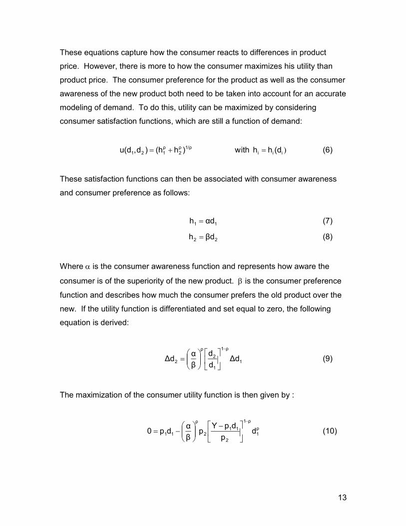
These equations capture how the consumer reacts to differences in product

price. However, there is more to how the consumer maximizes his utility than

product price. The consumer preference for the product as well as the consumer

awareness of the new product both need to be taken into account for an accurate

modeling of demand. To do this, utility can be maximized by considering

consumer satisfaction functions, which are still a function of demand:

)iii1/ρρ

2ρ121 (dhh ith w )h(h)d,u(d =+= (6)

These satisfaction functions can then be associated with consumer awareness

and consumer preference as follows:

11 αdh = (7)

22 βdh = (8)

Where α is the consumer awareness function and represents how aware the

consumer is of the superiority of the new product. β is the consumer preference

function and describes how much the consumer prefers the old product over the

new. If the utility function is differentiated and set equal to zero, the following

equation is derived:

1

ρ1

1

2

ρ

2 ∆dd

d

β

α∆d

−

= (9)

The maximization of the consumer utility function is then given by :

ρ1

ρ1

2

112

ρ

11 dp

dpYp

β

αdp0

−

−

−= (10)

14

This model was used to solve for the demand for various scenarios with different

new product prices, values for α, and values for β.

AWARENESS FUNCTION

The awareness function, denoted by α in equation 7, describes how aware the

consumer is of the superiority of the new product. Awareness is a function of

time, advertising, and professional education. Figure 4 gives an example of how

α varies with time, ultimately reaching a value of one which indicates perfect

knowledge of the new product.

Awareness Function

0

0.2

0.4

0.6

0.8

1

0 1 2 3 4 5

Year

Alpha

Figure 4: Consumer Awareness versus Time

15

Through advertising, α can be shifted to the left, increasing the demand for the

new product. Additionally, actively spreading knowledge of the test to medical

professionals will shift α even further to the left. The following figure represents

the change in α with increased advertising and education.

Awareness Function

0

0.2

0.4

0.6

0.8

1

0 1 2 3 4 5

Year

Alpha

Figure 5: Expected Change in α with Advertising and Education

Advertising, Education

16

CONSUMER PREFERENCE MODEL

To use the pricing model developed previously, a function for β (the consumer

preference function) was developed. β is the ratio of the consumer satisfaction

with the old product to the consumer satisfaction with the new product.

1

2

H

Hβ = (11)

The consumer satisfaction function is defined as the sum of the products of the

weights and the property scores for each of the product characteristics.

ji,j

ji,i ywH ∑= (12)

The first step in developing the β function for product design is to determine the

characteristics that a consumer would find important. These consumer

properties can then be related to physical properties of the product. The

consumer properties chosen for this analysis were patient discomfort, sensitivity,

false positive rate, and false negative rate.

Discomfort

Discomfort is a consumer property related to the invasiveness of the test. For

the consumer satisfaction model, D is a constant dependent on whether or not

blood is drawn. If blood is drawn, it is assumed that the consumer satisfaction is

0.5, and for no blood drawn, the consumer satisfaction is 1.

D = 0.5 if blood is drawn D = 1 if no blood is drawn

17

Sensitivity

The consumer parameter sensitivity describes the ability of the test to detect very

low levels of the target compound. The lower the detectable levels, perceivably

the better the diagnosis ability. Figure 6 indicates how consumer satisfaction

would be expected to change with the sensitivity of the testing device. The

sensitivity of the device is described by the patient’s disease progression at

diagnosis. In this way, consumer satisfaction can be related to the ability of the

test to detect early stages of kidney failure.

Consumer Satisfaction vs. Disease State at Diagnosis

0

0.1

0.2

0.3

0.4

0.5

0.6

0.7

0.8

0.9

1

Disease State

Satisfaction

Stage 2 Stage 3 Stage 4 Stage 5

Figure 6: Consumer Satisfaction versus Disease State at Diagnosis

The sensitivity of the diagnostic device can be related to the detectable

concentration limit of the test. By relating sensitivity to concentration, a

qualitative measure of consumer satisfaction can be quantified and related to a

physical property of the product. Figure 7 shows the way in which kidney

disease state varies with minimum detectable concentration.

18

Disease Stage vs. Minimum Detectable Concentration

0

0.5

1

1.5

2

2.5

3

3.5

4

4.5

5

0 10 20 30 40 50 60 70 80

Minimum Detectable Concentration (umol/L)

Disease Stage

Figure 7: Relationship between disease stage and minimum detectable concentration9

Using this relationship, consumer satisfaction can be related to the minimum

detectable concentration of the diagnostic test. This produces a curve as shown

in Figure 8, on the following page. The equation for this curve is given below.

maxmin

maxC

CC

CCy

−

−= (13)

Where yc is the property score for detectable concentration, C is the

concentration (umol/L), and Cmax and Cmin are the minimum and maximum

concentrations for the given range (umol/L).

19

Consumer Satisfaction vs. Concentration

0

0.1

0.2

0.3

0.4

0.5

0.6

0.7

0.8

0.9

1

16.8 21.8 26.8 31.8 36.8

Detectable Concentration (umol/L)

Satisfaction

Figure 8: Consumer Satisfaction versus Minimum Detectable Concentration

False Negatives

False negatives are an important parameter to evaluate for consumer satisfaction

as well as consumer safety. False negatives are test results that indicate the

patient is healthy when they are actually unhealthy. The following figure shows

the expected consumer response to the percentage of tests that give a false

negative. It is anticipated that consumer satisfaction will decrease rapidly with

increasing percent false negative.

20

Consumer Satisfaction vs. Percent False Negative

0

10

20

30

40

50

60

70

80

90

100

0 0.2 0.4 0.6 0.8 1Percent False Negative

Consumer Satisfaction

Figure 9: Consumer Satisfaction versus Percent False Negative

False negatives can occur due to the influence of a compound called bilirubin16.

Bilirubin causes the apparent concentration of creatinine to decrease, so that a

patient with a high concentration of creatinine (indicating problems) might be told

that they are healthy.

In order to quantify the percent false negatives that would occur through the use

of a saliva creatinine test, it is important to determine the percentage of patients

at each stage of kidney failure and the amount of bilirubin present in saliva. The

following figure shows the distribution of patients having specific salivary

creatinine concentrations. These concentrations correspond to glomerular

filtrations rates, which correspond to the stages of kidney disease.

21

Percent of Patients with Specific Salivary Creatinine Concentrations

0

0.5

1

1.5

2

2.5

312

15

18

21

24

27

30

33

36

39

42

45

48

51

54

57

60

63

66

69

72

75

78

81

84

87

90

93

96

99

102

105

Creatinine Concentration (umol/L)

% Patients

Figure 10: Distribution of Patients with Specific Salivary Creatinine

Concentrations15

The average concentration of bilirubin in saliva was found to be 15 ± 5 umol/L5.

Using a normal distribution, the percentage of patients with 10, 15, and 20 umol/L

was determined.

Using data from the literature, the interference of bilirubin was found as a

function of the bilirubin to creatinine concentration ratio16. The following figure

shows the ratio of apparent creatinine concentration to actual creatinine

concentration versus the bilirubin/creatinine ratio. From this figure, it can be

seen that a bilirubin/creatinine concentration ratio of 4, for example, would yield a

test result that is only 20% of the actual creatinine concentration present.

22

Bilirubin Interference

0

20

40

60

80

100

120

0 1 2 3 4 5 6

Bilirubin Conc/Creatinine Conc

% of Actual Creatinine Conc

Figure 11: Bilirubin interference for a given [bilirubin]/[creatinine] ratio16

Using this data, the creatinine concentrations that would yield false negatives for

the average and the average ± the standard deviation salivary bilirubin

concentrations were determined. Once it was known what creatinine

concentrations would give a false negative result, the percentage of patients that

would generate a false negative was found using the distribution of patients

previously mentioned. This gave the total percent false negative expected for

this test.

It has been found that the addition of sodium dodecyl sulfate (SDS) to the

reaction solution decreases the interference of bilirubin10. An equation for the

interference of bilirubin as a function of SDS concentration was found, so that the

percent false negative could be related to the SDS concentration. Figure 12

shows the percent false negative versus SDS concentration. The percent false

negative decreases linearly with increasing SDS concentration until a

concentration of 140 mmol/L where the usefulness of SDS levels off10.

23

Percent False Negative vs. [SDS]

0

1

2

3

4

5

6

7

8

0 40 80 120 160 200 240 280

[SDS] (mmol/L)

Percent False Negative

Figure 12: Reduction of false negative rate due to presence of SDS

Using this relationship, the consumer satisfaction was related to the

concentration of SDS added to the reaction solution. Figure 13 shows how

consumer satisfaction varies with SDS concentration.

The equation relating consumer satisfaction to the concentration of SDS is given

below:

( )[SDS]0.0125neg 0.1181ey •= (14)

Where yneg is the property weight for the percent false negative, and [SDS] is the

concentration of SDS added to the test.

24

Consumer Satisfaction vs. [SDS]

0

0.1

0.2

0.3

0.4

0.5

0.6

0.7

0.8

0.9

1

0 20 40 60 80 100 120 140

[SDS] (mmol/L)

Satisfaction

Figure 13: Consumer Satisfaction versus Concentration of SDS

False Positives False positives are another concern when evaluating a diagnostic test. It was

assumed that the consumer reaction to the percent false positive would be as

shown in the following figure. The response would be similar to that for false

negatives.

25

Consumer Satisfaction vs. False Positive Rate

0

0.1

0.2

0.3

0.4

0.5

0.6

0.7

0.8

0.9

1

0 10 20 30 40 50 60 70 80 90 100

Percent False Positive

Satisfaction

Figure 14: Consumer Satisfaction versus Percent False Positive

Interference leading to false positive test results is known to occur due to the

presence of ketoacids and aromatic compounds4. From the literature, the

apparent increase in creatinine concentration due to the presence of these

compounds can be determined. Using the average salivary concentrations and

the same data on the distribution of patients with specific salivary creatinine

concentrations, the percentage of patients with the concentration of interferons

required to produce a false positive result was determined. The percent false

positive associated with the test turned out to be much smaller than the false

negatives associated with the test. The following plot of percent false positive

versus total concentration of interfering compounds shows the linear relationship

of interference to concentration of interferons.

26

Percent False Positive vs Concentration of Interferents

0

0.2

0.4

0.6

0.8

1

1.2

1.4

0 0.5 1 1.5 2

Concentration of Interferents (umol/L)

% False Positive

Figure 15: Percent False Positive versus Concentration of Interferents4

Using this relationship, a plot of consumer satisfaction versus concentration of

interferents was created.

Satisfaction vs. Positive Interference

0

0.1

0.2

0.3

0.4

0.5

0.6

0.7

0.8

0.9

1

0 0.4 0.8 1.2 1.6 2 2.4 2.8 3.2 3.6Concentration of Interferents (umol/L)

Satisfaction

Figure 16: Consumer Satisfaction versus Concentration of Interferents

27

The equation used to quantify the consumer satisfaction as a function of the

concentration of interfering compounds is given below.

( )0.9I0.36I0.05y 2pos +⋅−⋅= (15)

Where ypos is the property score for false positives and I is the total concentration

of positively interfering compounds. It was proposed that the addition of a

glucose meter to the test kit would decrease the positive interference by allowing

the user to differentiate between the concentration of glucose and creatinine.

CONSUMER SATISFACTION MODEL

Using these consumer satisfaction relationships, the consumer satisfaction

model was created. The equation (equation 16) for this model is shown below,

and is simply the summation of the products of the property functions and the

weights for each variable.

( ) ( ) D0.9I0.36I0.05w 0.1181ew][C][C

][C[C]1wH 2

pos[SDS]0.0125

neg

maxmin

maxc ++⋅−⋅++

−−

−= •

Using this model, consumer satisfaction for different levels of interference was

plotted for various detectable concentrations. These plots were created for 4

interference scenarios. The first was with nothing added to decrease

interference, the second with only SDS added to reduce negative interference,

the third with a glucose meter used to quantify the positive interference, and the

forth with both SDS and a glucose meter.

28

Consumer Satisfaction vs. Detectable

Concentration for Various Interference Scenarios

0

0.2

0.4

0.6

0.8

1

15 25 35 45

Detectable Concentration

Satisfaction

No additives

SDS added

Glucose meter added

Both added

Figure 17: Consumer Satisfaction for Various Test Scenarios

As can be seen from this plot, consumer satisfaction is maximized for the test

with the minimum detectable concentration and both SDS and a glucose meter.

Also, the test with SDS added has a higher consumer satisfaction than with just

the glucose meter because the negative interference has a larger effect than the

positive interference. Clearly, the test with no additives yields the lowest

consumer satisfaction, because it has the most interference.

CONSUMER PREFERENCE

The consumer preference for the saliva test compared to the serum test was

determined by calculating the consumer satisfaction with the serum test and

dividing that value by the various satisfaction values for the saliva test. The

consumer preference value (β) is plotted versus minimum detectable

concentration for various product options.

29

Consumer Preference for Various Product Options

0

0.2

0.4

0.6

0.8

1

1.2

16.8 21.8 26.8 31.8 36.8

Minimum Detectable Concentration

(umol/L)

Beta Value

No additives

With SDS

With Glucose Meter

With SDS and

Glucose Meter

Figure 18: Consumer Satisfaction for Various Product Scenarios

The values of β used for the economic analysis were first chosen at the highest

and lowest minimum detectable concentration, and then for the four interference

scenarios.

Beta Values Used for Economic Analysis

0.390.46

0.50

0.63

1.08

0

0.2

0.4

0.6

0.8

1

1.2

Beta

With SDS and GlucoseMeter (D.C.=16.8 umol/L)

With SDS (D.C.=16.8umol/L)

With Glucose Meter(D.C.=16.8 umol/L)

No Additives (D.C.= 16.8umol/L)

No Additives (D.C.=40umol/L)

D.C. = Minimum Detectable Concentration

Figure 19: Values of β for Various Product Scenarios

30

PRODUCT DESIGN

Various product designs were investigated to determine optimum product

features. Two sets of criteria were used as a basis to classify the designs. One

was used to determine how the level of minimum detectable concentration

relates to both demand and NPW. The other deals with including/excluding

certain components which help to counter the affects of interfering compounds in

saliva and observing how each one affects the profitability.

Minimum Detectable Concentration

To find how the minimum detectable concentration affected the demand for the

product, two cases were created. One case set a low minimum detectable

concentration of 16.8 umol/L, while the other was set at a high minimum

detectable concentration of 40 umol/L. The product able to detect low

concentrations of creatinine is to be used with a spectrophotometer and therefore

includes standardization material. It is designed to provide information precise

enough to indicate Stage 2-Stage 5 kidney failure. The second case, in which

only high concentrations of creatinine are able to be determined may be

observed visually and does not need standardization material for

spectrophotometry. However, this test is not sensitive enough to determine the

lower stages of kidney failure.

Inclusion of Anti-Interference Components

To deal with the interference of certain components, four options were

considered which addressed the issue in different ways. The first option was to

add nothing to the test to counter the negative or positively interfering

components. The second option includes SDS to counter the negatively

interfering bilirubin, but does nothing to deal with the possibility of positively

interfering compounds. A glucose meter was included in the third option so that

consumers may test their glucose level in the event that they receive a positive

test result and wish to check if it may be due to abnormally high levels of

31

glucose. The third option does not include any additives to counter negatively

interfering components. The fourth option includes SDS and a glucose meter to

manage both positive and negative interference. The various costs and

satisfaction parameters associated with each option were included in the

economic analysis to determine the best one.

DEMAND

The demand as it varies with price is shown in figure 20 for both high and low

minimum detectable concentrations. The test able to detect low concentrations

of creatinine has a lower beta value due to the more appealing aspects of a test

that can indicate earlier stages of kidney failure, causing the demand to be higher

than that for the high minimum detectable concentration product.

Demand vs. Price for the First Year

For High and Low Minimum Detectable Concentrations

Product Option 1: Without SDS or Glucose Monitor

0

0.2

0.4

0.6

0.8

1

2 3 4 5 6

Price ($/test)

Demand,

new product/existing

product

High Min. Detectable Conc.

Beta = 1.08

Low Min. Detectable Conc.

Beta = 0.63

High Min. Detectable Conc.

Spectrophotometer needed,

tests include standards

Low Min. Detectable Conc.

Visual Observations,

standards unnecessary

Figure 20: Price and Demand for Different Minimum Detectable Concentrations

While the demand was higher for the low minimum detectable concentration

product, it was also more expensive to manufacture because of the need to

32

include standards. Because of the cost difference, it was important to determine

the net present worth by including both demand and product cost. This is

described in the following net present worth section, but for now we will consider

the low minimum detectable concentration product to be superior.

Demand was calculated for the first three years of the project for scenarios with

low minimum detectable concentrations and various options for dealing with

interference. The figure below shows the case in which SDS was added to the

product; the ratio of the demand for the new product over the demand for the

existing product is plotted vs. the set price per test. Demand is plotted separately

for the first three years to show the affect of time. The demand is higher in years

two and three due to the increase in consumer awareness as time passes. At a

demand of 1, it is assumed that all consumers will choose the new product and at

a demand of 0 it is assumed that all consumers will choose the existing product.

Demand vs. Price for the First Three Years of Project

0

0.1

0.2

0.3

0.4

0.5

0.6

0.7

0.8

0.9

1

2 4 6 8 10

Price ($/test)

Demand,

new product/existing product Year 1

Year 2

Year 3

Product Design

- Low minimum detectable

concentration

- With SDS to counter

negatively interfering

bilirubin

Figure 21: Price and Demand for First Three Years for One Product Option

The decreasing trends show that consumers are less willing to choose the new

product over the existing product as the price of the new product increases. This

33

indicates that even though consumers may prefer the new product because of its

appealing qualities such as its less invasive sample collection, they may opt for

the existing product due to its lower cost.

Figure 22 shows how demand varies with price in the first year for each of the

four anti-interference options. Each option was analyzed for a low minimum

detectable concentration design.

Demand for Various Product Optionsat Low Minimum Detectable Concentration

0

0.2

0.4

0.6

0.8

1

2 3 4 5 6

Price ($/test)

Demand,

new product/existing product No Additives

Beta = 0.63

With SDS

Beta = 0.46

With Glucose

Meter

Beta = 0.50

With SDS and

Glucose Meter

Beta = 0.39

Figure 22: Price and Demand for Various Product Options

The lowest demand is for the product that has no additives to manage the

interfering compounds. The glucose meter is seen to be less important than the

addition of SDS as indicated by the lower demand. The option with the highest

demand is the one including SDS to counter the negative interference from

bilirubin and also includes the glucose meter to monitor glucose levels. Lower

beta values result in higher demands. However, it is again important to realize

that the option with the highest demand does not necessarily correspond to one

that is the most profitable due to the costs associated with adding components to

the design.

34

NET PRESENT WORTH

As previously mentioned the most profitable scenario must be determined by net

present worth (NPW) and not demand alone. While the demand for the product

able to detect low concentrations of creatinine was higher than that of the product

only able to detect creatinine concentrations above 40 umol/L as seen in figure

20, the manufacturing costs were also higher. NPW accounts for both cost and

demand and is plotted at different selling prices for both the high and low

minimum detectable concentration scenarios in figure 23. The decision to use a

high or low minimum detectable concentration test was made before anti-

interference options were investigated.

Net Present Worth Over Three Year Period

For High and Low Minimum Detectable ConcentrationsProduct Option 1: Without SDS or Glucose Monitor

0

2

4

6

8

10

12

2 3 4 5 6

Price ($/test)

Net Present Worth

(millions $)

High Min. Detectable Conc.

Beta = 1.08

Low Min. Detectable Conc.

Beta = 0.63

High Min. Detectable Conc.

Spectrophotometer needed,

tests include standards

Low Min. Detectable Conc.

Visual Observations,

standards unnecessary

Figure 23: NPW Over Three Years for Different Minimum Detectable Concentrations

In this case, the higher demand for the product detecting lower concentrations

was a larger contributing factor to the NPW than the higher manufacturing costs

that accompanied the product. This NPW calculation determined that a product

detecting lower concentrations of creatinine was more profitable.

35

The four anti-interference options were then applied to the low minimum

detectable concentration scenario and their NPWs were determined. Figure 24

shows how NPW for each option changes with the selected selling price. The

maximum in each trendline indicates the best price for each option. Prices set too

low will not bring in enough revenue to create a profit, but prices that are too high

will lower the number of consumers willing to purchase the product.

Net Present Worth Over Three Year Period

for Various Product Optionsat Low Minimum Detectab le Concentration

-15

-10

-5

0

5

10

15

2 4 6 8 10

Price ($/test)

Net Present Worth,

$Millions

Nothing Added

Beta = 0.63

With SDS

Beta = 0.46

With Glucose

Monitor

Beta = 0.50

With SDS and

Glucose Monitor

Beta = 0.39

Figure 24: NPW Over Three Years for Various Product Scenarios

As seen before, lower beta values, which indicate an increased consumer

satisfaction, correspond to greater demands. However, lower beta values do not

necessarily mean more profitable products. When factoring in the expense

associated with the various options, it was determined that the most profitable

option was that of the product with SDS to counter negative interferences, but

without glucose monitoring. While including a glucose meter increases demand

by reducing the likelihood of false positive readings, it is not the best option

because the increased demand is not substantial enough to justify the large

added expense. The optimum selling price is $4/test and results in a NPW of

$10 million for an ROI of 10%. Only slightly less profitable is the product with no

36

additives sold at either $3 or $4/test and also the product with SDS sold at

$3/test, all of which have NPWs above $9.6 million.

CONCLUSIONS

The development of new, less invasive diagnostic tests is a worthy goal. The

use of saliva as a diagnostic fluid as opposed to blood is an obvious alternative,

and has previously been shown to be applicable towards diagnosis of various

diseases. The use of creatinine to diagnose kidney health is an established

practice that translates well into the development of a salivary assay. In this

study, it has been shown that the development and marketing of a salivary

creatinine test would be a profitable venture.

37

References

1) American Association for Clinical Chemistry, “Creatinine”. http://www.labtestsonline.org/understanding/analytes/creatinine/test.html

2) Aydin, Suleyman. "A Comparison of Ghrelin, Glucose, Alpha-Amylase and Protein Levels

in Saliva From Diabetics." Journal of Biochemistry and Molecular Biology 40 (2007): 29-35.

3) Bagajewicz, M: “The ‘Best’ Product is Not the Best Product. Integration of Product

Design with Multiscale Planning, Finances and Microeconomics”. 2007

4) Butler, Anthony R. "Jaffe Reaction Interference." Editorial. Clinical Chemistry 1988: 642-643.

5) Caldwell, M T., P J. Byrne, N Brazil, V Crowley, S E. Attwood, T N. Walsh, and T P.

Hennessy. "An Ambulatory Bile Reflux Monitoring System: an in Vitro Appraisal." Physiological Measurements 15 (1994): 57-65.

6) “Facts about kidney disease.” American Kidney Fund. 25 Feb. 2007 www.kidneyfund.org. 7) Kaufman, Eliaz and Ira B. Lamster, “The Diagnostic Applications of Saliva-A Review”.

Oral Biol Med 2002; 13(2): 197-212

8) Levey, A; Bosch, J; Lewis, J; Greene, T; Rogers, N; Roth, D: “A More Accurate Method to Estimate Glomerular Filtration Rate from Serum Creatinine: A New Prediction Equation.” Annals of Internal Medicine 1999; 130(6): 461-470

9) Lloyd, J; Broughton, A; Selby, C: “Salivary Creatinine Assays as a Potential Screeen for

Renal Disease.” Annals in Clinical Biochemistry 1996; 33: 428-431

10) Lolekha, P H., and N Sritong. "Comparison of Techniques for Minimizing Interference of Bilirubin on Serum Creatinine Determined by the Kinetic Jaffe Reaction." Journal of Clinical Laboratory Analysis 8 (1994): 391-399.

11) National Kidney Foundation, “Glomerular Filtration Rate (GFR)”

http://www.kidney.org/kidneydisease/ckd/knowGFR.cfm

12) Peters, M. S., Klaus D. Timmerhaus, and Ronald E. West. (2003). Plant Design and Economics for Chemical Engineers. New York, NY: McGraw-Hill.

13) Sanders, B, R Slotcavage, D Scheerbaum, C Kochansky, and T Strein. "Increasing the

Efficiency of in-Capillary Electrophoretically Mediated Microanalysis Reactions Via Rapid Polarity Switching." Analytical Chemistry 77 (2005): 2332-2337.

14) Tenovuo, Jorma O., ed. Human Saliva: Clinical Chemistry and Microbiology. Vol. 1. Boca

Raton: CRC P Inc., 1989.

15) United States of America. Centers for Disease Control and Prevention. U.S. Department of Health and Human Services. Summary Health Statistics for US Adults: National Health Interview Survey, 2005. 2005.

16) Weber, J A., and A P. Van Zanten. "Interference in Current Methods for Measurements of

Creatinine." Clinical Chemistry 37 (1991): 695-700.