Saliency, Scale and Image Description

Timor Kadir, Michael Brady∗

Robotics Research Laboratory, Department of Engineering Science,

University of Oxford,

Parks Road, Oxford OX1 3PJ, U.K.

November 2000

Abstract

Many computer vision problems can be considered to consist of two main tasks: the extrac-

tion of image content descriptions and their subsequent matching. The appropriate choice of

type and level of description is of course task dependent, yet it is generally accepted that the

low-level or so called early vision layers in the Human Visual System are context independent.

This paper concentrates on the use of low-level approaches for solving computer vision

problems and discusses three inter-related aspects of this: saliency; scale selection and content

description. In contrast to many previous approaches which separate these tasks, we argue that

these three aspects are intrinsically related. Based on this observation, a multiscale algorithm

for the selection of salient regions of an image is introduced and its application to matching

type problems such as tracking, object recognition and image retrieval is demonstrated.

Keywords

Visual Saliency, Scale Selection, Image Content Descriptors, Feature Extraction, Salient Features,

Image Database, Entropy, Scale-space.

1 Introduction

The central problem in many computer vision tasks can be regarded as extracting ‘meaningful’ de-

scriptions from images or image sequences. These descriptions may then be used to solve matching

or correspondence problems such as object recognition, classification or tracking. The key issues

∗Timor Kadir is the recipient of a Motorola University Partners in Research grant.

1

are of course what is ‘meaningful’ and what form the descriptions should take. In general, the

answers to both of these are context specific. Yet it seems that the Human Visual System (HVS)

is capable of solving a variety of vision tasks with apparent ease and reliability, and if generally

accepted models of the human visual system are to be believed, it does so with a common front

end (retina and early vision).

It is generally agreed that the HVS uses a combination of image driven data and prior models in

its processing. Traditionally, different groups within the computer vision community have tended

to place emphasis on one of these two extremes, but it is rare to find complete systems that rely

solely on a single methodology. Although the precise nature of this combination within the HVS

remains unclear, it is widely accepted that early or low-level vision is quite independent of context.

One of the main models for early vision in humans, attributed to Neisser (1964), is that it

consists of pre-attentive and attentive stages. In the pre-attentive stage, ‘pop-out’ features only

are detected. These are local regions of the image which present some form of spatial discontinuity.

In the attentive stage, relationships between these features are found, and grouping takes place.

This model has widely influenced the computer vision community (mainly through the work of

Marr (1982)) and is reflected in the classical computer vision approach - feature detection and

perceptual grouping, followed by model matching/correspondence.

To date, there have been difficulties in realising robust vision systems based purely on this

model. The problems seem to arise mainly in the grouping stage. For the matching stage to work

effectively, the grouping must reflect the structure of the object(s) under test. However, in the

general case it seems difficult to achieve this purely from image data, without additional context-

specific constraints. Segmentation algorithms are often used to solve low-level pixel or feature

grouping problems. Although significant progress has been made in the analysis and formalisation

of the segmentation problem, for example the MDL approach of Leclerc (1989), as used in Region

Competition by Zhu and Yuille (1996), it remains notoriously difficult in the general case. For

example, in the case of object recognition, it seems necessary to select the correct parts of an

image to extract descriptions from, without first ‘knowing’ where and what the object is; that is,

it is necessary to know which pixels belong to the object of interest.

Finding the optimal segmentation is difficult because the search space of possible pixel groups

is too large, especially in algorithms that use multiple feature maps and so a sub-optimal search

is used to make the problem tractable. Also, no single definition of segmentation (e.g. piecewise

homogeneous intensities) suffices in practice and the automatic model selection problem is difficult

to solve.

2

Recently, it has been suggested that purely local information could be sufficient to describe

image content, (Schiele, 1997, Schmid and Mohr, 1997). Motivated primarily by the approach

taken by Swain and Ballard (1995), Schiele (1997) has demonstrated very good object recognition

and classification performance using local appearance descriptors without perceptual grouping of

any kind. The method works by building multi-dimensional histograms for local feature responses

across the image at multiple scales. The object is identified by matching these histograms to

those stored in the database. The proposed framework achieves good recognition rates of objects

in cluttered scenes, although in their examples, the clutter comprises other objects within the

database rather than arbitrary ‘background’.

There are, however, limitations to a purely local approach. One can think of many instances

where the structure of the features plays a significant part in the description of the object. For

example, objects such as computer keyboards that comprise tessellated copies of local features.

Another problem with the Schiele algorithm is that position information is not recovered, since no

correspondence is calculated between the model and the image. In order to address this problem,

Schiele proposes an extension of the algorithm based on the observation that certain feature loca-

tions of the object under test are more discriminating or salient than others. These could be used

to identify possible locations of the object within the scene. Furthermore, by looking for a net-

work of such salient points, it may be possible to resolve ambiguities which the unstructured local

approach cannot. This idea was not implemented at the time of the thesis, but demonstrations of

the principle were given.

In this paper, we investigate the use of low-level local approaches to vision tasks that involve

correspondence and matching problems. We discuss three intimately related aspects of the problem:

saliency, scale and description; and introduce a novel algorithm to create a hierarchy of salient

regions that operates across feature space and scale.

The paper is organized as follows. In section 2 we introduce the idea of Visual Saliency and

briefly review the approaches proposed in the literature to define it. We then introduce Gilles’

(Gilles, 1998) idea of using local complexity as a measure of saliency. In section 3 we report results

using this method on a range of image source material 1, and identify a number of limitations

and problems with the original method. Having identified scale as a fundamental problem, Section

4 discusses this issue and a novel algorithm for assessing the saliency of local image regions is

introduced which operates over feature space and scale. In section 5, we introduce the idea of

identifying volumes in saliency space to improve robustness. We demonstrate the operation and

1Gilles was primarily interested in the matching of aerial images.

3

properties of the algorithm (such as robustness to scale) on a number of simple example applications

in section 6. In these examples, we have deliberately used a minimal set of prior assumptions and

omitted enhancements of the basic method, in order to highlight the performance of our technique.

For example, in the surveillance sequence experiment we have not assumed a fixed camera nor a

fixed ground plane despite these being reasonable assumptions to make. Also, the addition of a

Kalman or Condensation (Blake and Isard, 1997) tracker to the method would further improve

the performance of the method; we are currently investigating the combination of these methods

with our algorithm and will report results in a future paper. Finally, in section 7 we discuss the

relationship between the described approach to low-level saliency and the problem of image content

description.

2 Visual Saliency

Visual saliency is a broad term that refers to the idea that certain parts of a scene are pre-attentively

distinctive and create some form of immediate significant visual arousal within the early stages of

the HVS. See figure 1. The term ‘pop-out’ (Julesz, 1995) is used to describe the visual saliency

process occurring at the pre-attentive stage. Certain visual primitives are immediately perceivable

- they ‘pop-out’. (Treisman, 1985) reports on a number of experiments that identify which visual

features ‘pop-out’ within the HVS.

Numerous models of human visual saliency (sometimes referred to as visual search or attention)

have been offered in Cognitive Psychology and Computer Vision. However, the vast majority have

tended to be only of theoretical interest and often in those cases that were implemented, only

synthetic images were used. In contrast, we limit our discussion here to work that has been tested

on real images. A good review may be found in (Milanese, 1993).

The idea of saliency has been used in a number of computer vision algorithms, albeit implicitly.

The early approach of using edge detectors to extract object descriptions embodies the idea that

the edges are more significant than other parts of the image. More explicit uses of saliency can

be divided into those that concentrate on low-level local features (Schmid et al., 1998), and those

that compute salient groupings of low-level features (Sha’ashua and Ullman, 1988); though some

approaches operate at both levels (Milanese, 1993). This paper focuses on the former, since the

latter is more a task of perceptual grouping.

4

2.1 Geometric features

One popular approach is the development of so-called Interest point detectors. These tend to be

based on two-dimensional geometric features often referred to as Corners 2. Schmid and Mohr

(Schmid and Mohr, 1997) select Interest points using the Harris Corner detector (Harris and

Stephens, 1988), and then extract descriptors at these locations for an image retrieval application.

Corner features are used because they are local (robust to occlusion) and are relatively stable

under certain transformations. It is also claimed that they have high ‘information content’. In

(Schmid et al., 1998) the authors compare different Interest point detectors for their repeatability

and information content; the latter is measured by considering the entropy of the distribution of

local grey-value invariants taken around the detected Interest point.

Early Interest point detectors were commonly applied at the resolution of the image and hence

did not have an inherent scale parameter. Later methods however, were implemented in a multiscale

framework. Examples of such techniques include coarse to fine tracking (Mokhtarian and Suomela,

1998) and analysis of local extrema in scale-space (Lindeberg, 1994). Deriche and Giraudon (1993)

use a computational model of corner behaviour in a linear scale-space to extract and accurate

estimate of corner position.

Often, systems using Interest point approaches extract descriptors at a number of scales using

Local Jets (Kœnderink and van Doorn, 1987). However, such scales are arbitrary relative to the

scale of the detector. For example, Corner features are often used to estimate correspondences

to solve problems such as camera calibration. Correlations between pairs of local image patches

around the Corners are used. Once again the sizes of these image patches, that is to say their scale,

tend to be arbitrary. On the contrary, we argue that scale is intimately related to the problem of

determining saliency and extracting relevant descriptions. In some recent work (Dufournaud et al.,

2000) the authors link the Interest point detection scale to the description scale. However, this

method does not address the problem of comparing saliency over different scales.

We seek a more general approach to detecting salient regions in images.

2.2 Rarity

Naturally, saliency implies rarity. However, as argued by Gilles (Gilles, 1998) the converse is not

necessarily true. If everything was rare then nothing would be salient. Gilles also points out

another problem with rarity-based saliency measures; ‘rarity’ is intrinsically defined by the method

2Note, these operators do not exclusively select features that are perceived to be the corners of objects; rather,

they compute sets of zero measure typified by their peaked autocorrelation.

5

by which it is measured. If highly discriminating descriptors are used, then everything tends to be

rare. If on the other hand the descriptors are very general, then nothing tends to be rare. Setting

the appropriate level is difficult in general.

There are, however, a number of examples that use this approach. The technique suggested

by Schiele (Schiele, 1997), is based on the maximisation of descriptor vectors across a particular

image. Schiele states that:

These salient points are literally the points on the object which are almost unique. These

points maximise the discrimination between the objects.

In his recognition algorithm, Bayes’ formula is used to determine the probability of an object

on given a vector of local measurements mk:

p(on | mk) =p(mk | on)p(on)

p(mk)(1)

where

• p(on) is the prior probability of the object on

• p(mk) is the prior probability of the filter output combination mk

• p(mk | on) is the probability density function of the measurement vector of object on

The idea is that maximisation of p(on | mk) over all filter outputs across the image provides

those points which best describe the image (in terms of uniqueness). The higher the value of

p(on | mk) for a given point and neighbourhood in an image, the better that descriptor is for

distinguishing that specific image from all other images within the database; in other words it is a

measure of uniqueness. In order to use this method, the prior probability p(mk) must be estimated

from the database..

In a related method, Walker et al in (Walker et al., 1998a) identify salient features for use in

automated generation of Statistical Shape/Appearance Models. The method aims to select those

features which are less likely to be mismatched. Regions of low density in a multidimensional

feature space, generated from the image, are classed as highly salient. In (Walker et al., 1998b)

the method is extended to work with multiple training examples.

2.3 Saliency as Local complexity

Gilles (Gilles, 1998), investigates salient local image patches or ‘icons’ to match and register two

images. Specifically, he was interested in aerial reconnaissance images. Motivated by the pre-

attentive and attentive vision model of human attention, Gilles suggests that by first extracting

6

the locally salient features (analogous to pop-out features) from each of a pair of images, then

matching these, it is often straightforward to establish the approximate global transform between

the images. If saliency is defined locally, then even gross global transforms do not affect the saliency

of the features. Once the approximate transform has been found, a global matching method may

be used to fine-tune the match without the matching algorithm becoming trapped in local minima

(assuming of course that the salient features enable the gross match to be sufficiently accurate).

Gilles defines saliency in terms of local signal complexity or unpredictability; more specifically

he suggests the use of Shannon entropy of local attributes. Figure 2 shows the local intensity

histograms from various image segments. Areas corresponding to high signal complexity tend to

have flatter distributions hence higher entropy 3.

More generally, it is the high complexity of a suitable descriptor that can be used as a measure

of local saliency. Given a point x, a local neighbourhood RX , and a descriptor D that takes on

values {d1, . . . , dr} (e.g. in an 8 bit grey level image D would range from 0 to 255), local entropy

is defined as:

HD,RX= −

∑

i

PD,RX(di) log2 PD,RX

(di) (2)

where pD,RX(di) is the probability of descriptor D taking the value di in the local region RX .

The underlying assumption is that complexity in real images is rare. This is true except in

the case of noise or self-similar images (e.g. fractals) where complexity is independent of scale and

position.

3 Initial results

Motivated by the work of Gilles, we investigated the use of entropy measures to identify regions

of saliency within a broad class of images and image sequences. Such salient regions are used to

extract descriptions which could then be used to solve vision problems necessitating matching or

correspondence. In this section, we summarise the results of applying the original Gilles technique

to a range of different types of image source material.

3.1 Image source content

Gilles was primarily interested in single, still grey-level aerial images, whereas we are interested

in colour image sequences containing a wide range of natural and man-made content. In general,

3Histograms are not confined to intensity; they may be any local attribute such as colour or edge strength,

direction or phase.

7

aerial images contain features over a relatively small range of scales, and they exhibit little depth

variation. Consequently, in many cases, aerial images can be treated as two-dimensional. In

contrast to this, the images we are interested in contain features across a large range of scales.

This is partly due to the nature of the objects themselves and partly due to the significant depth

variation within the scene.

The unmodified Gilles algorithm was applied to the following three sequences :

• DT. A surveillance-type sequence at a traffic junction taken with a fixed camera. Sequence

from KOGS/IAKS Universitat Karlsruhe 4

• Vicky. A sequence of planar human motion (walking) against a primarily textured background

in a park area taken with hand-held camcorder. Contains a free hand camera pan.

• Football. A sequence with multiple moving objects against a primarily textured background.

Contains a camera zoom.

These sequences can be obtained from http://www.robots.ox.ac.uk/˜timork.

3.2 Results and observations

Figure 3 contains sample frames from the processed sequences. The superimposed squares represent

the most salient ‘icons’ or parts of the image; the size of the local window or scale and threshold used

were selected manually to give the most satisfactory results. In general, the results are encouraging,

with the algorithm selecting areas that correspond well to perceptually salient features. In the DT

sequence this mostly coincided with the cars; in the Vicky sequence, the person’s head and feet.

However, we encountered a number of problems. First, the scale (the size of the local region over

which the entropy is calculated) is a global, pre-selected parameter. The global scale model is only

appropriate for images that contain features existing over small ranges of scale, as is the case for

aerial images. The limitations of the single scale model can be seen in the DT sequence in figure 3,

where the scale is clearly inappropriate for the pedestrians and the road markings. Furthermore,

this parameter should ideally be selected automatically. Gilles suggested a simple algorithm that

could automatically select a single global scale by searching for peaks in average global saliency for

increasing scales. This was useful in his application for identifying appropriate scales to be used

between pairs of aerial images that had been taken at different heights, but would be of limited

4Copyright (c) 1998 by H.H. Nagel. Institut fur Algorithmen und Kognitive Systeme. Fakultat fur Informatik.

Universitat Karlsruhe (TH). Postfach 6980.D - 76128 Karlsruhe, Germany.

8

use in the general case where scale variations are much larger. As acknowledged by Gilles in his

thesis, a local scale selection method is needed.

Another problem arises with highly textured regions that contain large variations in intensity.

An example can be seen in the Vicky sequence frame in figure 3 where many icons reside (over

time, rather unstably) on the trees and bushes. Although such regions exhibit complexity at the

scale of analysis, large regions do not correspond to perceptually salient features at that scale.

We found that the algorithm is also sensitive to small changes and noise in the image. The

positions of the icons rarely remain stable over time on a salient feature; rather, they oscillate

around it. In a separate experiment, we repeatedly applied the algorithm on the same frame but

with independent Gaussian noise added at each iteration to establish how much of the instability

was due to noise and how much due to movement in the scene. We found that noise affected the

positions of the icons significantly even though the positions of the features themselves had not

changed.

The Gilles method picks single salient points in entropy space to represent salient features.

However, it is unlikely that features exist entirely within the isotropic local region and hence several

neighbouring positions are likely to be equally salient. In such a case, the locally maximum entropy

from frame to frame could be a result of noise rather than underlying image features. Choosing

salient regions rather than single salient points would reduce the likelihood of this occurring.

Incorrect local scale would further compound this problem.

The next section presents our work which builds on the ideas of Gilles, by addressing the above

discussed shortcomings of the original method.

4 Scale selection

In Gilles’ original method, the local scale, that is to say the size of the local neighbourhood over

which the PDF of the descriptor is estimated, was a pre-selected fixed parameter. As noted earlier,

the algorithm that was proposed for the global selection of this value worked well for aerial images,

but a local scale method is required for a wider range of image content. It has long been recognised

that multiscale representations are necessary to completely represent and process images (more

generally signals of any kind), and there is a wealth of work relating to this issue. We next briefly

review this area.

9

4.1 Multiscale representations

Linear scale space theory (Kœnderink, 1984, Lindeberg and ter Haar Romeny, 1994, Witkin, 1983)

provides a mathematically convenient method to generate representations of images at multiple

scales. The same framework also deals with the problem of well-posed differentiation of discrete

images at specific scales. Justifications for the use of Gaussian kernels are derived from (amongst

others) causality and extrema reduction. It is very widely used as a framework for multiscale signal

processing. Efforts to deal with one of its significant shortcomings, namely edge blurring at large

scales, have lead to non-linear and anisotropic methods. Perona and Malik’s (Perona and Malik,

1988) method weights the diffusion by an edge significance metric; Weikert’s Diffusion Tensor

(Weickert, 1997) improves on this by allowing diffusion along edges but not across them. Generally

however, these have to be implemented as discrete approximations to differential equations. They

tend to be slow and the mathematical relations between time and scale are less tractable than in

the linear case, although some progress towards unifying these has been made by Alvarez et al.

(1992).

Wavelet representations are an alternative multiscale representation. They are also very well

researched and widely used, and have the benefit of being able to localise well in both scale and

space. It has been claimed that since wavelets constitute an orthogonal basis they do not satisfy one

of the requirements of a true scale-space - that it should be possible to establish relations over scale

(ter Haar Romeny, 1996). This may be true of the Wavelet coefficients themselves which represent

the detail or high-pass versions of a signal (at a certain scale range), but the reconstruction can

be made to any arbitrary scale by successively summing these to the approximation or low-pass

signal. In fact the relationship between Wavelet and Gaussian based scale-spaces is quite strong.

The Gaussian diffusion methods operate as low-pass filters smoothing the original signal, whereas

the Wavelet based methods are based on band-pass filters (through successive high and low pass

operations). Many Gaussian diffusion-based scale spaces consider the difference between scales

as part of the processing; an early example can be found in (Burt and Adelson, 1983). This

Difference of Gaussian approximates the Laplacian pyramid which can be generated using the well

known Marr-Hildreth Mexican hat edge detector (Marr and Hildreth, 1979) - an early form of

Wavelet (Mallat, 1998).

Scale space representations enable us to analyse the signal of interest at different scales, however

they do not tell us which of these scales we should use in subsequent processing. We discuss this

problem next.5.

5We do not advocate the use of a one particular scale space representation in our work. Rather we are interested

10

4.2 Scale Selection

There are a number of separate issues to address. First, which scales are optimal and can these be

selected automatically? Second, the definition of saliency should be extended to work across scale

as well as feature space. Scale is an implicit part of the saliency problem. In other words, can we

compare saliency over scale as well as in feature space?

There are fewer examples of scale selection in the literature compared to multiscale represen-

tations. The widely adopted approach is to apply some kind of processing at multiple scales and

use all of these results; an example is (Schiele, 1997). However this leaves scale as a free parame-

ter which increases the search space for matching problems. In their image retrieval application,

for example, Schmid and Mohr use local configurations of features to reduce the number of false

positive matches (Schmid and Mohr, 1997). Furthermore, this approach increases the amount of

stored data.

It is known that features exist over a range of scales, hence can best be observed over that

range. Lindeberg (1993, 1994) suggests that for Geometric image descriptors, the ‘best’ scale

can be defined as that at which the result of a Differential operator is maximised (from a signal

processing point of view this can be interpreted as maximising signal-to-noise). This idea was

shown to improve object recognition in (Chomat et al., 2000). It seems sensible then to select

scales at which the entropy is maximised. This approach is intuitively plausible but only addresses

the first of the issues discussed at the beginning of this section. It does not provide any information

regarding the scale-space behaviour of the saliency of a given feature. The left-hand diagram in

Figure 4 shows the salient regions found by maximising entropy versus scale. The resulting features

do not represent the image objects well; if used in a matching task the selected features would not

produce unique correspondences.

Different features can produce maxima or peaks in entropy, for increasing scales, of different

widths. One important question is: which is the more salient - a feature that is observed over a

large range of scales (a wide peak) or one that observed over a small range? In (Bergholm, 1986)

Bergholm tracks edges over multiple scales, an idea originally suggested by Witkin (Witkin, 1983);

those that survive over many scales are deemed to be the more significant. This is appropriate

for edges because although the edge has a specific scale associated with it in the perpendicular

direction, it does not in the tangential direction.

in scale selection and the extension of saliency to operate over scale. We have used a circular top-hat sampling kernel

to generate our scale space for reasons of simplicity, rotational invariance (in the image plane) and because it does

not alter the statistical properties of the local descriptor.

11

However, in our case we are looking for local salient features based on what is complex as

defined by entropy (predictability). Complexity is assumed to be rare. If an image was complex

and unpredictable at all spatial locations and scales, then it would either be a random image or

fractal-like. Features that exist over large ranges of scale exhibit self-similarity, which in feature

space, we regard as non-salient. Following the same reasoning, extending our saliency measure

to scale, rather than adopting the conventional view of multi-scale saliency, we prefer to detect

features that exist over a narrow range of scales.

Our method works as follows: for each pixel location, we choose those scales at which the

entropy is a maximum, or peaked, then weight the entropy value at such scales by some measure

of the self-dissimilarity in scale-space of the feature.

Since we select scales at which the entropy is peaked, the peak width could be used directly.

However it is difficult to measure this consistently. Also, there are many exceptional cases that

result in slow computation. Instead, we use the statistics of the local descriptor over a range of

scales around the peak to measure the degree of self-similarity. There are many methods by which

PDFs can be compared, for example the Kullback contrast, Mutual Information or χ2. However,

for simplicity we have used the sum of absolute difference of the grey-level histogram. Our proposed

saliency metric Y, a function of scale s and position ~x, becomes:

YD(~s, ~x) , HD(~s, ~x)×WD(~s, ~x) (3)

where entropy HD is defined by:

HD(s, ~x) ,

∫

i∈D

pD(s, ~x) log2 pD(s, ~x) .di (4)

and where pD(s, ~x) is the probability density as a function of scale s, position ~x and descriptor value

i which takes on values in D the set of all descriptor values. The weighting function, WD(s, ~x), is

defined by:

WD(s, ~x) , s.

∫

i∈D

∣

∣

∣

∣

∂

∂spD(s, ~x)

∣

∣

∣

∣

.di (5)

The vector of scales at which entropy is peaked, ~S, is defined by:

~S ,

{

s :∂2HD(s, ~x)

∂s2< 0

}

(6)

Jagersand in (Jagersand, 1995) and Winter in (Winter et al., 1997) have also used the notion of

dissimilarity between consecutive scales to determine significant features. However, we define a

saliency metric applicable over both feature space and scale simultaneously, hence can compare

12

the saliency of different features occurring at different spatial locations and scales. The right-

hand diagram in Figure 4 shows the effect of applying the scale dissimilarity weighting on simple

synthetic example. The value of entropy has been weighted by the sum of absolute difference of

the histograms at the peak. The addition of a scale-space measure has enabled the method to

correctly capture the most salient features and scales. In a matching task, these features are much

better, that is produce fewer incorrect matches, than those found using maximised entropy alone

(shown in the left-hand diagram in figure 4).

4.3 The Algorithm

The proposed algorithm works as follows:

1. For each pixel location ~x :

(a) For each scale s between smin and smax:

i. Measure the local descriptor values within a window of scale s.

ii. Estimate the local PDF from this (e.g. using histograms).

iii. Calculate the local entropy (HD).

(b) Select scales ( ~S) for which the entropy is peaked ( ~S may be empty).

(c) Weight (WD) the entropy values at ~S by the sum of absolute difference of the PDFs of

the local descriptor around ~S.

The algorithm generates a space in R3 (two spatial dimensions and scale) sparsely populated

with scalar saliency values.

Figure 5 shows the results of the new algorithm applied to various images. In these examples,

the histogram of local grey-level values is used as the descriptor and a global threshold is applied.

In the original single scale method, a significant problem was that of textures and other self-similar

texture-like areas such as trees in the background of outdoor scenes. These would be measured

as highly salient because they tend to contain a large number of grey-level values in roughly

equal proportion. However, because they are largely self-similar, the whole area tends to be of

approximately equal saliency, leading to unstable salient icons. Furthermore, our assumption that

complexity is rare (in spatial dimensions) does not hold in this case and many self-similar icons are

chosen leading to a poor description of the image.

In the new algorithm, we search for saliency in scale-space as well as spatial dimensions, there-

fore we can easily handle notions of self-similarity and saliency in the same framework. In figure 5,

13

we can see that the large areas of texture do not affect the choice of the most salient parts. In the

first example (top-left) in figure 5, the grey-level range of the radial shaded areas is very similar to

that of the textured background.

In essence, the method searches for scale localised features with high entropy, with the constraint

that scale is isotropic. The method therefore favours blob-like features. Alternatively, we can relax

the isotropic requirement and use anisotropic regions. This has the drawback of increasing the

dimensionality of the saliency space. Moreover, the relatively simple notion of scale as a single

parameter is lost. However, for some features, such as those with local linear structure, this may

be necessary to correctly characterise local scale behaviour. In this case two scales may be used

to analyse the feature; one tangential and one perpendicular to the direction of the feature. This

is the subject of ongoing research, and in this paper we concentrate on isotropic features. Such

features are useful for matching because they are locally constrained in two directions. Features

such as edges or lines only locally constrain matches to one direction (of course depending on their

length).

It should be noted however, that the method does detect non blob-like features, but these

are considered less salient than their isotropic equivalents. In the case of linear structure, this

is because there is a degree of self-similarity in the tangential direction. The selected scale is

determined predominantly by the spatial extent of the feature in the perpendicular direction. The

spatial extent in the tangential direction of such anisotropic regions could be analysed by a post-

processing grouping algorithm. In solving the correspondence problem, this ranking is somewhat

desirable as it reflects the information gained by matching each type of feature.

5 Salient Volumes

The original Gilles algorithm selects the most salient (high entropy value) points in entropy space

as generated from the image. These points represent small image patches in the original image

function, the sizes of which are determined by the scale of the entropy analysis. These image

patches are referred to (in Gilles’ thesis) as icons.

Robustly picking single points of entropy maxima relies on the persistence of these points in

various imaging conditions, such as noise or small amounts of motion. It is known that the presence

of noise in the image acts as a randomiser and generally increases entropy, affecting previously low

entropy values more than high entropy values. However, the effect of noise also depends greatly

on the shape of the local entropy surface around the maximum. Furthermore, our new saliency

14

metric generates a R3 space (2 spatial dimensions and scale) and so we must extend our selection

method to work with this.

A more robust method would be to pick regions (or volumes in R3) rather than points in

entropy space. Although the individual pixels within a salient region may be affected at any given

instant by the noise, it is unlikely to affect all of them in such a way that the region as a whole

becomes non-salient.

Some form of clustering algorithm would be appropriate for this task. However standard meth-

ods such as K-means usually require the number of clusters to be defined a-priori. Furthermore,

they usually demand completeness, that is, they assume that everything is to be grouped into one

of the clusters. In our saliency space only some of the points should be clustered, many of the low

saliency points are due to noise or textures.

It is also necessary to analyse the whole saliency space such that each salient feature is rep-

resented. A global threshold approach would result in highly salient features in one part of the

image dominating the rest. A local threshold approach would require the setting of another scale

parameter.

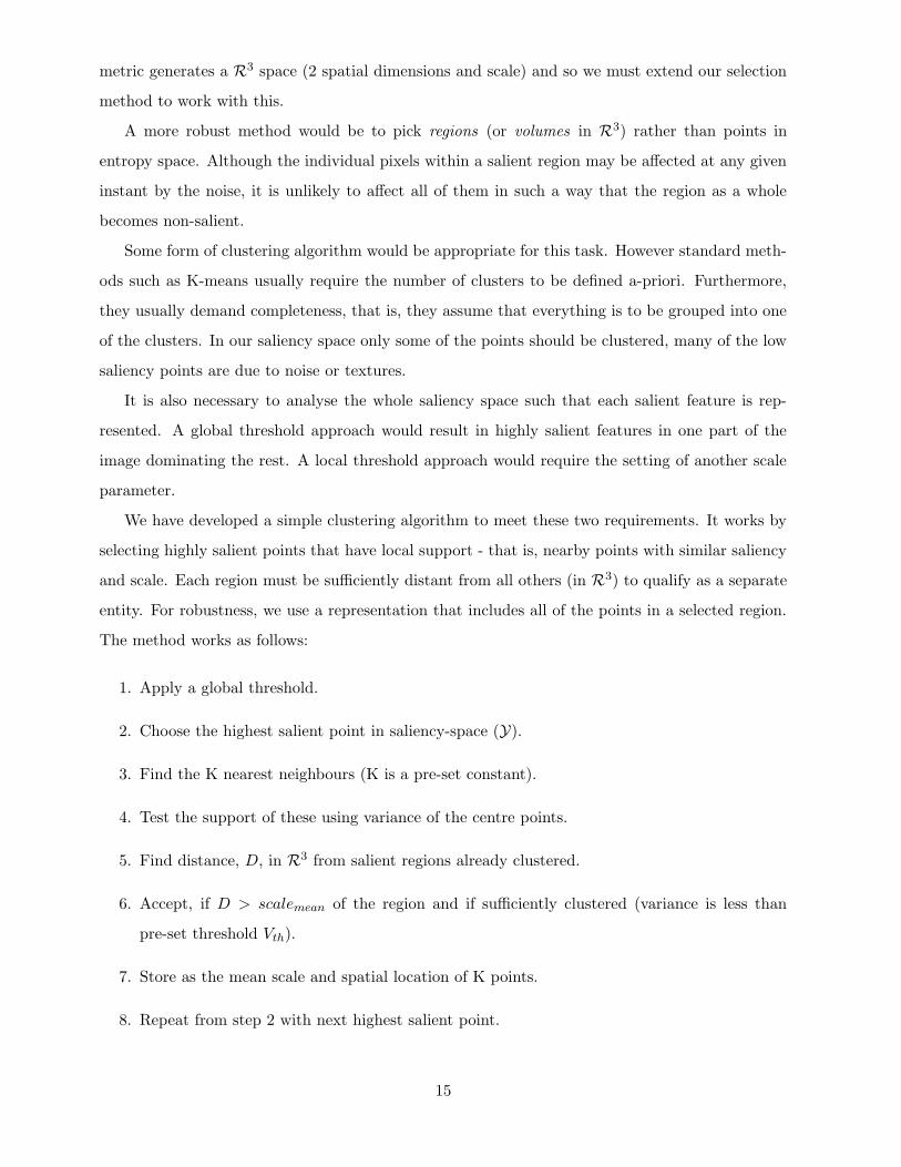
We have developed a simple clustering algorithm to meet these two requirements. It works by

selecting highly salient points that have local support - that is, nearby points with similar saliency

and scale. Each region must be sufficiently distant from all others (in R3) to qualify as a separate

entity. For robustness, we use a representation that includes all of the points in a selected region.

The method works as follows:

1. Apply a global threshold.

2. Choose the highest salient point in saliency-space (Y).

3. Find the K nearest neighbours (K is a pre-set constant).

4. Test the support of these using variance of the centre points.

5. Find distance, D, in R3 from salient regions already clustered.

6. Accept, if D > scalemean of the region and if sufficiently clustered (variance is less than

pre-set threshold Vth).

7. Store as the mean scale and spatial location of K points.

8. Repeat from step 2 with next highest salient point.

15

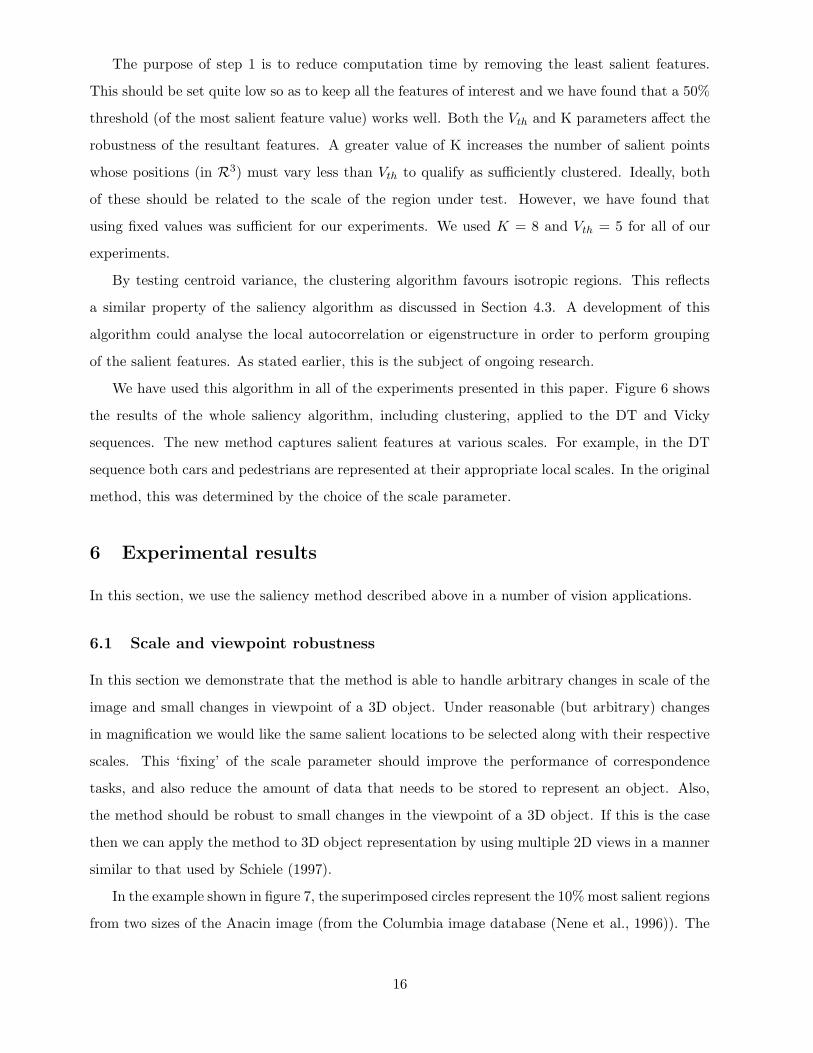
The purpose of step 1 is to reduce computation time by removing the least salient features.

This should be set quite low so as to keep all the features of interest and we have found that a 50%

threshold (of the most salient feature value) works well. Both the Vth and K parameters affect the

robustness of the resultant features. A greater value of K increases the number of salient points

whose positions (in R3) must vary less than Vth to qualify as sufficiently clustered. Ideally, both

of these should be related to the scale of the region under test. However, we have found that

using fixed values was sufficient for our experiments. We used K = 8 and Vth = 5 for all of our

experiments.

By testing centroid variance, the clustering algorithm favours isotropic regions. This reflects

a similar property of the saliency algorithm as discussed in Section 4.3. A development of this

algorithm could analyse the local autocorrelation or eigenstructure in order to perform grouping

of the salient features. As stated earlier, this is the subject of ongoing research.

We have used this algorithm in all of the experiments presented in this paper. Figure 6 shows

the results of the whole saliency algorithm, including clustering, applied to the DT and Vicky

sequences. The new method captures salient features at various scales. For example, in the DT

sequence both cars and pedestrians are represented at their appropriate local scales. In the original

method, this was determined by the choice of the scale parameter.

6 Experimental results

In this section, we use the saliency method described above in a number of vision applications.

6.1 Scale and viewpoint robustness

In this section we demonstrate that the method is able to handle arbitrary changes in scale of the

image and small changes in viewpoint of a 3D object. Under reasonable (but arbitrary) changes

in magnification we would like the same salient locations to be selected along with their respective

scales. This ‘fixing’ of the scale parameter should improve the performance of correspondence

tasks, and also reduce the amount of data that needs to be stored to represent an object. Also,

the method should be robust to small changes in the viewpoint of a 3D object. If this is the case

then we can apply the method to 3D object representation by using multiple 2D views in a manner

similar to that used by Schiele (1997).

In the example shown in figure 7, the superimposed circles represent the 10%most salient regions

from two sizes of the Anacin image (from the Columbia image database (Nene et al., 1996)). The

16

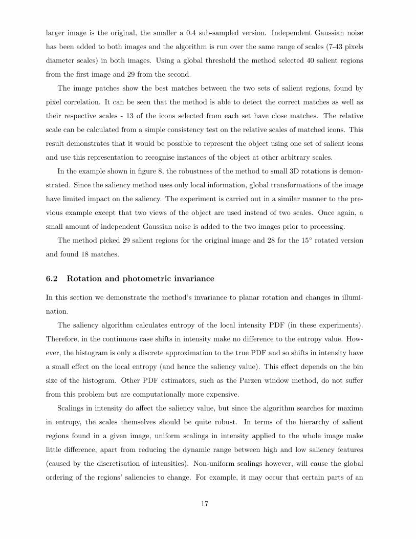
larger image is the original, the smaller a 0.4 sub-sampled version. Independent Gaussian noise

has been added to both images and the algorithm is run over the same range of scales (7-43 pixels

diameter scales) in both images. Using a global threshold the method selected 40 salient regions

from the first image and 29 from the second.

The image patches show the best matches between the two sets of salient regions, found by

pixel correlation. It can be seen that the method is able to detect the correct matches as well as

their respective scales - 13 of the icons selected from each set have close matches. The relative

scale can be calculated from a simple consistency test on the relative scales of matched icons. This

result demonstrates that it would be possible to represent the object using one set of salient icons

and use this representation to recognise instances of the object at other arbitrary scales.

In the example shown in figure 8, the robustness of the method to small 3D rotations is demon-

strated. Since the saliency method uses only local information, global transformations of the image

have limited impact on the saliency. The experiment is carried out in a similar manner to the pre-

vious example except that two views of the object are used instead of two scales. Once again, a

small amount of independent Gaussian noise is added to the two images prior to processing.

The method picked 29 salient regions for the original image and 28 for the 15◦ rotated version

and found 18 matches.

6.2 Rotation and photometric invariance

In this section we demonstrate the method’s invariance to planar rotation and changes in illumi-

nation.

The saliency algorithm calculates entropy of the local intensity PDF (in these experiments).

Therefore, in the continuous case shifts in intensity make no difference to the entropy value. How-

ever, the histogram is only a discrete approximation to the true PDF and so shifts in intensity have

a small effect on the local entropy (and hence the saliency value). This effect depends on the bin

size of the histogram. Other PDF estimators, such as the Parzen window method, do not suffer

from this problem but are computationally more expensive.

Scalings in intensity do affect the saliency value, but since the algorithm searches for maxima

in entropy, the scales themselves should be quite robust. In terms of the hierarchy of salient

regions found in a given image, uniform scalings in intensity applied to the whole image make

little difference, apart from reducing the dynamic range between high and low saliency features

(caused by the discretisation of intensities). Non-uniform scalings however, will cause the global

ordering of the regions’ saliencies to change. For example, it may occur that certain parts of an

17

image are illuminated better and hence higher variations in intensity are observed in that area. In

an extreme case, probably such areas would be more perceptually salient. However, the saliency

of a given region with respect to its local neighbourhood should be quite robust; that is, the local

ordering of saliencies should be robust. Therefore a local post-processing clustering technique, such

as described in Section 5, can overcome such problems.

In the case of rotation we expect the method to be invariant because the saliency algorithm

uses circular local windows to sample the image. Discretisation may cause some problems at the

smaller scales, however sub-pixel methods may be used to alleviate these.

Figure 9 shows the effect on the salient features of a 70% scaling (contrast reduction) of the

image intensity values and a 45◦ clockwise rotation. The lower diagrams show the so-called Sparse

Iconic representation used by Gilles. This shows the ‘icons’ matched by the algorithm in their

image positions and scales.

6.3 Object Tracking and Recognition

In this section, our aim is to motivate the use of our saliency method in recognition and tracking

tasks. In such tasks, two requirements of features and descriptions are that they should be robust,

and relevant. The former is necessary to ensure stable descriptions under variations in viewing

conditions; the latter, because it is desirable to relate descriptions to objects or parts thereof.

The purpose of this experiment is to demonstrate that features selected by our method are

persistent in several instances of an object in a scene. The application is a simplified recognition

and tracking scenario where the task is to identify close matches of a previously defined object

in an image sequence, treating each frame independently. The persistence of features builds on

the results of the previous sections and demonstrates robustness in a real scenario. By matching

features with a model, we test their relevance with respect to the image objects they represent.

There was no attempt to develop a Kalman or Condensation (Blake and Isard, 1997) tracker.

Such a tracker would further help the system in practice, but that is not the issue here. Treating

each image independently represents a worst-case scenario that obviously could be improved by

combining the ideas here with a tracker.

We used two sequences: the DT sequence from KOGS/IAKS Universitat Karlsruhe, and the

Vicky sequence. The models consisted of the clustered most salient regions and their scales found

by running our algorithm on the (sub-)images shown in the top-left of figures 10 and 11. These are

simply manually cropped from one frame in each sequence. In the Vicky experiment, two ‘takes’

of the sequence were available. We built the model from a single frame from one, and conducted

18

the experiment using the other.

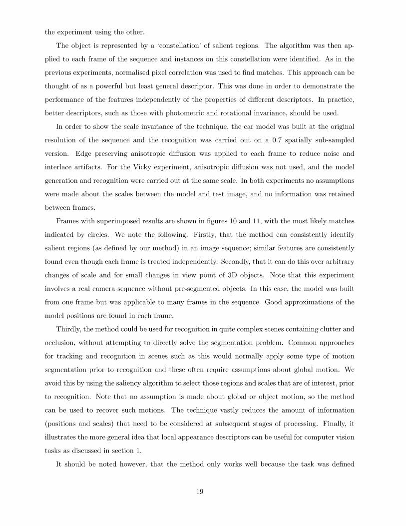
The object is represented by a ‘constellation’ of salient regions. The algorithm was then ap-

plied to each frame of the sequence and instances on this constellation were identified. As in the

previous experiments, normalised pixel correlation was used to find matches. This approach can be

thought of as a powerful but least general descriptor. This was done in order to demonstrate the

performance of the features independently of the properties of different descriptors. In practice,

better descriptors, such as those with photometric and rotational invariance, should be used.

In order to show the scale invariance of the technique, the car model was built at the original

resolution of the sequence and the recognition was carried out on a 0.7 spatially sub-sampled

version. Edge preserving anisotropic diffusion was applied to each frame to reduce noise and

interlace artifacts. For the Vicky experiment, anisotropic diffusion was not used, and the model

generation and recognition were carried out at the same scale. In both experiments no assumptions

were made about the scales between the model and test image, and no information was retained

between frames.

Frames with superimposed results are shown in figures 10 and 11, with the most likely matches

indicated by circles. We note the following. Firstly, that the method can consistently identify

salient regions (as defined by our method) in an image sequence; similar features are consistently

found even though each frame is treated independently. Secondly, that it can do this over arbitrary

changes of scale and for small changes in view point of 3D objects. Note that this experiment

involves a real camera sequence without pre-segmented objects. In this case, the model was built

from one frame but was applicable to many frames in the sequence. Good approximations of the

model positions are found in each frame.

Thirdly, the method could be used for recognition in quite complex scenes containing clutter and

occlusion, without attempting to directly solve the segmentation problem. Common approaches

for tracking and recognition in scenes such as this would normally apply some type of motion

segmentation prior to recognition and these often require assumptions about global motion. We

avoid this by using the saliency algorithm to select those regions and scales that are of interest, prior

to recognition. Note that no assumption is made about global or object motion, so the method

can be used to recover such motions. The technique vastly reduces the amount of information

(positions and scales) that need to be considered at subsequent stages of processing. Finally, it

illustrates the more general idea that local appearance descriptors can be useful for computer vision

tasks as discussed in section 1.

It should be noted however, that the method only works well because the task was defined

19

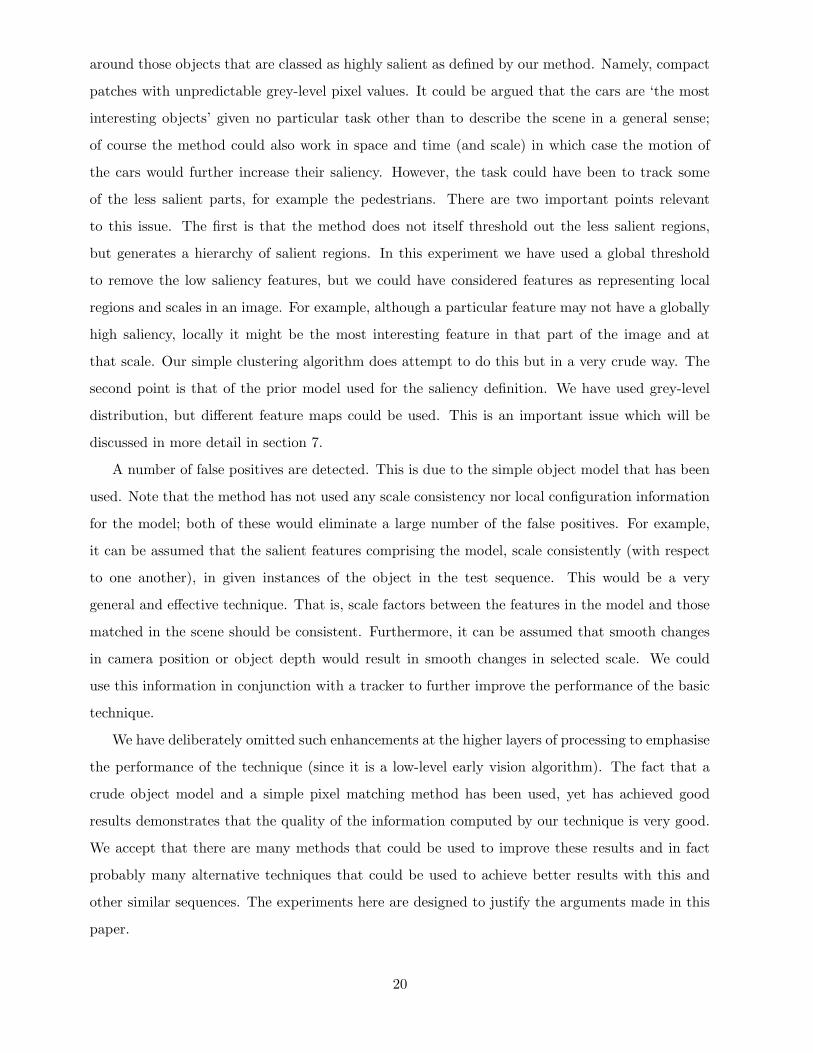
around those objects that are classed as highly salient as defined by our method. Namely, compact

patches with unpredictable grey-level pixel values. It could be argued that the cars are ‘the most

interesting objects’ given no particular task other than to describe the scene in a general sense;

of course the method could also work in space and time (and scale) in which case the motion of

the cars would further increase their saliency. However, the task could have been to track some

of the less salient parts, for example the pedestrians. There are two important points relevant

to this issue. The first is that the method does not itself threshold out the less salient regions,

but generates a hierarchy of salient regions. In this experiment we have used a global threshold

to remove the low saliency features, but we could have considered features as representing local

regions and scales in an image. For example, although a particular feature may not have a globally

high saliency, locally it might be the most interesting feature in that part of the image and at

that scale. Our simple clustering algorithm does attempt to do this but in a very crude way. The

second point is that of the prior model used for the saliency definition. We have used grey-level

distribution, but different feature maps could be used. This is an important issue which will be

discussed in more detail in section 7.

A number of false positives are detected. This is due to the simple object model that has been

used. Note that the method has not used any scale consistency nor local configuration information

for the model; both of these would eliminate a large number of the false positives. For example,

it can be assumed that the salient features comprising the model, scale consistently (with respect

to one another), in given instances of the object in the test sequence. This would be a very

general and effective technique. That is, scale factors between the features in the model and those

matched in the scene should be consistent. Furthermore, it can be assumed that smooth changes

in camera position or object depth would result in smooth changes in selected scale. We could

use this information in conjunction with a tracker to further improve the performance of the basic

technique.

We have deliberately omitted such enhancements at the higher layers of processing to emphasise

the performance of the technique (since it is a low-level early vision algorithm). The fact that a

crude object model and a simple pixel matching method has been used, yet has achieved good

results demonstrates that the quality of the information computed by our technique is very good.

We accept that there are many methods that could be used to improve these results and in fact

probably many alternative techniques that could be used to achieve better results with this and

other similar sequences. The experiments here are designed to justify the arguments made in this

paper.

20

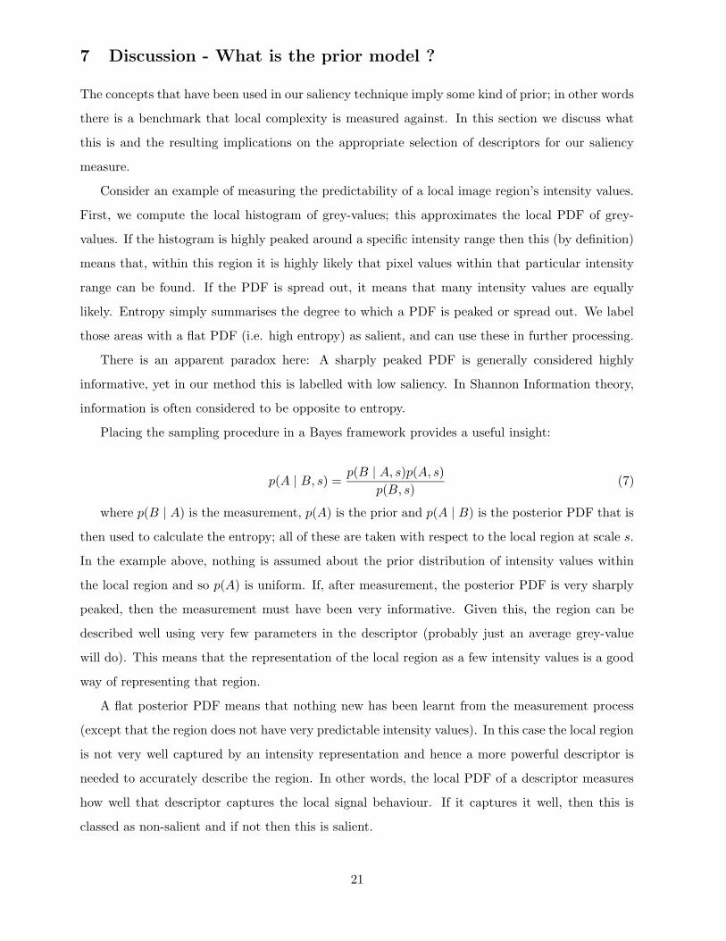
7 Discussion - What is the prior model ?

The concepts that have been used in our saliency technique imply some kind of prior; in other words

there is a benchmark that local complexity is measured against. In this section we discuss what

this is and the resulting implications on the appropriate selection of descriptors for our saliency

measure.

Consider an example of measuring the predictability of a local image region’s intensity values.

First, we compute the local histogram of grey-values; this approximates the local PDF of grey-

values. If the histogram is highly peaked around a specific intensity range then this (by definition)

means that, within this region it is highly likely that pixel values within that particular intensity

range can be found. If the PDF is spread out, it means that many intensity values are equally

likely. Entropy simply summarises the degree to which a PDF is peaked or spread out. We label

those areas with a flat PDF (i.e. high entropy) as salient, and can use these in further processing.

There is an apparent paradox here: A sharply peaked PDF is generally considered highly

informative, yet in our method this is labelled with low saliency. In Shannon Information theory,

information is often considered to be opposite to entropy.

Placing the sampling procedure in a Bayes framework provides a useful insight:

p(A | B, s) =p(B | A, s)p(A, s)

p(B, s)(7)

where p(B | A) is the measurement, p(A) is the prior and p(A | B) is the posterior PDF that is

then used to calculate the entropy; all of these are taken with respect to the local region at scale s.

In the example above, nothing is assumed about the prior distribution of intensity values within

the local region and so p(A) is uniform. If, after measurement, the posterior PDF is very sharply

peaked, then the measurement must have been very informative. Given this, the region can be

described well using very few parameters in the descriptor (probably just an average grey-value

will do). This means that the representation of the local region as a few intensity values is a good

way of representing that region.

A flat posterior PDF means that nothing new has been learnt from the measurement process

(except that the region does not have very predictable intensity values). In this case the local region

is not very well captured by an intensity representation and hence a more powerful descriptor is

needed to accurately describe the region. In other words, the local PDF of a descriptor measures

how well that descriptor captures the local signal behaviour. If it captures it well, then this is

classed as non-salient and if not then this is salient.

21

It follows that the technique can be considered to model the non-salient parts of a signal rather

than the salient parts. Saliency is defined as those parts of the signal that cannot be represented

well by our prior model. Therefore the entropy of a descriptor tells us how well that descriptor

captures the local region’s data. This is opposite to the way in which most feature extraction and

visual saliency techniques work, but is actually rather intuitive. Those parts of an image that are

most informative are those that do not get modeled well (or predicted) by our prior assumptions or

put another way: if we can model them then they’re probably not all that interesting. We assume

that the prior model captures the common or widespread behaviour of the signal. In the examples

used in this paper the non-saliency model is a piecewise flat local image patch and the assumption

here is that piecewise flat parts are very common and not very interesting.

7.1 Choosing Descriptors for Saliency

In this paper all the results and examples that have been presented have used the local intensity

as the descriptor for saliency. Given the above re-interpretation, the technique can be stated as

: Given a descriptor with one (or more) free parameters, describe the local region’s signal; its

saliency is inversely related to how good (or compact) this description is. Therefore in designing

appropriate descriptors for saliency all the parameters of what is non-salient should be included in

the descriptor. For example, for selection of salient regions in fingerprint images, an edge detector

at multiple orientations and scales can be used. The descriptor, in this case, is a region containing

a line with a variable scale and orientation. This would model low saliency as a single line at some

orientation at a single thickness. In this case salient regions could be where there are multiple lines

joining together, as occurs at bifurcations. Figure 12 shows an example of this. We have used a

Gaussian derivative at a particular scale and assigned a single dominant orientation to each pixel

location. Our multiscale saliency algorithm has then been applied to this feature map and the

most salient parts shown with superimposed circles.

7.2 Saliency and description

In the Introduction, it was argued that the use of saliency methods should enable better and more

compact image descriptions to be obtained. This should improve the performance of correspondence

and matching tasks. In this section we discuss the link between saliency and description tasks within

our framework.

Approaches in the literature have tended to select salient features separately from their subse-

quent description. Gilles (Gilles, 1998) does not suggest any link between the two processes and

22

uses the image patches directly. Schmid and Mohr (1997) use the Local Jet at multiple scales to

describe the image near Interest points. However there is no justification of why these descriptors

are good for the particular choice of salient feature.

Earlier it was discussed that our saliency method could be considered to model the low-saliency

parts of the image. Entropy of a local descriptor measures the degree to which that descriptor

captures local signal behaviour and these are chosen to represent efficiently (from an information

theory point of view) those parts of an image which are non-salient. The regions which are classed

as highly salient are those which are not well represented by that descriptor and need different (more

powerful) descriptors. The entropy method can be used to test how well a descriptor performs.

We may generalise the approach. Rather than applying one saliency measure and then describing

the salient parts, we propose that a hierarchy of increasingly powerful descriptors be applied and

tested. At each level, we can extract the non-salient features which can be described well by the

descriptors at that level. The salient parts can then be tested using more powerful descriptors until

all the image has been sufficiently described.

In Gilles’ original work, salient local image patches were described as vectors of pixel values

for the subsequent matching task. This can be thought of as a very powerful descriptor (high

dimensional). We have used the same approach in our experiments. Different descriptors may be

used, which may have advantages such as photometric or rotational invariance.

7.3 Spectral and Wavelet entropy

In this section we discuss the relationship of our method to two related signal complexity measures,

Spectral entropy (Zheng et al., 1996) and Wavelet entropy (Starck and Murtagh, 1999). A corollary

of this relationship is that there are also strong links to image compression and Wavelet packet

best basis selection techniques (Coifman and Wickerhauser, 1992).

Spectral entropy is used by the Neural Network community to measure pattern complexity. It

is calculated directly from the Fourier coefficients of transformed signal. Wavelet entropy has been

proposed by Murtagh as a technique for image feature extraction and content description (Starck

and Murtagh, 1999). It also calculates entropy directly from the (Wavelet) basis coefficients, but

introduces a noise model which improves robustness. They are both multiscale in the sense that

they consider different scales in calculation of the complexity of the signal.

Both these methods can be considered in the context of our saliency technique as different local

descriptors of non-saliency. For example, in the case of Spectral entropy, if we were to classify as

salient those regions with many coefficients with similar magnitudes, then the prior model we have

23

used for non-saliency is that of a region containing a single frequency (band). The descriptors for

non-saliency form a much richer set in this case than in the intensity distribution case. Wavelet

entropy can be analysed in a similar manner. Furthermore, there may be benefits of using Spectral

or Wavelet entropy over intensity distribution entropy; one example is the noise model included in

the method used in (Starck and Murtagh, 1999).

Compression techniques commonly take advantage of the decorrelation properties of transforms

such as the Discrete Cosine Transform or the Wavelet Transform, to achieve compression. The idea

is that the signal is transformed into a set of decorrelated or orthogonal basis vectors which, after

appropriate quantisation, can represent the signal in a more efficient manner. The method works

most efficiently if the signals found in the source can be represented well by a small number of the

basis vectors - that is the basis set can synthesize the source signals with only a few parameters.

Our saliency method with a local descriptor set made from the local Fourier or Wavelet coefficients,

bears a strong resemblance to signal compression techniques. Non-salient parts of the image are

those that contain significant redundancy and can be compressed quite easily.

Entropy is also widely used in the selection of best basis in Wavelet packet methods (Coifman

and Wickerhauser, 1992). Here the basis with the minimum local entropy is classified as the best;

that is, the one with the fewest negligible coefficients. Once again, there is a strong link with our

approach to saliency and description.

7.4 Saliency and segmentation

The task in segmentation is to group image pixels such that the groups satisfy some definition of

homogeneity. For example this may be that the regions are piecewise continuous in intensity, of

similar texture, or have similar motion vectors. In the entropy of intensity approach to saliency, the

task is to find groups of pixels which are different from each other (but close spatially) according

to the assumed definition of non-saliency. In the intensity distribution local descriptor that has

been used for the majority of the experiments in this paper, groups containing many different pixel

values in equal proportion are considered salient. In this way, the method can be viewed as the

opposite to the classic segmentation problem. The salient regions can be considered as the outliers

of the homogeneous regions after segmentation. In fact Gilles did suggest that his method could

be used to select seed points for a segmentation algorithm.

24

8 Conclusion

In this paper we have presented a discussion of three separate but closely related issues common

in many computer vision problems: saliency, scale, and image description.

In many computer vision tasks we would like to extract ‘meaningful’ and general descriptors

of image content. Descriptors have to be appropriate to the task at hand to be useful, but early

vision in humans is believed to operate with little contextual information. From the popular pre-

attentive and attentive models of early vision, and from several recent results it is known that local

features can be ‘good enough’ to solve many computer vision tasks. We have discussed the idea of

visual saliency which suggests that certain regions of the image are better than others at describing

content and we have suggested that this approach can solve some of the problems associated with

purely local methods.

Motivated by the promising results obtained by Gilles, we have investigated his local complexity

approach to visual saliency applied to a wide range of image source material including image

sequences. Our experiments showed that local scale selection was necessary but furthermore that

the method had to be extended to consider saliency across scale as well as spatial dimensions.

We have introduced a novel saliency method that builds on Gilles ideas but automatically selects

appropriate scales for analysis and can compare the scale-space behaviour of image features. We

then presented results showing the performance of the technique, in particular its invariance to

scale changes in the image and view point changes in 3D objects. We then applied the technique

to an object recognition and tracking task in an image sequence. Using a crude object model and

pixel correlation matching, the technique was successful in identifying matches of the model in an

image sequence consisting of a complex scene. In these examples, we used a minimal set of prior

assumptions in order to highlight the performance of the basic technique. Further enhancements

can be made to the technique by using, for example, a Condensation or Kalman tracker or by

making basic assumptions about the consistency of scales between model and image, or smoothness

of changes in position and scale between frames in an image sequence. The use of such assumptions

is the subject of further investigation and results will be reported in a future paper. We are also

investigating the application of the technique to large database object recognition problems and

will report on these results in a future paper.

In the last section we investigated the links between saliency and image description. In many

approaches to saliency these two issues have been separately handled. Features that have been

selected using a saliency algorithm are then described by using an arbitrary description method

(and in some cases arbitrary scales). On the contrary we argue that the two tasks should be

25

considered as parts of the same problem. Having analysed the prior model for saliency that we have

used in the experiments, we conclude that the method measures how well a given local descriptor

captures local signal behaviour. Low saliency regions are those that can be modeled very well by

the chosen local descriptor (in information theory this means ‘in few bits’; in signal processing this

can mean ‘good signal to noise ratio’). In the example of local intensity distribution low saliency

regions are those that are piecewise flat. In other words the prior model should be designed such

that the non-salient features are well described; the saliency descriptor models the background

rather than foreground. This approach is quite distinct from conventional approaches to saliency.

We presented an example where we wish to find the salient parts in a fingerprint image. The model

of non-saliency in this case is a single direction edge at a particular scale. Salient parts are those

with many directions and scales. The method can in this way be generalised for any prior model.

Subsequent description of that image feature should be done by a more discriminating descriptor

than the one used for saliency.

Having made this observation, a number of other relations become obvious: Spectral/Wavelet

entropy are simply the same method but with different local descriptors; Segmentation is the

opposite to saliency (as we have defined it); strong connections exist to compression coding where

redundancy (low-saliency) is taken advantage of to achieve compression.

Acknowledgments

This research was sponsored by a Motorola University Partners in Research grant. We would like

to thank Paola Hobson and Ken Crisler for the many very useful discussions we have had during

the course of this work.

26

References

L. Alvarez, P. Lions, and J. Morel. Image selective smoothing and edge detection by nonlinear

diffusion. II. SIAM Journal on Numerical Analysis, 29(3):845–866, June 1992.

F. Bergholm. Edge focusing. In Proc. Int. Conf. on Pattern Recognition, pages 597–600, October

1986. Paris, France.

A. Blake and M. Isard. The CONDENSATION algorithm — conditional density propagation and

applications to visual tracking. In Michael C. Mozer, Michael I. Jordan, and Thomas Petsche,

editors, Advances in Neural Information Processing Systems, volume 9, page 361. MIT Press:

Cambridge, MA., 1997.

P.J. Burt and E.H. Adelson. The Laplacian pyramid as a compact image code. IEEE Trans.

Communication, 31(4):532–540, April 1983.

O. Chomat, V.C. deVerdiere, D. Hall, and J.L. Crowley. Local scale selection for gaussian based

description techniques. In Proc. European Conf. Computer Vision, pages 117–133, 2000.

R. Coifman and M. Wickerhauser. Entropy-based algorithms for best basis selection. IEEE Trans.

on Information Theory, 38(2):713–718, 1992.

R. Deriche and T. Giraudon. A computational approach for corner and vertex detection. Interna-

tional Journal of Computer Vision., 10(2):101–124, 1993.

Y. Dufournaud, C. Schmid, and R. Horaud. Matching images with different resolutions. In Proc.

Int. Conf. on Computer Vision and Pattern Recognition, pages I:612–618, 2000.

S. Gilles. Robust Description and Matching of Images. PhD thesis, University of Oxford, 1998.

C. Harris and M. Stephens. A combined corner and edge detector. In Proc. 4th Alvey Vision Conf,

pages 189–192, August 1988. Manchester.

M. Jagersand. Saliency maps and attention selection in scale and spatial coordinates: An infor-

mation theoretic approach. In Proc. Int. Conf. on Computer Vision, pages 195–202, 1995. MIT

Cambridge, MA.

B. Julesz. Dialogues on Perception. MIT Press, 1995.

J.J. Kœnderink. The structure of images. Biological Cybernetics, 50:363–370, 1984.

27

J.J. Kœnderink and A.J. van Doorn. Representation of local geometry in the visual system.

Biological Cybernetics, 63:291–297, 1987.

Y.G. Leclerc. Constructing simple stable descriptions for image partitioning. Int. Journal of

Computer Vision., 3:73–102, 1989.

T. Lindeberg. On scale selection for differential operators. In Proc. 8th Scandinavian Conf. on

Image Analysis, pages 857–866, Tromso, Norway, May 1993.

T. Lindeberg. Junction detection with automatic selection of detection scales and localization

scales. In Proc. Int. Conf. on Image Processing, pages 924–928, November 1994.

T. Lindeberg and B.M. ter Haar Romeny. Linear Scale-Space: I. Basic Theory, II. Early Visual

Operations. In Geometry-Driven Diffusion, B.M. ter Haar Romeny (Ed.). Kluwer Academic

Publishers, Dordrecht, The Netherlands., 1994.

S. Mallat. A Wavelet Tour of Signal Processing. Academic Press, San Diego, 1998.

D. Marr. Vision: a Computational Investigation into the Human Representation ond Processing of

Visual Information. W. H. Freeman, San Francisco, 1982.

D. Marr and E. Hildreth. Theory of edge detection. Proceedings Royal Society of London Bulletin,

204:301–328, 1979.

R. Milanese. Detecting Salient Regions in an Image: From Biological Evidence to Computer Im-

plementation. PhD thesis, University of Geneva, 1993.

F. Mokhtarian and R. Suomela. Robust image corner detection through curvature scale space.

IEEE Trans. Pattern Analysis and Machine Intelligence, 20(12), 1998.

U. Neisser. Visual search. Scientific American, 210(6):94–102, June 1964.

S. Nene, S. Nayar, and H. Murase. Columbia image object library. Technical report, Department

of Computer Science, Columbia University, 1996.

P. Perona and J. Malik. Scale space and edge detection using anisotropic diffusion. In Proc. Int.

Conf. on Computer Vision and Pattern Recognition, pages 16–22, 1988.

B. Schiele. Object Recognition Using Multidimensional Receptive Field Histograms. PhD thesis,

I.N.P. de Grenoble, 1997.

28

C. Schmid and R. Mohr. Local greyvalue invariants for image retrieval. IEEE Trans. Pattern

Analysis and Machine Intelligence, 19(5):530–535, 1997.

C. Schmid, R. Mohr, and C. Bauckhage. Comparing and evaluating interest points. In Proc. Int.

Conf. on Computer Vision, pages 230–235, 1998.

A. Sha’ashua and S. Ullman. Structural saliency: the detection of globally salient structures using

a locally connected network. In Proc. Int. Conf. on Computer Vision, pages 321–327, 1988.

Tampa, Fl.

J. Starck and F. Murtagh. Multiscale entropy filtering. EURASIP Signal Processing, pages 147–165,

1999.

M.J. Swain and D.H. Ballard. Colour indexing. International Journal of Computer Vision, 7(1):

11–32, 1995.

B.M. ter Haar Romeny. Introduction to Scale-Space Theory: Multiscale Geometric Image Analysis.

PhD thesis, Utrecht University, 1996.

A. Treisman. Preattentive processing in vision. Computer Vision, Graphics, and Image Processing,

31(2):156–177, 1985.

K.N. Walker, T.F. Cootes, and C.J. Taylor. Locating salient facial features using image invariants.

In Int. Conf. on Automatic Face and Gesture Recognition, 1998a. Nara, Japan.

K.N. Walker, T.F. Cootes, and C.J. Taylor. Locating salient object features. In Proc. British

Machine Vision Conference, pages 557–566, 1998b. Southampton, UK.

J. Weickert. A review of nonlinear diffusion filtering. Lecture Notes in Computer Science, 1252:

3–28, 1997.

A. Winter, H. Maitre, N. Cambou, and E. Legrand. Entropy and multiscale analysis : an original

feature extraction algorithm for aerial and satellite images. In Proc. Int. Conf. on Acoustics,

Speech, and Signal Processing. IEEE, April 1997.

A. Witkin. Scale-space filtering. In Proc. Int. Joint Conf. on Artificial Intelligence. Karlsruhe,

Germany, 1983.

B.Y. Zheng, W. Qian, and L.P. Clarke. Digital mammography - mixed feature neural network with

spectral entropy decision for detection of microcalcifications. IEEE Trans. on Medical Imaging,

15(5):589–597, 1996.

29

S.C. Zhu and A. Yuille. Region competition: Unifying snakes, region growing, and bayes/mdl for

multiband image segmentation. IEEE Pattern Analysis and Machine Intelligence, 18(9):884–900,

September 1996.

30

Figure 1: Examples of Visual Saliency.

31

Figure 2: The local histograms of intensity. Uniform images tend to have peaked histograms

indicating a low complexity (or high predictability). Neighbourhoods with structures have flatter

distributions, that is, a higher complexity. Reproduced with permission from (Gilles, 1998).

32

Figure 3: Example frames from the application of the original Gilles algorithm to the DT (top)

and Vicky (bottom) sequences.

33

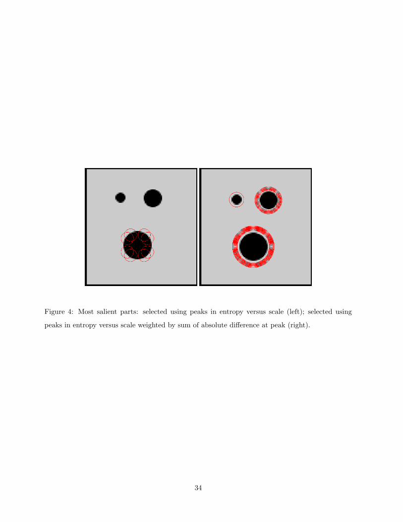
Figure 4: Most salient parts: selected using peaks in entropy versus scale (left); selected using

peaks in entropy versus scale weighted by sum of absolute difference at peak (right).

34

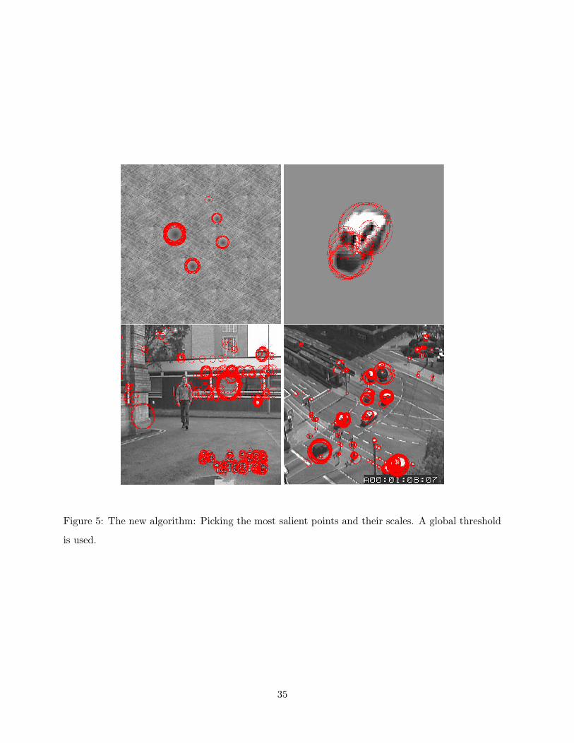
Figure 5: The new algorithm: Picking the most salient points and their scales. A global threshold

is used.

35

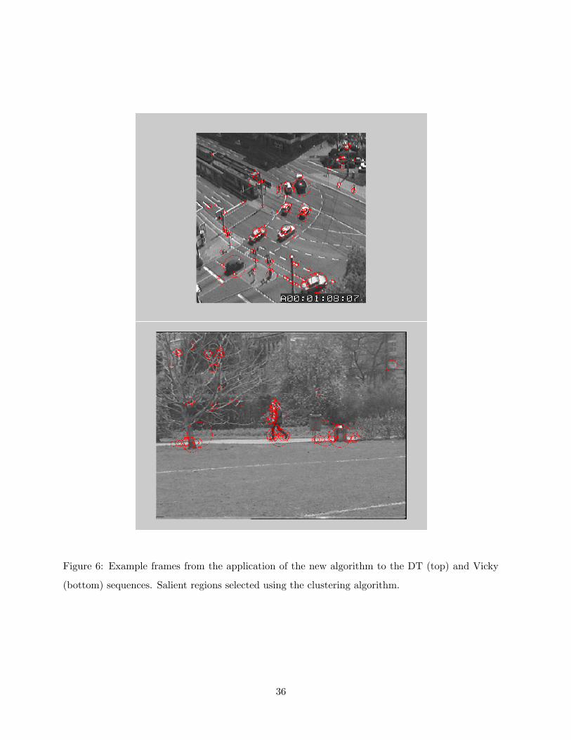
Figure 6: Example frames from the application of the new algorithm to the DT (top) and Vicky

(bottom) sequences. Salient regions selected using the clustering algorithm.

36

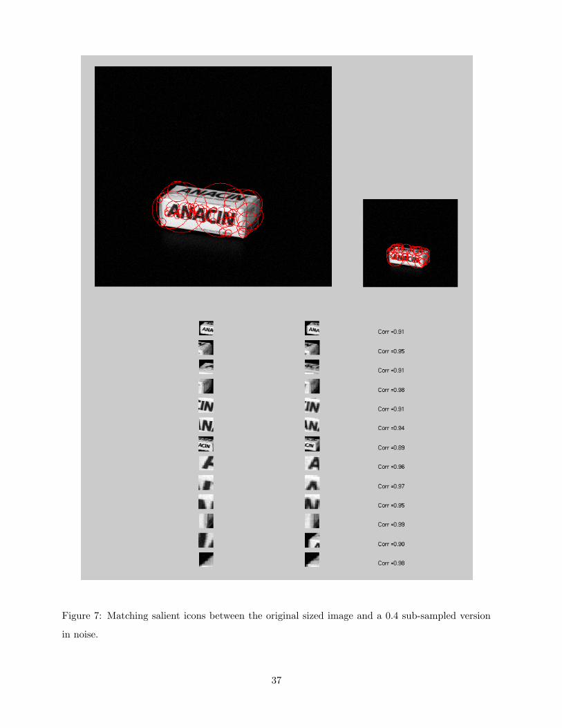
Figure 7: Matching salient icons between the original sized image and a 0.4 sub-sampled version

in noise.

37

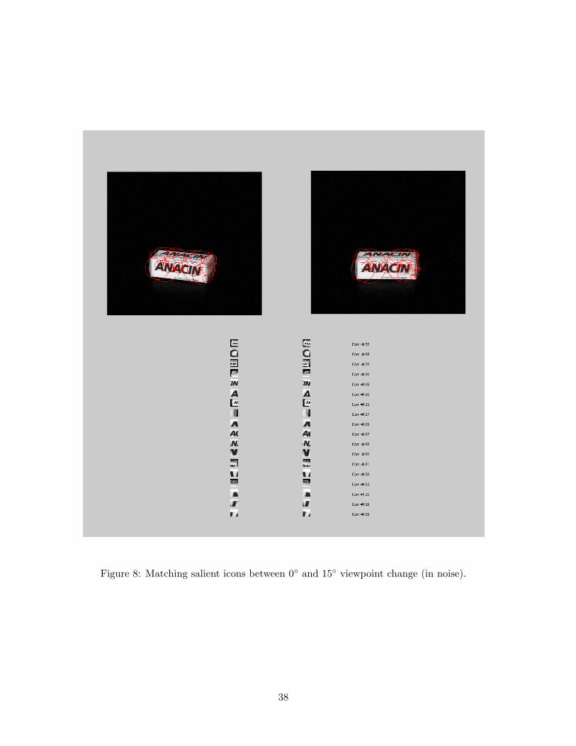
Figure 8: Matching salient icons between 0◦ and 15◦ viewpoint change (in noise).

38

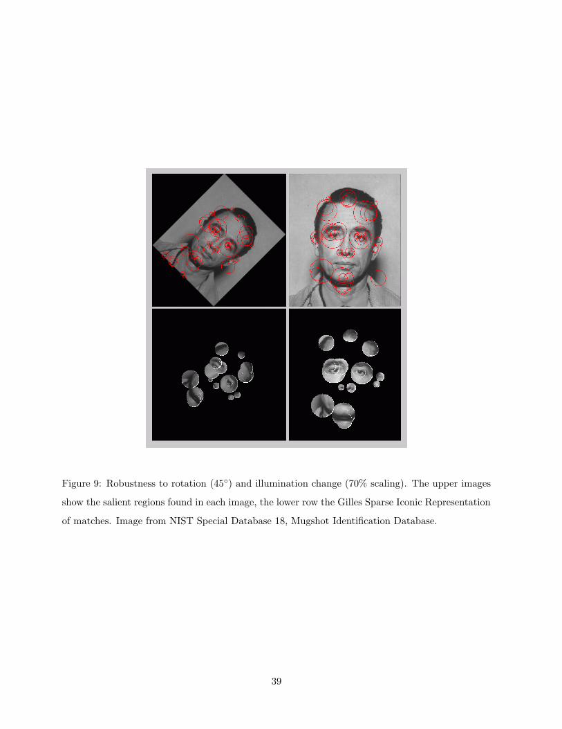
Figure 9: Robustness to rotation (45◦) and illumination change (70% scaling). The upper images

show the salient regions found in each image, the lower row the Gilles Sparse Iconic Representation

of matches. Image from NIST Special Database 18, Mugshot Identification Database.

39

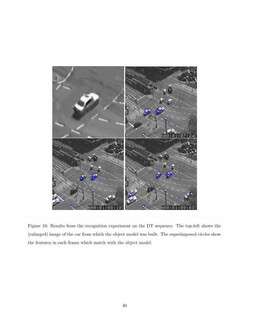
Figure 10: Results from the recognition experiment on the DT sequence. The top-left shows the

(enlarged) image of the car from which the object model was built. The superimposed circles show

the features in each frame which match with the object model.

40

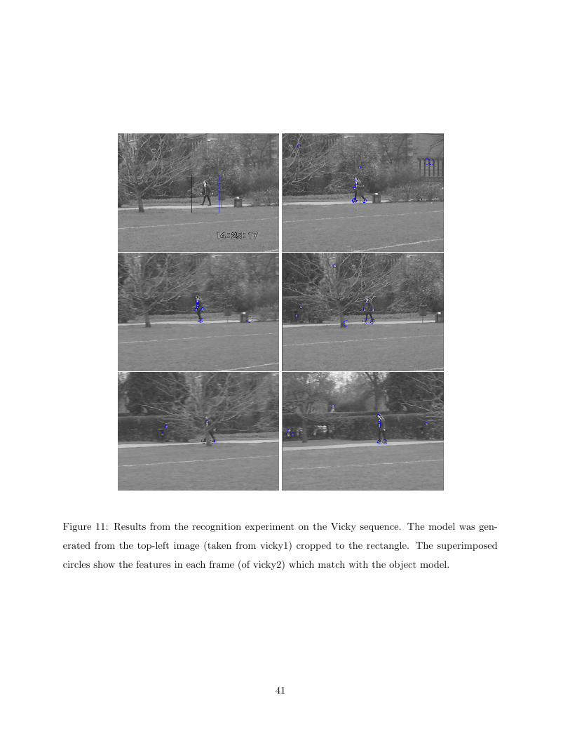
Figure 11: Results from the recognition experiment on the Vicky sequence. The model was gen-

erated from the top-left image (taken from vicky1) cropped to the rectangle. The superimposed

circles show the features in each frame (of vicky2) which match with the object model.

41

Figure 12: Using dominant edge directions at a certain scale as the non-salient descriptor on a

fingerprint image.

42

List of Figures

1 Examples of Visual Saliency. . . . . . . . . . . . . . . . . . . . . . . . . . . . . . . . 31

2 The local histograms of intensity. Uniform images tend to have peaked histograms

indicating a low complexity (or high predictability). Neighbourhoods with structures

have flatter distributions, that is, a higher complexity. Reproduced with permission

from (Gilles, 1998). . . . . . . . . . . . . . . . . . . . . . . . . . . . . . . . . . . . . . 32

3 Example frames from the application of the original Gilles algorithm to the DT (top)

and Vicky (bottom) sequences. . . . . . . . . . . . . . . . . . . . . . . . . . . . . . . 33

4 Most salient parts: selected using peaks in entropy versus scale (left); selected using

peaks in entropy versus scale weighted by sum of absolute difference at peak (right). 34

5 The new algorithm: Picking the most salient points and their scales. A global

threshold is used. . . . . . . . . . . . . . . . . . . . . . . . . . . . . . . . . . . . . . . 35

6 Example frames from the application of the new algorithm to the DT (top) and

Vicky (bottom) sequences. Salient regions selected using the clustering algorithm. . 36

7 Matching salient icons between the original sized image and a 0.4 sub-sampled ver-

sion in noise. . . . . . . . . . . . . . . . . . . . . . . . . . . . . . . . . . . . . . . . . 37

8 Matching salient icons between 0◦ and 15◦ viewpoint change (in noise). . . . . . . . 38

9 Robustness to rotation (45◦) and illumination change (70% scaling). The upper

images show the salient regions found in each image, the lower row the Gilles Sparse

Iconic Representation of matches. Image from NIST Special Database 18, Mugshot

Identification Database. . . . . . . . . . . . . . . . . . . . . . . . . . . . . . . . . . . 39

10 Results from the recognition experiment on the DT sequence. The top-left shows

the (enlarged) image of the car from which the object model was built. The su-

perimposed circles show the features in each frame which match with the object

model. . . . . . . . . . . . . . . . . . . . . . . . . . . . . . . . . . . . . . . . . . . . . 40

11 Results from the recognition experiment on the Vicky sequence. The model was

generated from the top-left image (taken from vicky1) cropped to the rectangle.

The superimposed circles show the features in each frame (of vicky2) which match

with the object model. . . . . . . . . . . . . . . . . . . . . . . . . . . . . . . . . . . . 41

12 Using dominant edge directions at a certain scale as the non-salient descriptor on a

fingerprint image. . . . . . . . . . . . . . . . . . . . . . . . . . . . . . . . . . . . . . . 42

43

Footnotes

Affiliation of Authors - Robotics Research Laboratory, Department of Engineering Science, Uni-

versity of Oxford, Parks Road, Oxford OX1 3PJ, U.K.

(*) Timor Kadir is the recipient of a Motorola University Partners in Research grant.

(1) We do not advocate the use of one particular scale space representation in our work. Rather we

are interested in scale selection and the extension of saliency to operate over scale. We have used

a circular top-hat sampling kernel to generate our scale space for reasons of simplicity, rotational

invariance (in the image plane) and because it does not alter the statistical properties of the local

descriptor.

(2) Copyright (c) 1998 by H.H. Nagel. Institut fur Algorithmen und Kognitive Systeme. Fakultat

fur Informatik. Universitat Karlsruhe (TH). Postfach 6980.D - 76128 Karlsruhe, Germany.

(3) Histograms are not confined to intensity; they may be any local attribute such as colour or

edge strength, direction or phase.

(4) Note, these operators do not exclusively select features that are perceived to be the corners of

objects; rather, they compute sets of zero measure typified by their peaked autocorrelation.

(5) Gilles was primarily interested in the matching of aerial images.

44

Address for correspondence

Timor Kadir.

Wolfson College,

Oxford.

Oxfordshire.

OX2 6UD.

U.K.

45