saha institute of nuclear physics, kolkata
TRANSCRIPT

1
Atomic Force Microscopy beyond topography and electrochemical analysis: Graphene, Zinc
Oxide and Bacteria
By
Anuradha Bhattacharya
PHYS05200804005
Saha Institute Of Nuclear Physics, Kolkata
A thesis submitted to the
Board of Studies in Physical Sciences
In partial fulfillment of requirements for the Degree of
DOCTOR OF PHILOSOPHY of
HOMI BHABHA NATIONAL INSTITUTE
January, 2015
2
List of Publications arising from the thesis
Journal
1) A. Bhattacharya, V.P. Rao, C. Jain, A. Ghose, S. Banerjee, Bio-sensing property of gold
coated ZnO nanorods. Materials Letters, 2014,117(3), pp 128–130
A. Bhattacharya, S. Banerjee, Identifying bacterial fragments on morphologically
similar substrate using UAFM. Micron 2014, 60(4), pp 1–4
S. Panigrahi*, A. Bhattacharya*, D. Bandyopadhyay, S. J. Grabowski, D. Bhattacharyya
and S. Banerjee (2011), Wetting Property of the Edges of Monoatomic Step on Graphite:
Frictional-Force Microscopy and ab Initio Quantum Chemical Studies. J. Phys. Chem. C, 115,
14819-14826, (*SP and AB both are first authors with equal contribution with SP doing the
theoretical part and AB doing the experimental part)
4) S. Panigrahi*, A. Bhattacharya*, S. Banerjee, D. Bhattacharyya, Interaction of
Nucleobases with Wrinkled Graphene Surface: Dispersion Corrected DFT and AFM Studies. J.
Phys. Chem. C, 2012, 116(7), pp 4374–4379, (*SP and AB both are first authors with equal
contribution with SP doing the theoretical part and AB doing the experimental part)
Conferences
Anuradha Bhattacharya, Chhavi Jain, V. Padmanapan Rao and S. Banerjee, Gold coated
ZnO nanorod biosensor for glucose detection. AIP Conf. Proc. 1447, 295 (2012)
S. Banerjee, D. Bhattacharya, S. Panigrahi, A. Bhattacharya, M. Sardar, N. Gayathri, A. K.
Tyagi and Baldev Raj, Electronic, wetting, stability and magnetic properties of graphene. AIP
Conf. Proc. 1447, 61 (2012)
J. Kaur, A. Rai Chowdhury, A. Bhattacharya, B. Ghosh, M. Sardar and S. Banerjee,
Emergence of long range magnetic interaction upon reduction of graphene oxide. AIP
Conf. Proc. 1447, 1233 (2012)

3
2
ACKNOWLEDGEMENTS:
I want to thank my guide Dr. Sangam Banerjee for his huge support. I would not
be able to do this if it wasn’t for him. I would also like to thank my laboratory
members for their support and encouragement. I would also like to thank my
institute Saha Institute Of Nuclear Physics, Kolkata for providing me with all the
facilities to conduct research.

4
CONTENTS
Synopsis 9
1. Chapter 1: Introduction 13
1.1 Structural conformations of graphene: Mother of all carbon forms 15
1.1.2 Electronic properties of graphene 18
1.2 Synthesis of graphene 20
1.2.1 Exfoliation using scotch tape 20
1.2.2 Unzipping of CNTs 22
1.2.3 Chemical Exfoliation 22
1.2.4 Supercritical CO2 method 23
1.2.5 Annealing graphite in oxygen rich atmosphere 23
1.2.6 Solvothermal Route 23
1.2.7 Chemical Route 24
1.2.8 Chemical Vapour Deposition 25
1.2.9 Sublimation (SiC) 25
1.3 Wetting property of graphene in relation to its electronic property 26
1.4 Wrinkles in graphene sheet 27
1.5 Magnetic and bio-sensing properties of graphene 28
1.6 Biosensors 29
1.7 Conclusion 31

5
2. Chapter 2: Experimental Methods
2.1 Introduction 38
2.1.1 Sample preparation 38
2.2 Experimental techniques 42
2.21 Contact mode of operation 43
2.2.2 Tapping Mode 45
2.2.3 Frictional Force Microscopy 45
2.2.4 Ultrasonic Force Microscopy (UFM) /
Atomic Force Acoustic Microscopy (AFAM) 50
2.2.5 Conducting tip AFM 51
2.3.1 Electrochemistry 52
2.3.2 Potentiostat 53
2.3.3 Galvanostat 53
2.3.4 Reference Electrode 53
2.3.4.1 Ag/AgCl reference elecrode 54
2.3.4.2 Calomel reference electrode 55
2.3.5 Counter Electrode 55
2.3.5.1 Platinum counter Electrode 55
2.3.6 Working Electrode 56
2.3.7 Faraday’s Law 56
2.3.9 Electrochemical Workstation 57

6
2.3.9.1 Cyclic Voltammogram 57
2.3.9.2 Amperometric Response 58
2.3.9.3 Electrochemical Impedance Spectoscopy 58
2.4 Basic principle of RAMAN spectroscopy 59
2.5 Basic principle of SQUID magnetometer 59
3. Chapter 3: Development of Biosensors
3.1 Introduction 63
3.2 Functions of nanomaterials in biosensors 63
3.3 Trends in glucose biosensing : Brief Introduction 63
3.4 Experimental Details 67
3.5 Results and discussions 68
3.6 Graphene as Hydrogen Peroxide Sensor 71
3.6.1 Experiment 73
3.7 Conclusion 77
4. Chapter 4: Physical Properties of wrinkled graphene surfaces
4.1 Introduction: Graphene – Nucleobase Interactions 80
4.2 Results and Discussions 82
4.3 Conclusion 85
5. Chapter 5: Wetting Property of the Edges of Monoatomic Step on
Graphite:
Frictional-Force Microscopy
5.1 Introduction: Study of wetting property of graphene using FFM 88
5.2 Experimental Details 89

7
5.3 Conclusions 95
6. Chapter 6: Identifying bacterial fragments using Ultrasonic-AFM
6.1 Introduction: Ultrasonic AFM imaging of bacterial cells 98
6.2 Experimental Section 100
6.3 Results and discussions 101
6.4 Conclusion 103
7. Chapter 7: Conclusions
7.1 Conclusion and future scope 106

8
Synopsis:
Graphene - a single layer of carbon atoms arranged in two dimensional honeycomb
lattice shows various interesting electronic, magnetic, elastic, wetting, and other physical
properties. It is presently one of the most extensively studied material from theoretical and
application point of view. This material has been found to be a potential candidate for chemical
sensors, bio-sensors, hydrogen storage devices apart from field effect electrical devices and
memory devices. This material also finds its application in solar cells, flexible displays, ultra and
super-capacitors and in many other devices. Thus, graphene is a very important material from
technology point of view. Thus understanding the physical and chemical property of graphene
becomes important. In this thesis we have studied wetting property, wrinkle formation and to
certain extent the effect of wrinkle formation on magnetism of graphene. We have also made an
attempt to find its application as biosensors.
Graphene can be synthesized chemically using wet chemical reaction technique; it can
also be obtained by ablating Si from SiC matrix, chemical vapour deposition, electrochemically
and also by mechanically exfoliating from highly oriented pyrolytic graphite (HOPG).
Mechanical exfoliation method gives the least yield, whereas; the wet chemical synthesis route
gives the maximum yield. We have used HOPG for the study of wetting and wrinkle formation
of graphene edges. We have also synthesized graphene by chemical route from mere graphite
powder and studied its magnetic properties.
It has been reported that the edges and the interior surface of single layer of graphene
sheet shows various interesting electronic properties[1]. The graphene edges is mainly of two
types i.e., zigzag (trans) and armchair (cis) edges. It has been shown theoretically that the
electronic property of zigzag edge is different from the armchair edge. The zigzag edges have
high electron density of states at Fermi energy whereas the armchair edge shows no density of
states at the Fermi energy. This was supported using scanning tunneling microscope (STM)[2]
and conducting tip atomic force microscope (CT-AFM)[3] studies. With this understanding we
tried to investigate the wetting property of graphene at these two edges by using frictional force

9
microscopy and recording data at different values of humidity of the sample[4]. We observed the
edges have different wetting property with water and the interior region of the graphene is
hydrophobic.
It is now clear that one can get a single layer of free standing graphene film[5]. Then the
question arises on the validity of Mermin-Wagner theorem which states that long range order at
finite temperature for two dimensional systems cannot exist. We have tried to understand this
and our collaborators did some calculation based on energy minimization of the system. We
shared their observation when we experimentally verified their claim. We observed that the top
layer of graphene on HOPG substrate which is loosely held due to scotch tape peeling of the top
layer results in a large separation of the top layer with respect to the layers lying underneath. The
top layer shows ripple formation and the wavelength of the ripple depends on the strength of the
top layer bonded to the next subsequent layer under it. Thus we propose rippling of the graphene
sheet to explain the thermodynamic stability of free-standing sheets and this ripple can be
considered as a disorder in two dimensional graphene system[6]. It has been observed by Guo et.
al[7] that the wrinkles diminish upon heating the graphene sheet and this has an interesting
implication in the magnetic property of graphene. We have measured magnetic property of
reduced graphene oxide and we observed anomalous decrease in the coercivity of the magnetic
hysteresis loop. This decrease in coercivity could only be explained by us by considering
diminishing of wrinkles upon heating the graphene sheet[8,9].
In this thesis we have also investigated the role of Zinc Oxide (ZnO) nanorod on the
performance of based glucose bio sensors. We could improve the performance of the device by
coating with gold which acts like a Schottky barrier [10,11]. Electrochemically deposited
graphene could also be used for the biosensing of glucose as we observed graphene reduced
electrochemically to be sensitive to (Hydrogen peroxide) H2O2.
Since AFM was extensively used for this thesis hence for this thesis work we have also
investigated bacterial fragmentation and visualized this using the atomic force microscope
(AFM) in contact resonance imaging mode [12]. Contact resonance imaging technique can be
used to study the mechanism of cell death by fragmentation caused by uv-irradiation,
denaturization, dehydration and other possible routes of cell disintegration.

10
In Chapter 1 we shall introduce the above mentioned topics as a brief review dealing
with past works of others and motivating the present thesis.
In Chapter 2 we describe all the experimental techniques used in this thesis.
In Chapter 3 we describe fabrication of glucose biosensors and its optimum parameter
for better performance. An amperometric biosensor was fabricated by synthesizing zinc-oxide
nanorods. This is deemed to have better efficiency as the zinc-oxide nanorods have more surface
area for enzyme adsorption and binding leading to better detection of glucose molecules. To
further enhance the efficiency of the biosensor gold was coated on the surface of ZnO which
leads to the formation of metal semiconductor junction called a schottky barrier. Both gold and
zinc-oxide are biocompatible. An ampeometric response was measured using the electrochemical
workstation and from the data analysis the efficiency of the biosensor was calculated.
In the Chapter 4 we present our work on wrinkling of Graphene sheet. Free standing
Graphene sheet is known to form wrinkles resulting in the formation of electronic puddles. In our
investigation we have found that the edges of graphene sheet have distinct ripples which are
formed when the sheet is dislodged from its HOPG substrate. The ripples formed at the edges of
the graphene sheet is of shorter wavelength than ripples formed at the interior top surface layer
of the two dimensional sheet. We have explained this by considering the strength of bonding
between the top and the underneath layers and the interaction between neighbouring C atoms due
to the next near neighbour Van der Waals interaction. This observation has been related to the
conductivity of the graphene sheet at the edges using conductivity mapping by AFM.
In Chapter 5 we discuss the wetting property of Graphene surface and its edges. In this
work the wetting property of monoatomic step of graphite edges has been studied. When an
HOPG is peeled using a scotch tape, monoatomic steps of graphite are obtained on the surface.
Frictional force microscopy was used experimentally to investigate the wetting property of trans
and cis edges of graphite sheet. This was collaborated with quantum chemical calculations of
electron density on interaction with water the trans and the cis edges. In our work frictional force
histogram plots were analyzed and the results obtained were found to agree with quantum
chemical calculations done by our collaborators.

11
In Chapter 6 we show our results of Ultrasonic AFM imaging of bacteria after the
process of fragmentation of the bacteria due to ageing. When the surfaces of the substrate have
mounds then the substrate surface appears to have similar features like bacteria. Elasticity map
has been used to distinguish the bacteria from the surface mound. We have shown in this chapter
that one can see the evolution of bacterial fragmentation upon cell death using contact resonance
imaging at ultrasonic frequencies.
In Chapter 7 we conclude in brief our studies and results of each chapter.
Hence, in this thesis our main focus was graphene and its many properties which have not been
studied previously. The wetting and wrinkling property of graphene surface was analysed using
the atomic force microscope. In the latter part of the thesis, a glucose biosensor was fabricated
using gold coated zinc-oxide nanorods and an enhanced response compared to standard zinc
oxide biosensor was obtained. Lastly, ultrasonic AFM was employed to image bacterial cells and
information regarding their fragmentation property was obtained.
References:
[1] S. Banerjee, M. Sardar, N. Gayathri, A. K. Tyagi and B. Raj, Phys. Rev. B 72, 075418 (2005).
[2] Girit, C. Ö.; Meyer, J.C.; Erni, R.; Rossell, M. D.; Kisielowski, C.; Yang, L.; Park, C.-H.;
Crommie, M. F.; Cohen, M. L.; Louie, S. G.; Zettl, A. Science 2009, 323, 1705-1708.
[3] S. Banerjee, N. Gayathri, S. Dash, A. K. Tyagi and B. Raj, Appl. Phys. Letts. 86, 211913
(2005).
[4] S. Panigrahi*, A. Bhattacharya*, D. Bandyopadhyay, S. J. Grabowski, D. Bhattacharyya
and S. Banerjee (2011), J. Phys. Chem. C, 115, 14819-14826, (*SP and AB both are first authors
with equal contribution with SP doing the theoretical part and AB doing the experimental part)
[5] A. K. Geim & K. S. Novoselov, Nature Materials 6, 183 - 191 (2007)
[6] S. Panigrahi*, A. Bhattacharya*, S. Banerjee, D. Bhattacharyya, J. Phys. Chem. C, 2012,
116(7), pp 4374–4379, (*SP and AB both are first authors with equal contribution with SP doing
the theoretical part and AB doing the experimental part)
[7] Yufeng Guo and Wanlin Guo, Nanoscale, 2013,5, 318-323
[8] J. Kaur, A. Rai Chowdhury, A. Bhattacharya, B. Ghosh, M. Sardar and S. Banerjee, AIP
Conf. Proc. 1447, 1233 (2012)

12
[9] S. Banerjee, D. Bhattacharya, S. Panigrahi, A. Bhattacharya, M. Sardar, N. Gayathri, A. K.
Tyagi and Baldev Raj, AIP Conf. Proc. 1447, 61 (2012)
[10] A. Bhattacharya, V.P. Rao, C. Jain, A. Ghose, S. Banerjee, Materials Letters, 2014,117(3),
pp 128–130
[11] Anuradha Bhattacharya, Chhavi Jain, V. Padmanapan Rao and S. Banerjee, AIP Conf.
Proc. 1447, 295 (2012)
[12] A. Bhattacharya, S. Banerjee, Micron 2014, 60(4), pp 1–4

13
Chapter 1
Introduction
The thesis consists of mainly of two parts: (1) Study of physical/chemical property of graphene
and (2) Biological related work such as enzymatic and non-enzymatic bio-sensors and study of
fragmentation of bacteria using contact resonance imaging using Atomic Force Microscope
(AFM). In this chapter we shall elaborate each of them to present motivation of the thesis.
Importance of study of electronic properties of graphene and its applications:
Graphene which is a sp2 hybridized single atom thick sheet of carbon
1 is the starting
point of our study in this thesis. The enigma of graphene lies in the fact that its existence was
debated prior to its discovery in 2004. There were many factors attributed to the non-existence of
graphene, primarily the Mermin-Wagner theory2 being one. This theorem states that there is no
long range order in two-dimensions. Thus, a 2D system cannot exist at any finite temperature3.
Landau and Peierls have also stated that 2D crystals do not exist as they are thermodynamically
unstable4.
According to theory by Landau, 2D crystals show displacements in atoms comparable to
inter-atomic distance due to thermal fluctuations at any finite temperature5-7
. It is difficult to
characterize a purely two-dimensional sheet of atoms, a 2D crystal, from the existing repertoire
of characterization tools. Thus, the discovery of 2D sheet of carbon atoms was path breaking
from this point of view. The discovery of graphene has led to the isolation of other free standing
2D atomic crystals such as single layers of boron nitride (BN)8, several dichalcogenides –
(MoS2, NbSe2)9 and complex oxides (Bi2Sr2CaCu2Ox)
10. 2D sheets of graphene that were
isolated were studied for electronic, magnetic and other properties. Using the atomic force
microscope in different modes we too have attempted to study these properties of graphene and
corroborated our results with existing literature. It is surprising in every aspect that graphene is
14
different from other 3D materials isolated so far. Charge carriers in graphene are seen to travel
many thousand inter-atomic distances without scattering11-14. The pristine nature of 2D graphene
results in high charge carrier concentration and high charge mobility.
Graphene exhibits ballistic transport15
and quantum hall effect16
at room temperature.
Since the charged particles in graphene obey relativistic equation behaving as Dirac fermions17
,
the study of electronic properties of graphene provides insight into quantum electrodynamics.
Graphene provides experimental platform to test quantum electrodynamics theories. Graphene is
a good candidate to replace present semiconductor materials as graphene can show room
temperature ballistic transport and has high mobility unaffected by chemical doping. Resistivity
of graphene sheet is less than resistivity of silver. Graphene is the lowest resistive material
known at room temperature18
.
Due to the uniqueness of graphene, this thesis is motivated for the study of graphene through
novel approaches. The study of electronic property of graphene in our thesis is applied to
electronic application of graphene in device fabrication. The device fabricated is a Hydrogen
Peroxide (H2O2) detection sensor chip. Hydrogen Peroxide detection is an important component
in all enzymatic biosensors19
. The use of graphene as an enzymeless detection platform for H2O2
has been explored in this thesis. Initial device chosen for our study was a glucose biosensor.
Gold coated Zinc Oxide (Au-ZnO) thin film was the substrate for this biosensor. However we
have found that the performance of this sensor depends on the immobilization efficiency of
Glucose Oxidase (GOx) enzyme on the Gold (Au) Zinc Oxide (ZnO) substrate. Hence an
enzymeless platform was sought out for which we migrate to graphene based sensors. Sensitivity
of graphene devices in detecting various analytes can go upto parts per million range20
.
Sensitivity of graphene sensors to a broad range of analytes21
is our reason for its choice as a
sensing platform in our work. The planning of the thesis has been to start out with the study of
pristine graphene with the atomic force microscope at our disposal. This was followed by a study
on enhancement of detection signal over standard practice biosensors. Finally sensor technology
was extended to graphene. In our work millimolar concentration of glucose had to be detected

15
successfully without interference by other species present in blood serum. A range of available
anti-interference membrane coatings were studied for this and Nafion was employed. We
developed Glucose bio-sensors based on Gold coated Zinc Oxide nanorods to get hands on
experience on fabrication of and understanding of biosensors as these oxide materials are
commonly used in biosensors.
1.1 Structural conformations of graphene: Mother of all carbon forms
A single free standing layer of graphene can be manipulated structurally to give different
forms. This is an important point as the structural property of a material determines its electronic
properties. Curling and rolling of graphene gives rise to all sp2 hybridized carbon forms. Thus,
the underlying physical and chemical properties of all these carbon forms are derived from the
mother allotrope which is a two dimensional planar sheet of sp2 hybridized carbon atoms.
Buckyball / Buckministerfullerene / C60 :
The structure of fullerene is a closed surface structure of carbon atoms consisting of pentagonal,
hexagonal and heptagonal rings. The Vander Waals diameter of a buckyball is of the order of a
nanometer. In this carbon structure, each carbon atom is covalently bonded to three other carbon
atoms. The bond length of a fullerene molecule depends on whether the bond is between
pentagonal and hexagonal rings or between two hexagonal rings with the former being longer
than the later22
. The electron delocalization of pentagon rings in C60 is poor. Thus, C60 has high
reactivity with electron rich species. It is a n-type semiconductor, its conductivity being
attributed to oxygen related defects23
. It contains voids which can incorporate impurity atoms.
This incorporation depends on the type of impurity atom. This can change the electronic property
of C60 drastically. Hence the structural property of fullerene is related to its functional property.
The hexagonal rings and pentagonal rings dictate its structure and properties24
. Thus a zero
dimensional fullerene molecule can be obtained by curling of graphene sheet on itself. This
curling is a configurational change which introduces structural change. This is turn regulates all
16
properties of this molecule. Thus a two dimensional carbon allotrope is structural scaffold of a
derived zero dimensional structure.
Carbon Nanotube :
Carbon nanotubes are one dimensional carbon allotropes with sp2 hybridized carbon
atoms linked to neighbouring carbon atoms through hexagonal non-terminating cylinders.
Carbon nanotubes can be obtained by folding a graphene sheet on itself until the edges are
terminated. Thus a one dimensional carbon allotrope is obtained from a two dimensional mother
form25
. Thus carbon sp2 bonding configuration shows versatility in its ability to exist in many
physical forms. Depending on the chirality and diameter of the carbon nanotubes it can be
metallic or semiconducting. Chemical reactivity of carbon nanotubes can be attributed due to its
curvature induced local strain26
. This is due to the pyramidization of sp2 hybridized C atoms and
their Π-orbital misalignment. The unzipping of carbon nanotubes gives back graphene. This is a
potentially non-toxic and safe way of synthesis of graphene.
Graphite :
Graphite is a three dimensional layered structure of planar sheets of sp2 hybridized carbon
atoms. These sheets are stacked one on top of the other in an ABABAB... configuration27
. The
interlayer spacing of this configuration is much smaller than that in multilayer graphene. Graphite or
multilayer graphene can be obtained from graphene mother form by stacking single sheets of
graphene one on top of the other. Under standard condition graphite is the most stable form of
carbon. Graphite is a stack of single plane of sp2 hybridized carbon atoms stacked one on top of the
other with weak Van der Waal’s forces holding the layers together. The in-plane C-C bonding is
stronger than the out-of-plane C-C bonding. This is because the covalent bonding of carbon atoms in
a single plane is stronger than Π overlap out-of-plane of C orbitals. The in-plane carbon atoms are
arranged in hexagonal lattice structure with 0.142 nm bond distance and 0.335 nm separation

17
between layers28
. This large separation enables graphite layer to slide between each other. This
property of graphite makes its use in lubricating agents very popular29
.Hence a three dimensional sp2
carbon allotrope can be formed from a two dimensional carbon allotrope; graphene. The above
theory has been reverse engineered to intercalate oxygen containing functional groups in between
graphite layers to further increase the interlayer separation. This increased separation decreases the
Van der Waal’s forces between the graphite layers. This is done by oxidizing graphite in the presence
of concentrated nitric acid with strong oxidizing agents like potassium dichromate and potassium
permanganate. The resulting intercalated oxygen functional groups are removed by reducing the
material with a strong reducing agent like hydrazine hydrate. This gives rise to a defect rich form of
graphene called reduced graphene oxide (RGO). This method is we have used both defect free
exfoliated graphene obtained from Highly oriented pyrolytic graphite (HOPG) using scotch tape
and defect rich form of reduced graphene oxide (RGO). For incorporation into sensors we are
more interested in the reduced graphene oxide. This is called the Hummers method which will be
outlined in detail in the next chapter of this thesis. In our work we have used both defect free
exfoliated graphene obtained from Highly oriented pyrolytic graphite (HOPG) using scotch tape
and defect rich form of reduced graphene oxide (RGO). For incorporation into sensors we are
more interested in the reduced graphene oxide. This is because RGO is cheaper to obtain and can
be mass produced. Even though RGO is defect rich, the electron transport properties are better
than that of graphite30
.
The in-plane and out-of-plane properties of graphite are very different making it a highly
anisotropic material. Graphite finds use in refractory, batteries, steel making, brake linings and
pencils31
. Thus, it is a unique and important material from point of view of application. In our
synthesis process we have started with 99.9% pure graphite as a precursor to making reduced
graphene oxide, hence understanding of its physical structure and properties are important to
understand oxygen moieties intercalation between graphite layers in our later work. Single sheet
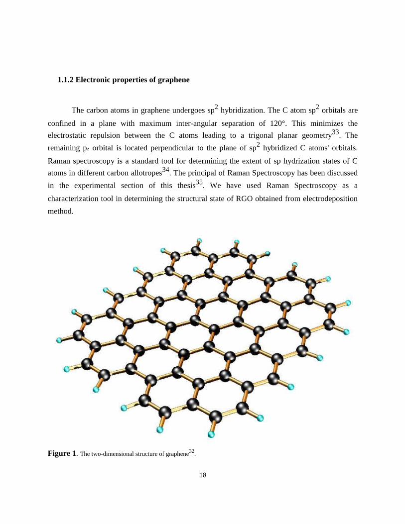
of graphite is called graphene and is shown schematically in figure 1.
18
1.1.2 Electronic properties of graphene
The carbon atoms in graphene undergoes sp2 hybridization. The C atom sp
2 orbitals are
confined in a plane with maximum inter-angular separation of 120°. This minimizes the
electrostatic repulsion between the C atoms leading to a trigonal planar geometry33
. The
remaining pz orbital is located perpendicular to the plane of sp2 hybridized C atoms' orbitals.
Raman spectroscopy is a standard tool for determining the extent of sp hydrization states of C
atoms in different carbon allotropes34
. The principal of Raman Spectroscopy has been discussed
in the experimental section of this thesis35
. We have used Raman Spectroscopy as a
characterization tool in determining the structural state of RGO obtained from electrodeposition
method.
Figure 1. The two-dimensional structure of graphene32
.

19
Fermi Surface of graphene is a six double cone configuration36
. In undoped graphene the
Fermi level is located along the line connecting the midpoints of the six double cones.
Depending on the polarity of the applied field the Fermi surface can be made p-doped or n-
doped. In absence of applied field the density of states at the connecting points between the
Dirac cones and the Fermi level is zero.
Figure 2.The energy, E, for the excitations in graphene as a function of the wave numbers, kx and ky, in the x and y
directions. The black line represents the Fermi energy for an undoped graphene crystal35
.
Graphene contains two edges, the zig-zag and armchair edges. The energy dispersion relation
of edge states of graphene can be found by solving the tight-binding Hamiltonian12
and the relations
are given below,
The C+and C operator are the creation and annihilation operator for states i, j.
H t CiC j h.c
20
The electronic band structure of graphene is a Dirac cone. In order to understand the
electronic properties of any material it is important to understand its energy- momentum
relationship called the band structure37
. The key feature to note is that there exist two bands in
graphene. These are the valance and conduction bands. The valance band is completely filled
while the conduction band is completely empty. This is so as the pz orbitals in graphene are
exactly half-filled. The electrons in graphene behave as massless Dirac particles which in the
electronic band structure appear as gapless excitation along with linear dispersion. Thus,
electrons near the surface in graphene show linear dispersion relation confined in two dimension.
The electronic band structure in graphene is called the Dirac cone structure38
. This makes
intrinsic graphene a metal or zero gap semiconductor. From the dispersion curve of graphene
calculations have been done to show that there is a finite density of state at the Fermi surface for
the zig-zag edge ribbon whereas there is zero density of state for the arm-chair edge ribbon.
1.2 Synthesis of graphene
There are various methods of synthesis of graphene. However, subject to the route of
synthesis the incorporation of defects and the electronic properties vary. Thus, depending on our
synthesis route we may get different property of adhesion for the biosensor film along with
different conduction property of the biosensor film. Hence, we look briefly at the various
synthesis routes available for graphene. In practise we have followed a few selected routes of
synthesis based on their ease and feasibility from point of view of experimental equipment
available.
1.2.1 Exfoliation using scotch tape
Graphene was first isolated by Novoselov and Geim by micromechanical cleavage or
scotch tape peeling of top surface of highly oriented pyrolytic graphite, HOPG39-41
. Pyrolytic
graphite is graphite having strong crystallographic orientation along the c axes42
. HOPG is a highly

21
pure form of pyrolytic graphite. HOPG is obtained by subjecting graphite to annealing and high
compressive stress. The reason for using HOPG as starting material for synthesis of graphene is
because HOPG is a material which has high degree of 3D ordering with lamellar stacking of 2D
planes. The cleavage of HOPG top surface gives a new surface. This new surface is ideally
atomically flat, and hence can be used in STM measurements. Due to cleavage there is formation of
steps on the surface of HOPG. These steps maybe single layered or multi-layered. In our experiment
we have isolated and identified a single layered step edge called a monoatomic step edge by
measuring the z height of the step by atomic force microscope. Single layer steps have step height
close to 0.34 nm. Multilayer or bilayer step has been avoided in our experimental measurements as
step-step interaction has to be taken into account which is not relevant for a single sheet of graphene.
HOPG is nothing but a graphite sample where the angular spread between inter graphite layers is less
than a degree43
. The lower the angular spread the higher the quality of HOPG. Higher quality HOPG
has a larger grain size due to smaller number of steps and hence has a smoother surface. Protocol
used by Novoselov and Geim was as follows: The initial surface peeled from the HOPG was
subjected to repeated cleavage by scotch tape this method can be found in:
You Tube (http://www.youtube.com/watch?v=rphiCdR68TE).
This method is suitable for production of high quality graphene in very poor yields.
Thus this method is not scalable and not suitable for mass production of graphene. Lyding’s
group utilized mechanical cleavage method to isolate graphene monolayers and bilayers with
lateral dimensions in the range of a few nanometers which was deposited on hydrogen
passivated Si(100) surface44
. These works at the beginning of discovery of graphene formed the
basis of investigation of electronic properties of graphene leading to graphene nanoelectronics
development. However, for commercial production better methods giving larger yields of
graphene needed to be devised.

22
1.2.2 Unzipping of CNTs
Unzipping of carbon nanotubes leads to formation of graphene nanoribbons45
. A process
called electrochemical unzipping can convert carbon nanotubes to graphene nanoribbons46
also.
The process of unzipping involves oxidation of carbon nanotubes at a predefined electrochemical
potential followed by unzipping through reduction by chemical agent or electrochemically. A
few layer of graphene sheet has also been obtained by catalytic unzipping of carbon nanotubes
by palladium nanoparticles in oxygen rich medium47
. In the process of unzipping the palladium
nanoparticles act as the unzipping scissors cutting the carbon nanotubes lengthwise. This
synthesis method gives a moderate yield of graphene layers. Synthesis of carbon nanoribbons
from single walled carbon nanotubes is also done by dispersion of the SWCNTs in a mixture of
concentrated nitric and sulphuric acid and ultrasonication48
. Unzipping was also done by
immersing SWCNTs in acetonitrile and sonicating followed by plasma decomposition of CF4 on
the surface of the SWCNTs49
.
1.2.3 Chemical Exfoliation
Another method of synthesis of graphene from graphite is through chemical exfoliation.
For large scale production of graphene two alternatives are possible; large scale growth or large
scale exfoliation. Dispersion of graphite and its exfoliation in organic solvents like N-Methyl-
Pyrrolidone yields concentration of graphene dispersion after exfoliation50
. Choice of organic
solvent depends on the criteria that the energy required for exfoliation of graphite is balanced by
the solvent-graphene interaction. Solvents having surface energy matching that of graphene are
employed for this synthesis route. Graphene can be also be formed by mechanical exfoliation by
wet grinding which leads to delamination of layers and its subsequent dispersion in surfactant
medium to prevent agglomeration. Porphyrin exfoliation of graphite in NMP also leads to
production of graphene51
.
23
1.2.4 Supercritical CO2 method
Another method which is also based on graphene synthesis from graphite is done by
putting natural graphite in a cell and passing supercritical CO2 for thirty minutes through the
cell52
. The products of the reaction can be obtained by passing the output CO2 gas through water
and a surfactant mixture to prevent re-aggregation of graphene sheets.
1.2.5 Annealing graphite in oxygen rich atmosphere
Annealing of graphite in oxygen rich atmosphere having a predefined composition leads
to controlled etching of the hexagonal graphite surfaces. The process can be made to selectively
produce edge states in graphite53
. Selective high etching at defect sites by oxygen flow is done
in this process. From this process predefined structures and networks can be created like
quantum dots and graphene nanoribbons. This method is particularly relevant to future direction
in our research as production of nanoribbons having a particular edge state can lead to formation
of liquid microchannels54
.
1.2.6 Solvothermal Route
It is possible to synthesize single graphene layer by solvothermal method55
. Low
temperature pyrolysis of ethanol and sodium solvothermal mixture produces an intermediate.
The intermediate solid is then washed with water and dried to produce graphene. In the
solvothermal process nanodispersed ethanol undergoes combustion, thermalizing the ethoxide
leading to its decomposition and production of pure graphene. The solvothermal process can also
be carried out by mixing ethanol with sodium borohydride and sodium hydroxide solution. The
reaction product obtained is washed repeatedly with alcohol and water until a neutral pH reading
is registered. The dried product graphene contains many impurities like fullerene and amorphous
carbon. This product is purified by refluxing with nitric acid.
24
1.2.7 Chemical Route
A very high yield, low cost method of synthesis of graphene is through intercalation and
exfoliation of graphene oxide (GO). The chemical route of synthesis of reduced graphene oxide
(RGO) is by chemical reduction of graphene oxide by strong reducing agents like sodium
borohydrate or hydrazine. The use of these reducing agents makes the process toxic and waste
disposal a liability. An alternative to these toxic reagents is the use of citric and ascorbic acid for
reduction of graphene oxide. Graphite nanoplatelets can be obtained from expanded graphite
which is produced by intercalation of different groups into graphite layers by very rapid
evaporation of the intercalate from the underlying layers. An example of this would be rapid
expansion of sulphuric acid intercalated graphite. The resulting material can be ball milled or
exposed to ultrasound to yield nanoplatelets. However this method does not give complete
exfoliation down to single graphene sheets. The thickness of the exfoliated graphite layers
depends on the intercalating agent used as well as the heating temperatures. In a typically
exfoliation process 100 layers of graphene sheets with a thickness of the order of 100 nms is
obtained. A better method of exfoliation would be the synthesis of graphene oxide from graphite
and exfoliation of GO to yield single layer of GO and its subsequent reduction by reducing
agents. It has been shown that GO can be completely exfoliated to give GO single sheets whose
chemical reduction by hydrazine yields graphene sheets. As this method of synthesis is the
easiest and best protocol in wet lab synthesis we have employed a derivative of this method. GO
can be produced by oxidative reaction of graphite by three methods a) Staudenmeier b)
Hummers and c) Brodie56-57
. The three methods differ in the chemical reagents used for
obtaining a oxidizied graphite structure. Physical structure of GO is analogous to graphite both
having a layered structure. However it is easy to differentiate graphite and GO through colour
and texture. GO is lighter in colour than graphite as it is an oxide of graphite. The structure of
GO is that of oxidized graphene sheet having the base plane intercalated with epoxides and
hydroxyl groups in the centre; carbonyls and carboxyl groups at the edges58
. The polar nature of
the oxygen in the oxygen functionalities introduced in the oxidation process makes the GO layers

25
hydrophilic59. Water the oxygen can successfully intercalate between the GO layers. This is a
very important consideration in electrochemical reduction of GO to RGO as aqueous base
electrolyte is used in reduction in our work. Rapid heating of GO causes it to expand and
delaminate due to evaporation of intercalated water at a rapid rate and thermal pyrolysis of the
intercalated oxygen functional groups leading to evolution of gases. This process can produce
single functionalized graphene sheet. However GO being electrically insulating it does not have
any use in electronics as a nano-conductive material. The oxygen functional groups of GO make
the carbon atom in GO sp3 hybridized which leads to its unavailability in bonding with other
atoms. GO is also not stable at high temperatures as the oxygen functional groups may undergo
pyrolysis at elevated temperatures. The reduction of exfoliated GO leads to production of
graphene like individual sheets which are conducting. We have described the Hummers method
in details in the experimental section as a method used by us.
1.2.8 Chemical Vapour Deposition
Chemical vapour deposition or CVD of hydrocarbon on metal surfaces is also a very
standard method of obtaining graphene60
. In this method graphene is grown on metal or carbide
substrates. The underlying 3D substrate provides a scaffold for growth of oriented carbon atoms.
High quality graphene of large area can also be synthesized using CVD technique by
decomposition of selected hydrocarbons such as methane, ethylene, acetylene or benzene on
substrates like Ni, Cu and Cobalt. However apart from research this method is hardly used in
production of graphene due to high cost and stringent experimental conditions control required.
1.2.9 Sublimation (SiC)
Another process is epitaxial growth on SiC and other metal surfaces by the method of
sublimation61
. Single crystal SiC or polycrystalline SiC is heated in a furnace from 1200°C to
1600°C. Higher sublimation rate of Si over C leaves behind C which can rearrange themselves to
produce graphene. This method of production of graphene is very useful in graphene based

26
electronics.
1.3 Wetting property of graphene in relation to its electronic property
Wetting property gives idea about electronic property of the surface62
which is important
in case of a carbon material because depending on the geometry of different carbon surfaces the
electronic property varies which translates in turn to differential hydrogen bonding and Vander
Waals interaction of surface with water molecules leading in turn to different wetting property of
the surface.
The study of wetting property is also important in the case of nano-graphene as Graphene
is the next generation material for electronic fabrication having unique properties like half
integer room temperature quantum hall effect, ten times faster electron transport than that in
silicon due to long range ballistic transport and charge carriers which act like massless Dirac
fermions. To fabricate graphene based electronic devices a photoresist needs to be applied on the
surface of graphene63
. The adhesive property of this coating on the surface of graphene depends
on the wetting property of the surface.
Graphene exposed to air for a long period of time may be susceptible to adsorption of
water molecules present in air. Water adsorbed on the surface of graphene acts as an acceptor
altering the Fermi level position which affects the electronic and transport properties of
graphene64
. However, the adsorption of water on graphene is very much dependent on its
dislocations, defects and edge states65
.
In our work we have used previous reported insights on the differential electronic
properties of the edge states of graphene namely the zig-zag and the arm-chair edges to gauge
that these two edges having different reported electronic states66
should exhibit different
electronic interaction with water molecule which would imply different wetting property of the
edges.

27
Now, a lot of theoretical work has been done on the interaction of these edges with other
molecules67
. However, our work is a unique experimental validation of these theories. The
elegance of our work is that it bypasses the assumptions and shortcomings of the theoretical
works which we will highlight later. We have used the atomic force microscope (AFM) to
characterize these interactions of the edges with water molecules. AFM is a very powerful and
sensitive technique which gives information in nanoscale about differential edge interaction with
water68-69. We have used the atomic force microscope in the frictional microscopy mode
(FFM)70. Work has been done using FFM to map the modified frictional property of a graphene
layer in presence of water molecule.
The ingenuity of the work done by us is that a characterization tool has been used to
glean more information and make interpretations about the scanned system. Recent work
focussed on wetting of graphene shows that wetting property of graphene depends on the number
of layer of graphene sheets in the bulk graphene71
. This has led to fabrication of thin graphene
layer on copper, gold and silicon. The hybrid material is seen to be completely transparent to
graphene with regard to its wetting property. Thus, the future work in this field sees conducting
and impermeable surface coating.
1.4 Wrinkles in graphene sheet
The motivation of study of wrinkling in graphene comes from the effect of wrinkling of
graphene sheet and its effect on the binding affinity of graphene with different drugs and
aromatic compound. Graphene has a vast potential as a drug delivery agent72
. The aspects of
graphene which make it a suitable candidate as a drug delivery agent will be discussed in our
thesis. By conducting AFM study of a graphene surface it was shown that when the graphene
sheet is bend then sp3 nature of the sheet arises and hence one can use graphene as a drug
delivery agent. This curvature effect of graphene surfaces has an impact on the binding affinity
of nucleobases on the surface of graphene74
. To fully understand the binding of an aromatic
compound on graphene the curvature effect has to be taken into account during the modelling.
Our study has an important impact in the understanding of role of binding of graphene to

28
different biological agents. Enzyme binding to graphene surface has important implications in
our later studies of biosensors.
Our study is a first of its kind experimental study of nanographene sheets exhibiting
wrinkling at the surface and at the edges. Apart from the comparative study between wrinkling at
the surface and the edges, the effect of wrinkling on conductivity study has also been done by
doing conductivity mapping using AFM. This method gives a scan image of conductivity of the
entire surface distinguishing the conducting surface from the non-conducting surface. We will
discuss this method further in the experimental section.
1.5 Magnetic and bio-sensing properties of graphene
Our experiments show that both graphene and graphene oxide shows hysteresis loop at
room temperature. However, both graphene and graphene oxide shows diminishing hysteresis
loop as temperature is lowered. This can be explained as follows. Due to the synthesis process
graphene oxide has large number of oxygen and hydroxyl group in it. These functionalized
groups disrupt the sp2 bonded carbon network at many places. On disruption of these bonds
many topological defects are created on the graphene oxide surface which leads to dangling
bonds which have localized moments introduce localized magnetic moment. When graphene
oxide is reduced to reduced graphene oxide these local groups are removed and planarity of the
graphene sheet is restored which leads to diminished moment observed. Hence, we see that
magnetization is proportional to the number of defects in both graphene oxide and graphene. The
role ripple plays in the magnetization of graphene oxide is that due to ripple formation the local
moments of the hydroxyl groups do not interact. However, increase in temperature is found to
flatten out the ripples which leads to interaction between local moments of the hydroxyl group
and thus to higher macroscopic magnetic moment74
. Thus as temperature is increased the
coercivity of graphene and graphene oxide increases. The detailed study of the above
phenomenon will be presented in details by K. Bagani in his thesis. In this thesis we will present

29
the preliminary findings published during the course of this thesis.
Graphene is known to have fast rate of electron transport and very high electronic
conductivity in its pristine state. Thus, graphene is a very promising material for the fabrication
of biosensor75
. Thus, the need of efficient and fast sensor for blood glucose detection as a topic
of research is gaining high importance76
. Due to the present need for a improved glucose
biosensor we have decided to apply graphene electronics to biosensor application. Our approach
to biosensing was the formulation of an amperometric biosensor. Most of the biosensors
available in market today are amperometric biosensors. However due the synthesis route of
graphene which is the Hummer’s method, a chemical synthesis route which introduces a large
number of defects in the graphene structure we have decided to adopt electrochemical synthesis
of RGO77 to detect H2O2.
1.6 Biosensors
The central part of this thesis is the development of biosensors. We have used a glucose
detection biosensor for our basis of study. There are different methods of determining glucose
concentration but the most effective for the purpose of blood glucose detection and monitoring
for diabetes mellitus patients is the development of biosensor based on enzymatic glucose
detection78
.
Glucose level in blood sample can be directly measured by a biosensor by dipping the
biosensor in the sample. This ease of use and measurement speed are the main advantages of
using a biosensor. The bioreceptor in a biosensor is an enzyme. In our study of glucose detection
glucose oxidase has been used but even glucose dehydrogenase can be use. However, better
quality of detection is obtained using glucose oxidase79
.
A transducer holds the capability of conversion of a bio recognition event into a signal
which is measurable. This is usually done by measuring the change happening in a bio receptor
reaction. The biological component activity for a substrate can be gauged by the formation of

30
hydrogen peroxide80
, consumption of oxygen81
, changes in concentration of NADH82
, pH
change83
, temperature change84
, mass change85
, conductivity change or fluorescence86
.
For instance Glucose Oxidase enzyme catalyzes the following reaction:
Glucose + O2 → Gluconic Acid + H2O2 (in presence of GOx)
Measurement of glucose concentration can be done by three different transducers :
Measurement of oxygen concentration by an oxygen sensor
Measurement of change in pH due to production of gluconic acid.
Measurement of concentration of H2O2 by peroxide sensor.
Biology and material science field is merged by the use of nanomaterials in biotechnology.
Nanomaterials are important as biosensors due to their high surface to volume ratio,
compatibility of their size with biomolecules, faster detection limit and biocompatibility. For
instance for the above glucose, cholesterol and uric acid sensor ZnO nanowire has been used as a
substrate87
due to their non-toxicity, biocompatibility, efficient electron transfer between
enzyme and electrode, ease of immobilization of the enzyme and high surface to volume ratio.
Keeping the above points in mind we have fabricated a glucose biosensor in our lab
based on ZnO nanowires. Upon coating with gold shows greater efficiency than standard ZnO
nanowires was observed due to formation of schottky barrier junction88
. Hence, the topic of
different techniques of ensuring effective enzyme loading will be covered. Then this device was
checked for its amperometric performance as a biosensor. Future generation sensors will be
aiming at parallel sensing technique which we shall highlight in future scope section.

31
UAFM for imaging bacteria : Motivation
The main objective of our work with bacteria was to probe the mechanical properties of
bacteria Pseudomonas sp. by contact resonance imaging89
. The fragmentation of these dead
cells was studied using the AFM. It has been observed that with time the cells show multiple
fragmentation sites. Contact resonance imaging help to distinguish the real cell fragments from
the debris of the substrate by mapping the local stiffness of the surface. The importance of
fragmentation studies lies in the fact that it distinguishes between different mechanisms of cell
death. A preliminary study has been performed which can be extended later to include
mechanism of fragmentation.
1.7 Conclusion
Wetting, wrinkle and magnetic property of graphene has been studied and also we shall
present work done on biosensors and UAFM imaging as done during the course of PhD. We
have work with both HOPG and RGO synthesized by exfoliating GO obtained by Hummer’s
method and reducing it using strong reducing agents like hydrazine hydrate. The graphene
obtained by both methods have been used in the study of its properties. During the course of
PhD we have started with glucose oxidase based biosensor. We have fabricated ZnO
electrochemically on ITO substrate. We then extend this work to graphene. We have got some
preliminary results based on graphene synthesized on ITO substrate to obtain non-enzymatic
biosensor. We also image bacteria by contact resonance imaging using AFM.
References :
1) Jannik C. Meyer, A. K. Geim, M. I. Katsnelson, K. S. Novoselov, T. J. Booth & S. Roth,
Nature 446, 60-63 (2007).
2) P. C. Hohenberg, Phys. Rev. 158, 383 (1967)
3) Mermin, N. D. Phys. Rev. 176, 250-254 (1968).

32
4) Philippe Briet, Horia D. Cornean, Baptiste Savoie Annales Henri Poincaré, 13, Issue 1, 1-
40(2012)
5) Kalon, G., Shin, Y. J., & Yang, H Appl. Phys. Lett. 98, 233108 (2011).
6) Yang, Y., Brenner, K., & Murali, R. Carbon, 50, 1727-1733 (2012).
7) Landau, L. D. and Lifshitz, E. M. Statistical Physics, Part I. Pergamon Press, Oxford, 1980.
8) Golberg, D., Bando, Y., Huang, Y., Terao, T., Mitome, M., Tang,
C., Zhi, C., ACS Nano. 4, 2979–2993 (2010).
9) C. Ataca, H. Sahin and S. Ciraci, J. Phys. Chem. C, 116, 8983−8999 (2012).
10) Bibes, M., Villegas, J. & Barthelemy, A. Adv. Phys. 60, 5–84 (2011).
11) Novoselov, K. S. et al. Science 306, 666-669 (2004).
12) Novoselov, K. S. et al. Proc. Natl Acad. Sci. USA 102, 10451-10453 (2005).
13) Novoselov, K. S. et al. Nature 438, 197-200 (2005).
14) Jens Baringhaus et al. Nature (2014).
15) Yuanbo Zhang et al. Nature 438, 201-204 (2005).
16) K. S. Novoselov et al. Nature 438, 197-200 (2005).
17) Kazuyuki Ito, Masayuki Katagiri, Tadashi Sakai, and Yuji Awano, Jpn. J. Appl. Phys. 52,
06GD08 (2013).
18) Wallace, P. R., Phys. Rev. 71, 622 (1947).
19) Ali Shokuhi Rad, Mohsen Jahanshahi, Mehdi Ardjmand, Ali-Akbar Safekordi, Int. J.
Electrochem. Sci., 7 2623 – 2632 (2012).
20) F. Ricciardella, E. Massera, T. Polichetti, M. L. Miglietta, and G. Di Francia, Appl. Phys.
Lett. 104, 183502 (2014).
21) Yuyan Shao, Jun Wang, Hong Wu, Jun Liu, Ilhan A. Aksay, Yuehe Lina, Electroanalysis,

33
22, 1027 – 1036 (2010).
22) Wanda Andreoni et al. Physics and Chemistry of Materials with Low-Dimensional
Structures Volume 23, 291-329 (2000)
23) Kroto, H.W.; et al. Nature 318, 162–163 (1985).
24) Beavers, C.M.; et al. Journal of the American Chemical Society 128 (35), 11352–3 (2006).
25) Wang. X, Li. Qunqing, Xie. Jing, Jin, Zhong, Wang. Jinyong, Li. Yan, Jiang. Kaili, Fan.
Shoushan, Nano Letters 9 (9): 3137–3141 (2009).
26) J W Ding, X H Yan, J X Cao, D L Wang, Y Tang and Q B Yang, J. Phys.: Condens. Matter
15, L439 (2003).
27) "Graphite Statistics and Information". USGS. Retrieved 2009-09-09.
28) Delhaes, P. (2001). Graphite and Precursors. CRC Press. ISBN 90-5699-228-7.
29) Jones, Rick (USAF-Retired) Better Lubricants than Graphite. graflex.org
30) Cristina Gómez-Navarro, R. Thomas Weitz, Alexander M. Bittner, Matteo Scolari, Alf
Mews, Marko Burghard, and Klaus Kern, Nano Letters 7 (11), 3499-3503 (2007)
31) U.S. Geological Survey Minerals Yearbook—2000
32) Andrew R. BarronChristopher E. Hamilton, Graphene. OpenStax CNX. Apr 26, 2012
http://cnx.org/contents/790bacf3-6512-4957-bbed-ac887a4fca7c@4@4.
33) Holleman, A. F.; Wiberg, E. "Inorganic Chemistry" Academic Press: San Diego, 2001. ISBN
0-12-352651-5.
34) Robin W. Havener et al. ACS Nano 6 (1), 373–80 (2011)
35) Gardiner, D.J. (1989). Practical Raman spectroscopy. Springer-Verlag. ISBN 978-0-387-
50254-0.
36) http://www.fom.nl/live/image.pag?objectnumber=127422

34
37) Walter Ashley Harrison (1989). Electronic Structure and the Properties of Solids. Dover
Publications. ISBN 0-486-66021-4.
38) E. Kalesaki, C. Delerue, C. Morais Smith, W. Beugeling, G. Allan, and D. Vanmaekelbergh,
Phys. Rev. X 4, 011010 (2014)
39) Schultz, R. A., et al., Int Jour Fracture 65, 291 (1994).
40) Romero, R., et al., Clay Miner 27, 31 (1992).
41) Novoselov, K. S., et al., PNAS 102, 10451 (2005).
42) K. Matsubara, K. Sugihara, and T. Tsuzuku Phys. Rev. B 41, 969 (1990).
43) IUPAC, Compendium of Chemical Terminology, 2nd ed. (the "Gold Book") (1997).
44) Ritter, K. A. & Lyding, J. W. Nat. Mater. 8, 235–242 (2009).
45) Biwei Xiao, Xifei Li, Xia Li, Biqiong Wang, Craig Langford, Ruying Li, and Xueliang Sun,
The Journal of Physical Chemistry C 118 (2) 881-890 (2014).
46) Dhanraj B. Shinde, Joyashish Debgupta, Ajay Kushwaha, Mohammed Aslam, and
Vijayamohanan K. Pillai, Journal of the American Chemical Society 133 (12) 4168-4171,
(2011).
47) Janowska I., Ersen O., Jacob T., Vennégues P., Bégin D., Ledoux M. J., Pham-Huu, C. Appl.
Catal. A, 371, 22–30 (2009).
48) Izabela Janowska et al. Applied Catalysis A: General 371, 22-30 (2009)
49) Artur Ciesielskia and Paolo Samorì, Chem. Soc. Rev., 43, 381-398 (2014)
50) Ming Zhou et al., Int. J. Electrochem. Sci., 9 810 – 820 (2014)
51) Jianxin Geng, Byung-Seon Kong, Seung Bo Yanga and Hee-Tae Jung, Chem. Commun. ,46,
5091-5093 (2010).
52) Chaiyaporn Wattanaprayoon, “Graphite exfoliation by supercritical carbon dioxide

35
extraction”, Michigan Technological University, Digital Commons@MichiganTech (2011).
53) A. Banerjee and H. Grebel Nanotechnology 19, 365303 (2008).
54) Owen J. Guy, Gregory Burwell, Zari Tehrani, Ambroise Castaing, Kelly-Ann Walker, and
S.H. Doak, Materials Science Forum, 711, 246-252 (2012).
55) Choucair, M., Thordarson, P. & Stride, J. A.. Nat. Nanotechnol. 4, 30–33 (2009).
56) H. L. Poh, F. Šaněk, A. Ambrosi, G. Zhao, Z. Sofer and M. Pumera, Nanoscale, 4, 3515
(2012).
57) Hummers, W. S., Offeman, R. E., Journal of the American Chemical Society 80 (6): 1339
(1958).
58) Pandey, D.; Reifenberger, R.; Piner, R.. Surface Science 602 (9): 1607, (2008).
59) H.P.Boehm, A.Clauss, U Hoffmann. Journal de Chimie Physique (France) Merged with Rev.
Gen. Colloides to form J. Chim. Phys. Rev. Gen. Colloides 58 (12): 110–117 (1960).
60) C. Mattevi, H. Kim and M. Chhowalla, J. Mater. Chem., 21, 3324 (2011).
61) E. Pallecchi, F. Lafont, V. Cavaliere, F. Schopfer, D. Mailly, W. Poirier & A. Ouerghi,
Scientific Reports 4, Article number: 4558
62) Mohammadreza Shahzadeh and Mohammad Sabaeian, AIP Advances 4, 067113 (2014).
63) Kumar et al. Nanoscale Research Letters, 6:390 (2011).
64) Jiří Kysilka, Miroslav Rubeš, Lukáš Grajciar, Petr Nachtigall, and Ota Bludský, J. Phys.
Chem. A, 115 (41),11387–11393 (2011).
65) Oxford Handbook of Nanoscience and Technology: Frontiers and Advances. A.V. Narlikar,
& Y.Y. Fu, Eds. (Oxford Univ. Press, Oxford, 2009).
66) Nakada K., Fujita M., Dresselhaus G. and Dresselhaus M.S. Physical Review B 54 (24):
17954 (1996).

36
67) Zhu Xi., Su, Haibin J. Phys. Chem. C 114 (41): 17257 (2010).
68) S. Banerjee, M. Sardar, N. Gayathri, A. K. Tyagi and Baldev Raj, (2006) 062111.
69) S. Banerjee, M. Sardar, N. Gayathri, A. K. Tyagi and Baldev Raj, (2005) 075418.
70) Varenberg M., Etsion I. and Halperin G., Review of Scientific Instruments 74, 3362-7 (2003)
71) Chih-Jen Shih, Michael S. Strano & Daniel Blankschtein, Nature Materials 12, 866–869
(2013).
72) Sayan Mullick Chowdhury et al., Nanomedicine: Nanotechnology, Biology and Medicine,
11, 109–118 (2015).
73) Swati Panigrahi, Anuradha Bhattacharya, Sangam Banerjee, and Dhananjay Bhattacharyya,
J. Phys. Chem. C, 116 (7), 4374–4379 (2012).
74) K Bagani, A Bhattacharya, J Kaur, AR Chowdhury, B Ghosh, M Sardar, Journal of Applied
Physics 115 (2), 023902 (2014).
75) Tapas Kuilaa, Saswata Bosea, Partha Khanraa, Ananta Kumar Mishrab, Nam Hoon Kimc,
and Joong Hee Lee, Biosensors and Bioelectronics 26, 4637–4648 (2011).
76) F. Davis and S.P.J. Higson, 2 - Electrochemical nanosensors for blood glucose analysis, In
Nanosensors for Chemical and Biological Applications, edited by Kevin C. Honeychurch,
Woodhead Publishing, 2014, Pages 28-53, ISBN 9780857096609.
77) Xu-Yuan Penga, Xiao-Xia Liub, Dermot Diamonda, King Tong Lau Carbon 49, 3488–3496
(2011).
78) Peter Kabasakalian, Sami Kaliney, and Anita Westcot, Clinical Chemistry 20, 606-607
(1974).
79) Jaffari SA, Turner AP. Physiol Meas., 16(1),1-15 (1995).
80) Eun-Hyung Yoo and Soo-Youn Lee, Sensors 10, 4558-4576 (2010).
37
81) Saipeng Yang, Plamen Atanasov, Prof. Ebtisam Wilkins, Annals of Biomedical Engineering
23, 833-839 (1995).
82) Yin Pun Hung, John G. Albeck, Mathew Tantama, and Gary Yellen, Cell Metab. 14(4), 545–
554 (2011). 83) Qingyun Cai, Kefeng Zeng, Chuanmin Ruan, Tejal A. Desai, and Craig A.
Grimes, Anal. Chem., 76 (14), 4038–4043 (2004). 84) Avula M., Engineering in Medicine and
Biology Society,EMBC, 2011 Annual International Conference of the IEEE. 85) Nor M.M.,
Semiconductor Electronics (ICSE), 2012 10th IEEE International Conference.
86) David C. Klonof, Journal of Diabetes Science and Technology 6, 1242-1250 (2012). 87)
Yang Lei, Ning Luo, Xiaoqin Yan, Yanguang Zhao, Gong Zhanga and Yue Zhang Nanoscale 4,
3438-3443 (2012). 88) Song Liu and Xuefeng Guo, NPG Asia Materials 4, e23 (2012) 89) Mark
F. Murphy,Michael J. Lalor,Francis C.R. Manning,Francis Lilley,Steven R. Crosby,Catherine
Randall,David R. Burton, Microscopy Research and Technique 69, 757–765 (2006)

38
Chapter 2
Experimental Methods
2.1 Introduction
In this chapter we shall describe the experimental methods such as: sample preparation,
experimental techniques and the analysis scheme used by us for this thesis. These include
preparation of graphene from highly oriented pyrolytic graphite (HOPG), zinc oxide nanorods
(ZnO NRs), chemical synthesis of graphene oxide (GO) and reduced graphene oxide (RGO). In
this chapter we shall also discuss techniques like operation of AFM in different modes and
different measurement modes of electrochemical workstation. Further discussions will be done
on the analysis scheme adopted in interpreting our experimental results using AFM and
electrochemical workstation.
2.1.1 Sample preparation
1) Synthesis of graphene by exfoliation.
The loosely held nano-graphene ribbon on HOPG substrate was made measurement ready
by peeling the top surface of the HOPG using a scotch tape to expose freshly cleaved edges of
nanoribbons. Frictional force measurement and conductivity mapping was done on the cleaved
surface of the HOPG by using a NT-MDT atomic force microscope. For the peeling process to
be smooth without resulting in cleavage of the entire HOPG substrate in half, there has to be a
minimum thickness of the substrate employed. Very thin substrates do not yield good results
with the above method. The cleavage of the HOPG using scotch tape results in the topmost layer
of the HOPG being more loosely held than the underlying layers which makes it suitable to study
processes occurring in nanographene. Successive layers were peeled and imaged using AFM to
optimize result. Wetting properties of graphene was studied using peeled HOPG by an AFM
(Atomic Force Microscope) in FFM (Frictional Force Microscopy) mode. Conductivity of

39
graphene nanoribbons were studied in conductivity mapping mode using AFM on a freshly
peeled HOPG substrate surface.
2) Synthesis of Graphene Oxide (GO) and Reduced Graphene Oxide (RGO) by
chemical and electrochemical route.
GO was synthesized by Hummer’s method which is a chemical route of synthesis. The
resulting brown GO was reduced by hydrazine hydrate to yield RGO. This process yields RGO
in good quantity but the quality of the sample is poor containing many defects in the form of
carboxyl and carbonyl bonds. The principle of Hummer’s method is to intercalate oxygen
containing functional groups between graphite layers leading to an increased interlayer
separation. The oxygen containing functional groups are then reduced to yield a graphene like
structure, the RGO. The magnetic properties of the sample are studied using SQUID
magnetometer. The RGO obtained was characterized by RAMAN spectroscopy.
For the synthesis of RGO we used the following protocol: 2 gms of graphite powder and
1 gm of NaNO3 was weighed and kept aside. 46 ml of H2SO4 (Sulfuric acid) as available which
was 98 percent purity was taken. An ice bath was made using crushed ice in a thermocol box and
temperature was maintained at around 0°C. At 0°C 46 ml of H2SO4 was added to 2 gms of
graphite powder and 1 gm of NaNO3 was slowly added to the mixture for 30 minutes. This
mixture was stirred by placing the setup on a stirrer using magnetic beads for stirring. While
stirring 6 gms of KMnO4 was added for an hour and care was taken that the temperature does not
exceed 20°C. The ice bath was removed and the temperature was allowed to come to 35°C. 30
minutes after this 92 ml of water was added slowly for 40 minutes. After this 280 ml of water
was heated to 40-60°C and then added. Then 30 percent H2O2 was added to the mixture until the
colour changed from brown to sunset yellow and evolution of fumes ceased. The remaining
solution was filtered and centrifuged and washed repeatedly with water until the pH of the
supernatant became neutral.

40
The above method is known as the Hummers method1. In this method though
permanganate is the oxidizing agent the active species is in fact diamanganese heptoxide. The
product obtained from the above process is called graphene oxide or GO. RGO is synthesized
from GO by refluxing the obtained GO in a solution of 32.1 mM hydrazine hydrate in an oil bath
at 100°C for 24 hours at the end of which RGO precipitated out of the solution and was washed
and filtered and dried.
For obtaining thin film of RGO on Indium Tin Oxide (ITO) the process carried out by us
is as follows. A suspension of graphene oxide and K2HPO4 (Dipotassium Hydrogen Phosphate)
is taken as the supporting electrolyte. The pH of the solution is adjusted to 5. ITO coated glass
slides are mounted on the working electrode and a cyclic voltammogram (CV) from -1.4 to 0
Volts is given for 30 cycles to obtain a polished layer of reduced graphene oxide, RGO on the
ITO surface. Calomel reference electrode and platinum wire counter electrode are used. The CV
plot is shown in fig. 1
Figure 1. CV plot of GO in PBS for 30 cycles
3) ZnO NR prepared by electrodeposition.
ZnO NR was prepared by electrodeposition on a conducting ITO (Indium Tin Oxide)

41
coated glass substrate. A conventional three electrode configuration was adopted with Ag/AgCl
as the reference electrode, a Pt wire (0.5mm) as counter electrode and an Indium Tin Oxide
(ITO) coated glass substrate (3mm X 3mm) as the working electrode. The glass slide was held
by a steel holder which is dipped into Zinc nitrate hexahydrate Zn(NO3)2:6H2O and
Hexamethylenetetramine (HMT, 99 %) in the ratio of 1:1 by concentration (20 mM). The ZnO
NR arrays were prepared by a simple one step electrochemical process controlled by
electrochemical workstation (CHI 660C, CH Instruments, Inc.). The electrolyte was 30mL
aqueous solution of 20mM Zn(NO3)2 and 20mM HMT. After immersing the sample in the
electrolyte no external voltage was passed for 15 seconds to allow the open circuit voltage
between the cathode and anode stabilize. The deposition was carried out at 80oC at an applied
negative voltage of -0.8V for 7000s. After 7000s ZnO NRs arrays (whitish color) were formed
on ITO substrate which was washed with distilled water to remove un-reacted species from the
surface.
Figure 2. CV of ITO in Zinc Nitrate and HMT solution indicating the deposition potential to be -
0.8 V.
The synthesized ZnO is dried and this is used as a template for fabrication of glucose
biosensor. GOx (Glucose Oxidase) enzyme is used as a catalyst in the glucose biosensor. Method
of synthesis of Glucose biosensor will be presented in Chapter 5.

42
4) Bacteria on TiO2 substrate.
In the present investigation, a thin film of TiO2 was prepared by anodizing commercially
pure titanium coupons (2 cm X 2 cm) in an acid bath (nitric acid 400 g/l added to hydrofluoric
acid 40 g/l added to water) and then ultrasonically cleaned using soap solution to remove all
traces of acid from the surface. The coupons were then washed in running water and finally
rinsed in distilled water and air-dried. Anodization was carried out at 25°C in orthophosphoric
acid (30 g/l) for 48 h at 30 V. Pseudomonas sp. had been used as test micro-organism to study
the elastic property of bacteria to differentiate it from its surrounding.
2.2 Experimental techniques
a) Atomic Force Microscopy.
An AFM operation is similar to operation of gramophone stylus2. The tip scans the
surface feeding information about the surface topography to a photodetector by laser light
reflected off the back of the cantilever containing a sharp tip. The deflection of the cantilever is
measured using laser deflection technique. The cantilever deflection error signal is given as an
output to the negative feedback control unit. The feedback control unit is able to control the z-
position of the piezo on basis of the cantilever deflection signal error. The mode of operation of
AFM can be “Constant force (contact mode)” and “Constant height
(non-contact mode)”. The feedback adjusts the height of obtained sample placed under the
cantilever tip based on the cantilever deflection signal error, however if the feedback gain is not
high the cantilever stays at almost “constant height” and collection of cantilever deflection data
takes place. When the feedback gain is high, the height of the piezo changes to keep the

43
cantilever deflection almost constant, hence, the force is constant and the height change of the
piezo is recorded by the system3.
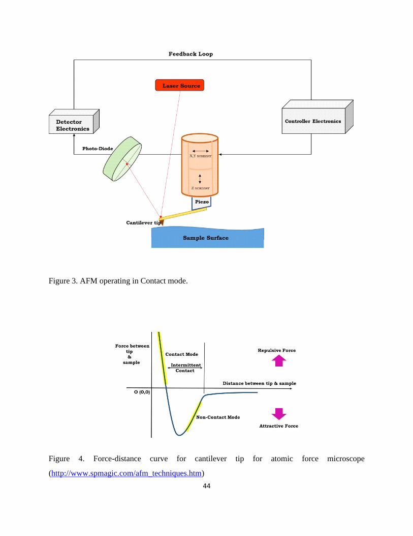
2.21 Contact mode of operation.
We briefly discuss the principle of operation of the AFM in contact mode. The sample is
first mounted on a PZT scanner which is equipped with individual electrodes to scan the x-y in
raster pattern and move the sample in z direction. A very sharp tip of a flexible cantilever is
brought close to sample surface until it is in contact with the sample surface. As the sample
moves under the tip, sample surface features cause the cantilever tip to deflect in vertical and
lateral directions. A laser beam from a 5mW laser power source falls on the back of the
cantilever tip which is highly polished and reflects back to the photo-diode. The photo-diode is
split into four quadrants, two positive quadrants and two negative quadrants. The difference in
signal from the positive and negative quadrant of the photo-diode gives rise to the AFM signal
which is a sensitive way of measuring the cantilever’s vertical deflection. Undulations on the
surface of the sample which are due to topographic features present on it cause the tip to be
deflected in the vertical direction as the sample is scanned. In the “contact mode” of operation of
the AFM the applied normal force on the sample surface while imaging the topography has to be
kept constant, a feedback circuit system modulates the voltage applied on the PZT scanner which
adjusts the height of the PZT, such that the cantilever vertical deflection is held constant during a
scan. The height variation of the PZT is a direct indication of sample surface topography4-6
. In
this mode the feedback gain is kept high and the AFM is operated in the repulsive region of the
cantilever’s force-distance curve as seen by the distance between the tip and sample in fig. 4
44
Figure 3. AFM operating in Contact mode.
Figure 4. Force-distance curve for cantilever tip for atomic force microscope
(http://www.spmagic.com/afm_techniques.htm)

45
2.2.2 Tapping Mode.
In the tapping or dynamic mode of operation, the tip and the sample surface are brought
in close proximity of each other without actually touching each other. During scanning over the
sample surface in the tapping mode, the cantilever tip is sinusoidal vibrated at its resonance
frequency. The oscillating tip lightly taps the sample surface at frequency of resonance of the
cantilever. Constant oscillating amplitude is introduced in the vertical direction in which a
feedback loop is used to keep the average normal force as constant. The amplitude of oscillation
is kept not large enough to avoid the tip getting stuck on the surface of the sample due to
presence of adhesive forces of attraction. The tapping modes is usually employed when there is a
fear of the sample surface getting damaged due to the cantilever tip dragging over it in a contact
mode operation and thus prevent soft samples like biological membranes etc., from damage7.
2.2.3 Frictional Force Microscopy.
Frictional force on a sample surface can also be measured using an AFM where the two
right and two left quadrant of the photo-detector are used. In FFM mode scanning is done
perpendicular to the long axis of the cantilever. Frictional force existing between the tip and the
sample surface will cause the twisting of the cantilever during a scan. Hence, the laser beam will
be deflected laterally in contrast to the deflection of a laser beam deflecting vertically for an
untwisted cantilever measuring surface topography. This gives a measurable intensity difference
between light falling on the left and right side of the photo-detector. This intensity difference can
be converted into a 2D map of the frictional force8-10
. In the frictional force microscopic
technique, one can measure simultaneously both the topography and the frictional property by
recording the current signals Iver proportional to normal bending of the cantilever (which carries
the AFM tip) and Itor which is proportional to torsional bending of the cantilever simultaneously.
The current signals Iver represent the topographical height distribution and the current signals Itor

46
represent the frictional component of the sample surface in that region. This is described
schematically in figure 3.
Figure 3. Schematic diagram of the vertical and torsional bending of the cantilever due to tip-surface interaction.
The photodiode shows four quadrants A, B, C and D. The reflected laser light from the cantilever have vertical
motion on the photodiode due to vertical bending and lateral motion due to torsional bending of the cantilever. [1]
Figure 4. Schematic illustration of Itor due to the torsional bending of the cantilever for the forward and reverse
directions of the scan showing sign reversal of Itor . For the respective scan directions we have plotted a histogram of
Itor versus N (N is number of points per Itor ). [Note: the maxima of Itor become minima on reversal of scan direction
leading to contrast inversion in FFM images.] [ Adapted from Applied Physics Letters 86 (21), 211913]

47
In figure 4 we show schematically the data analysis scheme adopted in this thesis. The
current signal Itor due to the torsional bending of the cantilever during a line scan along the
forward (left to right) and backward (right to left) directions is shown. Since the torsional angle
(β) changes sign when moving in the opposite direction the current signal Itor also changes sign.
We have also shown in figure 4 a histogram of the torsional bending of the cantilever
proportional to the current Itor . We would like to mention that throughout our experiment on all
the samples the position of the laser beam on the cantilever was kept on the same spot and the
scan speeds were also maintained the same. This is very important since we know that variation
of the position of the laser beam on the cantilever determines the amplitude of bending of the
cantilever.
We observed contrast inversion when the scanning direction is reversed, as explained
schematically in figure. One can quantitatively obtain the overall change in the frictional
property by plotting a histogram
for both the scan directions as described schematically
in figure 4. The average value Itor,avg is defined as
Itor,avg = [Itor,max(+) + |Itor,max(−)|]/2, (1)
where Itor,max(+) and Itor,max(−) are the values of Itor each corresponding to the maximum N which is
the number of points in the histogram for the forward and reverse scan directions respectively.
Itor,avg is proportional to the frictional force.

48
2.2.4 Ultrasonic Force Microscopy (UFM) /Atomic Force Acoustic Microscopy (AFAM).
Figure 5. (a) Schematic diagram of the experimental setup of atomic force acoustic microscopy (AFAM) and
ultrasonic force microscopy (UFM). (b) Schematically, the resonance curve and the shift of the resonance curve for
higher and lower effective elastic constant regions (marked as soft and stiff) [Adapted with permission from Applied
Physics Letters 86 (21), 211913].
Atomic force microscope (AFM) with its innovative modifications has become one of the
most important tools to study local surface properties at nanoscale level. One of the important
properties of sample surfaces is its local elastic (stiffness) modulus. Some of the modified
techniques used to obtain the local elastic properties are force modulation microscopy, force
versus distance curve, nanoindentation, ultrasonic force microscopy (UFM), scanning
microdeformation microscopy, and measurement of contact resonances. In the UFM technique,
the cantilever carrying the probing tip is excited by a piezo attached to the cantilever as shown in
Fig. 5(a). The probing tip is in contact with the sample surface in a constant force mode and one
measures the contact resonance curve of the cantilever. This method depends on detection of

49
cantilever deflections in response to vibrations which are ultrasonic that causes periodic
indentation of the sample surface at frequencies which are very much greater than cantilever
resonance frequencies.
In Fig. 5(b) and in more detail in figure 6 we also show schematically the tip–sample
contact resonance curve showing maximum amplitude of vibration at its coupled resonance
frequency. If the tip is in contact with a stiff region on the surface of the sample the peak
frequency and the amplitude of the contact resonance curve increases. On the other hand if the
tip is in contact with a soft region on the surface of the sample, the peak frequency and the
amplitude of the contact resonance curve decreases and the full width at half maximum of the
curve increases generally. If we select the operating frequency above the peak frequency value
and monitor its amplitude using a lock-in amplifier then when the tip moves to a stiff region. the
amplitude of oscillation of the cantilever will increase because the curve will move toward
higher frequency with an increase in its amplitude. If the tip moves to a soft region then the
opposite happens i.e., the contact resonance curve moves toward lower frequency and the
amplitude of cantilever oscillation decreases. Hence, if the highest amplitude of the cantilever
oscillation is designated as the brightest (white) on the grey scale image and the lowest
amplitude as the darkest (black), then by monitoring the amplitude of oscillation of the cantilever
one can distinguish the stiffer region and the softer region on the surface from the image.
On the other hand if we choose the operating frequency is lower than the contact
resonance peak value then the stiffer region on the sample surface will be shown as darker areas
and the softer region as brighter areas in the UFM images. Thus one can observe contrast
inversion in the image depending on the choice of the operating frequency. In the UFM
techniques, the behavior of the resonance curve will be dictated by the effective local stiffness
constant. In AFAM mode one bonds the sample onto an ultrasoninc
transducer and the rest of the operation is similar to UFM
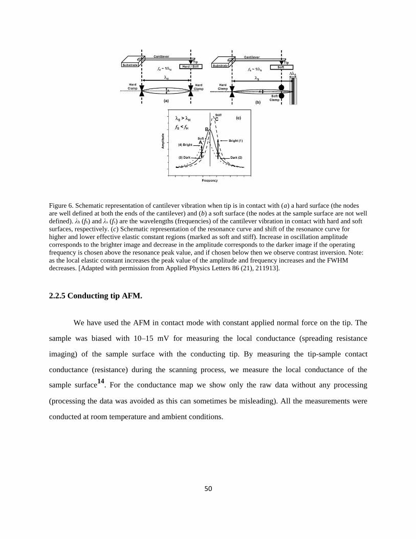
50
Figure 6. Schematic representation of cantilever vibration when tip is in contact with (a) a hard surface (the nodes
are well defined at both the ends of the cantilever) and (b) a soft surface (the nodes at the sample surface are not well
defined). λh (fh) and λs (fs) are the wavelengths (frequencies) of the cantilever vibration in contact with hard and soft
surfaces, respectively. (c) Schematic representation of the resonance curve and shift of the resonance curve for
higher and lower effective elastic constant regions (marked as soft and stiff). Increase in oscillation amplitude
corresponds to the brighter image and decrease in the amplitude corresponds to the darker image if the operating
frequency is chosen above the resonance peak value, and if chosen below then we observe contrast inversion. Note:
as the local elastic constant increases the peak value of the amplitude and frequency increases and the FWHM
decreases. [Adapted with permission from Applied Physics Letters 86 (21), 211913].
2.2.5 Conducting tip AFM.
We have used the AFM in contact mode with constant applied normal force on the tip. The
sample was biased with 10–15 mV for measuring the local conductance (spreading resistance
imaging) of the sample surface with the conducting tip. By measuring the tip-sample contact
conductance (resistance) during the scanning process, we measure the local conductance of the
sample surface14
. For the conductance map we show only the raw data without any processing
(processing the data was avoided as this can sometimes be misleading). All the measurements were
conducted at room temperature and ambient conditions.
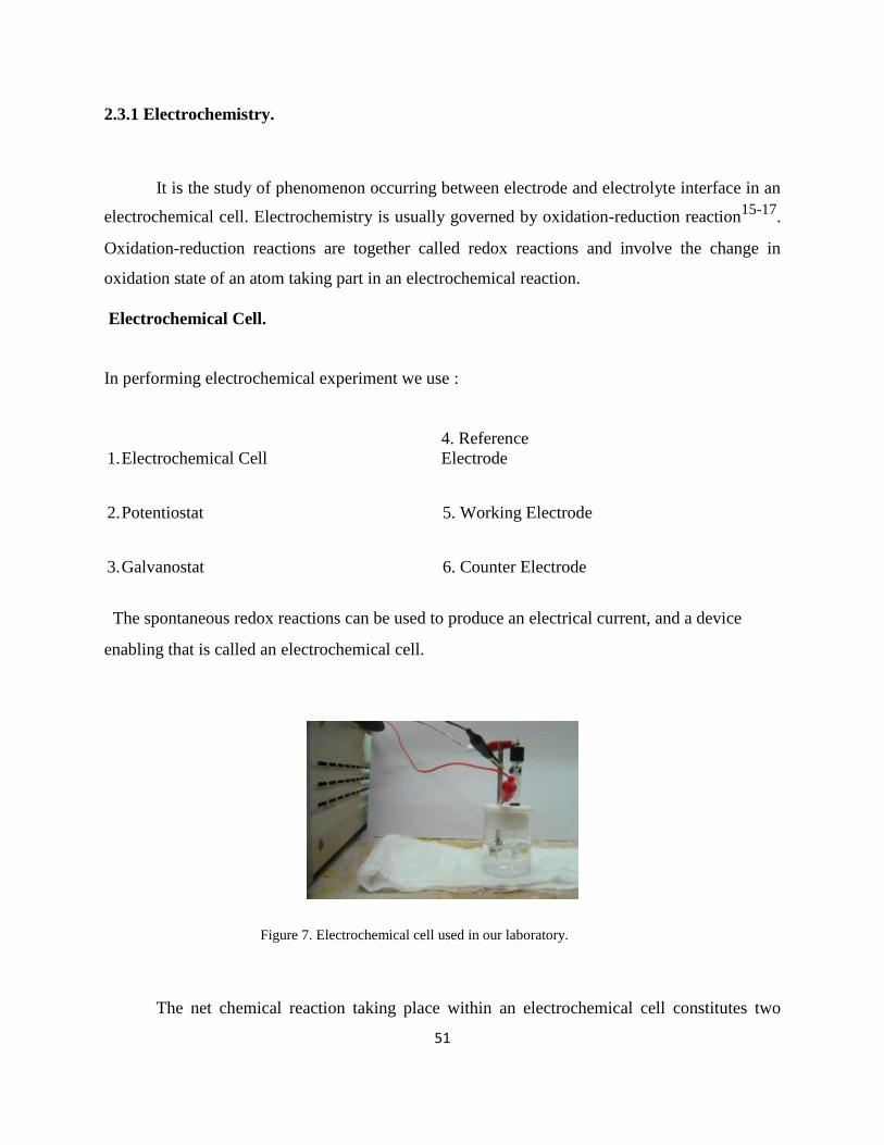
51
2.3.1 Electrochemistry.
It is the study of phenomenon occurring between electrode and electrolyte interface in an
electrochemical cell. Electrochemistry is usually governed by oxidation-reduction reaction15-17
.
Oxidation-reduction reactions are together called redox reactions and involve the change in
oxidation state of an atom taking part in an electrochemical reaction.
Electrochemical Cell.
In performing electrochemical experiment we use :
1. Electrochemical Cell 4. Reference
Electrode
2. Potentiostat 5. Working Electrode
3. Galvanostat 6. Counter Electrode
The spontaneous redox reactions can be used to produce an electrical current, and a device
enabling that is called an electrochemical cell.
Figure 7. Electrochemical cell used in our laboratory.
The net chemical reaction taking place within an electrochemical cell constitutes two

52
independent half reactions. These reactions give a picture of the changes occurring at the two
electrodes. The electrochemical reactions within a cell thus occurs at the two electrodes, one
called the working electrode which operates in conjunction with an electrode which is an
approximation of an ideal non-polarizable electrode of fixed known potential called the reference
electrode. In our electrochemical cell current is passed between a working and a counter
electrode.
These three electrodes are placed in a small glass beaker having a cap with three
openings for the three electrodes in a conventional three electrode electrochemical cell. These
three elecrodes are described in the subsections below.
2.3.2 Potentiostat.
A potentiostat is an instrument which measures and controls the voltage between a
working electrode and a reference electrode18-20
. A potentiostat works with three electrodes
immersed, working, reference and counter electrodes within a electrolyte. The potentiostat has
three electrode arrangement as the potential and current at the working electrode can be
measured irrespective of the other two electrode potentials contribution or interference.
There are three primary components of a potentiostat,
Control Amplifier : It supplies the power to maintain the potential difference between the
reference and working electrode.
Electrometer : It measures the potential difference between reference and working
electrode.
Current to voltage converter: It measures the current between counter and working
electrode.

53
2.3.3 Galvanostat.
It is a measuring and control device which is capable of maintaining the current through
an electrochemical cell as constant in coulometric titrations, disregarding the changes in load. In
the galvanostat there is a high voltage source producing the voltage V which is constant with a
resistance Rs in series. In order to maintain a constant current through the load resistance the
series resistance has to be much higher than the load resistance Rload.
= V/(Rs + Rload)
V/ Rs
If Rs >> Rload
2.3.4 Reference Electrode.
A reference electrode is a stable electrode having a well-known electrode potential. The
relatively high stability of the electrode potential is obtained by using a redox system with
saturated concentrations of each of the redox reactions’ participants. There are different ways in
which a reference electrode can be used. In most cases reference electrode is used as a half cell
in an electrochemical cell allowing the potential of the other half cell to be determined21-22
.
2.3.4.1 Ag/AgCl reference elecrode.
This is a type of reference electrode commonly used in electrochemical measurements.
This electrode is a type of redox electrode with reaction between the Ag and its salt AgCl.
The equations of silver chloride reference electrode are as follows:
Ag+ + e
- ↔ Ag(s)

54
AgCl(s) ↔ Ag+ + Cl
-
Hence, the overall reaction combining the above two reactions can be written as,
AgCl(s) + e- ↔ Ag(s) + Cl
-
This is a fast electrode kinetics characterized reaction. The standard electrode potential of
Silver chloride electrode vs SHE (Standard Hydrogen Electrode) at 25°C is 0.23V.
2.3.4.2 Calomel reference electrode.
Calomel reference electrode is electrode based on reaction between mercury, Hg and
Mercury Chloride, Hg2Cl2. The aqueous solution in contact with mercury and mercury chloride
or calomel is a saturated potassium chloride solution. The calomel is linked by a porous frit to
the solution of potassium chloride in which the other electrode is immersed.
The redox reaction of the electrode is as follows:
Hg22+
+ 2e- ↔ 2Hg(l)
Hg2Cl2(s) ↔ Hg22+
(l) + 2Cl-(l)
Hence, the overall reaction combining the above two reactions can be written as,
Hg2Cl2(s) + 2e
- ↔ 2Hg(l) + 2Cl
-(l)
When it is saturated the standard electrode potential of Calomel electrode vs SHE at 25°C is
0.2444 V.

55
2.3.5 Counter Electrode.
It is an electrode used in a voltammetric reaction in an electrochemical cell where current
is expected to flow. In a two electrode setup a predefined potential is applied between counter
and working electrode and all other variables are measured. The counter and the working
electrode have an anode cathode relationship i.e., one acts as the anode while the other acts as the
cathode and vice-versa. When a three electrode setup is used the counter electrode along with the
working electrode establishes a circuit over which current is measured or applied. In this setup,
the potential at the counter electrode is usually not measured. The potential at the counter
electrode is adjusted to balance the reaction occurring at the working electrode. This arrangement
allows the measurement of the potential of the working electrode w.r.t reference electrode
without compromising the integrity of the reference electrode by passing a current through it.
Counter electrodes are usually made of inert materials.
2.3.5.1 Platinum counter Electrode.
The counter electrode we have used is a platinum counter electrode. This is an inert
electrode which is not affected by the chemical reaction occurring at the counter electrode.
In our case we have observed that on continued use of the counter electrode a brown layer coats
the platinum wire. In that case due to presence of impurity reaction is interrupted. Thus the Pt
wire is cleaned using a dilute nitric acid solution.
2.3.6 Working Electrode.
The working electrode is the electrode in which the reaction of interest is occurring. In
our case the working electrode is an ITO coated glass slide held into the solution by steel clips.
In case of fabrication of ZnO from zinc nitrate, the reaction occurring at the working electrode is
as follows :
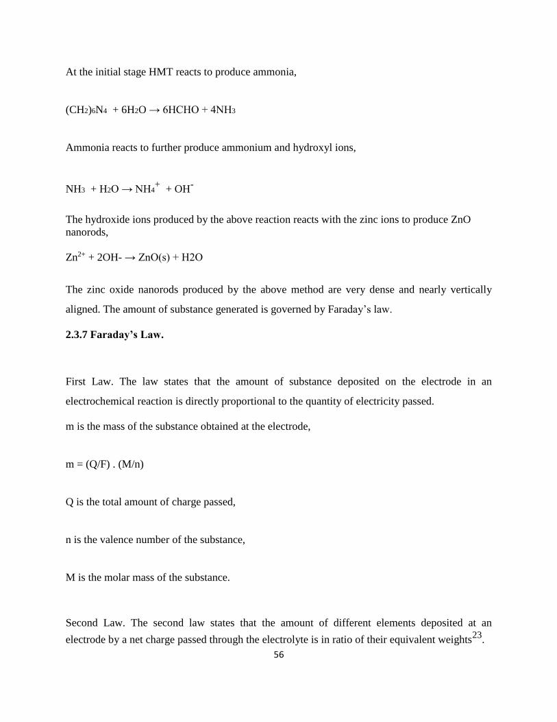
56
At the initial stage HMT reacts to produce ammonia,
(CH2)6N4 + 6H2O → 6HCHO + 4NH3
Ammonia reacts to further produce ammonium and hydroxyl ions,
NH3 + H2O → NH4+ + OH
-
The hydroxide ions produced by the above reaction reacts with the zinc ions to produce ZnO
nanorods,
Zn2+ + 2OH- → ZnO(s) + H2O
The zinc oxide nanorods produced by the above method are very dense and nearly vertically
aligned. The amount of substance generated is governed by Faraday’s law.
2.3.7 Faraday’s Law.
First Law. The law states that the amount of substance deposited on the electrode in an
electrochemical reaction is directly proportional to the quantity of electricity passed.
m is the mass of the substance obtained at the electrode,
m = (Q/F) . (M/n)
Q is the total amount of charge passed,
n is the valence number of the substance,
M is the molar mass of the substance.
Second Law. The second law states that the amount of different elements deposited at an
electrode by a net charge passed through the electrolyte is in ratio of their equivalent weights23
.
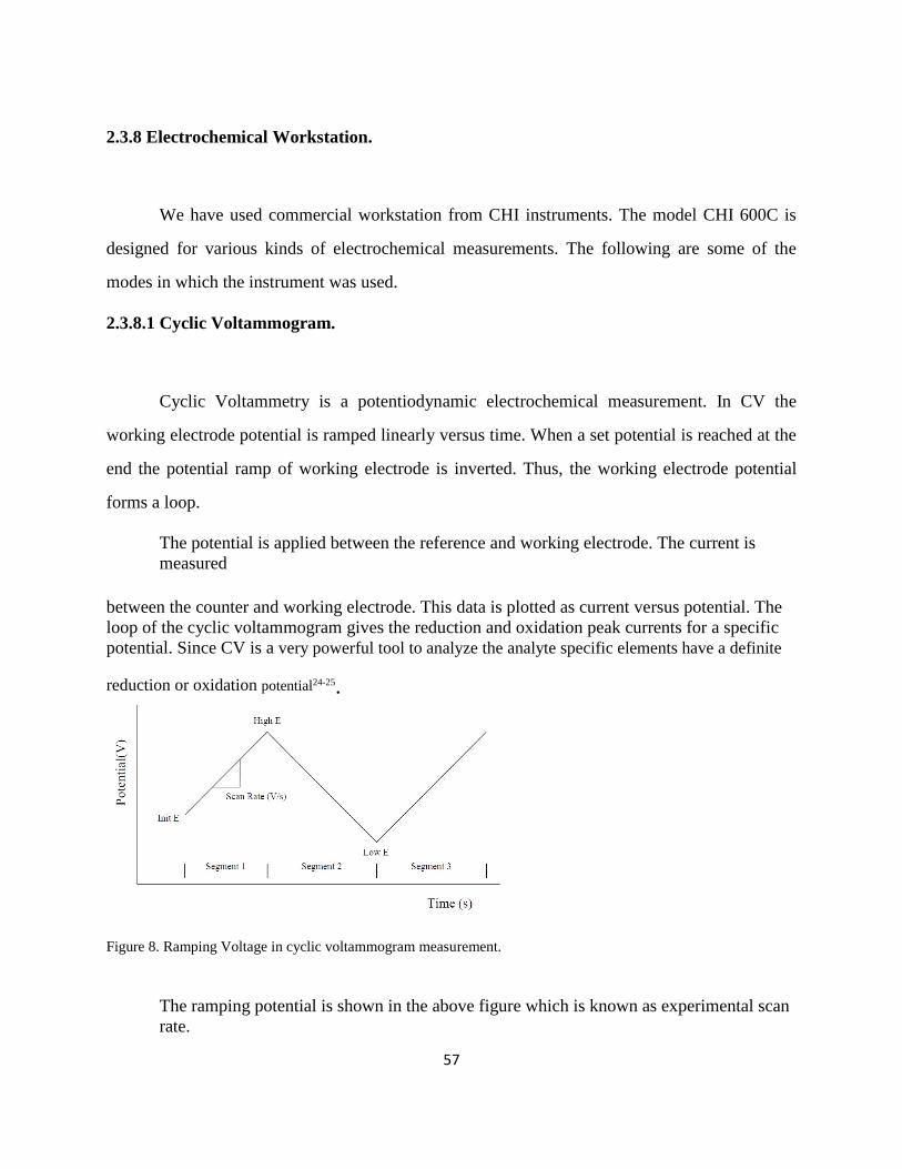
57
2.3.8 Electrochemical Workstation.
We have used commercial workstation from CHI instruments. The model CHI 600C is
designed for various kinds of electrochemical measurements. The following are some of the
modes in which the instrument was used.
2.3.8.1 Cyclic Voltammogram.
Cyclic Voltammetry is a potentiodynamic electrochemical measurement. In CV the
working electrode potential is ramped linearly versus time. When a set potential is reached at the
end the potential ramp of working electrode is inverted. Thus, the working electrode potential
forms a loop.
The potential is applied between the reference and working electrode. The current is
measured
between the counter and working electrode. This data is plotted as current versus potential. The
loop of the cyclic voltammogram gives the reduction and oxidation peak currents for a specific
potential. Since CV is a very powerful tool to analyze the analyte specific elements have a definite
reduction or oxidation potential24-25.
Figure 8. Ramping Voltage in cyclic voltammogram measurement.
The ramping potential is shown in the above figure which is known as experimental scan
rate.

58
2.3.8.2 Amperometric Response.
In amperometric I-t curve a constant potential is applied against which the current is
recorded as a function of time. The graphical plot of the above scheme for our CHI600C is
shown below.
Figure 9. Schematic of applied potential vs time in amperometric i-t curve.
.
2.3.8.3 Electrochemical Impedance Spectoscopy.
EIS is known to measure the dielectric properties of a medium as a function of
frequency. It works on the principle of external field interaction with the sample’s internal dipole
moment. In our case we have used it to characterize the electrochemical system of glucose
biosensor and PBS (Phosphate Buffer Solution) by measuring the impedance of the system over
a range of frequencies.
An electrolyte electrode interface acts as a capacitance called electrical double layer
capacitance. The equivalent circuit for a redox reaction is a capacitance in parallel with the
charge transfer resistance. We have calculated this charge transfer resistance from the Nyquist
plot. Nyquist plot is a parametric plot of frequency response26-28

59
2.4 Basic principle of RAMAN spectroscopy.
We have used Raman spectroscopy to characterize GO and RGO samples. RAMAN
spectroscopy of RGO shows two distinct peaks with one peak larger than the other. We have
done Raman spectroscopy on RGO film and obtained the standard double peak common to
graphene samples in which G peak for multilayer graphene is at 1580 cm-1
which shows the
partial reduction of
Figure 10. The Raman peak for graphite, GO and RGO and graphene.
graphene oxide by electrochemical methods. The D peak of RGO originates from defect induced
breathing of sp2 modes
29.
2.5 Basic principle of SQUID magnetometer.
In SQUID Josephson junction is formed by separating two superconducting regions by a
thin insulating layer. In a SQUID magnetometer parallel Josephson’s junction is employed. The
electrical current density between two superconductors separated by a thin insulating layer
depends on the phase difference between the wavefunctions. The derivative of this phase
difference w.r.t time is related to voltage across the junction. In superconducting ring with one or
two insulating layers, the phase difference also depends on the magnetic flux within this ring.

60
Such a device can be used to convert magnetic flux to electric voltage. This is the basic working
principle of a SQUID magnetometer. The sample is moved up and down to produce alternating
magnetic flux through the pickup coil. The magnetic signature of the sample is obtained by a
superconducting pick-up coil.
In our study a commercial SQUID magnetometer (Quantum Design, USA) has been used to
study the behaviour of GO and RGO.
References:
1) Ji Chen, Bowen Yao, Chun Li, Gaoquan Shi, Carbon 64, 225–229 (2013)
2) Binnig, G.; Smith, D. P. E. Review of Scientific Instruments 57, 1688 (1986)
3) Giessibl, F. J.; Trafas, B. M. (1 January 1994)Review of Scientific Instruments 65 (1923)
4) Yao, X., M. Jericho, D. Pink, and T. Beveridge. J. Bacteriol. 181, 6865-6875 (1999)
5) Xu, W., P. J. Mulhern, B. L. Blackford, M. H. Jericho, M. Firtel, and T. J. Beveridge. J.
Bacteriol. 178, 3106-3112 (1996)
6) Wetzer, B., D. Pum, and U. B. Sleytr. . J. Struct. Biol. 119, 123-128 (1997)
7) Butt HJ. Biophys J., 63(2), 578–582 (1992)
52
8) M Teresa Cuberes and Juan J Martinez J. Phys.: Conf. Ser. 61, 224(2007)
9) B. Bhushan, Handbook of Micro/Nanotribology (CRC Press, New York, 1995)
10) M. Mate, G.M. McClelland, R. Erlandsson and S. Chiang, Phys. Rev. Lett. 59, 1942(1987)
11) M. Scherge and J.A. Schaefer, Tribol. Lett. 4, 37(1998)
12) S. Jang and J. Tichy, Tribology 119, 626 (1997)
13) C. Dorier and J. Tichy, J. Non-Newtonian Fluid Mech. 45, 291 (1992)

61
14) Terunobu Akiyama et al. Jpn. J. Appl. Phys. 43, 3865 (2004)
15) Hudlický, Miloš (1996). Reductions in Organic Chemistry. Washington, D.C.: American
Chemical
Society. p. 429. ISBN 0-8412-3344-6
16) Hudlický, Miloš (1990). Oxidations in Organic Chemistry. Washington, D.C.: American
Chemical
Society. p. 456. ISBN 0-8412-1780-7
17) Electrode potential values from R.H.Petrucci, W.S.Harwood and F.G.Herring (2002).
General
Chemistry (8th ed.). Prentice-Hall. p. 832
18) Bard, A.J.; Faulkner, L.R. Electrochemical Methods: Fundamentals and Applications. New
York: John
Wiley & Sons, 2nd Edition, 2000 ISBN 0-471-40521-3
19) Peter T. Kissinger, William R. Heineman Laboratory Techniques in Electroanalytical
Chemistry. CRC
Press, 1996 ISBN 0-8247-9445-1
20) Douglas A. Skoog, F. James Holler, Timothy A. Nieman Principles of Instrumental Analysis.
Harcourt Brace College Publishers, 1998 ISBN 0-03-002078-6
21) Bard, Allen J.; Faulkner, Larry R. (2000-12-18). Electrochemical Methods: Fundamentals
and
Applications (2 ed.). Wiley. ISBN 0-471-04372-9
22) R.W. Bosch, D.Feron, and J.P. Celis, "Electrochemistry in Light Water Reactors", CRC
Press, 2007
62
23) Ehl, Rosemary Gene; Ihde, Aaron Journal of Chemical Education, 31, 226–232 (1954).
24) Bard, Allen J.; Larry R. Faulkner (2000-12-18). Electrochemical Methods: Fundamentals
and
Applications (2 ed.). Wiley. ISBN 0-471-04372-9
25) Zoski, Cynthia G. (2007-02-07). Handbook of Electrochemistry. Elsevier Science. ISBN 0-
444-51958-0
26) Kremer F., Schonhals A., Luck W. Broadband Dielectric Spectroscopy. – Springer-Verlag,
2002
27) Sidorovich A. M., Ukrainian Physical Journal, , 29, 1175-1181(1984)
28) Hippel A. R. Dielectrics and Waves. – N. Y.: John Willey & Sons, 1954
29) A. C. Ferrari, and J. Robertson, Phys. Rev. B 61, 14095–14107 (2000)

63
Chapter 3
Development of Biosensors
3.1 Introduction
Biosensors play important role in disease diagnosis1, monitoring processes both chemical and
biological and give important insights into physical mechanisms and kinetics of biosensing2.
Nanomaterials have enhanced biosensing property by enhancing both sensitivity as well as
selectivity of a biosensor. This has been achieved by modifying electrodes of biosensing device
by different nanomaterials.
3.2 Functions of nanomaterials in biosensors
1) Immobilization of biomolecules: The large free surface area offered by nanoparticles make
them a suitable platform for biosensor immobilization. Due to strong dependence of functionality
of biomolecule on their structure, biomolecules have a strong tendency to denature on
adsorption. However when a biocompatible nanoparticle is coated on top of the adsorbing
surface, these biomolecules retain their activity. Furthermore biocompatible nanomaterials which
carry charges provide an easy immobilization route for biomolecules carrying opposite charges.
Certain nanoparticles on the other hand immobilize biomolecules by covalent interaction.
2) Catalysis of electrochemical reaction: Metal nanoparticles have excellent catalytic property.
Certain metallic nanoparticles modify working electrode decreasing overpotential and making
irreversible redox processes reversible. Some nanoparticles selectively catalyse reactions making
their application in selective catalytic processes important.

64
3) Enhancement of electron transfer: Electrodes usually do not have direct access to redox
centres of biomolecules as these redox centres are embedded deep inside the protein shells of the
biomolecules(enzymes) blocking the electron transfer between the electrodes and the enzyme
active centres. The conductivity property of metal nanoparticles make them a suitable metallic
nanowire connecting the redox centres of enzymes directly to the electrodes where the reaction
takes place. This process is specially important in third generation biosensors which we will
outline below. Arrangement between nanoparticle and biomolecule is also an important aspect in
determining the function of different biosensors. Thus, the ordered arrangement of nanomaterials
make it a suitable substrate for biosensing.
Thus, nanomaterials play a very important role in the biosensors. Third generation biosensors
utilize the unique property of large surface area offered by the nanomaterials. In these biosensors
the redox enzyme/protein is electrically connected to the electrode via the nanoconnectors3-5.
Rapid advancement in the synthesis process of nano-rods and nano-porous materials have
resulted in sensors with large active area of the electrode. These types of electrodes are of
particular interest because its surface entraps the enzymes very efficiently. Due to the direct
electron transfer from the enzyme to the electrode via these nanoconnectors, one observes
directly the current corresponding to enzyme oxidation, without the complication of mediators
(second-generation biosensors)6-7 or dependence on dissolved oxygen (first generation
biosensors) 6-7. Sensitivity, response and detection limit of the sensor can be improved by making
a hybrid nanocomposite with a noble metal, such as gold. The catalytic activity of gold can be
enhanced when dispersed on oxides as supporting media, which is due to modification of the
electronic properties of the oxide as well as the gold-oxide interface8. In this chapter we report

65
the experimental results on such a heterostructure composite electrode and compare it with a
pristine ZnO nanorod (ZnO NR) electrode.
Figure 1. Schematic representation of a third generation biosensor
3.3 Trends in glucose biosensing : Brief Introduction
Blood glucose level in the human body indicates the metabolic function of the hormone
insulin which breaks down glucose. The normal blood glucose range in human body is 4 mM to
8 mM9-10. When glucose metabolism in body does not retain its normal function, the level of
glucose in human body fluctuates above or below the normal range. When the level is above the
normal level of blood glucose in humans, it leads to a condition called hyperglycemia. In case of
patients suffering from hyperglycemia for periods of time in frequent intervals, high blood

66
glucose levels in the blood can damage blood vessels and other organs11. When glucose level in
the blood goes below normal range, it leads to the condition of hypoglycemia. Hypoglycemic
condition can deteriorate into vascular and cognitive dysfunction in the patient4.
Current glucometers in the market suffer from several drawbacks. Most meters employ
Glucose Oxidase (GOx) enzyme based detection. All enzymes and specially GOx are easily
degradable under fluctuations from normal conditions of temperature, pH and pressure of its
operation. All enzymes have a standard shelf live which is six months for GOx immobilized on a
testing strip. The standard glucometers use glucose testing strips which come in box. Each strip
can be used once with the glucose testing device. Hence to overcome this drawbacks we have
tried to fabricate non-enzymatic bio-sensors and the work is still in progress. However we shall
present preliminary results at the end of this section.
We first tried to modify reported enzymatic glucose biosensors based on zinc oxide
(ZnO) nanoparticle by coating it with ultra thin gold (Au) layer since Au/ZnO forms schottky
barrier as is well known. We wanted to see the effect of Schottky barrier on this type of
biosensors based on metal oxide nanoparticle coating. In our work, we have used a standard
Indium Tin Oxide (ITO) coated glass slide to which ZnO nanomaterials were grown by electro-
deposition. Enzyme GOx was immobilizied on top of this chip. This kind of a testing chip can be
used for detecting blood glucose level, then washed and used again. This saves from
maintenance hassles and wastage of strips.

67
3.4 Experimental Details
The chemicals, glucose oxidase (GOx, type X-S from Aspergillus niger, 141200 units/g),
Nafion (5 wt % - Sigma-Aldrich), bovine serum albumin (BSA > 98%) and glutaraldehyde (25
% solution) were used. KH2PO4 and K2HPO4 were used to make 0.1M Phosphate Buffer
Solution (PBS) with pH=7. Zinc nitrate hexahydrate Zn(NO3)2.6H2O, Hexamethylenetetramine
(HMT, 99 %) and D-(+)-glucose (99.5 %) solutions were made using de-ionized (DI) water
(R=20 MΩcm) from the Millipore system. The ZnO NR arrays were prepared by a simple one
step electrochemical process controlled by an electrochemical workstation (CHI 660C). A
conventional three electrode configuration was adopted with Ag/AgCl as the reference electrode,
Pt wire (0.5mm) as the counter electrode and Indium Tin Oxide (ITO) coated glass substrate
(3mm X 3mm) as the working electrode as shown below. The electrolyte was 30mL aqueous
solution of 20mM Zn(NO3)2 and 20mM HMT. After immersing the sample in the electrolyte for
initial 15 seconds, the open circuit voltage between the cathode and anode was allowed to
stabilize. The deposition was carried out at an applied negative voltage of -0.8V for 7000s and
the bath was maintained at 80°C, during the electrodeposition. The ZnO NRs arrays thus formed
on the ITO substrate was washed with distilled water to remove unreacted species from the
surface. The prepared ZnO NR arrays on ITO was then deposited with gold using the precision
etching coating system (PECS, Gatan model 682) at a base pressure of 10-4 Pa for a period of 4
minutes to form the Au-coated ZnO NR electrode. After deposition, the samples turned golden
brown in color and were subsequently characterized using X-ray diffraction (XRD) and scanning
electron microscopy (SEM). Both the electrodes were dipped in 0.1M PBS buffer (pH=7) and
then taken out for drying at room temperature to obtain a hydrophilic surface. The GOx solution
was prepared by dissolving 5mg of GOx and 10mg BSA in 100μL of PBS solution (pH=7). 2 μL

68
of this was applied to the electrode surfaces and kept at room temperature for drying. After
drying, 2 μL each of 2.5 % glutaraldehyde and 0.5 % Nafion were subsequently dropped on the
electrodes to achieve a stable immobilization by crosslinking and protective ionic conducting
coating respectively. The electrodes were completely dried at room temperature and kept under
dry atmosphere at 4oC overnight. The electrochemical characterization of the biosensors was
performed using Cyclic Voltammetry and chronoamperometry (I vs. t). Subsequently, an AC
impedance spectroscopy was carried out to compare the electron transfer rate of the electrodes.
3.5 Results and discussions
Let’s consider the results at this point. From fig. 2, the XRD spectrum clearly indicate the
presence of wurtzite ZnO and Au in the samples. The SEM image shows that the Au-coated ZnO
NR arrays are approximately of 2-3 μm length with an average diameter of 200 nm.
Figure 2. XRD data for Au coated ZnO nanorods.
The electrochemical characterization of the biosensors was performed using Cyclic Voltammetry
at room temperature using the three electrode configuration at a scan rate of 100 mV/s in PBS
(pH=7) from -1V to 1V as shown in figure 3.(b). Clearly, Au-coated ZnO NR biosensor exhibits

69
-1.0 -0.5 0.0 0.5 1.0
-2
-1
0
1
2
3
4
5
(B)
(B) 2mM Glucose
Cu
rren
t (m
A/c
m2)
Potential/V
(A) without Glucose
(A)
enhanced oxidation current compared to pristine ZnO NR biosensor for glucose detection
indicating enhanced response on coating of ZnO NRs with Au.
Figure 3. (a) SEM image of Au coated ZnO NRs (b) CV of different substrates in PBS solution
In Fig.4 we show the CV response of Au-coated ZnO NR biosensor without glucose and with 2
mM glucose.
Figure 4. Comparative CV of Au coated ZnO NRs in presence and absence of Glucose
It can be observed that on addition of glucose the oxidation current increases significantly owing
to oxidation of glucose to gluconolactone while no significant change occurs in the reduction
current. To compare the amperometric response of both kinds of biosensors, different

70
concentrations of aqueous glucose solutions were added successively into the electrochemical
cell at +0.8V under continuous stirring at 200 rpm. As shown in fig.5 (b) the Au-coated ZnO NR
biosensor reaches 90% of its steady state current value in less than 5seconds. The corresponding
calibration curve for ZnO NR and Au-coated ZnO NR biosensor is shown in fig.3.
Figure 5. (a) Amperometric response of Au coated ZnO NRs (b) Linearity response study
Au-coated ZnO NR biosensor exhibits a wider linear response upto 20mM glucose concentration
and a sensitivity of 20.19 μA/mM cm2 compared to the pristine ZnO NR biosensor which on the
other hand shows a linear response only upto 4 mM and a sensitivity of 16.66 μA/mM cm2. At a
signal to noise ratio of 3, the limit of detection for Au-coated ZnO NR is 0.5 mM glucose
concentration. The AC impedance spectrum is shown in fig.6. The magnitude of semicircle
formed with respect to real axis shows the magnitude of the charge transfer resistance (Rct )
[7,8]. From fig.6 it is clear that Au-coated ZnO NR has lower charge transfer resistance (Rct ~
20.70 Ω) as compared to ZnO NR (Rct ~ 40.62 Ω), amply indicating that Au-coated ZnO NR has
a better charge transfer rate than ZnO NR. Thus, we see that the performance of the device
depends on the nature of its surface and interface. The performance of Au-coated ZnO NR
biosensor was further studied at different temperatures and pH values by measuring the
amperometric response at +0.8V for 2mM glucose. The corresponding response curve is shown
in fig.6( a and b) respectively.
(b)

71
Figure 6. (a)Temperature response (b) pH response and (c) EIS of the biosensor
It is seen that the maximum biosensor activity occurs at a pH=7 and deteriorates under acidic or
basic conditions and thus is ideal for bio-sensing application. Similarly as the temperature was
varied, it was observed that a maximum response is obtained at 50oC and at higher temperature
the response saturates due to enzyme degradation.
3.6 Graphene as Hydrogen Peroxide Sensor:
Graphene is very suitable for biological and chemical sensors because of its low resistivity, high
charge carrier concentration, high charge mobility and high surface to bulk ratio12. However,
depending on the route of synthesis the electronic properties of graphene vary13. For scalability
of graphene devices a large scale production process is required. The only low cost large scale
process available at the moment is chemical route of synthesis by Hummers method of
production of graphene oxide (GO) which has to be subsequently reduced to graphene or more
appropriately called reduced graphene oxide(RGO). The reduction process is done by Hydrazine
which is very toxic14. Thus, we use electrochemical reduction process to obtain RGO from GO.
The electrochemically deposited RGO is characterized by Raman spectroscopy, SEM and cyclic
voltammetry. The RGO obtained by our method is highly porous whose porosity depends on the
number of cycles of reduction and thus affects the sensing application. The sensor is able to
detect micro-molar concentration of hydrogen peroxide.
(a)
(b)
(c)

72
Hummer’s method of production of graphene oxide and then, reducing it by a strong reducing
agent is the cheapest and most scalable method till date15. To achieve efficient reduction of GO,
hydrazine is used as a reducing agent. However, the toxic by products of the reaction make it
difficult to use. Also, though hydrazine is effective in removing oxygen functionalities but
nitrogen tends to remain attached to the carbon network as hydrazones, amines and similar kinds
of structures16. Another strong reducing agent called sodium borohydride tends to form alcohol
containing impurities17. Also, solution based reduction of GO needs drop casting of the reduced
graphene oxide or RGO onto the sensing template which requires large time for the solution to
dry. Also, RGO prepared from dilute GO solution is mechanically weak and has a tendency of
peeling off the surface of the sensor substrate.
To overcome the above shortcomings, we have used electrochemical means of reduction of GO
forming RGO. Electrochemically RGO has lesser defect concentration than solution based RGO.
Electrochemical reduction is also scalable and it is possible to functionalize graphene through
this method very easily. The morphology via electrochemical reduction exhibits curling effect of
these graphene resulting in spherical nanostructures and can be used as quantum dots if required.
In our body many enzymatic reactions are detected through the evolution of hydrogen peroxide.
Thus the detection of hydrogen peroxide by a sensor paves the way for an enzymeless biosensor
for future diagnostic use18. Currently glucose biosensors are based on the detection of hydrogen
peroxide which is a by product of the enzymatic reaction.
In our work, we have used RGO synthesized electrochemically to detect changing concentration
of hydrogen peroxide in microliters volume and millimolar concentrations.

73
3.6.1 Experiment
The graphene oxide was prepared by Hummers method. The obtained GO was deposited on ITO
and was electrochemically reduced to RGO as described in chapter 2 and characterized by cyclic
voltammogram19, SEM20 and Raman spectroscopy21.
Figure 7. CV of GO
The reduction potential around -1.1 Volts which is the reported reduction potential for
irreversible reduction of GO to RGO22-23 and the asymmetry of the oxidation reduction curve
also indicates that the process is irreversible (see chapter 2). The higher magnitude of reduction
current indicates that there is a preferential reduction of GO to RGO. Initially from the CV as the
number of cycles of CV is increased the current increases and the reduction peak becomes more
prominent due to conducting layer of RGO being deposited on ITO which favours further
reduction and deposition of RGO. Then the current decreases as the process reaches saturation.
The change in shape of the CV during higher cycles is due to introduction of non –Faradaic
current in the deposition process.
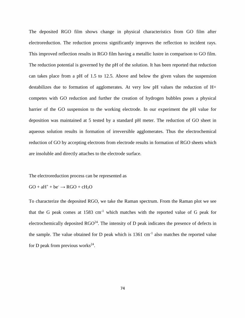
74
The deposited RGO film shows change in physical characteristics from GO film after
electroreduction. The reduction process significantly improves the reflection to incident rays.
This improved reflection results in RGO film having a metallic lustre in comparison to GO film.
The reduction potential is governed by the pH of the solution. It has been reported that reduction
can takes place from a pH of 1.5 to 12.5. Above and below the given values the suspension
destabilizes due to formation of agglomerates. At very low pH values the reduction of H+
competes with GO reduction and further the creation of hydrogen bubbles poses a physical
barrier of the GO suspension to the working electrode. In our experiment the pH value for
deposition was maintained at 5 tested by a standard pH meter. The reduction of GO sheet in
aqueous solution results in formation of irreversible agglomerates. Thus the electrochemical
reduction of GO by accepting electrons from electrode results in formation of RGO sheets which
are insoluble and directly attaches to the electrode surface.
The electroreduction process can be represented as
GO + aH+ + be- → RGO + cH2O
To characterize the deposited RGO, we take the Raman spectrum. From the Raman plot we see
that the G peak comes at 1583 cm-1 which matches with the reported value of G peak for
electrochemically deposited RGO24. The intensity of D peak indicates the presence of defects in
the sample. The value obtained for D peak which is 1361 cm-1 also matches the reported value
for D peak from previous works24.

75
Figure 9.(a) Figure 9. (b)
Figure9.(c) Figure 9. (d)
Figure 10. SEM images for RGO films for different cycles of reduction
In figure 9 the evolution of RGO film as a function of number of cycles of reduction is shown as
SEM images for 10,000X magnification. Fig 9(a) is for 3 cycles of reduction which shows onset
of inter-dispersed grains of RGO and agglomeration being deposited which are formed due to
expansion of RGO during deposition. Fig 9(b) and (c) shows the RGO film formed after 15 and
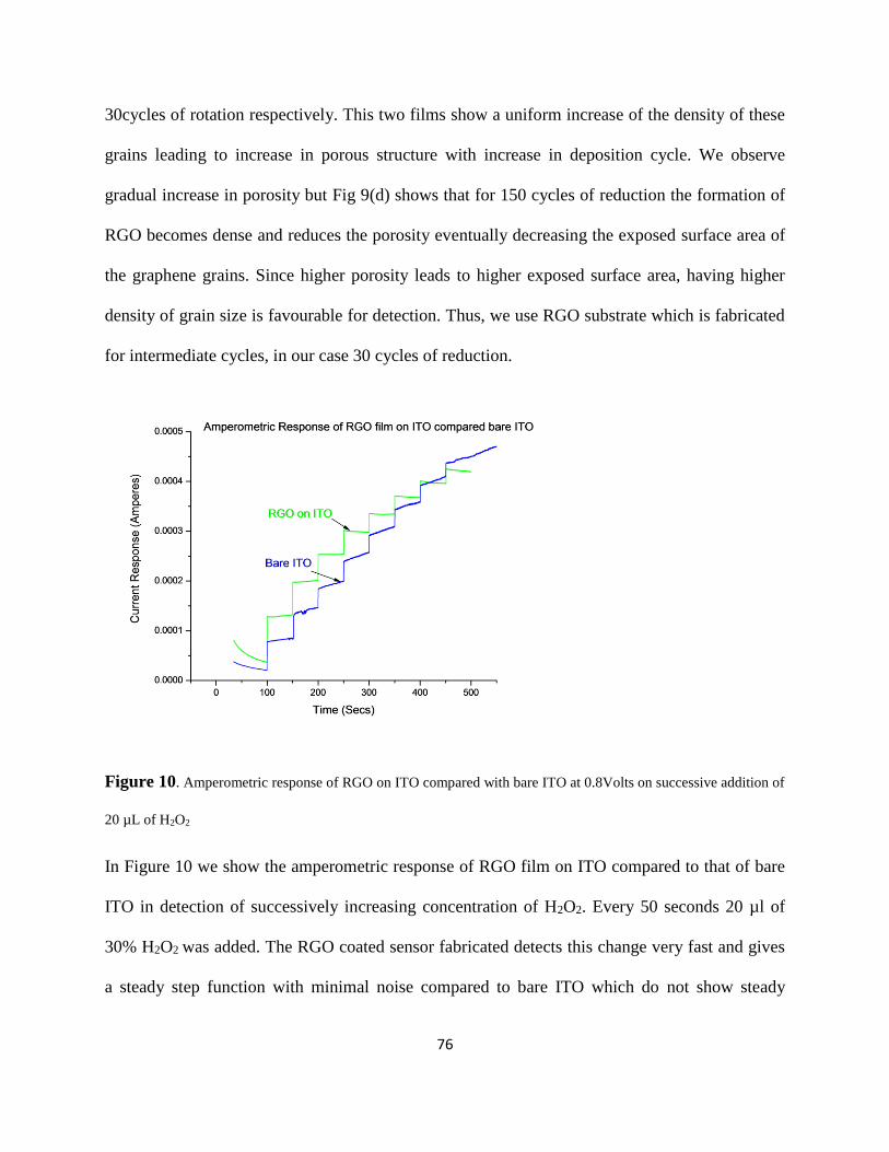
76
30cycles of rotation respectively. This two films show a uniform increase of the density of these
grains leading to increase in porous structure with increase in deposition cycle. We observe
gradual increase in porosity but Fig 9(d) shows that for 150 cycles of reduction the formation of
RGO becomes dense and reduces the porosity eventually decreasing the exposed surface area of
the graphene grains. Since higher porosity leads to higher exposed surface area, having higher
density of grain size is favourable for detection. Thus, we use RGO substrate which is fabricated
for intermediate cycles, in our case 30 cycles of reduction.
Figure 10. Amperometric response of RGO on ITO compared with bare ITO at 0.8Volts on successive addition of
20 µL of H2O2
In Figure 10 we show the amperometric response of RGO film on ITO compared to that of bare
ITO in detection of successively increasing concentration of H2O2. Every 50 seconds 20 µl of
30% H2O2 was added. The RGO coated sensor fabricated detects this change very fast and gives
a steady step function with minimal noise compared to bare ITO which do not show steady

77
current w.r.t. time. From the graph it is clear that RGO is a better sensing platform than bare ITO
as the current response of bare ITO does not stabilize which points to the fact that the current
response maybe due to other factors like conductivity of the coating. But we see that for the case
of RGO coated sensor for higher concentration the devise exhibits nonlinear performance (i.e.,
sign of saturation).
3.7 Conclusion:
Park et. al.25 have shown that the Au coated ZnO NR interface acts as a Schottky barrier which
blocks the electron transfer back from ZnO to the Glucose oxidase (GOx). This increases the
electron density at the ZnO conduction band and hence increases the efficiency of the glucose
sensor. Successful testing of glucose biosensor in our laboratory motivated us towards an
enzymeless route of detection of biomolecules. Since hydrogen peroxide is an important by
product in most enzymatic reactions we attempt to detect H2O2 in a non-enzymatic route using
electrochemically reduced graphene oxide.
References :
1) Shiping Song, Hui Xu, Chunhai Fan, International Journal of Nanomedicine 1(4), 433–440 (2006)
2) Adams DA, Brus L, Chidsey CED, et al. J Phys Chem B. 107, 6668–97 (2003).
3) U. Yogeswaran, S.M. Chen, Sensors 8, 290 (2008).
4) X.W. Sun, J.X. Wang, A. Wei, Journal of Materials Science and Technology 24, 649 (2008).
5) Z. Zhao, W. Lei, X. Zhang, B. Wang, H. Jiang, Sensors 10, 1216 (2010).
6) J. Wang. Chemical Reviews 108, 814 (2008).
7) S. Vaddiraju, D.J. Burgess, I. Tomazos, F.C. Jain, F. Papadimitrakopoulos. Journal of Diabetes Science
and Technology 4, 1540 (2010).
78
8) C.T. Campbell, J.C. Sharp, Y.X. Yao, E.M. Karp, T.L. Silbaugh. Farraday Discuss. (The Royal Society
of Chemistry) 152, 227 (2011).
9) American Diabetes Association, Clinical Diabetes 18 (2), 2000.
10) American Diabetes Association (2006). "January 2006 Diabetes Care". Diabetes Care 29
(Supplement 1): 51–580. PMID 16373931. Standards of Medical Care-Table 6 and Table 7, Correlation
between A1C level and Mean Plasma Glucose Levels on Multiple Testing over 2–3 months.
11) Giugliano D, Marfella R, Coppola L, et al. Circulation 95 (7): 1783–90 (1997).
12) Y. Liu, X. Dong and P. Chen, Chem. Soc. Rev., 41, 2283 (2012).
13) Pushpendra Kumar et al., Reviews in Advanced Sciences and Engineering 2, 1–21 (2013).
14) United States Environmental Protection Agency. Hydrazine Hazard Summary-Created in April 1992;
Revised in January 2000.
15) Y.L. Zhong, et al., Mater. Today (2014).
16) D. R. Dreyer, S. Park, C. W. Bielawski and R. S. Ruoff, Chem. Soc. Rev. 39, 228 (2010).
17) Wei Gao,Lawrence B. Alemany,Lijie CiandPulickel M. Ajayan, Nature Chemistry 1, 403 - 408
(2009)
18) Shuxian Maoa, Yumei Longa, Weifeng Lia, Yifeng Tua, Anping Deng, Biosensors and Bioelectronics
48, 258–262 (2013).
19) Nicholson, R. S.; Irving. Shain, Analytical Chemistry 36 (4): 706–723 (1964).
20) Dmitriy A. Dikin et al., Nature 448, 457-460 (2007).
21) Ganganahalli K. Ramesha and Srinivasan Sampath, J. Phys. Chem. C. 113 (19), 7985–7989 (2009)
22) Jianfeng Ping, Yixian Wang, Kai Fan, Jian Wu, Yibin Ying, Biosensors and Bioelectronics 28, 204–
209 (2011).
23) Kaiwu Chen et al., J. Mater. Chem. 22, 20968 (2012).
24) Joe Hodkiewicz, Thermo Fisher Scientific, Madison, WI, USA, Application Note: 51946A

79
25) Park, W.I., Yi, G.C., Applied Physics Letters 82, 4358-4360 (2003)

80
Chapter 4
Physical Properties of wrinkled graphene surfaces
4.1 Introduction : Graphene – Nucleobase Interactions
Graphene−nucleobase interactions is gaining importance due to its possible therapeutic
applications. Nanometer-sized graphene has emerged as a two-dimensional material with unique
chemical and electronic properties1,2. Pristine graphene has very high conductivity. It even shows
room temperature ballistic transport. It possesses excellent thermal conductivity and mechanical
strengths3,4. Due to its physical properties it can be used in electronics as well as biological
applications. It has been used in biosensors5,6, chemical sensors7, transparent conductors8, and
has many biological applications9. In our thesis we have used reduced graphene oxide as a
hydrogen peroxide sensor. Since hydrogen peroxide is the end product of interaction with many
biological enzymes, this kind of study is useful and can be extended to biosensors. Along with its
unique physical, chemical, and electronic properties, its interesting shape and size make it a
promising nanomaterial in many biological sensing. As nanographene has limited
hydrophobicity, the edges are slightly polar and the faces are highly hydrophobic10−13 it has the
capability to pass through biological membranes. This is due to the structure of biological
membranes which is a lipid bilayer membrane. Graphene−nucleobase complexes are even more
amphiphilic as the nucleobases can favorably interact with the lipid head-groups while the
graphene components would tend to be stabilized toward the central hydrophobic part of the
bilayer membrane.
These interactions together can permit the complex to pass through the cell membrane. This
property can be used in selective transport of many drugs and molecules through the lipid bilayer
membrane of the cell. The above characteristic allows graphene to act as a drug delivery vehicle,

81
which has been discussed by various groups9,14,15. Non-covalent interactions play crucial role in
molecular self-assembly and molecular recognition. The main contributions to the non-covalent
interactions come from electrostatics, hydrogen bonding, stacking, and van der Waals
interactions. Among these contributions, dispersion interaction, a component of van der Waals
interaction, acts as a major attractive interaction between nonpolar molecules. Interactions of
graphene with different hosts (many organic small molecules, nucleobases, and drugs) are also
guided by non-covalent interactions. However, dispersion interactions including π−π stacking
plays a crucial role in stabilizing such kinds of systems. The following has a little detail of such
kinds of interactions which play an important part in cell transport.
Different aromatic drugs, which are used in cancer therapy, can be loaded on the graphene sheet
through π−π stacking for intracellular drug delivery. A very important characteristic of graphene
sheet is its high surface area, where a maximum number of atoms can get exposed to the surface,
thereby making it a very important therapeutic agent for drug delivery.19 Since graphene is a two
dimensional sheet the surface atoms are readily available for binding. To understand the
interaction of graphene sheet with different biomolecules, it is important to understand the
conductivity of the graphene sheet which gives an insight into the binding property of the
graphene sheet.
All of the above studies assume perfectly planar graphene sheets and mostly of infinite
dimensions in X and Y directions.
However, it is well-known that two-dimensional crystals are never stable16,17 and have a
tendency to curl toward the edges.18,19 The conductivity property of graphene sheets on curling
has been studied by us and very interesting results have been obtained which will be discussed
below. Even pristine graphene contains many topological defects. Many reports by different

82
groups confirmed that bending in the graphene can be due to topological lattice defects,
impurities, tensions, etc13,20,21.
We used scotch tape peeling of HOPG substrate for isolating freestanding graphene
sheets dislodged from the underlying sheets.
In our experiment, we have used freshly cleaved highly oriented pyrolytic graphite
(HOPG). Using scotch tape, we were able to peel off top few layers exposing fresh graphene
ribbons with various kind of edges. The peeling process dislocates the exposed layers laterally
and vertically. Commercial AFM (NT-MDT, Russia) was used for our investigation. Cantilevers
used were platinum coated (CSG 10/Pt, NT-MDT) with a radius of curvature of the tip 35 nm
and the cantilever elastic constant 0.1 N/m. For imaging in the contact mode the normal force
between the surface and the tip was kept around 25 nN (constant force mode). The sample was
biased with 10 to 15 mV for measuring the local conductance (spreading resistance imaging) of
the sample surface with the conducting tip. By measuring the tip−sample contact conductance
(resistance) during the scanning process, we estimate the local conductance of the sample
surface. All of the measurements were conducted at room temperature and ambient conditions.
For topographic images, we have only subtracted the linear line fit along the scan direction from
the scanned images and presented without any further averaging. For the conductance map also,
we show only the raw results without any signal processing.
4.2 Results and Discussions :
We observed formation of ripple/wrinkles at the edges of the graphene sheet dislodged
from the underlying HOPG substrate as indicated by arrows by using AFM in conductivity mode
(Figure 2). The ripples at the graphene edges are smaller in wavelength (less than 50 nm) than
the ripples formed on the interior surface of the HOPG marked by regions A and B (around 300

83
nm). The separation between the layers A and B is about 0.8 nm. It is interesting to note that
since the edges of the graphene sheets, which may be more loosely bound than the top interior
surface, the ripples formed at the edges are of shorter wavelength than that of ripples formed on
the top interior graphene sheet. This gives an indication that the free standing graphene sheet
may have much smaller wavelength ripples and as the thickness of graphene sheet increases (few
layers bound together), the wavelength will increase as discussed by Bao et al.22
Figure 2. Top: 3-dimensional and bottom: 2-dimensional AFM image showing ripple/wrinkles formation
at the edge of the graphene sheet dislodged from the underlying highly oriented pyrolytic graphite
(HOPG). The arrows indicate smaller wavelength ripples at the edges. Regions marked A and B are the
large wavelength ripples.
This appearance of curvature is presumably due to adoption of partial sp3 character by some of
the carbon atoms present toward the edges, owing to its unusual edge property. In order to verify
sp3 characteristic of graphene upon bending, we have carried out local conductivity mapping

84
along with topography using conducting tip atomic force microscopy (CT-AFM12,23) around a
folded region of graphene bound to underlying HOPG, which acts as a substrate.
Figure 3. (a) AFM topographical map and (b) local conductivity map around a folded region of graphene.
The bright region corresponds to higher current indicating higher conducting regions and the darker
regions are the low conducting regions as shown in grey scale bar. The dark streak-like regions at the
bend shown by arrow are the low conducting regions indicating formation of sp3 characteristic upon
bending.
In Figure 3, we show local conductivity map around a folded region of graphene along with the
topographical map. The bright region corresponds to higher current, indicating higher conducting
regions and the darker regions are the low conducting regions as shown in grey bar scale. We

85
clearly observe that the peeled graphene portion are brighter indicating higher conducting
property as discussed earlier.12,23 Interestingly, we also clearly see dark streak-like regions at all
of the bends (shown by arrows) and this indicates that the conductivity is low due to formation of
sp3 characteristics upon bending. For the sp3 characteristic (3D), the electrons will be localized
unlike the sp2 characteristics, which allows the electrons to hop around the 2D graphene sheet.
4.3 Conclusion
From our experimental work we can conclude that free graphene sheet will always form
wrinkle/ripple as a stable form. The wrinkle arise due to next near neighbour interaction and
simulation based on dispersion corrected density functional theory (DFT-D) approach plays a
significant role in making a planar graphene sheet a non-planar. At the bend the conductivity
showing low values indicates sp3 characteristic of graphene upon bending.
The future scope and conclusion of this experiment has been detailed in the last chapter.
References
(1) Hernandez Rosas, J. J.; Ramírez Gutierrez, R. E.; Escobedo-Morales, A.; Chigo Anota, E. J. Mol.
Model. , 17, 1133−1139 (2011)
(2) Novoselov, K. S.; McCann, E.; Morozov, S. V.; Falko, V. I.; Katsnelson, M. I.; Zeitler, U.; Jiang, D.;
Schedin, F.; Geim, A. K. Nat. Phys., 2, 177−180 (2006)
(3) Balandin, A. A; Ghosh, S.; Bao, W. Z.; Calizo, I.; Teweldebrhan, D.; Miao, F.; Lau, C. N. Nano Lett. ,
8, 902−907 (2008)
(4) Lee, C.; Wei, X. D.; Kysar, J. W.; Hone, J. Science, 321, 385−388 (2008)
75
(5) Yang, W.; Ratinac, K. R.; Ringer, S. P.; Thordarson, P.; Gooding, J. J.; Braet, F. Angew. Chem., Int.
Ed. , 49, 2114−2138 (2010)
(6) Shao, Y.; Wang, J.; Wu, H.; Liu, J.; Aksay, I. A.; Lin, Y. Electroanalysis, 22, 1027−1036 (2010)

86
(7) Fowler, J. D.; Allen, M. J.; Tung, V. C.; Yang, Y.; Kaner, R. B.; Weiller, B. H. ACS Nano , 3,
301−306 (2009)
(8) Wassei, J. K.; Kaner, R. B. Mater. Today, 13, 52−59 (2010)
(9) Sun, X.; Liu, Z.; Welsher, K.; Robinson, J. T.; Goodwin, A.; Zaric, S.; Dai, H. Nano Res. , 1, 203−212
(2008)
(10) Yang, H.; Fung, S. Y.; Pritzker, M.; Chen, P. PLoS One , 2, e1325 (2007)
(11) Panigrahi, S.; Bhattacharya, A.; Bandyopadhyay, D.; Grabowski, S. J.; Bhattacharyya, D.; Banerjee,
S. J. Phys. Chem. C., 115, 14819−14826 (2011)
(12) Banerjee, S.; Sardar, M.; Gayathri, N.; Tyagi, A. K.; Raj, B. Phys. Rev. B, 72, 075418 (2005)
(13) Banerjee, S.; Bhattacharyya, D. Comput. Mater. Sci., 44, 41−45 (2008)
(14) Liu, Z.; Robinson, J. T.; Sun, X.; Dai, H. J. Am. Chem. Soc., 130, 10876−10877 (2008)
(15) Yang, K.; Zhang, S.; Zhang, G.; Sun, X.; Lee, S. T.; Liu, Z. Nanolett., 10, 3318−3323 (2010)
(16) Hohenberg, P. C. Phys. Rev., 158, 383−386 (1967)
(17) Mermin, N. D.; Wagner, H. Phys. Rev. Lett., 17, 1133−1136 (1966)
(18) Pereira, V. M.; Castro Neto, A. H.; Liang, H. Y.; Mahadevan, L. Phys. Rev. Lett., 105, 156603
(2010)
76
(19) Gil, A. J.; Adhikari, S.; Scarpa, F.; Bonet, J. J. Phys.: Condens. Matter, 22, 145302 (2010)
(20) Thompson-Flagg, R. C.; Moura, M. J. B.; Marder, M. EPL (Europhys. Lett.), 85, 46002 (2009)
(21) Guinea, F.; Horovitz, B.; Le Doussal, P. Solid State Commun., 149, 1140−1143 (2009)
(22) Bao, W.; Miao, F.; Chen, Z.; Zhang, H.; Jang, W.; Dames, C.; Lau, C. N. Nat. Nanotechnol. , 4,
562−566 (2009)
(23) Banerjee, S.; Sardar, M.; Gayathri, N.; Tyagi, A. K.; Raj, B. Appl. Phys. Lett., 88, 062111 (2006)
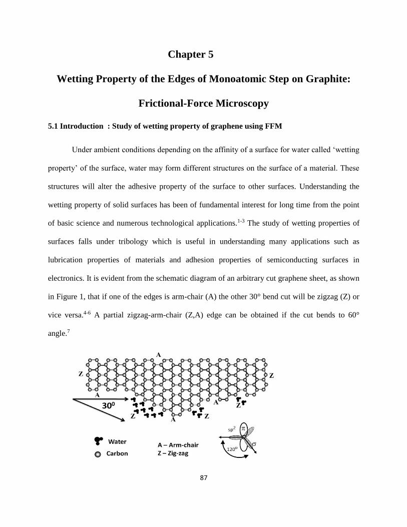
87
Chapter 5
Wetting Property of the Edges of Monoatomic Step on Graphite:
Frictional-Force Microscopy
5.1 Introduction : Study of wetting property of graphene using FFM
Under ambient conditions depending on the affinity of a surface for water called ‘wetting
property’ of the surface, water may form different structures on the surface of a material. These
structures will alter the adhesive property of the surface to other surfaces. Understanding the
wetting property of solid surfaces has been of fundamental interest for long time from the point
of basic science and numerous technological applications.1-3 The study of wetting properties of
surfaces falls under tribology which is useful in understanding many applications such as
lubrication properties of materials and adhesion properties of semiconducting surfaces in
electronics. It is evident from the schematic diagram of an arbitrary cut graphene sheet, as shown
in Figure 1, that if one of the edges is arm-chair (A) the other 30° bend cut will be zigzag (Z) or
vice versa.4-6 A partial zigzag-arm-chair (Z,A) edge can be obtained if the cut bends to 60°
angle.7

88
Figure 1. Schematic diagram of an arbitrary cut graphene.
Intuitively, one may expect similar electron accumulation at both edges. However, it was
reported earlier that there exist distinct electronic properties at these edges.8-21 The properties of
the two kinds of edges of graphene are elaborated below.
Graphene nanoribbons will have structural variations at its edges leading to different
electronic states at different edges called the edge states. 2D graphene is a zero gap
semiconductor but to extend the application of graphene to electronics an energy gap has to be
introduced which enables the ON-OFF state which are the basic electrical logic state. When
graphene is etched preferentially in a particular direction or patterned we get two types of edges
of graphene, the zig-zag and armchair edge.
Zig-zag type nanoribbons exhibit metallic properties whereas armchair nanoribbon are
semiconducting or metallic depending on its chirality.
Structural Dynamics: The width of armchair graphene nanoribbon is determined by
counting the number of dimmers across the chain. Similarly, the width of zig-zag graphene
nanoribbon is determined by the number of zig-zag chains across the ribbons. Perpendicular to
the direction of the measurement of width of the graphene nanoribbon, they repeat their
geometric structure.
In pristine condition, the graphene edges are unsaturated. The final structure of graphene
edge depends on the type of atom which terminates the edges. For armchair edge there is no
reconstruction of the edges and the graphene armchair edge remains planar. However for zig-zag
edges planarity is maintained for H terminated edges. In the theoretical model developed by our
collaborators, zig-zag edges were considered to be H-terminated. All armchair ribbons are
89
semiconductors with a energy gap which decreases with increasing width of the nanoribbon. The
armchair nanoribbons are hydrogen passivated which makes carbon atom at the edges have
different bond length than carbon atom at the centre with the latter having a longer bond length.
Zig-zag edges have doubly degenerate flat edge bands at Fermi level.
5.2 Experimental Details
Our experimental studies using frictional force microscopy on a pyrolytic graphite
surface also indicates differential interaction between water and the two edges of graphene. We
have used freshly cleaved highly oriented pyrolytic graphite (HOPG) for the present
investigation. We obtained terraces with single monolayer (monatomic) step edges by simply
peeling off the surface layers using scotch tape. Commercial atomic force microscope (AFM)
(NT-MDT, Russia) was used for the present investigation. Gold-coated cantilevers with Si3N4
tip CSG 10, NT-MDT with a radius of curvature of the tip ∼350 Å and the cantilever elastic
constant 0.1 N/m is used for this experiment without any further functionalization. Experiments
carried out by different groups provide indirect evidence about the hydrophilic nature of the
AFM tip. The works carried by different groups22,23 have shown that water bridge forms between
the as-procured commercial AFM tip (nonfunctionalized) and the hydrophilic substrate,
indicating hydrophilic nature of the AFM tip. If the tip is hydrophobic, then the tip will not
interact with water and hence it would be impossible to distinguish the wetting from the
nonwetting edges. For imaging in the contact mode, the normal force between the surface and
the tip was kept around 25 nN in a constant force mode. The AFM and the frictional force
microscopy. (FFM) measurements were carried out in contact mode.
All measurements were performed at room temperature (26 °C) at different relative
humidity (RH). The scan size for all of the samples was 2 μm in length on each side. In the

90
frictional force microscopic technique, one can simultaneously measure both the topography and
the frictional property by recording the current signals Iver and Itor, where Iver gives the magnitude
of normal bending of the cantilever (topography) and Itor gives the magnitude of torsional or
lateral bending of the cantilever (friction). For more details on FFM, please see ref 24.
Figure 2. A 3-dimensional topographic image of a monolayer step is represented in (a). Parts (b) and (c)
show the FFM images of the same region with scan direction right to left and left to right, respectively.
The Figure (d) shows a blown up region.
In Figure 2a, we show a 3-dimensional topographic image of a monatomic step and in
Figure 2b,c we show the FFM image of the same region with scan direction right to left (R to L)
and left to right (L to R) respectively. We clearly see the contrast inversion of the FFM images
for the scan in forward and backward directions (see ref 24 for detail). In Figure 2d, we show a

91
blown up region marked by a box, which clearly shows distinctly bright and dark regions along
the step. The bright region corresponds to higher frictional (higher Itor i.e., higher lateral bending
of the cantilever) value and the lighter region along the cut indicates low friction value. This
clearly indicates the existence of two distinct types of frictional property along the cut. It should
be pointed out here that the graphite surface is hydrophobic and earlier experiments suggest that
upon increasing relative humidity the surface would not get covered with water.25-27
Figure 3. Schematic diagram showing torsional bending of the cantilever during a line scan along the
forward (left to right) directions, in different environmental conditions: (i) when the step edge contain no
water (ii) when the step edge contains small water droplets (iii) when the step edge contains larger water
droplets. The right-hand figure shows schematic histogram plot of the torsional bending of the cantilever
proportional to the current Itor.
In Figure 3, we schematically show the data analysis scheme adopted in this
investigation. In the left panel of Figure 3, we show the amount of torsional bending of the

92
cantilever during a line scan perpendicular to the cut along the forward (left to right-downward
scan, i.e., going down the step) directions (shown by an arrow) having angle (θ’s). The torsional
angle (θ) is the measure of frictional force between the tip and the sample surface. We have
shown, in Figure 3, three situations “i” to “iii” of torsional bending of the AFM tip. In situation
“i”, when the tip is moving on top of the graphite layer (terrace) the torsional bending is the least.
When the tip arrives at the edge of the monatomic graphite layer, the torsional bending angle (θi)
increases and for situation “ii” with the edge containing water droplet the torsional bending θii is
larger than θi, this is because the water droplet acts as a glue22,23 and tries to hold back the tip as
the tip moves toward forward direction. For a larger water droplet (situation “iii”) the torsional
bending angle will be further increased to θiii where now θiii > θii, this is again because the larger
water droplet will have a much larger restoring or holding back force on the tip than the smaller
water droplet. In Figure 3 on the right panel we have schematically shown a histogram plot of the
torsional bending of the cantilever proportional to the current, indicating Itor, proportional to θ.
We would like to mention that throughout our experiment for all of the scans the position of the
laser beam on the cantilever was kept on the same spot and the scan speeds were also maintained
the same. This is very important since we know that variation of the position of the laser beam
on the cantilever and its speed affects the measure of bending of the cantilever, hence in turn will
affect its frictional property also. In Figure 3, we show (schematically in the histogram plot) that
apart from the main peak around zero torsional bending, which arises due to the top surface of
the graphite (the terraces), there exist a second peak appearing as a shoulder to the main peak and
one more third peak far away from the main central peak. These two extra peaks will be very
small in magnitude compared to the main central peak because the histogram height will be
proportional to the amount of area having that particular frictional property.

93
The area along the step (a curved single line in the case of monatomic graphite layer) will
be very small compared to the total surface area scan of the sample. The shoulder and the peak
appearing at larger torsional bending angle are due to the monatomic steps. If there are two
different frictional properties along the step, then we should also see two distinct peaks apart
from the main peak. Two different types of steps along the edges have been shown by an STM
images by Kobayashi et. al.4,7 As the size of the water droplet increases the secondary side peak
should shift to higher torsional bending value because larger water droplet will cause larger
pulling back force as shown schematically in Figure 3, whereas, edges where water does not
condenses the secondary peak should not shift. Most interestingly when the tip is scanned in the
reverse direction (from the right to left i.e., going up the step) the step height acts as a barrier,
which does not allow water to be pulled by the tip. Thus the frictional scans have very low
sensitivity to feel the water droplets along the edge in the reverse scan direction (R to L), which
we have observed from our experimental measurement as shown in Figure 4. Hence, for our
experimental investigation to study the wetting property of graphene edge, we have only
considered the left to right forward scan. The peak “ii” in Figure 3 is for edges with water droplet
and with the increase in RH (i.e., water droplet size) this peak moves to position “iii”. The peak
“i” does not move with increase in RH in those parts of the edges where water does not
condense.

94
Figure 4. Experimental histogram plots of torsional bending of the cantilever as a function of increase of
relative humidity (RH = 60, 65, and 70%) for downward and upward scan as shown in (a). In part (b), the
deconvoluted lines are also shown (see text for details).
In Figure 4a we have presented the experimental histogram plot of torsional bending of
the cantilever as a function of increase in relative humidity (RH = 60, 65, and 70%) of a
monatomic step edge on highly oriented pyrolytic graphite (HOPG) using FFM. The histogram
was obtained after flattening the data, this is done to reduce the noise in the histogram plots,
which arises due to vibration of the samples and other disturbances due to electrical and thermal
noise. The flattening of the data causes the main major peaks due to terraces to be around zero
lateral bending value for both the left to right (L to R) and right to left (R to L) scans and this can
be considered as the background. Hence the absolute frictional value of the terraces is considered
as background, as we are only interested in obtaining the frictional properties of the edges, not in
absolute scale. The error in the lateral bending can be obtained from the fluctuation of the lateral

95
signal when scanning over a homogeneous area (in our case, in the terraces) and we found it to
be around 1.2 pA (full width at half-maximum), which is 1.2 unit in the x-axis of the histogram
plot, almost the size of the symbols used in the plot. We clearly see a major peak corresponding
to the surface (terraces) and two side peaks due to the edges during forward scan (L to R). The
distant peak corresponding to large torsional bending (friction) has been attributed to the wet
edges containing water and the side shoulder peak to the nonwetting edges.We also see that the
peaks associated to the wet edges significantly shift toward higher torsional bending value,
clearly indicating an increase in the water content as a function of increase in the RH, as
discussed above. The two side peaks were analyzed by deconvoluting the peaks as shown in
Figure 4b and we distinctly observe that as the percentage of RH increases the peak positions
marked by arrow shift toward higher torsional bending values, whereas the shoulder peak does
not show any systematic increase in the torsional bending value. In Figure 4a, we also show the
histogram plot of the reverse scan (upward scan) and we clearly see that the histogram is not
sensitive to the wetting property of the monatomic graphite edge.
Thus, from our experimental results, we find presence of two different frictional properties along
the edges of a graphene sheet.
5.3 Conclusions:
In this investigation, we have observed presence of two different frictional properties along
monatomic step edges on graphite using Frictional Force Microscopy. The two different
frictional properties can be attributed to two different types of edges of this layer, namely zigzag
(or trans) edge and arm-chair (or cis) edge. These differential frictional properties are also seen
to be dependent on the relative humidity of the experimental conditions—the frictional property
of one of the edge type depends on humidity while that of the other edge type remains constant.

96
Thus, the two edges appear to have different modes of binding to water molecules. The
theoretical calculations (carried out by our collaborator) enabled us to find out the mechanism of
interaction of water with the two different types of edges of the graphene. The interaction
energies calculated suggests that the zigzag edge of graphene has a stronger binding capacity
with the water molecule than the arm-chair edges. Thus, we could conclude that the zig-zag
edges are hydrophilic (collects water at this edge type) and armchair edges are hydrohopic (water
do not collect at this edge type).
References
(1) Herminghaus, S.; Brinkmann, M.; alf Seemann, R. Annu. Rev. Mater. Res. 2008, 38, 101–121.
(2) Bonn, D.; Eggers, J.; Indekeu, J.; Meunier, J.; Rolley, E. Rev. Mod. Phys. 2009, 81, 739–805.
(3) Sarkar, S.; Patra, S.; Gayathri, N.; Banerjee, S. Appl. Phys. Lett. 2010, 96, 063112.
(4) Kobayashi, Y.; Fukui, K.; Enoki, T.; Kusakabe, K.; Kaburagi, Y. Phys. Rev. B 2005, 71, 193406.
(5) Banerjee, S.; Sardar, M.; Gayathri, N.; Tyagi, A. K.; Raj, B. Phys. Rev. B 2005, 72, 075418.
(6) Banerjee, S.; Sardar, M.; Gayathri, N.; Tyagi, A. K.; Raj, B. Appl. Phys. Lett. 2006, 88, 062111.
(7) Kobayashi, Y.; Fukui, K.; Enoki, T.; Kusakabe, K. Phys. Rev. B 2006, 73, 125415.
(8) Fujita, M.; Wakabayashi, K.; Nakada, K.; Kusakabe, K. J. Phys. Soc. Jpn. 1996, 65, 1920–1923.
(9) Nakada, K.; Fujita, M.; Dresselhaus, G.; Dresselhaus, M. S. Phys. Rev. B 1996, 54, 17954.
(10) Wakabayashi, K.; Fujita, M.; Ajiki, H.; Sigrist, M. Phys. Rev. B 1999, 59, 8271–8282.
(11) Stein, S. E.; Brown, R. L. J. Am. Chem. Soc. 1987, 109, 3721–3729.
(12) Hosoya, H.; Gao, Y. D.; Nakada, K.; Ohuchi, M. In New Functionality Materials; Tsuruta, C. T.,
Doyama, M., Sena, M., Eds; Elsevier: New York, 1993, 27.
(13) Tanaka, K.; Yamashita, S.; Yamabe, H.; Yamabe, T. Synth. Met. 1987, 17, 143–148.
(14) Fujita, M.; Yoshida, M.; Nakada, K. Fullerene Sci. Technol. 1996, 4, 565.

97
(15) Ryu, S.; Hatsugai, Y. Physica E (Amsterdam) 2004, 22, 679.
(16) Wakabayashi, K. Phys. Rev. B 2001, 64, 125428.
(17) Elstner, M.; Porezag, D.; Jungnickel, G.; Elsner, J.; Haugk, M.; Frauenheim, T.; Suhai, S.; Seifert, G.
Phys. Rev. B 1998, 58, 7260–7268.
(18) Kobayashi, Y.; Fukui, K. I.; Enoki, T.; Kusakabe, K.; Kaburagi, Y. Phys. Rev. B 2005, 71, 193406.
(19) Dedkov, Y. S.; Shikin, A. M.; Adamchuk, V. K.; Molodtsov, S. L.; Laubschat, C.; Bauer, A.; Kaindl,
G. Phys. Rev. B 2001, 64, 035405.
(20) Nimi, Y.; Matsui, T.; Kambara, H.; Tagami, K.; Tsukada, M.; Fukuyama, H. Appl. Surf. Sci. 2005,
241, 43.
(21) Geim, A. K.; Novoselov, K. S. Nat. Mater. 2007, 6, 183–191.
(22) Jinesh, K. B.; Frenken, J. W. M. Phy. Rev. Lett. 2006, 96, 166103.
(23) Wei, Z.; Zhao, Y.-P. J. Phys. D: Appl. Phys. 2007, 40, 4368.
(24) Banerjee, S.; Gayathri, N.; Shannigrahi, S. R.; Dash, S.; Tyagi, A. K.; Raj, B. J. Phys. D: Appl. Phys.
2007, 40, 2539.
(25) Yang, H.; Fung, S. Y.; Pritzker, M.; Chen, P. PLoS One 2007, 2, e1325.
(26) Biswas, S.; Drzal, L. T. Nano Lett. 2009, 9, 167–172.
(27) Leenaerts, O.; Partoens, B.; Peeters, F. M. Phys. Rev. B 2009, 79, 235440.

98
Chapter 6
Identifying bacterial fragments using Ultrasonic-AFM
6.1 Introduction : Ultrasonic AFM imaging of bacterial cells
Different cells have different cellular dimensions and different cell wall thickness
depending on which part of the body they are units of. For instance a muscle cell and a bone cell
will have completely different morphology and thus, completely different elasticity which is
tuned to the functionality of the organ of which the cell is a constituent. In fact depending on the
different load bearing needs of different parts of the body, muscle cells have different
dimensions and thus, different elasticity and load bearing capacity. Elasticity mapping of cells
can also be used in diagnostics. Certain strains of E.Coli bacteria release a toxin which deform
the RBC in blood changing the elasticity of the cell. Thus, mapping RBC elasticity the extent of
damage by invading bacteria can be gauged and corrective drugs employed. There has already
been work done on differentiation of cancer cells from normal functional cells in the body by
mapping elasticity of newer and softer cancer cells against harder functional cells. This method
makes cancer diagnosis possible way before malignancy sets in. Fate mapping of an embryo has
been done through optical analysis. However, fate mapping of embryo can be done by elasticity
mapping and relating parts which have a similar mechanical property evolution.
There has been a lot of work done on imaging of bacterial cells using the atomic force
microscope [1]. Also there has been a lot of work done on the elasticity of cells and its relation to
living system of an organism [2]. There has been work done previously on imaging human cells
which are optically identical i.e., all cells look alike under an optical microscope. However,
when the elasticity of these cells was mapped it was seen that certain cells are much softer than

99
other cells [3]. These cells are the cancer cells. Hence, it is possible to diagnose cancer cells
much before malignancy stage. Work has also been done on the elasticity of red blood cells
during malaria when it becomes much harder than it normally is [4] and thus offers resistance to
flow in the blood vessels which leads to the shooting temperature. All this information can be
provided by the ultrasonic AFM (UFM) also. It can also give the elasticity mapping of the whole
surface of the bacteria and the substrates. This helps to identify areas in the bacterial surface
which have the same elasticity and thus surfaces which fragmented at about the same time. It
also helps to distinguish between the hard surface of the immobilizing substrate and the soft
surface of the bacteria. Thus, combining both the technique of the AFM and UFM it is possible
to know both the morphology and elasticity of the bacterial surface. This whole chapter
highlights that UFM is a very powerful technique available to scientists for imaging cells and
qualitatively determining their surface elasticity. This technique helps to qualitatively look at cell
wall elasticity.
In response to nutrient depletion and other hazardous factors, a bacterial cell undergoes
lysis or cell death. The question that has never been addressed before is that what the structural
modification of the cell is during this process. Structural modifications can be studied using
UFM during cell growth and death process. The structural modification also point to the
metabolic changes during cell death and hence, is an important factor in understanding cell
death. Certain bacterial strains are known to survive in very extreme conditions. Bacterial cells
due to exposure to these extreme conditions get fragmented. In certain bacteria these fragments
when kept in a suitable nutrient medium they regenerate into live cells [5]. However the extent of
injury determines whether the process is reversible or not. Hence studying the fragmentation
100
pattern would give important information regarding the cell’s regenerative capability. This is the
reason behind studying the bacterial cells [6] by using UFM to show its potential.
6.2 Experimental Section:
These bacterial cells were immobilized on anodized Ti substrate to study the bactericidal
activity of the substrate [7]. The immobilized bacterial cells were stored in ambient surroundings
for a long period. Pseudomonas sp is used as a test bacteria to gauge the potency of UFM
technique in determining the elasticity of the bacterial surface. The objective behind selecting
these bacteria is that it is found to recover after fragmentation and severe injury. There are two
techniques of the AFM, the atomic force acoustic microscope (AFAM) and the ultrasonic force
microscope (UFM) where in the former the sample and in the latter the cantilever tip is vibrated
at ultrasonic frequencies. Both these techniques probe elasticity of sample at nanoscale [8] and
hence are important techniques to estimate the elasticity of the bacteria at nanoscale. Some of the
modified techniques used to obtain the local elastic properties are force modulation microscopy
[9], force versus distance curve [10], nanoindentation [11], scanning micro-deformation
microscopy [12]. Banerjee et al.[8] have compared the UAFM and AFAM techniques in one of
their paper and showed both techniques yield similar results. For the measurements we used
boron doped silicon cantilever from NT-MDT(Model NSG10) with elastic constant kc ∼
20Nm−1, radius of curvature of the tip∼10 nm, tip height 10–15μm, aspect ratio 3 : 1, cone angle
~ 22° and free resonance frequency of fo ∼ 320 kHz. For imaging we have used typically a
normal force FN ∼ 1.5μN. All the measurements were performed in ambient atmosphere to
monitor sample fragmentation from natural causes only. In this particular technique we have
used UFM to image the bacteria as we only need to see the elastic properties of the bacteria in a
semi-quantitative approach.

101
6.3 Results and discussions:
In fig. 2 we obtain AFM images of isolated bacteria which is rod like in shape (fig. 2(a))
and clusters of the same bacteria (fig. 2(b)). From the clusters of the bacteria (fig 2(b)) we see
certain features appearing on the bacterial surface. However, the bacterial fragments have not
disintegrated as a whole. Fragmentation lines are appearing on the bacterial surface.
Figure 2: Topographic images obtained from AFM of (a) isolated bacteria and (b) clusters of bacteria.
In fig. 3 topographic images of the bacteria has been taken after a period of one year of
storage of the bacteria. This period is a long time for allowing the bacteria to die and fragment.
We observe topographic image of the fragments which appear as nodules on the surface.
However, it is not possible to say confirmatively whether it is a dust on the substrate or bacteria.
Thus to distinguish this we have to carry out elastic mapping of the surface.

102
Figure 3: Topographical images of bacterial cells observe after about more than a year. We see distinct nodules
appearing on the surface of the bacterial cell.
To clear this ambiguity we have imaged this cell in the UFM mode. The result from the
UFM technique imaging is given in fig 4. Fig 4(a) & (b) give 2D and 3D topographic image of
the bacterial surface in conjugation with the substrate on which it is immobilized. In here the
region marked as X appears as the bacterial fragment. However, in fig 4(c) & (d) the frequency
of vibration has been selected above and below the resonance frequency for which we obtain
contrast inversion for the bacterial fragments and opposite contrast inversion for the region X.
Thus, we can conclude this region X is not part of the bacterial surface.

103
Figure 4: (a) 2D and (b) 3D topographical image of fragmented bacteria but note the regions marked as X in figure it
appears as part of bacterial fragment. Images obtained using UAFM technique for the frequency (c) higher and (d)
lower than the contact resonance frequency. The region marked as X is the harder region and not fragment of the
bacteria (see text for more details).
6.4 Conclusion :
Thus, the UFM technique helps to distinguish between bacterial and substrate fragments
leading to correct information about fragmentation of bacteria. This technique can be further
extended to other biological cell systems. We can also use this techniques in medical diagnostics.
References :
[1] Judy Gopal, R.P.George, P.Muraleedharan, S.Kalavathi, S.Banerjee, H.S.Khatak, Photocatalytic
inhibition of microbial fouling by anodized Ti6Al4V alloy, Journal of Material Science, 42, (2007), 5152-
5158

104
[2] Daniel J. Müller, Yves F. Dufrêne, Atomic force microscopy as a multifunctional molecular toolbox
in nanobiotechnology, Nature Nanotechnology 3, (2008), 261-269
[3] S. E. Cross, Y. S. Jin, J. Y. Rao, J. K. Gimzewski, Nanomechanical analysis of cells from cancer
patients, Nature Nanotech. 2, (2007), 780–783.
[4] S. Majid Hosseini, James J. Feng, How Malaria Parasites Reduce the Deformability of Infected Red
Blood Cells, Biophys J., 103, (2012), 1–10
[5] Roger Dabbah, W.A. Moats, J.F. Mattick, Factors Affecting Resistance to Heat and Recovery of Heat-
Injured Bacteria, Journal of Dairy Science, 52, (1969) 608-614
[6] Prachi Tripathi, Audrey Beaussart, Guillaume Andre, Thomas Rolain, Sarah Lebeer, Jos
Vanderleyden, Pascal Hols, Yves F. Dufrêne, Towards a nanoscale view of lactic acid bacteria, Micron,
43, (2012) 1323–1330
[7] S. Banerjee, J. Gopal, P. Muraleedharan, A. K. Tyagi, B. Raj, Physics and chemistry of photocatalytic
titanium dioxide: Visualization of bactericidal activity using atomic force microscopy, Current Science,
90, (2006), 1378-1383.
[8] S. Banerjee, N. Gayathri, S. Dash, A. K. Tyagi, B. Raj, A comparative study of contact resonance
imaging using atomic force microscopy, Appl. Phys. Letts. 86, (2005), 211913-211916.
[9] P. Maivald, H. J. Butt, S. A. C. Gould, C. B. Prater, B. Drake, J. A. Gurley, V. B. Elings, P. K.
Hansma, Using force modulation to image surface elasticities with the atomic force microscope,
Nanotechnology, 2, (1991), 103-106.
[10] M. Heuberger, G. Dietler, L. Schlapbach, Mapping the local Young's modulus by analysis of the
elastic deformations occurring in atomic force microscopy, Nanotechnology, 6, (1995), 12-23
[11] Joyce, A. Stephen , J. E. Houston, A new force sensor incorporating force‐feedback control for
interfacial force microscopy, Review of Scientific Instruments, 62, (1991), 710-715.
[12] P. Vairac and B. Cretin, Scanning microdeformation microscopy in reflection mode, Applied Physics
Letters, 68, (1996), 461-463

105
[13] S. Banerjee, N. Gayathri, S. R. Shannigrahi, S. Dash, A. K. Tyagi and B. Raj, Imaging distribution
of local stiffness over surfaces using atomic force acoustic microscopy, J. Phys. D: Appl. Phys., 40,
(2007), 2539.
[14] S. Banerjee, N. Gayathri, S. Dash, A. K. Tyagi, B. Raj, Imaging elastic property of surfaces at
nanoscale using atomic force microscope, Applied Surface Science, 256, (2009), 503.

106
Chapter 7
Conclusion and future scope
In conclusion, we have studied the wetting and conductivity property of nanographene
using HOPG. This kind of study demonstrates for future researchers the powerful scope of the
AFM in detecting phenomenon operating at nanoscale. Most of the published work on graphene
is based on theoretical modelling. We provide a fresh perspective to this work by investigating
nano-graphene experimentally and then comparing the results with theoretical work done by our
collaborators. For wetting study we arrive at the conclusion that we have observed presence of
two different frictional properties along monoatomic step edges on graphite using Frictional
Force Microscopy. The two different frictional properties can be attributed to two different types
of edges of this layer, namely zigzag (or trans) edge and arm-chair (or cis) edge. These
differential frictional properties are also seen to be dependent on the relative humidity of the
experimental conditions—the frictional property of one of the edges depends on humidity while
that of the other edge remains constant. Thus, the two edges appear to have different modes of
binding to water molecules. Theoretical calculations reveals that the zig-zag edges will be
hydrophilic and arm-chair edges will be hydrophobic, and hence the experimental result could be
attributed to these two edges. In our subsequent work on conductivity of nanographene sheets we
conclude ripple formation is the inherent nature of the larger graphene sheet, which provides
structural stability to graphene sheets and is associated with the unique electronic properties of
the carbons at the bends. Interaction of graphene with the nucleobases proved that electrostatic
interactions are not the major driving forces for stabilizing such systems and the greatest
contributions for the binding energy often come from the dispersion interaction, which is

107
isotropic in nature. Future studies on graphene sheet maybe done for study of strain engineering
of graphene.
There is a lot of future scope in the study of systems such as a above through AFM. In
particular it is of interest to study the electronic properties of various GICs (Graphite Intercalated
Systems) by conductivity mapping using the AFM. These systems are specially important as they
are a precursor for production of single graphene sheets. This method would be scalable and
cheap. The most recent adaptation of this kind of technique was the synthesis of graphene using
glucose and ferric chloride solution. However no method has reported the study of precipitation
of ferric chloride using Phosphoric acid. The electronic property study which is essential in
device fabrication can be studied using the AFM.
In the area of sensors we have established a new improvement in standard
electrochemical glucose biosensor by coating a metal on top of a semiconducting surface. This
opens up new areas of research with different metal-semiconductor contact. In case of glucose
biosensors, we have shown that Au-coated ZnO NR heterostructure shows better sensitivity,
lower detection limit and wider linear detection range as compared to pristine ZnO NR biosensor
when tested under same conditions. We have also demonstrated, using EIS, that the electron
transfer rate for Au-coated ZnO NR is better than pristine ZnO biosensor. From the EIS data we
have inferred that the Au-coated ZnO NR surface exhibits rapid charge transfer process which
helps in enhancing the biosensing activity. Advancing the present study would be to see the role
of nanoparticles in enhancing the efficiency of the biosensors. Pt or Pd decorated nanoparticles
on carbon mesh have reportedly shown much enhanced response in comparison to standard thin
film sensors. The carbon mesh provides an enlarged surface area for efficient immobilization of
the enzyme while the Pt or other metallic nanoparticles significantly improves the efficiency of

108
biomolecular detection by enhanced catalytic activity of these nanoparticles. We would like to
study the kinetics of these catalytic events by manipulating the scan rates and the solvent
parameters for these reactions which elucidate much information about the reaction mechanisms.
We have combined our knowledge of AFM and our thesis aim to develop better
diagnostic devices to make ultrasonic AFM detection of bacterial cells and to differentiate it
from the substrate where the bacteria is immobilized. The UFM technique helps to distinguish
between bacterial from the substrate features leading to correct information about fragmentation
of bacteria. This technique can be further extended to other biological cell systems. We can also
use this technique in medical diagnostics. For instance, to distinguish cancer cells from normal
cells based on their difference in elasticity. This helps in early diagnosis of cancer.

109