sage for cryptographers - wordpress.com · 28.05.2012 · sage for cryptographers ... 6 example...

Sage for Cryptographers

Martin R. Albrecht([email protected])

POLSYS Team, UPMC, Paris, France

ECrypt II PhD Summer School

Outline

1 Introduction

2 Highlevel Features

3 Mathematics

4 Cryptography

5 External Tools, Ciphers

6 Example Application

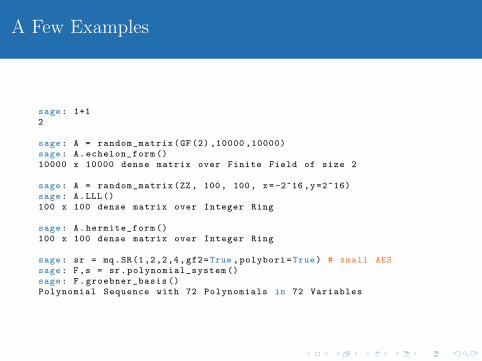
A Few Examples

sage: 1+12

sage: A = random_matrix(GF (2) ,10000 ,10000)sage: A.echelon_form ()10000 x 10000 dense matrix over Finite Field of size 2

sage: A = random_matrix(ZZ , 100, 100, x=-2^16,y=2^16)sage: A.LLL()100 x 100 dense matrix over Integer Ring

sage: A.hermite_form ()100 x 100 dense matrix over Integer Ring

sage: sr = mq.SR(1,2,2,4,gf2=True ,polybori=True) # small AESsage: F,s = sr.polynomial_system ()sage: F.groebner_basis ()Polynomial Sequence with 72 Polynomials in 72 Variables

Blurb

Sage open-source mathematical software system

“Creating a viable free open source alternative toMagma, Maple, Mathematica and Matlab.”

Sage is a free open-source mathematics software system licensedunder the GPL. It combines the power of many existing open-sourcepackages into a common Python-based interface.

First release 2005 Latest version 5.0 released 2012-05-14> 300 Releases Shell, webbrowser (GUI), library> 180 Developers ∼ 100 Components> 100 papers cite Sage > 2100 subscribers [sage-support]> 100,000 web visitors/month > 6, 500 downloads/month

How to use it

Sage can be used via the command line, as a webapp hosted on yourlocal computer and via the Internet, or embedded on any website.

“How do I do . . . in Sage?”. . . It’s easy: implement it and send us a patch.

Sage is a largely volunteer-driven effort, this means that

developers work on whatever suits their needs best;

the quality of code in Sage varies:

is a generic or a specialised, optimised implementation used,how much attention is paid to details,is your application an untested “corner case”,how extensive are the tests, the documentation, oris the version of a particular package up to date.

you cannot expect people to fix your favourite bug quickly(although we do try!),

you can get involved and make Sage better for your needs!

Get involved

I will highlight relevant issues to encourage you to get involved.

Outline

1 Introduction


3 Mathematics

4 Cryptography



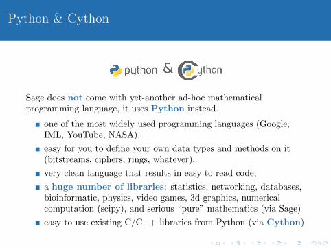
Python & Cython

Sage does not come with yet-another ad-hoc mathematicalprogramming language, it uses Python instead.

one of the most widely used programming languages (Google,IML, YouTube, NASA),

easy for you to define your own data types and methods on it(bitstreams, ciphers, rings, whatever),

very clean language that results in easy to read code,

a huge number of libraries: statistics, networking, databases,bioinformatic, physics, video games, 3d graphics, numericalcomputation (scipy), and serious “pure” mathematics (via Sage)

easy to use existing C/C++ libraries from Python (via Cython)

Python Example: Databases

sage: import sqlalchemy as Ssage: db = S.create_engine(’sqlite :/// tutorial.db’)sage: users = S.Table(’users’, S.MetaData(db),

S.Column(’user_id ’, S.Integer , primary_key=True),S.Column(’name’, S.String (40r)),S.Column(’modulus ’, S.String )). create ()

sage: i = users.insert ()sage: M = random_prime (2^512)* random_prime (2^512)sage: i.execute(name=’Mary’,modulus=str(M))

sage: s = users.select(whereclause="name=’Mary’")sage: row = s.execute (). fetchone ()sage: ZZ(row[users.c.modulus ])56974631402866323...250077669

Python Example: Networking

Scapy is a powerful interactive packet manipulation program written in

Python. It is able to forge or decode packets of a wide number of protocols,

send them on the wire, capture them, match requests and replies, and much

more. It can easily handle most classical tasks like scanning, tracerouting,

probing, unit tests, attacks or network discovery.

from scapy.all import *

class Test(Packet ):name = "Test packet"fields_desc = [ ShortField("test1", 1),

ShortField("test2", 2) ]

print Ether ()/IP()/ Test(test1=x,test2=y)

p=sr1(IP(dst="127.0.0.1")/ICMP ())if p:

p.show()

Cython: Your Own Code

sage: cython("""def foo(unsigned long a, unsigned long b):

cdef int ifor i in range (64):

a ^= a*(b<<i)return a

""")sage: foo(a,b)

This generates C code like this:

for (__pyx_t_1 = 0; __pyx_t_1 < 64; __pyx_t_1 +=1) {__pyx_v_i = __pyx_t_1;__pyx_v_a = (__pyx_v_a ^ _pyx_v_a * (__pyx_v_b << __pyx_v_i ));

}

Cython: External Code I

#cargs -std=c99 -ggdbcdef extern from "katan.c":

ctypedef unsigned long uint64_tvoid katan32_encrypt(uint64_t *p, uint64_t *c, uint64_t *k, int nr)void katan32_keyschedule(uint64_t *k, uint64_t *key , int br)uint64_t ONES

def k32_encrypt(plain , key):cdef int icdef uint64_t _plain [32], _cipher [32], kk[2*254] , _key [80]

for i in range (80):_key[i] = ONES if key[i] else 0

for i in range (32):_plain[i] = ONES if plain[i] else 0

katan32_keyschedule(kk, _key , 254)katan32_encrypt(_plain , _cipher , _key , 254)

return [int(_cipher[i]%2) for i in range (32)]

sage: attach "sage -katan.spyx"sage: k32_encrypt(random_vector(GF(2),32), random_vector(GF(2) ,80))[1, 0, 0, 1, 0, 1, 0, 0, 0, 1, ... 0, 1, 0, 0]

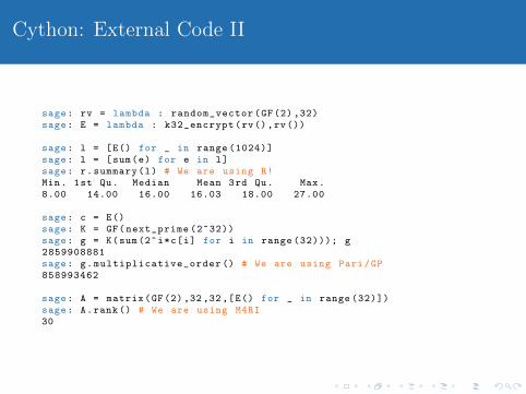
Cython: External Code II

sage: rv = lambda : random_vector(GF(2) ,32)sage: E = lambda : k32_encrypt(rv(),rv())

sage: l = [E() for _ in range (1024)]sage: l = [sum(e) for e in l]sage: r.summary(l) # We are using R!Min. 1st Qu. Median Mean 3rd Qu. Max.8.00 14.00 16.00 16.03 18.00 27.00

sage: c = E()sage: K = GF(next_prime (2^32))sage: g = K(sum(2^i*c[i] for i in range (32))); g2859908881sage: g.multiplicative_order () # We are using Pari/GP858993462

sage: A = matrix(GF(2),32,32,[E() for _ in range (32)])sage: A.rank() # We are using M4RI30

Symmetric Multiprocessing

Embarrassingly proudly parallel computations on multicore machinesare easy in Sage:

sage: @parallel (2)....: def f(n):....: return factor(n)....:

sage: %time _ = [f(2^217 -1) , f(2^217 -1)]CPU times: user 1.07 s, sys: 0.02 s, total: 1.09 sWall time: 1.10 s

sage: %time _ = list( f([2^217 -1 , 2^217 -1]) )CPU times: user 0.00 s, sys: 0.02 s, total: 0.02 sWall time: 0.62 s

sage: 1.08/0.621.74193548387097

Outline

1 Introduction


3 Mathematics

4 Cryptography



Dense Linear Algebra I

Base Ring Implementation CommentsF2e 1 ≤ e ≤ 10 M4RI, M4RIE Very goodFp, p = 3, 5, 7, . . . LinBox DecentFp, p < 222 prime LinBox Very goodFpk Generic Very poor

Q,Z LinBox, Pari, IML, NTL, custom Decent, fastest HNFR,C 53-bit NumPy + ATLAS Very goodQ(ζn) Custom Very goodK[x] Generic Very poorK[x0, . . . , xn−1] Singular, generic Mixed

Dense Linear Algebra II

sage: for p in (2,3,4,5,7,8,9,11):....: K = GF(p,’a’)....: A = random_matrix(K ,2000 ,2000)....: B = random_matrix(K ,2000 ,2000)....: t = cputime ()....: C = A*B....: print "%32s %7.3f"%(K,cputime(t))....:Finite Field of size 2 0.008 # M4RIFinite Field of size 3 0.972 # LinBoxFinite Field in a of size 2^2 0.048 # M4RIEFinite Field of size 5 0.996 # LinBoxFinite Field of size 7 0.968 # LinBoxFinite Field in a of size 2^3 0.072 # M4RIEFinite Field in a of size 3^2 695.863 # genericFinite Field of size 11 1.020 # LinBox

Get Involved!

We are currently working on improving Fpk . FLINT 2.3 improves Fp

for p < 264.

Sparse Linear Algebra

Sage allows to construct and to compute with sparse matrices usingthe sparse=True keyword.

sage: A = random_matrix(GF(32003) ,2000 ,2000 , density =~200 , sparse=True)sage: %time copy(A).rank() # LinBoxCPU times: user 3.26 s, sys: 0.05 s, total: 3.31 sWall time: 3.33 s2000sage: %time copy(A). echelonize () # custom codeCPU times: user 9.51 s, sys: 0.02 s, total: 9.52 sWall time: 9.56 ssage: v = random_vector(GF (32003) ,2000)sage: %time _ = copy(A). solve_right(v) # LinBox + custom codeCPU times: user 3.74 s, sys: 0.00 s, total: 3.74 sWall time: 3.76 s

Get Involved!

LinBox’s claim to fame is good support for black box algorithms forsparse and structured matrices. Help us to expose more of thisfunctionality.

Lattices I

Sage includes both NTL and fpLLL:

sage: from sage.libs.fplll.fplll import gen_intrel # Knapsack -stylesage: A = gen_intrel (50 ,50); A50 x 51 dense matrix over Integer Ring ...sage: min(v.norm ().n() for v in A.rows ())2.17859318110950 e13

sage: L = A.LLL() # using fpLLL , NTL optionalsage: L[0]. norm ().n()5.47722557505166

sage: L = A.BKZ() # using NTLsage: L[0]. norm ().n()3.60555127546399

Lattices II

Coppersmith’s method for finding small roots is available:

sage: N = 10001sage: K = Zmod (10001)sage: P.<x> = PolynomialRing(K)sage: f = x^3 + 10*x^2 + 5000*x - 222sage: f.small_roots ()[4]

Get Involved!

our version of fpLLL is very old,

fpLLL 4.0 has an implementation of BKZ, and

there is no Lattice class for e.g. L.shortest vector(gap=x),

but improving this is a Google Summer of Code 2012 project.

Combinatorics

sage: IV3 = IntegerVectors (3,10)sage: IV3.random_element ()[0, 0, 1, 0, 0, 2, 0, 0, 0, 0]

sage: C = Combinations(range (100) ,10); CCombinations of [0, 1, 2, 3, 4, ..., 98, 99] of length 10sage: C.cardinality ()17310309456440

Sage also has a very active (algebraic) combinatorics group.

You can tell by the lack of examples how badly I suck atcombinatorics . . . there’s lots and lots in Sage.

Symbolics

Sage uses Pynac (GiNaC fork) and Maxima for most of its symbolicmanipulation. SymPy is included in Sage as well.

sage: q = var(’q’)sage: expr = (1-1/q)/(q-1)sage: f = expr.function(q); fq |--> -(1/q - 1)/(q - 1)sage: f(10)1/10sage: f(q^2)-(1/q^2 - 1)/(q^2 - 1)sage: f(0.1)10.0000000000000sage: g = P.random_element (); g4*x^2 + 3/4*xsage: f(g)-4*(4/((16*x + 3)*x) - 1)/((16*x + 3)*x - 4)

sage: expr.simplify_full ()1/qsage: expr.integrate(q)log(q)

Numerical Root Finding and Approximation I

Assume, we want have two counters: one for a correct key guess andone for an incorrect guess. Assume further that these counters aredistributed according N (Ec,Varc) and N (Ew,Varw). We want toknow how many samples we need to distinguish these twodistributions for 50% of the keys. That is, we want to solve

1− en <1

2

(1 + erf

(Ec(n)− Ew(n)√

2Varw(n)/m

))for m.

Numerical Root Finding and Approximation II

First, we compute some data by numerically solving for m:

sage: n,m = var(’n,m’)...sage: f = 1/2 * (1 + erf( (E_c(n,m) - E_w(n,m))/

(sqrt (2* Var_w(n,m))) ) - (1 - e^n)sage: l = []sage: for n in range (64 ,256+1 ,8):... f_n = f.subs(n=n). function(m)... m = ceil(f_n.find_root (32 ,2**40)... l.append( (n,m) )

Numerical Root Finding and Approximation III

Now, we approximate this data numerically under the assumptionthat m = poly(n)

sage: n,c,a,b = var(’n,c,a,b’)sage: model = (a*n**c + b). function(n)sage: s = find_fit(l, model , solution_dict=True)sage: m = model.subs(s); mn |--> 0.021639206984895312*n^1.5496891146692116 + 89.975123416726277

Hence, we have m ≈ 0.022 · n1.55 + 90.

Statistics I

Sage ships R which is a very powerful package for doing statistics,Sage also uses SciPy for stats related tasks.

sage: O() # some oraclesage: l = [O() for _ in range (10000)] # we sample itsage: r.summary(l) # and ask R about it

Min. 1st Qu. Median Mean 3rd Qu. Max.-154.000 -31.000 2.000 0.298 33.000 140.000sage: import pylab # use pylab to compute a histogramsage: a,b,_ = pylab.hist(l,100)sage: line(zip(b,a)) # and Sage’s code to plot it

Get Involved!

Our interface to R could be greatlyimproved

Statistics II

Looks kinda Gaussian, doesn’t it.

sage: T = RealDistribution(’gaussian ’,variance(l).sqrt ())sage: T.cum_distribution_function (5)0.542044391014

sage: mu = mean(l)sage: len([e for e in l if e<5+mu])/ float(len(l))0.53839999999999999

Group Theory I

Sage supports operations such as discrete logarithms on genericgroups.

sage: A = matrix(GF (50021) ,[[10577 ,23999 ,28893] ,[14601 ,41019 ,30188] ,[3081, 736 ,27092]])

sage: discrete_log_rho(A^1324234 ,A)1324234

Sage also includes GAP which provides high-quality group theory.

sage: G = PermutationGroup ([(1,2,3), (2 ,3)])sage: N = PermutationGroup ([(1 ,2 ,3)])sage: G.quotient(N)Permutation Group with generators [(1 ,2)]

Factoring

factor uses Pari

sage: %time factor(next_prime (2^40) * next_prime (2^300))CPU times: user 2.39 s, sys: 0.00 s, total: 2.39 sWall time: 2.41 s1099511627791 * 203703597633448608626...

ecm uses GMP-ECM

sage: %time ecm.factor(next_prime (2^40) * next_prime (2^300))CPU times: user 0.11 s, sys: 0.01 s, total: 0.12 sWall time: 0.82 s[1099511627791 , 203703597633448608626...

qsieve uses Bill Hart’s qsieve implementation

sage: p, q = next_prime (2^90) , next_prime (2^91)sage: v,t = qsieve(p*q,time=True); t[:4]2.26

Get Involved!

These should be unified to one command.

Elliptic Curves I

Sage is pretty good over Qsage: E = EllipticCurve("37a")sage: show(E.plot ())

. . . and okay over Fp

sage: E = E.change_ring(GF (997))sage: show(E.plot ())

Elliptic Curves II

Basic operations over Fp are available

sage: k = GF(next_prime (10^7))sage: E = EllipticCurve(k, (k.random_element (),k.random_element ()))sage: EElliptic Curve defined by y^2 = x^3 + 7736620*x + 5470618over Finite Field of size 10000019sage: P = E.random_element ()sage: P.order()499712sage: 2*P + 1(1070248 : 6510834 : 1)

Elliptic Curves III

Sage includes a fast implementation of the SEA (Schoff-Elkies-Atkin)algorithm for counting the number of points on an elliptic curve overFp.

sage: K = GF(next_prime (10^20))sage: E = EllipticCurve_from_j(k.random_element ())sage: E.cardinality ()99999999999371984255

Sage has the world’s best code for computing p-adic regulators ofelliptic curves. The p-adic regulator of an elliptic curve E at a goodordinary prime p is the determinant of the global p-adic height pairingmatrix on the Mordell-Weil group E(Q).

sage: E = EllipticCurve(’389a’)sage: E.padic_regulator (5, 10)5^2 + 2*5^3 + 2*5^4 + 4*5^5 + 3*5^6 + 4*5^7 + 3*5^8 + 5^9 + O(5^11)sage: E.padic_regulator (997, 10)740*997^2 + 916*997^3 + 472*997^4 + 325*997^5 + 697*997^6

+ 642*997^7 + 68*997^8 + 860*997^9 + 884*997^10 + O(997^11)

Elliptic Curves IV

Sage has the world’s fastest implementation of computation of allintegral points on an elliptic curve over Q. This is also the only freeopen-source implementation available.

(Apparently,) a very impressive example is the lowest conductorelliptic curve of rank 3, which has 36 integral points.

sage: E = elliptic_curves.rank (3)[0]sage: E.integral_points(both_signs=True) # less than 3 seconds[(-3 : -1 : 1), (-3 : 0 : 1), ...(816 : -23310 : 1), (816 : 23309 : 1)]

Grobner Bases I

sage: K = GF (32003)sage: T = TermOrder("deglex" ,2) + TermOrder("deglex" ,2)sage: P.<w,x,y,z> = PolynomialRing(K,order=T)sage: I = sage.rings.ideal.Katsura(P)sage: [g.lm() for g in I.groebner_basis ()] # Singular[w, x, y*z^3, z^4, y^3, y^2*z]sage: I.dimension ()0sage: V = I.variety (); V[{y: 0, z: 0, w: 1, x: 0}, {y: 0, z: 10668, w: 10668, x: 0}]sage: J = I.change_ring(P.change_ring(QQ))sage: J.variety ()[{y: 0, z: -32002/3, w: -32002/3, x: 0}, {y: 0, z: 0, w: -32002, x: 0}]sage: len(J.variety(CC))8

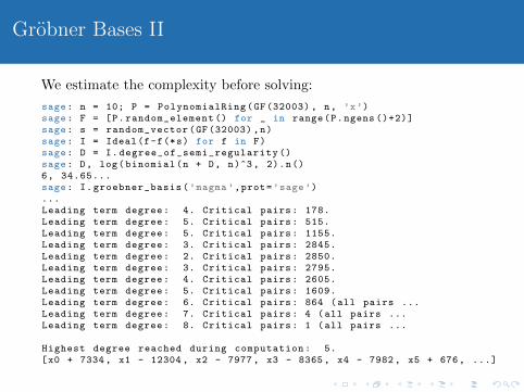
Grobner Bases II

We estimate the complexity before solving:

sage: n = 10; P = PolynomialRing(GF(32003) , n, ’x’)sage: F = [P.random_element () for _ in range(P.ngens ()+2)]sage: s = random_vector(GF(32003) ,n)sage: I = Ideal(f-f(*s) for f in F)sage: D = I.degree_of_semi_regularity ()sage: D, log(binomial(n + D, n)^3, 2).n()6, 34.65...sage: I.groebner_basis(’magma ’,prot=’sage’)...Leading term degree: 4. Critical pairs: 178.Leading term degree: 5. Critical pairs: 515.Leading term degree: 5. Critical pairs: 1155.Leading term degree: 3. Critical pairs: 2845.Leading term degree: 2. Critical pairs: 2850.Leading term degree: 3. Critical pairs: 2795.Leading term degree: 4. Critical pairs: 2605.Leading term degree: 5. Critical pairs: 1609.Leading term degree: 6. Critical pairs: 864 (all pairs ...Leading term degree: 7. Critical pairs: 4 (all pairs ...Leading term degree: 8. Critical pairs: 1 (all pairs ...

Highest degree reached during computation: 5.[x0 + 7334, x1 - 12304 , x2 - 7977, x3 - 8365, x4 - 7982, x5 + 676, ...]

Grobner Bases III

Sage has a very good implementation of Grobner basis computationsover F2[x0, . . . , xn−1]/〈x2

0 + x0, . . . , x2n−1 + xn−1〉 thanks to PolyBoRi.

sage: B = BooleanPolynomialRing (50,’x’,order=’deglex ’)sage: s = random_vector(GF(2) ,50)sage: F = [B.random_element () for _ in range (500)]sage: I = Ideal(f-f(*s) for f in F)sage: G = I.groebner_basis (); G # PolyBoRiPolynomial Sequence with 50 Polynomials in 50 Variablessage: sorted(G)[0], s[0](x0 + 1, 1)sage: I.variety ()[{x40: 0, x42: 1, x44: 0, ..., x23: 0, x25: 1}]

Mixed/Constraint Integer Programming I

Sage has a highlevel interface to Mixed Integer Linear solving

sage: g = graphs.PetersenGraph ()sage: p = MixedIntegerLinearProgram(maximization=True)sage: b = p.new_variable ()sage: p.set_objective(sum([b[v] for v in g]))sage: for (u,v) in g.edges(labels=None):... p.add_constraint(b[u] + b[v], max=1)sage: p.set_binary(b)sage: p.solve(objective_only=True)4.0

which supports many backends: GLPK, Coin, Gurobi, CPLEX.

Get Involved!

There is a patch bitrotting which adds a SCIP interface to Sage.There’s also some code which converts polynomial systems (withnoise) to MIP/CIP awaiting integration into Sage.

Graph Theory

builds on NetworkX (Los Alamos’s Python graph library)

graph isomorphism testing – Robert Miller’s new implementation

graph databases

2d and 3d visualization

sage: D = graphs.DodecahedralGraph ()sage: D.show3d ()

sage: E = D.copy()sage: gamma = SymmetricGroup (20). random_element ()sage: E.relabel(gamma)sage: D.is_isomorphic(E)Truesage: D.radius ()5

Outline

1 Introduction


3 Mathematics

4 Cryptography



AES & Equation Systems I

We construct small scale AES – SR(1,1,1,4) – over F24

sage: sr = mq.SR(1,1,1,4); srSR(1,1,1,4)sage: F,s = sr.polynomial_system () #zero inversions...<type ’exceptions.ZeroDivisionError ’>: A zero inversion occurred ...

sage: F,s = sr.polynomial_system (); F # So we try again.Polynomial System with 40 Polynomials in 20 Variables

AES & Equation Systems II

We can export F to Magma:

sage: magma(F)Ideal of Polynomial ring of rank 20 over GF (2^4)Graded Reverse Lexicographical OrderVariables: k100 , k101 , k102 , k103 , x100 , x101 , x102 , x103 , ...Basis:[w100 + k000 + $.1^4,w101 + k001 + $.1^8,...k000^2 + k001 ,....

or to Singular:

sage: singular(F)w100+k000+(a+1),w101+k001+(a^2+1),...k002 ^2+k003 ,...

AES & Equation Systems III

Or we can use those systems transparently in the background:

sage: F.groebner_basis () # Singular in the background[k002 + (a^3 + 1)* k003 + (a^2),k001 + (a^3 + a^2)* k003 + (a^3),k000 + (a^2)* k003 + (a^3 + a^2),...

sage: F.groebner_basis(algorithm=’magma ’) # Magma in the background[k002 + (a^3 + 1)* k003 + (a^2),k001 + (a^3 + a^2)* k003 + (a^3),k000 + (a^2)* k003 + (a^3 + a^2),...

AES & Equation Systems IV

Building blocks are also available individually:

sage: sr.Lin[ a^2 + 1 1 a^3 + a^2 a^2 + 1][ a a 1 a^3 + a^2 + a + 1][ a^3 + a a^2 a^2 1][ 1 a^3 a + 1 a + 1]

sage: sr = mq.SR(1, 1, 1, 8)sage: R = sr.ring()sage: xi = Matrix(R, 8, 1, sr.vars(’x’, 1))sage: wi = Matrix(R, 8, 1, sr.vars(’w’, 1))sage: sr.inversion_polynomials(xi , wi, 8)[x100*w100 + 1, x101*w101 + 1, x102*w102 + 1, x103*w103 + 1,x104*w104 + 1, x105*w105 + 1, x106*w106 + 1, x107*w107 + 1]

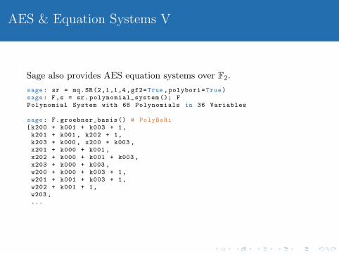
AES & Equation Systems V

Sage also provides AES equation systems over F2.

sage: sr = mq.SR(2,1,1,4,gf2=True ,polybori=True)sage: F,s = sr.polynomial_system (); FPolynomial System with 68 Polynomials in 36 Variables

sage: F.groebner_basis () # PolyBoRi[k200 + k001 + k003 + 1,k201 + k001 , k202 + 1,k203 + k000 , x200 + k003 ,x201 + k000 + k001 ,x202 + k000 + k001 + k003 ,x203 + k000 + k003 ,w200 + k000 + k003 + 1,w201 + k001 + k003 + 1,w202 + k001 + 1,w203 ,...

AES & Equation Systems VI

Interdependencies between polynomials:

sage: sr = mq.SR(1,4,4,4,gf2=True ,polybori=True , \allow_zero_inversions=True)

sage: F,s = sr.polynomial_system ()sage: F_short = mq.MPolynomialSystem(F.ring(), F.rounds ()[: -1])sage: F_short.connected_components ()[Polynomial System with 80 Polynomials in 64 Variables ,Polynomial System with 80 Polynomials in 64 Variables ,Polynomial System with 80 Polynomials in 64 Variables ,Polynomial System with 80 Polynomials in 64 Variables]

sage: S = mq.SBox (12,5,6,11,9,0,10,13,3,14,15,8,4,7,1,2)sage: F_S = mq.MPolynomialSystem(S.polynomials(degree=3,groebner=True))sage: F_S.connection_graph ()Graph on 8 vertices

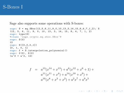
S-Boxes I

Sage also supports some operations with S-boxes:

sage: S = mq.SBox (12,5,6,11,9,0,10,13,3,14,15,8,4,7,1,2); S(12, 5, 6, 11, 9, 0, 10, 13, 3, 14, 15, 8, 4, 7, 1, 2)sage: type(S)<class ’sage.crypto.mq.sbox.SBox’>sage: S(0)12sage: S([0,0,0,1])[0, 1, 0, 1]sage: f = S.interpolation_polynomial ()sage: f(0), S(0)(a^3 + a^2, 12)

f = a13(x14 + x13) + a6(x12 + x6 + 1) +

a11(x11 + x4) + a14(x10 + x9) +

a10(x8 + x3 + x2) + a2x7 + a9x5

S-Boxes II

sage: S = mq.SBox (12,5,6,11,9,0,10,13,3,14,15,8,4,7,1,2)sage: S.linear_approximation_matrix ()[ 8 0 0 0 0 0 0 0 0 0 0 0 0 0 0 0][ 0 0 0 0 0 -4 0 -4 0 0 0 0 0 -4 0 4][ 0 0 2 2 -2 -2 0 0 2 -2 0 4 0 4 -2 2][ 0 0 2 2 2 -2 -4 0 -2 2 -4 0 0 0 -2 -2][ 0 0 -2 2 -2 -2 0 4 -2 -2 0 -4 0 0 -2 2][ 0 0 -2 2 -2 2 0 0 2 2 -4 0 4 0 2 2][ 0 0 0 -4 0 0 -4 0 0 -4 0 0 4 0 0 0][ 0 0 0 4 4 0 0 0 0 -4 0 0 0 0 4 0][ 0 0 2 -2 0 0 -2 2 -2 2 0 0 -2 2 4 4][ 0 4 -2 -2 0 0 2 -2 -2 -2 -4 0 -2 2 0 0][ 0 0 4 0 2 2 2 -2 0 0 0 -4 2 2 -2 2][ 0 -4 0 0 -2 -2 2 -2 -4 0 0 0 2 2 2 -2][ 0 0 0 0 -2 -2 -2 -2 4 0 0 -4 -2 2 2 -2][ 0 4 4 0 -2 -2 2 2 0 0 0 0 2 -2 2 -2][ 0 0 2 2 -4 4 -2 -2 -2 -2 0 0 -2 -2 0 0][ 0 4 -2 2 0 0 -2 -2 -2 2 4 0 2 2 0 0]

S-Boxes III

sage: S = mq.SBox (12,5,6,11,9,0,10,13,3,14,15,8,4,7,1,2)sage: S.difference_distribution_matrix ()[16 0 0 0 0 0 0 0 0 0 0 0 0 0 0 0][ 0 0 0 4 0 0 0 4 0 4 0 0 0 4 0 0][ 0 0 0 2 0 4 2 0 0 0 2 0 2 2 2 0][ 0 2 0 2 2 0 4 2 0 0 2 2 0 0 0 0][ 0 0 0 0 0 4 2 2 0 2 2 0 2 0 2 0][ 0 2 0 0 2 0 0 0 0 2 2 2 4 2 0 0][ 0 0 2 0 0 0 2 0 2 0 0 4 2 0 0 4][ 0 4 2 0 0 0 2 0 2 0 0 0 2 0 0 4][ 0 0 0 2 0 0 0 2 0 2 0 4 0 2 0 4][ 0 0 2 0 4 0 2 0 2 0 0 0 2 0 4 0][ 0 0 2 2 0 4 0 0 2 0 2 0 0 2 2 0][ 0 2 0 0 2 0 0 0 4 2 2 2 0 2 0 0][ 0 0 2 0 0 4 0 2 2 2 2 0 0 0 2 0][ 0 2 4 2 2 0 0 2 0 0 2 2 0 0 0 0][ 0 0 2 2 0 0 2 2 2 2 0 0 2 2 0 0][ 0 4 0 0 4 0 0 0 0 0 0 0 0 0 4 4]

S-Boxes IV

sage: S = mq.SBox (12,5,6,11,9,0,10,13,3,14,15,8,4,7,1,2)sage: S.polynomials () #default: degree =2[x1*x2 + x0 + x1 + x3 + y3,x0*x1 + x0*x2 + x0 + x1 + y0 + y2 + y3 + 1,x0*x3 + x1*x3 + x1*y0 + x0*y1 + x0*y2 + x1 + x2 + y2,x0*x3 + x0*y0 + x1*y1 + x0 + x2 + y2,x0*x2 + x0*y0 + x0*y1 + x1*y2 + x1 + x2 + x3 + y2 + y3, ...]

sage: S = mq.SBox (12,5,6,11,9,0,10,13,3,14,15,8,4,7,1,2)sage: P.<y0,y1 ,y2,y3 ,x0,x1,x2 ,x3> = PolynomialRing(GF(2),order=’lex’)sage: X = [x0,x1 ,x2,x3]sage: Y = [y0,y1 ,y2,y3]sage: S.polynomials(X=X,Y=Y,degree=3,groebner=True)[y0 + x0*x1*x3 + x0*x2*x3 + x0 + x1*x2*x3 + x1*x2 + x2 + x3 + 1,y1 + x0*x1*x3 + x0*x2*x3 + x0*x2 + x0*x3 + x0 + x1 + x2*x3 + 1,y2 + x0*x1*x3 + x0*x1 + x0*x2*x3 + x0*x2 + x0 + x1*x2*x3 + x2,y3 + x0 + x1*x2 + x1 + x3]

Boolean Functions I

sage: from sage.crypto.boolean_function import *sage: P.<x0,x1 ,x2,x3 > = BooleanPolynomialRing ()sage: b = x0*x1 + x2*x3sage: f = BooleanFunction(b)sage: [b(x[0],x[1],x[2],x[3]) for x in GF (2)^4][0, 0, 0, 1, 0, 0, 0, 1, 0, 0, 0, 1, 1, 1, 1, 0]sage: f.truth_table ()(False , False , False , True , False , False , False , True , False , False ,False , True , True , True , True , False)

Boolean Functions II

sage: WT = f.walsh_hadamard_transform (); WT(-4, -4, -4, 4, -4, -4, -4, 4, -4, -4, -4, 4, 4, 4, 4, -4)sage: f.absolute_walsh_spectrum (){4: 16}sage: f.nonlinearity ()6sage: 2^(4 -1) - (1/2)* max([abs(x) for x in WT])6

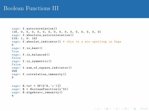
Boolean Functions III

sage: f.autocorrelation ()(16, 0, 0, 0, 0, 0, 0, 0, 0, 0, 0, 0, 0, 0, 0, 0)sage: f.absolute_autocorrelation (){16: 1, 0: 15}sage: f.absolut_indicator () # this is a mis -spelling in Sage0sage: f.is_bent ()Truesage: f.is_balanced ()Falsesage: f.is_symmetric ()Falsesage: f.sum_of_square_indicator ()256sage: f.correlation_immunity ()0

sage: R.<x> = GF(2^8,’a’)[]sage: B = BooleanFunction(x^31)sage: B.algebraic_immunity ()4

Lattice Generators I

Sage can generate many crypto-style lattices thanks to RichardLindner and Michael Schneider.

Modular basis

sage: sage.crypto.gen_lattice(m=10, seed =42)[11 0 0 0 0 0 0 0 0 0][ 0 11 0 0 0 0 0 0 0 0][ 0 0 11 0 0 0 0 0 0 0][ 0 0 0 11 0 0 0 0 0 0][ 2 4 3 5 1 0 0 0 0 0][ 1 -5 -4 2 0 1 0 0 0 0][-4 3 -1 1 0 0 1 0 0 0][-2 -3 -4 -1 0 0 0 1 0 0][-5 -5 3 3 0 0 0 0 1 0][-4 -3 2 -5 0 0 0 0 0 1]

Lattice Generators II

Random basis

sage: sage.crypto.gen_lattice(type=’random ’,n=1,m=10,q=11^4 , seed =42)[14641 0 0 0 0 0 0 0 0 0][ 431 1 0 0 0 0 0 0 0 0][-4792 0 1 0 0 0 0 0 0 0][ 1015 0 0 1 0 0 0 0 0 0][-3086 0 0 0 1 0 0 0 0 0][-5378 0 0 0 0 1 0 0 0 0][ 4769 0 0 0 0 0 1 0 0 0][-1159 0 0 0 0 0 0 1 0 0][ 3082 0 0 0 0 0 0 0 1 0][-4580 0 0 0 0 0 0 0 0 1]

Lattice Generators III

Ideal bases with quotient xn − 1, m = 2n are NTRU bases

sage: sage.crypto.gen_lattice(type=’ideal’, seed=42, quotient=x^4-1)[11 0 0 0 0 0 0 0][ 0 11 0 0 0 0 0 0][ 0 0 11 0 0 0 0 0][ 0 0 0 11 0 0 0 0][ 4 -2 -3 -3 1 0 0 0][-3 4 -2 -3 0 1 0 0][-3 -3 4 -2 0 0 1 0]

Lattice Generators IV

Cyclotomic bases with n = 2k are SWIFFT bases

sage: sage.crypto.gen_lattice(type=’cyclotomic ’, seed =42)[11 0 0 0 0 0 0 0][ 0 11 0 0 0 0 0 0][ 0 0 11 0 0 0 0 0][ 0 0 0 11 0 0 0 0][ 4 -2 -3 -3 1 0 0 0][ 3 4 -2 -3 0 1 0 0][ 3 3 4 -2 0 0 1 0][ 2 3 3 4 0 0 0 1]

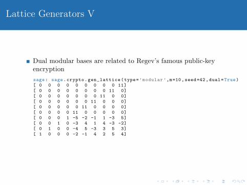
Lattice Generators V

Dual modular bases are related to Regev’s famous public-keyencryption

sage: sage.crypto.gen_lattice(type=’modular ’,m=10,seed=42,dual=True)[ 0 0 0 0 0 0 0 0 0 11][ 0 0 0 0 0 0 0 0 11 0][ 0 0 0 0 0 0 0 11 0 0][ 0 0 0 0 0 0 11 0 0 0][ 0 0 0 0 0 11 0 0 0 0][ 0 0 0 0 11 0 0 0 0 0][ 0 0 0 1 -5 -2 -1 1 -3 5][ 0 0 1 0 -3 4 1 4 -3 -2][ 0 1 0 0 -4 5 -3 3 5 3][ 1 0 0 0 -2 -1 4 2 5 4]

Outline

1 Introduction


3 Mathematics

4 Cryptography



DES I

An equation system generator for DES is available athttp://bitbucket.org/malb/algebraic_attacks.

sage: attach des.pysage: des = DES(Nr=2,sbox_eq=’cubic’) #sopns , sopns_gbsage: F,s = des.polynomial_system ()Pre -computing fully cubic S-Box equations.sage: FPolynomial System with 1856 Polynomials in 120 Variablessage: F_easy = F.subs(s); F_easyPolynomial System with 1856 Polynomials in 64 Variablessage: %time gb = F_easy.groebner_basis ()CPU times: user 0.20 s, sys: 0.01 s, total: 0.22 sWall time: 0.32 ssage: gb[:5][y0100 , y0101 , y0102 , y0103 + 1, y0104]

sage: %time gb = F.groebner_basis ()CPU times: user 0.42 s, sys: 0.00 s, total: 0.42 sWall time: 0.47 ssage: gb[:5][k00 + 1, k01 , k02 , k03 + 1, k04 + 1]

http://bitbucket.org/malb/algebraic_attacks

DES II

S-boxes are available independently:

sage: S1 = DESSBox (1)sage: S1.polynomials(degree =3)... # a long long listsage: print S1.difference_distribution_matrix (). str()[64 0 0 0 0 0 0 0 0 0 0 0 0 0 0 0][ 0 0 0 6 0 2 4 4 0 10 12 4 10 6 2 4][ 0 0 0 8 0 4 4 4 0 6 8 6 12 6 4 2][14 4 2 2 10 6 4 2 6 4 4 0 2 2 2 0][ 0 0 0 6 0 10 10 6 0 4 6 4 2 8 6 2][ 4 8 6 2 2 4 4 2 0 4 4 0 12 2 4 6][ 0 4 2 4 8 2 6 2 8 4 4 2 4 2 0 12][ 2 4 10 4 0 4 8 4 2 4 8 2 2 2 4 4][ 0 0 0 12 0 8 8 4 0 6 2 8 8 2 2 4][10 2 4 0 2 4 6 0 2 2 8 0 10 0 2 12][ 0 8 6 2 2 8 6 0 6 4 6 0 4 0 2 10][ 2 4 0 10 2 2 4 0 2 6 2 6 6 4 2 12][ 0 0 0 8 0 6 6 0 0 6 6 4 6 6 14 2]...

PRESENT

An equation system generator for PRESENT is also available.

sage: attach present.pysage: p = PRESENT(Nr=1)sage: F,s = p.polynomial_system (); FPolynomial System with 502 Polynomials in 212 Variablessage: R = F.ring()sage: R.gens ()[:16](K0000 , K0001 , K0002 , K0003 , K0004 , K0005 , K0006 , ...)sage: K_guess = R.gens ()[:16] # 80 - 64 = 16sage: guess = dict ([(k,GF(2). random_element ()) for k in K_guess ])sage: F_guessed = F.subs(guess); F_guessedPolynomial System with 502 Polynomials in 196 Variablessage: F_target = F_guessed.eliminate_linear_variables ()sage: F_targetPolynomial System with 260 Polynomials in 42 Variablessage: F_target.groebner_basis ()[1]

sage: guess = dict ([(k,s[k]) for k in K_guess ])sage: F_guessed = F.subs(guess)sage: F_target = F_guessed.eliminate_linear_variables ();sage: gb = F_target.groebner_basis ()sage: gb[-1]K0070

Outline

1 Introduction


3 Mathematics

4 Cryptography



LWE in 10 lines

sage: n = 10sage: q = random_prime(n^2,2*n^2); K = GF(q)sage: VS = VectorSpace(K,n)sage: s = VS.random_element ()sage: chi = lambda: K(round(gauss(0,sqrt(n))))sage: def sample ():....: a = VS.random_element ()....: return a, a.dot_product(s)+chi()....:sage: sample ()((3, 7, 7, 0, 12, 6, 13, 15, 15, 10), 5)

O. Regev.The learning with errors problem.In IEEE Conf. on Comp. Complexity 2010, pages 191–204, 2010.

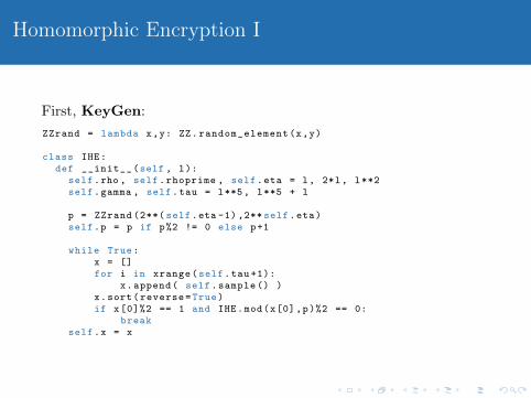
Homomorphic Encryption I

First, KeyGen:

ZZrand = lambda x,y: ZZ.random_element(x,y)

class IHE:def __init__(self , l):

self.rho , self.rhoprime , self.eta = l, 2*l, l**2self.gamma , self.tau = l**5, l**5 + l

p = ZZrand (2**( self.eta -1) ,2** self.eta)self.p = p if p%2 != 0 else p+1

while True:x = []for i in xrange(self.tau +1):

x.append( self.sample () )x.sort(reverse=True)if x[0]%2 == 1 and IHE.mod(x[0],p)%2 == 0:

breakself.x = x

Homomorphic Encryption II

Now, Sample, Encrypt and Decrypt:

def sample(self):q = ZZrand(0, ceil (2** self.gamma/self.p))r = ZZrand ( -(2** self.rho) + 1, 2** self.rho)return q*self.p + r

@staticmethoddef mod(x,p):

x = x % p #Sage normalises between [0,p), but we need (-p/2,p/2]return x - p if x > p//2 else x

def encrypt(self , m):S = range(1,self.tau +1)shuffle(S)S = S[:ceil(log(self.rho))]r = ZZrand ( -(2** self.rhoprime )+1 ,2** self.rhoprime)c = m%2 + 2*r + 2*sum(self.x[i] for i in S)return IHE.mod(c, self.x[0])

def decrypt(self , c):return IHE.mod(c, self.p)%2

Homomorphic Encryption III

Let’s try it:

sage: attach integer_homomorphic_short.pysage: ihe = IHE(5)sage: ihe.decrypt(ihe.encrypt (0) + ihe.encrypt (1))1sage: ihe.decrypt(ihe.encrypt (0) * ihe.encrypt (1))0sage: ihe.decrypt(ihe.encrypt (1) * ihe.encrypt (1))1

. . . somewhat homomorphic encryption in 29 lines of code.

M. van Dijk, C. Gentry, S. Halevi, and V. Vaikuntanathan.Fully homomorphic encryption over the integers.In EUROCRYPT 2010, volume 6110 of LNCS, pages 24–43, 2010.

ElimLin

sage: P.<x1,x2 ,x3,x4 ,x5> = BooleanPolynomialRing ()sage: f1 = x1*x2 + x1*x3 + x2*x5 + x3*x5 + x2 + x4 + x5 + 1sage: f2 = x1*x3 + x1*x4 + x2*x3 + x2*x4sage: f3 = x1*x4 + x2*x3 + x3 + 1sage: f4 = x1*x4 + x1*x5 + x2*x5 + x1sage: f5 = x1*x5 + x2*x3 + x3*x5 + x1 + x3 + x4sage: f6 = x1*x5 + x2*x3 + x3*x5 + x5 + x4 + x2 + 1sage: I = Ideal(f1,f2 ,f3,f4,f5 ,f6)sage: S,R = I.gens(),list()sage: while max(f.degree () for f in S) > 1:... S = Sequence(sage.rings.polynomial.pbori.gauss_on_polys(S))... S,r = S.eliminate_linear_variables (100, lambda a,b:False ,True)... R.extend(r)sage: R.extend(S)sage: Sequence(sage.rings.polynomial.pbori.gauss_on_polys(R))[x1 , x2 , x3 + 1, x4 + 1, x5]sage: I.interreduced_basis () # "ElimLin"[x1 , x2 , x3 + 1, x4 + 1, x5]

N. Courtois, P. Sepehrdad, P. Susil and S. Vaudenay.ElimLin Algorithm Revisited.in FSE 2012. Springer Verlag, 2012.

sage for cryptographers - wordpress.com · 28.05.2012 · sage for cryptographers ... 6 example...

Documents