S1 Appendix: Supporting information for a versatile quantum walkresonator with bright classical light

Bereneice Sephton1,2, Angela Dudley1,2, Gianluca Ruffato3, Filippo Romanato3,4, Lorenzo Marrucci5, MilesPadgett6, Sandeep Goyal7, Filippus Roux1,8, Thomas Konrad9, and Andrew Forbes1

1School of Physics, University of the Witwatersrand, Private Bag 3, Wits 2050, South Africa2CSIR National Laser Centre, PO Box 395, Pretoria 0001, South Africa

3Department of Physics and Astronomy G. Galilei, University of Padova, via Marzolo 8, 35131 Padova, Italy4CNR-INFM TASC IOM National Laboratory, S.S. 14 Km 163.5, 34012 Basovizza, Trieste, Italy

5Dipartimento di Fisica, University di Napoli Federico II, Complesso Universitario di Monte S. Angelo, via Cintia, 80126 Napoli, Italy6SUPA, School of Physics and Astronomy, University of Glasgow, Glasgow, G12 8QQ, UK

7Indian Institute of Science Education and Research, Mohali, Punjab 140306, India8National Metrology Institute of South Africa, Meiring Naude Road, Pretoria, South Africa

9School of Chemistry and Physics, University of KwaZulu-Natal, Private Bag X54001, Durban 4000, South Africa*Corresponding author: andrew.forbes@wits.ac.za

1 Traditional quantum walkDiscrete time quantum walks evolve in the Hilbert space, (Hx ⊗

Hc) of position and coin subspaces, respectively, whereby eachposition ({|x〉}∞−∞) occupied by the walker has an internal coinstate ({|H〉 , |T 〉} = |c〉Tc = H) associated with it. Evolution of thewalker is then achieved by successive unitary operations of acoin operator such as the Hadmard coin,

CH =1√

2(|H〉 + |T 〉) 〈H| + (|H〉 − |T 〉) 〈T | , (S1)

acting on the walker internal coin state at each position, flippingthe coin and a shift operator,

S =∞∑

x = −∞

|x + 1〉 〈x|⊗|H〉 〈H|+∞∑

x = −∞

|x − 1〉 〈x|⊗|T 〉 〈T | , (S2)

that propagates the walker right (left) at each position accordingthe internal heads (tails) coin state. Concatenation of theseoperations to generate the step operator for the example of aHadamard walk,

UH = CH S =−∞∑

x =∞

(|x + 1〉 〈x| ⊗

1√

2(|H〉 + |T 〉

)〈H| (S3)

+

−∞∑x =∞

(|x − 1〉 〈x| ⊗

1√

2(|H〉 − |T 〉

)〈T | ,

then results in one full step when applied to the walker with aninitial state such as |ψ〉0 = |0〉 ⊗ |H〉. Implementation of the stepoperator, causes the state of the walker to change according tothe number of steps or implementations, n,

|ψ〉n = UnH |ψ〉0 =

d∑x = 0

[cH,x |H, x〉 + cT,−x |T,−x〉] (S4)

where cH,x and cT,−x are complex amplitudes indicatingthe probability of the walker occupying each position andd = (2n + 1) is the dimension of the space occupied by thewalker. With each step, the walker moves to adjacent positionson the 1D line. Subsequently, when occupying two consecu-tive positions before the step, overlap in positional occupationoccurs for shared movements. The complex amplitude of thewalker thus interferes to generate a different probability distribu-tion over the position spaces than the classical random walk [1].Measurement of the QW superposition collapses the superpo-sition, forcing the walker to localize at a particular position (x)with the associated probability

Px,n = | 〈x|ψn〉 |2. (S5)

Figure S1 shows the probability distribution P(x) for thewalker after taking n = 100 steps for symmetrical and asymmet-rical initial states with a Hadamard coin.

Here it can be seen that the probability of finding the walkeris closest to the ends of the distribution as the walker destruc-tively interferes with itself at the center. Moreover, by changingthe phase of the initial state, the interference may also be al-tered to generate a distribution where the greatest probability isweighted more to one direction of the position space as seen bythe larger spike in probability to the left in (b).

Action of the coin operator additionally causes the coin andposition states to become entangled as may be seen in the non-separable form of Eq. S4. It is these dynamics which causes theQW to obtain the different characteristics such that it may beexploited for the simulation and computation applications withup to ballistic speedups.

1

Fig S1. Graph of the probability distribution for a1-dimensional Hadamard QW after 100 successive movementsor steps for a (a) symmetrical and (b) asymmetrical input state.

2 Methods and materials

2.1 Detailed experimental setup

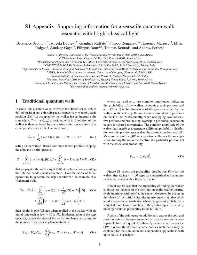
A schematic of the actual experimental setup is given as Fig. S2.Here a pulsed laser (Spectraphysics Quanta-Ray DCR-11) ata wavelength of 1064 nm generated a single input light pulsewith 0 OAM (initial position of the walker). As we did not havean gated detector for this wavelength the laser was frequencyadjusted by second harmonic generation, resulting in the highlosses of the system and hence limiting the maximum number ofsteps possible. To this end a non-linear SHG crystal convertedthe wavelength to 532 nm through frequency doubling to remainwithin the ICCD (iStar AndOR) detection range. This step pro-hibited amplification within the cavity due to the lack of suitablegain media at this wavelength. Structuring a Gaussian intensitydistribution of appropriate beam size was accomplished througha spatial filter which led to significant losses, thus limiting themaximum step number we could achieve. Propagation of thepulse through a HWP served to prepare the input polarizationstate symmetry (e.g., diagonal polarization for a symmetricalHadamard QW), after which, it was injected into the resonator(3 m perimeter) by a 50:50 non-polarizing beam-splitter. Place-ment of the QP (q = 0.5) and WP concatenation initialized theQW and advanced it by one step with each consecutive roundtrip. The output pulse from the beam-splitter was subsequentlyimaged from the QP plane to the mode sorter. Alignment of themode sorter was attained by constructing an adjoining OAMmode generation setup (see Supplementary Information). Herea 532 nm wavelength diode laser was expanded with a 10×objective lens and collimated through an f = 300 mm lens ontoan SLM where phase and amplitude modulation was utilized togenerate superpositions of LG beams. A 4-f system was built toisolate and image the 1st diffraction order onto the mode sorter.The SLM generated mode was then combined and aligned withthe output mode from the resonator with a 50:50 BS. By passingtest OAM superpositions from the SLM through the MS, opti-mal alignment of the elements was then achieved. The Fourierplane of the MS configuration was directed and imaged ontothe ICCD plane with another 4-f system. Choice placement of apopup mirror before the MS and within the FP imaging systemallowed the QP plane image to be re-imaged onto the ICCDwith a lens placed between the pop-up mirrors. The second lensin the MS imaging system then served a dual purpose as the sec-ond imaging lens in the 4-f re-imaging system of the QP plane.This allowed the output beam structure for each pulse to beindividually captured for each round trip, simplifying the align-ment process. Subsequent capture of each round-trip pulse wasachieved through utilization of an iStar AndOR ICCD camerawith a temporal resolution on the 10 ns scale. Synchronizationbetween the initial laser pulse and recording window of thecamera was attained with a Stanford delay generation workingin combination with the iStar on-board digital delay generator.

2.2 The q-plate2.2.1 Action of the q-plate

The q-plate (QP) used in our experiment was a patterned liquidcrystal static element which imparted geometrical phase to thelight field transmitted through. Here the charge (q) of the platedictates the OAM value generated while the polarization of theincoming beam controls the handedness of the OAM generated[2]. It follows that polarization could thus be used as a controlfor the laddering of OAM to higher or lower values in eitherhandedness (positive or negative OAM). Operation of the QP inthe circular polarisation basis is given by the Jones matrix [3, 4]

QP =[

0 ie−i2qφ

iei2qφ 0

](S6)

Incident right circular polarisation (RCP), |R〉 = [1; 0], thengains the phase, ei2qφ, resulting in an OAM of l = 2q~ perphoton. The polarization is subsequently flipped to left circularpolarisation (LCP) in the process. Similarly, LCP, |L〉 = [0; 1],acquires the phase e−i2qφ, resulting in negative OAM of l =−2q~. The i-value multiplying the phase terms is global andthus may be ignored. It follows that the QP operation may becondensed into the following selection rules:

QP |l,R〉 = |l + 2q, L〉 (S7a)

QP |l, L〉 = |l − 2q,R〉 (S7b)

Additionally, this effective twisting of the light beam pro-duced by geometric phase has further implications in the physi-cal interpretation whereby the CP polarization may also be seenin terms of spin angular momentum (SAM). Here when RCPis incident on the QP, OAM of 2q~ per photon is generated,and the flip in CP corresponds to a flip in SAM from 1~ perphoton to −1~. It is well known that transference of SAM andOAM can occur between light and certain matter [4]. Here,SAM interaction occurs in optically anisotropic media such asbirefringent material and OAM in transparent inhomogeneous,isotropic media [2]. The combination of a thin birefringent(liquid crystal) plate with an inhomogeneous optical axis in theQP subsequently results in the element coupling these two formof angular momentum such that flipping in the SAM may beseen to generate OAM, making the QP a spin-to-orbital angu-lar momentum converter (STOC) where the symmetry of theoptical axis patterning effects the conversion values [4].

Characterisation of the q = 0.5 QP used was then carriedout. Figure S3 illustrates the experimental setup implemented toachieve this. A horizontally polarized HeNe laser (wavelength633 nm) was shone through a QWP before being incident on theQP. A polarization grating (PG) was placed before a SpiriconSPU620 camera which acted to spatially separate the left andright CP of the QP generated beam.

Variation of the incoming SAM or CP onto the QP wasobtained by rotating the QWP fast axis. It follows that superpo-sitions of SAM with various weightings was incident onto theQP based on the QWP angle. These input weightings are shownin Fig S4 (a) through projection into RCP and LCP states. The

March 20, 2019 2/19

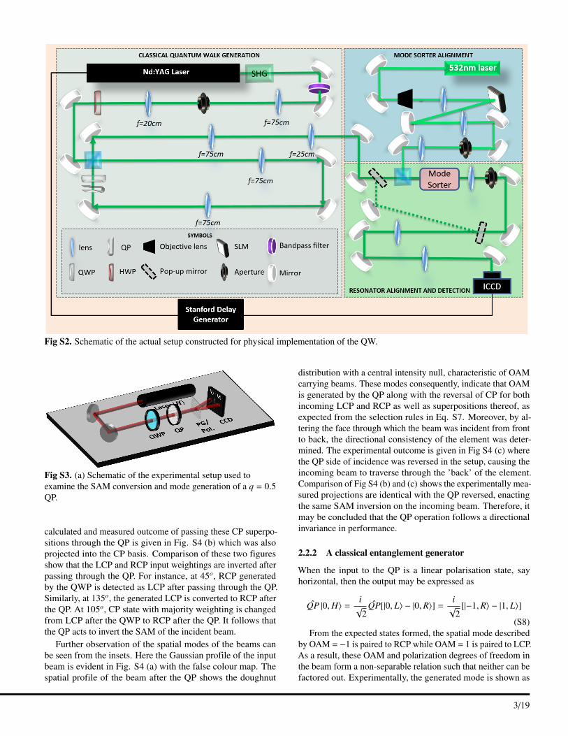
Fig S2. Schematic of the actual setup constructed for physical implementation of the QW.

Fig S3. (a) Schematic of the experimental setup used toexamine the SAM conversion and mode generation of a q = 0.5QP.

calculated and measured outcome of passing these CP superpo-sitions through the QP is given in Fig. S4 (b) which was alsoprojected into the CP basis. Comparison of these two figuresshow that the LCP and RCP input weightings are inverted afterpassing through the QP. For instance, at 45o, RCP generatedby the QWP is detected as LCP after passing through the QP.Similarly, at 135o, the generated LCP is converted to RCP afterthe QP. At 105o, CP state with majority weighting is changedfrom LCP after the QWP to RCP after the QP. It follows thatthe QP acts to invert the SAM of the incident beam.

Further observation of the spatial modes of the beams canbe seen from the insets. Here the Gaussian profile of the inputbeam is evident in Fig. S4 (a) with the false colour map. Thespatial profile of the beam after the QP shows the doughnut

distribution with a central intensity null, characteristic of OAMcarrying beams. These modes consequently, indicate that OAMis generated by the QP along with the reversal of CP for bothincoming LCP and RCP as well as superpositions thereof, asexpected from the selection rules in Eq. S7. Moreover, by al-tering the face through which the beam was incident from frontto back, the directional consistency of the element was deter-mined. The experimental outcome is given in Fig S4 (c) wherethe QP side of incidence was reversed in the setup, causing theincoming beam to traverse through the ’back’ of the element.Comparison of Fig S4 (b) and (c) shows the experimentally mea-sured projections are identical with the QP reversed, enactingthe same SAM inversion on the incoming beam. Therefore, itmay be concluded that the QP operation follows a directionalinvariance in performance.

2.2.2 A classical entanglement generator

When the input to the QP is a linear polarisation state, sayhorizontal, then the output may be expressed as

QP |0,H〉 =i√

2QP[|0, L〉 − |0,R〉] =

i√

2[|−1,R〉 − |1, L〉]

(S8)From the expected states formed, the spatial mode described

by OAM = −1 is paired to RCP while OAM = 1 is paired to LCP.As a result, these OAM and polarization degrees of freedom inthe beam form a non-separable relation such that neither can befactored out. Experimentally, the generated mode is shown as

March 20, 2019 3/19

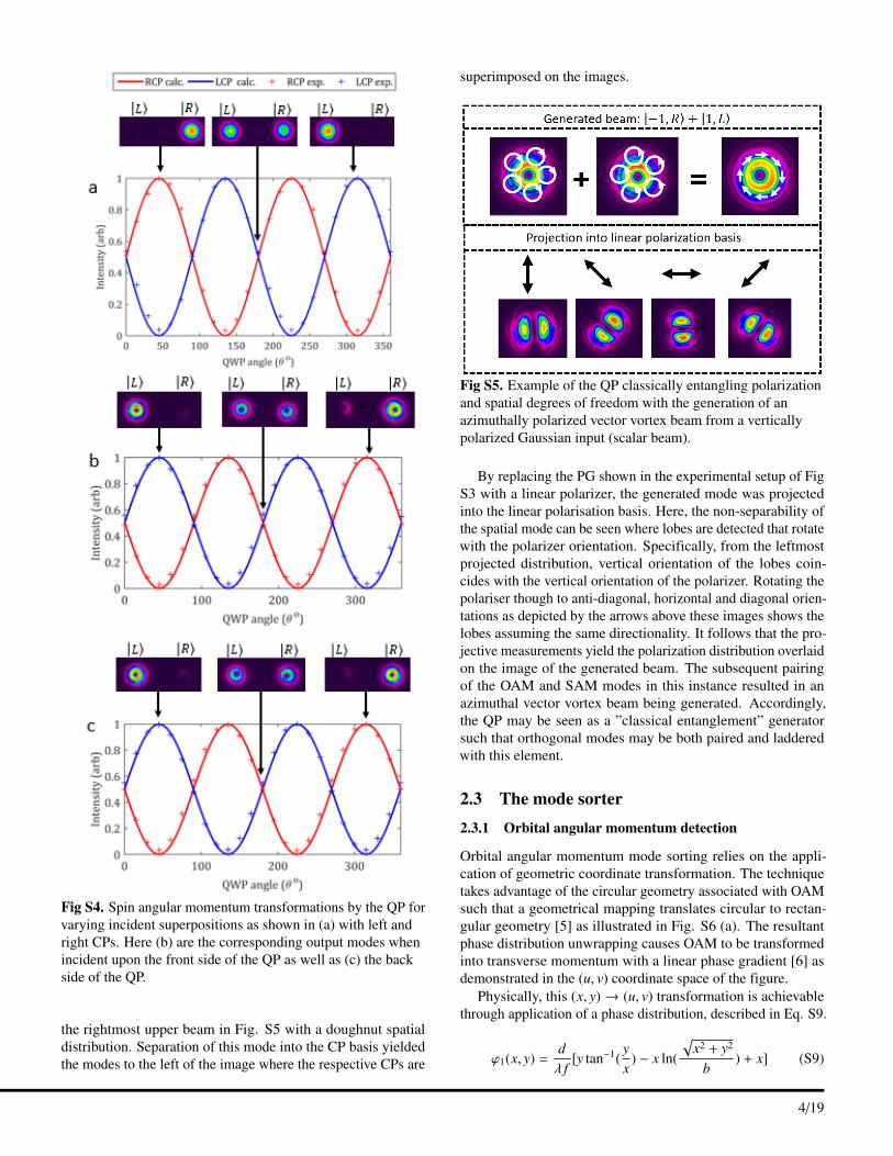
Fig S4. Spin angular momentum transformations by the QP forvarying incident superpositions as shown in (a) with left andright CPs. Here (b) are the corresponding output modes whenincident upon the front side of the QP as well as (c) the backside of the QP.

the rightmost upper beam in Fig. S5 with a doughnut spatialdistribution. Separation of this mode into the CP basis yieldedthe modes to the left of the image where the respective CPs are

superimposed on the images.

Fig S5. Example of the QP classically entangling polarizationand spatial degrees of freedom with the generation of anazimuthally polarized vector vortex beam from a verticallypolarized Gaussian input (scalar beam).

By replacing the PG shown in the experimental setup of FigS3 with a linear polarizer, the generated mode was projectedinto the linear polarisation basis. Here, the non-separability ofthe spatial mode can be seen where lobes are detected that rotatewith the polarizer orientation. Specifically, from the leftmostprojected distribution, vertical orientation of the lobes coin-cides with the vertical orientation of the polarizer. Rotating thepolariser though to anti-diagonal, horizontal and diagonal orien-tations as depicted by the arrows above these images shows thelobes assuming the same directionality. It follows that the pro-jective measurements yield the polarization distribution overlaidon the image of the generated beam. The subsequent pairingof the OAM and SAM modes in this instance resulted in anazimuthal vector vortex beam being generated. Accordingly,the QP may be seen as a ”classical entanglement” generatorsuch that orthogonal modes may be both paired and ladderedwith this element.

2.3 The mode sorter2.3.1 Orbital angular momentum detection

Orbital angular momentum mode sorting relies on the appli-cation of geometric coordinate transformation. The techniquetakes advantage of the circular geometry associated with OAMsuch that a geometrical mapping translates circular to rectan-gular geometry [5] as illustrated in Fig. S6 (a). The resultantphase distribution unwrapping causes OAM to be transformedinto transverse momentum with a linear phase gradient [6] asdemonstrated in the (u, v) coordinate space of the figure.

Physically, this (x, y) → (u, v) transformation is achievablethrough application of a phase distribution, described in Eq. S9.

ϕ1(x, y) =dλ f

[y tan−1(yx

) − x ln(

√x2 + y2

b) + x] (S9)

March 20, 2019 4/19

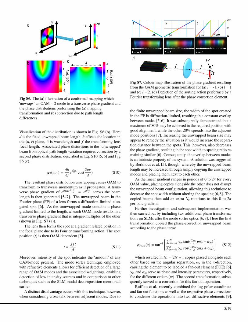
Fig S6. The (a) illustration of a conformal mapping which‘unwraps’ an OAM = 2 mode to a transverse phase gradient andthe phase distributions preforming the (a) mappingtransformation and (b) correction due to path lengthdifferences.

Visualization of the distribution is shown in Fig. S6 (b). Hered is the fixed unwrapped beam length, b affects the location inthe (u, v) plane, λ is wavelength and f the transforming lensfocal length. Associated phase distortions in the ‘unwrapped’beam from optical path length variation requires correction by asecond phase distribution, described in Eq. S10 [5, 6] and FigS6 (c).

ϕ2(u, v) =dbλ f

e−2πu

d cos(2πvd

) (S10)

The resultant phase distribution unwrapping causes OAM totransform to transverse momentum as it propagates. A trans-verse phase gradient of eil tan−1 ( y

x ) = eil 2πvd across the beam

length is then generated [5–7]. The unwrapped beam in theFourier plane (FP) of a lens forms a diffraction-limited elon-gated spot [6]. As the unnwrapped mode contains a phasegradient limited to the length, d, each OAM mode results in atransverse phase gradient that is integer-multiples of the other(shown in Fig. S7 (a)).

The lens then forms the spot at a gradient related position inthe focal plane due to its Fourier transforming action. The spotposition (t) is then OAM-dependent [5].

t =λ f ld

(S11)

Moreover, intensity of the spot indicates the ‘amount’ of anyOAM-mode present. The mode sorter technique employedwith refractive elements allows for efficient detection of a largerange of OAM modes and the associated weightings, enablingdetection of low intensity sources and in comparison to othertechniques such as the SLM modal decomposition mentionedearlier.

A distinct disadvantage occurs with this technique, however,when considering cross-talk between adjacent modes. Due to

Fig S7. Colour map illustration of the phase gradient resultingfrom the OAM geometric transformation for (a) l = -1, (b) l = 1and (c) l = 2. (d) Depiction of the sorting action performed by aFourier transforming lens after the phase correction element.

the finite unwrapped beam size, the width of the spot createdin the FP is diffraction-limited, resulting in a constant overlapbetween modes [5, 6]. It was subsequently demonstrated that amaximum of 80% may be achieved in the required position withgood alignment, while the other 20% spreads into the adjacentmode positions [7]. Increasing the unwrapped beam size mayappear to remedy the situation as it would increase the separa-tion distance between the spots. This, however, also decreasesthe phase gradient, resulting in the spot width to spacing ratio re-maining similar [6]. Consequently, the overlap between modesis an intrinsic property of the system. A solution was suggestedby Berkhout et al. [5], though, whereby the unwrapped beamlength may be increased through simply copying the unwrappedmodes and placing them next to each other.

As the linear gradient ranges in periods of 0 to 2π for everyOAM value, placing copies alongside the other does not disruptthe unwrapped beam configuration, allowing this technique todecrease the spot width without altering the spacing [6, 8]. Thecopied beams then add an extra Nc rotations to this 0 to 2πperiodic gradient.

Further investigation and subsequent implementation wasthen carried out by including two additional phase transforma-tions on SLMs after the mode sorter optics [6, 8]. Here the firsttransformation copied the phase-correction unwrapped beamaccording to the phase term:

ϕFOE(x) = tan−1

∑Nm=−N γm sin(( 2πω

λ)mx + αm)∑N

m=−N γm cos(( 2πωλ

)mx + αm)

(S12)

which resulted in Nc = 2N + 1 copies placed alongside eachother based on the angular separation, ω, in the x-direction,causing the element to be labeled a fan-out element (FOE) [6].γm and αm serve as phase and intensity parameters, respectively,for the different orders (m). The second transformation subse-quently served as a correction for this fan-out operation.

Ruffato et al. recently combined the log-polar coordinateand fan-out functions as well as the respective phase correctionsto condense the operations into two diffractive elements [9].

March 20, 2019 5/19

Fig S8. (a) OAM demultiplexing with log-pol opticaltransformation without and with the integration of a 3-copyoptical fan-out. The generation of multiple copies increases thespatial extent of the linear phase gradient and therefore reducesthe width of the final spots after Fourier transform with a lens.(b) Sorting of OAM beams with log-pol optical transformationin the traditional architecture with the two optical elements insequence: unwrapper (UW) and phase-corrector (PC). Theintegration of a fan-out term producing multiple copies (fan-outunwrapper UW+FO3, double phase-corrector PC3) increasesthe OAM resolution.

Here the copying element was combined with the unwrapperso that the beam could be simultaneously copied Nc times andunwrapped alongside each other before encountering the secondelement [10]. Subsequently, the correction terms for the pathlength difference from the unwrapper is combined with thecorrections for joining the copied beams such that a dual andonce-off correction is carried out on the beam. It follows thatmore accuracy should be expected with this method in additionto the convenience of utilizing a more compact system, wherethe alignment for the system is restricted to half the elementsgiven in the scheme implemented by Mirhosseini et al. [6].

The subsequent working principal behind the elements byRuffato et. al. is depicted in Fig. S8.

2.3.2 Mode sorter performance

To characterize the expected performance in detecting the QW,analysis of both the refractive and diffractive mode sortingelements used in the experiement was carried out. Table S3gives the fabrication parameters of the tested sorters.

The tested diffractive sorters varied in the number of copiesthat were created where 1 and 3 copies were generated respec-tively. As the 1-copy and refractive sorter both generated asingle unwrapped beam, the expected difference in performancebetween the sorters was limited to the range of OAM modes thatcould be accurately sorted. This is due to the refractive sorter

Table S1. Comparison of design parameters for therefractive and diffractive sorters.

Design Parameters RefractiveSorter

DiffractiveSorter

Element diameter (mm) 12.7 2.0Incident beam radius (mm) ≤ 2.10 0.500–0.800Design wavelength (nm) 633 632.8

Wavelength range, λ (nm) 400–1000 532–732

Separation between ele-ments (mm) 300.5 8.500

Unwrapped beam length, d(mm) 10.5 1.12 (1–copy)

0.500(3–copy)

Fig S9. Illustration of the sorting action of a MS (bottom row)for a range of encoded OAM values (top row) between [-3,3].

being able to receive beams of lager radii, thus compensating forthe increased deviation of the angle of incidence for the beamrays directed to the sorter as the OAM increases. A higher rangeof the sorted OAM values being viably accurate [7] should thusoccur. As a result, evaluation of the refractive sorter was re-stricted to the comparative OAM ranges while the 1- and 3-copysorters were further characterized, allowing a more accuratecomparison due to the parameter similarities.

Figure S9 experimentally illustrates the transformation per-formed by the mode sorter on LG modes ranging from -3 to3 OAM. Here the top row shows the modes generated by theSLM and directed through the sorter. The OAM per photon isgiven above the respective spatial modes. In the row below, theelongated spots formed in the FP of the sorting lens are shown.Cross-hairs in the images mark the position of the 0 OAM mode.Consequently, the OAM dependent sorting power of the ele-ments may be clearly seen where the negative OAM spots areformed to the left of the cross-hairs and the positive OAM spotsto the right. Additionally, the position moves incrementally inthe OAM handedness direction, based on the OAM value.

2.3.3 Spot positions

Quantitative evaluation of the spot positions was carried outwhereby experimental measurement of the spots formed forvarying OAM was compared to calculated values determinedfrom Eq. S11. Anticipation of both the accuracy and consistency

March 20, 2019 6/19

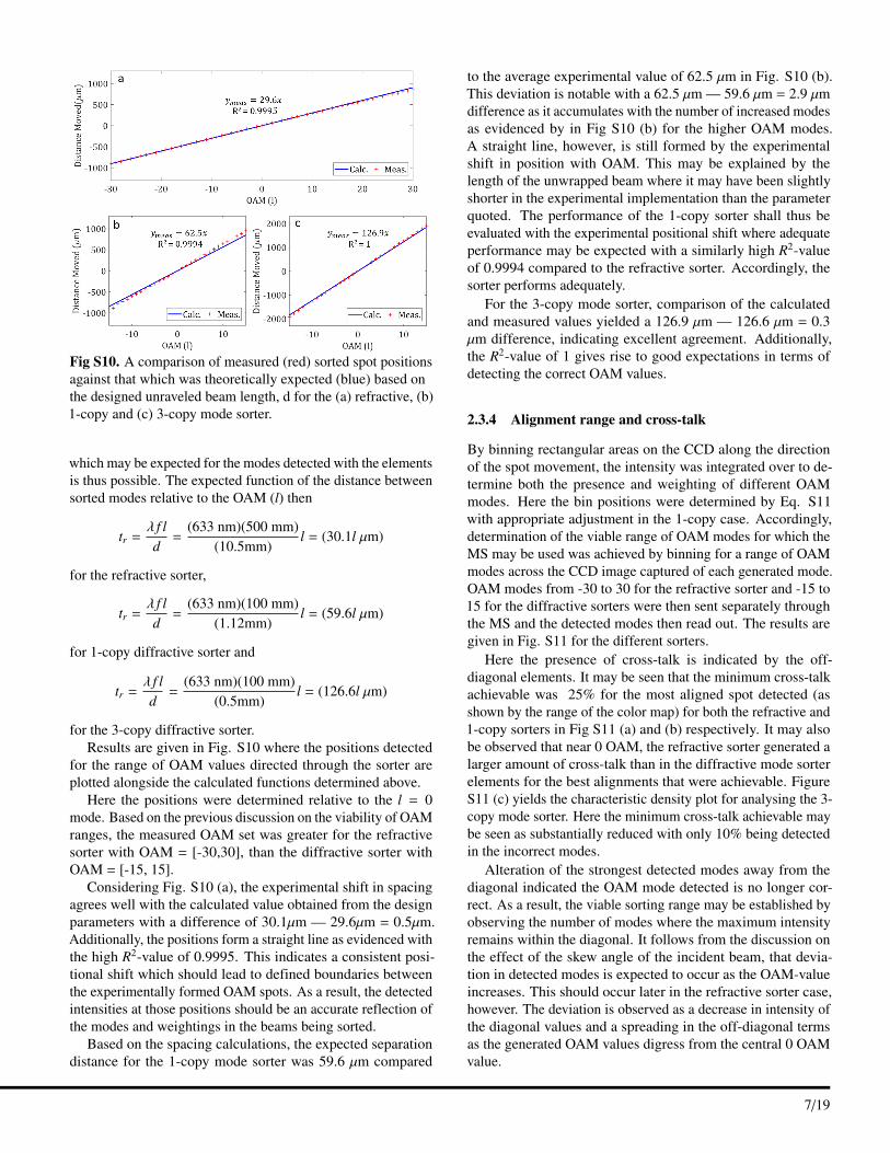
Fig S10. A comparison of measured (red) sorted spot positionsagainst that which was theoretically expected (blue) based onthe designed unraveled beam length, d for the (a) refractive, (b)1-copy and (c) 3-copy mode sorter.

which may be expected for the modes detected with the elementsis thus possible. The expected function of the distance betweensorted modes relative to the OAM (l) then

tr =λ f ld=

(633 nm)(500 mm)(10.5mm)

l = (30.1l µm)

for the refractive sorter,

tr =λ f ld=

(633 nm)(100 mm)(1.12mm)

l = (59.6l µm)

for 1-copy diffractive sorter and

tr =λ f ld=

(633 nm)(100 mm)(0.5mm)

l = (126.6l µm)

for the 3-copy diffractive sorter.Results are given in Fig. S10 where the positions detected

for the range of OAM values directed through the sorter areplotted alongside the calculated functions determined above.

Here the positions were determined relative to the l = 0mode. Based on the previous discussion on the viability of OAMranges, the measured OAM set was greater for the refractivesorter with OAM = [-30,30], than the diffractive sorter withOAM = [-15, 15].

Considering Fig. S10 (a), the experimental shift in spacingagrees well with the calculated value obtained from the designparameters with a difference of 30.1µm — 29.6µm = 0.5µm.Additionally, the positions form a straight line as evidenced withthe high R2-value of 0.9995. This indicates a consistent posi-tional shift which should lead to defined boundaries betweenthe experimentally formed OAM spots. As a result, the detectedintensities at those positions should be an accurate reflection ofthe modes and weightings in the beams being sorted.

Based on the spacing calculations, the expected separationdistance for the 1-copy mode sorter was 59.6 µm compared

to the average experimental value of 62.5 µm in Fig. S10 (b).This deviation is notable with a 62.5 µm — 59.6 µm = 2.9 µmdifference as it accumulates with the number of increased modesas evidenced by in Fig S10 (b) for the higher OAM modes.A straight line, however, is still formed by the experimentalshift in position with OAM. This may be explained by thelength of the unwrapped beam where it may have been slightlyshorter in the experimental implementation than the parameterquoted. The performance of the 1-copy sorter shall thus beevaluated with the experimental positional shift where adequateperformance may be expected with a similarly high R2-valueof 0.9994 compared to the refractive sorter. Accordingly, thesorter performs adequately.

For the 3-copy mode sorter, comparison of the calculatedand measured values yielded a 126.9 µm — 126.6 µm = 0.3µm difference, indicating excellent agreement. Additionally,the R2-value of 1 gives rise to good expectations in terms ofdetecting the correct OAM values.

2.3.4 Alignment range and cross-talk

By binning rectangular areas on the CCD along the directionof the spot movement, the intensity was integrated over to de-termine both the presence and weighting of different OAMmodes. Here the bin positions were determined by Eq. S11with appropriate adjustment in the 1-copy case. Accordingly,determination of the viable range of OAM modes for which theMS may be used was achieved by binning for a range of OAMmodes across the CCD image captured of each generated mode.OAM modes from -30 to 30 for the refractive sorter and -15 to15 for the diffractive sorters were then sent separately throughthe MS and the detected modes then read out. The results aregiven in Fig. S11 for the different sorters.

Here the presence of cross-talk is indicated by the off-diagonal elements. It may be seen that the minimum cross-talkachievable was 25% for the most aligned spot detected (asshown by the range of the color map) for both the refractive and1-copy sorters in Fig S11 (a) and (b) respectively. It may alsobe observed that near 0 OAM, the refractive sorter generated alarger amount of cross-talk than in the diffractive mode sorterelements for the best alignments that were achievable. FigureS11 (c) yields the characteristic density plot for analysing the 3-copy mode sorter. Here the minimum cross-talk achievable maybe seen as substantially reduced with only 10% being detectedin the incorrect modes.

Alteration of the strongest detected modes away from thediagonal indicated the OAM mode detected is no longer cor-rect. As a result, the viable sorting range may be established byobserving the number of modes where the maximum intensityremains within the diagonal. It follows from the discussion onthe effect of the skew angle of the incident beam, that devia-tion in detected modes is expected to occur as the OAM-valueincreases. This should occur later in the refractive sorter case,however. The deviation is observed as a decrease in intensity ofthe diagonal values and a spreading in the off-diagonal termsas the generated OAM values digress from the central 0 OAMvalue.

March 20, 2019 7/19

Fig S11. A density plot showing the sorting power and theassociated cross-talk that may be expected with acceptablealignment for the (a) refractive, (b) 1-copy mode sorter and (c)3-copy mode sorter.

In Fig. S11 (a), the range of modes for which correct OAMmodes are detected is [-20,20] with the refractive sorter. FromFig. S11 (b), with the 1-copy sorter, about 15 modes fall within arange of acceptable accuracy where the intensity that is detectedin the correct mode remains above 60%. A greater range maystill be used for the mode sorter, provided correction terms areused for the non-existent modes being detected as well as lossof weighting in the correctly detected modes. However, this isalso limited as past 20 modes, the defining spot disintegratesinto a fringe array for which the positions are not indicative ofthe modes present.

The range of viable modes with detected weightings greaterthan 60% for the correct mode increased to 23 in the 3-copycase. Additionally, the spread of the cross-talk between modeswas reduced due to the additional number of unwrapped beams.A stronger along-side diagonal may be seen, however, in com-parison to Figure S11 (b). This may be attributed to the greatermisalignment between the elements as the sensitivity of theelement increased with the number of the beams copied. Sub-sequently, additional fringes were caused directly adjacent tothe spot, yielding a stronger presence of erroneous detection ofadjacent OAM modes.

It follows that greater accuracy of the detected modes wasfound with the diffractive sorters, however, the range of OAMmodes were diminished by the small radius of the element. Asa result, the refractive sorter remained consistent over almosttwice the OAM range in comparison to the diffractive elements,illustrating this point for a beam size of 6 mm. Increasing theincoming beam size will subsequently also increase the sortingrange.

2.3.5 Spot resolution

By superimposing sets of alternating OAM spots, the resolutionof adjacent spots were investigated. This was done for the 1-copy sorter in Fig. S12 (a). Here superpositions of even and oddOAM modes in the interval [-7,7] were separately sent throughthe sorter and imaged. Superimposing these modes clearlydescribes how the modes overlap (also seen shown with the 2Dprofiles below the spots). A clear overlap may consequently beseen which will lead to additional cross-talk for the detection ofOAM modes not present.

Fig S12. Images showing resolution for adjacent OAM modeswhen sorted with (a) a 1-copy mode sorter with the alternatingodd and even modes between [-7,7] superimposed along withtheir 2D profiles, (b) adjacent OAM modes between [-1,-8]sorted by the 1-copy mode sorter and (c) adjacent OAM modesbetween [-7,7] sorted by the 3-copy mode sorter.

Additionally, a set of adjacent modes where OAM = [-1,-8]were sent through the mode sorter with the resulting distributionshown in Fig. S12 (b). The convolution resulted in a distortionof the intensity spectrum associated with the OAM present aswell as eliminating the ability to visually distinguish a spot’sposition. The latter may be evidenced through the appearanceof only 6 spot ‘tails’ at the bottom of the convolution when 8OAM modes are present.

The 3-copy mode sorter, however, effectively separated anddefined the spots for adjected OAM modes as is illustrated forFig. S12 (c). Here a superposition of adjacent OAM modes[-7,7] was generated the corresponding detected spots shown inthe figure. A 2D profile is shown below the spots, clearly illus-trating the reduction in overlap and increased spot resolution.

2.3.6 Weighted detection

Accurate detection of mode weightings was also evaluated withthe results given in Fig. S13 (a) and (b) for 1- and 3-copy sortersrespectively. Here a distinct superposition of OAM modes weremultiplexed by the SLM and sent through the sorters.

Comparative accuracy of the multiplexed and detected OAMmodes was determined through its similarity as given by,

S =[∑

l√

Wexp(l)Wth(l)]2∑l Wexp(l)

∑l Wth(l)

(S13)

where Wth(l) is the theoretical or multiplexed weighting associ-ated with the OAM mode l and Wexp(l) is the detected equivalentof the mode. Observation of the Fig. S13 (a) and (b) indicatethat the multiplexed and detected weightings resemble eachother, showing that either of the sorters would be suitable for

March 20, 2019 8/19

Fig S13. Relative weightings evaluated for multiplexed OAMmodes sent through the mode sorter for the (a) 1-copy and (b)3-copy mode sorters with respective similarities of S = 0.791and S = 0.968.

detection, however, a significant increase in the accuracy ofmodal detection occurs as the copy numbers increase. Morespecifically, the similarity of 79.1% for the 1-copy is increasedby 22% when adding 2-copies.

Consequently, both the refractive and diffractive sorters ex-hibited advantages and disadvantages associated with their im-plementation. Specifically, the refractive mode sorter was morerobust, allowing a greater range of beam sizes to be easily sortedas well as maintaining a larger range of OAM values when gen-erating larger input beam sizes. The accuracy associated withmeasuring the weightings associated with a 1-copy sorter, suchas the refractive one, however, is adversely affected with a79.1% accuracy which may be expected if reasonable alignmentis achieved. Here, the 3-copy diffractive sorter is more advan-tageous with a large increase in accuracy with fair alignment.In addition, the cross-talk measured was substantially smallerwith a reduction in the power erroneously detected for incorrectOAM modes. Implementation of this sorter resulted in a highersensitivity to misalignment, resulting in a more difficult detec-tion system as well as a significant restriction of the size of thebeam that can be sorted. Furthermore, variation of beam sizesthat may be sorted is small as only a deviation of 0.300mm ispossible in comparison to the 8mm range achievable in the re-fractive sorter case. Subsequently, for more robust requirements,the refractive sorter was favorable at the expense of the systemaccuracy; conversely, greater accuracy was achieved with the3-copy diffractive sorter at the expense of the range and somestability of the detection system.

3 Experimental considerations anddata analysis

3.1 Beam profile and spatial filteringElimination aberrations and unwanted modes contained in theinitially laser generated beam was necessary through construc-tion of a spatial filter. Figure S14 (a) shows the transverseoutput profile generated by the Spectraphysics DCR-11 laser.From the transverse distribution, the presence of aberrations andadditional modes are evident in addition to a large beam widthof 3 mm. A spatial filter was implemented with a 50 µm pinholeplaced in the Fourier plane of the 4− f system with lenses of fo-cal lengths, f 1 = 750 mm and f 2 = 200 mm respectively. Here

the pinhole was three times larger than the calculated Gaussianbeam width in the FP, resulting in the extraneous modes beingfiltered out spatially. The focal length ratio ( f 2/ f 1) betweenthe lenses additionally formed a demagnification telescope toreduce the beam diammeter to 2 mm.

Fig S14. False color map images of the near-field pulsed laseroutput beam (a) before spatial filtering and (b) after spatialfiltering. The spatially filtered beam is smaller than the originalas it was de-magnified in the spatial filtering process.

The spatial filter output beam is given in Fig. S14 (b) where aGaussian intensity distribution can be seen along with the appro-priate demagnification. In addition, the reduced size allowed fora more sustainable walk with the dimensions remaining belowthe size of the optics.

3.2 Pulse overlap and adjusting the predictionThe time gap (t) between each output pulse from the resonatoris related to the length of the resonator (L) through the rela-tion, t = L/c where c refers to the speed of light in air and tthe time. Here, the resonator must be longer or equal to thetemporal pulse width to avoid overlap of the circulating pulseand thus an overlap in the QW steps. However, experimentalconsideration as well as stability and alignment factors resultedin an upper limit restriction of 3 m for the resonator perime-ter. It was subsequently designed in a 0.3m × 1.7m rectangularconfiguration.

Measurement of the subsequent temporal pulse width of thelaser was carried out by placing a Thorlabs DET210-a photodi-ode before the ICCD and averaging over 10 intensity pulses ona Tektronix TDS2024B 1GHz oscilloscope. The correspondingtemporal parameters were then estimated by fitting the pulse toa Gaussian function of the form:

G(x) = ae−(x−b)2/(2c2) + k, (S14)

where a determines the height of the pulse function, x refers tothe x-axis position which is then adjusted by b. c indicates thewidth of the pulse and k adjusts the position along the y-axis.The corresponding parameters extracted from fitting Eq. S14are summarized in Table S2 A SSE (sum of the squares of theerror) of 0.002573 and R-squared value of 0.974 determinedfrom the fitting both indicate that the function as well as theparameters are adequate reflections of the measured pulse forthe walker.Here the parameters may subsequently be used to yield boththe mathematical description of the pulse as well as indicate

March 20, 2019 9/19

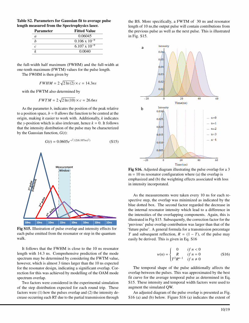
Table S2. Parameters for Gaussian fit to average pulselength measured from the Spectrophysics laser.

Parameter Fitted Valuea 0.06045b 0.106 x 10−9

c 6.107 x 10−9

k 0.0040

the full-width half maximum (FWHM) and the full-width atone-tenth maximum (FWTM) values for the pulse length.

The FWHM is then given by

FWHM = 2√

2 ln (2) × c = 14.3ns

with the FWTM also determined by

FWT M = 2√

2 ln (10) × c = 26.6ns

As the parameter b, indicates the position of the peak relativeto a position space, b = 0 allows the function to be centred at theorigin, making it easier to work with. Additionally, k indicatesthe y-position which is also irrelevant, hence k = 0. It followsthat the intensity distribution of the pulse may be characterizedby the Gaussian function, G(t):

G(t) = 0.0605e−t2/(2(6.107ns)2) (S15)

Fig S15. Illustration of pulse overlap and intensity effects foreach pulse emitted from the resonator or step in the quantumwalk.

It follows that the FWHM is close to the 10 ns resonatorlength with 14.3 ns. Comprehensive prediction of the modespectrum may be determined by considering the FWTM value,however, which is almost 3 times larger than the 10 ns expectedfor the resonator design, indicating a significant overlap. Cor-rection for this was achieved by modelling of the OAM modespectrum overlap.

Two factors were considered in the experimental simulationof the step distribution expected for each round trip. Thesefactors were (1) how the pulses overlap and (2) the intensity de-crease occurring each RT due to the partial transmission through

the BS. More specifically, a FWTM of 30 ns and resonatorlength of 10 ns,the output pulse will contain contributions fromthe previous pulse as well as the next pulse. This is illustratedin Fig. S15.

Fig S16. Adjusted diagram illustrating the pulse overlap for a 3m = 10 ns resonator configuration where (a) the overlap isemphasized and (b) the weighting effects associated with lossin intensity incorporated.

As the measurements were taken every 10 ns for each re-spective step, the overlap was minimized as indicated by theblue dotted box. The second factor regarded the decrease inthe internal resonator intensity which lead to a difference inthe intensities of the overlapping components. Again, this isillustrated in Fig S15. Subsequently, the correction factor for the‘previous’ pulse overlap contribution was larger than that of the‘future pulse’. A general formula for a transmission percentageT and subsequent reflection, R = (1 − T ), of the pulse mayeasily be derived. This is given in Eq. S16

w(n) =

0 i f n < 0R i f n = 0

T 2Rn−1 i f n , 0(S16)

The temporal shape of the pulse additionally affects theoverlap between the pulses. This was approximated by the bestfit curve for the average temporal pulse as determined in Eq.S15. These intensity and temporal width factors were used toaugment the simulated QW.

An adjusted diagram of the pulse overlap is presented as Fig.S16 (a) and (b) below. Figure S16 (a) indicates the extent of

March 20, 2019 10/19

the pulse overlap while (b) illustrates the effects of the differentweightings for a 50 : 50 beamsplitter.

The dotted lines indicate the section of the pulse that wasgated by the AndOR camera for the nth step in the quantumwalk series. This gated section of the pulse was determinedusing the formula:

a =PW −GW

2(S17)

where PW is the complete pulse width (40 ns based on themodelled pulse) and GW is the gate width (i.e. the time sectionof pulse captured).Based on the AndOR gating time, the pulsewas captured from

−PW2+ a = −20 + (

40 − 102

) = −5

toPW2− a = 20 − (

40 − 102

) = 5.

Correction to the quantum walk probability distribution for the1st pulse (n = 0) was thus:

n = 0:

[[QWP(0)]w(0)∫ PW

2 −a

−PW2 +a

G(t)dt]

+ [[QWP(1)]w(1)∫ −PW

2 +a

−PW2 +a−10

G(t)dt]

+ [[QWP(2)]w(2)∫ −PW

2 +a−10

−PW2 +a−20

G(t)dt]

Similarly, for n = 1 and 2:

n = 1:

[[QWP(0)]w(0)∫ PW

2 −a+10

PW2 −a

G(t)dt]

+ [[QWP(1)]w(1)∫ PW

2 −a

−PW2 +a

G(t)dt]

+ [[QWP(2)]w(2)∫ −PW

2 +a

−PW2 +a−10

G(t)dt]

+ [[QWP(3)]w(3)∫ −PW

2 +a−10

−PW2 +a−20

G(t)dt]

n = 2:

[[QWP(0)]w(0)∫ PW

2 −a+20

PW2 −a+10

G(t)dt]

+ [[QWP(1)]w(1)∫ PW

2 −a+10

PW2 −a

G(t)dt]

+ [[QWP(2)]w(2)∫ PW

2 −a

−PW2 +a

G(t)dt]

+ [[QWP(3)]w(3)∫ −PW

2 +a

−PW2 +a−10

G(t)dt]

+ [[QWP(4)]w(4)∫ −PW

2 +a−10

−PW2 +a−20

G(t)dt]

Accordingly, the following general model applies:

n:

[[QWP(n − 2)]w(n − 2)∫ PW

2 −a+20

PW2 −a+10

G(t)dt]

+ [[QWP(n − 1)]w(n − 1)∫ PW

2 −a+10

PW2 −a

G(t)dt]

[[QWP(n)]w(n)∫ PW

2 −a

−PW2 +a

G(t)dt]

+ [[QWP(n + 1)]w(n + 1)∫ −PW

2 +a

−PW2 +a−10

G(t)dt]

+ [[QWP(n + 2)]w(n + 2)∫ −PW

2 +a−10

−PW2 +a−20

G(t)dt] (S18)

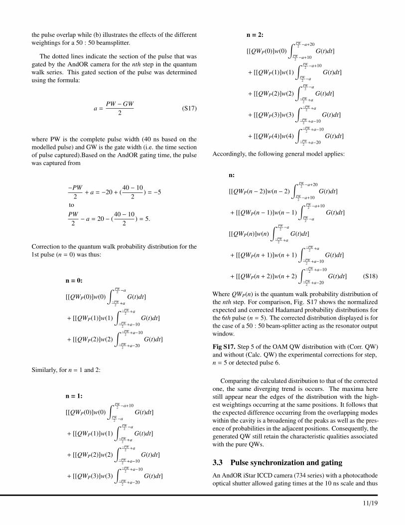
Where QWP(n) is the quantum walk probability distribution ofthe nth step. For comparison, Fig. S17 shows the normalizedexpected and corrected Hadamard probability distributions forthe 6th pulse (n = 5). The corrected distribution displayed is forthe case of a 50 : 50 beam-splitter acting as the resonator outputwindow.

Fig S17. Step 5 of the OAM QW distribution with (Corr. QW)and without (Calc. QW) the experimental corrections for step,n = 5 or detected pulse 6.

Comparing the calculated distribution to that of the correctedone, the same diverging trend is occurs. The maxima herestill appear near the edges of the distribution with the high-est weightings occurring at the same positions. It follows thatthe expected difference occurring from the overlapping modeswithin the cavity is a broadening of the peaks as well as the pres-ence of probabilities in the adjacent positions. Consequently, thegenerated QW still retain the characteristic qualities associatedwith the pure QWs.

3.3 Pulse synchronization and gatingAn AndOR iStar ICCD camera (734 series) with a photocathodeoptical shutter allowed gating times at the 10 ns scale and thus

March 20, 2019 11/19

isolation of the correct round tip. The opening and closing ofthe photocathode was determined by monitoring the electronicsignals, sent to enact the operation in the camera, with an oscil-loscope. As indicated in Fig. S18, the opening is determinedwith a negative pulse and closing with a positive pulse.

Fig S18. Schematic illustrating the procedure necessary tocorrectly capture an output pulse for a single step or round tripin the quantum walk.

The camera and laser pulse emission was synchronised witha digital delay generator so as to locate the desired output pulse(step). A specific time delay was then placed between the pulseemission and opening of the photocathode. The delay chosenwas equivalent to the time taken for the electronic signals totravel to the respective components as well as the time for thepulse to reach the resonator, circulate the resonator a desirednumber of times, travel through the sorter and reach the camera.To determine the delay, a photodiode was placed at the samedistance from the output as the camera. Arrival of the pulse oncefired triggered the oscilloscope which was also monitoring thephotocathode trigger signal in a second channel. Adjustment ofthe calculated time delay altered the first detected pulse (step 0)temporal position as depicted in Fig. S19. After determinationof the initial pulse delay, isolation of the desired step or pulseoutput was achieved by adding an additional delay of Nt that isrelated to the resonator circulation time, t and number of steps,N.

Determination of the appropriate delay required for synchro-nization of the camera and laser pulse is demonstrated in Fig.S19. The graphs along the lower row of the figure are signalsrecorded by a oscilloscope monitoring the photocathode trig-gering signals as well as the arrival of the emitted laser pulsedue to a trigger pulse from the digital delay generator for thesame nanosecond time scale (x-axis). The y-axis then representsthe associated voltages. It follows that the blue profile is thelaser pulse detected by the photodiode, placed the same distanceas the camera from the output pulse and the red profile is thetrigger signals operating the opening (first large dip) and closing(first large spike) of the photocathode. Transparent green over-lays on the respective graphs emphasize the period for whichthe camera is recording the pulse intensity and thus the sectionof the pulse captured. As indicated, the gate width (capturing

Fig S19. Experimental illustration of synchronization requiredbetween the AndOR camera and pulsed laser for accurateoutput pulse capture from the QW resonator. Delay timesettings were decreased from (a-d).

time) was set to 10 ns.Images above each of the oscilloscope graphs are the trans-

verse intensity distributions captured in the respective 10 nsgated windows where the delay between the photocathode andlaser triggers from the digital delay generator was systematicallydecreased from (a) through to (b) for a three-lobe spatial profile.It can thus be seen from (a)-(b) how the pulse moves into thecapturing window of the camera before the maximum pulseintensity is captured in (c) and then moving past the range againin (d). The variation in intensity of the captured modes clearlyshow the synchronization effects of the time delay parameterand the desired position for ideal analysis of an output pulsewith (c).

Application of the appropriate synchronization time delayas determined with the method illustrated in Fig. S19 for thefirst pulse in the resonator setup is allowed for the capture of thedesired QW step or output pulse. Subsequent addition of a step-related time delay constant, Nt, to the initial delay allowed forthe capture of the intensity distribution related to that step (N) oroutput pulse. This is illustrated in Fig. S20 for the experimentalsetup. Here successive output pulse intensity distributions fromN = [0, 4] were captured with a 10 ns gate width in the modesorter Fourier plane. A clear evolution in the distribution maybe seen across the steps, indicating a spread in the intensitydistribution and thus the successful capture of additional outputpulses according to the associated delay settings. It follows thatthis method would be effective in attaining the OAM spectra ofeach QW step, allowing real-time observation of the walk.

3.4 Experimental data correctionFollowing the noted overlap occurring in the experimental setupand the associated derivation of the correction to the theory,the measured experimental results were expected to have anadjusted distribution as indicted by Eq. S18. Accordingly, thesimulated distribution was altered as illustrated by Fig. S17.Comparison between the directly measured experimental distri-bution and altered theory thus allowed the QW distribution toevaluated. The results in this form are shown by the gray bargraphs (to the left) in Fig. S21 for the symmetric HadamardQW case, Fig. S22 for the asymmetric Hadamard QW, Fig. S23

March 20, 2019 12/19

Fig S20. Example evolution of output intensity distributions ascaptured every consecutive 10ns from the first output pulse,marking each round trip made by the circulating light beam forthe QW resonator.

where the QW symmetry was changed with the QWP fast axisorientation, Fig. S24 for the Identity coin QW and Fig. S25 forthe NOT-coin QW.

However, in order appropriately evaluate the QW distribu-tions with respect to what is traditionally expected, it was alsopossible to reverse the overlap and correct the measured distri-bution such that it reflected the characteristic QW commonlyseen. This was accomplished by taking the QW distributionmeasured for the nth step and applying the reverse of Eq. S18such that the QWP(n)meas could be retrieved or de-convolutedfrom the measured distribution.

To generate the experimental correction, consider simplify-ing the equation by simplifying the terms specified in Table S3by the variables listed.

Table S3. Equation S18 term simplification.Variable Equation termc(n−2) w(n − 2)

∫ PW2 −a+20

PW2 −a+10

G(t)dt]

c(n−1) w(n − 1)∫ PW

2 −a+10PW2 −a

G(t)dt]

cn w(n)∫ PW

2 −a−PW

2 +aG(t)dt]

c(n+1) w(n + 1)∫ −PW

2 +a−PW

2 +a−10G(t)dt]

c(n+2) w(n + 2)∫ −PW

2 +a−10−PW

2 +a−20G(t)dt]

Equation S18 then becomes

QWPCorr(n) =c(n−2)QWP(n − 2) + c(n−1)QWP(n − 1)+ cnQWP(n) + c(n+1)QWP(n + 1)+ c(n+2)QWP(n + 2), (S19)

where QWPCorr(n) is the probability distribution measured forthe nth step as a result of the overlapping pulses in the resonator.

Now in order to correlate the measured distribution to theexpected, they should both be normalized by dividing the dis-tribution by the sum i.e. S =

∑QWPCorr(n) and S Exp =∑

QWP(n)meas. Letting QWP(n)NORMmeas = QWP(n)meas/S Exp,it follows that

QWP(n)NORMmeas =[c(n−2)QWP(n − 2) + c(n−1)QWP(n − 1)

+ cnQWP(n) + c(n+1)QWP(n + 1)

+ c(n+2)QWP(n + 2)]]÷ S . (S20)

As we are now modifying the experimentally measured data,it follows that QWP(n) is becomes the corrected experimentaldata. Subequently,

QWP(n)meas =QWP(n)NORMmeas × S

cn−[

c(n−2)QWP(n − 2) + c(n−1)QWP(n − 1)

+ c(n+1)QWP(n + 1) + c(n+2)QWP(n + 2)]]÷ cn.

(S21)

After applying the correction, any miscellaneous negativevalues were taken as background errors and equated to 0 as anegative probability is not physically possible. The resulting dis-tributions were then normalized and are respectively presentedin the inset graphs to the right in Fig. S21 to Fig. S25. Herethe blue bars indicate the traditional distributions expected forthese types of QWs and no overlap adjustment is shown. Thismay be clearly seen by where the uncorrected measured valuesoccupy adjacent OAM states or positions while the correctedresults shown occupy alternate OAM states or positions. Thedouble sided arrows in each case indicate the interchangeablecorrections between the simulated and measured probabilitydistributions and the subsequent matching correlations betweenthe experimental and simulated distributions.

March 20, 2019 13/19

Fig S21. Illustration of the results presented in the paper for the symmetrical Hadamard QW with a simulated density plot indicatingthe traditional spread in distribution with a logarithmic color scale over 100 steps. Inset graphs below indicate correlation of theresults where the theory was corrected for overlap (left) vs. where the experimental results were corrected for the overlapping pulses(right). Black lines (color bars) indicate the experimental (simulated) results for (i) Step 1, (ii) Step 6 and (iii) Step 8. The dotted lineindicates the analogous Random walk distribution expected in the classical case for the last step.

March 20, 2019 14/19

Fig S22. Illustration of the results presented in the paper for the asymmetrical Hadamard QW with a simulated density plot indicatingthe traditional spread in distribution with a logarithmic color scale over 100 steps. Inset graphs below indicate correlation of theresults where the theory was corrected for overlap (left) vs. where the experimental results were corrected for the overlapping pulses(right). Black lines (color bars) indicate the experimental (simulated) results for (i) Step 1, (ii) Step 4 and (iii) Step 5. The dotted lineindicates the analogous Random walk distribution expected in the classical case for the last step.

March 20, 2019 15/19

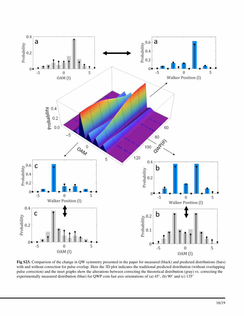
Fig S23. Comparison of the change in QW symmetry presented in the paper for measured (black) and predicted distributions (bars)with and without correction for pulse overlap. Here the 3D plot indicates the traditional predicted distribution (without overlappingpulse correction) and the inset graphs show the alterations between correcting the theoretical distribution (gray) vs. correcting theexperimentally measured distribution (blue) for QWP coin fast axis orientations of (a) 45◦, (b) 90◦ and (c) 135◦

March 20, 2019 16/19

Fig S24. Illustration of the results presented in the paper for the Identity coin QW with a simulated 3D plot indicating the traditionalspread in distribution (left) and adjusted spread (right) due to pulse overlap. Inset graphs below indicate correlation of the resultswhere the theory was corrected for overlap (left) vs. where the experimental results were corrected for the overlapping pulses (right).Black lines (color bars) indicate the experimental (simulated) results for (i) Step 0, (ii) Step 3 and (iii) Step 4.

March 20, 2019 17/19

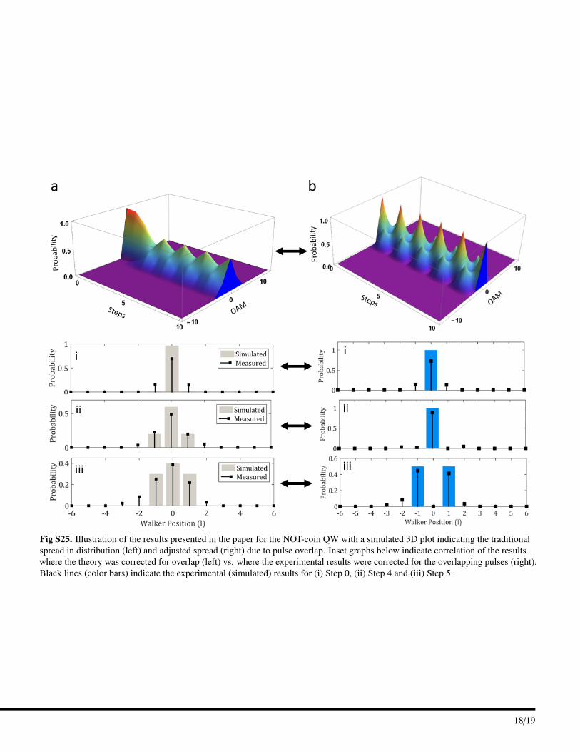
Fig S25. Illustration of the results presented in the paper for the NOT-coin QW with a simulated 3D plot indicating the traditionalspread in distribution (left) and adjusted spread (right) due to pulse overlap. Inset graphs below indicate correlation of the resultswhere the theory was corrected for overlap (left) vs. where the experimental results were corrected for the overlapping pulses (right).Black lines (color bars) indicate the experimental (simulated) results for (i) Step 0, (ii) Step 4 and (iii) Step 5.

March 20, 2019 18/19

References1. Kempe J. Quantum random walks: an introductory

overview. Contemporary Physics. 2003;44(4):307–327.

2. Marrucci L, Manzo C, Paparo D. Optical spin-to-orbital angular momentum conversion in inhomoge-neous anisotropic media. Physical review letters.2006;96(16):163905.

3. Marrucci L, Karimi E, Slussarenko S, Piccirillo B, San-tamato E, Nagali E, et al. Spin-to-Orbital Optical Angu-lar Momentum Conversion in Liquid Crystal “q-Plates”:Classical and Quantum Applications. Molecular Crystalsand Liquid Crystals. 2012;561(1):48–56.

4. Piccirillo B, Slussarenko S, Marrucci L, Santamato E.The orbital angular momentum of light: genesis andevolution of the concept and of the associated photonictechnology. Riv Nuovo Cimento. 2013;36(11):501–555.

5. Berkhout GC, Lavery MP, Courtial J, BeijersbergenMW, Padgett MJ. Efficient sorting of orbital angu-lar momentum states of light. Physical review letters.2010;105(15):153601.

6. Mirhosseini M, Malik M, Shi Z, Boyd RW. Efficientseparation of the orbital angular momentum eigenstatesof light. Nature communications. 2013;4:2781.

7. Lavery MP, Robertson DJ, Sponselli A, Courtial J, Stein-hoff NK, Tyler GA, et al. Efficient measurement ofan optical orbital-angular-momentum spectrum com-prising more than 50 states. New Journal of Physics.2013;15(1):013024.

8. O’Sullivan MN, Mirhosseini M, Malik M, Boyd RW.Near-perfect sorting of orbital angular momentumand angular position states of light. Optics Express.2012;20(22):24444–24449.

9. Ruffato G, Massari M, Parisi G, Romanato F. Test ofmode-division multiplexing and demultiplexing in free-space with diffractive transformation optics. Optics ex-press. 2017;25(7):7859–7868.

10. Ruffato G, Brasselet E, Massari M, Romanato F.Electrically activated spin-controlled orbital angularmomentum multiplexer. Applied Physics Letters.2018;113(1):011109.

March 20, 2019 19/19