s t i t u e - welcome to caltechthesis - caltechthesis · tbak er platform break outs are nearly...
TRANSCRIPT

The State of Stress as Inferred from Deviated Boreholes
Constraints on the Tectonics of Oshore Central California
and Cook Inlet Alaska
Thesis by
Blair J Zajac Jr
In Partial Fulllment of the Requirements
for the Degree of
Doctor of Philosophy
1 8 9 1
CA
LIF
OR
NIA
I
NS T IT U T E O F T
EC
HN
OL
OG
Y
Caltech
Pasadena California
Submitted May

ii
Portions published as Zajac B J and J M Stock J Geophys Res B and
copyright c by the American Geophysical Union
Remaining portions copyright c by Blair J Zajac Jr All Rights Reserved

iii
Acknowledgements
If I was to acknowledge everyone who contributed to the completion of this work it would take as
long as it took to write the thesis Up front I want to apologize to anyone omitted here the time
is to blame the memories pass To all those who contributed my most profound appreciation
First and foremost I want to acknowledge two people whose love support and belief in me made
this dream possible my Mom and Dad Barbara and Blair Zajac I am eternally grateful to them
And to my brother Bard thanks for patiently listening to my complaining and for your love and
support
To Ashley my life partner without whose loving support I would have never completed this task
my everlasting gratitude She prodded me on when I needed it adding her unique touch of nesse
to keep the project moving She has opened my heart to a world of love passion and commitment
I never knew I bless every day that I am with her
Thanks to Joann Stock my advisor who through patience professionalism and academic exper
tise guided me through this journey allowing me to develop my own scientic interests to pursue
them and integrate them in this body of work I thank Rob Clayton who always kept me on course
when things got rough I acknowledge the charming Tom Ahrens who irked me by constantly asking
more from me than I wanted to deliver
My profound gratitude goes to my fellow collaborator Julie Shemeta who worked with me on
the initial development of this work I greatly appreciate Melita Wilde and Martha Kuykendalls
work They digitized my paper well logs saved my back from a tedious job
My thanks go to Mitch Edwards and Pericles Rellas for their diligent support and phone calls
and to Karin Bellomy for her patience To my fellow cohorts at Caltech who made my stay bearable
Hong Kie Thio David Wald and Bruce Worden my thanks And to all of those who persuaded
me to stay and not give up Petr Pich and Don Baneld my thanks To those who did not have a
direct connection with my thesis such as Richard Fagen Cheryl Contopulos Jean Grinols and Jim
Bys I express my thanks for their generosities My thanks goes to Ann Freemen the den mother of
the Seismo Lab whose care and concern brought warmth to a busy place My nal thanks goes to
Landmark Education Corporation where I learned that anything is possible when one is committed

iv
Abstract
This thesis introduces a new method of constraining the vector directions of the three principal
stresses and their relative magnitudes by using borehole breakouts in nonvertical drill holes Unlike
older stress state measurements from breakouts this work does not presume that one of the principal
stresses is vertical This method has important uses in complicated threedimensional structures
such as in the Los Angeles basin and in oil drilling applications
Chapter discusses why knowledge of the threedimensional stress tensor is relevant to todays
science and examines the applications of the stress state determination technique discussed herein
The history of previous work is also described
In Chapter I discuss the techniques of determining the stress tensor from borehole breakouts
examining the physics of borehole breakouts the theory of the inversion technique used and data
processing issues The theory and data processing issues are not discussed separately in this work
since data processing issues often prompted new theoretical techniques I rst examine the physics
of borehole breakouts and how the orientation of breakouts on the borehole wall relates to the local
stress eld A new borehole breakout selection scheme which takes into account highly nonvertical
boreholes is then presented along with a discussion of the real world problems of data gathering
identication and processing Having selected a borehole breakout data set using the criteria I
invert for the best tting stress state using a new technique combining genetic algorithms and non
di erential function optimizers Finally I present a way in which condence limits can be
placed on the resulting stress tensor
With all of the technical and theoretical pieces in place I now examine several di erent data sets
Chapter examines a borehole breakout data set publish by Qian and Pedersen from the
Siljan Deep Drilling Project in Sweden and demonstrates that even for simple borehole breakout data
sets the stress state inversions assuming a vertical principal stress direction may fall outside of the
condence limits of an inversion allowing nonvertical principal stress directions My technique
of displaying the borehole breakout data makes the data quality more obvious as compared to the
way Qian and Pedersen plotted the data
Chapter examines a borehole breakout data set from the o shore Santa Maria Basin California
This analysis presents vertical borehole breakout data that represent a maximum horizontal principal
stress direction of NE roughly consistent with other earthquake focal mechanism GPS and
borehole breakout studies in the area However the stress state inversion of breakouts identied in
the vertical and a limited number of nearly horizontal boreholes suggests a stress state very di erent

v
from any other stress state results This could imply that the three dimensional stress in the Santa
Maria Basin is very complicated However given the limited amount of borehole breakouts identied
in nearly horizontal wells the stress state results from this data set are inconclusive
Chapter examines the largest data set used in this study from a series of oil wells in Cook
Inlet Alaska These are borehole caliper arm data from di erent wells reaching a maximum
deviation of and m true vertical depth Stress state inversions of di erent subsets of
the borehole breakout data were performed Inversion of breakouts identied in the top two of three
marker beds analyzed in wells drilled from the Baker platform identied nearly degenerate thrust
faulting stress states with the maximum principal stress axis S oriented horizontally WNW
ESE perpendicular to the NNEtrending anticlinal structures The stress state from the deepest
marker is also a nearly degenerate thrust faulting stress state with S oriented NNWSSE aligned
with the regional direction of relative plate motion between the North American and Pacic plates
In between the shallow and deep stress state is an apparent normal faulting stress state with S
oriented subhorizontally ENEWSW This clockwise rotation of the stress tensor as a function of
depth suggests that the stress eld changes with depth from a shallow stress state responsible for
the local NNEtrending structures to a deeper one from the North American and Pacic plates
collision zone The observed normal faulting stress state between the two thrust faulting stress
states is anomalous and may represent some sort of transition from the shallow to the deep stress
state Stress state proles in m true vertical depth TVD intervals show consistently oriented
thrust faulting stress regimes with NNWSSE trending S azimuths The thrust faulting S principal
stress direction is consistently within of vertical suggesting that while the assumption of a purely
vertical principal stress direction is not valid the stress tensor does not signicantly rotate away
from the surface conditions that require a purely vertical stress tensor The nearly degenerate thrust
faulting stress states determined from the Granite Point and the km distant Baker platform
breakouts are nearly identical implying that the technique of using deviated borehole breakouts to
invert for the regional stress is valid The orientations of the maximum horizontal stress determined
from the Cook Inlet borehole breakouts are consistent with other stress indicators in southcentral
Alaska and consistent with the direction of relative plate motion between the North American Plate
and the Pacic plate The S axis for the Cook Inlet eld trends due south plunging The
condence limits allow the S azimuth to vary from NE to NE and the plunge to vary from
to This stress state does not appear representative of the stress eld for each subset of
breakouts The Granite Point S axis trends NW plunging the condence limits allow
the azimuth to vary from NW to NE and the plunge to vary from to The Baker platform
S axis trends NE plunging the condence limits on S allow its azimuth to vary from
NE to NE and its plunge to vary from to Finally the Dillon platform S axis trends
NW plunging the condence limits constrain the S azimuth from NE to NE

vi
and the plunge from to The more westerly orientation of S at the Dillon platform may be
related to the local NNEtrending anticlinal structures in the Cook Inlet Basin
Chapter concludes and summarized the results and conclusions from the thesis
The rst appendix contains in minute detail some of the mathematics describing the boreholes
breakouts and coordinate system rotations used to perform this work The second appendix contains
the individual discussion and plots of the raw dipmeter data from all of the Cook Inlet Alaska wells

vii
Contents
Acknowledgements iii
Abstract iv
Introduction
Objective and Motivation
Overview of Thesis
Borehole Breakout Data Gathering Processing and Inverting
Mathematical and Physical Description of Boreholes and Data Processing
Dening the Borehole and Geographic Coordinate Systems
Data Collection from Well Logs Well Log Measurements
Calculation of Elongation IJK Angles
Calculation of Borehole and Elongation XYZ Azimuths
Statistics of Angular Data
Identication of Breakouts
Propagation of Errors
Inverting the Breakout Data
Binning of Breakout Data
Euler Angle Description of a Stress State
Theoretical Breakout Directions in Arbitrary Stress Fields
Selection and Calculation of a Mist Measure
Fitting the Breakout Data
Condence Limits
Condence Limits on Individual Stress State Parameters
Analysis of the Siljan Deep Drilling Project Breakout Data
Analysis of the Point Pedernales Data
The Stress State and Its Depth Dependence in Cook Inlet Alaska
Abstract
Introduction

viii
Geology and Stratigraphy of the Cook Inlet Basin
Data Description and Processing
O shore Oil Platforms and Summary of Raw Data
Well Log Processing
Borehole Breakout Selection
Selection of Borehole Breakout Data Subsets
Individual Discussion of Wells
Inversion of Borehole Breakouts
Stress State Analyses
Granite Point Oil Field Inversion
Baker Platform Inversion
Dillon Platform Inversion
Cook Inlet Inversion
Results and Conclusions
Overview of Results
Regional Stress State
Conclusions
A Detailed Mathematical Derivations
A Derivation of the Rotation Matrices
A Checking the Rotation Matrices
A Construction and Rotation of the Downgoing Borehole Axis Vector
A Construction and Rotation of the I Axis
A Construction and Rotation of the J Axis
A Transformations of Stress Tensors between Frames
A Transforming Angles between the Borehole and Geographic Coordinate Systems
A Using Vertical Projections to Convert a Borehole Angle into a Geographic
Azimuth
A Using Vertical Projections to Convert a Geographic Azimuth into a Borehole
Angle
A Using Borehole Projections to Convert a Borehole Angle into a Geographic
Azimuth
A Using Borehole Projections to Convert a Geographic Azimuth into a Borehole
Angle

ix
B Cook Inlet Individual Discussion of Wells
B Gprd
B Gprd
B Gprd
B Gprd
B Gp
B Gp
B Gp
B Gp
B Mgsrd
B Mgs
B Mgs
B Mgs
B Mgs
B Mgs
B Mgs
B Mgs
B Mgs
B Smgs
B Smgs
B Smgs
B Smgs
Bibliography

x
List of Figures
Cross section of a borehole showing the predicted orientation of the minimum and
maximum principal stress directions and the locations of borehole breakouts and
hydrofractures in the borehole assuming that the borehole axis is parallel to one of
the principal stress directions Borehole breakout shapes are highly irregular and may
not appear as the breakouts shown in this gure
Relationship between an arbitrarily oriented borehole containing a breakout and how
this borehole and its breakout orientation would be plotted on a lower hemisphere
stereograph of borehole azimuth and deviation The breakouts on either side of the
borehole are assumed to be on opposite sides of the borehole and hence there exists
a single plane which contains the borehole axis and the locus of breakouts The
intersection of this plane with the horizontal plane denes a line which plots as the
orientation of the breakout in the lower hemisphere stereographic projection plot
Map view of a hypothetical borehole and four observed breakouts and how the break
outs are displayed on lower hemisphere stereographic projection plots
Relationship of breakout orientations to stress directions and magnitudes in arbitrarily
oriented drill holes Mastin Lower hemisphere stereographic projections show
the breakout orientations projected onto the horizontal plane for a variety of drill
hole orientations and stress regimes Solid circles are nodal points at which the
stress anisotropy is zero corresponding to borehole orientations with no preferred
breakout direction The low maximum compressive stress at the borehole wall at these
positions indicates that breakouts might be absent If breakouts are present near the
nodal points however they will change orientation rapidly as borehole orientations
vary In these gures Poissons ratio was taken to be and the orientation of
the maximum horizontal principal stress is always eastwest for nondegenerate stress
regimes
View of the two coordinate systems associated with the borehole The X Y and Z
axes are aligned with the geographic coordinate system The IJK coordinate system
rotates as the borehole orientation changes
Geometry of the caliper arms in the sixarm dipmeter looking down onto the tool and
ellipse used to nd the breakout orientation
xi
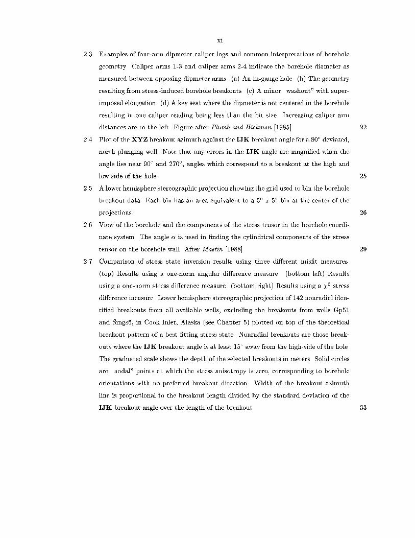
Examples of fourarm dipmeter caliper logs and common interpretations of borehole
geometry Caliper arms and caliper arms indicate the borehole diameter as
measured between opposing dipmeter arms a An ingauge hole b The geometry
resulting from stressinduced borehole breakouts c A minor washout with super
imposed elongation d A key seat where the dipmeter is not centered in the borehole
resulting in one caliper reading being less than the bit size Increasing caliper arm
distances are to the left Figure after Plumb and Hickman
Plot of theXYZ breakout azimuth against the IJK breakout angle for a deviated
north plunging well Note that any errors in the IJK angle are magnied when the
angle lies near and angles which correspond to a breakout at the high and
low side of the hole
A lower hemisphere stereographic projection showing the grid used to bin the borehole
breakout data Each bin has an area equivalent to a x bin at the center of the
projections
View of the borehole and the components of the stress tensor in the borehole coordi
nate system The angle is used in nding the cylindrical components of the stress
tensor on the borehole wall After Mastin
Comparison of stress state inversion results using three di erent mist measures
top Results using a onenorm angular di erence measure bottom left Results
using a onenorm stress di erence measure bottom right Results using a stress
di erence measure Lower hemisphere stereographic projection of nonradial iden
tied breakouts from all available wells excluding the breakouts from wells Gp
and Smgs in Cook Inlet Alaska see Chapter plotted on top of the theoretical
breakout pattern of a best tting stress state Nonradial breakouts are those break
outs where the IJK breakout angle is at least away from the highside of the hole
The graduated scale shows the depth of the selected breakouts in meters Solid circles
are nodal points at which the stress anisotropy is zero corresponding to borehole
orientations with no preferred breakout direction Width of the breakout azimuth
line is proportional to the breakout length divided by the standard deviation of the
IJK breakout angle over the length of the breakout

xii
Histograms of residuals between the borehole breakout data plotted in Figure
and the best tting stress state for a particular mist measure top Histogram
of the residual angular di erence oj mj S in bins using the onenorm angu
lar mist measure inversion results bottom left Histogram of the residual stress
di erence tmaxmj S tmax
oj Sd between the theoretical tmax at the
predicted location of the breakout and tmax at the breakout using the onenorm
stress di erence measure bottom right Histogram of the residual stress di erence
tmaxmj Stmax
oj Sd between the theoretical tmax at the predicted loca
tion of the breakout and tmax at the breakout using the stress di erence measure
Various weighted mist measures plotted as a function of for the borehole breakout
data shown in Figure where the thick solid line is the condence limit for
the inversion the thin solid line is the minimized mist where for each value of the
directions of the principal stress axes are allowed to vary so that the minimum mist
is obtained and the dotted line is the mist using the principal stress directions from
the respective best tting model The condence value is plotted at the constant
solid line top Onenorm angular di erence mists bottom left Onenorm stress
di erence mists bottom right stress di erence mists
Comparison of stress state inversion results using three di erent mist measures
top Results using a onenorm angular di erence measure bottom left Results
using a onenorm stress di erence measure bottom right Results using a stress
di erence measure Lower hemisphere stereographic projection plot where the digits
and show the best tting orientation of the S S and S principal stress axes
for the borehole breakout data plotted in Figure The condence limits of
the S S and S orientations are plotted as thick solid lines thin solid lines and
dotted lines respectively
top Example parameterization of a stress tensor into a binary encoded chromosome
middle Flow diagram of a genetic algorithm bottom Example of the crossover
and mutation operators on chromosomes
Compiled and processed data from the Siljan Deep Drilling Project in Sweden from
Qian and Pedersen plotted on top of the theoretical breakout pattern for their
best tting stress state of SHSv and ShSv where SH lies
east of north Solid circles are nodal points at which the stress anisotropy is zero
corresponding to borehole orientations with no preferred breakout direction The
nodal points for this stress state lie at a deviation of A Poissons ratio of
was used to calculate the breakout pattern The vertical depth scale is in meters

xiii
Histogram of the angular di erence measured in the plane perpendicular to the bore
hole axis between the breakout orientation and the high and low sides of the borehole
for the Qian and Pedersen data
Compiled and processed Qian and Pedersen borehole breakout data plotted
on top of the theoretical breakout pattern for a best tting stress state generated
using the genetic algorithm and Powell optimizer inversion technique Solid circles
are nodal points at which the stress anisotropy is zero corresponding to bore
hole orientations with no preferred breakout direction A Poissons ratio of was
used to calculate the breakout pattern The vertical depth scale is in meters left
Theoretical breakout pattern from the onenorm angular di erence mist measure
inversion right Theoretical breakout pattern from the onenorm stress di erence
mist measure inversion
Results from the reanalysis of the Qian and Pedersen borehole breakout data
Lower hemisphere stereographic projection plot where the digits and show the
optimized orientation of the S S and S principal stress axes respectively The
weighted onenorm mist condence limits of the S S and S orientations
are plotted as thick solid lines thin solid lines and dotted lines respectively left
Inversion using the onenorm angular di erence mist measure The stress state ratio
is held constant at Note that the direction of S is very well constrained but
S and S can lie virtually anywhere within a vertical plane striking NE right
Inversion using the onenorm stress di erence mist measure is held constant at
The best tting principal stress directions are within the condence limits
identied in left gure
Results from the reanalysis of the Qian and Pedersen borehole breakout data
Plot of the weighted onenorm mist as a function of where the thick solid line is
the condence limit the thin solid line is the minimized mist where for each
value of the directions of the principal stress axes are allowed to vary so that the
minimummist is obtained and the dotted line is the mist using the principal stress
directions from the best tting model left Inversion using the onenorm angular
di erence mist measure right Inversion using the onenorm stress di erence mist
measure
Location star of the Point Pedernales eld in the o shore borderland along with some
of the major Quaternary faults in the southern California region LA downtown Los
Angeles SB Santa Barbara SLBF Santa Lucia Bank Fault and HF Hosgri Fault

xiv
Lower hemisphere stereographic projection plots of the azimuth of borehole elongation
at m log depth intervals from the four wells drilled in the Point Pedernales eld
top Lower hemisphere with all the well data plotted bottom Enlargements of the
top gure The graduated depth scale shows the true vertical depth in meters
Plots of the calipercalibrated and declinationcorrected digitized dipmeter data and
derived quantities as a function of log depth from well A top Borehole elongation
direction solid line pad azimuth long dashed line and borehole azimuth short
dashed line middle Borehole deviation bottom Bit size straight solid line
caliper arm solid line and caliper arm dashed line Selected breakout regions
are plotted as horizontal bars showing the depth extent of the breakouts
Histogram of the angular di erence measured in the plane perpendicular to the bore
hole axis between the breakout orientation and the high and low sides of the borehole
for the Point Pedernales data
Compiled and processed Point Pedernales borehole breakout data plotted on top of
the theoretical breakout pattern for a best tting stress state generated using the
genetic algorithm and Powell optimizer inversion technique Solid circles are nodal
points at which the stress anisotropy is zero corresponding to borehole orientations
with no preferred breakout direction A Poissons ratio of was used to calculate
the breakout pattern The vertical depth scale is in meters left Theoretical break
out pattern from the onenorm angular di erence mist measure inversion right
Theoretical breakout pattern from the onenorm stress di erence mist measure in
version
Results from the analysis of the Point Pedernales borehole breakout data Lower
hemisphere stereographic projection plot where the digits and show the opti
mized orientation of the S S and S principal stress axes respectively The
weighted onenorm mist condence limits of the S S and S orientations are plot
ted as thick solid lines thin solid lines and dotted lines respectively left Inversion
using the onenorm angular di erence mist measure The stress state ratio is held
constant at Inner contours are the condence limits right Inversion using
the onenorm stress di erence mist measure is held constant at The
condence limits are smaller than the size of the and digits

xv
Results from the analysis of the Point Pedernales borehole breakout data Plot of
the weighted onenorm mist as a function of where the thick solid line is the
condence limit the thin solid line is the minimized mist where for each value of
the directions of the principal stress axes are allowed to vary so that the minimum
mist is obtained and the dotted line is the mist using the principal stress directions
from the best tting model left Inversion using the onenorm angular di erence
mist measure right Inversion using the onenorm stress di erence mist measure
Lower hemisphere stereographic projection plot of S or SH orientations from studies
performed in the Santa Maria basin and the western Transverse Ranges The contours
are the same and angular di erence condence limits plotted in Figure
The letters AF refer to the stress state results generated by A all the Point Peder
nales breakouts identied in this study B Point Pedernales breakouts identied in
the vertical A well C Feigl et al D Huang E Mount and Suppe
F Varga and Hickman
left Stereographic projection map of Alaska The boxed area in this plot is shown
in the right plot right Mercator projection of Cook Inlet Alaska plotting major
structural faults thick lines minor faults thin lines the oil elds examined in
this study thin ellipses and the o shore oil platforms where deviated boreholes
were drilled from triangles The northern oil eld is Granite Point GP and
the southern oil eld is Middle Ground Shoals MGS From north to south the
platforms are Granite Point Bruce Granite Point Anna Granite Point Granite Point
Middle Ground Shoals Baker and Middle Ground Shoals Dillon
Geologic and terrane map of Cook Inlet Alaska modied from Bunds et al
The Granite Point and Middle Ground Shoals oil elds are shown as small empty
ellipses
Map view of the paths of the wells from the Granite Point G Anna A and Bruce
B platforms Distances are in meters away from top of the Middle Ground Shoals
number redrill borehole
Map view of the paths of the wells from the Baker platform M in the Middle Ground
Shoals eld Distances are in meters away from the top of the Middle Ground Shoals
number redrill borehole
Map view of the paths of the wells from the Dillon D platform in the Middle Ground
Shoals eld Distances are in meters away from the top of the Middle Ground Shoals
number redrill borehole

xvi
Stress inversion results in Cook Inlet Alaska using all identied breakouts from all
available wells excluding the breakouts from wells Gp and Smgs upper left
Statistics of the breakouts in this data set in the results of the inversion upper
right Lower hemisphere stereographic projection of the breakouts plotted on top of
the theoretical breakout pattern of the best tting stress state The graduated scale
shows the depth of the selected breakouts in meters Solid circles are nodal points
at which the stress anisotropy is zero corresponding to borehole orientations with no
preferred breakout direction lower left Lower hemisphere stereographic projection
in which the digits and show the optimized orientation of the S S and
S principal stress axes respectively The weighted onenorm mist condence
limits of the S S and S orientations are plotted as thick solid lines thin solid lines
and dotted lines respectively The stress state ratio was held constant at
lower right The weighted onenorm mist for the breakouts as a function of where
the thick solid line is the condence limit for this inversion the thin solid line is
the minimized mist where for each value of the directions of the principal stress
axes are allowed to vary so that the minimum mist is obtained and the dotted line
is the mist using the principal stress directions from the best tting model
Stress inversion results in Cook Inlet Alaska using all identied breakouts from all
available wells excluding the breakouts from wells Gp and Smgs Plotting conven
tions are the same as Figure
Stress inversion results in Cook Inlet Alaska using all nonradial identied breakouts
from all availablewells excluding the breakouts fromwells Gp and Smgs Nonradial
breakouts are those breakouts where the IJK breakout angle is at least away from
the highside of the hole Plotting conventions are the same as Figure
Stress inversion results in Cook Inlet Alaska using all nonradial identied breakouts
between and m TVD from available wells excluding the breakouts from
Gp and Smgs Nonradial breakouts are those breakouts where the IJK breakout
angle is at least away from the highside of the hole Plotting conventions are the
same as Figure

xvii
Stress inversion results in Cook Inlet Alaska using all nonradial identied breakouts
between and m TVD from available wells excluding the breakouts from
Gp and Smgs Nonradial breakouts are those breakouts where the IJK breakout
angle is at least away from the highside of the hole Plotting conventions are the
same as Figure

xviii
Stress inversion results in Cook Inlet Alaska using all nonradial identied breakouts
between and m TVD from available wells excluding the breakouts from
Gp and Smgs Nonradial breakouts are those breakouts where the IJK breakout
angle is at least away from the highside of the hole Plotting conventions are the
same as Figure
Stress inversion results in Cook Inlet Alaska using all identied breakouts from all
of the wells drilled into the Granite Point oil eld excluding the breakouts from well
Gp Plotting conventions are the same as Figure
Stress inversion results in Cook Inlet Alaska using all identied breakouts from all
of the wells drilled into the Granite Point oil eld excluding the breakouts from well
Gp Plotting conventions are the same as Figure
Stress inversion results in Cook Inlet Alaska using all identied nonradial breakouts
from all of the wells drilled into the Granite Point oil eld excluding the breakouts
from well Gp Nonradial breakouts are those breakouts where the IJK breakout
angle is at least away from the highside of the hole Plotting conventions are the
same as Figure

xix
Stress inversion results in Cook Inlet Alaska using all nonradial identied breakouts
between and m TVD from all of the wells drilled into the Granite Point
oil eld excluding the breakouts from well Gp Nonradial breakouts are those
breakouts where the IJK breakout angle is at least away from the highside of
the hole Plotting conventions are the same as Figure
Stress inversion results in Cook Inlet Alaska using all identied breakouts from wells
drilled from the Baker platform in the Middle Ground Shoals oil eld Plotting
conventions are the same as Figure
Stress inversion results in Cook Inlet Alaska using all identied breakouts from wells
drilled from the Baker platform in the Middle Ground Shoals oil eld Plotting
conventions are the same as Figure
Stress inversion results in Cook Inlet Alaska using all nonradial identied breakouts
from wells drilled from the Baker platform in the Middle Ground Shoals oil eld
Nonradial breakouts are those breakouts where the IJK breakout angle is at least
away from the highside of the hole Plotting conventions are the same as Figure

xx
Stress inversion results in Cook Inlet Alaska using all identied breakouts occurring
in the BSS formation from wells drilled into the Middle Ground Shoals oil eld
from the Baker platform Plotting conventions are the same as Figure
Stress inversion results in Cook Inlet Alaska using all identied breakouts occurring
in the BSS formation from wells drilled into the Middle Ground Shoals oil eld
from the Baker platform Plotting conventions are the same as Figure
Stress inversion results in Cook Inlet Alaska using all nonradial identied breakouts
occurring in the BSS formation from wells drilled into the Middle Ground Shoals
oil eld from the Baker platform Nonradial breakouts are those breakouts where
the IJK breakout angle is at least away from the highside of the hole Plotting
conventions are the same as Figure
Stress inversion results in Cook Inlet Alaska using all nonradial identied breakouts
occurring in the BSS formation from wells drilled into the Middle Ground Shoals
oil eld from the Baker platform Nonradial breakouts are those breakouts where
the IJK breakout angle is at least away from the highside of the hole Plotting
conventions are the same as Figure
Stress inversion results in Cook Inlet Alaska using all identied breakouts occurring
in the D formation from wells drilled into the Middle Ground Shoals oil eld from the
Baker platform Plotting conventions are the same as Figure
Stress inversion results in Cook Inlet Alaska using all identied breakouts occurring
in the D formation from wells drilled into the Middle Ground Shoals oil eld from the
Baker platform Plotting conventions are the same as Figure
Stress inversion results in Cook Inlet Alaska using all nonradial identied breakouts
occurring in the D formation from wells drilled into the Middle Ground Shoals oil
eld from the Baker platform Nonradial breakouts are those breakouts where the
IJK breakout angle is at least away from the highside of the hole Plotting
conventions are the same as Figure

xxi
Stress inversion results in Cook Inlet Alaska using all identied breakouts occurring
in the G and G formations from wells drilled into the Middle Ground Shoals oil
eld from the Baker platform Plotting conventions are the same as Figure
Stress inversion results in Cook Inlet Alaska using all identied breakouts occurring
in the G and G formations from wells drilled into the Middle Ground Shoals oil
eld from the Baker platform Plotting conventions are the same as Figure
Stress inversion results in Cook Inlet Alaska using all nonradial identied breakouts
occurring in the G and G formations from wells drilled into the Middle Ground
Shoals oil eld from the Baker platform Nonradial breakouts are those breakouts
where the IJK breakout angle is at least away from the highside of the hole
Plotting conventions are the same as Figure
Stress inversion results in Cook Inlet Alaska using all nonradial identied breakouts
between and m TVD from wells drilled from the Baker platform in the
Middle Ground Shoals oil eld Nonradial breakouts are those breakouts where the
IJK breakout angle is at least away from the highside of the hole Plotting
conventions are the same as Figure

xxii
Stress inversion results in Cook Inlet Alaska using all nonradial identied breakouts
between and m TVD from wells drilled from the Baker platform in the
Middle Ground Shoals oil eld Nonradial breakouts are those breakouts where the
IJK breakout angle is at least away from the highside of the hole Plotting
conventions are the same as Figure
Stress inversion results in Cook Inlet Alaska using all identied breakouts from wells
drilled from the Dillon platform in the Middle Ground Shoals oil eld excluding the
breakouts from well Smgs Plotting conventions are the same as Figure
Stress inversion results in Cook Inlet Alaska using all identied breakouts from wells
drilled from the Dillon platform in the Middle Ground Shoals oil eld excluding the
breakouts from well Smgs Plotting conventions are the same as Figure

xxiii
Stress inversion results in Cook Inlet Alaska using all nonradial identied breakouts
from wells drilled from the Dillon platform in the Middle Ground Shoals oil eld
excluding the breakouts from well Smgs Nonradial breakouts are those breakouts
where the IJK breakout angle is at least away from the highside of the hole
Plotting conventions are the same as Figure
Stress inversion results in Cook Inlet Alaska using all nonradial identied breakouts
from wells drilled from the Dillon platform in the Middle Ground Shoals oil eld
excluding the breakouts from well Smgs Nonradial breakouts are those breakouts
where the IJK breakout angle is at least away from the highside of the hole
Plotting conventions are the same as Figure
Stress inversion results in Cook Inlet Alaska using all identied breakouts from wells
drilled from the Dillon platform in the Middle Ground Shoals oil eld excluding
the breakouts from wells Smgs and Smgs Plotting conventions are the same as
Figure
Stress inversion results in Cook Inlet Alaska using all identied breakouts from wells
drilled from the Dillon platform in the Middle Ground Shoals oil eld excluding
the breakouts from wells Smgs and Smgs Plotting conventions are the same as
Figure
Stress inversion results in Cook Inlet Alaska using all nonradial identied breakouts
from wells drilled from the Dillon platform in the Middle Ground Shoals oil eld
excluding the breakouts from wells Smgs and Smgs Nonradial breakouts are those
breakouts where the IJK breakout angle is at least away from the highside of
the hole Plotting conventions are the same as Figure
Stress inversion results in Cook Inlet Alaska using all identied breakouts occurring in
the TE formation from wells drilled from the Dillon platform in the Middle Ground
Shoals oil eld excluding the breakouts from well Smgs Plotting conventions are
the same as Figure

xxiv
Stress inversion results in Cook Inlet Alaska using all identied breakouts occurring in
the TE formation from wells drilled from the Dillon platform in the Middle Ground
Shoals oil eld excluding the breakouts from well Smgs Plotting conventions are
the same as Figure
Stress inversion results in Cook Inlet Alaska using all nonradial identied breakouts
between and m TVD from wells drilled from the Dillon platform in the
Middle Ground Shoals oil eld excluding the breakouts from well Smgs Nonradial
breakouts are those breakouts where the IJK breakout angle is at least away from
the highside of the hole Plotting conventions are the same as Figure
Stress inversion results in Cook Inlet Alaska using all nonradial identied breakouts
between and m TVD from wells drilled from the Dillon platform in the
Middle Ground Shoals oil eld excluding the breakouts from well Smgs Nonradial
breakouts are those breakouts where the IJK breakout angle is at least away from
the highside of the hole Plotting conventions are the same as Figure

xxv
Depth variation of the nonradial Granite Point stress mist stress inversion results
left The gure number refers to the gure containing all of the plots and information
regarding this inversion n is the number of breakouts and l is the total length of the
n breakouts in the inversion middle Lower hemisphere stereographic projection
plot where the digits and show the optimized orientation of the S S and
S principal stress axes respectively The weighted onenorm mist condence
limits of the S S and S orientations are plotted as thick solid lines thin solid
lines and dotted lines respectively The stress state ratio was held constant at the
minimum of the mist versus curve on the right right The weighted onenorm
mist for the breakouts as a function of where the thick solid line is the minimized
mist when is held constant and the principal stress directions are unconstrained
and the dotted line is the mist using the principal stress directions from the best
tting model A rotation of around an axis trending NE and plunging
is required to bring the shallower stress state in alignment with the deeper one
Depth variation of the nonradial Baker Platform stress mist stress inversion results
The S and S condence contours in the m TVD depth range are
almost identical and plot on top of each other Plotting conventions are the same as
in Figure
Comparison of nonradial Baker Platform stress mist stress inversion results from
breakouts occurring in di erent markers and between the D and G markers The
true vertical depth range shown for each marker shows the maximum vertical extent
of the breakouts from each marker Breakouts not in the marker but within the depth
range are not included A rotation of around an axis trending NE and
plunging is required to bring the stress state determined by the BSS breakouts
into alignment with the stress state from the breakouts identied in the D marker
Plotting conventions are the same as in Figure
Comparison of the nonradial Dillon Platform stress mist stress inversion results
Plotting conventions are the same as in Figure
Comparison of the nonradial Cook Inlet stress mist stress inversion results in m
increments from to m TVD Plotting conventions are the same as in Fig
ure

xxvi
Comparison of chosen best tting stress mist stress states from each platform or
oil eld No stress state inversion included breakouts from Gp and Smgs top
Granite Point using radial and nonradial borehole breakouts second from top Baker
platform using the nonradial and radial borehole breakouts third from top Dil
lon platform using the nonradial and radial borehole breakouts excluding the Smgs
breakout bottom Stress state results using nonradial borehole breakouts from all
Cook Inlet wells Plotting conventions are the same as in Figure
Mercator projection plot of the maximum principal stress direction projected to the
horizontal across Alaska obtained from di erent stress measurements including bore
hole breakouts volcanic indicators and earthquake focal mechanisms Stress orienta
tions are from this thesis Estabrook and Jacob and Jolly et al Vectors
are velocities of the Pacic Plate relative to North America in centimeters per year
DeMets et al Quality of data ranking system from Zoback and Zoback
The boxed area is the area shown in Figure
Mercator projection plot of the maximum principal stress direction projected to the
horizontal around Cook Inlet Alaska obtained from di erent stress measurements
including borehole breakouts volcanic indicators and earthquake focal mechanisms
Stress orientations are from this thesis Estabrook and Jacob and Jolly et al
This gure does not include earthquake focal mechanism stress state inversions
where the focal mechanisms cover a large geographic area Vector is velocity of the
Pacic Plate relative to North America in centimeters per year DeMets et al
Quality of data ranking system from Zoback and Zoback
B Plots of the calipercalibrated and declinationcorrected digitized dipmeter and de
rived quantities data as a function of well depth from well Gprd top Borehole
elongation direction solid line pad azimuth dotted line and borehole azimuth
dashed line middle Borehole deviation solid curve and location of marker hori
zons vertical lines with labels bottom Bit size straight solid line caliper arm
solid line and caliper arm dotted line Selected breakout regions are plotted as
horizontal bars showing the depth extent of the breakouts
B Lower hemisphere stereographic projection plots of the selected breakouts from well
Gprd Line widths are proportional to the breakout length left All selected
breakouts right All nonradial breakouts where the IJK breakout angle is not within
of the high side of the hole

xxvii
B Lower hemisphere stereographic projection plots of the selected breakouts from well
Gprd in marker TXSS Line widths are proportional to the breakout length
left All selected breakouts in TXSS right All nonradial breakouts in TXSS
where the IJK breakout angle is not within of the high side of the hole
B Plots of the calipercalibrated and declinationcorrected digitized dipmeter and de
rived quantities data as a function of well depth from well Gprd top Borehole
elongation direction solid line pad azimuth dotted line and borehole azimuth
dashed line middle Borehole deviation solid curve and location of marker hori
zons vertical lines with labels bottom Bit size straight solid line caliper arm
solid line and caliper arm dotted line Selected breakout regions are plotted as
horizontal bars showing the depth extent of the breakouts
B Lower hemisphere stereographic projection plots of the selected breakouts from well
Gprd Line widths are proportional to the breakout length left All selected
breakouts right All nonradial breakouts where the IJK breakout angle is not
within of the high side of the hole
B Lower hemisphere stereographic projection plots of all nonradial breakouts from well
Gprd between the true vertical depths of m on the left and m
on the right
B Plots of the calipercalibrated and declinationcorrected digitized dipmeter and de
rived quantities data as a function of well depth from well Gprd top Borehole
elongation direction solid line pad azimuth dotted line and borehole azimuth
dashed line middle Borehole deviation solid curve and location of marker hori
zons vertical lines with labels bottom Bit size straight solid line caliper arm
solid line and caliper arm dotted line Selected breakout regions are plotted as
horizontal bars showing the depth extent of the breakouts
B Lower hemisphere stereographic projection plots of the selected breakouts from well
Gprd Line widths are proportional to the breakout length left All selected
breakouts right All nonradial breakouts where the IJK breakout angle is not
within of the high side of the hole
B Plots of the calipercalibrated and declinationcorrected digitized dipmeter and de
rived quantities data as a function of well depth fromwell Gprd le top Borehole
elongation direction solid line pad azimuth dotted line and borehole azimuth
dashed line middle Borehole deviation solid curve and location of marker hori
zons vertical lines with labels bottom Bit size straight solid line caliper arm
solid line and caliper arm dotted line Selected breakout regions are plotted as
horizontal bars showing the depth extent of the breakouts

xxviii
B Plots of the calipercalibrated and declinationcorrected digitized dipmeter and de
rived quantities data as a function of well depth fromwell Gprd le top Borehole
elongation direction solid line pad azimuth dotted line and borehole azimuth
dashed line middle Borehole deviation solid curve and location of marker hori
zons vertical lines with labels bottom Bit size straight solid line caliper arm
solid line and caliper arm dotted line Selected breakout regions are plotted as
horizontal bars showing the depth extent of the breakouts
B Lower hemisphere stereographic projection plots of the selected breakouts from well
Gprd Line widths are proportional to the breakout length left All selected
breakouts right All nonradial breakouts where the IJK breakout angle is not
within of the high side of the hole
B Plots of the calipercalibrated and declinationcorrected digitized dipmeter and de
rived quantities data as a function of well depth from well Gp le top Borehole
elongation direction solid line pad azimuth dotted line and borehole azimuth
dashed line middle Borehole deviation solid curve and location of marker hori
zons vertical lines with labels bottom Bit size straight solid line caliper arm
solid line and caliper arm dotted line Selected breakout regions are plotted as
horizontal bars showing the depth extent of the breakouts
B Lower hemisphere stereographic projection plots of the selected breakouts from well
Gp Line widths are proportional to the breakout length left All selected break
outs right All nonradial breakouts where the IJK breakout angle is not within
of the high side of the hole
B Plots of the calipercalibrated and declinationcorrected digitized dipmeter and de
rived quantities data as a function of well depth from well Gp top Borehole
elongation direction solid line pad azimuth dotted line and borehole azimuth
dashed line middle Borehole deviation solid curve and location of marker hori
zons vertical lines with labels bottom Bit size straight solid line caliper arm
solid line and caliper arm dotted line Selected breakout regions are plotted as
horizontal bars showing the depth extent of the breakouts

xxix
B Lower hemisphere stereographic projection plots of the selected breakouts from well
Gp Line widths are proportional to the breakout length left All selected break
outs right All nonradial breakouts where the IJK breakout angle is not within
of the high side of the hole
B Plots of the calipercalibrated and declinationcorrected digitized dipmeter and de
rived quantities data as a function of well depth from well Gp top Borehole
elongation direction solid line pad azimuth dotted line and borehole azimuth
dashed line middle Borehole deviation solid curve and location of marker hori
zons vertical lines with labels bottom Bit size straight solid line caliper arm
solid line and caliper arm dotted line Selected breakout regions are plotted as
horizontal bars showing the depth extent of the breakouts
B Lower hemisphere stereographic projection plots of the selected breakouts from well
Gp Line widths are proportional to the breakout length left All selected break
outs right All nonradial breakouts where the IJK breakout angle is not within
of the high side of the hole
B Lower hemisphere stereographic projection plots of all nonradial breakouts from well
Gp between the true vertical depths of m
B Plots of the calipercalibrated and declinationcorrected digitized dipmeter and de
rived quantities data as a function of well depth from well Gp top Borehole
elongation direction solid line pad azimuth dotted line and borehole azimuth
dashed line middle Borehole deviation solid curve and location of marker hori
zons vertical lines with labels bottom Bit size straight solid line caliper arm
solid line and caliper arm dotted line Selected breakout regions are plotted as
horizontal bars showing the depth extent of the breakouts
B Lower hemisphere stereographic projection plots of the selected breakouts from well
Gp Line widths are proportional to the breakout length left All selected break
outs right All nonradial breakouts where the IJK breakout angle is not within
of the high side of the hole
B Lower hemisphere stereographic projection plots of all nonradial breakouts from well
Gp between the true vertical depths of m on the left and m
on the right
xxx
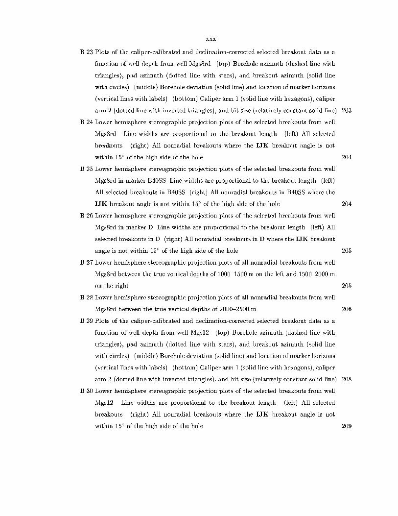
B Plots of the calipercalibrated and declinationcorrected selected breakout data as a
function of well depth from well Mgsrd top Borehole azimuth dashed line with
triangles pad azimuth dotted line with stars and breakout azimuth solid line
with circles middle Borehole deviation solid line and location of marker horizons
vertical lines with labels bottom Caliper arm solid line with hexagons caliper
arm dotted line with inverted triangles and bit size relatively constant solid line
B Lower hemisphere stereographic projection plots of the selected breakouts from well
Mgsrd Line widths are proportional to the breakout length left All selected
breakouts right All nonradial breakouts where the IJK breakout angle is not
within of the high side of the hole
B Lower hemisphere stereographic projection plots of the selected breakouts from well
Mgsrd in marker BSS Line widths are proportional to the breakout length left
All selected breakouts in BSS right All nonradial breakouts in BSS where the
IJK breakout angle is not within of the high side of the hole
B Lower hemisphere stereographic projection plots of the selected breakouts from well
Mgsrd in marker D Line widths are proportional to the breakout length left All
selected breakouts in D right All nonradial breakouts in D where the IJK breakout
angle is not within of the high side of the hole
B Lower hemisphere stereographic projection plots of all nonradial breakouts from well
Mgsrd between the true vertical depths of m on the left and m
on the right
B Lower hemisphere stereographic projection plots of all nonradial breakouts from well
Mgsrd between the true vertical depths of m
B Plots of the calipercalibrated and declinationcorrected selected breakout data as a
function of well depth from well Mgs top Borehole azimuth dashed line with
triangles pad azimuth dotted line with stars and breakout azimuth solid line
with circles middle Borehole deviation solid line and location of marker horizons
vertical lines with labels bottom Caliper arm solid line with hexagons caliper
arm dotted line with inverted triangles and bit size relatively constant solid line
B Lower hemisphere stereographic projection plots of the selected breakouts from well
Mgs Line widths are proportional to the breakout length left All selected
breakouts right All nonradial breakouts where the IJK breakout angle is not
within of the high side of the hole

xxxi
B Lower hemisphere stereographic projection plots of the selected breakouts from well
Mgs in marker D Line widths are proportional to the breakout length left All
selected breakouts in D right All nonradial breakouts in D where the IJK breakout
angle is not within of the high side of the hole
B Lower hemisphere stereographic projection plots of the selected breakouts from well
Mgs in markers G and G Line widths are proportional to the breakout length
left All selected breakouts in G and G right All nonradial breakouts in G and
G where the IJK breakout angle is not within of the high side of the hole
B Lower hemisphere stereographic projection plots of all nonradial breakouts from well
Mgs between the true vertical depths of m on the left and m
on the right
B Plots of the calipercalibrated and declinationcorrected selected breakout data as a
function of well depth from well Mgs top Borehole azimuth dashed line with
triangles pad azimuth dotted line with stars and breakout azimuth solid line
with circles middle Borehole deviation solid line and location of marker horizons
vertical lines with labels bottom Caliper arm solid line with hexagons caliper
arm dotted line with inverted triangles and bit size relatively constant solid line
B Lower hemisphere stereographic projection plots of the selected breakouts from well
Mgs Line widths are proportional to the breakout length left All selected
breakouts right All nonradial breakouts where the IJK breakout angle is not
within of the high side of the hole
B Lower hemisphere stereographic projection plots of the selected breakouts from well
Mgs in marker BSS Line widths are proportional to the breakout length left
All selected breakouts in BSS right All nonradial breakouts in BSS where the
IJK breakout angle is not within of the high side of the hole
B Lower hemisphere stereographic projection plots of the selected breakouts from well
Mgs in markers G and G Line widths are proportional to the breakout length
left All selected breakouts in G and G right All nonradial breakouts in G and
G where the IJK breakout angle is not within of the high side of the hole
B Lower hemisphere stereographic projection plots of all nonradial breakouts from well
Mgs between the true vertical depths of m on the left and m
on the right
B Lower hemisphere stereographic projection plots of all nonradial breakouts from well
Mgs between the true vertical depths of m

xxxii
B Plots of the calipercalibrated and declinationcorrected selected breakout data as a
function of well depth from well Mgs top Borehole azimuth dashed line with
triangles pad azimuth dotted line with stars and breakout azimuth solid line
with circles middle Borehole deviation solid line and location of marker horizons
vertical lines with labels bottom Caliper arm solid line with hexagons caliper
arm dotted line with inverted triangles and bit size relatively constant solid line
B Lower hemisphere stereographic projection plots of the selected breakouts from well
Mgs Line widths are proportional to the breakout length left All selected
breakouts right All nonradial breakouts where the IJK breakout angle is not
within of the high side of the hole
B Lower hemisphere stereographic projection plots of the selected breakouts from well
Mgs in markers G and G Line widths are proportional to the breakout length
left All selected breakouts in G and G right All nonradial breakouts in G and
G where the IJK breakout angle is not within of the high side of the hole
B Lower hemisphere stereographic projection plots of all nonradial breakouts from well
Mgs between the true vertical depths of m on the left and m
on the right
B Plots of the calipercalibrated and declinationcorrected selected breakout data as a
function of well depth from well Mgs top Borehole azimuth dashed line with
triangles pad azimuth dotted line with stars and breakout azimuth solid line
with circles middle Borehole deviation solid line and location of marker horizons
vertical lines with labels bottom Caliper arm solid line with hexagons caliper
arm dotted line with inverted triangles and bit size relatively constant solid line
B Lower hemisphere stereographic projection plots of the selected breakouts from well
Mgs Line widths are proportional to the breakout length left All selected
breakouts right All nonradial breakouts where the IJK breakout angle is not
within of the high side of the hole
B Lower hemisphere stereographic projection plots of the selected breakouts from well
Mgs in marker BSS Line widths are proportional to the breakout length left
All selected breakouts in BSS right All nonradial breakouts in BSS where the
IJK breakout angle is not within of the high side of the hole
B Lower hemisphere stereographic projection plots of the selected breakouts from well
Mgs in marker D Line widths are proportional to the breakout length left All
selected breakouts in D right All nonradial breakouts in D where the IJK breakout
angle is not within of the high side of the hole

xxxiii
B Lower hemisphere stereographic projection plots of the selected breakouts from well
Mgs in markers G and G Line widths are proportional to the breakout length
left All selected breakouts in G and G right All nonradial breakouts in G and
G where the IJK breakout angle is not within of the high side of the hole
B Lower hemisphere stereographic projection plots of all nonradial breakouts from well
Mgs between the true vertical depths of m on the left and m
on the right
B Plots of the calipercalibrated and declinationcorrected selected breakout data as a
function of well depth from well Mgs top Borehole azimuth dashed line with
triangles pad azimuth dotted line with stars and breakout azimuth solid line
with circles middle Borehole deviation solid line and location of marker horizons
vertical lines with labels bottom Caliper arm solid line with hexagons caliper
arm dotted line with inverted triangles and bit size relatively constant solid line
B Lower hemisphere stereographic projection plots of the selected breakouts from well
Mgs Line widths are proportional to the breakout length left All selected
breakouts right All nonradial breakouts where the IJK breakout angle is not
within of the high side of the hole
B Lower hemisphere stereographic projection plots of the selected breakouts from well
Mgs in marker BSS Line widths are proportional to the breakout length left
All selected breakouts in BSS right All nonradial breakouts in BSS where the
IJK breakout angle is not within of the high side of the hole
B Lower hemisphere stereographic projection plots of the selected breakouts from well
Mgs in marker D Line widths are proportional to the breakout length left All
selected breakouts in D right All nonradial breakouts in D where the IJK breakout
angle is not within of the high side of the hole
B Lower hemisphere stereographic projection plots of the selected breakouts from well
Mgs in markers G and G Line widths are proportional to the breakout length
left All selected breakouts in G and G right All nonradial breakouts in G and
G where the IJK breakout angle is not within of the high side of the hole
B Lower hemisphere stereographic projection plots of all nonradial breakouts from well
Mgs between the true vertical depths of m on the left and m
on the right
B Lower hemisphere stereographic projection plots of all nonradial breakouts from well
Mgs between the true vertical depths of m on the left and m
on the right

xxxiv
B Plots of the calipercalibrated and declinationcorrected digitized dipmeter and de
rived quantities data as a function of well depth from well Mgs top Borehole
elongation direction solid line pad azimuth dotted line and borehole azimuth
dashed line middle Borehole deviation solid curve and location of marker hori
zons vertical lines with labels bottom Bit size straight solid line caliper arm
solid line and caliper arm dotted line Selected breakout regions are plotted as
horizontal bars showing the depth extent of the breakouts
B Lower hemisphere stereographic projection plots of the selected breakouts from well
Mgs Line widths are proportional to the breakout length left All selected
breakouts right All nonradial breakouts where the IJK breakout angle is not
within of the high side of the hole
B Lower hemisphere stereographic projection plots of the selected breakouts from well
Mgs in marker D Line widths are proportional to the breakout length left All
selected breakouts in D right All nonradial breakouts in D where the IJK breakout
angle is not within of the high side of the hole
B Lower hemisphere stereographic projection plots of all nonradial breakouts from well
Mgs between the true vertical depths of m on the left and m
on the right
B Lower hemisphere stereographic projection plots of all nonradial breakouts from well
Mgs between the true vertical depths of m
B Plots of the calipercalibrated and declinationcorrected digitized dipmeter and de
rived quantities data as a function of well depth from well Mgs top Borehole
elongation direction solid line pad azimuth dotted line and borehole azimuth
dashed line middle Borehole deviation solid curve and location of marker hori
zons vertical lines with labels bottom Bit size straight solid line caliper arm
solid line and caliper arm dotted line Selected breakout regions are plotted as
horizontal bars showing the depth extent of the breakouts

xxxv
B Lower hemisphere stereographic projection plots of the selected breakouts from well
Mgs Line widths are proportional to the breakout length left All selected
breakouts right All nonradial breakouts where the IJK breakout angle is not
within of the high side of the hole
B Lower hemisphere stereographic projection plots of all nonradial breakouts from well
Mgs between the true vertical depths of m on the left and m
on the right
B Plots of the calipercalibrated and declinationcorrected digitized dipmeter and de
rived quantities data as a function of well depth from well Smgs top Borehole
elongation direction solid line pad azimuth dotted line and borehole azimuth
dashed line middle Borehole deviation solid curve and location of marker hori
zons vertical lines with labels bottom Bit size straight solid line caliper arm
solid line and caliper arm dotted line Selected breakout regions are plotted as
horizontal bars showing the depth extent of the breakouts
B Lower hemisphere stereographic projection plots of the selected breakouts from well
Smgs Line widths are proportional to the breakout length left All selected
breakouts right All nonradial breakouts where the IJK breakout angle is not
within of the high side of the hole
B Lower hemisphere stereographic projection plots of the selected breakouts from well
Smgs in marker TE Line widths are proportional to the breakout length left
All selected breakouts in TE right All nonradial breakouts in TE where the IJK
breakout angle is not within of the high side of the hole
B Lower hemisphere stereographic projection plots of all nonradial breakouts from well
Smgs between the true vertical depths of m on the left and m
on the right
B Lower hemisphere stereographic projection plots of all nonradial breakouts from well
Smgs between the true vertical depths of m on the left and m
on the right
B Lower hemisphere stereographic projection plots of all nonradial breakouts from well
Smgs between the true vertical depths of m

xxxvi
B Plots of the calipercalibrated and declinationcorrected digitized dipmeter and de
rived quantities data as a function of well depth from well Smgs top Borehole
elongation direction solid line pad azimuth dotted line and borehole azimuth
dashed line middle Borehole deviation solid curve and location of marker hori
zons vertical lines with labels bottom Bit size straight solid line caliper arm
solid line and caliper arm dotted line Selected breakout regions are plotted as
horizontal bars showing the depth extent of the breakouts
B Lower hemisphere stereographic projection plots of the selected breakouts from well
Smgs Line widths are proportional to the breakout length left All selected
breakouts right All nonradial breakouts where the IJK breakout angle is not
within of the high side of the hole
B Lower hemisphere stereographic projection plots of all nonradial breakouts from well
Smgs between the true vertical depths of m on the left and m
on the right
B Lower hemisphere stereographic projection plots of all nonradial breakouts from well
Smgs between the true vertical depths of m on the left and m
on the right
B Lower hemisphere stereographic projection plots of all nonradial breakouts from well
Smgs between the true vertical depths of m
B Lower hemisphere stereographic projection plots of the selected breakouts from well
Smgs Line widths are proportional to the breakout length left All selected
breakouts right All nonradial breakouts where the IJK breakout angle is not
within of the high side of the hole
B Plots of the calipercalibrated and declinationcorrected digitized dipmeter and de
rived quantities data as a function of well depth from well Smgs top Borehole
elongation direction solid line pad azimuth dotted line and borehole azimuth
dashed line middle Borehole deviation solid curve and location of marker hori
zons vertical lines with labels bottom Bit size straight solid line caliper arm
solid line and caliper arm dotted line Selected breakout regions are plotted as
horizontal bars showing the depth extent of the breakouts

xxxvii
B Plots of the calipercalibrated and declinationcorrected digitized dipmeter and de
rived quantities data as a function of well depth from well Smgs top Borehole
elongation direction solid line pad azimuth dotted line and borehole azimuth
dashed line middle Borehole deviation solid curve and location of marker hori
zons vertical lines with labels bottom Bit size straight solid line caliper arm
solid line and caliper arm dotted line Selected breakout regions are plotted as
horizontal bars showing the depth extent of the breakouts
B Lower hemisphere stereographic projection plots of the selected breakouts from well
Smgs Line widths are proportional to the breakout length left All selected
breakouts right All nonradial breakouts where the IJK breakout angle is not
within of the high side of the hole
B Lower hemisphere stereographic projection plots of the selected breakouts from well
Smgs in marker TE Line widths are proportional to the breakout length left
All selected breakouts in TE right All nonradial breakouts in TE where the IJK
breakout angle is not within of the high side of the hole

xxxviii
List of Tables
Comparison of stress state inversion results using three di erent mist measures
Characteristics of the stress state that minimized the weighted onenorm angular
di erence mist of the Qian and Pedersen borehole breakout data
Characteristics of the stress state that minimized the weighted onenorm stress dif
ference mist of the Qian and Pedersen borehole breakout data
Digitized well logs from the Unocal Company of wells drilled o shore from Point
Pedernales California in the Santa Maria Basin
Characteristics of the stress state that minimized the weighted onenorm angular
di erence mist of the Point Pedernales borehole breakout data
Characteristics of the stress state that minimized the weighted onenorm stress dif
ference mist of the Point Pedernales borehole breakout data
Stress state results from studies performed in the Santa Maria basin and the western
Transverse Ranges
Well log data that were analyzed for breakouts
Statistics of various selected subsets of breakouts
Stress state results from studies performed in southcentral Alaska
B List of the breakouts identied in two separate dipmeter runs over the to m
log foot depth interval in Gprd with le on the left and le on the right The
identied IJK breakout angle results from the two log les agree within
B List of the breakouts identied in two separate dipmeter runs over the to m
log foot depth interval in Gp with le on the left and le on the right The
identied IJK breakout angle results from the two log les agree within

Chapter Introduction
Objective and Motivation
An understanding of the state of stress in the earth is important for many di erent elds including
plate tectonics oil production seismic hazards and mining Improvements in the knowledge of
regional states of stress provide baseline stress measurements for understanding future earthquakes
and comparing the state of stress before and after earthquakes The stress state is also important in
understanding seismic and aseismic faulting and the rheology of crustal and upper mantle materials
Assessments of seismic hazards mine stability and underground waste containment Stock et al
all require stress measurements Finally the state of stress plays an important role in many
di erent aspects of oil production including proper well path design to most e ectively produce oil
and avoid borehole failure Addis et al Peska and Zoback using proper mud weight to
avoid borehole failure Addis et al and the prediction of the direction of hydraulic fractures
Currently many di erent data are available for determining the stress in the earth including fault
slip data Angelier Michael focal mechanisms Michael stress induced borehole
breakouts Zajac and Stock this thesis and insitu hydraulic fractures eg Haimson
and Fairhurst Stock et al This thesis introduces a new method of constraining the
vector directions of the three principal stresses and their relative magnitudes by using borehole
breakouts identied in many di erently oriented nonvertical boreholes Borehole breakouts are
two zones on opposites sides of an otherwise cylindrical borehole where fracture and spalling have
enlarged it in cross section from a circular to roughly an elliptical shape Figure Mastin
I begin by reviewing some of the previous work in understanding borehole breakout formation and
in utilizing borehole breakouts to constrain the regional stress state The rst studies of the shape of
the borehole wall using fourarm dipmeters showed that borehole breakouts are a common feature
in boreholes and showed a consistent orientation over large geographic areas Bell and Gough
Bell and Gough examined a highly consistent data set of NWSE oriented borehole breakout
observations from Alberta western Canada observed over a x km region Bell and Gough
assumed that one of the principal stress directions was vertical and that the breakouts will form
centered at the azimuth of greatest compressive stress at the borehole wall The Kirsch equations
that describe the stress concentration around a circular hole in a stressed medium show that the
location of the greatest compressive stress on the borehole wall occurs away from the orientation
of the fareld horizontal maximum principal stress direction The orientation of borehole breakouts

Breakout
Breakout
Hydrofrac Hydrofrac
Sh
SH
Sh
SH
Figure Cross section of a borehole showing the predicted orientation of the minimum andmaximum principal stress directions and the locations of borehole breakouts and hydrofractures inthe borehole assuming that the borehole axis is parallel to one of the principal stress directionsBorehole breakout shapes are highly irregular and may not appear as the breakouts shown in thisgure
thus constrains the directions of the minimum horizontal principal stress Sh and the maximum
horizontal stress SH Bell and Gough concluded that the NWSE oriented breakouts are due
to a NESW directed maximum horizontal principal stress which is normal to the Rocky Mountain
fold axes suggesting that the stress state responsible for the thrust faulting in the mountains is still
present Following Bell and Goughs work highly localized studies using breakouts such as
the stress prole as a function of depth near the San Andreas fault zone Shamir and Zoback
and regional to global studies Zoback et al have been performed Stress orientation results
from borehole breakouts have been shown to be consistent with other indicators of stress direction
such as hydraulic fractures earthquake focal mechanisms and overcoring measurements on both
local and regional scales eg Bell and Gough Zoback and Zoback Gough and
Bell Plumb and Hickman Stock et al Zoback et al Zoback and Healy
Zoback
In addition to the stress state studies using borehole breakouts the last two decades have seen
much research into the formation of borehole breakouts Gough and Bell applied brittle
shear fracture theory to the borehole wall and predicted pairs of conjugate shear fractures that
are tangential to the borehole wall and oriented to the maximum horizontal principal
stress direction where is the angle of internal friction of the rock The shear fractures intersect
and create sharp pointed dog eared breakouts Since Gough and Bell s study borehole
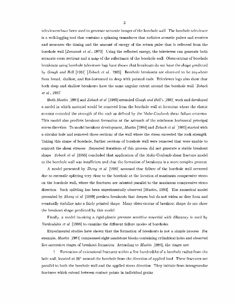
televiewers have been used to generate accurate images of the borehole wall The borehole televiewer
is a welllogging tool that contains a spinning transducer that radiates acoustic pulses and receives
and measures the timing and the amount of energy of the return pulse that is reected from the
borehole wall Zemanek et al Using the reected energy the televiewer can generate both
accurate cross sections and a map of the reectance of the borehole wall Observations of borehole
breakouts using borehole televiewer logs have shown that breakouts do not have the shape predicted
by Gough and Bell Zoback et al Borehole breakouts are observed to be anywhere
from broad shallow and atbottomed to deep with pointed ends Televiewer logs also show that
both deep and shallow breakouts have the same angular extent around the borehole wall Zoback
et al
BothMastin and Zoback et al extended Gough and Bell s work and developed
a model in which material would be removed from the borehole wall at locations where the elastic
stresses exceeded the strength of the rock as dened by the MohrCoulomb shear failure criterion
This model also predicts breakout formation at the azimuth of the minimum horizontal principal
stress direction To model breakout developmentMastin and Zoback et al started with
a circular hole and removed those sections of the wall where the stress exceeded the rock strength
Taking this shape of borehole further sections of borehole wall were removed that were unable to
support the shear stresses Repeated iterations of this process did not generate a stable breakout
shape Zoback et al concluded that application of the MohrCoulomb shear fracture model
to the borehole wall was insucient and that the formation of breakouts is a more complex process
A model presented by Zheng et al assumed that failure of the borehole wall occurred
due to extensile splitting very close to the borehole at the location of maximum compressive stress
on the borehole wall where the fractures are oriented parallel to the maximum compressive stress
direction Such splitting has been experimentally observed Mastin The numerical model
presented by Zheng et al predicts breakouts that deepen but do not widen as they form and
eventually stabilize into a fairly pointed shape Many observations of breakout shape do not show
the breakout shape predicted by this model
Finally a model invoking a rigidplastic pressure sensitive material with dilatancy is used by
Vardoulakis et al to examine the di erent failure modes of boreholes
Experimental studies have shown that the formation of breakouts is not a simple process For
exampleMastin compressed eight sandstone blocks containing cylindrical holes and observed
ve successive stages of breakout formation According to Mastin the stages are
Formation of extensional fractures within a few hundredths of a borehole radius from the
hole wall located at around the borehole from the direction of applied load These fractures are
parallel to both the borehole wall and the applied stress direction They initiate from intragranular
fractures which extend between contact points in individual grains

Buckling of the thin rock slab between the fracture and the wellbore This causes the
fractures to propagate toward and intersect the borehole wall forming small thrusted wedges that
are sheared into the wellbore The breaking o of these wedges exposes a spalled area bounded by
the location of the former extensional fracture andor by a small scarp on one side of the spalled
area where the wedge broke o
Disaggregation of rock inside the breakout andor formation of more extensional frac
tures parallel to the initial one father away from the wellbore Extensional fractures link together
at their ends to form two shear surfaces that converge in the direction away from the borehole wall
Expulsion of the material between these surfaces by shearing into the borehole The
resulting breakout is vshaped to cuspate in cross section and approximately as wide as the initial
spalled area in step
Development of a zone of inelastic yielding around the breakout composed of fractured
and disaggregated grain particles The archlike shape of the breakout tip prevents expulsion of this
material thereby inhibiting further growth In some cases fractures extend from the side of this
zone toward the borehole wall
Regardless of the exact model of breakout formation it is generally held that the location of
the breakouts on the borehole wall corresponds to the location of the maximum compressive stress
concentration Commonly breakout data are used to constrain directions of stress but not their
relative magnitudes If hydrofracture and the mechanical properties of core samples are available
the magnitudes of the principal stresses can be estimated Vernik and Zoback Peska and
Zoback However in principle the presence of breakouts can also yield information on stress
magnitudes both because the presence of a breakout indicates that the hoop stress exceeds the
yield strength of the rock and because when the borehole is not aligned with a principal stress axis
the breakout orientation depends on the relative magnitudes of all three principal stresses as well
as on the orientations of the stresses Thus additional information about the stress tensor can be
obtained from the directions of breakouts in deviated nonvertical drill holes one can estimate the
directions of all three principal stresses and provide some constraint on their relative magnitudes
Such a technique provides a more complete knowledge of the stress tensor and works even if none
of the principal stresses is vertical
The smallest data set applicable to this technique would most likely consist of a few closely
spaced variably oriented wells logged with oriented caliper arm data O shore oil platforms provide
good sources of such data since the wells are drilled in many directions and at nonvertical deviations
to fully develop the oil elds Depending upon the number of wells and the horizontal extent of
the caliper data this technique determines a regional stress state localized over a spatial extent of
kilometers to tens of kilometers
Other authors have presented di erent techniques using deviated boreholes to determine the local

stress state Qian and Pedersen applied a nonlinear inversion technique to a set of borehole
breakout data Aadnoy a b examined fractures in deviated boreholes Peska and Zoback
developed a technique using leako tests microfracturemeasurements pore pressure measurements
breakout and tensile fractures with theoretical borehole failure calculations to determine the stress
directions and magnitudes from a single deviated well Neither the technique of Peska and Zoback
nor the technique presented in this paper assumes a vertical principal stress direction Multiple
applications of the Peska and Zoback technique over a region would yield a more regional
stress tensor
The theoretical basis of this technique has been recognized for nearly a decade but it has only
been applied in a few areas perhaps because of the lack of strongly deviated drill holes in most
regions It is based on the elastic equations for stress surrounding an arbitrarily oriented cylindrical
hole in a medium with known fareld stresses Equations for the stress eld surrounding a circular
hole in an elastic plate subjected to plane strain are given by Kirsch and various other
authors eg Hubbert and Willis Timoshenko and Goodier Jaeger and Cook
The equations for the stress components at the wall of a cylindrical hole in a polyaxial stress eld
are given by Hiramatsu and Oka Youngdahl and Sternberg Fairhurst Daneshy
Richardson Mastin and Qian and Pedersen
If a drill hole is parallel to one of the principal stress directions the rock strength and the relative
magnitudes of the remaining two stresses a ect the presence or absence of breakouts but not their
azimuth in the borehole reference frame The magnitudes of the principal stresses must be inferred
by another technique rather than just by observations of breakout orientation
The nal azimuthal extent or width of the breakout after breakout formation is thought by
some authors to be controlled by the relative magnitudes of the principal stresses so that if one
of the principal horizontal stresses is known and the rock strength is known or estimated the
magnitude of the other principal horizontal stress can be estimated Moos and Zoback Vernik
and Zoback However other authors have argued that this may not be the case because the
angle subtended by the breakout may vary with the stress history Zheng et al The angle
subtended by a breakout may also depend on the mode of failure during breakout formation which
is still debated as mentioned above
However in a nonvertical hole or a hole oriented obliquely to the three principal stress directions
one does not necessarily need independent measurements of one principal stress to infer the relative
magnitudes of another principal stress because the magnitudes of the principal stresses as well
as their directions inuence the position of the maximum compressive stress at the borehole wall
Richardson and hence the position at which breakouts would form This fact was further
elaborated by Mastin who showed stereographic projections Hobbs et al indicating
the direction of breakouts expected in variably oriented drill holes for di erent stress orientations

North
Up
East
Breakout
Boreholedeviation
S
EW
N
Breakout
Borehole azimuth(trend)
Ω
Ωδ
δ
Breakout azimuth(trend)
Figure Relationship between an arbitrarily oriented borehole containing a breakout and howthis borehole and its breakout orientation would be plotted on a lower hemisphere stereograph ofborehole azimuth and deviation The breakouts on either side of the borehole are assumed to be onopposite sides of the borehole and hence there exists a single plane which contains the borehole axisand the locus of breakouts The intersection of this plane with the horizontal plane denes a linewhich plots as the orientation of the breakout in the lower hemisphere stereographic projection plot
and principal stress magnitudes Thus if several drill holes of di erent deviations are present in
a given area and if these drill holes are subject to the same stress tensor the orientations of the
breakouts in these holes may provide strong constraints on the orientations and magnitudes of the
principal stresses at that location Zajac and Stock
To plot the breakout data from arbitrarily oriented boreholes and the calculated breakout posi
tions for theoretical fareld stress states lower hemisphere stereographic projections of the borehole
azimuth and deviation eg Figures and are used
This dependence of breakout position on the fareld tectonic stress is illustrated in Figure
where I show patterns of breakout orientations that would be predicted for arbitrarily oriented drill
holes subjected to characteristic stress elds These are similar to the quadrant plots of Mastin
and illustrate the degree to which an inversion or forward modeling of borehole breakout
observations would constrain the stress regime for a given distribution of borehole orientations The
characteristic stress elds are dened by the orientations of the principal stresses S S and S and
the stress ratio
S SS S
where S is the maximum compressive stress S is the intermediate stress and S is the minimum
compressive stress
Note that given enough variation in borehole orientations the stress state can be reasonably
constrained since the patterns vary continuously from an entirely radial distribution of breakout
azimuths for degenerate thrust faulting SH Sh Sv to an entirely circumferential distribution

Top of Borehole
Map view of Borehole0 1 km
Figure Map view of a hypothetical borehole and four observed breakouts and how the breakoutsare displayed on lower hemisphere stereographic projection plots
of breakout azimuths for degenerate normal faulting Sv SH Sh Here a degenerate case
is dened when two of the principal stresses are equal in magnitude The nodal points represent
borehole orientations where circumferential stress on the borehole wall is uniform and there is no
preferred direction of breakouts at these orientations the maximum stress at the borehole wall is
relatively low and less likely to exceed rock strength so that breakouts may be absent altogether
Note that the nodal point for degenerate thrust faulting is in the center of the projection correspond
ing to a vertical drill hole as the ratio of SH to Sh increases two nodal points appear and move
radially away from the center along the SH direction The nodal points reach horizontal borehole
orientations for the degenerate case when Sh Sv combined thrust and strikeslip faulting as Sh
continues to decrease the nodal points split again and move along the circumference of the plot
For the degenerate case of SH Sv Sh combined strikeslip and normal faulting the two nodal
points again correspond to horizontal borehole orientations aligned along the direction of Sh as the
stress ratios progress through the normal faulting stress regime the nodal points again approach
the center of the plot
Although in theory these patterns will vary continuously as a function of the stress regime our
ability to resolve them depends on the distribution and quality of the data particularly on the
available borehole orientations Since few drill holes approach the horizontal data near the nodal
points for some patterns may be hard to obtain If the boreholes within a study region are all
within of vertical then our ability to resolve the stress ratios will depend on the stress regime
stress ratios in normal faulting or thrust faulting stress regimes will be better resolved than those
in strikeslip faulting stress regimes Mastin However in recent industry drilling programs it
is common for boreholes to be deviated more than Our ability to resolve the stress state will

SH
Sh
SH Sh Sv
Sh
SH Sh Sv
Sh
SH Sh Sv
SH
SH
SH Sh Sv
SH Sh Sv
SH Sh Sv
SH
SH
SH Sh Sv
Sh
SH Sh Sv
Sh
SH Sh Sv
Sh
SH
Figure Relationship of breakout orientations to stress directions and magnitudes in arbitrarilyoriented drill holes Mastin Lower hemisphere stereographic projections show the breakoutorientations projected onto the horizontal plane for a variety of drill hole orientations and stressregimes Solid circles are nodal points at which the stress anisotropy is zero corresponding toborehole orientations with no preferred breakout direction The low maximum compressive stressat the borehole wall at these positions indicates that breakouts might be absent If breakouts arepresent near the nodal points however they will change orientation rapidly as borehole orientationsvary In these gures Poissons ratio was taken to be and the orientation of the maximumhorizontal principal stress is always eastwest for nondegenerate stress regimes

also depend on the consistency of the data since I assume that all data plotted or inverted together
correspond to the same stress tensor including both the orientations of the principal axes and the
stress ratio
Overview of Thesis
In Chapter I discuss the techniques of determining the stress tensor from borehole breakouts
examining the physics of borehole breakouts the theory of the inversion technique used and data
processing issues The theory and data processing issues are not discussed separately in this work
since data processing issues often prompted new theoretical techniques I rst examine the physics
of borehole breakouts and how the orientation of breakouts on the borehole wall relates to the local
stress eld A new borehole breakout selection scheme which takes into account highly nonvertical
boreholes is then presented along with a discussion of the real world problems of data gathering
identication and processing Having selected a borehole breakout data set using the criteria I
invert for the best tting stress state using a new technique combining genetic algorithms and non
di erential function optimizers Finally I present a way in which condence limits can be
placed on the resulting stress tensor
With all of the technical and theoretical pieces in place several di erent data sets are examined
in the remaining chapters of the thesis Chapter examines a small borehole breakout data set
publish by Qian and Pedersen from the Siljan Deep Drilling Project in Sweden Chapter
examines a borehole breakout data set from the o shore Santa Maria Basin California The nal
and largest data set from a series of oil wells in Cook Inlet Alaska is examined in Chapter Finally
Chapter concludes and summarized the results and conclusions from the thesis
Portions of Chapters and have been previously published as Using borehole breakouts
to constrain the complete stress tensor Results from the Sijan Deep Drilling Project and o shore
Santa Maria Basin California in J Geophys Res B by myself and
Joann M Stock Note that the title of this paper contains a misspelling of the word Siljan
This paper introduces the stress state inversion technique and analyzes the Siljan Deep Drilling
Project and Santa Maria Basin breakout data sets Many improvements have been made to the
research published in this paper and are included in this thesis The most signicant change is the
introduction of a new inversion mist scheme that more accurately reects the physics of borehole
breakout formation and improves the quality of the stress state inversion results The Siljan and
Santa Maria Basin data have been reinverted using the new mist scheme and the results are
presented in this thesis
The two appendices contains in minute detail some of the mathematics describing the boreholes
breakouts and coordinate system rotations used to perform this work and the individual discussion

and plots of the raw dipmeter data from all of the Cook Inlet Alaska wells

Chapter Borehole Breakout Data Gathering
Processing and Inverting
This chapter introduces the di erent tools used to gather process analyze and invert borehole
breakout data I start by discussing two reference coordinate systems the geographic and borehole
coordinate systems used throughout the work This provides a mathematical basis for all of the
physical measurements that take place in the borehole I then examine the di erent types of physical
measurements made of the borehole orientation in space and measurements made of the physical
properties of the borehole wall The relevant derived quantities needed to perform a stress state
inversion from the many di erent types of borehole measurements and the statistical tools used
to describe the consistency of the data are then discussed I then examine a new set of borehole
breakout selection and identication criteria that was generated specically for data from deviated
boreholes
After identifying the breakouts I describe the stress state inversion technique I begin by looking
into binning of the borehole breakouts which may be a technique useful for some noisy data sets An
Euler angle approach to the parameterization of the stress state is then introduced I then examine
the equations which give the breakout orientation on a borehole wall given a fareld stress state
and the borehole orientation A mist between the observed and the predicted breakout orientations
for a given stress state can be calculated The mist is then used in a genetic algorithm GA and
Powell optimizer search for the optimum stress state Finally I derive the condence limits on the
optimum stress state
Mathematical and Physical Description of Boreholes and
Data Processing
Dening the Borehole and Geographic Coordinate Systems
This work employs two reference frames the geographic reference frame and the borehole reference
frame Figure The geographic reference frame is an orthonormal reference frame with its X
axis horizontal and pointing due east The Y axis is also horizontal and points due north The Z
axis is perpendicular to both the X and Y axis and points up This geographic reference frame will
often be referred to as the XYZ reference frame
The borehole reference frame stays aligned with the borehole axis as the borehole orientation

I
K
J
High side of the hole
Boreholedeviation
X (East)
Z (Up)
Y (North)Borehole azimuth(trend)
Ω
δ
Figure View of the two coordinate systems associated with the borehole The X Y and Zaxes are aligned with the geographic coordinate system The IJK coordinate system rotates as theborehole orientation changes
changes with depth Thus the orientation of this reference frame changes with respect to the
geographic XYZ reference frame along the borehole The axes are named I J and K and are
oriented as follows The K axis is parallel to and points upwards along the borehole axis the J axis
is perpendicular to the K axis and in the same plane as the K and Z axes while I is perpendicular
to both the J and K axes and lies in the horizontal plane The positive direction of I is set such
that the IJK coordinate system is righthanded With this denition the J axis always points to
the high side of the hole If the borehole is vertical then this coordinate system coincides with the
geographic coordinate system The borehole reference frame will be referred to as the IJK reference
frame for short
A sequence of two rotations is used to rotate a coordinate system that is initially aligned with the
XYZ coordinate system into alignment with the IJK coordinate system The rst rotation about
the Z axis rotates the geographic coordinate system clockwise by the angle until X coincides with
I The resulting coordinate system will be referred to as the axes The second step rotates the
axes about the axis by a counterclockwise angle producing the IJK coordinate system
The two angles and in geological terms are the borehole azimuth and deviation respectively
Figure
The denition of angular measurements requires a special note for the two reference frames I use
the term azimuth to refer to a direction measured east from north in the geographic coordinate
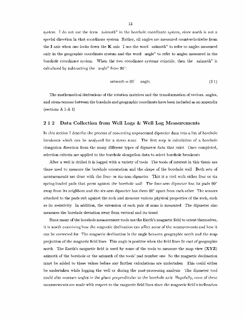
system I do not use the term azimuth in the borehole coordinate system since north is not a
special direction in that coordinate system Rather all angles are measured counterclockwise from
the I axis when one looks down the K axis I use the word azimuth to refer to angles measured
only in the geographic coordinate system and the word angle to refer to angles measured in the
borehole coordinate system When the two coordinate systems coincide then the azimuth is
calculated by subtracting the angle from
azimuth angle
The mathematical derivations of the rotation matrices and the transformation of vectors angles
and stress tensors between the borehole and geographic coordinate have been included as an appendix
sections AA
Data Collection from Well Logs Well Log Measurements
In this section I describe the process of converting unprocessed dipmeter data into a list of borehole
breakouts which can be analyzed for a stress state The rst step is calculation of a borehole
elongation direction from the many di erent types of dipmeter data that exist Once completed
selection criteria are applied to the borehole elongation data to select borehole breakouts
After a well is drilled it is logged with a variety of tools The tools of interest in this thesis are
those used to measure the borehole orientation and the shape of the borehole wall Both sets of
measurements are done with the four or sixarm dipmeter This is a tool with either four or six
springloaded pads that press against the borehole wall The fourarm dipmeter has its pads
away from its neighbors and the sixarm dipmeter has them apart from each other The sensors
attached to the pads rub against the rock and measure various physical properties of the rock such
as its resistivity In addition the extension of each pair of arms is measured The dipmeter also
measures the borehole deviation away from vertical and its trend
Since many of the borehole measurement tools use the Earths magnetic eld to orient themselves
it is worth examining how the magnetic declination can a ect some of the measurements and how it
can be corrected for The magnetic declination is the angle between geographic north and the map
projection of the magnetic eld lines This angle is positive when the eld lines lie east of geographic
north The Earths magnetic eld is used by some of the tools to measure the map view XYZ
azimuth of the borehole or the azimuth of the tools pad number one So the magnetic declination
must be added to these values before any further calculations are undertaken This could either
be undertaken while logging the well or during the postprocessing analysis The dipmeter tool
could also measure angles in the plane perpendicular to the borehole axis Hopefully none of these
measurements are made with respect to the magnetic eld lines since the magnetic elds inclination
would also have to be taken into account
The di erent borehole measurements can be grouped into two di erent sets One set of measure
ments are taken in the geographic reference frame and the other are taken in a borehole reference
frame Measurements typically taken in the borehole coordinate system are various diameters of the
hole as measured in a plane perpendicular to the borehole axis by the four or sixarm dipmeter
and the angular distance between the highest point of the borehole wall and one of the caliper arms
Measurements taken in the geographic reference frame include the azimuth of the borehole and its
deviation away from vertical
Between all of these di erent measurements three nal quantities are desired as a function of
depth These are the trend or azimuth of the borehole the borehole deviation away from vertical
and the borehole elongation angle With these three values as a function of depth the complete
stress tensor can be constrained given sucient variation in borehole orientations
Calculation of Elongation IJK Angles
Calculation of the elongation direction for a fourarm dipmeter is straightforward I assume that
the dipmeter is centered in the borehole so the elongation direction is parallel to the direction of
the longer caliper arm See Section for a discussion of the basis for this assumption I also
make the assumption that the breakout is symmetric about so that all elongation orientations
lie between and without any loss of generality
The sixarm dipmeter is similar to the fourarm dipmeter except that it has two extra arms and
all of the arms are separated by intervals Calculation of the borehole elongation direction from
a sixarm dipmeter is more complicated since it is not as obvious that any one set of caliper arms
will be aligned with the breakout In addition the extra two pads on the borehole wall may change
the threshold of detection of breakouts because the increased friction on the borehole wall requires
less ellipticity to counteract tool torque see Section I am not aware of any study in which the
breakout directions calculated from a sixarm dipmeter have been compared to those found either
from a borehole televiewer tool or from a fourarm dipmeter
Here I describe two methods of calculating the elongation direction from sixarm dipmeter data
The rst method uses the orientation of the longest caliper arm as the elongation direction However
the longest caliper arm may not track the breakout so the second method which I use on our data
ts an ellipse to the caliper arm data and takes the orientation of the semimajor axis as the elongation
direction
I briey describe the second method here The sixarm dipmeter measures three independent
diameters that are separated by These three values dene three vectors which originate at
the origin of a suitable coordinate system and are separated by intervals I assume that the
three vectors constrain an ellipse centered at the origin of the coordinate system I parameterize

Caliperarm #1
Caliperarm #2
Caliperarm #3
θX
Y
X’Y’
Boreholewall
Breakout
Breakout
Figure Geometry of the caliper arms in the sixarm dipmeter looking down onto the tool andellipse used to nd the breakout orientation
the orientation of this ellipse using the angle between the semimajor axis of the ellipse and the
direction of caliper arm Figure To determine I write three equations describing the ellipse
inserting the vector positions of the endpoints of the caliper arms The three equations are then
written in matrix form As in many linear algebra problems for a solution to exist the determinant
of the matrix must be zero Here the matrix will have zero determinant when the angle of rotation of
the ellipse is found Once this angle of rotation is found the lengths of the semimajor and semiminor
axes are easily calculated Using this information with the rotation angle allows calculation of the
elongation direction with respect to the azimuth of pad
One potential problem with this method is that the three caliper arm vectors might dene a
hyperbola instead of an ellipse This problem occurred with some of the data from Point Pedernales
and I choose to not select any breakouts where this happens
The mathematical details of this technique are as follows
I start o by dening two coordinate systems that share the same origin The rst unprimed
coordinate system XY is oriented such that its X axis is aligned with caliper arm number Since
the caliper arms are numbered clockwise caliper arm number is away from the X axis and in
the lower right quadrant The third caliper arm is away from the rst caliper arm and lies in
the lower left quadrant The second primed reference frame XY is dened to be the coordinate
system in which the equation for the ellipse can be written as
ax ay
a
that is the X and Y axes coincide with the semimajor and semiminor axes of the ellipse The

coordinates of a point in the two coordinate systems are related by the transformation
x x cos y sin
y x sin y cos
where theta is the counterclockwise angle measured from the X to the X axis in the XY coordinate
system The equation for the ellipse in unprimed coordinates is
ax cos y sin ax sin y cos a
Now one must dene the vectors representing the three caliper arms and enter them into
If the lengths of the caliper arms are c c and c respectively then
x c T
x c cos c sin T
x c cos c sin T
Three independent equations are obtained when the caliper arm vectors are substituted into
ac cos ac sin
a
ac cos cos c sin sin ac cos sin c sin cos
a
ac cos cos c sin sin ac cos sin c sin cos
a
The equations can be expressed in matrix form
BBB
c cos c sin
c cos cos c sin sin c cos sin c sin cos
c cos cos c sin sin c cos sin c sin cos
CCCA
BBB
a
a
a
CCCA
BBB
CCCA
BBB
c cos c sin
c cos c sin
c cos c sin
CCCA
BBB
a
a
a
CCCA
BBB
CCCA
M a
For to be satised the determinant of M must be This condition constrains so the
XY coordinate system has now been dened To numerically nd the NewtonRaphson method
for nding roots of functions can be applied to the determinant The angle is not unique since an

extra rotation of will just switch a and a
The semimajor and semiminor axis lengths and the ellipticity are determined by the constants
a a and a I now use the equation of the ellipse with the caliper arm locations as expressed in
the XY coordinate system
x c cos c sin T
x c cos c sin T
x c cos c sin T
I again write three equations
ax ay
a
ac cos ac sin
a
ac cos cos c sin sin ac cos sin c sin cos
a
Written in matrix form the equations become
BBB
x y
c cos c sin
c cos cos c sin sin c cos sin c sin cos
CCCA
BBB
a
a
a
CCCA
BBB
CCCA
BBB
x y
c cos c sin
c cos c sin
CCCA
BBB
a
a
a
CCCA
BBB
CCCA
N a
The determinant ofNmust be zero for to be satised This results in the following equation
dening the lengths of the semimajor and semiminor axes
c sin c sin
x c cos c cos
y cc sin sin
Equation can be rewritten in standard elliptical form
c sin c sin
cc sin sin
x c cos
c cos
cc sin sin
y
x
l
y
l
So the semimajor and semiminor axes lengths are known along with the angle The breakout

direction is therefore either degrees away from caliper arm number one if l l or degrees
away if l l
Equation fails if n In this case caliper arm number can be used instead of
caliper arm number in equation
BBB
x y
c cos c sin
c cos c sin
CCCA
BBB
a
a
a
CCCA
BBB
CCCA
Calculating the determinant of the above matrix and setting it to I nd
c sin c sin
x c cos c cos
y cc sin sin
This results in the following equation for the ellipse
c sin c sin
cc sin sin
x c cos
c cos
cc sin sin
y
Calculation of Borehole and Elongation XYZ Azimuths
In some cases it may be necessary to calculate the borehole and elongation XYZ azimuths The
borehole azimuth may need to be calculated if for some reason the well log does not list the borehole
azimuth The only method that does not involve using angles measured with respect to the Earths
magnetic eld in the borehole coordinate system is to subtract the XYZ relative bearing from the
XYZ pad number one azimuth This orientation then points at the high side of the hole which is
in the same direction as the XYZ borehole azimuth
While most of the work in this thesis uses just the borehole elongation or breakout angle in the
borehole coordinate system notably for the stress state inversion calculation the elongation direction
as projected to the horizontal is used for illustration purposes such as in the lower hemisphere
stereographic projection plots
There are three di erent methods for calculating the XYZ breakout azimuth They all rely on
the knowledge of the borehole azimuth The di erent methods are
Take the IJK relative bearing to nd the IJK angle of pad number one Find the
breakout orientation with respect to pad number one using the caliper arm length logs and get the
IJK angle of the breakout Convert this IJK angle into aXYZ azimuth using the equations derived
in Section A
Take the XYZ azimuth of pad number one convert it into an angle in the borehole

frame Section A nd the breakout angle using the caliper distances and move this angle into
the geographic reference frame
Use the XYZ relative bearing to nd the XYZ azimuth of pad number one Then go
through the same steps as in above
With these di erent methods it should be possible to calculate the breakout azimuth using any
kind of well log
Statistics of Angular Data
Various statistics of borehole breakout data are calculated throughout this work For example
the mean and standard deviation of the IJK breakout angle over a particular depth range is used
throughout the borehole breakout selection scheme The statistical techniques appropriate for linear
data are not always appropriate for circular or angular data For example consider two rays aligned
and away from the X axis Intuitively we expect the average ray to lie directly on the X
axis with a standard deviation somewhere around Calculating the mean using a linear approach
however would yield an average orientation of the ray to be One solution to this problem is to
translate all of the measurements by perform the mean calculation and then translate the result
back by This would give us the correct mean of However there are more complicated data
sets for which there is no unique translation of the coordinate system that will give a satisfactory
answer
A more general solution to the problem follows the one described by Mardia with minor
di erences which will be outlined below A complete derivation of the results from Mardia
will not be presented here just the major results First I present the results from circular two
dimensional data
Let the angles n represent n measurements Let each measurement have an associated
weight wi The weight wi can represent any associated weight of the measurement such as the
number of measurements at the particular angle or the error associated in the measurement of that
angle The mean direction of n is dened as the angle that the weighted sum of the vectors
makes with the X axis This vector sum is represented by C S where
C
Pwi cos iP
wi
S
Pwi sin iP
wi
Dene R as
R
qC S

The mean angle satises the equations
C R cos
S R sin
and can be calculated using the arctan function It can be shown that this denition of has some
useful properties First of all if the angles n are uniformly rotated by an angle then
will experience the same amount of rotation Secondly
Xwi sin i
This is equivalent to the expression Xwixi x
for the linear case
Mardia introduces a term called the dispersion D which measures the amount of disper
sion between a list of angles and a given angle The dispersion is dened as
D
Pwi cos i P
wi
The dispersion D is minimized when This can be shown by setting the derivative of equa
tion to Xwi sin i
This is equivalent to equation when is equal to
I dene a new value the circular variance as
S R
Since the range of R is from to the circular variance also ranges from to If the angular
measurements cluster then R will be near and S will be near One would like to relate the
circular variance to a linear standard deviation Mardia derives an appropriate transformation
of the circular variance from the range to a linear standard deviation on the range as
so p ln S
pnn
Mardia does not include thepnn term in the calculation of s I do so to represent
the fact that one degree of freedom is lost from the data when the mean is calculated This term

is intuitive if one thinks of making one measurement and attempting to calculate the mean and
standard deviation The mean of a sample of one is just the measurement itself However one
would have no idea of the quality of the measurement so it would be assigned a standard deviation
of The termpnn gives if there is only one measurement
All of the discussion above applies to directed angular data I also have undirected data such as
borehole breakout direction data which I assume has a symmetry There might be other data
types that have a symmetry For this reason I discuss the statistics of data with l symmetry
The appropriate transformation of this data is to increase the angular range from l to
using
l
One can then nd the mean direction
and the circular variance S of the transformed data
It can be shown that the mean circular variance and standard deviation of the original data are
related to the mean and the circular variance of the transformed data by the following equations
Mardia
l
S S
l
s p ln S
pnn l
Identication of Breakouts
Here we discuss criteria for identication of breakouts and calculation of breakout azimuths given
either oriented four or sixarm caliper data Oriented four or sixarm caliper data are measured on
a variety of di erent welllogging tools such as lowangle dipmeters highangle dipmeters formation
microscannersmicroimagers and stratigraphic highresolution dipmeter tools SHDTs
Plumb and Hickman examined the validity of using fourarm dipmeters to identify borehole
breakouts They logged a well in Auburn New York twice with a fourarm dipmeter and once with a
borehole televiewer The borehole televiewer is an acoustic logging tool that provides highresolution
information about borehole elongation and the distribution of natural fractures in wells Zemanek
et al The acoustic transit time can be used to construct detailed borehole cross sections
By comparing the orientation of breakouts from the fourarm dipmeter with borehole cross sections
constructed from the televiewer data they found that the fourarm dipmeters generally had their
long axes aligned with the breakouts This is a critical observation since borehole televiewer logs
are not commonly run in most drill holes and many wells logged with fourarm dipmeters lack the

Breakout Key Seat
Washout1
2
3
4
1
BitSize
BitSize
1
1
Increasing Caliper Distance
Caliper Arms 1−3Caliper Arms 2−4
In−Gauge Hole
(a)
(b)
(c)
(d)
Figure Examples of fourarm dipmeter caliper logs and common interpretations of boreholegeometry Caliper arms and caliper arms indicate the borehole diameter as measured betweenopposing dipmeter arms a An ingauge hole b The geometry resulting from stressinducedborehole breakouts c A minor washout with superimposed elongation d A key seat wherethe dipmeter is not centered in the borehole resulting in one caliper reading being less than the bitsize Increasing caliper arm distances are to the left Figure after Plumb and Hickman
more detailed televiewer observations
Plumb and Hickman dened ve criteria they used to identify zones of breakouts from
fourarm dipmeter logs
The tool rotation stops in the zone of elongation
The caliper arm di erence is greater than cm
The smaller of the caliper readings is close to bit size or if the smaller caliper reading is
greater than bit size it should exhibit less variation than the larger caliper
The length of the breakout zone is greater than cm
The direction of elongation should not consistently coincide with the azimuth of the high
side of the borehole when the hole deviates from vertical
These criteria attempt to eliminate some commonly observed complications in borehole shape
Figure The rst two criteria relate to rotation of the dipmeter due to cable torque as the tool is
winched up the hole The rst criterion requires the dipmeter to track the breakout and the second
deals with the observation that a cm borehole elongation was sucient to stop tool rotation for
Plumb and Hickmans winch and cable setup The third criterion eliminates positions where
the dipmeter is not centered in the borehole or where the borehole has been washedout The fourth
criterion addresses the fact that breakouts shorter than the length of the caliper pads cannot be

measured the dipmeter used by Plumb and Hickman had a pad length of cm The last
criterion addresses cable and tool drag on the borehole wall when the hole is not vertical The cable
or other tools previously used in the hole can scrape the wall and create a channel on the low side
of the hole tool marks or key seats yielding a roughly elliptical borehole shape that could be
interpreted as a breakout if only fourarm caliper data were available
From our experience with examining deviated boreholes we have slightly modied Plumb and
Hickmans breakout selection criteria The new criteria used are as follows
The tool rotation stops in the zone of elongation Dipmeter logs record either pad
azimuth or the relative bearing of pad or both The pad azimuth is the XYZ azimuth of the
number dipmeter pad The relative bearing is the IJK angle between the high side of the hole
and pad number Both of these measure the orientation of the tool in the hole Our selection
criterion for nondigital data sets is that the maximum variation of either measurement should be less
than When digital data are available the standard deviation of either data type must be less
than We use Mardias work in the statistics of angular data to calculate the average
borehole elongation direction and its standard deviation for a particular section of hole
The largest and smallest caliper arms should be at least di erent from each other
The smallest caliper arm should be larger than or equal to the bit size and smaller than
times the bit size
The standard deviation of each caliper arm over a breakout interval should be less than
cm inch
The length of the breakout zone should be at least m
The maximum di erence between the bit size and the largest caliper arm should be
cm inches
Criterion of Plumb and Hickman was tightened to be more quantitative regarding the
variation in the quality of the breakout direction Criterion was changed to demand a di erence
between the caliper arms instead of a cm di erence This criterion is more exible for boreholes
of di erent radii Criterion was slightly changed to state that the smallest caliper arm is always
as large as the bit size and no larger than times the bit size The minimum breakout length of
criterion was increased to m to nd longer more consistent breakout intervals Criterion of
Plumb and Hickman discards breakouts that t all other selection criteria but are parallel to the
high and low sides of the hole We keep such data initially since the theoretical breakout patterns
for most stress regimes Figure show that in certain borehole orientations the breakouts are
expected to be aligned with the high and low side of the hole After initial data analysis if we
determine that some of these elongation directions are probably due to key seats we remove them
manually from the data set We also note that Qian and Pedersen performed an inversion of
a set of breakouts measured with fourarm dipmeter data containing radial breakouts Figure

Finally we add one more criterion which discards breakouts with very large spalled regions since
other processes such as wholesale failure along fault zones might account for large spalled regions
Propagation of Errors
As with any study the propagation of errors through the data analysis should be studied Here the
errors involved in measuring the borehole diameters will rst be considered followed by consideration
of the angular measurements which prove to be more important
There are two main sources of error to consider The rst is systematic errors associated with the
logging equipment This is sometimes compensated for at the well site by taking extra measurements
that are used while logging the well Examples of this are calibration measurements for the caliper
arms and declination measurements to correctly orient the tool in the hole The other source of
errors is in the digitization of paper well logs if digital data are not available Digitization errors can
result in apparent misalignment between di erent measurements such as caliper one and caliper
two showing the start of a washout at di erent depths Also the magnitude of the washout could
be digitized poorly showing that the washout is not as large as it actually is
The error of measuring the borehole diameter with a fourarm caliper does not weigh too heavily
in calculating the borehole breakout direction Since the breakout direction is assumed parallel to
the more extended caliper arms only a comparison between caliper arm and caliper arm must
be made If caliper arms and are equal within the errors of the measurements the breakout
direction would be unconstrained but the data would not be used since it does not meet Plumb and
Hickmans criteria specically and
The case of a sixarm caliper is harder since the breakout direction depends strongly on the
caliper arm lengths However much of our data is from fourarm calipers in this study so this is
not too important
The most important source of errors is from angular measurements particularly in calculating
the breakout azimuth map view XYZ These errors are magnied when the borehole is highly
deviated which is an important point considering that the objective of this work is to analyze very
deviated boreholes
Consider a breakout direction angle measured by the pad number one azimuth in the borehole
IJK reference frame where the borehole is deviated by The borehole angle lies in a circle
perpendicular to the borehole axis This circle becomes an ellipse with a large ellipticity when
projected to the horizontal This means that unless the IJK angle points in the high or low side of
the hole it will be rotated such that the breakout orientation Figure appears more azimuthal
than radial This has important consequences for a thrust faulting regime where the breakout
pattern is expected to be radial Figure
This can be easily visualized in a plot of the XYZ breakout azimuth for a variety of IJK

0.0 90.0 180.0 270.0 360.0IJK breakout angle (degrees)
–180.0
–90.0
0.0
90.0
180.0
XY
Z b
reak
out a
zim
uth
(deg
rees
)
Figure Plot of the XYZ breakout azimuth against the IJK breakout angle for a deviatednorth plunging well Note that any errors in the IJK angle are magnied when the angle lies near and angles which correspond to a breakout at the high and low side of the hole
breakout angles for a deviated borehole plunging due north Figure An IJK breakout
angle of represents the high side of the hole and an angle of points at the low side of the
hole Notice that any error in the angular measurement itself or in the digitization is magnied
here For example if the breakout was on the high side of the hole but digitization error put
the angle at then the XYZ angle is roughly times greater than the error in the borehole
coordinate system
In light of this then eld measurements showing consistent nonazimuthally trending breakout
orientations should be evaluated carefully
Inverting the Breakout Data
In this section I describe the steps taken after a dipmeter data set is gathered to determine the stress
state that best describes the data Briey the steps are
Calculate the IJK elongation angle for all wells at m depth spacing
Use the breakout selection criteria listed above to identify breakouts
Optionally bin the breakouts into bins of XYZ borehole azimuth and borehole deviation
I calculate a weighted average breakout direction and a weighted standard deviation of the breakout
angles Mardia The individual breakouts are weighted linearly with their length and inversely
with the standard deviation of the breakout angle over the breakouts length
Use a genetic algorithm GA to identify the region of the stress state solution space that

N
S
EW
Figure A lower hemisphere stereographic projection showing the grid used to bin the boreholebreakout data Each bin has an area equivalent to a x bin at the center of the projections
most likely contains the minimum weighted onenorm mist between a stress state and the possibly
binned breakout data
Run a Ndimensional optimizer with the results from the GA to nd the minimummist
Calculate error bounds on the best tting stress state
Binning of Breakout Data
Much of the borehole breakout data I have examined is very scattered both in the orientation of
breakouts and in the orientations of the boreholes in a particular eld of study ie Figure
The data might also show a large group of breakouts at one borehole orientation and a few scattered
breakouts in others I would like the few scattered breakouts to have a comparable weight for the
optimization as the group of more numerous breakouts since the variation of borehole orientations
is equally as important to our optimization as the quantity of breakouts
For these reasons I may bin the borehole breakout data into equalarea stereographic area bins
These bins are equivalent in size to a x bin located at the center of a stereographic projection
Figure
To arrive at an IJK borehole breakout orientation for each bin I use the statistics of angular data
as described in Section weighting the mean breakout direction linearly with the breakouts
length and inversely by the square of the standard deviation of the breakout orientation
wj ljj

Here wj is the weighting factor appearing in equations and aj is the IJK angle
of the jth breakout lj is its length and j is the standard deviation of the IJK breakout angle
Calculation of the mean breakout angle in this manner favors longer breakouts with smaller variations
in the breakout angle To calculate the mean and standard deviation of nonangular measurements
associated with each breakout I use the following equations Bevington
x
PwjxjPwj
x NPwjxj x
N P
wj
Euler Angle Description of a Stress State
A stress tensor can be described in a number of ways I would like a parameterization of the stress
tensor that separates the magnitudes of the principal stresses from the orientation of the principal
stress directions
I choose to parameterize the stress state with four parameters three Euler angles and the stress
state ratio equation The three Euler angles describe three successive rotations about various
coordinate axes and are a natural representation often used to completely describe the orientation
of a set of axes attached to a body in space Goldstein I use this formalism to describe the
orientation of the eigenvectors of a stress tensor
Since the stress tensor is completely described by six parameters and three of the parameters
describe the stress state orientation the two parameters I am not constraining describe the magni
tudes of the principal stresses I can parameterize the magnitudes of the principal stress directions
as
S ab
S ab
S ab
where is the ratio previously dened equation and a and b are unknown constants Exami
nation of equations through shows that the location of the axis of greatest compressive
stress tmax is una ected by the constant multiplicative factor a in equations The
remaining parameter b does e ect the position of tmax and tmin However I choose to ignore b
in the parameterization of the stress state by setting it equal to
To describe the arbitrary orientation of a body with Euler angles the angles must be allowed

to vary from to However since a rotation of a stress tensor by leaves the stress tensor
invariant the Euler angles can be limited to The largest problem with this parameterization
is when the amount of the second rotation is In this case the rst and third rotations rotate the
coordinate system about the same axis leading to multiple parameterizations that describe the same
eigenvector orientations
Theoretical Breakout Directions in Arbitrary Stress Fields
Here we discuss how the theoretical breakout direction is calculated given an arbitrary borehole
orientation and fareld stress state First the fareld tectonic stress is transformed or rotated into
the coordinate system associated with the borehole as the stress tensor
SIJK
BBB
Sii Sij Ski
Sij Sjj Sjk
Ski Sjk Skk
CCCA
with compressional stress positive
Hiramatsu and Oka and Fairhurst derived the relationship between fareld stresses
and stresses on the wall of a cylindrical hole assuming that the medium is isotropic homogeneous
and linearly elastic with constant uid pressure in the borehole The stresses on the borehole wall
in the borehole coordinate system are given by
kk Skk Sii Sjj cos Sij sin
Sii Sjj Sii Sjj cos Sij sin !P
k Sjk cos Ski sin
rr !P
where !P is the di erence between the borehole uid pressure and the in situ pore pressure is
Poissons ratio of the rock and is taken to be Throughout this work !P is taken to be The
angle is measured from the I axis toward the J axis The K axis in the rK coordinate system is
the same K axis in the IJK coordinate system Figure Note that the form of equations
is di erent from that of equations appearing in Mastin equations A and A Qian
and Pedersen equation and Peska and Zoback equation A Mastin and
Qian and Pedersen contain errors in the denition of kk and Peska and Zoback s
increases in a clockwise sense while the appearing in equations increases in
a counterclockwise sense

IJ
K
α
αασ
Sii
Ski
Sij
Ski
Skk
Sjk
Sij
Sjk
Sjj
σkk
τ αk
σrr
Figure View of the borehole and the components of the stress tensor in the borehole coordinatesystem The angle is used in nding the cylindrical components of the stress tensor on the boreholewall After Mastin
The principal stresses at any given point on the borehole wall are
tmax
kk
qkk k
tmin
kk
qkk k
rr !P
where tmax and tmin are the maximum and minimum principal stresses in the plane tangential
to the borehole wall The location of the maximum and minimum values of the tangential principal
stresses dene the location of borehole breakouts and tensile fractures if the rock strength is exceeded
borehole breakouts occur where tmax is a maximum and tensile fractures occur where tmin is
minimized Peska and Zoback The easiest way to obtain the angles where tmax is maximized
and tmin is minimized given the square root term in the denition of tmax and tmin is to use
Brents computational method which does not rely upon rst derivative information of the function
being optimized Brent Press et al
Selection and Calculation of a Mist Measure
Optimization of a model from data requires a mist measure that describes how well a particular
model ts the observed data A class of mist measures is based on the p norm Parker and McNutt
p
nX
j
j ojj
pA
p

where j is a theoretical value for an observation oj and j is the measure of error in the observation
Di erent values of p lead to di erent weightings of outlying data For example the uniform norm
minimizes the largest di erence between an observed and modeled value The familiar
mist measure is recognized as In the same manner that the p norm is strongly
inuenced by extreme and outlier data Parker and McNutt raise the same criticism about
the measure Parker and McNutt suggest a onenorm mist measure p
M
nXj
j j oj j
j
and derive the statistics ie the mean variance and condence tables associated with the one
norm measure Gephart and Forsyth use the onenorm mist to determine the stress state
from earthquake focal mechanism data
In addition to testing to determine which order of p to use in the mist measure two di erent
mist calculations are introduced here The rst mist calculation sums the angular di erence
between the predicted and observed breakout location on the borehole wall
m
nXj
lj
oj mj S
j
where lj is the length of the jth breakout oj is the breakout IJK angle mj S is the IJK angle
of the predicted location of the breakout on the borehole wall for a given stress state S and j is
the standard deviation of the IJK breakout angle for a single breakout or the standard deviation of
the IJK breakout angles from binned breakouts
The second mist measure sums the di erence between tmax equation at the angle of the
breakout and tmax at the predicted location of the breakout on the borehole wall A rst attempt
at creating a mist measure using a stress di erence is
nXj
ljtmax
mj S tmax
oj
Sdmaxo
jj
ojjjtmax tmaxoj j
The two factors in the denominator of the stress mist measure need some explanation The term
Sd is the maximum value of the di erence between the maximum and minimum values of tmax
on the borehole wall for a particular borehole orientation and is maximized when the borehole is
oriented parallel to the S axis If the principal stresses S S and S are aligned with Sii Sjj
and Skk respectively then from equations
Sd tmax
tmax
S S

j S S Sj
j S S Sj
The Sd term is introduced so that the stress mist for di erent breakouts are weighted evenly even if
the stress model for the breakout data imposes di erent stress states at di erent borehole breakout
locations otherwise a mist measure without the Sd term would weight deeper breakouts more
than shallow breakouts if a depth dependent stress model is used
The second term in the denominator
maxo
jjo
jjjtmax tmax
oj j
tries to serve as a measure of the standard deviation of tmax in the same sense that j measures the
standard deviation of oj This term calculates the maximum change in tmax as varies between
oj j and oj j Two problems with this term prevent its use in calculating m First
there are borehole orientations where tmax does not change with leading to a denominator equal
to or close to Secondly calculating the term is computationally infeasible since tmax is itself a
function of the stress state For these reasons the IJK breakout angle is used to weigh the stress
mist and m is dened as
m
nXj
ljtmax
mj S tmax
oj
Sdj
The stress mist measure m has some properties that make it a better mist measure than
the angular mist measure m First breakouts occur at orientations where the rock strength is
exceeded by the stresses at the borehole wall and hence stresses are the natural measure of mist
between model and observation Secondly the angular di erence between predicted and observed
breakout orientations do not accurately represent the mist between observation and data For
certain borehole orientations where tmax around the borehole is constant breakouts if they occur
may occur at almost any orientation Figure The angular mist measure for these breakouts
will articially inate the mist measure These breakouts will not contribute signicantly to the
stress mist measure because at these borehole orientations tmax is constant or nearly constant
Stress inversion results from a onenorm angular inversion equation a onenorm stress
di erence inversion equation and a stress di erence inversion with
m
nXj
ljSd
tmax
mj S tmax
oj
j
are now compared Figures The data used to perform the comparisons are from Cook Inlet

Table Comparison of stress state inversion results using three di erent mist measures
S S S S S SMist measure Azi Dev Azi Dev Azi Dev Onenorm angular di erence
Onenorm stress di erence
Twonorm stress di erence
The data used to perform the comparisons are from Cook Inlet Alaska and are composed of nonradial borehole breakouts identied from all of the wells except Gp and Smgs see Chapter
Alaska and are composed of nonradial borehole breakouts identied from all of the wells except
Gp and Smgs see Chapter Nonradial breakouts are those breakouts where the IJK breakout
angle is at least away from the highside of the hole The two stress di erence inversions the
rst using a onenorm mist measure and the second using a mist measure show very similar
results Table Figures and Except for the onenorm value of the principal
stress directions and the values from both mist measure solutions occur in the other solutions
condence region Given the similarity of the two solutions for a complicated breakout data
set only the onenorm mist measure is used in all subsequent inversions
The onenorm stress di erence mist measure and the onenorm angular di erence mist inver
sions have substantially di erent stress state and value results Table Figures and
The angular inversion identied an oblique normal faulting stress state with The
stress state is oriented such that breakouts observed in the more highly deviated southward plunging
boreholes are satisfactorily t The stress di erence inversion results found an almost degenerate
thrust faulting stress state with Unlike the angular di erence inversion results the
stress di erence inversion results have much smaller condence limits particularly on the value
The smaller condence regions are probably due to less accumulated mist when highly vari
ably oriented borehole breakouts are included in the mist calculations In these cases the stress
di erence mist can stay small if it places a nodal point near variably oriented breakout data while
the angular di erence mist always accumulates a larger mist for variably oriented data
A similar comparison of inversion results from the angular di erence mist measure m and the
stress di erence mist measure m are performed on the Qian and Pedersen Chapter
and the Cook Inlet Alaska Chapter data sets Unlike the borehole breakout data used in the
above comparison these two data sets are much smaller more internally consistent and occupy less
of the borehole orientation space In these cases the angular and stress di erence inversion results
were very similar The principal di erence between the sets of inversion results are the smaller
condence regions identied in the stress di erence inversion

N
S
EW
75.0-3031.6
-614.9
N
S
EW
75.0-3031.6
-614.9N
S
EW
75.0-3031.6
-614.9
Figure Comparison of stress state inversion results using three di erent mist measures topResults using a onenorm angular di erence measure bottom left Results using a onenorm stressdi erence measure bottom right Results using a stress di erence measure Lower hemispherestereographic projection of nonradial identied breakouts from all available wells excluding thebreakouts from wells Gp and Smgs in Cook Inlet Alaska see Chapter plotted on top of thetheoretical breakout pattern of a best tting stress state Nonradial breakouts are those breakoutswhere the IJK breakout angle is at least away from the highside of the hole The graduatedscale shows the depth of the selected breakouts in meters Solid circles are nodal points at whichthe stress anisotropy is zero corresponding to borehole orientations with no preferred breakoutdirection Width of the breakout azimuth line is proportional to the breakout length divided by thestandard deviation of the IJK breakout angle over the length of the breakout

0
1
2
3
4
5
6
7
8
9
10
Num
ber
of b
reak
outs
-90 -75 -60 -45 -30 -15 0 15 30 45 60 75 90
Angular difference (degrees)
0
5
10
15
20
25
30
35
Num
ber
of b
reak
outs
0.0 0.1 0.2 0.3 0.4 0.5
Stress difference
0
5
10
15
20
25
30
35
Num
ber
of b
reak
outs
0.0 0.1 0.2 0.3 0.4 0.5
Stress difference
Figure Histograms of residuals between the borehole breakout data plotted in Figure andthe best tting stress state for a particular mist measure top Histogram of the residual angular di erence oj mj S in
bins using the onenorm angular mist measure inversion resultsbottom left Histogram of the residual stress di erence tmax
mj S tmax
oj Sd between
the theoretical tmax at the predicted location of the breakout and tmax at the breakout usingthe onenorm stress di erence measure bottom right Histogram of the residual stress di erencetmax
mj S tmax
oj Sd between the theoretical tmax at the predicted location of the
breakout and tmax at the breakout using the stress di erence measure

22
24
26
28
30
32
34
36
38
40
42
One
-nor
m A
ngul
ar M
isfit
0.0 0.2 0.4 0.6 0.8 1.0
Stress Ratio φ
22
24
26
28
30
32
34
36
38
40
42
One
-nor
m A
ngul
ar M
isfit
0.0 0.2 0.4 0.6 0.8 1.0
Stress Ratio φ
22
24
26
28
30
32
34
36
38
40
42
One
-nor
m A
ngul
ar M
isfit
0.0 0.2 0.4 0.6 0.8 1.0
Stress Ratio φ
0.0
0.1
0.2
0.3
0.4
One
-nor
m S
tres
s M
isfit
0.0 0.2 0.4 0.6 0.8 1.0
Stress Ratio φ
0.0
0.1
0.2
0.3
0.4
One
-nor
m S
tres
s M
isfit
0.0 0.2 0.4 0.6 0.8 1.0
Stress Ratio φ
0.0
0.1
0.2
0.3
0.4
One
-nor
m S
tres
s M
isfit
0.0 0.2 0.4 0.6 0.8 1.0
Stress Ratio φ0
20000
40000
60000
80000
100000
120000
χ2 S
tres
s M
isfit
0.0 0.2 0.4 0.6 0.8 1.0
Stress Ratio φ
0
20000
40000
60000
80000
100000
120000
χ2 S
tres
s M
isfit
0.0 0.2 0.4 0.6 0.8 1.0
Stress Ratio φ
0
20000
40000
60000
80000
100000
120000
χ2 S
tres
s M
isfit
0.0 0.2 0.4 0.6 0.8 1.0
Stress Ratio φ
Figure Various weighted mist measures plotted as a function of for the borehole breakoutdata shown in Figure where the thick solid line is the condence limit for the inversion thethin solid line is the minimized mist where for each value of the directions of the principal stressaxes are allowed to vary so that the minimum mist is obtained and the dotted line is the mistusing the principal stress directions from the respective best tting model The condencevalue is plotted at the constant solid line top Onenorm angular di erence mists bottom leftOnenorm stress di erence mists bottom right stress di erence mists

0˚
315˚
270˚
225˚
180˚
135˚
90˚
45˚
1
23
1
23
1
23
0˚
315˚
270˚
225˚
180˚
135˚
90˚
45˚
1
23
1
23
1
23
0˚
315˚
270˚
225˚
180˚
135˚
90˚
45˚
1
23
1
23
1
23
Figure Comparison of stress state inversion results using three di erent mist measures topResults using a onenorm angular di erence measure bottom left Results using a onenorm stressdi erence measure bottom right Results using a stress di erence measure Lower hemispherestereographic projection plot where the digits and show the best tting orientation of theS S and S principal stress axes for the borehole breakout data plotted in Figure The condence limits of the S S and S orientations are plotted as thick solid lines thin solid linesand dotted lines respectively

Fitting the Breakout Data
Since the determination of the best tting stress state for a set of borehole breakout data is inherently
nonlinear forward modeling is used instead of an inversion technique Inversions have been used by
others eg Qian and Pedersen A twostep forward modeling approach is used here First
a genetic algorithm or GA Holland Davis Goldberg is applied to the problem to
nd an approximate best tting stress state using the stress state parameterization described above
consisting of the variables Here the borehole azimuth and the borehole deviation
are the rst two Euler angles and is the third Euler angle A Ndimensional optimizer is then
initialized with the GAs results to nd the best tting stress state
Genetic algorithms are an attractive approach to solving hard nonlinear problems in which
the forward calculation is straightforward but more traditional techniques might fail Some of the
advantages of GAs are that they eciently search the model space do not require a good starting
model and do not get trapped in local minima unlike gradient search methods
GAs operate on a population of models Figure The models are often binary coded just as
oating point numbers are encoded in a computer An individual binaryencoded model is termed
a chromosome The rst generation of chromosomes is randomly generated Each chromosome
has associated with it an objective value which is a problemspecic measure of how well the
chromosome solves the problem From the objective value is calculated a tness value the higher
the tness the better the chromosome In this work each chromosome represents a distinct regional
stress state and the objective value is the weighted onenorm mist between the observed and
theoretical IJK breakout angles Since smaller onenorm mists correspond to higher levels of
tness we use the following equation to relate the two
fi "o o oi
o
where "o is the populations mean objective value o is the standard deviation of the objective values
oi is the ith chromosomes objective value and fi is the ith tness value Holland
After the tness values have been calculated chromosomes are randomly selected to mate to
create the next generation of chromosomes Chromosomes with higher tness values on average
mate more often Mating between two chromosomes is performed by randomly exchanging part of
the binary patterns of both parent chromosomes This operation is known as crossover Crossover
is performed only roughly of the time between two chromosomes In the other of matings
the two chromosomes are carried directly into the next generation without crossover
The nal operation of the GA is mutation whereby a small fraction of the bits of a chromosome
are ipped This process introduces variability into the population and allows broader searching of
the solution space The next generation of chromosomes has now been created and the cycle begins

See = 3
Snn = 6
Suu = 7
Sen = 1
Snu = 2
Sue = 1
0 1 1 1 1 0 1 1 1 0 0 1 0 1 0 0 0 1
Calculate the fitness of each model
Select the pairs of models to mate
Mate the models and perform crossovers
Crossover Mutation
3 1 11 6 21 2 7
Initialize the population with random parameterized models
Example: Parameterize the stress tensor S =
Parameter Representation in Genetic Algorithms
Operation of the Genetic Algorithm
Genetic Operators
Mutate the child models
Figure top Example parameterization of a stress tensor into a binary encoded chromosomemiddle Flow diagram of a genetic algorithm bottom Example of the crossover and mutationoperators on chromosomes

anew with the calculation of the populations objective values
The GAs used in this research are run with populations of several hundred chromosomes for
several hundred generations Since GAs do not guarantee that they nd the optimal solution to a
problem the particular stress state corresponding to the minimum mist observed for all of the GA
runs completed is taken as the starting point for a general Ndimensional optimizer routine The
Powell optimizer is used as described and coded by Brent This particular optimizer does
not require the use of derivatives of the function it is trying to optimize a feature that makes it
attractive for the borehole breakout problem
Experience with various breakout data sets has shown that starting the Powell optimizer with
a purely random stress state does not lead to a global minimum of the onenorm mist even for
theoretically generated breakout data The GA thus supplies an important rst step in eciently
searching the space of stress states for good starting stress states for the Powell optimizer In
practice each data set is run through GA with di erent random numbers several times to make sure
that an acceptable global onenorm mist minimum is found Even though the Powell optimizer is
used after the GA the mist is not a smooth function of the stress state since di erent GA and
Powell runs nd di erent local minima A localized GA search could be used to identify a better
tting stress state than the one the Powell search generated but such a search is not performed
because it would probably not improve the results signicantly
Condence Limits
A genetic algorithm and Powell optimization search identies the best tting stress state model for
a set of borehole breakout data The next step calculates the region of stress state space that with
a chance contains the true stress state parameter values The condence limits on the best
tting stress state are determined using a modication of Gephart and Forsyths technique for
dening condence limits on stress state determinations from focal mechanisms Condence limits
for both onenorm p and twonorm p mist measures are calculated
The rst step in calculating the condence region for a best tting model is to assume
that by performing this one experiment an experiment in the sense that oil wells were drilled and
borehole breakout orientations were measured something is known about the ensemble of mists
of the best tting models that would result if the experiment were performed innitely many times
The statistics of the mist measures gathered by performing the experiment many times over can
be calculated from the mist measure itself Relating the experimentally determined mist measure
gathered in the one performed experiment to the statistics of the distribution of mist measures
leads to the calculation of the mist measure M pP such that a certain percentage P of all
mist measures have mists less than M pP If it is known that of all of the mist measures
from these experiments have mist measures mp M p then the condence limit has

been identied
It should be stated that the distributions ofmp values calculated in searching for the best tting
model for the single experiment are not being considered In the single experiment the best tting
model has a mist mp at one end of a distribution of mists corresponding to slightly di erent
stress states Instead consider that when the best model for the experiment has been identied all
of the other possible stress states for the data in this experiment are ignored Here the distribution
of best tting models or mists that would be found if all of the boreholes were redrilled and
breakout orientations remeasured are considered
The statistics of the onenorm mist p are considered rst followed by a similar analysis
for the twonorm mist p The results of Parker and McNutt who calculated the
statistics of the onenorm mist are used here Express the onenorm mist as
m
nXj
jxj j j
where xj are independent normal random variables with zero mean and standard deviations j The
expected value of m is
m
r
n n
Parker and McNutt also wrote a program which given a probability P and n calculates
the mist M P n such that the probability is P that m M P n In other words this
program ndsM P n such that the integral from toM of the onenorm distribution is P for
a onenorm distribution of the order of n M P n is used later to calculate the condence
limit
To nd the condence limit begin by deningP
min to be the mist measure of the best
tting model Assume that this particular onenorm mist corresponds to the mean mist of a one
norm distribution Of course the mean mist and the minimized mist will di er so the assumption
is made that the errors j were incorrectly estimated To correct this estimation a new constant
factor f is introduced which multiplies all of the standard deviations j such that a new mist
sum is equal to the expected mist Since the best tting model has already been identied k
degrees of freedom have been lost where k is the number of variables in the problem Therefore
the expected onenorm mean for n k observations is used Mathematically this becomes
Xmin
nX
j
j j oj j
j
n k
nXj
j j oj j
fjfrom

Pmin
f
f
Pmin
n k
Finally to nd the P condence mist valueP
P the following expression is used
PP
fM P n k
whereM P nk is the function given by Parker and McNutt The number of parameters
identied in the genetic algorithm and Powell search k must still be subtracted from n to useM
Solving forP
PXP
MP n k
n k
Xmin
Gephart and Forsyth nd a similar expression in their equation except they assumed that
for large n one can replace the onenorm inverse cumulative function M P n with values from
standard tables of Gaussian statistics Since a code was obtained that calculates M P n there
was no reason to make this assumption
The logic that led to equation can be used to calculate the mist value for a twonorm
p mist measure Instead of using which involves the square root of the sum of mists
equation the mist measure will be used Dene m as
m nX
j
xjj
where xj are independent normal random variables with zero mean and standard deviations j The
expected value of m is
m n
DeneP
min as the minimum twonorm mist measure determined from the genetic algorithm and
Powell optimization searchXmin
nXj
j ojj
The same logic that led to equation results in the following mathematical steps
n k
nXj
j ojgj
from
Pmin
g

g
Pmin
n kPP
g M P n k
XP
M P n k
n k
Xmin
Here M P n k is the inverse probability distribution function for the distribution andPP is the mist measure that contains P percent of the mist measures for an experiment with n
observations and k modeled parameters
Condence Limits on Individual Stress State Parameters
Unlike other inversion methods the forward modeling approach does not by default give condence
limits on individual parameters of the model The condence limits on the stress state ratio are
calculated by nding the values of for which the mist measure is equal to the condence
mist value In searching for these values the principal stress directions are allowed to rotate
to minimize the mist for a particular value The condence limits on the Euler angles are not
calculated since the successive nature of the Euler angle rotations to the principal stress directions
removes any simple meaning between the Euler angle condence limits and the principal stress
direction condence limits
To calculate the condence limits on the principal stress directions the stress state ratio is
xed and the borehole azimuth is iterated from to and the borehole deviation is iterated
from to in increments This iteration rotates the J axis across the lower hemisphere of
a stereographic plot For each orientation of J within the lower hemisphere the mist measure
is minimized as a function of the third Euler angle Since there are three condence limits to
calculate Sjj is set to to identify the S condence limits Sjj is set to to identify the S
condence limits and Sjj is set to to identify the S condence limits In each of the three cases
Sii and Skk are set to the other two principal stress values The particular choice of the assignment
of Sii and Skk to the remaining two principal stress values is irrelevant once the mist measure has
been minimized as a function of the third Euler angle Contour plots of the condence limits
on the principal stress directions show smaller contour regions that are sometimes rotated away
from their minimized locations when the stress state ratio is varied away from the minimummist

Chapter Analysis of the Siljan Deep Drilling
Project Breakout Data
The intention of this chapter is to compare the Qian and Pedersen nonlinear borehole breakout
inversion technique and the genetic algorithm and Powell optimizer inversion technique developed
above by reanalyzing the borehole breakout data presented by Qian and Pedersen from the
Siljan Deep Drilling Project in Sweden The regional tectonic implications of this reanalysis will
not be examined here The borehole breakout data are taken from Table of Qian and Pedersen
and are plotted in Figure This table lists the average borehole azimuth deviation and
breakout orientation for each m depth range Also listed is the variance of the breakout direction
in degrees over that m interval No conclusions regarding the relationship between breakout
length and the insitu stress state can be gathered here because Qian and Pedersen did not
publish information on breakout length Figure plots a histogram of the angular di erence
between the location of the high side of the borehole and the breakout angle as measured in the
plane perpendicular to the borehole axis for all of the data The breakouts are clustered around
the high side of the hole and could possibly be due to tool drag However the breakout azimuth is
constant regardless of the borehole azimuth suggesting that it is unlikely that the breakouts are
caused only by tool drag
Qian and Pedersen applied a nonlinear inversion technique to their data assuming a
vertical principal stress direction with Poissons ratio equal to They found the stress state
to be a strikeslip regime SH Sv Sh with the maximum horizontal stress located
east of north The ratio of stresses was SHSv
and ShSv which corresponds to
a stress ratio varying from to with an optimal value of The error bounds listed here
are nonlinear error bounds calculated by varying the stress parameters until a large enough mist
was observed
Qian and Pedersens data are plotted in Figure with the theoretical breakout pattern
expected for the stress state resulting from their inversion A Poissons ratio of was used in this
calculation The data show almost constant breakout azimuths regardless of the borehole orientation
Because of the relatively restricted range of borehole azimuths present in this data set a large number
of nondegenerate normal and strikeslip faulting stress regimes could t these observations with
nearly constant breakout orientations up to the maximum deviation of Figure Clearly the
data are not well distributed in order to constrain the complete stress tensor Qian and Pedersens
high uncertainty in the ShSv ratio reects exactly this problem with the data distribution

N
S
EW
45.0
90.0
-6050
-1450
Figure Compiled and processed data from the Siljan Deep Drilling Project in Sweden fromQian and Pedersen plotted on top of the theoretical breakout pattern for their best ttingstress state of SHSv and ShSv where SH lies east of north Solid circles arenodal points at which the stress anisotropy is zero corresponding to borehole orientations withno preferred breakout direction The nodal points for this stress state lie at a deviation of APoissons ratio of was used to calculate the breakout pattern The vertical depth scale is inmeters
0
5
10
15
Num
ber
Bre
akou
ts
-50 0 50 100
High Side Angle - Breakout Angle
Figure Histogram of the angular di erence measured in the plane perpendicular to the boreholeaxis between the breakout orientation and the high and low sides of the borehole for the Qian and
Pedersen data

Table Characteristics of the stress state that minimized the weighted onenorm angular di erencemist of the Qian and Pedersen borehole breakout data
S S SAzimuth NE NE NEPlunge
Value
Optimized minimum weighted onenormangular di erence mist condence level forweighted onenorm angular di erence mist
Table Characteristics of the stress state that minimized the weighted onenorm stress di erencemist of the Qian and Pedersen borehole breakout data
S S SAzimuth NE NE NEPlunge
Value
Optimized minimum weighted onenormstress di erence mist condence levelfor weighted onenorm stress di erence mist
This will be a common problem in strikeslip stress regimes if highly deviated holes are not available
The only way to remedy this is to either nd or drill boreholes that are nearly horizontal
The stress inversion results presented byQian and Pedersen are now compared to the stress
inversion results generated by the genetic algorithm and Powell optimizer stress inversion technique
using both the onenorm angular di erence mist measure m equation and the onenorm
stress di erence mist measure m equation The Qian and Pedersen borehole break
out data is used unmodied the breakout selection criteria introduced above Section were
not used since the original caliper curves were not available and the data were not gridded since the
data are highly consistent
The stress inversion results using the m and m mist measures are very similar Figures
Both inversions identied a thrust faulting stress state The principal stress directions identied
using the two di erent mist measures are almost identical as shown in Figure which plots
orientations of the principal stress directions and their condence regions on a lower hemisphere
stereographic projection plot keeping constant The angular di erence inversion found a stress
state Table in which S is oriented NE plunging S is also almost horizontal oriented
NE plunging and S is almost vertical plunging at an azimuth of NE The
stress di erence inversion found a stress state Table with S oriented at an azimuth of E
plunging S oriented at an azimuth of E plunging and S oriented almost vertical
at an azimuth of E plunging The angular di erence measure identied much larger

N
S
EW
45.0
90.0
-6050
-1450N
S
EW
45.0
90.0
-6050
-1450
Figure Compiled and processed Qian and Pedersen borehole breakout data plotted ontop of the theoretical breakout pattern for a best tting stress state generated using the geneticalgorithm and Powell optimizer inversion technique Solid circles are nodal points at which thestress anisotropy is zero corresponding to borehole orientations with no preferred breakout directionA Poissons ratio of was used to calculate the breakout pattern The vertical depth scale isin meters left Theoretical breakout pattern from the onenorm angular di erence mist measureinversion right Theoretical breakout pattern from the onenorm stress di erence mist measureinversion
condence regions for the principal stress directions The principal stress directions found by the
stress di erence mist measure inversion lie within the condence region of those found by
the angular mist measure inversion The two best tting stress state ratios are substantially
di erent Figure the angular di erence mist measure found while the stress
di erence mist measure found However given that the condence limits for
the angular di erence value span the range from to the two inverted stress states may be
considered identical
The largest di erence between the two inversions is that the condence regions for the
stress di erence mist measure are much smaller than those for the angular di erence mist measure
Figure This may be due to the fact that the stress di erence inversion was able to almost
perfectly t the data m and thus any small changes to the optimum stress will very
quickly result in a larger mist value This can be seen by comparing the minimum mist identied
to the average mist of all stress states The stress di erence mist for the best tting stress state
m is times smaller than the average stress di erence mist m On
the other hand the smallest angular di erence mist m is a roughly onetenth the size of
the average angular di erence mist m So the stress di erence inversion has many fewer
stress states with associated mist values near the minimum mist than does the angular di erence

0˚
315˚
270˚
225˚
180˚
135˚
90˚
45˚
1
2
3
1
2
3
1
2
3
0˚
315˚
270˚
225˚
180˚
135˚
90˚
45˚
1
2
3
1
2
3
1
2
3
Figure Results from the reanalysis of the Qian and Pedersen borehole breakout dataLower hemisphere stereographic projection plot where the digits and show the optimizedorientation of the S S and S principal stress axes respectively The weighted onenormmist condence limits of the S S and S orientations are plotted as thick solid lines thin solidlines and dotted lines respectively left Inversion using the onenorm angular di erence mistmeasure The stress state ratio is held constant at Note that the direction of S is verywell constrained but S and S can lie virtually anywhere within a vertical plane striking N
Eright Inversion using the onenorm stress di erence mist measure is held constant at Thebest tting principal stress directions are within the condence limits identied in left gure
inversion Examination of the stress di erence condence regions for and above condence
limits show that the S and S contours extend in a NNESSW direction following the trend of the
S and S angular di erence condence limits
Aside from the principal stress directions the stress state implications of these two inversions are
quite di erent The angular di erence inversion implies that only the direction of S is constrained
and that the orientations of S and S are unconstrained about an arbitrary rotation about the S
axis Figure demonstrates that the stress ratio is unconstrained since there exists a stress
state that can be rotated in such a way to t the borehole breakout data within the condence
limits for any The stress di erence inversion identies the same stress state within the angular
di erence inversions condence limits but does not allow an arbitrary rotation of the S and
S axes about the S direction and it also tightly constrains Given that the stress di erence
inversion is more physically realistic Section and given the unconstrained nature of the
angular di erence inversion the stress di erence inversion will be used as the representative stress
state for the genetic algorithm and Powell inversion technique and will be used as a comparison
against Qian and Pedersens best tting stress state
The orientations of SH determined by Qian and Pedersen and determined here di er by
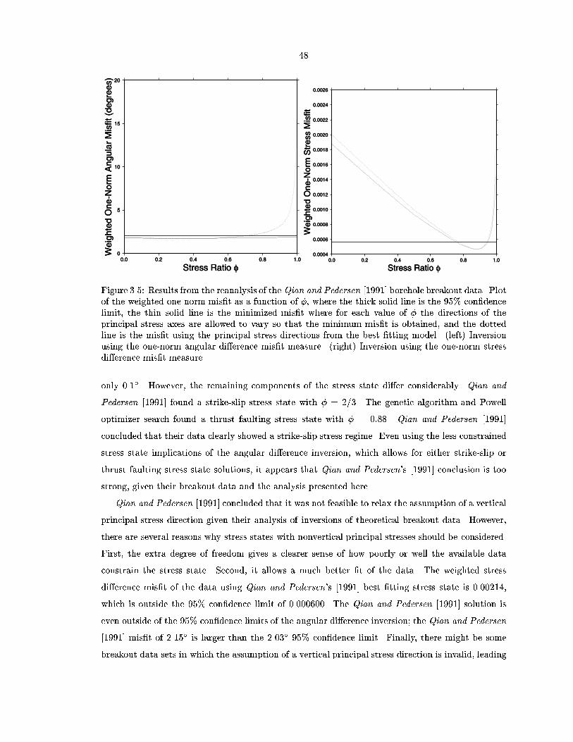
0
5
10
15
20
Wei
ghte
d O
ne-N
orm
Ang
ular
Mis
fit (
degr
ees)
0.0 0.2 0.4 0.6 0.8 1.0
Stress Ratio φ
0
5
10
15
20
Wei
ghte
d O
ne-N
orm
Ang
ular
Mis
fit (
degr
ees)
0.0 0.2 0.4 0.6 0.8 1.0
Stress Ratio φ
0
5
10
15
20
Wei
ghte
d O
ne-N
orm
Ang
ular
Mis
fit (
degr
ees)
0.0 0.2 0.4 0.6 0.8 1.0
Stress Ratio φ
0.0004
0.0006
0.0008
0.0010
0.0012
0.0014
0.0016
0.0018
0.0020
0.0022
0.0024
0.0026
Wei
ghte
d O
ne-N
orm
Str
ess
Mis
fit
0.0 0.2 0.4 0.6 0.8 1.0
Stress Ratio φ
0.0004
0.0006
0.0008
0.0010
0.0012
0.0014
0.0016
0.0018
0.0020
0.0022
0.0024
0.0026
Wei
ghte
d O
ne-N
orm
Str
ess
Mis
fit
0.0 0.2 0.4 0.6 0.8 1.0
Stress Ratio φ
0.0004
0.0006
0.0008
0.0010
0.0012
0.0014
0.0016
0.0018
0.0020
0.0022
0.0024
0.0026
Wei
ghte
d O
ne-N
orm
Str
ess
Mis
fit
0.0 0.2 0.4 0.6 0.8 1.0
Stress Ratio φ
Figure Results from the reanalysis of the Qian and Pedersen borehole breakout data Plotof the weighted onenorm mist as a function of where the thick solid line is the condencelimit the thin solid line is the minimized mist where for each value of the directions of theprincipal stress axes are allowed to vary so that the minimum mist is obtained and the dottedline is the mist using the principal stress directions from the best tting model left Inversionusing the onenorm angular di erence mist measure right Inversion using the onenorm stressdi erence mist measure
only However the remaining components of the stress state di er considerably Qian and
Pedersen found a strikeslip stress state with The genetic algorithm and Powell
optimizer search found a thrust faulting stress state with Qian and Pedersen
concluded that their data clearly showed a strikeslip stress regime Even using the less constrained
stress state implications of the angular di erence inversion which allows for either strikeslip or
thrust faulting stress state solutions it appears that Qian and Pedersens conclusion is too
strong given their breakout data and the analysis presented here
Qian and Pedersen concluded that it was not feasible to relax the assumption of a vertical
principal stress direction given their analysis of inversions of theoretical breakout data However
there are several reasons why stress states with nonvertical principal stresses should be considered
First the extra degree of freedom gives a clearer sense of how poorly or well the available data
constrain the stress state Second it allows a much better t of the data The weighted stress
di erence mist of the data using Qian and Pedersens best tting stress state is
which is outside the condence limit of The Qian and Pedersen solution is
even outside of the condence limits of the angular di erence inversion the Qian and Pedersen
mist of is larger than the condence limit Finally there might be some
breakout data sets in which the assumption of a vertical principal stress direction is invalid leading

to an improper understanding of a regions stress state The cost of this extra degree of freedom is
slight in comparison with the potential gain in understanding of stress states
In conclusion while the stress di erence mist inversion uses a more physically realistic mist
approach to tting borehole breakout data the angular di erence inversion can produce very sim
ilar stress state inversion results The largest di erence between the two mist measure inversion
techniques when applied to the Qian and Pedersen data is the implication regarding the
best tting stress state resulting from the smaller condence limits in the stress di erence in
version Also relaxing the constraint of having a vertical principal stress may allow a much better
determination of the stress state and introduce stress state solutions that t the data much better
Chapter Analysis of the Point Pedernales Data
The borehole breakout inversion technique is applied to wells drilled by the Unocal Company from an
o shore platform in the Point Pedernales oil eld to determine the state of stress in the o shore Santa
Maria Basin California Figure The o shore Santa Maria Basin is an elongated structural
basin parallel to the California coast northwest of Point Arguello McCulloch It lies between
two NNWtrending structural boundaries a zone of eastdipping normal faults including the Santa
Lucia Bank fault on the west side and the Hosgri fault on the east side However it appears to be
stratigraphically continuous with the onshore Santa Maria Basin east of the Hosgri fault and to
have experienced a similar Miocene deformational history Sorlien
The basal Tertiary section in the o shore Santa Maria Basin comprises volcanic rocks of probable
early Miocene age which rest on basement and have been displaced by normal faults McCulloch
This volcanism and a subsequent phase of subsidence Ma documented by use of
backstripping techniques in several wells in the region have been attributed to the capture of the
Monterey microplate by the Pacic plate Sorlien and the beginning of clockwise rotation of the
western Transverse Ranges McCrory et al This development was followed by slow thermal
subsidence from to Ma McCrory et al Since Ma the tectonics of this o shore
region has been locally complicated because of an overall transpressional regime which produced
NESW directed shortening between and Ma and much slower deformation in Quaternary time
eg Clark et al Crouch et al
Unocal provided ve paper logs of four wells from the Point Pedernales eld All four wells
were drilled from the same platform and all of the dipmeter data lies within a km radius of the
platform Table lists the type of tool used to log each hole and some of the properties of the
wells including the logged depth interval the depth interval of processed dipmeter data and the
maximum deviation of the well over the processed interval
The raw dipmeter data was run through a series of steps to analyze it for the ambient tectonic
stress The steps were as follows
Digitize the paper logs and resample them to m intervals
Apply caliper calibration corrections to the caliper arm data for those wells in which the
well log shows a caliper correction
Compare the dipmeters borehole azimuth data with the data from an independent direc
tional survey of the hole singleshot deviation surveys or gyroscopic logs If the two data sets di er
by roughly the magnetic declination E for this location then apply the declination correction

238˚
238˚
239˚
239˚
240˚
240˚
241˚
241˚
242˚
242˚
33˚ 33˚
34˚ 34˚
35˚ 35˚
36˚ 36˚
LA
SB
SLBF
HF
Pacific Ocean
Figure Location star of the Point Pedernales eld in the o shore borderland along with someof the major Quaternary faults in the southern California region LA downtown Los Angeles SBSanta Barbara SLBF Santa Lucia Bank Fault and HF Hosgri Fault
Table Digitized well logs from the Unocal Company of wells drilled o shore from Point Pedernales California in the Santa Maria Basin
Processed TrueLogged Depth Vertical Depth Maximum
Well Name Log Type Interval m Interval m DeviationA Gearhart four logged
electrode processeddipmetersurvey
A Gearhart six logged
electrode processeddipmetersurvey
A Log Schlumberger logged
SHDT processedmonitorlog
A Log Schlumberger logged
dipmeter processedmonitorlog
A Schlumberger logged
formation processedmicroscannerlog
Two separate paper logs were received for well A Logged depth is measured along the wellbore but is greater than the true vertical depth where the borehole is deviated
to the dipmeters borehole azimuth and pad azimuth the XYZ azimuth of the number dipmeter
pad data The declination correction was applied to A and A The data from A and A
agreed with their directional surveys to within and hence were not further corrected
Calculate the borehole elongation direction using the four and sixarm technique de
scribed above Section These data are plotted at every meter in Figure as lower hemisphere
stereographic projections of the borehole elongation Also shown are enlargements of certain regions
of the plot to better show the borehole elongation directions
Select breakouts from the borehole elongation data using the breakout selection criteria
described above Section As an example the calibrated caliper and declinationcorrected
digitized dipmeter data and derived quantities are plotted as a function of log depth with the
selected breakouts from well A in Figure borehole breakouts were identied in the Point
Pedernales caliper arm data Two NS oriented short borehole breakouts from A were manually
removed from the list of breakouts since they were perpendicular to the average EW trend of A
borehole breakouts The remaining breakouts total m in length and are plotted in Figure
No breakouts due to key seats were manually removed from the list of computer selected breakouts
Note that no breakouts were found in the data from well A because of the odd character of the
data from the caliper arms which routinely showed caliper arm diameters quite a bit larger and
smaller than the bit size and caused the data to fail at matching criterion described earlier Since
well A was the only well logged with a sixarm dipmeter the particular technique used to calculate
sixarm borehole elongation angles becomes moot
Figure shows a histogram of the angular di erences between the location of the high and low
sides of the borehole and the breakout angle measured in the plane perpendicular to the borehole
axis for all of the selected breakouts There is roughly a spread of breakout angles about the
high side of the hole These data show the same clustering of breakout angles near the high and low
sides of the hole as Qian and Pedersens data Figure
Invert the selected breakout data for the best tting stress state using the combined GA
and Powell optimization technique described above with both the angular di erence mist measure
m equation and the stress di erence mist measure m equation The results of the
inversions are shown in Tables and
Analogous to the inversion results from the reanalysis of the Qian and Pedersen data the
angular di erence and stress di erence results of the Point Pedernales inversion are very similar and
the stress di erence inversion has much smaller condence limits The condence limits
on the principal stress directions determined by the stress di erence inversion are smaller than the
digits used to plot the orientations of the principal stresses in Figure While the two inversions
found very similar stress states and locations of nodal points compare Tables and Table the
inversion results di er enough from each other that neither the principal stress directions nor the

N
S
EW
15
30
45
60
75
90-1802.3
-604.7
A-7
A-1
A-13
A-16
A-1 A-7
-1802.3
-604.7
A
A-13
A-16
Figure Lower hemisphere stereographic projection plots of the azimuth of borehole elongationat m log depth intervals from the four wells drilled in the Point Pedernales eld top Lowerhemisphere with all the well data plotted bottom Enlargements of the top gure The graduateddepth scale shows the true vertical depth in meters

Pad 1 azimuth
Borehole elongation azimuth
Borehole azimuth
Bitsize
Caliper 1
BreakoutsBreakout
Caliper 2
Borehole deviation
Breakouts
28
30
32
34
36
38
40
42
Cal
iper
Arm
s (c
entim
eter
s)
600 800 1000 1200 1400 1600 1800
Log Depth (meters)
28
30
32
34
36
38
40
42
600 800 1000 1200 1400 1600 180028
30
32
34
36
38
40
42
600 800 1000 1200 1400 1600 180028
30
32
34
36
38
40
42
600 800 1000 1200 1400 1600 1800
0
1
2
3
4
5
6
7
8
Dev
iatio
n (d
egre
es)
600 800 1000 1200 1400 1600 18000
1
2
3
4
5
6
7
8
600 800 1000 1200 1400 1600 1800
0
100
200
300
400
Azi
mut
hs (
degr
ees)
600 800 1000 1200 1400 1600 18000
100
200
300
400
600 800 1000 1200 1400 1600 18000
100
200
300
400
600 800 1000 1200 1400 1600 18000
100
200
300
400
600 800 1000 1200 1400 1600 1800
Figure Plots of the calipercalibrated and declinationcorrected digitized dipmeter data andderived quantities as a function of log depth from well A top Borehole elongation directionsolid line pad azimuth long dashed line and borehole azimuth short dashed line middleBorehole deviation bottom Bit size straight solid line caliper arm solid line and caliperarm dashed line Selected breakout regions are plotted as horizontal bars showing the depthextent of the breakouts
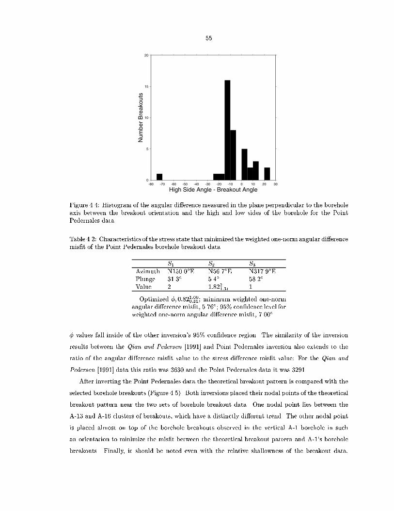
0
5
10
15
20
Num
ber
Bre
akou
ts
-80 -70 -60 -50 -40 -30 -20 -10 0 10 20 30
High Side Angle - Breakout Angle
Figure Histogram of the angular di erence measured in the plane perpendicular to the boreholeaxis between the breakout orientation and the high and low sides of the borehole for the PointPedernales data
Table Characteristics of the stress state that minimized the weighted onenorm angular di erencemist of the Point Pedernales borehole breakout data
S S SAzimuth NE NE NEPlunge
Value
Optimized minimum weighted onenormangular di erence mist condence level forweighted onenorm angular di erence mist
values fall inside of the other inversions condence region The similarity of the inversion
results between the Qian and Pedersen and Point Pedernales inversion also extends to the
ratio of the angular di erence mist value to the stress di erence mist value For the Qian and
Pedersen data this ratio was and the Point Pedernales data it was
After inverting the Point Pedernales data the theoretical breakout pattern is compared with the
selected borehole breakouts Figure Both inversions placed their nodal points of the theoretical
breakout pattern near the two sets of borehole breakout data One nodal point lies between the
A and A clusters of breakouts which have a distinctly di erent trend The other nodal point
is placed almost on top of the borehole breakouts observed in the vertical A borehole in such
an orientation to minimize the mist between the theoretical breakout pattern and As borehole
breakouts Finally it should be noted even with the relative shallowness of the breakout data

Table Characteristics of the stress state that minimized the weighted onenorm stress di erencemist of the Point Pedernales borehole breakout data
S S SAzimuth NE NE NEPlunge
Value
Optimized minimum weighted onenormstress di erence mist condence level forweighted onenorm stress di erence mist
the deepest breakout being km deep the stress state has no vertical principal stress direction
since the nodal points are not symmetric about the origin of the plot unlike the simple stress state
examples shown in Figure The minimum stress S is the closest principal stress direction to
vertical being away from vertical
Because the locations of the two nodal points are reasonably well constrained by the data and
the ratio is directly related to the distance between the two nodal points Figure the ratio
is reasonably well constrained at the condence level Figure Compare this to the Qian
and Pedersen inversion results where the nodal points were not constrained by the borehole
breakout data and hence the ratio was unconstrained for the angular di erence mist
To see if the second nodal points location was only determined by the small scale variation in
As borehole azimuth borehole deviation and breakout angle data an inversion was performed of
a gridded Point Pedernales data set containing only breakouts one of which represented the near
vertical A breakouts The inversion results were almost identical to the results of the nongridded
inversion suggesting that the nongridded inversion did t the larger borehole breakout pattern
while at the same time minimizing the mist between the theoretical breakout pattern and As
breakouts
The small condence limits on the principal stress directions obtained from the stress di er
ence inversion Figure are probably due to the limited number of borehole breakouts identied
at di erent borehole orientations Since the inversion was able to place the two nodal points on top
of both subsets of borehole breakouts and the stress di erence mist for each identied breakout is
small near the nodal points Section the accumulated mist for the Point Pedernales inversion
is very small A slight change in the stress state will move the nodal points further away from the
breakouts and cause the mist to quickly grow much larger than the condence mist hence
leading to the articially small condence limits on the principal stress directions For this
reason and since the principal stress directions and values for the angular di erence and stress
di erence inversions are almost identical the stress di erence inversion results will not be used in
the analysis of the Point Pedernales stress regime

N
S
EW
15.0
30.0
45.0
60.0
75.0
90.0-1265.5
-622.9N
S
EW
15.0
30.0
45.0
60.0
75.0
90.0-1265.5
-622.9
Figure Compiled and processed Point Pedernales borehole breakout data plotted on top of thetheoretical breakout pattern for a best tting stress state generated using the genetic algorithm andPowell optimizer inversion technique Solid circles are nodal points at which the stress anisotropyis zero corresponding to borehole orientations with no preferred breakout direction A Poissonsratio of was used to calculate the breakout pattern The vertical depth scale is in meters leftTheoretical breakout pattern from the onenorm angular di erence mist measure inversion rightTheoretical breakout pattern from the onenorm stress di erence mist measure inversion
The best t orientation of the greatest principal stress direction S is NE plunging
for the angular di erence inversion The condence levels on this S direction would permit
it to lie in the azimuth range from NW to NE Figure If the borehole breakouts
identied in the nearly horizontal wells A and A are not naturally occurring breakouts but
caused by some other mechanism such as tool drag then a simple estimate of SH can be made if
the stress state is assumed to have a vertical principal stress direction In this case only the near
vertical A breakouts remain Using the weighted binning technique Section the average
A borehole breakout azimuth is NE This corresponds to an SH orientation of NE This
orientation of SH falls within the angular di erence condence limits Figure
Other studies have estimated the state of stress in the Santa Maria Basin and the western
Transverse Ranges using geologic earthquake borehole breakout and fracture data Table
Feigl et al used GPS receivers to calculate strain rates and orientations in small triangular
portions of Central and Southern California If the assumption is made that the principal strain axes
are colinear with the principal stress axes then the maximum horizontal principal stress direction
in o shore Santa Maria Basin encompassed by the three GPS stations BLAN Navy Dept Naval
District LOSP Mt Lospe Vandenberg AFB and VNDN VLBI STA RM DET
GSS is oriented NE The results presented by Huang were obtained by performing a

0˚
315˚
270˚
225˚
180˚
135˚
90˚
45˚
1
2
3
1
2
3
1
2
3
0˚
315˚
270˚
225˚
180˚
135˚
90˚
45˚
1
2
3
1
2
3
1
2
3
Figure Results from the analysis of the Point Pedernales borehole breakout data Lower hemisphere stereographic projection plot where the digits and show the optimized orientation ofthe S S and S principal stress axes respectively The weighted onenorm mist condencelimits of the S S and S orientations are plotted as thick solid lines thin solid lines and dottedlines respectively left Inversion using the onenorm angular di erence mist measure The stressstate ratio is held constant at Inner contours are the condence limits right Inversionusing the onenorm stress di erence mist measure is held constant at The condencelimits are smaller than the size of the and digits

0
10
20
30
40
50
60
Wei
ghte
d O
ne-N
orm
Ang
ular
Mis
fit (
degr
ees)
0.0 0.2 0.4 0.6 0.8 1.0
Stress Ratio φ
0
10
20
30
40
50
60
Wei
ghte
d O
ne-N
orm
Ang
ular
Mis
fit (
degr
ees)
0.0 0.2 0.4 0.6 0.8 1.0
Stress Ratio φ
0
10
20
30
40
50
60
Wei
ghte
d O
ne-N
orm
Ang
ular
Mis
fit (
degr
ees)
0.0 0.2 0.4 0.6 0.8 1.0
Stress Ratio φ
0.0
0.1
0.2
0.3
0.4
0.5
Wei
ghte
d O
ne-N
orm
Str
ess
Mis
fit
0.0 0.2 0.4 0.6 0.8 1.0
Stress Ratio φ
0.0
0.1
0.2
0.3
0.4
0.5
Wei
ghte
d O
ne-N
orm
Str
ess
Mis
fit
0.0 0.2 0.4 0.6 0.8 1.0
Stress Ratio φ
0.0
0.1
0.2
0.3
0.4
0.5
Wei
ghte
d O
ne-N
orm
Str
ess
Mis
fit
0.0 0.2 0.4 0.6 0.8 1.0
Stress Ratio φ
Figure Results from the analysis of the Point Pedernales borehole breakout data Plot of theweighted onenorm mist as a function of where the thick solid line is the condence limitthe thin solid line is the minimized mist where for each value of the directions of the principalstress axes are allowed to vary so that the minimum mist is obtained and the dotted line is themist using the principal stress directions from the best tting model left Inversion using theonenorm angular di erence mist measure right Inversion using the onenorm stress di erencemist measure
stress state inversion of M earthquakes that occurred in the western Transverse Ranges
the Santa Barbara Channel and the Santa Maria Basin Region from to Huang
reports S oriented NE inclined away from the horizontal The stress state results presented
by Mount and Suppe are calculated using the average breakout azimuth observed in the O
O and O wells in the Santa Maria Basin presented in their paper Assuming that the breakout
orientation is perpendicular to the SH azimuth then SH is oriented NE Varga and Hickman
studied naturally tensile occurring fractures observed in drill cores obtained from well A in
the Point Pedernales eld and observed an average fracture azimuth of NE suggesting that the
maximum horizontal stress was oriented in the same direction when the fractures were created The
di erence in the fracture azimuth and the SH azimuth determined from the borehole breakouts in
the same hole di er suggesting a change in the stress state since the time when the fractures formed
Clark et al
While the stress state results for the Santa Maria Basin and western Transverse Ranges show a
large amount of variation Figure the stress inversion results using the breakouts identied in
both the vertical and horizontal boreholes is completely di erent than the other stress state results
This suggests that either the stress state in the Point Pedernales is eld very di erent than that
of surrounding regions or that the borehole breakout data are suspect Since the SH azimuth

Table Stress state results from studies performed in the Santa Maria basin and the westernTransverse Ranges
Study Measurement Type S or SH Azimuth InclinationThis study Borehole breakouts S NE
This study Borehole breakouts SH NE
Huang Earthquake focal mechanisms S NE
Mount and Suppe Borehole breakouts SH NE
Varga and Hickman Fractures in boreholes SH NE
A Global Positioning System GPS survey of the o shore Point Pedernales area by Feigl et al determined a principle strain shortening azimuth of NE
calculated using the vertical A borehole is fairly consistent with the other stress state studies
it appears that the stress state results using the complete breakout data set are controlled by the
poor borehole orientation coverage and the fact that the inversion process places the breakout nodal
points near the data For this reason the general threedimensional stress results are inconclusive
and require better data coverage to gain an understanding of the complete stress state in the o shore
Santa Maria Basin using this technique More complete coverage of the borehole orientation space
represented by the plot in Figure would also allow a better estimation of the overall variability
of the measurements and show whether the inferred positions of the nodal points are likely to be
correct on a more regional scale

A
B
B
C
C
D
E
E
F
F
0˚
270˚
180˚
90˚
0˚
270˚
180˚
90˚
Figure Lower hemisphere stereographic projection plot of S or SH orientations from studiesperformed in the Santa Maria basin and the western Transverse Ranges The contours are the same and angular di erence condence limits plotted in Figure The letters AF refer tothe stress state results generated by A all the Point Pedernales breakouts identied in this studyB Point Pedernales breakouts identied in the vertical A well C Feigl et al D Huang E Mount and Suppe F Varga and Hickman

Chapter The Stress State and Its Depth
Dependence in Cook Inlet Alaska
Abstract
The stress state and its depth dependence in Cook Inlet Alaska were determined using breakouts
identied in deviated boreholes drilled from o shore oil platforms in Cook Inlet Twentyone separate
boreholes reaching deviations of and m true vertical depth were examined from ve
o shore oil platforms that produce oil from narrow NNEtrending anticlines Granite Point Anna
and Bruce platforms in the Granite Point eld and Baker and Dillon platforms in the Middle
Ground Shoals eld The breakouts were calculated from analog and digital dipmeter and formation
microscanner FMS data
A total of usable breakouts totaling m in length were identied of these breakouts
totaling m in length had their breakout orientations at least away from the low and high
side of the borehole ie nonradial Stress state inversions of di erent subsets of the borehole
breakout data were performed Inversion of breakouts identied in the top and middle marker beds
of three marker beds analyzed in wells drilled from the Baker platform identied nearly degenerate
thrust faulting stress states with the maximum principal stress axis S oriented horizontallyWNW
ESE perpendicular to the NNEtrending anticlinal structures The stress state from the deepest
marker is also a nearly degenerate thrust faulting stress state with S oriented NNWSSE aligned
with the regional direction of relative plate motion between the North American and Pacic plates
In between the shallow and deep stress state is an observed normal faulting stress state with S
oriented subhorizontally ENEWSW This clockwise rotation of the stress tensor as a function of
depth suggests that the stress eld changes from a shallow stress state responsible for the local NNE
trending structures and a deeper one from the North American and Pacic plates collision zone The
observed normal faulting stress state between the two thrust faulting stress states is anomalous and
may represent some sort of transition from the shallow to the deep stress state Stress state proles
in m true vertical depth TVD intervals show consistently oriented thrust faulting NNWSSE
trending S azimuths The thrust faulting S principal stress direction is consistently within
of vertical suggesting that the stress tensor does not signicantly rotate away from the surface
conditions that require a purely vertical stress tensor However the deviation of the S
axes implies that the assumption of a purely vertical principal stress direction is not valid The

180˚
180˚
190˚
190˚
200˚
200˚
210˚210˚
220˚
220˚
230˚
240˚
60˚60˚
65˚65˚
70˚ 70˚
180˚
180˚
190˚
190˚
200˚
200˚
210˚210˚
220˚
220˚
230˚
240˚
60˚60˚
65˚65˚
70˚ 70˚
208˚
208˚
209˚
209˚
210˚
210˚
211˚
211˚
61˚ 61˚
208˚
208˚
209˚
209˚
210˚
210˚
211˚
211˚
61˚ 61˚
208˚
208˚
209˚
209˚
210˚
210˚
211˚
211˚
61˚ 61˚
208˚
208˚
209˚
209˚
210˚
210˚
211˚
211˚
61˚ 61˚
208˚
208˚
209˚
209˚
210˚
210˚
211˚
211˚
61˚ 61˚
208˚
208˚
209˚
209˚
210˚
210˚
211˚
211˚
61˚ 61˚
208˚
208˚
209˚
209˚
210˚
210˚
211˚
211˚
61˚ 61˚GP
MGS
Anchorage
Bor
der
Ran
ges
Faul
tE
agle
Riv
er F
ault
Castle M
ountain Fault
Lake Clark Fault
Brui
n Ba
y Fa
ult
208˚
208˚
209˚
209˚
210˚
210˚
211˚
211˚
61˚ 61˚
208˚
208˚
209˚
209˚
210˚
210˚
211˚
211˚
61˚ 61˚
Figure left Stereographic projection map of Alaska The boxed area in this plot is shown inthe right plot right Mercator projection of Cook Inlet Alaska plotting major structural faultsthick lines minor faults thin lines the oil elds examined in this study thin ellipses and theo shore oil platforms where deviated boreholes were drilled from triangles The northern oil eldis Granite Point GP and the southern oil eld is Middle Ground Shoals MGS From northto south the platforms are Granite Point Bruce Granite Point Anna Granite Point Granite PointMiddle Ground Shoals Baker and Middle Ground Shoals Dillon
nearly degenerate thrust faulting stress states inverted from the Granite Point and the km
distant Baker platform breakouts are nearly identical implying that the technique of using deviated
borehole breakouts to invert for the regional stress is valid The orientations of the maximum
horizontal stress determined from the Cook Inlet borehole breakouts are consistent with other stress
indicators in southcentral Alaska and consistent with the direction of relative plate motion between
the North American Plate and the Pacic plate The S axis for the Cook Inlet eld trends NE
plunging but does not appear representative of the stress eld for each subset of breakouts The
Granite Point S axis trends NW plunging the Baker platform S axis trends N
W
plunging and the Dillon platform S axis trends NW plunging The more westerly
Dillon platform S orientation of the may be related to the local NNEtrending anticlinal structures
in the Cook Inlet Basin
Introduction
The stress state inversion technique developed in previous chapters determines the orientation and
relative magnitudes of the principal stress orientations from a set of borehole breakouts identied in
deviated boreholes Previous applications of this technique used borehole breakout data sets with
limited depth and borehole deviation and borehole azimuth coverage Here the technique is applied

to a large breakout data set covering a km region obtained from wells drilled into the Middle
Ground Shoals and Granite Point oil elds in Cook Inlet Alaska where borehole breakouts were
identied between and m true vertical depth The large quantity of data allows stress
state inversions of smaller subdivisions of the data and an examination of stress state changes as
a function of depth The principal stress directions and the stress state ratio may change as a
function of depth for many reasons the stress ratio can change as the overburden pressure
increases with depth Chapter the stress state may change as the borehole enters into
di erent areas of the local geologic structure and di erent geologic formations have di erent
material properties
This chapter begins by discussing the geology and stratigraphy of the Cook Inlet Basin then
examines the data processing and analysis issues that emerged and were resolved in this study The
data from each borehole are individually examined and analyzed Finally data are then inverted
and the results are discussed
Geology and Stratigraphy of the Cook Inlet Basin
Cook Inlet is a very large estuary in south central Alaska with Anchorage lying at its northeastern
end It lies within the Cook Inlet Basin which is a km long km wide NNESSW striking
forearc basin in the Pacic and North American plate subduction margin Figures and The
tectonic framework of southern Alaska and the Cook Inlet Basin is dominated by the convergence
between the subducting Pacic Plate and the overriding North American plate The region is
tectonically complex given that it lies between the purely convergent margin along the Aleutian
trench to the west and the transform plate boundary to the east expressed by the Fairweather and
Queen Charlotte faults
The Cook Inlet Basin is about the same size as the San Joaquin Basin and shares many of the
same structural settings Boss et al It is bounded on the north and west by the Bruin Bay
and Castle Mountain faults and the AlaskaAleutian Range Figure On the south and east it
is bounded by the Border Ranges fault and by the Kenai Mountains The Border Ranges fault is a
km long suture that can be traced from Baranof Island in the Alaskan panhandle to Kodiak
Island It separates a forearc basin sequence on the Peninsular terrane on the northern side of the
fault from rocks inferred to have been deposited in a subduction accretionary complex Chugach
terrane Figure and shares many analogies with Californias Coast Range fault system Boss
et al Little and Naeser Plafker et al Both terranes are exotic to Alaska and the
Chugach terrane is the more newly accreted terrane Schmoll et al In the Cook Inlet area the
Border Ranges fault separates the Chugach terrane on the south from preLate Cretaceous sequence
and correlative rocks of the AlaskaAleutian Range batholith Magoon The Border Ranges

fault has history of Early Jurassic through Late Cretaceous subduction In places it is o set and
modied by younger strikeslip and normal faults Little and Naeser Plafker et al
Recent seismicity may be associated with the Border Ranges fault however uncertainties in the
epicentral locations cannot denitely relate earthquakes with the Border Ranges fault Ratchkovsky
et al
The Castle Mountain fault is the northern boundary to the Cook Inlet Basin The fault displays
Holocene obliqueslip o sets and has been historically active In a buried km segment of the
Castle Mountain fault broke to generate the mb Sutton earthquake which involved rightlateral
slip Page et al The Castle Mountain fault is one of at least three fault systems that absorb
the relative plate motion between the subducting Pacic Plate and the deforming North American
plate
The western boundary of the Cook Inlet Basin is the Bruin Bay fault a major northeasttrending
fault that has been mapped from near Mt Spurr to Becharof Lake for km and may extend an
additional km to the southwest Miller and Richter It along with the Lake Clark fault
is a probable southwestern extension of the Castle Mountain fault Detterman et al The
Bruin Bay fault is a highangle reverse fault and displays evidence of up to km of stratigraphic
throw Nokleberg et al There is no evidence of Holocene displacement on either the Bruin
Bay or the Lake Clark faults This fault zone is at least of Middle Jurassic age but some of its small
highangle faults in the northwest have Miocene movement No signicant lateral displacement is
associated with this fault Boss et al
In the Cook Inlet area most of the oil and gas is produced from rocks in the Kenai Group which
range in age from the Upper Oligocene through Upper Pliocene and unconformably overlie source
rocks of Mesozoic age Magoon Wahrhaftig et al The Kenai Group is composed from
older to younger of the Hemlock Conglomerate the Tyonek Formation the Beluga Formation and
the Sterling Formation The Oligocene Hemlock Conglomerate which contains of the oil in
Cook Inlet consists of conglomerate and conglomeratic sandstone containing quartz and chert and
pebbles of metamorphic volcanic and plutonic rocks Magoon Wahrhaftig et al It
also contains a few thin coal seams Boss et al The Tyonek Formation consisting of as
much as m of sandstone conglomeratic sandstones shale conglomeratic shales and coal beds
deposited in a braidedstream environment is of Lower Oligocene through middle Miocene age The
Tyonek Formation contains the bulk of the coal resources in Cook Inlet The Beluga Formation is of
Upper and Middle Miocene age and it along with the Sterling Formation are the major producers
of methane gas in Cook Inlet The whole formation is of continental origin with a large variation of
lithologies This formation consists of oodplain shales with minor interbedded coal seams and thin
channel sandstones Boss et al The Sterling Formation is of latest Miocene and Pliocene age
and consists of massive sandstone conglomeratic sandstone and interbedded claystone and some

yyyyyyyyyyyyyyyyyyyyyyyyyyyyyy
yyyyyyyyyyyyyyyyyyyyyyyyyyyyyyyyyyyyyyyyyyyyyyyyy
yyyyyyyyyyyyyyyyyyyyyyyyyyyyyyyyyyyyyyyyyyyyyyyyyyyyyyyyyyyyyyyyyyyyyyyy
yyyyyyyyyyyyyyyyyyyyyyyyyyyyyyyyyyyyyyyyyyyyyyyyyyyyyyyy
yyyyyyyyyyyyyyyyyyyyyyyy
yyyyyyyyyyyyyyyyyyyyyyyyyyyyyyyyyyyyyyyyyyyyyyyyyyyyyyyyyyyyyyyyyyyyyyyyyyyyyyyyyyyyyyyyyyyyyyyyyyyyyyyyyyyyyyyyyyyyyyyyyyyyyyyyyyyyyyyyyyyyyyyyyyyyyyyyyyyyyyyyyyyyyyyyyyyyyyyyyyyyyyyyyyyyyyyyyyyyyyyyyyyyyyyyyyyyyyyyyyyyyyyyyyyyyyyyyyyyyyyyyyyyyyyyyyyyyyyyyyyyyyyyyyyyyyyyyyyyyyyyyyyyyyyyyyyyyyyyyyyyyyyyyyyyyyyyyyyyyyyyyyyyyyyyyyyyyyyyyyyyyyyyy
yyyyyyyyyyyy
yyyyyyyyyyyyyyyyyyyyyyyyyyyyyyyyyyyyyyyyyyyyyyyyyyyyyyyyyyyyyyyyyyyyyyyyyyyyyyyyyyyyyyyyyyyyyyyyyyyyyyyyyyyyyyyyyyyyyyyyyyyyyyyyyyyyyyyyyyyyyyyyyyyyyyyyyyyyyyyyyyyyyyyyyyyyyyyyyyyyyyyyyyyyyyyyyyyyyyyyyyyyyyyyyyyyyyyyyyyyyyyyyyyyyyyyyyyyyyyyyyyyyyy
yyyyyyyyyyyyyyyy
yyyyyyyyyyyyyyyyyyyyyyyyyyyyyyyyyyy
yyyyyyyyyyyyyyyyyyyyyyyyyyyyyy
yyyyyy
yyyyyy
yyyyyy
yyyyy
yyyyyyyyyyyyyyy
yyyy
yyyyyyyyyyyyyyyyyyyyyy
yyyyyyyyy
yy
yyyyyy
yyyyyyyyyyyy
yy
yy
yyyy
yyy
yy
yyyy
yyyy
yyy
y
yyyyyyyy
yyyyyy
yyyyyy
yyyyyyyy
yyyyyyyyyyyy
yyyyyyyyyyyy
yyyy
yyyy
Coo
kIn
let
Anchorage
Valdez
Con
tact
Faul
t
Bruin
Bay
Fa
ult
Bor
der
Ran
ges
Faul
t
Castle Mtn. Fault
Lake Clar
kFau
lt
152o
146o
60o
62o
146o
152o
60o
62o
QsKJ
TKs KJch
Tspw
TMi
TMi TMiKJ
MPwp
TKs
TKs
Tspw
KJch
MPwp
Qs
TKs
TKs
TKs
Cretaceous and Tertiary Sedimentary Rocksincluding Cook Inlet forearc deposits
yyyyyy
TKs
Mesozoic and Paleozoic Rocks of the Peninsular and Wrangellia Terranes
yyMPwp
Quaternary Sediments and Volcanic RocksQs
Tertiary Sedimentary Rocks of the Prince William TerraneyyTspw
Cretaceous and Jurassic Sedimentary Rocks of the Chugach TerraneyyKJch
Mesozoic and Tertiary Igneous Rocksprimarily intrusives
yyyyyyyyyyyyyyyyyyyyyyyyyyyyyyyyyyy
TMi
Cretaceous and Jurassic Sedimentary and Metasedimentary Rocks
yyyyKJ
GP
MGS
0 50 150 km
GP Granite Point Oil FieldMGS Middle Ground Shoals Oil Field
Figure Geologic and terrane map of Cook Inlet Alaska modied from Bunds et al TheGranite Point and Middle Ground Shoals oil elds are shown as small empty ellipses

thin coal and tu beds It reaches a maximum thickness of m Wahrhaftig et al and
contains most of the gas reservoirs in the Cook Inlet Basin Magoon
The typical Cook Inlet oil elds lie in narrow NNESSW trending anticlines whose major growth
occurred very late in the Tertiarylate Pliocene andor early Pleistocene time Boss et al
The anticlines are overlain by Pleistocene to recent undeformed atlying sediments suggesting
that they are no longer active The Middle Ground Shoal oil eld lies in the center of the Cook
Inlet basin roughly km by air southwest of Anchorage Alaska beneath an average of m of
water The oilproducing section of this eld is a narrow anticline which is up to km long and
km wide striking NE The east ank dips from to east The southern end plunges
gently to the southsouthwest at about The western ank of the anticline dips between and
and may contain some eastdipping reverse faults one of which may transect the northern end
of the structure The Middle Ground Shoal eld produces oil from a gross interval of roughly m
in the lower Tyonek Formation between and m depth Boss et al
The Granite Point oil eld lies approximately km NNE of the Middle Ground Shoal oil eld
and km southwest of Anchorage Like the Middle Ground Shoals eld the oil producing interval
is a km long and km wide northnortheast trending slightly asymmetrical anticline where
the east ank dips E and the west ank dips W Laughbaum et al
Data Description and Processing
Oshore Oil Platforms and Summary of Raw Data
The Unocal Company provided dipmeter data from ve di erent o shore oil platforms located in
two oil elds platforms Granite Point Anna and Bruce in the Granite Point eld and platforms
Baker and Dillon in the Middle Ground Shoals eld Figure The ve oil platforms are fairly
close to each other using the Baker platform as a reference Dillon is km away at SW
Anna is km away at NE Bruce is km away at NE and Granite Point is km
away at NE
Throughout this chapter specic wells and well log data sets are referred to by abbreviations
wells drilled in the Granite Point eld are abbreviated Gp eg Gprd wells drilled in the
Middle Ground Shoals eld from the Baker platform are abbreviated Mgs eg Mgsrd and the
wells drilled in the Middle Ground Shoals eld from the Dillon platform are abbreviated Smgs S
for south eg Smgs All wells drilled in the Granite Point eld from either the Granite Point
Anna or Bruce platforms are referred to as Gp A name followed by the characters rd refer to
a redrilled well eg Gprd See Table for a summary of the wells analyzed and some of their
properties
Figures and show paths of the wells in map view from the Granite Point platforms
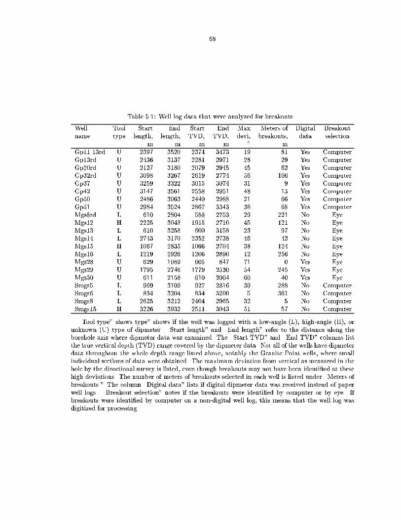
Table Well log data that were analyzed for breakouts
Well Tool Start End Start End Max Meters of Digital Breakoutname type length length TVD TVD devi breakouts data selection
m m m m mGprd U Yes ComputerGprd U Yes ComputerGprd U Yes ComputerGprd U Yes ComputerGp U Yes ComputerGp U Yes ComputerGp U Yes ComputerGp U Yes ComputerMgsrd L No EyeMgs H No EyeMgs L No EyeMgs L No EyeMgs H No EyeMgs L No EyeMgs U Yes EyeMgs U Yes EyeMgs U Yes EyeSmgs L No ComputerSmgs L No ComputerSmgs L No ComputerSmgs H No Computer
Tool type shows type shows if the well was logged with a lowangle L highangle H orunknown U type of dipmeter Start length and End length refer to the distance along theborehole axis where dipmeter data was examined The Start TVD and End TVD columns listthe true vertical depth TVD range covered by the dipmeter data Not all of the wells have dipmeterdata throughout the whole depth range listed above notably the Granite Point wells where smallindividual sections of data were obtained The maximum deviation from vertical as measured in thehole by the directional survey is listed even though breakouts may not have been identied at thesehigh deviations The number of meters of breakouts selected in each well is listed under Meters ofbreakouts The column Digital data lists if digital dipmeter data was received instead of paperwell logs Breakout selection notes if the breakouts were identied by computer or by eye Ifbreakouts were identied by computer on a nondigital well log this means that the well log wasdigitized for processing

A
14
16
18
20
Y (
km)
14 16 18
X (km)
B
14
16
18
20
Y (
km)
14 16 18
X (km)
G14
16
18
20
Y (
km)
14 16 18
X (km)
14
16
18
20
Y (
km)
14 16 18
X (km)
Figure Map view of the paths of the wells from the Granite Point G Anna A and BruceB platforms Distances are in meters away from top of the Middle Ground Shoals number redrillborehole
the Baker platform and the Dillon platform respectively All of the platforms show good spatial
distributions of boreholes drilled into di erent regions of the anticlines and a good coverage of the
borehole azimuth borehole deviation space
Well Log Processing
The Baker and Dillon platform dipmeter data are all paper logs except for Mgs Mgs and
Mgs which are digital The Granite Point dipmeter data are also digital Given the large amount
of paper and digital data from di erent welllogging tools Table a few di erent processing
techniques were used to integrate the data together into a consistent whole
All wells were logged with Schlumberger dipmeters The bit size information was not included in
some of the digital dipmeter logs In these cases the bit size was estimated by examining the caliper
arm data and comparing it to one of the common bit sizes that best matched the caliper arm data
cm inches cm inches or cm inches This technique worked
for most of the digital data except for Mgs and Gp Mgs has widely varying caliper arm data
ranging from cm inches to the maximum caliper arm diameter of cm inches
Mgss bit size was cm inches in the upper portion of the hole and decreased to cm
inches in the remaining part of the hole Unocal personal communication Neither of these
bit sizes agree with the caliper arm data Figure B

M
-2
0
2
Y (
km)
-2 0 2
X (km)
-2
0
2
Y (
km)
-2 0 2
X (km)
Figure Map view of the paths of the wells from the Baker platform M in the Middle GroundShoals eld Distances are in meters away from the top of the Middle Ground Shoals number redrill borehole
Some of the paper well logs were digitized for computerized borehole breakout selection and other
paper logs were examined by eye for breakouts All of the paper Baker platform wells were examined
by eye and all of the Dillon platform wells were digitized Sections of the Dillon paper logs were
digitized by a company which specializes in digitizing paper logs and the remaining sections were
digitized at Caltech One complication of the paper well logs is a nonlinear caliper arm scale in
which the spatial location of a data point on the paper log is not a linear function of the caliper arm
diameter This nonlinear caliper arm scale needs to be taken into account when the caliper arm data
are digitized In examining the digitized caliper arm data obtained from the digitizing company it
appears that the nonlinearity was not properly corrected Because of the errors inherent in digitizing
paper well logs I only applied a simple linear o set to the caliper arm data if the digitized data
were much di erent than the caliper arm data plotted on paper
A major complication in the uncorrected dipmeter data is the issue of magnetic declination It is
unclear whether various dipmeter azimuthal measurements such as the borehole and pad azimuths
were measured with respect to magnetic or geographic north Fortunately gyroscopic directional
survey logs which measure the borehole azimuth and deviation as a function of well depth with
respect to geographic north were obtained from Unocal The directional survey information was
used in place of the dipmeter azimuthal measurements In some cases the di erence is on the order
of several degrees but in other cases the azimuthal correction amounts to roughly

D
-12
-10
Y (
km)
-4 -2
X (km)
-12
-10
Y (
km)
-4 -2
X (km)
Figure Map view of the paths of the wells from the Dillon D platform in the Middle GroundShoals eld Distances are in meters away from the top of the Middle Ground Shoals number redrill borehole
Replacing dipmeter azimuth measurements with directional survey data has some advantages
and disadvantages The primary advantage is the consistency in the processing technique and using
a known quantity for the borehole azimuth and deviation data There are two potentially serious
problems One problem occurs when the log depths measured by the two tools are o set from each
other Tools stuck in the hole and cable stretch could lead to a depth di erence between the two
data sets However borehole azimuth and deviation curves do not vary quickly over a m interval
so this issue while important will not be addressed in this thesis The second problem lies with the
di erences between low and highangle dipmeters Lowangle dipmeters are typically used in holes
with deviations less than They measure the pad azimuth and the relative bearing but they
do not measure the borehole azimuth since at low deviations the borehole azimuth can uctuate
widely Highangle dipmeters are used in holes with deviations higher than and measure the
relative bearing and the borehole azimuth Highangle dipmeters do not measure pad azimuths
since at high borehole deviations the map projection of the line drawn from the center of the
dipmeter to the end of pad approaches a constant azimuth regardless of the orientation of pad
If pad azimuths were measured then pad azimuths lying away from the borehole azimuth
would preferentially be measured Given the di erent orientation information measured by the low
and highangle tools di erent techniques are required for integrating the data into a collective whole
These di erences could lead to systematic inconsistencies between data from high and lowangle

tools
It was only possible to positively determine if a low or highangle dipmeter was used to log the
borehole in cases when paper well logs were received In over half of the boreholes Table digital
dipmeter was received and it was presumed that a lowangle dipmeter was used to log the borehole
if digital pad azimuth data were one of the measurements obtained from the well log If borehole
azimuth data were received instead then the dipmeter was presumed to be a highangle dipmeter
Regardless of the style of dipmeter used to log a borehole the data processing calculations properly
transformed the raw dipmeter data into a set of borehole azimuth borehole deviation and IJK
elongation angle as a function of depth along the borehole axis
The directional survey data were also used to calculate the location of the borehole through the
earth as a function of well depth These positional data consisting of the east north and vertical
distance in meters away from the drilling platform were then merged with the breakout data to
obtain the horizontal and vertical location of the breakouts While the same problem of merging the
dipmeter data with directional survey data can lead to a mismatch between the real and calculated
location of the breakout these errors are not considered here since the inversion technique does
not depend upon the breakout location These errors are considered when the breakout location is
compared to the location of known geological structures
Several other processing steps were done while processing the dipmeter and directional survey
data These steps included converting from English to metric units and calibrating the caliper arm
data if the well log showed a calibration measurement
Borehole Breakout Selection
A modied version of the borehole selection criteria described in section was used to identify
more borehole breakouts than would be normally identied Instead of limiting the standard devia
tion of the IJK breakout angle in a breakout to breakouts with IJK breakout angle standard
deviations of were allowed The minimum ellipticity of the breakout was also lowered from
to On the other hand the maximum allowed caliper arm standard deviation was lowered from
cm inch to cm inch
Selection of Borehole Breakout Data Subsets
To study depth dependent and material dependent aspects of the stress state the complete set of
Cook Inlet borehole breakout data was subdivided into various subsets and separately inverted for
the stress state A list of the number of breakouts and the length of breakouts for a particular subset
of breakouts is shown in Table
Material property di erences between adjacent beds or formations can rotate the stress tensor

Bruno and Winterstein To study this e ect in the Cook Inlet data set marker les that
Unocal supplied were used to subdivide the breakouts into di erent The marker les list the well
log depth of horizons of markers horizons of oil pools and the well log depth of faults which the well
may cross The oilproducing interval was separated into seven pools designated A through G
by the State of Alaska Oil and Gas Committee After identifying breakouts in all of the Cook Inlet
wells those markers that contained a large number of breakouts at di erent borehole orientations
were selected and breakouts in those markers were independently analyzed To get larger spatial and
borehole orientation coverage of the breakouts from a set of markers the marker les were examined
to see if the breakouts from two or more markers could be combined Only the G and G markers
from the Baker platform were always adjacent to each other in the marker les and were never
separated by a fault or any other markers In the Granite Point oil eld the TXSS marker was
chosen since this particular Granite Point marker had the most identied breakouts identied
breakouts totaling m in length The Dillon platform wells had breakouts totaling m in
length in the TE marker Enough breakouts were identied in the Baker platform wells such that
several di erent markers could be independently analyzed The chosen markers were BSS with
breakouts totaling m in length D with breakouts totaling m in length and the
combined markers G and G which have breakouts totaling m in length
While the marker data has proven to be very useful no description of the material and elastic
properties of the markers were ever received from Unocal to make this analysis complete The
information would have been helpful since one of the many factors that can cause the rotation of the
stress tensor across the contact between two beds or formations is the contrast between the elastic
properties Bruno and Winterstein
In addition to analyzing the breakouts occurring in particular markers identied breakouts
were also separated into several di erent subsets and analyzed The rst division separated those
breakouts with their IJK breakout angle more than from either the high or low side of the hole
from the remaining breakouts The latter group includes those breakouts that could be caused by
tool drag The former group of breakouts are termed nonradial since the orientation of a breakouts
aligned with the high and low sides of the borehole when plotted on a lower hemisphere stereographic
projection trend radially toward the center of the plot Figure The second separation grouped
breakouts into m true vertical depth intervals to study the depth dependent e ects on the stress
state
Individual Discussion of Wells
Each of the well logs and their identied breakouts were individually analyzed The analysis
included understanding inconsistently oriented breakouts simple stress state analyses for those wells
with a large number of breakouts and evaluation of other problems that needed to be xed with

Table Statistics of various selected subsets of breakouts
Field or Number of Total length ofPlatform Selection breakouts breakouts mAll All All Nonradial All Nonradial between m TVD All Nonradial between m TVD All Nonradial between m TVD All Nonradial between m TVD All Nonradial between m TVD Gp All Gp Nonradial Gp Nonradial between m TVD Gp Nonradial between m TVD Baker All Baker Nonradial Baker Marker BSS Baker Nonradial marker BSS Baker Marker D Baker Nonradial marker D Baker Markers G and G Baker Nonradial markers G and G Baker Nonradial between m TVD Baker Nonradial between m TVD Baker Nonradial between m TVD Baker Nonradial between m TVD Baker Nonradial between m TVD Dillon All Dillon All excluding Smgs Dillon Nonradial Dillon Nonradial excluding Smgs Dillon Marker TE Dillon Nonradial marker TE Dillon Nonradial between m TVD Dillon Nonradial between m TVD Dillon Nonradial between m TVD
Gp refers to those breakouts identied in the Granite Point eld from any of the three oilplatforms The sets of breakouts do not include breakouts from Granite Point or South MiddleGround Shoals since the breakouts from these wells had no consistent breakout orientations andan indepth analysis of the dipmeter logs did not lead to an interpretation of the breakout datawith more consistent orientations Stress state inversions were done on all of these selected breakoutsubsets except those containing fewer than breakouts

the data This analysis is included in Appendix B The major conclusion of this work is that the
breakouts identied in Gp and Smgs are highly inconsistently oriented and a detailed analysis of
these breakouts was unable to determine which of these breakouts could be used in a stress inversion
As such the breakouts from these two wells are not used in any of the following stress inversions
Inversion of Borehole Breakouts
The inversion process described in Chapter was used to invert various groups of borehole breakouts
for the best tting stress tensor The breakouts from Granite Point and South Middle Ground
Shoals were not included in any of the inversions since the breakouts from these wells had no
consistent breakout orientations and an indepth analysis of the dipmeter logs did not lead to an
interpretation of the breakout data with more consistent orientations Removing the breakout data
from these two wells reduced the minimum weighted onenorm mists of the inversion results by
to The inversion results also show much better constrained principal stress directions
A total of breakouts summing to m in length were available for various inversions
Figures show the stress inversion results for di erent subsets of borehole breakouts
Table Each subset was inverted using the angular di erence and stress di erence mist
measure The subsets are all breakouts Figures and all nonradial breakouts Figures
and all nonradial breakouts between and m TVD Figures and all nonradial
breakouts between and m TVD Figures and all nonradial breakouts between
and m TVD Figures and all nonradial breakouts between and m
TVD Figures and all nonradial breakouts between and m TVD Figures
and all Granite Point breakouts Figures and all nonradial Granite Point breakouts
Figures and nonradial breakouts between and m TVD in the Granite Point
eld Figures and and nonradial breakouts between and m TVD in the Granite
Point eld Figures and Inversions of sets of breakouts in wells drilled from the Baker
platform in the Middle Ground Shoals eld are all breakouts Figures and all nonradial
breakouts Figures and all breakouts and all nonradial breakouts occurring in the BSS
marker Figures all breakouts and all nonradial breakouts occurring in the D marker
Figures all breakout and all nonradial breakouts occurring in the G and G markers
Figures nonradial breakouts between and m TVD Figures and
nonradial breakouts between and m TVD Figures and nonradial breakouts
between and m TVD Figures and and nonradial breakouts between
and m TVD Figures and Breakouts in wells drilled from the Dillon platform in
the Middle Ground Shoals eld were analyzed in the following groups all breakouts Figures
and all nonradial breakouts Figures and all breakouts excluding those from Smgs
Figures and all nonradial breakouts excluding those from Smgs Figures and
all breakouts and all nonradial breakouts occurring in the TE marker Figures and
nonradial breakouts between and m TVD Figures and nonradial breakouts
between and m TVD Figures and and nonradial breakouts between
and m TVD Figures and Subsets of data containing less than ve breakouts were
not inverted since the inversion process needs ve breakouts to constrain the three stress tensor
Euler angles and the stress state value
Each gure shows a large amount of information for each individual inversion The upper left
panel shows the number of breakouts and the total length of breakouts used in the inversion the
optimized value of the condence limits on and the minimum and weighted onenorm
mist values for this data set Also shown are the azimuth deviation and stress state magnitudes
for the S S and S principal stresses The upper right plot is a lower hemisphere stereographic
projection plot of breakouts used for the inversion Each breakout plots as a single line with constant
length The width of the line is proportional to the length of the breakout and inversely proportional
to the IJK breakout angle variance over the breakout length Breakouts from shallow depths plot at
dark shades of gray and breakouts from greater depths plot at lighter shades of gray Lines beneath
the breakouts are the predicted orientations of breakouts for the best tting stress state from the
inversion The lower left panel plots the condence limits on the orientation of the principal
stress directions The lower right panel plots three separate weighted onenorm mist curves as a
function of The thick solid line is the condence limit for this inversion the thin solid line is
the minimized mist where for each value of the directions of the principal stress axes are allowed
to vary so that the minimum mist is obtained and the dotted line is the mist using the principal
stress directions from the best tting model The mist curve where the principal stress axes are
allowed to vary should always be lower than the dotted curve which plots the weighted onenorm
mist as a function of keeping the orientation of the stress tensor xed
As in the condence limit analyses of the Qian and Pedersen and Point Pedernales data
condence limits on the stress state value were calculated by iterating from to and
searching for the Euler angles that minimized the onenorm mist for each value The value
could then be found for which the onenorm mist exceeded the condence mist Using this
method to place condence limits on only out of the Cook Inlet angular mist inversions
had the minimum and maximum values di er by less than In contrast none of the stress
mist inversions had a maximum and minimum value di ering by more than The poor stress
tensor constraints using the angular mist inversion demonstrates that in many cases stress tensors
with di erent values can be rotated to t the data within the condence limits
The condence limits for the individual principal stress directions S S and S do not
overlap in out of the angular mist inversions and out of stress mist inversions In six
out of twelve inversions with overlapping principal stress direction condence limits the inversions

produced irregularly shaped principal stress direction condence regions Figures
and These occurred in only the angular mist inversions in cases with multiple
local onenormmist minima below the condence limit corresponding to substantially di erent
values This behavior has not been observed in any stress mist inversions The remaining six
inversions with overlapping condence regions for S and S occur when the value is near and
the best tting stress state is free to have its S and S orientations rotate about the S axis
Figures and
The borehole breakout data subsets were inverted using both the stress and angular mist
measure Eleven of the data subsets had signicantly di erent stress and angular mist inversion
results Of these eleven data sets ve had or fewer breakouts and these breakouts did not display
a consistent breakout pattern over the lower hemisphere stereographic projection plots Figures
and and and and and Given the small number of
breakouts the stress and angular mist inversions were able to t the breakout data using signi
cantly di erent stress states Two other data sets contained or more breakouts and in these cases
there were enough breakouts but the breakout orientations were very heterogeneous Figures
and and Finally four other data sets had very consistent orientations but the two
di erent stress mist measures identied substantially di erent stress states Figures and
and and and
The remaining borehole breakout data sets yielded stress and angular mist inversions that
were visually similar although not equivalent if one were to compare them using both inversions
condence regions While the stress state determined from the stress mist measure has been
determined to be the stress state best representing the stress state responsible the identied break
outs the angular di erence stress state results will also be used to gauge the goodness of t of a
particular data set

Stress mist inversion results using all Cook Inlet break
outs excluding breakouts from wells Gp and Smgs
Number of breakouts
Total length of breakouts m
Optimized with condence limits
Minimum weightedonenorm stress mist
condence level forweighted onenorm stressmist
Azimuth Deviation Value
S NE S NE S NE
N
S
EW
10.0
20.0
30.0
40.0
50.0
60.0-3104.3
-614.9
0˚
315˚
270˚225˚
180˚
135˚
90˚
45˚
1
23
1
23
1
23
0.0
0.1
0.2
0.3
0.4
0.5W
eigh
ted
One
-Nor
m S
tres
s M
isfit
0.0 0.2 0.4 0.6 0.8 1.0
Stress Ratio φ
0.0
0.1
0.2
0.3
0.4
0.5W
eigh
ted
One
-Nor
m S
tres
s M
isfit
0.0 0.2 0.4 0.6 0.8 1.0
Stress Ratio φ
0.0
0.1
0.2
0.3
0.4
0.5W
eigh
ted
One
-Nor
m S
tres
s M
isfit
0.0 0.2 0.4 0.6 0.8 1.0
Stress Ratio φ
Figure Stress inversion results in Cook Inlet Alaska using all identied breakouts from allavailable wells excluding the breakouts from wells Gp and Smgs upper left Statistics of thebreakouts in this data set in the results of the inversion upper right Lower hemisphere stereographic projection of the breakouts plotted on top of the theoretical breakout pattern of the besttting stress state The graduated scale shows the depth of the selected breakouts in meters Solidcircles are nodal points at which the stress anisotropy is zero corresponding to borehole orientations with no preferred breakout direction lower left Lower hemisphere stereographic projection inwhich the digits and show the optimized orientation of the S S and S principal stress axesrespectively The weighted onenorm mist condence limits of the S S and S orientationsare plotted as thick solid lines thin solid lines and dotted lines respectively The stress state ratio was held constant at lower right The weighted onenorm mist for the breakouts as afunction of where the thick solid line is the condence limit for this inversion the thin solidline is the minimized mist where for each value of the directions of the principal stress axes areallowed to vary so that the minimum mist is obtained and the dotted line is the mist using theprincipal stress directions from the best tting model

Angular mist inversion results using all Cook Inlet
breakouts excluding breakouts from wells Gp and
Smgs
Number of breakouts
Total length of breakouts m
Optimized with condence limits
Minimum weightedonenorm stress mist
condence level forweighted onenorm stressmist
Azimuth Deviation Value
S NE S NE S NE
N
S
EW
10.0
20.0
30.0
40.0
50.0
60.0-3104.3
-614.9
0˚
315˚
270˚
225˚
180˚
135˚
90˚
45˚
1
2
3
1
2
3
1
2
3
20
30
40
50
Wei
ghte
d O
ne-N
orm
Ang
ular
Mis
fit (
degr
ees)
0.0 0.2 0.4 0.6 0.8 1.0
Stress Ratio φ
20
30
40
50
Wei
ghte
d O
ne-N
orm
Ang
ular
Mis
fit (
degr
ees)
0.0 0.2 0.4 0.6 0.8 1.0
Stress Ratio φ
20
30
40
50
Wei
ghte
d O
ne-N
orm
Ang
ular
Mis
fit (
degr
ees)
0.0 0.2 0.4 0.6 0.8 1.0
Stress Ratio φ
Figure Stress inversion results in Cook Inlet Alaska using all identied breakouts from allavailable wells excluding the breakouts from wells Gp and Smgs Plotting conventions are thesame as Figure

Stress mist inversion results using all Cook Inlet non
radial breakouts excluding breakouts from wells Gp
and Smgs
Number of breakouts
Total length of breakouts m
Optimized with condence limits
Minimum weightedonenorm stress mist
condence level forweighted onenorm stressmist
Azimuth Deviation Value
S NE S NE S NE
N
S
EW
10.0
20.0
30.0
40.0
50.0
60.0-3031.6
-614.9
0˚
315˚
270˚
225˚
180˚
135˚
90˚
45˚
1
23
1
23
1
23
0.0
0.1
0.2
0.3
0.4
Wei
ghte
d O
ne-N
orm
Str
ess
Mis
fit
0.0 0.2 0.4 0.6 0.8 1.0
Stress Ratio φ
0.0
0.1
0.2
0.3
0.4
Wei
ghte
d O
ne-N
orm
Str
ess
Mis
fit
0.0 0.2 0.4 0.6 0.8 1.0
Stress Ratio φ
0.0
0.1
0.2
0.3
0.4
Wei
ghte
d O
ne-N
orm
Str
ess
Mis
fit
0.0 0.2 0.4 0.6 0.8 1.0
Stress Ratio φ
Figure Stress inversion results in Cook Inlet Alaska using all nonradial identied breakoutsfrom all available wells excluding the breakouts from wells Gp and Smgs Nonradial breakoutsare those breakouts where the IJK breakout angle is at least away from the highside of thehole Plotting conventions are the same as Figure

Angular mist inversion results using all Cook In
let nonradial breakouts excluding breakouts from wells
Gp and Smgs
Number of breakouts
Total length of breakouts m
Optimized with condence limits
Minimum weightedonenorm stress mist
condence level forweighted onenorm stressmist
Azimuth Deviation Value
S NE S NE S NE
N
S
EW
10.0
20.0
30.0
40.0
50.0
60.0-3031.6
-614.9
0˚
315˚
270˚
225˚
180˚
135˚
90˚
45˚
1
23
1
23
1
23
22
24
26
28
30
32
34
36
38
40
42
Wei
ghte
d O
ne-N
orm
Ang
ular
Mis
fit (
degr
ees)
0.0 0.2 0.4 0.6 0.8 1.0
Stress Ratio φ
22
24
26
28
30
32
34
36
38
40
42
Wei
ghte
d O
ne-N
orm
Ang
ular
Mis
fit (
degr
ees)
0.0 0.2 0.4 0.6 0.8 1.0
Stress Ratio φ
22
24
26
28
30
32
34
36
38
40
42
Wei
ghte
d O
ne-N
orm
Ang
ular
Mis
fit (
degr
ees)
0.0 0.2 0.4 0.6 0.8 1.0
Stress Ratio φ
Figure Stress inversion results in Cook Inlet Alaska using all nonradial identied breakoutsfrom all available wells excluding the breakouts from wells Gp and Smgs Nonradial breakoutsare those breakouts where the IJK breakout angle is at least away from the highside of thehole Plotting conventions are the same as Figure

Stress mist inversion results using all Cook Inlet non
radial breakouts between m TVD excluding
breakouts from wells Gp and Smgs
Number of breakouts
Total length of breakouts m
Optimized with condence limits
Minimum weightedonenorm stress mist
x
condence level forweighted onenorm stressmist
x
Azimuth Deviation Value
S NE S NE S NE
N
S
EW
10.0
20.0
30.0
40.0
50.0
60.0-976.8
-614.9
0˚
315˚
270˚
225˚
180˚
135˚
90˚
45˚
1
2
3
1
2
3
1
2
3
0.0
0.1
0.2
0.3
0.4
Wei
ghte
d O
ne-N
orm
Str
ess
Mis
fit
0.0 0.2 0.4 0.6 0.8 1.0
Stress Ratio φ
0.0
0.1
0.2
0.3
0.4
Wei
ghte
d O
ne-N
orm
Str
ess
Mis
fit
0.0 0.2 0.4 0.6 0.8 1.0
Stress Ratio φ
0.0
0.1
0.2
0.3
0.4
Wei
ghte
d O
ne-N
orm
Str
ess
Mis
fit
0.0 0.2 0.4 0.6 0.8 1.0
Stress Ratio φ
Figure Stress inversion results in Cook Inlet Alaska using all nonradial identied breakoutsbetween and m TVD from available wells excluding the breakouts from Gp and SmgsNonradial breakouts are those breakouts where the IJK breakout angle is at least away fromthe highside of the hole Plotting conventions are the same as Figure

Angular mist inversion results using all Cook Inlet
nonradial breakouts between m TVD exclud
ing breakouts from wells Gp and Smgs
Number of breakouts
Total length of breakouts m
Optimized with condence limits
Minimum weightedonenorm stress mist
condence level forweighted onenorm stressmist
Azimuth Deviation Value
S NE S NE S NE
N
S
EW
10.0
20.0
30.0
40.0
50.0
60.0-976.8
-614.9
0˚
315˚
270˚
225˚
180˚
135˚
90˚
45˚
1
2
3
1
2
3
1
2
3
0
10
20
30
40
50
Wei
ghte
d O
ne-N
orm
Ang
ular
Mis
fit (
degr
ees)
0.0 0.2 0.4 0.6 0.8 1.0
Stress Ratio φ
0
10
20
30
40
50
Wei
ghte
d O
ne-N
orm
Ang
ular
Mis
fit (
degr
ees)
0.0 0.2 0.4 0.6 0.8 1.0
Stress Ratio φ
0
10
20
30
40
50
Wei
ghte
d O
ne-N
orm
Ang
ular
Mis
fit (
degr
ees)
0.0 0.2 0.4 0.6 0.8 1.0
Stress Ratio φ
Figure Stress inversion results in Cook Inlet Alaska using all nonradial identied breakoutsbetween and m TVD from available wells excluding the breakouts from Gp and SmgsNonradial breakouts are those breakouts where the IJK breakout angle is at least away fromthe highside of the hole Plotting conventions are the same as Figure

Stress mist inversion results using all Cook Inlet non
radial breakouts between m TVD excluding
breakouts from wells Gp and Smgs
Number of breakouts
Total length of breakouts m
Optimized with condence limits
Minimum weightedonenorm stress mist
x
condence level forweighted onenorm stressmist
x
Azimuth Deviation Value
S NE S NE S NE
N
S
EW
10.0
20.0
30.0
40.0
50.0
60.0-1444.9
-1001.8
0˚
315˚
270˚
225˚
180˚
135˚
90˚
45˚
1
2
3
1
2
3
1
2
3
0.0
0.1
0.2
0.3
0.4
0.5
Wei
ghte
d O
ne-N
orm
Str
ess
Mis
fit
0.0 0.2 0.4 0.6 0.8 1.0
Stress Ratio φ
0.0
0.1
0.2
0.3
0.4
0.5
Wei
ghte
d O
ne-N
orm
Str
ess
Mis
fit
0.0 0.2 0.4 0.6 0.8 1.0
Stress Ratio φ
0.0
0.1
0.2
0.3
0.4
0.5
Wei
ghte
d O
ne-N
orm
Str
ess
Mis
fit
0.0 0.2 0.4 0.6 0.8 1.0
Stress Ratio φ
Figure Stress inversion results in Cook Inlet Alaska using all nonradial identied breakoutsbetween and m TVD from available wells excluding the breakouts from Gp and SmgsNonradial breakouts are those breakouts where the IJK breakout angle is at least away fromthe highside of the hole Plotting conventions are the same as Figure

Angular mist inversion results using all Cook Inlet
nonradial breakouts between m TVD ex
cluding breakouts from wells Gp and Smgs
Number of breakouts
Total length of breakouts m
Optimized with condence limits
Minimum weightedonenorm stress mist
condence level forweighted onenorm stressmist
Azimuth Deviation Value
S NE S NE S NE
N
S
EW
10.0
20.0
30.0
40.0
50.0
60.0-1444.9
-1001.8
0˚
315˚
270˚
225˚
180˚
135˚
90˚
45˚
1
2
3
1
2
3
1
2
3
15
20
25
30
35
40
Wei
ghte
d O
ne-N
orm
Ang
ular
Mis
fit (
degr
ees)
0.0 0.2 0.4 0.6 0.8 1.0
Stress Ratio φ
15
20
25
30
35
40
Wei
ghte
d O
ne-N
orm
Ang
ular
Mis
fit (
degr
ees)
0.0 0.2 0.4 0.6 0.8 1.0
Stress Ratio φ
15
20
25
30
35
40
Wei
ghte
d O
ne-N
orm
Ang
ular
Mis
fit (
degr
ees)
0.0 0.2 0.4 0.6 0.8 1.0
Stress Ratio φ
Figure Stress inversion results in Cook Inlet Alaska using all nonradial identied breakoutsbetween and m TVD from available wells excluding the breakouts from Gp and SmgsNonradial breakouts are those breakouts where the IJK breakout angle is at least away fromthe highside of the hole Plotting conventions are the same as Figure

Stress mist inversion results using all Cook Inlet non
radial breakouts between m TVD excluding
breakouts from wells Gp and Smgs
Number of breakouts
Total length of breakouts m
Optimized with condence limits
Minimum weightedonenorm stress mist
condence level forweighted onenorm stressmist
Azimuth Deviation Value
S NE S NE S NE
N
S
EW
10.0
20.0
30.0
40.0
50.0
60.0-1988.9
-1503.5
0˚
315˚
270˚
225˚
180˚
135˚
90˚
45˚
1
23
1
23
1
23
0.0
0.1
0.2
0.3
0.4
Wei
ghte
d O
ne-N
orm
Str
ess
Mis
fit
0.0 0.2 0.4 0.6 0.8 1.0
Stress Ratio φ
0.0
0.1
0.2
0.3
0.4
Wei
ghte
d O
ne-N
orm
Str
ess
Mis
fit
0.0 0.2 0.4 0.6 0.8 1.0
Stress Ratio φ
0.0
0.1
0.2
0.3
0.4
Wei
ghte
d O
ne-N
orm
Str
ess
Mis
fit
0.0 0.2 0.4 0.6 0.8 1.0
Stress Ratio φ
Figure Stress inversion results in Cook Inlet Alaska using all nonradial identied breakoutsbetween and m TVD from available wells excluding the breakouts from Gp and SmgsNonradial breakouts are those breakouts where the IJK breakout angle is at least away fromthe highside of the hole Plotting conventions are the same as Figure

Angular mist inversion results using all Cook Inlet
nonradial breakouts between m TVD ex
cluding breakouts from wells Gp and Smgs
Number of breakouts
Total length of breakouts m
Optimized with condence limits
Minimum weightedonenorm stress mist
condence level forweighted onenorm stressmist
Azimuth Deviation Value
S NE S NE S NE
N
S
EW
10.0
20.0
30.0
40.0
50.0
60.0-1988.9
-1503.5
0˚
315˚
270˚
225˚
180˚
135˚
90˚
45˚
1
23
1
23
1
23
10
20
30
40
Wei
ghte
d O
ne-N
orm
Ang
ular
Mis
fit (
degr
ees)
0.0 0.2 0.4 0.6 0.8 1.0
Stress Ratio φ
10
20
30
40
Wei
ghte
d O
ne-N
orm
Ang
ular
Mis
fit (
degr
ees)
0.0 0.2 0.4 0.6 0.8 1.0
Stress Ratio φ
10
20
30
40
Wei
ghte
d O
ne-N
orm
Ang
ular
Mis
fit (
degr
ees)
0.0 0.2 0.4 0.6 0.8 1.0
Stress Ratio φ
Figure Stress inversion results in Cook Inlet Alaska using all nonradial identied breakoutsbetween and m TVD from available wells excluding the breakouts from Gp and SmgsNonradial breakouts are those breakouts where the IJK breakout angle is at least away fromthe highside of the hole Plotting conventions are the same as Figure

Stress mist inversion results using all Cook Inlet non
radial breakouts between m TVD excluding
breakouts from wells Gp and Smgs
Number of breakouts
Total length of breakouts m
Optimized with condence limits
Minimum weightedonenorm stress mist
condence level forweighted onenorm stressmist
Azimuth Deviation Value
S NE S NE S NE
N
S
EW
10.0
20.0
30.0
40.0
50.0
60.0-2485.6
-2002.6
0˚
315˚
270˚
225˚
180˚
135˚
90˚
45˚
1
2
3
1
2
3
1
2
3
0.0
0.1
0.2
0.3
Wei
ghte
d O
ne-N
orm
Str
ess
Mis
fit
0.0 0.2 0.4 0.6 0.8 1.0
Stress Ratio φ
0.0
0.1
0.2
0.3
Wei
ghte
d O
ne-N
orm
Str
ess
Mis
fit
0.0 0.2 0.4 0.6 0.8 1.0
Stress Ratio φ
0.0
0.1
0.2
0.3
Wei
ghte
d O
ne-N
orm
Str
ess
Mis
fit
0.0 0.2 0.4 0.6 0.8 1.0
Stress Ratio φ
Figure Stress inversion results in Cook Inlet Alaska using all nonradial identied breakoutsbetween and m TVD from available wells excluding the breakouts from Gp and SmgsNonradial breakouts are those breakouts where the IJK breakout angle is at least away fromthe highside of the hole Plotting conventions are the same as Figure

Angular mist inversion results using all Cook Inlet
nonradial breakouts between m TVD ex
cluding breakouts from wells Gp and Smgs
Number of breakouts
Total length of breakouts m
Optimized with condence limits
Minimum weightedonenorm stress mist
condence level forweighted onenorm stressmist
Azimuth Deviation Value
S NE S NE S NE
N
S
EW
10.0
20.0
30.0
40.0
50.0
60.0-2485.6
-2002.6
0˚
315˚
270˚
225˚
180˚
135˚
90˚
45˚
1
2
3
1
2
3
1
2
3
16
18
20
22
24
26
28
30
32
34
36
38
Wei
ghte
d O
ne-N
orm
Ang
ular
Mis
fit (
degr
ees)
0.0 0.2 0.4 0.6 0.8 1.0
Stress Ratio φ
16
18
20
22
24
26
28
30
32
34
36
38
Wei
ghte
d O
ne-N
orm
Ang
ular
Mis
fit (
degr
ees)
0.0 0.2 0.4 0.6 0.8 1.0
Stress Ratio φ
16
18
20
22
24
26
28
30
32
34
36
38
Wei
ghte
d O
ne-N
orm
Ang
ular
Mis
fit (
degr
ees)
0.0 0.2 0.4 0.6 0.8 1.0
Stress Ratio φ
Figure Stress inversion results in Cook Inlet Alaska using all nonradial identied breakoutsbetween and m TVD from available wells excluding the breakouts from Gp and SmgsNonradial breakouts are those breakouts where the IJK breakout angle is at least away fromthe highside of the hole Plotting conventions are the same as Figure

Stress mist inversion results using all Cook Inlet non
radial breakouts between m TVD excluding
breakouts from wells Gp and Smgs
Number of breakouts
Total length of breakouts m
Optimized with condence limits
Minimum weightedonenorm stress mist
condence level forweighted onenorm stressmist
Azimuth Deviation Value
S NE S NE S NE
N
S
EW
10.0
20.0
30.0
40.0
50.0
60.0-2955.4
-2515.7
0˚
315˚
270˚
225˚
180˚
135˚
90˚
45˚
1
2
3
1
2
3
1
2
3
0.0
0.1
0.2
0.3
0.4
Wei
ghte
d O
ne-N
orm
Str
ess
Mis
fit
0.0 0.2 0.4 0.6 0.8 1.0
Stress Ratio φ
0.0
0.1
0.2
0.3
0.4
Wei
ghte
d O
ne-N
orm
Str
ess
Mis
fit
0.0 0.2 0.4 0.6 0.8 1.0
Stress Ratio φ
0.0
0.1
0.2
0.3
0.4
Wei
ghte
d O
ne-N
orm
Str
ess
Mis
fit
0.0 0.2 0.4 0.6 0.8 1.0
Stress Ratio φ
Figure Stress inversion results in Cook Inlet Alaska using all nonradial identied breakoutsbetween and m TVD from available wells excluding the breakouts from Gp and SmgsNonradial breakouts are those breakouts where the IJK breakout angle is at least away fromthe highside of the hole Plotting conventions are the same as Figure

Angular mist inversion results using all Cook Inlet
nonradial breakouts between m TVD ex
cluding breakouts from wells Gp and Smgs
Number of breakouts
Total length of breakouts m
Optimized with condence limits
Minimum weightedonenorm stress mist
condence level forweighted onenorm stressmist
Azimuth Deviation Value
S NE S NE S NE
N
S
EW
10.0
20.0
30.0
40.0
50.0
60.0-2955.4
-2515.7
0˚
315˚
270˚
225˚
180˚
135˚
90˚
45˚
1
2
3
1
2
3
1
2
3
24
26
28
30
32
34
36
38
Wei
ghte
d O
ne-N
orm
Ang
ular
Mis
fit (
degr
ees)
0.0 0.2 0.4 0.6 0.8 1.0
Stress Ratio φ
24
26
28
30
32
34
36
38
Wei
ghte
d O
ne-N
orm
Ang
ular
Mis
fit (
degr
ees)
0.0 0.2 0.4 0.6 0.8 1.0
Stress Ratio φ
24
26
28
30
32
34
36
38
Wei
ghte
d O
ne-N
orm
Ang
ular
Mis
fit (
degr
ees)
0.0 0.2 0.4 0.6 0.8 1.0
Stress Ratio φ
Figure Stress inversion results in Cook Inlet Alaska using all nonradial identied breakoutsbetween and m TVD from available wells excluding the breakouts from Gp and SmgsNonradial breakouts are those breakouts where the IJK breakout angle is at least away fromthe highside of the hole Plotting conventions are the same as Figure

Stress mist inversion results using all Granite Point
breakouts excluding breakouts from well Gp
Number of breakouts
Total length of breakouts m
Optimized with condence limits
Minimum weightedonenorm stress mist
condence level forweighted onenorm stressmist
Azimuth Deviation Value
S NE S NE S NE
N
S
EW
10.0
20.0
30.0
40.0
50.0
60.0-3031.6
-2150.1
0˚
315˚
270˚
225˚
180˚
135˚
90˚
45˚
1
2
3
1
2
3
1
2
3
0.0
0.1
0.2
0.3
0.4
0.5
Wei
ghte
d O
ne-N
orm
Str
ess
Mis
fit
0.0 0.2 0.4 0.6 0.8 1.0
Stress Ratio φ
0.0
0.1
0.2
0.3
0.4
0.5
Wei
ghte
d O
ne-N
orm
Str
ess
Mis
fit
0.0 0.2 0.4 0.6 0.8 1.0
Stress Ratio φ
0.0
0.1
0.2
0.3
0.4
0.5
Wei
ghte
d O
ne-N
orm
Str
ess
Mis
fit
0.0 0.2 0.4 0.6 0.8 1.0
Stress Ratio φ
Figure Stress inversion results in Cook Inlet Alaska using all identied breakouts from all ofthe wells drilled into the Granite Point oil eld excluding the breakouts from well Gp Plottingconventions are the same as Figure

Angular mist inversion results using all Granite Point
breakouts excluding breakouts from well Gp
Number of breakouts
Total length of breakouts m
Optimized with condence limits
Minimum weightedonenorm stress mist
condence level forweighted onenorm stressmist
Azimuth Deviation Value
S NE S NE S NE
N
S
EW
10.0
20.0
30.0
40.0
50.0
60.0-3031.6
-2150.1
0˚
315˚
270˚
225˚
180˚
135˚
90˚
45˚
1
23
1
23
1
23
15
20
25
30
35
40
45
Wei
ghte
d O
ne-N
orm
Ang
ular
Mis
fit (
degr
ees)
0.0 0.2 0.4 0.6 0.8 1.0
Stress Ratio φ
15
20
25
30
35
40
45
Wei
ghte
d O
ne-N
orm
Ang
ular
Mis
fit (
degr
ees)
0.0 0.2 0.4 0.6 0.8 1.0
Stress Ratio φ
15
20
25
30
35
40
45
Wei
ghte
d O
ne-N
orm
Ang
ular
Mis
fit (
degr
ees)
0.0 0.2 0.4 0.6 0.8 1.0
Stress Ratio φ
Figure Stress inversion results in Cook Inlet Alaska using all identied breakouts from all ofthe wells drilled into the Granite Point oil eld excluding the breakouts from well Gp Plottingconventions are the same as Figure

Stress mist inversion results using all Granite Point
nonradial breakouts excluding breakouts from well
Gp
Number of breakouts
Total length of breakouts m
Optimized with condence limits
Minimum weightedonenorm stress mist
condence level forweighted onenorm stressmist
Azimuth Deviation Value
S NE S NE S NE
N
S
EW
10.0
20.0
30.0
40.0
50.0
60.0-3031.6
-2150.1
0˚
315˚
270˚
225˚
180˚
135˚
90˚
45˚
1
2
3
1
2
3
1
2
3
0.00
0.05
0.10
0.15
0.20
0.25
0.30
0.35
Wei
ghte
d O
ne-N
orm
Str
ess
Mis
fit
0.0 0.2 0.4 0.6 0.8 1.0
Stress Ratio φ
0.00
0.05
0.10
0.15
0.20
0.25
0.30
0.35
Wei
ghte
d O
ne-N
orm
Str
ess
Mis
fit
0.0 0.2 0.4 0.6 0.8 1.0
Stress Ratio φ
0.00
0.05
0.10
0.15
0.20
0.25
0.30
0.35
Wei
ghte
d O
ne-N
orm
Str
ess
Mis
fit
0.0 0.2 0.4 0.6 0.8 1.0
Stress Ratio φ
Figure Stress inversion results in Cook Inlet Alaska using all identied nonradial breakoutsfrom all of the wells drilled into the Granite Point oil eld excluding the breakouts from well GpNonradial breakouts are those breakouts where the IJK breakout angle is at least away fromthe highside of the hole Plotting conventions are the same as Figure

Angular mist inversion results using all Granite Point
nonradial breakouts excluding breakouts from well
Gp
Number of breakouts
Total length of breakouts m
Optimized with condence limits
Minimum weightedonenorm stress mist
condence level forweighted onenorm stressmist
Azimuth Deviation Value
S NE S NE S NE
N
S
EW
10.0
20.0
30.0
40.0
50.0
60.0-3031.6
-2150.1
0˚
315˚
270˚
225˚
180˚
135˚
90˚
45˚
1
2
3
1
2
3
1
2
3
22
24
26
28
30
32
34
36
38
40
Wei
ghte
d O
ne-N
orm
Ang
ular
Mis
fit (
degr
ees)
0.0 0.2 0.4 0.6 0.8 1.0
Stress Ratio φ
22
24
26
28
30
32
34
36
38
40
Wei
ghte
d O
ne-N
orm
Ang
ular
Mis
fit (
degr
ees)
0.0 0.2 0.4 0.6 0.8 1.0
Stress Ratio φ
22
24
26
28
30
32
34
36
38
40
Wei
ghte
d O
ne-N
orm
Ang
ular
Mis
fit (
degr
ees)
0.0 0.2 0.4 0.6 0.8 1.0
Stress Ratio φ
Figure Stress inversion results in Cook Inlet Alaska using all identied nonradial breakoutsfrom all of the wells drilled into the Granite Point oil eld excluding the breakouts from well GpNonradial breakouts are those breakouts where the IJK breakout angle is at least away fromthe highside of the hole Plotting conventions are the same as Figure

Stress mist inversion results using all Granite Point
nonradial breakouts between m TVD ex
cluding breakouts from well Gp
Number of breakouts
Total length of breakouts m
Optimized with condence limits
Minimum weightedonenorm stress mist
x
condence level forweighted onenorm stressmist
x
Azimuth Deviation Value
S NE S NE S NE
N
S
EW
10.0
20.0
30.0
40.0
50.0
60.0-2308.4
-2150.1
0˚
315˚
270˚
225˚
180˚
135˚
90˚
45˚
1
2
3
1
2
3
1
2
3
0.00
0.05
0.10
0.15
0.20
Wei
ghte
d O
ne-N
orm
Str
ess
Mis
fit
0.0 0.2 0.4 0.6 0.8 1.0
Stress Ratio φ
0.00
0.05
0.10
0.15
0.20
Wei
ghte
d O
ne-N
orm
Str
ess
Mis
fit
0.0 0.2 0.4 0.6 0.8 1.0
Stress Ratio φ
0.00
0.05
0.10
0.15
0.20
Wei
ghte
d O
ne-N
orm
Str
ess
Mis
fit
0.0 0.2 0.4 0.6 0.8 1.0
Stress Ratio φ
Figure Stress inversion results in Cook Inlet Alaska using all nonradial identied breakoutsbetween and m TVD from all of the wells drilled into the Granite Point oil eld excludingthe breakouts from well Gp Nonradial breakouts are those breakouts where the IJK breakoutangle is at least away from the highside of the hole Plotting conventions are the same asFigure

Angular mist inversion results using all Granite Point
nonradial breakouts between m TVD ex
cluding breakouts from well Gp
Number of breakouts
Total length of breakouts m
Optimized with condence limits
Minimum weightedonenorm stress mist
condence level forweighted onenorm stressmist
Azimuth Deviation Value
S NE S NE S NE
N
S
EW
10.0
20.0
30.0
40.0
50.0
60.0-2308.4
-2150.1
0˚
315˚
270˚
225˚
180˚
135˚
90˚
45˚
1
2
3
1
2
3
1
2
3
0
5
10
15
20
25
30
35
40
45
Wei
ghte
d O
ne-N
orm
Ang
ular
Mis
fit (
degr
ees)
0.0 0.2 0.4 0.6 0.8 1.0
Stress Ratio φ
0
5
10
15
20
25
30
35
40
45
Wei
ghte
d O
ne-N
orm
Ang
ular
Mis
fit (
degr
ees)
0.0 0.2 0.4 0.6 0.8 1.0
Stress Ratio φ
0
5
10
15
20
25
30
35
40
45
Wei
ghte
d O
ne-N
orm
Ang
ular
Mis
fit (
degr
ees)
0.0 0.2 0.4 0.6 0.8 1.0
Stress Ratio φ
Figure Stress inversion results in Cook Inlet Alaska using all nonradial identied breakoutsbetween and m TVD from all of the wells drilled into the Granite Point oil eld excludingthe breakouts from well Gp Nonradial breakouts are those breakouts where the IJK breakoutangle is at least away from the highside of the hole Plotting conventions are the same asFigure

Stress mist inversion results using all Granite Point
nonradial breakouts between m TVD ex
cluding breakouts from well Gp
Number of breakouts
Total length of breakouts m
Optimized with condence limits
Minimum weightedonenorm stress mist
x
condence level forweighted onenorm stressmist
x
Azimuth Deviation Value
S NE S NE S NE
N
S
EW
10.0
20.0
30.0
40.0
50.0
60.0-2928.2
-2535.8
0˚
315˚
270˚
225˚
180˚
135˚
90˚
45˚
1
2
3
1
2
3
1
2
3
0.0
0.1
0.2
0.3
0.4
Wei
ghte
d O
ne-N
orm
Str
ess
Mis
fit
0.0 0.2 0.4 0.6 0.8 1.0
Stress Ratio φ
0.0
0.1
0.2
0.3
0.4
Wei
ghte
d O
ne-N
orm
Str
ess
Mis
fit
0.0 0.2 0.4 0.6 0.8 1.0
Stress Ratio φ
0.0
0.1
0.2
0.3
0.4
Wei
ghte
d O
ne-N
orm
Str
ess
Mis
fit
0.0 0.2 0.4 0.6 0.8 1.0
Stress Ratio φ
Figure Stress inversion results in Cook Inlet Alaska using all nonradial identied breakoutsbetween and m TVD from all of the wells drilled into the Granite Point oil eld excludingthe breakouts from well Gp Nonradial breakouts are those breakouts where the IJK breakoutangle is at least away from the highside of the hole Plotting conventions are the same asFigure

Angular mist inversion results using all Granite Point
nonradial breakouts between m TVD ex
cluding breakouts from well Gp
Number of breakouts
Total length of breakouts m
Optimized with condence limits
Minimum weightedonenorm stress mist
condence level forweighted onenorm stressmist
Azimuth Deviation Value
S NE S NE S NE
N
S
EW
10.0
20.0
30.0
40.0
50.0
60.0-2928.2
-2535.8
0˚
315˚
270˚
225˚
180˚
135˚
90˚
45˚
1
2
3
1
2
3
1
2
3
16
18
20
22
24
26
28
30
32
34
36
38
Wei
ghte
d O
ne-N
orm
Ang
ular
Mis
fit (
degr
ees)
0.0 0.2 0.4 0.6 0.8 1.0
Stress Ratio φ
16
18
20
22
24
26
28
30
32
34
36
38
Wei
ghte
d O
ne-N
orm
Ang
ular
Mis
fit (
degr
ees)
0.0 0.2 0.4 0.6 0.8 1.0
Stress Ratio φ
16
18
20
22
24
26
28
30
32
34
36
38
Wei
ghte
d O
ne-N
orm
Ang
ular
Mis
fit (
degr
ees)
0.0 0.2 0.4 0.6 0.8 1.0
Stress Ratio φ
Figure Stress inversion results in Cook Inlet Alaska using all nonradial identied breakoutsbetween and m TVD from all of the wells drilled into the Granite Point oil eld excludingthe breakouts from well Gp Nonradial breakouts are those breakouts where the IJK breakoutangle is at least away from the highside of the hole Plotting conventions are the same asFigure

Stress mist inversion results using all Baker platform
breakouts
Number of breakouts
Total length of breakouts m
Optimized with condence limits
Minimum weightedonenorm stress mist
condence level forweighted onenorm stressmist
Azimuth Deviation Value
S NE S NE S NE
N
S
EW
10.0
20.0
30.0
40.0
50.0
60.0-3104.3
-614.9
0˚
315˚
270˚
225˚
180˚
135˚
90˚
45˚
1
23
1
23
1
23
0.0
0.1
0.2
0.3
0.4
Wei
ghte
d O
ne-N
orm
Str
ess
Mis
fit
0.0 0.2 0.4 0.6 0.8 1.0
Stress Ratio φ
0.0
0.1
0.2
0.3
0.4
Wei
ghte
d O
ne-N
orm
Str
ess
Mis
fit
0.0 0.2 0.4 0.6 0.8 1.0
Stress Ratio φ
0.0
0.1
0.2
0.3
0.4
Wei
ghte
d O
ne-N
orm
Str
ess
Mis
fit
0.0 0.2 0.4 0.6 0.8 1.0
Stress Ratio φ
Figure Stress inversion results in Cook Inlet Alaska using all identied breakouts from wellsdrilled from the Baker platform in the Middle Ground Shoals oil eld Plotting conventions are thesame as Figure

Angular mist inversion results using all Baker platform
breakouts
Number of breakouts
Total length of breakouts m
Optimized with condence limits
Minimum weightedonenorm stress mist
condence level forweighted onenorm stressmist
Azimuth Deviation Value
S NE S NE S NE
N
S
EW
10.0
20.0
30.0
40.0
50.0
60.0-3104.3
-614.9
0˚
315˚
270˚
225˚
180˚
135˚
90˚
45˚
1
23
1
23
1
23
20
30
40
50
Wei
ghte
d O
ne-N
orm
Ang
ular
Mis
fit (
degr
ees)
0.0 0.2 0.4 0.6 0.8 1.0
Stress Ratio φ
20
30
40
50
Wei
ghte
d O
ne-N
orm
Ang
ular
Mis
fit (
degr
ees)
0.0 0.2 0.4 0.6 0.8 1.0
Stress Ratio φ
20
30
40
50
Wei
ghte
d O
ne-N
orm
Ang
ular
Mis
fit (
degr
ees)
0.0 0.2 0.4 0.6 0.8 1.0
Stress Ratio φ
Figure Stress inversion results in Cook Inlet Alaska using all identied breakouts from wellsdrilled from the Baker platform in the Middle Ground Shoals oil eld Plotting conventions are thesame as Figure

Stress mist inversion results using all Baker platform
nonradial breakouts
Number of breakouts
Total length of breakouts m
Optimized with condence limits
Minimum weightedonenorm stress mist
condence level forweighted onenorm stressmist
Azimuth Deviation Value
S NE S NE S NE
N
S
EW
10.0
20.0
30.0
40.0
50.0
60.0-2768.9
-614.9
0˚
315˚
270˚
225˚
180˚
135˚
90˚
45˚
1
2
3
1
2
3
1
2
3
0.0
0.1
0.2
0.3
Wei
ghte
d O
ne-N
orm
Str
ess
Mis
fit
0.0 0.2 0.4 0.6 0.8 1.0
Stress Ratio φ
0.0
0.1
0.2
0.3
Wei
ghte
d O
ne-N
orm
Str
ess
Mis
fit
0.0 0.2 0.4 0.6 0.8 1.0
Stress Ratio φ
0.0
0.1
0.2
0.3
Wei
ghte
d O
ne-N
orm
Str
ess
Mis
fit
0.0 0.2 0.4 0.6 0.8 1.0
Stress Ratio φ
Figure Stress inversion results in Cook Inlet Alaska using all nonradial identied breakoutsfrom wells drilled from the Baker platform in the Middle Ground Shoals oil eld Nonradial breakoutsare those breakouts where the IJK breakout angle is at least away from the highside of thehole Plotting conventions are the same as Figure

Angular mist inversion results using all Baker platform
nonradial breakouts
Number of breakouts
Total length of breakouts m
Optimized with condence limits
Minimum weightedonenorm stress mist
condence level forweighted onenorm stressmist
Azimuth Deviation Value
S NE S NE S NE
N
S
EW
10.0
20.0
30.0
40.0
50.0
60.0-2768.9
-614.9
0˚
315˚
270˚
225˚
180˚
135˚
90˚
45˚
1
2
3
1
2
3
1
2
3
20
30
40
50
Wei
ghte
d O
ne-N
orm
Ang
ular
Mis
fit (
degr
ees)
0.0 0.2 0.4 0.6 0.8 1.0
Stress Ratio φ
20
30
40
50
Wei
ghte
d O
ne-N
orm
Ang
ular
Mis
fit (
degr
ees)
0.0 0.2 0.4 0.6 0.8 1.0
Stress Ratio φ
20
30
40
50
Wei
ghte
d O
ne-N
orm
Ang
ular
Mis
fit (
degr
ees)
0.0 0.2 0.4 0.6 0.8 1.0
Stress Ratio φ
Figure Stress inversion results in Cook Inlet Alaska using all nonradial identied breakoutsfrom wells drilled from the Baker platform in the Middle Ground Shoals oil eld Nonradial breakoutsare those breakouts where the IJK breakout angle is at least away from the highside of thehole Plotting conventions are the same as Figure

Stress mist inversion results using all Baker platform
breakouts in the BSS formation
Number of breakouts
Total length of breakouts m
Optimized with condence limits
Minimum weightedonenorm stress mist
x
condence level forweighted onenorm stressmist
x
Azimuth Deviation Value
S NE S NE S NE
N
S
EW
10.0
20.0
30.0
40.0
50.0
60.0-1645.8
-1344.9
0˚
315˚
270˚
225˚
180˚
135˚
90˚
45˚
1
2
3
1
2
3
1
2
3
0.0
0.1
0.2
0.3
0.4
0.5
Wei
ghte
d O
ne-N
orm
Str
ess
Mis
fit
0.0 0.2 0.4 0.6 0.8 1.0
Stress Ratio φ
0.0
0.1
0.2
0.3
0.4
0.5
Wei
ghte
d O
ne-N
orm
Str
ess
Mis
fit
0.0 0.2 0.4 0.6 0.8 1.0
Stress Ratio φ
0.0
0.1
0.2
0.3
0.4
0.5
Wei
ghte
d O
ne-N
orm
Str
ess
Mis
fit
0.0 0.2 0.4 0.6 0.8 1.0
Stress Ratio φ
Figure Stress inversion results in Cook Inlet Alaska using all identied breakouts occurringin the BSS formation from wells drilled into the Middle Ground Shoals oil eld from the Bakerplatform Plotting conventions are the same as Figure

Angular mist inversion results using all Baker platform
breakouts in the BSS formation
Number of breakouts
Total length of breakouts m
Optimized with condence limits
Minimum weightedonenorm stress mist
condence level forweighted onenorm stressmist
Azimuth Deviation Value
S NE S NE S NE
N
S
EW
10.0
20.0
30.0
40.0
50.0
60.0-1645.8
-1344.9
0˚
315˚
270˚
225˚
180˚
135˚
90˚
45˚
1
2
31
2
31
2
3
14
16
18
20
22
24
26
28
30
32
34
36
38
Wei
ghte
d O
ne-N
orm
Ang
ular
Mis
fit (
degr
ees)
0.0 0.2 0.4 0.6 0.8 1.0
Stress Ratio φ
14
16
18
20
22
24
26
28
30
32
34
36
38
Wei
ghte
d O
ne-N
orm
Ang
ular
Mis
fit (
degr
ees)
0.0 0.2 0.4 0.6 0.8 1.0
Stress Ratio φ
14
16
18
20
22
24
26
28
30
32
34
36
38
Wei
ghte
d O
ne-N
orm
Ang
ular
Mis
fit (
degr
ees)
0.0 0.2 0.4 0.6 0.8 1.0
Stress Ratio φ
Figure Stress inversion results in Cook Inlet Alaska using all identied breakouts occurringin the BSS formation from wells drilled into the Middle Ground Shoals oil eld from the Bakerplatform Plotting conventions are the same as Figure

Stress mist inversion results using all Baker platform
nonradial breakouts in the BSS formation
Number of breakouts
Total length of breakouts m
Optimized with condence limits
Minimum weightedonenorm stress mist
x
condence level forweighted onenorm stressmist
x
Azimuth Deviation Value
S NE S NE S NE
N
S
EW
10.0
20.0
30.0
40.0
50.0
60.0-1645.8
-1344.9
0˚
315˚
270˚
225˚
180˚
135˚
90˚
45˚
1
2
3
1
2
3
1
2
3
0.0
0.1
0.2
0.3
0.4
0.5
Wei
ghte
d O
ne-N
orm
Str
ess
Mis
fit
0.0 0.2 0.4 0.6 0.8 1.0
Stress Ratio φ
0.0
0.1
0.2
0.3
0.4
0.5
Wei
ghte
d O
ne-N
orm
Str
ess
Mis
fit
0.0 0.2 0.4 0.6 0.8 1.0
Stress Ratio φ
0.0
0.1
0.2
0.3
0.4
0.5
Wei
ghte
d O
ne-N
orm
Str
ess
Mis
fit
0.0 0.2 0.4 0.6 0.8 1.0
Stress Ratio φ
Figure Stress inversion results in Cook Inlet Alaska using all nonradial identied breakoutsoccurring in the BSS formation from wells drilled into the Middle Ground Shoals oil eld fromthe Baker platform Nonradial breakouts are those breakouts where the IJK breakout angle is atleast away from the highside of the hole Plotting conventions are the same as Figure
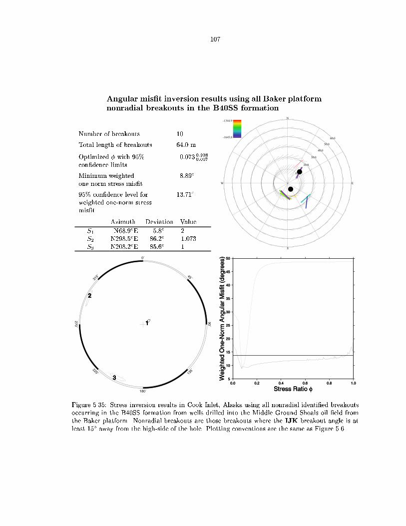
Angular mist inversion results using all Baker platform
nonradial breakouts in the BSS formation
Number of breakouts
Total length of breakouts m
Optimized with condence limits
Minimum weightedonenorm stress mist
condence level forweighted onenorm stressmist
Azimuth Deviation Value
S NE S NE S NE
N
S
EW
10.0
20.0
30.0
40.0
50.0
60.0-1645.8
-1344.9
0˚
315˚
270˚
225˚
180˚
135˚
90˚
45˚
1
2
3
1
2
3
1
2
3 5
10
15
20
25
30
35
40
45
50
Wei
ghte
d O
ne-N
orm
Ang
ular
Mis
fit (
degr
ees)
0.0 0.2 0.4 0.6 0.8 1.0
Stress Ratio φ
5
10
15
20
25
30
35
40
45
50
Wei
ghte
d O
ne-N
orm
Ang
ular
Mis
fit (
degr
ees)
0.0 0.2 0.4 0.6 0.8 1.0
Stress Ratio φ
5
10
15
20
25
30
35
40
45
50
Wei
ghte
d O
ne-N
orm
Ang
ular
Mis
fit (
degr
ees)
0.0 0.2 0.4 0.6 0.8 1.0
Stress Ratio φ
Figure Stress inversion results in Cook Inlet Alaska using all nonradial identied breakoutsoccurring in the BSS formation from wells drilled into the Middle Ground Shoals oil eld fromthe Baker platform Nonradial breakouts are those breakouts where the IJK breakout angle is atleast away from the highside of the hole Plotting conventions are the same as Figure

Stress mist inversion results using all Baker platform
breakouts in the D formation
Number of breakouts
Total length of breakouts m
Optimized with condence limits
Minimum weightedonenorm stress mist
x
condence level forweighted onenorm stressmist
x
Azimuth Deviation Value
S NE S NE S NE
N
S
EW
10.0
20.0
30.0
40.0
50.0
60.0-2205.2
-2002.6
0˚
315˚
270˚
225˚
180˚
135˚
90˚
45˚
1
2
3
1
2
3
1
2
3
0.00
0.05
0.10
0.15
0.20
Wei
ghte
d O
ne-N
orm
Str
ess
Mis
fit
0.0 0.2 0.4 0.6 0.8 1.0
Stress Ratio φ
0.00
0.05
0.10
0.15
0.20
Wei
ghte
d O
ne-N
orm
Str
ess
Mis
fit
0.0 0.2 0.4 0.6 0.8 1.0
Stress Ratio φ
0.00
0.05
0.10
0.15
0.20
Wei
ghte
d O
ne-N
orm
Str
ess
Mis
fit
0.0 0.2 0.4 0.6 0.8 1.0
Stress Ratio φ
Figure Stress inversion results in Cook Inlet Alaska using all identied breakouts occurring inthe D formation from wells drilled into the Middle Ground Shoals oil eld from the Baker platformPlotting conventions are the same as Figure

Angular mist inversion results using all Baker platform
breakouts in the D formation
Number of breakouts
Total length of breakouts m
Optimized with condence limits
Minimum weightedonenorm stress mist
condence level forweighted onenorm stressmist
Azimuth Deviation Value
S NE S NE S NE
N
S
EW
10.0
20.0
30.0
40.0
50.0
60.0-2205.2
-2002.6
0˚
315˚
270˚
225˚
180˚
135˚
90˚
45˚
1
2
3
1
2
3
1
2
3
0
10
20
30
40
50
Wei
ghte
d O
ne-N
orm
Ang
ular
Mis
fit (
degr
ees)
0.0 0.2 0.4 0.6 0.8 1.0
Stress Ratio φ
0
10
20
30
40
50
Wei
ghte
d O
ne-N
orm
Ang
ular
Mis
fit (
degr
ees)
0.0 0.2 0.4 0.6 0.8 1.0
Stress Ratio φ
0
10
20
30
40
50
Wei
ghte
d O
ne-N
orm
Ang
ular
Mis
fit (
degr
ees)
0.0 0.2 0.4 0.6 0.8 1.0
Stress Ratio φ
Figure Stress inversion results in Cook Inlet Alaska using all identied breakouts occurring inthe D formation from wells drilled into the Middle Ground Shoals oil eld from the Baker platformPlotting conventions are the same as Figure

Stress mist inversion results using all Baker platform
nonradial breakouts in the D formation
Number of breakouts
Total length of breakouts m
Optimized with condence limits
Minimum weightedonenorm stress mist
x
condence level forweighted onenorm stressmist
x
Azimuth Deviation Value
S NE S NE S NE
N
S
EW
10.0
20.0
30.0
40.0
50.0
60.0-2205.2
-2002.6
0˚
315˚
270˚
225˚
180˚
135˚
90˚
45˚
1
2
31
2
31
2
3
0.00
0.01
0.02
0.03
0.04
0.05
0.06
0.07
0.08
0.09
Wei
ghte
d O
ne-N
orm
Str
ess
Mis
fit
0.0 0.2 0.4 0.6 0.8 1.0
Stress Ratio φ
0.00
0.01
0.02
0.03
0.04
0.05
0.06
0.07
0.08
0.09
Wei
ghte
d O
ne-N
orm
Str
ess
Mis
fit
0.0 0.2 0.4 0.6 0.8 1.0
Stress Ratio φ
0.00
0.01
0.02
0.03
0.04
0.05
0.06
0.07
0.08
0.09
Wei
ghte
d O
ne-N
orm
Str
ess
Mis
fit
0.0 0.2 0.4 0.6 0.8 1.0
Stress Ratio φ
Figure Stress inversion results in Cook Inlet Alaska using all nonradial identied breakoutsoccurring in the D formation from wells drilled into the Middle Ground Shoals oil eld from theBaker platform Nonradial breakouts are those breakouts where the IJK breakout angle is at least away from the highside of the hole Plotting conventions are the same as Figure

Angular mist inversion results using all Baker platform
nonradial breakouts in the D formation
Number of breakouts
Total length of breakouts m
Optimized with condence limits
Minimum weightedonenorm stress mist
condence level forweighted onenorm stressmist
Azimuth Deviation Value
S NE S NE S NE
N
S
EW
10.0
20.0
30.0
40.0
50.0
60.0-2205.2
-2002.6
0˚
315˚
270˚
225˚
180˚
135˚
90˚
45˚
1
2
3 1
2
3 1
2
3
1
2
3
4
5
6
7
8
9
Wei
ghte
d O
ne-N
orm
Ang
ular
Mis
fit (
degr
ees)
0.0 0.2 0.4 0.6 0.8 1.0
Stress Ratio φ
1
2
3
4
5
6
7
8
9
Wei
ghte
d O
ne-N
orm
Ang
ular
Mis
fit (
degr
ees)
0.0 0.2 0.4 0.6 0.8 1.0
Stress Ratio φ
1
2
3
4
5
6
7
8
9
Wei
ghte
d O
ne-N
orm
Ang
ular
Mis
fit (
degr
ees)
0.0 0.2 0.4 0.6 0.8 1.0
Stress Ratio φ
Figure Stress inversion results in Cook Inlet Alaska using all nonradial identied breakoutsoccurring in the D formation from wells drilled into the Middle Ground Shoals oil eld from theBaker platform Nonradial breakouts are those breakouts where the IJK breakout angle is at least away from the highside of the hole Plotting conventions are the same as Figure

Stress mist inversion results using all Baker platform
breakouts in the G and G formations
Number of breakouts
Total length of breakouts m
Optimized with condence limits
Minimum weightedonenorm stress mist
condence level forweighted onenorm stressmist
Azimuth Deviation Value
S NE S NE S NE
N
S
EW
10.0
20.0
30.0
40.0
50.0
60.0-2768.9
-2410.4
0˚
315˚
270˚
225˚
180˚
135˚
90˚
45˚
1
2
3
1
2
3
1
2
3
0.0
0.1
0.2
0.3
0.4
0.5
Wei
ghte
d O
ne-N
orm
Str
ess
Mis
fit
0.0 0.2 0.4 0.6 0.8 1.0
Stress Ratio φ
0.0
0.1
0.2
0.3
0.4
0.5
Wei
ghte
d O
ne-N
orm
Str
ess
Mis
fit
0.0 0.2 0.4 0.6 0.8 1.0
Stress Ratio φ
0.0
0.1
0.2
0.3
0.4
0.5
Wei
ghte
d O
ne-N
orm
Str
ess
Mis
fit
0.0 0.2 0.4 0.6 0.8 1.0
Stress Ratio φ
Figure Stress inversion results in Cook Inlet Alaska using all identied breakouts occurring inthe G and G formations from wells drilled into the Middle Ground Shoals oil eld from the Bakerplatform Plotting conventions are the same as Figure

Angular mist inversion results using all Baker platform
breakouts in the G and G formations
Number of breakouts
Total length of breakouts m
Optimized with condence limits
Minimum weightedonenorm stress mist
condence level forweighted onenorm stressmist
Azimuth Deviation Value
S NE S NE S NE
N
S
EW
10.0
20.0
30.0
40.0
50.0
60.0-2768.9
-2410.4
0˚
315˚
270˚
225˚
180˚
135˚
90˚
45˚
1
2
3
1
2
3
1
2
3
10
20
30
40
50
Wei
ghte
d O
ne-N
orm
Ang
ular
Mis
fit (
degr
ees)
0.0 0.2 0.4 0.6 0.8 1.0
Stress Ratio φ
10
20
30
40
50
Wei
ghte
d O
ne-N
orm
Ang
ular
Mis
fit (
degr
ees)
0.0 0.2 0.4 0.6 0.8 1.0
Stress Ratio φ
10
20
30
40
50
Wei
ghte
d O
ne-N
orm
Ang
ular
Mis
fit (
degr
ees)
0.0 0.2 0.4 0.6 0.8 1.0
Stress Ratio φ
Figure Stress inversion results in Cook Inlet Alaska using all identied breakouts occurring inthe G and G formations from wells drilled into the Middle Ground Shoals oil eld from the Bakerplatform Plotting conventions are the same as Figure

Stress mist inversion results using all Baker platform
nonradial breakouts in the G and G formations
Number of breakouts
Total length of breakouts m
Optimized with condence limits
Minimum weightedonenorm stress mist
condence level forweighted onenorm stressmist
Azimuth Deviation Value
S NE S NE S NE
N
S
EW
10.0
20.0
30.0
40.0
50.0
60.0-2768.9
-2410.4
0˚
315˚
270˚
225˚
180˚
135˚
90˚
45˚
1
2
3
1
2
3
1
2
3
0.0
0.1
0.2
0.3
0.4
0.5
Wei
ghte
d O
ne-N
orm
Str
ess
Mis
fit
0.0 0.2 0.4 0.6 0.8 1.0
Stress Ratio φ
0.0
0.1
0.2
0.3
0.4
0.5
Wei
ghte
d O
ne-N
orm
Str
ess
Mis
fit
0.0 0.2 0.4 0.6 0.8 1.0
Stress Ratio φ
0.0
0.1
0.2
0.3
0.4
0.5
Wei
ghte
d O
ne-N
orm
Str
ess
Mis
fit
0.0 0.2 0.4 0.6 0.8 1.0
Stress Ratio φ
Figure Stress inversion results in Cook Inlet Alaska using all nonradial identied breakoutsoccurring in the G and G formations from wells drilled into the Middle Ground Shoals oil eldfrom the Baker platform Nonradial breakouts are those breakouts where the IJK breakout angle isat least away from the highside of the hole Plotting conventions are the same as Figure

Angular mist inversion results using all Baker platform
nonradial breakouts in the G and G formations
Number of breakouts
Total length of breakouts m
Optimized with condence limits
Minimum weightedonenorm stress mist
condence level forweighted onenorm stressmist
Azimuth Deviation Value
S NE S NE S NE
N
S
EW
10.0
20.0
30.0
40.0
50.0
60.0-2768.9
-2410.4
0˚
315˚
270˚
225˚
180˚
135˚
90˚
45˚
1
2
3
1
2
3
1
2
3
10
20
30
40
50
Wei
ghte
d O
ne-N
orm
Ang
ular
Mis
fit (
degr
ees)
0.0 0.2 0.4 0.6 0.8 1.0
Stress Ratio φ
10
20
30
40
50
Wei
ghte
d O
ne-N
orm
Ang
ular
Mis
fit (
degr
ees)
0.0 0.2 0.4 0.6 0.8 1.0
Stress Ratio φ
10
20
30
40
50
Wei
ghte
d O
ne-N
orm
Ang
ular
Mis
fit (
degr
ees)
0.0 0.2 0.4 0.6 0.8 1.0
Stress Ratio φ
Figure Stress inversion results in Cook Inlet Alaska using all nonradial identied breakoutsoccurring in the G and G formations from wells drilled into the Middle Ground Shoals oil eldfrom the Baker platform Nonradial breakouts are those breakouts where the IJK breakout angle isat least away from the highside of the hole Plotting conventions are the same as Figure

Stress mist inversion results using all Baker platform
nonradial breakouts between m TVD
Number of breakouts
Total length of breakouts m
Optimized with condence limits
Minimum weightedonenorm stress mist
x
condence level forweighted onenorm stressmist
x
Azimuth Deviation Value
S NE S NE S NE
N
S
EW
10.0
20.0
30.0
40.0
50.0
60.0-1444.9
-1001.8
0˚
315˚
270˚
225˚
180˚
135˚
90˚
45˚
12
3
12
3
12
3
0.00
0.05
0.10
0.15
0.20
0.25
Wei
ghte
d O
ne-N
orm
Str
ess
Mis
fit
0.0 0.2 0.4 0.6 0.8 1.0
Stress Ratio φ
0.00
0.05
0.10
0.15
0.20
0.25
Wei
ghte
d O
ne-N
orm
Str
ess
Mis
fit
0.0 0.2 0.4 0.6 0.8 1.0
Stress Ratio φ
0.00
0.05
0.10
0.15
0.20
0.25
Wei
ghte
d O
ne-N
orm
Str
ess
Mis
fit
0.0 0.2 0.4 0.6 0.8 1.0
Stress Ratio φ
Figure Stress inversion results in Cook Inlet Alaska using all nonradial identied breakoutsbetween and m TVD from wells drilled from the Baker platform in the Middle GroundShoals oil eld Nonradial breakouts are those breakouts where the IJK breakout angle is at least away from the highside of the hole Plotting conventions are the same as Figure

Angular mist inversion results using all Baker platform
nonradial breakouts between m TVD
Number of breakouts
Total length of breakouts m
Optimized with condence limits
Minimum weightedonenorm stress mist
condence level forweighted onenorm stressmist
Azimuth Deviation Value
S NE S NE S NE
N
S
EW
10.0
20.0
30.0
40.0
50.0
60.0-1444.9
-1001.8
0˚
315˚
270˚
225˚
180˚
135˚
90˚
45˚1
2
3
1
2
3
1
2
3
15
20
25
30
35
40
Wei
ghte
d O
ne-N
orm
Ang
ular
Mis
fit (
degr
ees)
0.0 0.2 0.4 0.6 0.8 1.0
Stress Ratio φ
15
20
25
30
35
40
Wei
ghte
d O
ne-N
orm
Ang
ular
Mis
fit (
degr
ees)
0.0 0.2 0.4 0.6 0.8 1.0
Stress Ratio φ
15
20
25
30
35
40
Wei
ghte
d O
ne-N
orm
Ang
ular
Mis
fit (
degr
ees)
0.0 0.2 0.4 0.6 0.8 1.0
Stress Ratio φ
Figure Stress inversion results in Cook Inlet Alaska using all nonradial identied breakoutsbetween and m TVD from wells drilled from the Baker platform in the Middle GroundShoals oil eld Nonradial breakouts are those breakouts where the IJK breakout angle is at least away from the highside of the hole Plotting conventions are the same as Figure

Stress mist inversion results using all Baker platform
nonradial breakouts between m TVD
Number of breakouts
Total length of breakouts m
Optimized with condence limits
Minimum weightedonenorm stress mist
condence level forweighted onenorm stressmist
Azimuth Deviation Value
S NE S NE S NE
N
S
EW
10.0
20.0
30.0
40.0
50.0
60.0-1988.9
-1524.7
0˚
315˚
270˚
225˚
180˚
135˚
90˚
45˚
1
23
1
23
1
23
0.00
0.05
0.10
0.15
Wei
ghte
d O
ne-N
orm
Str
ess
Mis
fit
0.0 0.2 0.4 0.6 0.8 1.0
Stress Ratio φ
0.00
0.05
0.10
0.15
Wei
ghte
d O
ne-N
orm
Str
ess
Mis
fit
0.0 0.2 0.4 0.6 0.8 1.0
Stress Ratio φ
0.00
0.05
0.10
0.15
Wei
ghte
d O
ne-N
orm
Str
ess
Mis
fit
0.0 0.2 0.4 0.6 0.8 1.0
Stress Ratio φ
Figure Stress inversion results in Cook Inlet Alaska using all nonradial identied breakoutsbetween and m TVD from wells drilled from the Baker platform in the Middle GroundShoals oil eld Nonradial breakouts are those breakouts where the IJK breakout angle is at least away from the highside of the hole Plotting conventions are the same as Figure

Angular mist inversion results using all Baker platform
nonradial breakouts between m TVD
Number of breakouts
Total length of breakouts m
Optimized with condence limits
Minimum weightedonenorm stress mist
condence level forweighted onenorm stressmist
Azimuth Deviation Value
S NE S NE S NE
N
S
EW
10.0
20.0
30.0
40.0
50.0
60.0-1988.9
-1524.7
0˚
315˚
270˚
225˚
180˚
135˚
90˚
45˚
1
23
1
23
1
23
0
10
20
30
40
50
60
70
80
Wei
ghte
d O
ne-N
orm
Ang
ular
Mis
fit (
degr
ees)
0.0 0.2 0.4 0.6 0.8 1.0
Stress Ratio φ
0
10
20
30
40
50
60
70
80
Wei
ghte
d O
ne-N
orm
Ang
ular
Mis
fit (
degr
ees)
0.0 0.2 0.4 0.6 0.8 1.0
Stress Ratio φ
0
10
20
30
40
50
60
70
80
Wei
ghte
d O
ne-N
orm
Ang
ular
Mis
fit (
degr
ees)
0.0 0.2 0.4 0.6 0.8 1.0
Stress Ratio φ
Figure Stress inversion results in Cook Inlet Alaska using all nonradial identied breakoutsbetween and m TVD from wells drilled from the Baker platform in the Middle GroundShoals oil eld Nonradial breakouts are those breakouts where the IJK breakout angle is at least away from the highside of the hole Plotting conventions are the same as Figure

Stress mist inversion results using all Baker platform
nonradial breakouts between m TVD
Number of breakouts
Total length of breakouts m
Optimized with condence limits
Minimum weightedonenorm stress mist
condence level forweighted onenorm stressmist
Azimuth Deviation Value
S NE S NE S NE
N
S
EW
10.0
20.0
30.0
40.0
50.0
60.0-2485.6
-2002.6
0˚
315˚
270˚
225˚
180˚
135˚
90˚
45˚
1
2
3
1
2
3
1
2
3
0.00
0.02
0.04
0.06
0.08
0.10
0.12
0.14
0.16
0.18
0.20
0.22
Wei
ghte
d O
ne-N
orm
Str
ess
Mis
fit
0.0 0.2 0.4 0.6 0.8 1.0
Stress Ratio φ
0.00
0.02
0.04
0.06
0.08
0.10
0.12
0.14
0.16
0.18
0.20
0.22
Wei
ghte
d O
ne-N
orm
Str
ess
Mis
fit
0.0 0.2 0.4 0.6 0.8 1.0
Stress Ratio φ
0.00
0.02
0.04
0.06
0.08
0.10
0.12
0.14
0.16
0.18
0.20
0.22
Wei
ghte
d O
ne-N
orm
Str
ess
Mis
fit
0.0 0.2 0.4 0.6 0.8 1.0
Stress Ratio φ
Figure Stress inversion results in Cook Inlet Alaska using all nonradial identied breakoutsbetween and m TVD from wells drilled from the Baker platform in the Middle GroundShoals oil eld Nonradial breakouts are those breakouts where the IJK breakout angle is at least away from the highside of the hole Plotting conventions are the same as Figure

Angular mist inversion results using all Baker platform
nonradial breakouts between m TVD
Number of breakouts
Total length of breakouts m
Optimized with condence limits
Minimum weightedonenorm stress mist
condence level forweighted onenorm stressmist
Azimuth Deviation Value
S NE S NE S NE
N
S
EW
10.0
20.0
30.0
40.0
50.0
60.0-2485.6
-2002.6
0˚
315˚
270˚
225˚
180˚
135˚
90˚
45˚
1
2
3
1
2
3
1
2
3
12
14
16
18
20
22
24
26
28
30
32
Wei
ghte
d O
ne-N
orm
Ang
ular
Mis
fit (
degr
ees)
0.0 0.2 0.4 0.6 0.8 1.0
Stress Ratio φ
12
14
16
18
20
22
24
26
28
30
32
Wei
ghte
d O
ne-N
orm
Ang
ular
Mis
fit (
degr
ees)
0.0 0.2 0.4 0.6 0.8 1.0
Stress Ratio φ
12
14
16
18
20
22
24
26
28
30
32
Wei
ghte
d O
ne-N
orm
Ang
ular
Mis
fit (
degr
ees)
0.0 0.2 0.4 0.6 0.8 1.0
Stress Ratio φ
Figure Stress inversion results in Cook Inlet Alaska using all nonradial identied breakoutsbetween and m TVD from wells drilled from the Baker platform in the Middle GroundShoals oil eld Nonradial breakouts are those breakouts where the IJK breakout angle is at least away from the highside of the hole Plotting conventions are the same as Figure

Stress mist inversion results using all Baker platform
nonradial breakouts between m TVD
Number of breakouts
Total length of breakouts m
Optimized with condence limits
Minimum weightedonenorm stress mist
condence level forweighted onenorm stressmist
Azimuth Deviation Value
S NE S NE S NE
N
S
EW
10.0
20.0
30.0
40.0
50.0
60.0-2768.9
-2515.7
0˚
315˚
270˚
225˚
180˚
135˚
90˚
45˚
1
2
3
1
2
3
1
2
3
0.0
0.1
0.2
0.3
0.4
Wei
ghte
d O
ne-N
orm
Str
ess
Mis
fit
0.0 0.2 0.4 0.6 0.8 1.0
Stress Ratio φ
0.0
0.1
0.2
0.3
0.4
Wei
ghte
d O
ne-N
orm
Str
ess
Mis
fit
0.0 0.2 0.4 0.6 0.8 1.0
Stress Ratio φ
0.0
0.1
0.2
0.3
0.4
Wei
ghte
d O
ne-N
orm
Str
ess
Mis
fit
0.0 0.2 0.4 0.6 0.8 1.0
Stress Ratio φ
Figure Stress inversion results in Cook Inlet Alaska using all nonradial identied breakoutsbetween and m TVD from wells drilled from the Baker platform in the Middle GroundShoals oil eld Nonradial breakouts are those breakouts where the IJK breakout angle is at least away from the highside of the hole Plotting conventions are the same as Figure

Angular mist inversion results using all Baker platform
nonradial breakouts between m TVD
Number of breakouts
Total length of breakouts m
Optimized with condence limits
Minimum weightedonenorm stress mist
condence level forweighted onenorm stressmist
Azimuth Deviation Value
S NE S NE S NE
N
S
EW
10.0
20.0
30.0
40.0
50.0
60.0-2768.9
-2515.7
0˚
315˚
270˚
225˚
180˚
135˚
90˚
45˚
1
2
3
1
2
3
1
2
3
18
20
22
24
26
28
30
32
34
36
38
40
42
Wei
ghte
d O
ne-N
orm
Ang
ular
Mis
fit (
degr
ees)
0.0 0.2 0.4 0.6 0.8 1.0
Stress Ratio φ
18
20
22
24
26
28
30
32
34
36
38
40
42
Wei
ghte
d O
ne-N
orm
Ang
ular
Mis
fit (
degr
ees)
0.0 0.2 0.4 0.6 0.8 1.0
Stress Ratio φ
18
20
22
24
26
28
30
32
34
36
38
40
42
Wei
ghte
d O
ne-N
orm
Ang
ular
Mis
fit (
degr
ees)
0.0 0.2 0.4 0.6 0.8 1.0
Stress Ratio φ
Figure Stress inversion results in Cook Inlet Alaska using all nonradial identied breakoutsbetween and m TVD from wells drilled from the Baker platform in the Middle GroundShoals oil eld Nonradial breakouts are those breakouts where the IJK breakout angle is at least away from the highside of the hole Plotting conventions are the same as Figure

Stress mist inversion results using all Dillon platform
breakouts excluding breakouts from well Smgs
Number of breakouts
Total length of breakouts m
Optimized with condence limits
Minimum weightedonenorm stress mist
condence level forweighted onenorm stressmist
Azimuth Deviation Value
S NE S NE S NE
N
S
EW
10.0
20.0
30.0
40.0
50.0
60.0-3028.5
-948.8
0˚
315˚
270˚
225˚
180˚
135˚
90˚
45˚
1
2
3
1
2
3
1
2
3
0.00
0.02
0.04
0.06
0.08
0.10
0.12
0.14
0.16
0.18
0.20
0.22
Wei
ghte
d O
ne-N
orm
Str
ess
Mis
fit
0.0 0.2 0.4 0.6 0.8 1.0
Stress Ratio φ
0.00
0.02
0.04
0.06
0.08
0.10
0.12
0.14
0.16
0.18
0.20
0.22
Wei
ghte
d O
ne-N
orm
Str
ess
Mis
fit
0.0 0.2 0.4 0.6 0.8 1.0
Stress Ratio φ
0.00
0.02
0.04
0.06
0.08
0.10
0.12
0.14
0.16
0.18
0.20
0.22
Wei
ghte
d O
ne-N
orm
Str
ess
Mis
fit
0.0 0.2 0.4 0.6 0.8 1.0
Stress Ratio φ
Figure Stress inversion results in Cook Inlet Alaska using all identied breakouts from wellsdrilled from the Dillon platform in the Middle Ground Shoals oil eld excluding the breakouts fromwell Smgs Plotting conventions are the same as Figure

Angular mist inversion results using all Dillon platform
breakouts excluding breakouts from well Smgs
Number of breakouts
Total length of breakouts m
Optimized with condence limits
Minimum weightedonenorm stress mist
condence level forweighted onenorm stressmist
Azimuth Deviation Value
S NE S NE S NE
N
S
EW
10.0
20.0
30.0
40.0
50.0
60.0-3028.5
-948.8
0˚
315˚
270˚
225˚
180˚
135˚
90˚
45˚
1
2
3
1
2
3
1
2
3
10
15
20
25
30
35
40
45
50
55
Wei
ghte
d O
ne-N
orm
Ang
ular
Mis
fit (
degr
ees)
0.0 0.2 0.4 0.6 0.8 1.0
Stress Ratio φ
10
15
20
25
30
35
40
45
50
55
Wei
ghte
d O
ne-N
orm
Ang
ular
Mis
fit (
degr
ees)
0.0 0.2 0.4 0.6 0.8 1.0
Stress Ratio φ
10
15
20
25
30
35
40
45
50
55
Wei
ghte
d O
ne-N
orm
Ang
ular
Mis
fit (
degr
ees)
0.0 0.2 0.4 0.6 0.8 1.0
Stress Ratio φ
Figure Stress inversion results in Cook Inlet Alaska using all identied breakouts from wellsdrilled from the Dillon platform in the Middle Ground Shoals oil eld excluding the breakouts fromwell Smgs Plotting conventions are the same as Figure

Stress mist inversion results using all Dillon plat
form nonradial breakouts excluding breakouts from well
Smgs
Number of breakouts
Total length of breakouts m
Optimized with condence limits
Minimum weightedonenorm stress mist
condence level forweighted onenorm stressmist
Azimuth Deviation Value
S NE S NE S NE
N
S
EW
10.0
20.0
30.0
40.0
50.0
60.0-3028.5
-948.8
0˚
315˚
270˚
225˚
180˚
135˚
90˚
45˚
1
2
3
1
2
3
1
2
3
0.0
0.1
0.2
0.3
0.4
Wei
ghte
d O
ne-N
orm
Str
ess
Mis
fit
0.0 0.2 0.4 0.6 0.8 1.0
Stress Ratio φ
0.0
0.1
0.2
0.3
0.4
Wei
ghte
d O
ne-N
orm
Str
ess
Mis
fit
0.0 0.2 0.4 0.6 0.8 1.0
Stress Ratio φ
0.0
0.1
0.2
0.3
0.4
Wei
ghte
d O
ne-N
orm
Str
ess
Mis
fit
0.0 0.2 0.4 0.6 0.8 1.0
Stress Ratio φ
Figure Stress inversion results in Cook Inlet Alaska using all nonradial identied breakoutsfrom wells drilled from the Dillon platform in the Middle Ground Shoals oil eld excluding thebreakouts from well Smgs Nonradial breakouts are those breakouts where the IJK breakout angleis at least away from the highside of the hole Plotting conventions are the same as Figure

Angular mist inversion results using all Dillon plat
form nonradial breakouts excluding breakouts from well
Smgs
Number of breakouts
Total length of breakouts m
Optimized with condence limits
Minimum weightedonenorm stress mist
condence level forweighted onenorm stressmist
Azimuth Deviation Value
S NE S NE S NE
N
S
EW
10.0
20.0
30.0
40.0
50.0
60.0-3028.5
-948.8
0˚
315˚
270˚
225˚
180˚
135˚
90˚
45˚
1
2
3
1
2
3
1
2
3
15
20
25
30
35
40
45
50
55
Wei
ghte
d O
ne-N
orm
Ang
ular
Mis
fit (
degr
ees)
0.0 0.2 0.4 0.6 0.8 1.0
Stress Ratio φ
15
20
25
30
35
40
45
50
55
Wei
ghte
d O
ne-N
orm
Ang
ular
Mis
fit (
degr
ees)
0.0 0.2 0.4 0.6 0.8 1.0
Stress Ratio φ
15
20
25
30
35
40
45
50
55
Wei
ghte
d O
ne-N
orm
Ang
ular
Mis
fit (
degr
ees)
0.0 0.2 0.4 0.6 0.8 1.0
Stress Ratio φ
Figure Stress inversion results in Cook Inlet Alaska using all nonradial identied breakoutsfrom wells drilled from the Dillon platform in the Middle Ground Shoals oil eld excluding thebreakouts from well Smgs Nonradial breakouts are those breakouts where the IJK breakout angleis at least away from the highside of the hole Plotting conventions are the same as Figure

Stress mist inversion results using all Dillon platform
breakouts excluding breakouts from wells Smgs and
Smgs
Number of breakouts
Total length of breakouts m
Optimized with condence limits
Minimum weightedonenorm stress mist
condence level forweighted onenorm stressmist
Azimuth Deviation Value
S NE S NE S NE
N
S
EW
10.0
20.0
30.0
40.0
50.0
60.0-3028.5
-948.8
0˚
315˚
270˚
225˚
180˚
135˚
90˚
45˚
1
2
3
1
2
3
1
2
3
0.00
0.05
0.10
0.15
0.20
0.25
Wei
ghte
d O
ne-N
orm
Str
ess
Mis
fit
0.0 0.2 0.4 0.6 0.8 1.0
Stress Ratio φ
0.00
0.05
0.10
0.15
0.20
0.25
Wei
ghte
d O
ne-N
orm
Str
ess
Mis
fit
0.0 0.2 0.4 0.6 0.8 1.0
Stress Ratio φ
0.00
0.05
0.10
0.15
0.20
0.25
Wei
ghte
d O
ne-N
orm
Str
ess
Mis
fit
0.0 0.2 0.4 0.6 0.8 1.0
Stress Ratio φ
Figure Stress inversion results in Cook Inlet Alaska using all identied breakouts from wellsdrilled from the Dillon platform in the Middle Ground Shoals oil eld excluding the breakouts fromwells Smgs and Smgs Plotting conventions are the same as Figure

Angular mist inversion results using all Dillon platform
breakouts excluding breakouts from wells Smgs and
Smgs
Number of breakouts
Total length of breakouts m
Optimized with condence limits
Minimum weightedonenorm stress mist
condence level forweighted onenorm stressmist
Azimuth Deviation Value
S NE S NE S NE
N
S
EW
10.0
20.0
30.0
40.0
50.0
60.0-3028.5
-948.8
0˚
315˚
270˚
225˚
180˚
135˚
90˚
45˚
1
2
3
1
2
3
1
2
3
10
15
20
25
30
35
40
45
50
55
Wei
ghte
d O
ne-N
orm
Ang
ular
Mis
fit (
degr
ees)
0.0 0.2 0.4 0.6 0.8 1.0
Stress Ratio φ
10
15
20
25
30
35
40
45
50
55
Wei
ghte
d O
ne-N
orm
Ang
ular
Mis
fit (
degr
ees)
0.0 0.2 0.4 0.6 0.8 1.0
Stress Ratio φ
10
15
20
25
30
35
40
45
50
55
Wei
ghte
d O
ne-N
orm
Ang
ular
Mis
fit (
degr
ees)
0.0 0.2 0.4 0.6 0.8 1.0
Stress Ratio φ
Figure Stress inversion results in Cook Inlet Alaska using all identied breakouts from wellsdrilled from the Dillon platform in the Middle Ground Shoals oil eld excluding the breakouts fromwells Smgs and Smgs Plotting conventions are the same as Figure

Stress mist inversion results using all Dillon platform
nonradial breakouts excluding breakouts from wells
Smgs and Smgs
Number of breakouts
Total length of breakouts m
Optimized with condence limits
Minimum weightedonenorm stress mist
condence level forweighted onenorm stressmist
Azimuth Deviation Value
S NE S NE S NE
N
S
EW
10.0
20.0
30.0
40.0
50.0
60.0-3028.5
-948.8
0˚
315˚
270˚
225˚
180˚
135˚
90˚
45˚
1
2
3
1
2
3
1
2
3
0.00
0.05
0.10
0.15
0.20
0.25
0.30
0.35
Wei
ghte
d O
ne-N
orm
Str
ess
Mis
fit
0.0 0.2 0.4 0.6 0.8 1.0
Stress Ratio φ
0.00
0.05
0.10
0.15
0.20
0.25
0.30
0.35
Wei
ghte
d O
ne-N
orm
Str
ess
Mis
fit
0.0 0.2 0.4 0.6 0.8 1.0
Stress Ratio φ
0.00
0.05
0.10
0.15
0.20
0.25
0.30
0.35
Wei
ghte
d O
ne-N
orm
Str
ess
Mis
fit
0.0 0.2 0.4 0.6 0.8 1.0
Stress Ratio φ
Figure Stress inversion results in Cook Inlet Alaska using all nonradial identied breakoutsfrom wells drilled from the Dillon platform in the Middle Ground Shoals oil eld excluding thebreakouts from wells Smgs and Smgs Nonradial breakouts are those breakouts where the IJKbreakout angle is at least away from the highside of the hole Plotting conventions are the sameas Figure
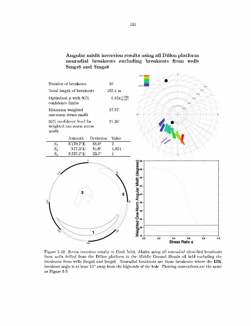
Angular mist inversion results using all Dillon platform
nonradial breakouts excluding breakouts from wells
Smgs and Smgs
Number of breakouts
Total length of breakouts m
Optimized with condence limits
Minimum weightedonenorm stress mist
condence level forweighted onenorm stressmist
Azimuth Deviation Value
S NE S NE S NE
N
S
EW
10.0
20.0
30.0
40.0
50.0
60.0-3028.5
-948.8
0˚
315˚
270˚
225˚
180˚
135˚
90˚
45˚
1
23
1
23
1
23
15
20
25
30
35
40
45
50
55
60
Wei
ghte
d O
ne-N
orm
Ang
ular
Mis
fit (
degr
ees)
0.0 0.2 0.4 0.6 0.8 1.0
Stress Ratio φ
15
20
25
30
35
40
45
50
55
60
Wei
ghte
d O
ne-N
orm
Ang
ular
Mis
fit (
degr
ees)
0.0 0.2 0.4 0.6 0.8 1.0
Stress Ratio φ
15
20
25
30
35
40
45
50
55
60
Wei
ghte
d O
ne-N
orm
Ang
ular
Mis
fit (
degr
ees)
0.0 0.2 0.4 0.6 0.8 1.0
Stress Ratio φ
Figure Stress inversion results in Cook Inlet Alaska using all nonradial identied breakoutsfrom wells drilled from the Dillon platform in the Middle Ground Shoals oil eld excluding thebreakouts from wells Smgs and Smgs Nonradial breakouts are those breakouts where the IJKbreakout angle is at least away from the highside of the hole Plotting conventions are the sameas Figure

Stress mist inversion results using all Dillon platform
breakouts in the TE formation excluding breakouts
from well Smgs
Number of breakouts
Total length of breakouts m
Optimized with condence limits
Minimum weightedonenorm stress mist
x
condence level forweighted onenorm stressmist
x
Azimuth Deviation Value
S NE S NE S NE
N
S
EW
10.0
20.0
30.0
40.0
50.0
60.0-2737
-2693.8
0˚
315˚
270˚
225˚
180˚
135˚
90˚
45˚
12
3
12
3
12
3
0.00
0.02
0.04
0.06
0.08
0.10
0.12
Wei
ghte
d O
ne-N
orm
Str
ess
Mis
fit
0.0 0.2 0.4 0.6 0.8 1.0
Stress Ratio φ
0.00
0.02
0.04
0.06
0.08
0.10
0.12
Wei
ghte
d O
ne-N
orm
Str
ess
Mis
fit
0.0 0.2 0.4 0.6 0.8 1.0
Stress Ratio φ
0.00
0.02
0.04
0.06
0.08
0.10
0.12
Wei
ghte
d O
ne-N
orm
Str
ess
Mis
fit
0.0 0.2 0.4 0.6 0.8 1.0
Stress Ratio φ
Figure Stress inversion results in Cook Inlet Alaska using all identied breakouts occurring inthe TE formation from wells drilled from the Dillon platform in the Middle Ground Shoals oil eldexcluding the breakouts from well Smgs Plotting conventions are the same as Figure

Angular mist inversion results using all Dillon plat
form breakouts in the TE formation excluding break
outs from well Smgs
Number of breakouts
Total length of breakouts m
Optimized with condence limits
Minimum weightedonenorm stress mist
condence level forweighted onenorm stressmist
Azimuth Deviation Value
S NE S NE S NE
N
S
EW
10.0
20.0
30.0
40.0
50.0
60.0-2737
-2693.8
0˚
315˚
270˚
225˚
180˚
135˚
90˚
45˚
1
2
3 1
2
3 1
2
3
0
10
20
30
40
50
Wei
ghte
d O
ne-N
orm
Ang
ular
Mis
fit (
degr
ees)
0.0 0.2 0.4 0.6 0.8 1.0
Stress Ratio φ
0
10
20
30
40
50
Wei
ghte
d O
ne-N
orm
Ang
ular
Mis
fit (
degr
ees)
0.0 0.2 0.4 0.6 0.8 1.0
Stress Ratio φ
0
10
20
30
40
50
Wei
ghte
d O
ne-N
orm
Ang
ular
Mis
fit (
degr
ees)
0.0 0.2 0.4 0.6 0.8 1.0
Stress Ratio φ
Figure Stress inversion results in Cook Inlet Alaska using all identied breakouts occurring inthe TE formation from wells drilled from the Dillon platform in the Middle Ground Shoals oil eldexcluding the breakouts from well Smgs Plotting conventions are the same as Figure

Stress mist inversion results using all Dillon platform
nonradial breakouts between m TVD ex
cluding breakouts from well Smgs
Number of breakouts
Total length of breakouts m
Optimized with condence limits
Minimum weightedonenorm stress mist
x
condence level forweighted onenorm stressmist
x
Azimuth Deviation Value
S NE S NE S NE
N
S
EW
10.0
20.0
30.0
40.0
50.0
60.0-1931.7
-1503.5
0˚
315˚
270˚
225˚
180˚
135˚
90˚
45˚
1
2
3
1
2
3
1
2
3
0.0
0.1
0.2
0.3
0.4
0.5
Wei
ghte
d O
ne-N
orm
Str
ess
Mis
fit
0.0 0.2 0.4 0.6 0.8 1.0
Stress Ratio φ
0.0
0.1
0.2
0.3
0.4
0.5
Wei
ghte
d O
ne-N
orm
Str
ess
Mis
fit
0.0 0.2 0.4 0.6 0.8 1.0
Stress Ratio φ
0.0
0.1
0.2
0.3
0.4
0.5
Wei
ghte
d O
ne-N
orm
Str
ess
Mis
fit
0.0 0.2 0.4 0.6 0.8 1.0
Stress Ratio φ
Figure Stress inversion results in Cook Inlet Alaska using all nonradial identied breakoutsbetween and m TVD from wells drilled from the Dillon platform in the Middle GroundShoals oil eld excluding the breakouts from well Smgs Nonradial breakouts are those breakoutswhere the IJK breakout angle is at least away from the highside of the hole Plotting conventionsare the same as Figure

Angular mist inversion results using all Dillon plat
form nonradial breakouts between m TVD
excluding breakouts from well Smgs
Number of breakouts
Total length of breakouts m
Optimized with condence limits
Minimum weightedonenorm stress mist
condence level forweighted onenorm stressmist
Azimuth Deviation Value
S NE S NE S NE
N
S
EW
10.0
20.0
30.0
40.0
50.0
60.0-1931.7
-1503.5
0˚
315˚
270˚
225˚
180˚
135˚
90˚
45˚
3
1
23
1
23
1
2
5
10
15
20
25
30
35
Wei
ghte
d O
ne-N
orm
Ang
ular
Mis
fit (
degr
ees)
0.0 0.2 0.4 0.6 0.8 1.0
Stress Ratio φ
5
10
15
20
25
30
35
Wei
ghte
d O
ne-N
orm
Ang
ular
Mis
fit (
degr
ees)
0.0 0.2 0.4 0.6 0.8 1.0
Stress Ratio φ
5
10
15
20
25
30
35
Wei
ghte
d O
ne-N
orm
Ang
ular
Mis
fit (
degr
ees)
0.0 0.2 0.4 0.6 0.8 1.0
Stress Ratio φ
Figure Stress inversion results in Cook Inlet Alaska using all nonradial identied breakoutsbetween and m TVD from wells drilled from the Dillon platform in the Middle GroundShoals oil eld excluding the breakouts from well Smgs Nonradial breakouts are those breakoutswhere the IJK breakout angle is at least away from the highside of the hole Plotting conventionsare the same as Figure

Stress mist inversion results using all Dillon platform
nonradial breakouts between m TVD ex
cluding breakouts from well Smgs
Number of breakouts
Total length of breakouts m
Optimized with condence limits
Minimum weightedonenorm stress mist
x
condence level forweighted onenorm stressmist
x
Azimuth Deviation Value
S NE S NE S NE
N
S
EW
10.0
20.0
30.0
40.0
50.0
60.0-2444.4
-2011.7
0˚
315˚
270˚
225˚
180˚
135˚
90˚
45˚
1
23
1
23
1
23
0.0
0.1
0.2
0.3
0.4
0.5
Wei
ghte
d O
ne-N
orm
Str
ess
Mis
fit
0.0 0.2 0.4 0.6 0.8 1.0
Stress Ratio φ
0.0
0.1
0.2
0.3
0.4
0.5
Wei
ghte
d O
ne-N
orm
Str
ess
Mis
fit
0.0 0.2 0.4 0.6 0.8 1.0
Stress Ratio φ
0.0
0.1
0.2
0.3
0.4
0.5
Wei
ghte
d O
ne-N
orm
Str
ess
Mis
fit
0.0 0.2 0.4 0.6 0.8 1.0
Stress Ratio φ
Figure Stress inversion results in Cook Inlet Alaska using all nonradial identied breakoutsbetween and m TVD from wells drilled from the Dillon platform in the Middle GroundShoals oil eld excluding the breakouts from well Smgs Nonradial breakouts are those breakoutswhere the IJK breakout angle is at least away from the highside of the hole Plotting conventionsare the same as Figure

Angular mist inversion results using all Dillon plat
form nonradial breakouts between m TVD
excluding breakouts from well Smgs
Number of breakouts
Total length of breakouts m
Optimized with condence limits
Minimum weightedonenorm stress mist
condence level forweighted onenorm stressmist
Azimuth Deviation Value
S NE S NE S NE
N
S
EW
10.0
20.0
30.0
40.0
50.0
60.0-2444.4
-2011.7
0˚
315˚
270˚
225˚
180˚
135˚
90˚
45˚
1
23
1
23
1
23
10
20
30
40
50
Wei
ghte
d O
ne-N
orm
Ang
ular
Mis
fit (
degr
ees)
0.0 0.2 0.4 0.6 0.8 1.0
Stress Ratio φ
10
20
30
40
50
Wei
ghte
d O
ne-N
orm
Ang
ular
Mis
fit (
degr
ees)
0.0 0.2 0.4 0.6 0.8 1.0
Stress Ratio φ
10
20
30
40
50
Wei
ghte
d O
ne-N
orm
Ang
ular
Mis
fit (
degr
ees)
0.0 0.2 0.4 0.6 0.8 1.0
Stress Ratio φ
Figure Stress inversion results in Cook Inlet Alaska using all nonradial identied breakoutsbetween and m TVD from wells drilled from the Dillon platform in the Middle GroundShoals oil eld excluding the breakouts from well Smgs Nonradial breakouts are those breakoutswhere the IJK breakout angle is at least away from the highside of the hole Plotting conventionsare the same as Figure

Stress mist inversion results using all Dillon platform
nonradial breakouts between m TVD ex
cluding breakouts from well Smgs
Number of breakouts
Total length of breakouts m
Optimized with condence limits
Minimum weightedonenorm stress mist
x
condence level forweighted onenorm stressmist
x
Azimuth Deviation Value
S NE S NE S NE
N
S
EW
10.0
20.0
30.0
40.0
50.0
60.0-2955.4
-2588.1
0˚
315˚
270˚
225˚
180˚
135˚
90˚
45˚
1
2
3
1
2
3
1
2
3
0.00
0.01
0.02
0.03
0.04
0.05
0.06
Wei
ghte
d O
ne-N
orm
Str
ess
Mis
fit
0.0 0.2 0.4 0.6 0.8 1.0
Stress Ratio φ
0.00
0.01
0.02
0.03
0.04
0.05
0.06
Wei
ghte
d O
ne-N
orm
Str
ess
Mis
fit
0.0 0.2 0.4 0.6 0.8 1.0
Stress Ratio φ
0.00
0.01
0.02
0.03
0.04
0.05
0.06
Wei
ghte
d O
ne-N
orm
Str
ess
Mis
fit
0.0 0.2 0.4 0.6 0.8 1.0
Stress Ratio φ
Figure Stress inversion results in Cook Inlet Alaska using all nonradial identied breakoutsbetween and m TVD from wells drilled from the Dillon platform in the Middle GroundShoals oil eld excluding the breakouts from well Smgs Nonradial breakouts are those breakoutswhere the IJK breakout angle is at least away from the highside of the hole Plotting conventionsare the same as Figure

Angular mist inversion results using all Dillon plat
form nonradial breakouts between m TVD
excluding breakouts from well Smgs
Number of breakouts
Total length of breakouts m
Optimized with condence limits
Minimum weightedonenorm stress mist
condence level forweighted onenorm stressmist
Azimuth Deviation Value
S NE S NE S NE
N
S
EW
10.0
20.0
30.0
40.0
50.0
60.0-2955.4
-2588.1
0˚
315˚
270˚
225˚
180˚
135˚
90˚
45˚
1
2
3
1
2
3
1
2
3
0
10
20
30
40
50
60
70
Wei
ghte
d O
ne-N
orm
Ang
ular
Mis
fit (
degr
ees)
0.0 0.2 0.4 0.6 0.8 1.0
Stress Ratio φ
0
10
20
30
40
50
60
70
Wei
ghte
d O
ne-N
orm
Ang
ular
Mis
fit (
degr
ees)
0.0 0.2 0.4 0.6 0.8 1.0
Stress Ratio φ
0
10
20
30
40
50
60
70
Wei
ghte
d O
ne-N
orm
Ang
ular
Mis
fit (
degr
ees)
0.0 0.2 0.4 0.6 0.8 1.0
Stress Ratio φ
Figure Stress inversion results in Cook Inlet Alaska using all nonradial identied breakoutsbetween and m TVD from wells drilled from the Dillon platform in the Middle GroundShoals oil eld excluding the breakouts from well Smgs Nonradial breakouts are those breakoutswhere the IJK breakout angle is at least away from the highside of the hole Plotting conventionsare the same as Figure
Stress State Analyses
Granite Point Oil Field Inversion
Eight separate inversions of subsets of the Granite Point breakouts excluding the breakouts from
Gp were performed These subsets were all of the breakouts Figures and nonradial
breakouts Figures and nonradial breakouts between and m TVD Figures
and and nonradial breakouts between and m TVD Figures and All of
the stress and angular mist inversion results have the maximum principal stress direction oriented
subhorizontally NNWSSE in a thrust faulting stress state with a large value S consistently
plunges slightly to the NNW except for the inversions of the nonradial breakouts between
and m TVD where S plunges to the SSE The S and S principal stresses are also
fairly consistently oriented between the di erent inversion results S is consistently oriented near
the vertical and S is oriented ENEWSW The stress state values from the various mists range
from to These data suggest that a thrustfaulting stress state with S oriented in a
NNESSW sense is responsible for these breakout orientations
The Granite Point TXSS marker was initially identied as the marker containing the most
identied Granite Point breakouts All but one of the TXSS breakouts were identied in Gp
Since the breakouts from Gp were not included in the inversion of the Granite Point data due
to inconsistent breakout orientations Section B no inversions of breakouts occurring in Granite
Point marker horizons were performed An examination of other potential markers for study did
not yield any markers containing a large number of breakouts
The irregular condence limits in the angular mist inversion of the nonradial breakouts
and nonradial breakouts between and m TVD are due to two separate distinct mist
minima below the mist condence limit Figures and Since both minima are less
than the condence limit the inversion results are extremely poor The stress mist inversions
also identied similar local minima Figures and but in the case of the stress mist local
minima only one fell within the condence mist limit for each inversion
A comparison of stress mist inversion results for two depth ranges m and
m TVD is shown in Figure The two stress states are visually distinct from each other
However both S azimuths are in sector dened by NNWSSE and NWSE directed azimuths and
the S axes are nearly vertically oriented Michael and Julian developed a method to calculate
the rotation axis and angle of rotation needed to align one set of principal stress axes with another
A rotation of around an axis trending NE and plunging brings the shallower stress
state in alignment with the deeper one The upper to m TVD depth range identied
a nearly degenerate thrust faulting stress state with S striking NW the
condence limits on S allow its azimuth to vary from NW to NW The deeper breakouts
identied from to m TVD were best t by a less degenerate thrust faulting
stress state with the S azimuth more northerly oriented at NW the condence limits on
S allow its azimuth to vary from NW to NW
The best tting stress state theoretical breakout pattern for all of the Granite Point breakouts
and the breakout pattern for the nonradial breakouts visually agree Figures All four
inversions placed breakout nodal points at orientations plunging to the north and to the south of the
breakout data to t the more variably oriented breakouts The stress mist inversion of the complete
Granite Point data set Figure including the radial breakouts is taken as the inversion that
best represents the Granite Point stress state This thrust faulting stress state has S oriented
NW plunging the condence limits allow the azimuth to vary from NW to
NE and the plunge to vary from to The optimized is
Baker Platform Inversion
Twentyfour separate inversions were done of various subsets of breakouts identied from wells drilled
from the Baker platform Eight inversions were performed of nonradial breakouts separated into
m TVD zones from to m Figures Figure plots a vertical prole of
the stress mist nonradial breakout inversion results The stress mist S azimuth over the m
TVD depth interval is oriented in a NNWSSE to NWSE sector NW m TVD
NE m TVD NE m TVD and NE m
TVD The S azimuth in the shallowest interval is essentially unconstrained condence limits
allow S to vary fromNW to NE due to a degenerate stress eld The S azimuth
in the three deeper depth intervals is much better constrained NENE m
TVD NENE m TVD and NENE Over the same depth
interval the plunge of the maximum principal stress direction rotated from plunging north
m TVD to plunging south m TVD south m
TVD and lastly south m TVD
The largest change in stress state as a function of depth is the switch from an almost degenerate
thrust faulting stress state in the to m TVD depth range to a normal faulting stress
state in the to m TVD depth range and a return to the nearly degenerate thrust faulting
from to m TVD Figure In the same normal stress state region is a change from a
NNWSSE directed SH and S orientation to a ENEWSW directed SH and S orientation Along
the same depth interval the stress state ratio moves from to to to For
each depth interval the stress state results from the angular mist inversion are almost identical to
the stress mist inversion results suggesting that the normal faulting stress state observed in the
to m TVD is not an artifact of the inversion The data from to m TVD also
contained the largest number of identied breakouts the second longest total length of breakouts

m TVDFigure
n l m
0˚
315˚
270˚
225˚
180˚
135˚
90˚
45˚
1
2
3
1
2
3
1
2
3
0.00
0.05
0.10
0.15
0.20
Wei
ghte
d O
ne-N
orm
Str
ess
Mis
fit
0.0 0.2 0.4 0.6 0.8 1.0
Stress Ratio φ
0.00
0.05
0.10
0.15
0.20
Wei
ghte
d O
ne-N
orm
Str
ess
Mis
fit
0.0 0.2 0.4 0.6 0.8 1.0
Stress Ratio φ
0.00
0.05
0.10
0.15
0.20
Wei
ghte
d O
ne-N
orm
Str
ess
Mis
fit
0.0 0.2 0.4 0.6 0.8 1.0
Stress Ratio φ
m TVDFigure
n l m
0˚
315˚
270˚
225˚
180˚
135˚
90˚
45˚
1
2
3
1
2
3
1
2
3
0.0
0.1
0.2
0.3
0.4
Wei
ghte
d O
ne-N
orm
Str
ess
Mis
fit
0.0 0.2 0.4 0.6 0.8 1.0
Stress Ratio φ
0.0
0.1
0.2
0.3
0.4
Wei
ghte
d O
ne-N
orm
Str
ess
Mis
fit
0.0 0.2 0.4 0.6 0.8 1.0
Stress Ratio φ
0.0
0.1
0.2
0.3
0.4
Wei
ghte
d O
ne-N
orm
Str
ess
Mis
fit
0.0 0.2 0.4 0.6 0.8 1.0
Stress Ratio φ
Figure Depth variation of the nonradial Granite Point stress mist stress inversion resultsleft The gure number refers to the gure containing all of the plots and information regardingthis inversion n is the number of breakouts and l is the total length of the n breakouts in theinversion middle Lower hemisphere stereographic projection plot where the digits and show the optimized orientation of the S S and S principal stress axes respectively The weighted onenorm mist condence limits of the S S and S orientations are plotted as thicksolid lines thin solid lines and dotted lines respectively The stress state ratio was held constantat the minimum of the mist versus curve on the right right The weighted onenorm mistfor the breakouts as a function of where the thick solid line is the minimized mist when isheld constant and the principal stress directions are unconstrained and the dotted line is the mistusing the principal stress directions from the best tting model A rotation of around an axistrending NE and plunging is required to bring the shallower stress state in alignmentwith the deeper one

m TVDFigure
n l m
0˚
315˚
270˚
225˚
180˚
135˚
90˚
45˚
12
3
12
3
12
3
0.00
0.05
0.10
0.15
0.20
0.25
Wei
ghte
d O
ne-N
orm
Str
ess
Mis
fit
0.0 0.2 0.4 0.6 0.8 1.0
Stress Ratio φ
0.00
0.05
0.10
0.15
0.20
0.25
Wei
ghte
d O
ne-N
orm
Str
ess
Mis
fit
0.0 0.2 0.4 0.6 0.8 1.0
Stress Ratio φ
0.00
0.05
0.10
0.15
0.20
0.25
Wei
ghte
d O
ne-N
orm
Str
ess
Mis
fit
0.0 0.2 0.4 0.6 0.8 1.0
Stress Ratio φ
m TVDFigure
n l m
0˚
315˚
270˚
225˚
180˚
135˚
90˚
45˚
1
23
1
23
1
23
0.00
0.05
0.10
0.15
Wei
ghte
d O
ne-N
orm
Str
ess
Mis
fit
0.0 0.2 0.4 0.6 0.8 1.0
Stress Ratio φ
0.00
0.05
0.10
0.15
Wei
ghte
d O
ne-N
orm
Str
ess
Mis
fit
0.0 0.2 0.4 0.6 0.8 1.0
Stress Ratio φ
0.00
0.05
0.10
0.15
Wei
ghte
d O
ne-N
orm
Str
ess
Mis
fit
0.0 0.2 0.4 0.6 0.8 1.0
Stress Ratio φ
m TVDFigure
n l m
0˚
315˚
270˚
225˚
180˚
135˚
90˚
45˚
1
2
3
1
2
3
1
2
3
0.00
0.02
0.04
0.06
0.08
0.10
0.12
0.14
0.16
0.18
0.20
0.22
Wei
ghte
d O
ne-N
orm
Str
ess
Mis
fit
0.0 0.2 0.4 0.6 0.8 1.0
Stress Ratio φ
0.00
0.02
0.04
0.06
0.08
0.10
0.12
0.14
0.16
0.18
0.20
0.22
Wei
ghte
d O
ne-N
orm
Str
ess
Mis
fit
0.0 0.2 0.4 0.6 0.8 1.0
Stress Ratio φ
0.00
0.02
0.04
0.06
0.08
0.10
0.12
0.14
0.16
0.18
0.20
0.22
Wei
ghte
d O
ne-N
orm
Str
ess
Mis
fit
0.0 0.2 0.4 0.6 0.8 1.0
Stress Ratio φ
m TVDFigure
n l m
0˚
315˚
270˚
225˚
180˚
135˚
90˚
45˚
1
2
3
1
2
3
1
2
3
0.0
0.1
0.2
0.3
0.4
Wei
ghte
d O
ne-N
orm
Str
ess
Mis
fit
0.0 0.2 0.4 0.6 0.8 1.0
Stress Ratio φ
0.0
0.1
0.2
0.3
0.4
Wei
ghte
d O
ne-N
orm
Str
ess
Mis
fit
0.0 0.2 0.4 0.6 0.8 1.0
Stress Ratio φ
0.0
0.1
0.2
0.3
0.4
Wei
ghte
d O
ne-N
orm
Str
ess
Mis
fit
0.0 0.2 0.4 0.6 0.8 1.0
Stress Ratio φ
Figure Depth variation of the nonradial Baker Platform stress mist stress inversion resultsThe S and S condence contours in the m TVD depth range are almost identicaland plot on top of each other Plotting conventions are the same as in Figure

and had a better data distribution so the normal faulting stress state is probably not a sampling
problem No similar changes in stress state occur as a function of depth in either the Granite Point
or Dillon platform breakouts
The breakouts occurring in the selected BSS D G and G markers come from the same
set of breakouts used in the inversions of breakouts separated into m intervals The BSS
marker spans the TVD range to m D spans to m and G combined with
G spans to m TVD As a group the stress state results from inversions of breakouts
and nonradial breakouts occurring in the BSS Figures D Figures and G
combined with G Figures markers are highly inconsistent Stress states determined
using the stress di erence and angular di erence inversions were markedly di erent in four out of
the six marker horizon data sets inverted compare Figure with with with
and with The angular mist inversion yielded signicantly di erent stress state
results when radial breakouts were included in the inversion compare Figure with
with and with However stress states determined from the stress mist inversion of
complete sets of borehole breakouts were highly consistent with the stress states determined from
the nonradial breakouts compare Figure with with and with If only
the stress mist inversion results are considered then overall the data indicate nearly degenerate
thrust faulting stress states where S is within of vertical and S is unconstrained to rotate
about the S axes or oriented clockwise of EW and counterclockwise of NS
Figure compares the stress state results from the nonradial subset of breakouts identied
in each marker The nonradial breakouts from the BSS and the D markers are best t by almost
identical nearly degenerate thrust faulting stress states only a rotation around an axis trending
NE and plunging is required to bring these two stress states into coincidence The
of rotation is the among the smallest amounts of rotation needed to align two stress tensors that has
been observed in any of these data subsets The similarity of the inversion results from these two
distinct sets of breakouts suggests that the stress state is real The BSS S azimuth NE
and the D S azimuth NE are within of each other The breakouts from the G and G
markers appear to have been generated from a nearly degenerate thrust faulting stress state where
S trends NE The consistent ESENNW S azimuth of the BSS and the D markers is
almost perpendicular to the NE striking trend of the Middle Ground Shoal anticline suggesting
that these breakouts may be related to the growth of the anticline and not the regional tectonic
stresses which may control the G and G breakouts This change in stress states occurs between
the m TVD of the deepest D breakout and the m TVD of the shallow G breakout
The breakouts in the D marker and in the G and G markers overlap to some extent the break
outs in the m TVD depth interval where a normal faulting stress state was identied
However none of the inversions of breakouts in these particular markers identied a similar normal

BSS marker m TVDFigure
n l m
0˚
315˚
270˚
225˚
180˚
135˚
90˚
45˚
1
2
3
1
2
3
1
2
3
0.0
0.1
0.2
0.3
0.4
0.5
Wei
ghte
d O
ne-N
orm
Str
ess
Mis
fit
0.0 0.2 0.4 0.6 0.8 1.0
Stress Ratio φ
0.0
0.1
0.2
0.3
0.4
0.5
Wei
ghte
d O
ne-N
orm
Str
ess
Mis
fit
0.0 0.2 0.4 0.6 0.8 1.0
Stress Ratio φ
0.0
0.1
0.2
0.3
0.4
0.5
Wei
ghte
d O
ne-N
orm
Str
ess
Mis
fit
0.0 0.2 0.4 0.6 0.8 1.0
Stress Ratio φ
D marker m TVDFigure
n l m
0˚
315˚
270˚
225˚
180˚
135˚
90˚
45˚
1
2
31
2
31
2
3
0.00
0.01
0.02
0.03
0.04
0.05
0.06
0.07
0.08
0.09
Wei
ghte
d O
ne-N
orm
Str
ess
Mis
fit
0.0 0.2 0.4 0.6 0.8 1.0
Stress Ratio φ
0.00
0.01
0.02
0.03
0.04
0.05
0.06
0.07
0.08
0.09
Wei
ghte
d O
ne-N
orm
Str
ess
Mis
fit
0.0 0.2 0.4 0.6 0.8 1.0
Stress Ratio φ
0.00
0.01
0.02
0.03
0.04
0.05
0.06
0.07
0.08
0.09
Wei
ghte
d O
ne-N
orm
Str
ess
Mis
fit
0.0 0.2 0.4 0.6 0.8 1.0
Stress Ratio φ
Between D and G m TVD
n l m
0˚
315˚
270˚
225˚
180˚
135˚
90˚
45˚
1
2
3
1
2
3
1
2
3
0.00
0.05
0.10
0.15
0.20
0.25
0.30
0.35
Wei
ghte
d O
ne-N
orm
Str
ess
Mis
fit
0.0 0.2 0.4 0.6 0.8 1.0
Stress Ratio φ
0.00
0.05
0.10
0.15
0.20
0.25
0.30
0.35
Wei
ghte
d O
ne-N
orm
Str
ess
Mis
fit
0.0 0.2 0.4 0.6 0.8 1.0
Stress Ratio φ
0.00
0.05
0.10
0.15
0.20
0.25
0.30
0.35
Wei
ghte
d O
ne-N
orm
Str
ess
Mis
fit
0.0 0.2 0.4 0.6 0.8 1.0
Stress Ratio φ
G and G markers m TVDFigure
n l m
0˚
315˚
270˚
225˚
180˚
135˚
90˚
45˚
1
2
3
1
2
3
1
2
3
0.0
0.1
0.2
0.3
0.4
0.5
Wei
ghte
d O
ne-N
orm
Str
ess
Mis
fit
0.0 0.2 0.4 0.6 0.8 1.0
Stress Ratio φ
0.0
0.1
0.2
0.3
0.4
0.5
Wei
ghte
d O
ne-N
orm
Str
ess
Mis
fit
0.0 0.2 0.4 0.6 0.8 1.0
Stress Ratio φ
0.0
0.1
0.2
0.3
0.4
0.5
Wei
ghte
d O
ne-N
orm
Str
ess
Mis
fit
0.0 0.2 0.4 0.6 0.8 1.0
Stress Ratio φ
Figure Comparison of nonradial Baker Platform stress mist stress inversion results frombreakouts occurring in di erent markers and between the D and G markers The true verticaldepth range shown for each marker shows the maximum vertical extent of the breakouts from eachmarker Breakouts not in the marker but within the depth range are not included A rotationof around an axis trending NE and plunging is required to bring the stress statedetermined by the BSS breakouts into alignment with the stress state from the breakouts identiedin the D marker Plotting conventions are the same as in Figure

faulting stress state A stress mist inversion of the nonradial breakouts between and m
TVD excluding those breakouts above and inside the D marker and below and inside the G marker
was performed The stress state determined from this set of breakouts was also a normal faulting
stress state very similar to the m TVD breakout inversion This suggests that as a
function of depth the shallowest stress state is related to the local structure of the anticline then
an anomalous normal faulting stress state is observed at the next deeper level and at the deepest
level the regional stress state is measured
Inversion of all of the Baker breakouts and the nonradial Baker breakouts yielded substantially
di erent stress tensors Figures Both the stress mist and the angular mist inversions
yielded similar stress state results for each data set The stress mist inversion of the complete
Baker platform breakouts identied a nearly degenerate thrust faulting stress state with
S plunging southward at an azimuth of NE The stress state generated by the stress
mist inversion of the nonradial borehole breakouts identied a normal faulting stress state with
near It appears that the nonradial breakout inversion was controlled by the same nonradial
breakouts that generated the normal faulting stress state in the to m TVD depth range
Because the normal faulting stress state was shown to arise in a particular depth range the stress
state results using the complete set of Baker platform breakouts is considered as the stress state
indicative of the volume sampled by the Baker wells Figure This stress state has S plunging
southward at an azimuth of NE with S nearly vertical The condence limits on
S allow its azimuth to vary from NE to NE and its plunge to vary from to
Dillon Platform Inversion
Except for a single breakout identied in the northeastward plunging Smgs well all breakouts from
the Dillon platform were identied in south to westplunging sections of borehole Figure
The breakouts in the southwestplunging boreholes are very consistently oriented in a general NS
to NESW direction
Sixteen separate inversions were performed on subsets of the Dillon platform breakouts The rst
set of inversions are of seven breakouts identied in the TE marker Figures and Three
of these seven breakouts are nonradial Three breakouts cannot constrain a stress tensor and hence
no inversion of the nonradial TE breakouts was performed The inversion of all seven breakouts
yielded an extremely small weighted stress mist of x and a small weighted angular mist
of for these data The small mists were obtained since the seven breakouts in TE are located
in two localized regions on the borehole azimuth and deviation space Figure which limits the
inversion to e ectively inverting for two breakouts The inversions placed a breakout nodal point
on top of the breakouts identied in the more westerly plunging drillhole The resolved stress state
from the stress mist inversion is nearly degenerate thrust faulting with the S azimuth

at NE The angular mist inversion stress results agree closely with the stress mist inversion
results This orientation of the maximum horizontal principal stress is midway between the NNW
SSE SH stress direction and an orientation perpendicular to the NE strike of the Middle Ground
Shoals oil eld
Three m true vertical depth intervals contained a large number of identied nonradial break
outs between and m TVD there were breakouts totaling m in length Figures
and between and m TVD there were breakouts totaling m in length Fig
ures and and between and m TVD there were breakouts totaling m
in length Figures and The three stress mist inversions from to m TVD
exhibit extremely small principal stress direction condence regions Figure Given that
the breakout pattern nodal points were preferentially placed near the moderately deviated breakouts
and that the breakouts occupied a very limited amount of borehole azimuth and deviation space the
inversions yielded nearly degenerate normal faulting stress states with S deviating nearly away
from vertical Given the extremely limited coverage of borehole azimuth and deviation covered by
the breakouts separated into m intervals these inversion results will not be considered as repre
sentative of the stress state in the depth intervals While the number of breakouts in these intervals
is equal to or larger than the number of breakouts performed in the m TVD depth intervals from
the Baker platform the Baker platform breakouts cover a much larger range in borehole azimuth
and deviation space and hence the Baker platform results are considered to be more reliable and
were included in the conclusions about the Baker stress state Finally because the breakouts from
the Dillon platform are in boreholes deviating roughly away from the vertical these breakouts
will not be considered as indicators of the maximum horizontal principal stress direction SH
In contrast to the TE and m TVD depth interval breakout subsets the nonradial and
the radial combined with the nonradial breakout subsets have a large number of breakouts and a
large variation in borehole azimuth and borehole deviation The stress and angular mist inversion
results for all Dillon breakouts and all nonradial Dillon breakouts are not consistent Figures
The substantial di erences between these inversions stems from the single nonradial Smgs
breakout Only one breakout was identied in Smgs in a noisy section of the fourarm dipmeter
caliper curves this suggests that inversions should be performed of the data without this breakout
Figure B Figures show the stress and angular mist inversions of the same complete
and nonradial data sets excluding the Smgs breakout The stress mist inversion results generated
from the complete set of breakouts excluding Smgs and the nonradial breakouts excluding Smgs
are very consistent Figures and requiring only a rotation around an axis trending
NE plunging to align the principal stress directions The stress state generated from the
complete set of breakouts excluding Smgs is only slightly di erent than the stress state including
Smgs Figures and a rotation of the principal stress axes around a horizontal axis

m TVDFigure
n l m
0˚
315˚
270˚
225˚
180˚
135˚
90˚
45˚
1
2
3
1
2
3
1
2
3
0.0
0.1
0.2
0.3
0.4
0.5
Wei
ghte
d O
ne-N
orm
Str
ess
Mis
fit
0.0 0.2 0.4 0.6 0.8 1.0
Stress Ratio φ
0.0
0.1
0.2
0.3
0.4
0.5
Wei
ghte
d O
ne-N
orm
Str
ess
Mis
fit
0.0 0.2 0.4 0.6 0.8 1.0
Stress Ratio φ
0.0
0.1
0.2
0.3
0.4
0.5
Wei
ghte
d O
ne-N
orm
Str
ess
Mis
fit
0.0 0.2 0.4 0.6 0.8 1.0
Stress Ratio φ
m TVDFigure
n l m
0˚
315˚
270˚
225˚
180˚
135˚
90˚
45˚
1
23
1
23
1
23
0.0
0.1
0.2
0.3
0.4
0.5
Wei
ghte
d O
ne-N
orm
Str
ess
Mis
fit
0.0 0.2 0.4 0.6 0.8 1.0
Stress Ratio φ
0.0
0.1
0.2
0.3
0.4
0.5
Wei
ghte
d O
ne-N
orm
Str
ess
Mis
fit
0.0 0.2 0.4 0.6 0.8 1.0
Stress Ratio φ
0.0
0.1
0.2
0.3
0.4
0.5
Wei
ghte
d O
ne-N
orm
Str
ess
Mis
fit
0.0 0.2 0.4 0.6 0.8 1.0
Stress Ratio φ
m TVDFigure
n l m
0˚
315˚
270˚
225˚
180˚
135˚
90˚
45˚
1
2
3
1
2
3
1
2
3
0.00
0.01
0.02
0.03
0.04
0.05
0.06
Wei
ghte
d O
ne-N
orm
Str
ess
Mis
fit
0.0 0.2 0.4 0.6 0.8 1.0
Stress Ratio φ
0.00
0.01
0.02
0.03
0.04
0.05
0.06
Wei
ghte
d O
ne-N
orm
Str
ess
Mis
fit
0.0 0.2 0.4 0.6 0.8 1.0
Stress Ratio φ
0.00
0.01
0.02
0.03
0.04
0.05
0.06
Wei
ghte
d O
ne-N
orm
Str
ess
Mis
fit
0.0 0.2 0.4 0.6 0.8 1.0
Stress Ratio φ
Figure Comparison of the nonradial Dillon Platform stress mist stress inversion resultsPlotting conventions are the same as in Figure

trending NE would bring the two sets of principal stress axes into alignment When the Smgs
breakout was removed from the nonradial breakout stress mist version the best tting stress state
ratio changed from to consistent with the other inverted stress state ratios
Given the questionable Smgs breakout and the consistency of stress states when the inversions
do not include this breakout the stress mist inversion results from the complete data set excluding
Smgs will be considered representative of the stress state as a whole Figure This besttting
stress state has S oriented NW plunging The condence limits constrain the S
azimuth from NW to NW and the plunge from to The stress state ratio is
This stress state has S oriented almost perpendicular to the NE trending section of
the South Middle Ground Shoals oil eld
Cook Inlet Inversion
Fourteen separate inversions were made of all of the Cook Inlet breakouts excluding the breakouts
in wells Gp and Smgs The rst ten stress and angular mist inversions were of the breakouts
separated into m TVD depth intervals Figures Figure compares the stress
states determined by these inversions Six nonradial breakouts between and m TVD
were identied Figure three from an almost vertical section of Mgs and the other three
from a southward plunging section of Smgs The breakouts from each well were identied in
almost identically oriented sections of borehole and hence the inversion e ectively inverted for
breakouts The inversion placed the breakout nodal points at the orientation of both breakout
data sets and identied a normal faulting stress state with the maximum horizontal principal stress
oriented NE If only the vertical Mgs breakout were used for the inversion and if one of
the principal stress directions were vertical then a NS oriented SH would be inferred instead of a
ENEWSW oriented SH inferred from the inversion For this reason the stress state results from
this depth interval will be disregarded
The remaining stress states from the four deeper depth intervals are similar to those obtained
by inversions of subsets of the Cook Inlet data In particular the inversion of breakouts between
and m TVD obtained the same normal faulting stress state that was obtained in the
Baker platform to m TVD interval Figures and The other three inversions
produced thrust faulting stress states with S either unconstrained in its azimuth such as between
and m TVD or oriented NS The largest distinction between the stress state derived
from the complete Cook Inlet data sets and the subsets of data from each platform or oil eld is a
NS oriented S instead of a more NNESSE or WNWESE orientation Unlike the Baker platform
inversions the inversions of the complete set of Cook Inlet data did not identify any WNWESE
orientations of S either
Taken together all of the Cook Inlet data excluding those from Gp and Smgs consists of

separate breakouts totaling m in length The nonradial subset of this data consists of
breakouts totaling m in length The stress mist inversions of these two data sets yielded
almost identical stress states of rotation about an axis trending NE plunging brings
the two principal stress axes into alignment The identied stress state from the complete data set
has S oriented NE plunging The stress state value is The largest di erence
between the two inversions are the principal stress direction condence regions The inversion
of nonradial data produced much smaller condence regions This is most likely due to the number
of breakouts involved in the inversion and the noisy orientations of breakouts As more breakouts
are involved in the inversion the inversion is unable to exactly match all subsets of the data and it
performs an average over the whole data set It does this by using a more degenerate thrust faulting
stress state in the case of the complete data set with as compared to the nonradial data
set with
Because the stress mist inversion results for the nonradial Cook Inlet data set exhibit much
smaller principal stress direction condence limits than the inversion using the complete data
set and because both stress state results are very similar the nonradial stress state results are
chosen as representative of the Cook Inlet eld Figure This stress state is almost degenerate
thrust faulting where the S orientation is NE plunging The condence limits allow
the S azimuth to vary from NE to NE and the plunge to vary from to The
stress state ratio is As in the case of the m depth groupings of borehole breakouts
the inversion of the complete set of Cook Inlet breakouts yielded in more NS S orientations than
the NNWSSE or even WNWESE orientations observed in subsets of the data
Results and Conclusions
Overview of Results
Borehole breakouts from borehole dipmeter logs from Cook Inlet Alaska were inverted to deter
mine the local stress state Breakouts reached deviations of and m true vertical depth
TVD The dipmeter data sampled a km long narrow NNEtrending region of Cook Inlet where
oil is produced from NNEtrending anticlines Breakout selection criteria identied a total of
breakouts summing to m in length Data in two boreholes Granite Point and South Middle
Ground Shoals were removed from the data sets prior to inversion due to inconsistent borehole
breakout orientations Thirtyone di erent inversions were performed on subsets of the cumulative
borehole breakout data set Subsets of the breakout data included breakouts grouped into m
TVD depth intervals and breakouts grouped according to the marker bed in which they occurred
More sets would have been chosen but a data set had to have at least ve breakouts for a successful
inversion

m TVDFigure
n l m
0˚
315˚
270˚
225˚
180˚
135˚
90˚
45˚
1
2
3
1
2
3
1
2
3
0.0
0.1
0.2
0.3
0.4
Wei
ghte
d O
ne-N
orm
Str
ess
Mis
fit
0.0 0.2 0.4 0.6 0.8 1.0
Stress Ratio φ
0.0
0.1
0.2
0.3
0.4
Wei
ghte
d O
ne-N
orm
Str
ess
Mis
fit
0.0 0.2 0.4 0.6 0.8 1.0
Stress Ratio φ
0.0
0.1
0.2
0.3
0.4
Wei
ghte
d O
ne-N
orm
Str
ess
Mis
fit
0.0 0.2 0.4 0.6 0.8 1.0
Stress Ratio φ
m TVDFigure
n l m
0˚
315˚
270˚
225˚
180˚
135˚
90˚
45˚
1
2
3
1
2
3
1
2
3
0.0
0.1
0.2
0.3
0.4
0.5
Wei
ghte
d O
ne-N
orm
Str
ess
Mis
fit
0.0 0.2 0.4 0.6 0.8 1.0
Stress Ratio φ
0.0
0.1
0.2
0.3
0.4
0.5
Wei
ghte
d O
ne-N
orm
Str
ess
Mis
fit
0.0 0.2 0.4 0.6 0.8 1.0
Stress Ratio φ
0.0
0.1
0.2
0.3
0.4
0.5
Wei
ghte
d O
ne-N
orm
Str
ess
Mis
fit
0.0 0.2 0.4 0.6 0.8 1.0
Stress Ratio φ
m TVDFigure
n l m
0˚
315˚
270˚
225˚
180˚
135˚
90˚
45˚
1
23
1
23
1
23
0.0
0.1
0.2
0.3
0.4
Wei
ghte
d O
ne-N
orm
Str
ess
Mis
fit
0.0 0.2 0.4 0.6 0.8 1.0
Stress Ratio φ
0.0
0.1
0.2
0.3
0.4
Wei
ghte
d O
ne-N
orm
Str
ess
Mis
fit
0.0 0.2 0.4 0.6 0.8 1.0
Stress Ratio φ
0.0
0.1
0.2
0.3
0.4
Wei
ghte
d O
ne-N
orm
Str
ess
Mis
fit
0.0 0.2 0.4 0.6 0.8 1.0
Stress Ratio φ
m TVDFigure
n l m
0˚
315˚
270˚
225˚
180˚
135˚
90˚
45˚
1
2
3
1
2
3
1
2
3
0.0
0.1
0.2
0.3
Wei
ghte
d O
ne-N
orm
Str
ess
Mis
fit
0.0 0.2 0.4 0.6 0.8 1.0
Stress Ratio φ
0.0
0.1
0.2
0.3
Wei
ghte
d O
ne-N
orm
Str
ess
Mis
fit
0.0 0.2 0.4 0.6 0.8 1.0
Stress Ratio φ
0.0
0.1
0.2
0.3
Wei
ghte
d O
ne-N
orm
Str
ess
Mis
fit
0.0 0.2 0.4 0.6 0.8 1.0
Stress Ratio φ
m TVDFigure
n l m
0˚
315˚
270˚
225˚
180˚
135˚
90˚
45˚
1
2
3
1
2
3
1
2
3
0.0
0.1
0.2
0.3
0.4
Wei
ghte
d O
ne-N
orm
Str
ess
Mis
fit
0.0 0.2 0.4 0.6 0.8 1.0
Stress Ratio φ
0.0
0.1
0.2
0.3
0.4
Wei
ghte
d O
ne-N
orm
Str
ess
Mis
fit
0.0 0.2 0.4 0.6 0.8 1.0
Stress Ratio φ
0.0
0.1
0.2
0.3
0.4
Wei
ghte
d O
ne-N
orm
Str
ess
Mis
fit
0.0 0.2 0.4 0.6 0.8 1.0
Stress Ratio φ
Figure Comparison of the nonradial Cook Inlet stress mist stress inversion results in mincrements from to m TVD Plotting conventions are the same as in Figure

The genetic algorithm and Powell optimizer technique were used to nd the best tting stress
state for each of the thirtyone breakout data sets The angular mist measure and the more
physically realistic stress mist measure were used to invert each data subset Condence limits
were then placed on the results by using statistics of onenorm mist data to calculate the
condence limits on both the principal stress directions and on the stress state ratio In many
but not all cases both inversions yielded similar stress inversion results for a given breakout data
subset In cases where the two stress inversion results di ered both stress states were examined
but the stress mist inversion results were always used as the denitive stress state for the breakout
data set
To remove the e ect of possible misidentication of tooldraginduced elongations as breakouts
radial breakouts were removed from the data sets when at least ve nonradial breakouts remained
for an inversion In many but not all cases the stress inversion results for the breakout data set
without the radial breakouts agreed with the inversion results which included the radial breakouts
In those cases where the results di ered the data set was analyzed further In the cases when the
two inversions were both acceptable the results exhibiting the smaller condence limits were
declared as being representative of the area covered by the breakouts
Breakouts were grouped into m TVD depth intervals to study possible variations in the
stress state It is expected that the stress tensor near the earths surface should have two purely
horizontal principal stresses since the earths free surface requires a purely vertical principal stress
direction The stress away from the free surface is not constrained and rotations of the stress
tensor can be expected Inversions of four di erent subsets of nonradial breakouts corresponding
to m TVD depth intervals were performed These subsets included the Granite Point oil eld
breakouts the Baker platform breakouts the Dillon platform breakouts and all of the breakouts
The Dillon platform breakouts when separated into m subsets occupied an extremely small
portion of the borehole azimuth and borehole deviation space Because the data were so limited the
inversions results were not considered as representative of the stress state within the m depth
intervals and no conclusions could be made regarding these results The Granite Point breakouts
spanned the m TVD depth range Both the shallow and deep data sets yielded a nearly
degenerate thrust faulting stress state The S azimuth rotated clockwise from NW with the
condence limits allowing the azimuth to vary from NW to NW in the shallow section
to NW with the condence limits allowing the azimuth to vary from NW to NW
in the deeper section The borehole breakouts identied from the Baker platform were separated
into four m depth intervals from to m TVD In this data set the S azimuth did
not appreciably change as a function of depth In the shallowest depth range m TVD
the S azimuth was unconstrained In the deeper three intervals the S azimuth was consistently
NNWSSE aligned The to m TVD breakouts yielded a normal faulting stress state with

the SH azimuth rotated away from the SH azimuths observed in the other depth intervals The
normal faulting stress state inferred from Baker platform nonradial breakouts in the to m
TVD interval may bear some similarity to the nonradial Granite Point breakout results from the
same depth interval Both the Granite Point and the Baker platform m TVD inverted
stress states had the most vertically oriented principal stress direction deviated substantially away
from the vertical
for the Granite Point S axis and
for the Baker platform S
axis This may indicate of a stress state change from to m TVD but given that these
are the only two depth intervals available the quantity of data does not allow a denitive answer to
this question
The inversion results of the complete set of nonradial Cook Inlet borehole breakouts separated
into m intervals yielded stress states with NS directed S azimuths The stress inversion results
from the complete set of breakouts is very similar to the results generated using the Baker platform
breakouts The largest distinction between the stress state derived from the complete Cook Inlet
data sets and the subsets of data from each platform or oil eld is a NS oriented S instead of a
more NNESSE or WNWESE orientation Unlike the Baker platform inversions the inversions of
the complete set of Cook Inlet data did not identify any WNWESE orientations of S In all of
the inverted thrust faulting stress states the S axes were within of vertical
Borehole breakouts observed in preselected marker horizons were also separated into subsets and
inverted Only the three markers chosen for study in the Baker platform wells contained enough
identied breakouts to perform inversions As a function of increasing depth the shallowest two
inversions of the nonradial breakouts identied in the BSS and the D markers covering the
to m TVD depth range yielded nearly degenerate thrust faulting stress states with the S
azimuth oriented WNWESE The two stress state inversion results from these two di erent sets
of breakouts were nearly identical supporting the idea that these WNWESE directed maximum
principal stresses are real The deepest breakouts from the G and G markers spanning the
to m TVD depth range yielded a nearly degenerate thrust faulting stress state with the S
azimuth oriented NNWSSE Between the two shallower WNWESE directed S azimuths and the
deeper NNWSSE directed S azimuth is an apparent normal faulting stress state with S nearly
vertical leaving S as the maximum horizontal principal stress direction trending ENEWSW The
stress states inverted from breakouts in the two shallowmarker horizons may represent the maximum
compressive stress direction acting perpendicular to the trend of the oilproducing anticline and the
stress state in the deeper marker horizons may represent the more NNWSSE oriented SH azimuth
from the Pacic and North American plate interaction The normal faulting stress state observed
in the intervening marker horizons is anomalous and may represent some sort of transition from the
shallow to the deep stress state
The stress states determined for spatially separate groups of breakouts such as the Baker and

Granite PointFigure
n l m
0˚
315˚
270˚
225˚
180˚
135˚
90˚
45˚
1
2
3
1
2
3
1
2
3
0.0
0.1
0.2
0.3
0.4
0.5
Wei
ghte
d O
ne-N
orm
Str
ess
Mis
fit
0.0 0.2 0.4 0.6 0.8 1.0
Stress Ratio φ
0.0
0.1
0.2
0.3
0.4
0.5
Wei
ghte
d O
ne-N
orm
Str
ess
Mis
fit
0.0 0.2 0.4 0.6 0.8 1.0
Stress Ratio φ
0.0
0.1
0.2
0.3
0.4
0.5
Wei
ghte
d O
ne-N
orm
Str
ess
Mis
fit
0.0 0.2 0.4 0.6 0.8 1.0
Stress Ratio φ
Baker platformFigure
n l m
0˚
315˚
270˚
225˚
180˚
135˚
90˚45˚
1
23
1
23
1
23
0.0
0.1
0.2
0.3
0.4
Wei
ghte
d O
ne-N
orm
Str
ess
Mis
fit
0.0 0.2 0.4 0.6 0.8 1.0
Stress Ratio φ
0.0
0.1
0.2
0.3
0.4
Wei
ghte
d O
ne-N
orm
Str
ess
Mis
fit
0.0 0.2 0.4 0.6 0.8 1.0
Stress Ratio φ
0.0
0.1
0.2
0.3
0.4
Wei
ghte
d O
ne-N
orm
Str
ess
Mis
fit
0.0 0.2 0.4 0.6 0.8 1.0
Stress Ratio φ
Dillon platformFigure
n l m
0˚
315˚
270˚
225˚
180˚
135˚
90˚
45˚
1
2
3
1
2
3
1
2
3
0.00
0.05
0.10
0.15
0.20
0.25
Wei
ghte
d O
ne-N
orm
Str
ess
Mis
fit
0.0 0.2 0.4 0.6 0.8 1.0
Stress Ratio φ
0.00
0.05
0.10
0.15
0.20
0.25
Wei
ghte
d O
ne-N
orm
Str
ess
Mis
fit
0.0 0.2 0.4 0.6 0.8 1.0
Stress Ratio φ
0.00
0.05
0.10
0.15
0.20
0.25
Wei
ghte
d O
ne-N
orm
Str
ess
Mis
fit
0.0 0.2 0.4 0.6 0.8 1.0
Stress Ratio φ
Cook InletFigure
n l m
0˚
315˚
270˚
225˚
180˚
135˚
90˚
45˚
1
23
1
23
1
23
0.0
0.1
0.2
0.3
0.4
Wei
ghte
d O
ne-N
orm
Str
ess
Mis
fit
0.0 0.2 0.4 0.6 0.8 1.0
Stress Ratio φ
0.0
0.1
0.2
0.3
0.4
Wei
ghte
d O
ne-N
orm
Str
ess
Mis
fit
0.0 0.2 0.4 0.6 0.8 1.0
Stress Ratio φ
0.0
0.1
0.2
0.3
0.4
Wei
ghte
d O
ne-N
orm
Str
ess
Mis
fit
0.0 0.2 0.4 0.6 0.8 1.0
Stress Ratio φ
Figure Comparison of chosen best tting stress mist stress states from each platform or oileld No stress state inversion included breakouts from Gp and Smgs top Granite Point usingradial and nonradial borehole breakouts second from top Baker platform using the nonradial andradial borehole breakouts third from top Dillon platform using the nonradial and radial boreholebreakouts excluding the Smgs breakout bottom Stress state results using nonradial boreholebreakouts from all Cook Inlet wells Plotting conventions are the same as in Figure

170˚ 180˚ 190˚ 200˚ 210˚ 220˚ 230˚50˚
55˚
60˚
65˚
70˚
170˚ 180˚ 190˚ 200˚ 210˚ 220˚ 230˚50˚
55˚
60˚
65˚
70˚
170˚ 180˚ 190˚ 200˚ 210˚ 220˚ 230˚50˚
55˚
60˚
65˚
70˚
170˚ 180˚ 190˚ 200˚ 210˚ 220˚ 230˚50˚
55˚
60˚
65˚
70˚
170˚ 180˚ 190˚ 200˚ 210˚ 220˚ 230˚50˚
55˚
60˚
65˚
70˚
170˚ 180˚ 190˚ 200˚ 210˚ 220˚ 230˚50˚
55˚
60˚
65˚
70˚
170˚ 180˚ 190˚ 200˚ 210˚ 220˚ 230˚50˚
55˚
60˚
65˚
70˚
170˚ 180˚ 190˚ 200˚ 210˚ 220˚ 230˚50˚
55˚
60˚
65˚
70˚
170˚ 180˚ 190˚ 200˚ 210˚ 220˚ 230˚50˚
55˚
60˚
65˚
70˚
170˚ 180˚ 190˚ 200˚ 210˚ 220˚ 230˚50˚
55˚
60˚
65˚
70˚
170˚ 180˚ 190˚ 200˚ 210˚ 220˚ 230˚50˚
55˚
60˚
65˚
70˚
170˚ 180˚ 190˚ 200˚ 210˚ 220˚ 230˚50˚
55˚
60˚
65˚
70˚
170˚ 180˚ 190˚ 200˚ 210˚ 220˚ 230˚50˚
55˚
60˚
65˚
70˚
170˚ 180˚ 190˚ 200˚ 210˚ 220˚ 230˚50˚
55˚
60˚
65˚
70˚
170˚ 180˚ 190˚ 200˚ 210˚ 220˚ 230˚50˚
55˚
60˚
65˚
70˚
170˚ 180˚ 190˚ 200˚ 210˚ 220˚ 230˚50˚
55˚
60˚
65˚
70˚
170˚ 180˚ 190˚ 200˚ 210˚ 220˚ 230˚50˚
55˚
60˚
65˚
70˚
170˚ 180˚ 190˚ 200˚ 210˚ 220˚ 230˚50˚
55˚
60˚
65˚
70˚
Gulf of Alaska
Aleutian Arc
AlaskaYukon
5.1
5.6
6.4
170˚ 180˚ 190˚ 200˚ 210˚ 220˚ 230˚50˚
55˚
60˚
65˚
70˚
170˚ 180˚ 190˚ 200˚ 210˚ 220˚ 230˚50˚
55˚
60˚
65˚
70˚
170˚ 180˚ 190˚ 200˚ 210˚ 220˚ 230˚50˚
55˚
60˚
65˚
70˚
170˚ 180˚ 190˚ 200˚ 210˚ 220˚ 230˚50˚
55˚
60˚
65˚
70˚
170˚ 180˚ 190˚ 200˚ 210˚ 220˚ 230˚50˚
55˚
60˚
65˚
70˚
170˚ 180˚ 190˚ 200˚ 210˚ 220˚ 230˚50˚
55˚
60˚
65˚
70˚
170˚ 180˚ 190˚ 200˚ 210˚ 220˚ 230˚50˚
55˚
60˚
65˚
70˚
170˚ 180˚ 190˚ 200˚ 210˚ 220˚ 230˚50˚
55˚
60˚
65˚
70˚
170˚ 180˚ 190˚ 200˚ 210˚ 220˚ 230˚50˚
55˚
60˚
65˚
70˚
170˚ 180˚ 190˚ 200˚ 210˚ 220˚ 230˚50˚
55˚
60˚
65˚
70˚A Quality
B Quality
C QualityD QualityBreakout
FaultNormal EqReverse Eq
Strike-slip EqThrust EqVolcanic
170˚ 180˚ 190˚ 200˚ 210˚ 220˚ 230˚50˚
55˚
60˚
65˚
70˚
170˚ 180˚ 190˚ 200˚ 210˚ 220˚ 230˚50˚
55˚
60˚
65˚
70˚
Figure Mercator projection plot of the maximum principal stress direction projected to thehorizontal across Alaska obtained from di erent stress measurements including borehole breakoutsvolcanic indicators and earthquake focal mechanisms Stress orientations are from this thesisEstabrook and Jacob and Jolly et al Vectors are velocities of the Pacic Plate relativeto North America in centimeters per year DeMets et al Quality of data ranking systemfrom Zoback and Zoback The boxed area is the area shown in Figure
Dillon platform breakouts which are located km apart Figure are very similar to one
another This suggests an overall consistency to the stress eld in the region and indicates that
stress state conclusions from the two platforms are valid
Regional Stress State
Cook Inlet Alaska lies within the NNESSW trending forearc basin of the Pacic and North Amer
ican plate subduction margin Figures and The stress eld from this collision dominates the
stress eld across southcentral Alaska as determined from many volcanic earthquake focal mecha
nism fault plane solution and borehole breakout stress indicators Estabrook and Jacob The
general stress pattern in southcentral Alaska is fan shaped and theoretical models that have the
Pacic plate rigidly indenting a plastically deforming North American plate accurately match the
regional stress trajectories Estabrook and Jacob Figure The global plate motions from
DeMets et al imply that at the mouth of the Cook Inlet Basin the relative plate motion is
cmyr directed at NW In the Cook Inlet region multiple stress state indicators suggest
a NNWSSE oriented maximum principal stress direction aligned with the relative plate motions
Figure Table summarizes some of the specic stress state studies performed in the region
The Cook Inlet breakouts as a whole and subsets of this data set identied an overall NNWSSE

206˚ 208˚ 210˚ 212˚
60˚
61˚
62˚
63˚
206˚ 208˚ 210˚ 212˚
60˚
61˚
62˚
63˚
206˚ 208˚ 210˚ 212˚
60˚
61˚
62˚
63˚
Bor
der
Ran
ges
Faul
t
Castle Mountain Fault
Lake Clark
Fault
Bruin
Bay
Fau
lt
Mt. Iliamna
Mt. Spurr
5.85.8
206˚ 208˚ 210˚ 212˚
60˚
61˚
62˚
63˚
206˚ 208˚ 210˚ 212˚
60˚
61˚
62˚
63˚
206˚ 208˚ 210˚ 212˚
60˚
61˚
62˚
63˚
206˚ 208˚ 210˚ 212˚
60˚
61˚
62˚
63˚
206˚ 208˚ 210˚ 212˚
60˚
61˚
62˚
63˚
206˚ 208˚ 210˚ 212˚
60˚
61˚
62˚
63˚
206˚ 208˚ 210˚ 212˚
60˚
61˚
62˚
63˚
206˚ 208˚ 210˚ 212˚
60˚
61˚
62˚
63˚
206˚ 208˚ 210˚ 212˚
60˚
61˚
62˚
63˚
206˚ 208˚ 210˚ 212˚
60˚
61˚
62˚
63˚
206˚ 208˚ 210˚ 212˚
60˚
61˚
62˚
63˚
206˚ 208˚ 210˚ 212˚
60˚
61˚
62˚
63˚
206˚ 208˚ 210˚ 212˚
60˚
61˚
62˚
63˚
206˚ 208˚ 210˚ 212˚
60˚
61˚
62˚
63˚
206˚ 208˚ 210˚ 212˚
60˚
61˚
62˚
63˚
206˚ 208˚ 210˚ 212˚
60˚
61˚
62˚
63˚
206˚ 208˚ 210˚ 212˚
60˚
61˚
62˚
63˚
206˚ 208˚ 210˚ 212˚
60˚
61˚
62˚
63˚
206˚ 208˚ 210˚ 212˚
60˚
61˚
62˚
63˚
206˚ 208˚ 210˚ 212˚
60˚
61˚
62˚
63˚
206˚ 208˚ 210˚ 212˚
60˚
61˚
62˚
63˚
206˚ 208˚ 210˚ 212˚
60˚
61˚
62˚
63˚
206˚ 208˚ 210˚ 212˚
60˚
61˚
62˚
63˚
206˚ 208˚ 210˚ 212˚
60˚
61˚
62˚
63˚
206˚ 208˚ 210˚ 212˚
60˚
61˚
62˚
63˚A Quality
B Quality
C Quality
D Quality
Breakout
Fault
Normal Eq
Reverse Eq
Strike-slip Eq
Thrust Eq
Volcanic
206˚ 208˚ 210˚ 212˚
60˚
61˚
62˚
63˚
206˚ 208˚ 210˚ 212˚
60˚
61˚
62˚
63˚
Figure Mercator projection plot of the maximum principal stress direction projected to thehorizontal around Cook Inlet Alaska obtained from di erent stress measurements including boreholebreakouts volcanic indicators and earthquake focal mechanisms Stress orientations are from thisthesis Estabrook and Jacob and Jolly et al This gure does not include earthquakefocal mechanism stress state inversions where the focal mechanisms cover a large geographic areaVector is velocity of the Pacic Plate relative to North America in centimeters per year DeMets
et al Quality of data ranking system from Zoback and Zoback

Table Stress state results from studies performed in southcentral Alaska
Sor
Study Measurement Type SH Azimuth Plunge
Granite Point breakouts Breakouts this study S N
W
Baker platform breakouts Breakouts this study S N
W
Dillon platform breakouts Breakouts this study S N
W
Cook Inlet breakouts Breakouts this study S N
W
Caldentey and Lana Earthquake focal mechanisms S N W
Lu et al Earthquake focal mechanisms S NE
Jolly et al Earthquake focal mechanisms S NW
Nakamura et al Volcano dikes Mt Iliamna SH N W
Nakamura et al Volcano dikes Mt Spurr SH N W
Table of various stress state studies performed in southcentral Alaska Global plate motions fromDeMets et al imply that at the mouth of the Cook Inlet Basin the relative plate motion is cmyr directed at NW
trending horizontal S axis in a nearly degenerate thrust faulting stress state The exception to this
is the Dillon platform breakouts which yielded a NNWSSE orientation of S which may be related
to the local NNEtrending anticlinal structures in the Cook Inlet Basin Nakamura et al
compiled a preliminary stress map of Alaska using volcanoes and faults to calculate the direction
of maximum horizontal stress Two of Nakamura et als stress indicators were surcial dike
features from Mount Iliamna and Mount Spurr both of which are within km of Cook Inlet
Alaska The maximum horizontal stress directions calculated were N W and N W
from Mount Iliamna and Mount Spurr respectively To the east of Cook Inlet Caldentey and Lana
studied focal mechanisms from large earthquakes mb and Ms from
to km depths in the eastern Gulf of Alaska and found a stress tensor with the S axis oriented
N W plunging They found a value of This stress state does not lie
within any of the condence limits for the individual oil platform stress states nor the Cook
Inlet stress state as a whole However the Caldentey and Lana and Cook Inlet borehole
breakout S azimuths and plunges are visually consistent with each other The stress state ratio
obtained by Caldentey and Lana is smaller than the ratio yielded by the breakouts Lu
et al identied the boundaries between regions with di erent stress states in Alaska using
small ML and large Ms earthquakes They divided the Alaskan subduction zone into
di erent regions and determined the stress state in each region separately While the earthquakes
ranged in depth from to km and studied the state of stress much deeper than the km deep
stress measurements done in this study they identied a stress state with the maximum principal
stress direction oriented NE plunging in a zone km deep underneath Cook Inlet The
value for their inversion was While outside the condence limits found in this study

the borehole breakout and earthquake focal mechanism stress states have the same orientation of
the maximum principal stress direction The S axis must rotate from subhorizontal at the km
depth level to plunging southward in km depth range as determined by Lu et al Jolly
et al performed an earthquake focal mechanism study of events at to KM depth in
the vicinity of Mount Spurr and found a maximum principal stress direction of NE plunging
with This result has an S azimuth close to the results found here but the plunge of
the maximum principal stress direction S and the stress state ratio are very di erent
The stress state inversion results using the Powell and genetic algorithm optimizer are very
consistent with other stress state indicators in the region The borehole breakout data also suggest
that the minimum principal stress axis remains within of vertical in a thrust faulting stress state
A signicant departure away from the NNWSSE directed S azimuth was observed in small subsets
of breakouts identied in specic markers suggesting that there are smallscale heterogeneities in
the stress eld over the volume spanned by the data set Some of the heterogeneity may reect a
stress eld similar to that which formed the anticlines
Chapter Conclusions
This thesis developed a new technique for constraining the complete stress tensor using borehole
breakouts identied in nonvertical ie deviated boreholes An entire process from digitizing to
processing to inverting the borehole data was created The analysis of borehole caliper arm data
for the stress tensor begins by digitizing the caliper arm data and calculating the orientation of
maximum elongation Using a version of Plumb and Hickmans borehole breakout selection
criteria designed for deviated caliper arm data a selection of borehole breakouts from a given well
log can be generated If the borehole breakout orientations are highly variable then the technique
of averaging the orientations over small borehole azimuth and borehole deviations sections can be
used
A particular strategy was chosen for inverting the borehole breakout data Because the equations
describing the maximum and minimum principal stresses around the borehole wall are nonlinear in
the borehole azimuth in the borehole deviation and in the fareld stress tensor a purely forward
modeling approach was taken to invert the data A genetic algorithm technique was chosen whereby
a population of random stress state models are generated and tested to see how well each model ts
the borehole breakout data Those models that t the data better than other models are allowed
to mate and create children models that constitute the next generation of models The better
tting models are randomly paired o and mated in such a way that characteristics of each model
are swapped between the two models This allows for the characteristics of particular models that
cause better ts to the data to migrate into di erent members of the populations of model After the
mating between models small random changes are made to the children models so that they better
explore the model space Finally the cycle begins anew and each child model is evaluated to see
how well the child ts the data The genetic algorithm is run for a set number of generations or until
the statistics of the mists for all of the models meet some criteria The genetic algorithm technique
o ers several advantages over other inversion techniques The rst is that only a forward model
that takes the model parameters and calculates a mist between the model and data is needed
The genetic algorithm has been shown to e ectively search and escape local minima in the model
space However the genetic algorithm also has several disadvantages The genetic algorithmdoes not
guarantee that the global minimum has been found in the model space For this reason an optimizer
that does not depend upon the derivatives of the mist function is used to take the best tting model
from the genetic algorithm and use that as a starting point for locating the global minimum The
second disadvantage to the genetic algorithm is that it does not produce condence regions

on the model parameters To solve this the model space is searched around the best tting model
and the condence limits on the model are placed when the mist between the model and the
data reach a specied level In this study the mist function between the data and a model was
chosen to be a onenorm mist and the condence limits were calculated using the statistics
of the onenorm mist Two di erent mist functions were presented in this thesis The rst less
physically realistic summed the angular di erences between the predicted and measured breakout
orientation on the borehole wall The second more realistic mist measure summed the stress
di erences between the stress at the measured breakout location and the stress at the predicted
breakout location for a particular stress state The second technique works better at nodal points
where the breakout orientation is expected to vary wildly because the stress concentration around
the borehole wall does not vary with azimuth
The genetic algorithm and the search for the condence limits was successfully used on three
di erent data sets to invert three sets of borehole breakout data The rst set of data was gathered by
Qian and Pedersen and consisted of borehole breakouts identied in the Siljan Deep Drilling
Project in Sweden Qian and Pedersen chose to t the breakout data using the assumption
that one of the principal stress directions in the stress state was vertical This assumption was
tested by the technique developed here While both the Qian and Pedersen and the genetic
algorithm techniques yielded very similar stress states in their inversions the condence limits
on the principal stress directions identied using the genetic algorithm technique suggested that the
stress state was not well constrained Qian and Pedersen stated that the best tting stress
state was clearly strikeslip faulting with SH oriented NE The results presented in this thesis
show that a range of stress states from thrust faulting to strikeslip faulting could easily t the data
Also the best tting stress state did not have a vertical principal stress direction and the data were
much better t using this stress state Finally the best tting stress state determined by Qian and
Pedersen did not lie within the condence limits determined by the technique developed
in this thesis
The second data set examined using the technique developed here was obtained from Unocal and
consisted of dipmeter data from wells drilled in o shore Santa Maria Basin near Point Pedernales
southern California This data set contained one almost vertical well two nearly horizontal wells
and one moderately dipping well The dipmeter data from the moderately dipping well contained
no identiable breakouts so the inversion relied upon the vertical and horizontal well logs Due
to the limits quantity of borehole breakout data and the lack of coverage of the borehole azimuth
and borehole deviation space the inversion generated results inconsistent with other regional stress
indicators However even the SH direction calculated by assuming that the borehole breakouts
identied in the vertical well were caused by a stress state with one vertical principal stress direction
was not consistent with the other stress state indicators from the region This suggests that more

borehole breakout data are needed to suciently constrain the stress tensor there
The last data set was obtained from Unocal and consisted of dipmeter well logs from wells
in three groups spanning a km region in o shore Cook Inlet Basin Alaska The wells in Cook
Inlet Alaska produce oil from narrow NNEtrending anticlines The large amount of data from the
Cook Inlet eld allowed an analysis of the stress state in physically distinct volumes of space In
the rst analysis of borehole breakouts these were grouped according to the bed that the breakouts
occurred in The most interesting results here identied two stress states in distinct beds that
showed two markers identifying a WNWESE directed S orientation in a nearly degenerate thrust
faulting stress state This orientation is perpendicular to NNEtrending structures in the oil eld
Below this stress state was a normal faulting stress state with the S as SH azimuth trending
ENEWSW Breakouts occurring in a single bed below the normal faulting stress state region were
best t by a nearly degenerate thrust faulting stress state with S trending NNWSSE parallel to
the relative plate motion between the North America plate and the Pacic plate The clockwise
rotation of the stress tensor as a function of depth suggests that the stress eld changes from a
shallow stress state responsible for the local NNEtrending structures to a deeper one controlled
by the North American and Pacic plates collision zone The observed normal faulting stress state
between the two thrust faulting stress states is anomalous and may represent some sort of transition
from the shallow to the deep stress state This behavior was only seen in examining small subsets
of borehole breakouts identied in single beds The quantity of data was not sucient to allow this
analysis on other beds An analysis of the stress state as determined by breakouts separated into
m TVD depth intervals showed no substantial rotation of the S azimuth as a function of depth
However the most vertically oriented principal stress direction was consistently about o from
vertical This suggests that while the stress state may not change greatly as a function of depth
the assumption of a vertical principal stress direction is not valid and inversions using borehole
breakouts should take this into account whenever possible However inversion results using limited
numbers of breakouts have produced stress states inconsistent with other stress indicators use of
a large number of borehole breakouts covering a large area of the borehole azimuth and deviation
space is required to guarantee reliable results The stress inversions of borehole breakouts grouped
by oil eld exhibited NNWSSE oriented S directions in a nearly degenerate thrust faulting stress
state The NNWSSE orientation of S is consistent with the NNWSSE orientation of the relative
plate between the North American and Pacic plates
The overall objective of this thesis was to explore a new technique for constraining the complete
stress tensor directions of principal stresses S S S and stress ratio SSSS
using borehole breakout data from deviated boreholes If successful this technique would provide
more complete stress information than has usually been derived from breakouts and would com
plement similar information usually derived from earthquake focal mechanisms at greater depths

Michael Examination of three di erent data sets presented here Siljan Deep Drilling Project
Qian and Pedersen Point Pedernales and Cook Inlet reveals the limitations of the proposed
technique as well as the conditions under which it can be expected to give an accurate assessment
of the stress eld This technique works best with a large number of variably oriented boreholes
containing high quality borehole breakouts Some smaller data subsets that covered limited por
tions of the borehole azimuth and deviation space were shown to produce inconsistent stress state
results Other small data sets such as the breakouts identied in selected marker horizons from the
Baker platform in the Middle Ground Shoals eld yielded stress states consistent with stress states
determined fro other small subsets of breakouts
There are a large number of possible directions that further work could take using the technique
developed here Future work on the genetic algorithm and Powell optimizer technique could include
deriving a method where the condence limits can be derived from the genetic algorithm
inversion results instead of requiring an additional time consuming calculation Additional sources
of borehole information would allow for improvements in the stress tensor results If borehole
televiewer or FMSFMI data were available then borehole breakouts could be more accurately
identied leading to higher quality borehole breakout data sets for the inversion By incorporating
porepressure and leako tests the absolute magnitudes of the stresses could be obtained In the
same manner that the location of borehole breakouts on the borehole wall can be used to infer
the fareld stress state so too can naturally occurring or manmade hydrofractures be used In
particular where both breakouts and hydrofractures are observed then a larger quantity of data is
available potentially improving the stress state results Higher quality and more detailed marker
horizon data would allow for greater more in depth studies of the stress in individual beds If
other large borehole breakout data sets are gathered additional renements in understanding the
stress state in small localized regions and depth variations in the threedimensional stress tensor
are possible Large data sets also allow studies of the consistency of the orientations of the principal
stress directions Variations in the stress state as a function of scale length can be studied by
comparing the stress state results using the technique developed here scale lengths from s of
meters to s of kilometers to other techniques such as the detailed study of borehole fractures to
determine the stress state scale lengths from meters to s of meters Peska and Zoback
In conclusion a large amount of stress state studies are possible using the technique developed in
this thesis

Appendix A Detailed Mathematical Derivations
A Derivation of the Rotation Matrices
Rotation matrices are needed to take the representation of vectors and tensors from one reference
frame to the other The rotation matrix is derived by initially aligning a coordinate system with the
XYZ axes and then applying two separate rotations to bring the coordinates into alignment with
the IJK axes The rst rotation about the Z axis rotates the coordinate system clockwise by the
angle The resulting coordinate system will be referred as the axes The second step rotates
the axes about the axis by a counterclockwise angle producing the IJK coordinate system
The two angles and in geological terms are the borehole trend and deviation respectively
Dene R as the matrix which represents the transformation from XYZ to IJK The elements of
R can be obtained by writing the product of the separate rotations each of which has a relatively
simple matrix form The initial rotation about Z can be described by a matrix B
x BxXY Z
where xXY Z represents a column vector in theXYZ coordinate system and x represents a column
vector in the system Similarly the rotation about the axis can be described by a matrix A
xIJK Ax
Hence the matrix of the complete transformation
xIJK RxXY Z
is the product of the successive matrices
R AB
A matrix for the counterclockwise rotation about the Z axis by an angle is given by
B
BBB
cos sin
sin cos
CCCA

Since the rotation angle increases in a clockwise sense the correct rotation matrix can be obtained
if is replaced with
B
BBB
cos sin
sin cos
CCCA
BBBcos sin
sin cos
CCCA
The second transformation is a counterclockwise rotation by an angle about the axis and is
represented by
A
BBB
cos sin
sin cos
CCCA
The product R AB is then
R
BBB
cos sin
sin cos cos cos sin
sin sin cos sin cos
CCCA A
It can be shown that the inverse of a transformation R is given by the transpose RT Goldstein
The transformation from the IJK to the XYZ coordinate system is given by
RT
BBB
cos sin cos sin sin
sin cos cos cos sin
sin cos
CCCA A
To complete the nal rotation given by the complete Euler angle description the coordinate
system is rotated about the K axis by the angle to obtain
R
BBB
cos sin
sin cos
CCCAR
BBB
cos sin
sin cos
CCCA
BBB
cos sin
sin cos cos cos sin
sin sin cos sin cos
CCCA
BBB
cos cos sin cos sin sin cos cos cos sin sin sin
cos sin sin cos cos sin sin cos cos cos sin cos
sin sin cos sin cos
CCCA

A Checking the Rotation Matrices
Here the transformation matrix R is checked to see that it operates as it should This will be done
by constructing three perpendicular vectors in the geographic reference frame and seeing how each
vector is represented in the borehole reference frame
A Construction and Rotation of the Downgoing Borehole Axis Vector
By the denition of the angles and the vector with unit length that points down along the
borehole axis is
AXY Z
BBBsin sin
cos sin
cos
CCCA
Transform this vector into the IJK system The result should be the vector with unit length in the
K direction
AIJK RAXY Z
BBB
cos sin
sin cos cos cos sin
sin sin cos sin cos
CCCA
BBBsin sin
cos sin
cos
CCCA
BBB
cos sin sin cos sin sin
sin cos sin cos cos sin cos sin
sin sin cos sin cos
CCCA
BBB
CCCA
A Construction and Rotation of the I Axis
The representation of the I axis in the geographic reference frame is
IXY Z
BBB
cos
sin
CCCA
Following the same procedure as above then
IIJK RIXY Z

BBB
cos sin
sin cos cos cos sin
sin sin cos sin cos
CCCA
BBB
cos
sin
CCCA
BBB
cos sin
cos sin cos cos sin cos
cos sin sin cos sin sin
CCCA
BBB
CCCA
This agrees nicely with the representation of I in the borehole reference frame
A Construction and Rotation of the J Axis
The representation of J in the XYZ coordinate system is
JXY Z
BBBsin cos
cos cos
sin
CCCA
Premultiply JXY Z by the rotation matrix R to nd Js representation in its own coordinate system
JIJK RJXY Z
BBB
cos sin
sin cos cos cos sin
sin sin cos sin cos
CCCA
BBBsin cos
cos cos
sin
CCCA
BBB
cos sin cos cos sin cos
sin cos cos cos sin
sin cos sin cos cos sin cos sin
CCCA
BBB
CCCA
The rotation matrices have been demonstrated to work The next step is to rotate a stress tensor
from one frame to the other and after that to transform angles measured in the borehole frame to
the geographic frame and back again
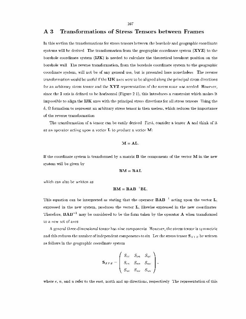
A Transformations of Stress Tensors between Frames
In this section the transformations for stress tensors between the borehole and geographic coordinate
systems will be derived The transformation from the geographic coordinate system XYZ to the
borehole coordinate system IJK is needed to calculate the theoretical breakout position on the
borehole wall The reverse transformation from the borehole coordinate system to the geographic
coordinate system will not be of any general use but is presented here nonetheless The reverse
transformation would be useful if the IJK axes were to be aligned along the principal stress directions
for an arbitrary stress tensor and the XYZ representation of the stress state was needed However
since the I axis is dened to be horizontal Figure this introduces a constraint which makes it
impossible to align the IJK axes with the principal stress directions for all stress tensors Using the
formalism to represent an arbitrary stress tensor is then useless which reduces the importance
of the reverse transformation
The transformation of a tensor can be easily derived First consider a tensor A and think of it
as an operator acting upon a vector L to produce a vectorM
M AL
If the coordinate system is transformed by a matrix B the components of the vectorM in the new
system will be given by
BM BAL
which can also be written as
BM BABBL
This equation can be interpreted as stating that the operator BAB acting upon the vector L
expressed in the new system produces the vector L likewise expressed in the new coordinates
Therefore BAB may be considered to be the form taken by the operator A when transformed
to a new set of axes
A general threedimensional tensor has nine components However the stress tensor is symmetric
and this reduces the number of independent components to six Let the stress tensor SXY Z be written
as follows in the geographic coordinate system
SXY Z
BBB
See Sen Sue
Sen Snn Snu
Sue Snu Suu
CCCA
where e n and u refer to the east north and up directions respectively The representation of this

tensor in the borehole coordinate system is obtained by applying the above transformation
SIJK RSXY ZRT
BBB
cos sin
sin cos cos cos sin
sin sin cos sin cos
CCCASXY Z
BBB
cos sin cos sin sin
sin cos cos cos sin
sin cos
CCCA
BBB
Sii Sij Ski
Sij Sjj Sjk
Ski Sjk Skk
CCCA
The simplied individual components are
Sii See cos Sen sin Snn sin
Sjj Snn cos Sen sin See sin
cos Suu sin Snu cos Sue sin sin
Skk Snn cos Sen sin See sin
sin Suu cos Snu cos Sue sin sin
Sij Sen cos
See Snn sin cos Sue cos Snu sin sin
Sjk Snu cos Sue sin cos
Suu Snn cos
See sin Sen sin sin
Ski Sue cos Snu sin cos Sen cos sin
Snn See sin sin
To nd the reverse transformation start with the following stress tensor in the borehole coordi
nate system
SIJK
BBB
Sii Sij Ski
Sij Sjj Sjk
Ski Sjk Skk
CCCA
To represent SIJK in the geographic coordinate system apply the transformation
SXY Z RTSIJKR
The individual components of SXY Z are
See Sii cos sinSij cos Ski sin sin
Sjj cos Sjk sin Skk sin
Snn Sii sin sin Sij cos Ski sin cos
Sjj cos Sjk sin Skk sin
Suu Sjj sin Sjk sin Skk cos
Sen cos Sij cos Ski sin
sin Sjj cos
Skk sin Sjk sin Sii
Snu Sjk cos cos sin Ski cos Sij sin
cos sin Sjj Skk

Sue Sjk sin cos cos Ski cos Sij sin
sin sin Sjj Skk
A Transforming Angles between the Borehole and Geo
graphic Coordinate Systems
In the previous section the rotation matrices for converting the representation of vectors and tensors
between the borehole and geographic coordinate systems were found These matrices will be used
to describe how the angles measured in one coordinate system translate to angles in the other
coordinate system
The following derivations transform geographic azimuths to angles measured counterclockwise
from the I axis and back I have chosen not to dene an azimuth for the borehole coordinate
system since north is not a natural direction in the IJK coordinate system
Angles are transformed by rst constructing a vector in the appropriate coordinate system that
points in the direction of the angle The rotation matrix R or the inverse rotation matrix RT is
then used to represent the vector in the other coordinate system The vector is then projected onto
either the XY or IJ plane Finally the angle between the projected vector and a coordinate system
axis is calculated
An ambiguity arises in projecting the vector to either theXY or IJ plane Two natural directions
exist in the system the Z and K directions In one case some multiple of Z axis can be added to
the vector to remove its out of the plane component In the other case a multiple of the K axis can
be used Both methods are equally valid but the choice of the proper projection depends upon the
use of the transformed angle
Throughout this work the Z vector will be used to remove the outoftheplane component of
transformed vectors following the usage of Mastin More importantly use of the K vector
fails for horizontal boreholes For this reason the rst method will be used to present results and
calculations However for completeness sake the borehole axis projections may prove useful and
so will be calculated
For example the relative bearing is measured in the borehole coordinate system and the vector
representing this angle would be constructed in the IJK coordinate system This vector would then
be transformed into the XYZ frame using RT Finally the Z component of the transformed vector
would be removed either by just setting it to zero which implicitly implies a projection along the Z
axis or subtracting a multiple of KXY Z

A Using Vertical Projections to Convert a Borehole Angle into a
Geographic Azimuth
Dene the angle as measured from the I axis towards the J axis as a Then the vector representing
this angle is
VIJK
BBBcosa
sina
CCCA
Multiply VIJK by RT to nd the vector as expressed in the geographic reference frame
VXY Z
BBB
cos sin cos sin sin
sin cos cos cos sin
sin cos
CCCA
BBBcosa
sina
CCCA
BBB
cos cosa sin cos sina
sin cosa cos cos sina
sin sina
CCCA
A vector parallel to the Z axis will be used to project VXY Z to the horizontal However the x and
y components of VXY Z will remain unchanged by the addition of a vector parallel to Z The arctan
then is used to nd the azimuth that VXY Z makes with geographic north
tanVXY ZxVXY Zy
tancos cosa sin cos sina
sin cosa cos cos sina
A Using Vertical Projections to Convert a Geographic Azimuth into
a Borehole Angle
The vector representing the geographic azimuth is written as
VXY Z
BBBsin
cos
CCCA
The representation of VXY Z in the IJK reference frame is found using the rotation matrix R
VIJK
BBB
cos sin
sin cos cos cos sin
sin sin cos sin cos
CCCA
BBBsin
cos
CCCA

BBB
cos sin sin cos
sin cos sin cos cos cos
sin sin sin cos sin cos
CCCA
The k component of VIJK is brought to zero by subtracting a vector parallel to Z of suitable length
To do this it is rst necessary to express the Z axis in the IJK frame
ZIJK
BBB
cos sin
sin cos cos cos sin
sin sin cos sin cos
CCCA
BBB
CCCA
BBB
sin
cos
CCCA
Let b be the multiple of ZIJK such that
VIJKk bZIJKk
Then
sin sin sin cos sin cos b cos
b tan cos
The projected vector is
FIJK VIJK bZIJK
BBB
cos sin sin cos
sin cos sin cos cos cos
sin sin sin cos sin cos
CCCA tan cos
BBB
sin
cos
CCCA
BBB
sin
sec cos
CCCA
The resulting angle is
a tanFIJKyFIJKx
tansec cos
sin

A Using Borehole Projections to Convert a Borehole Angle into a
Geographic Azimuth
Dene a as the angle as measured from the I axis towards the J axis Then the vector representing
this angle is
VIJK
BBBcosa
sina
CCCA
Multiply VIJK with RT to nd the vector as expressed in the geographic reference frame
VXY Z
BBB
cos sin cos sin sin
sin cos cos cos sin
sin cos
CCCA
BBBcosa
sina
CCCA
BBB
cos cosa sin cos sina
sin cosa cos cos sina
sin sina
CCCA
Remove the z component of VXY Z by subtracting a vector parallel to K of suitable length Find
the representation of K in the geographic reference frame
KXY Z
BBB
cos sin cos sin sin
sin cos cos cos sin
sin cos
CCCA
BBB
CCCA
BBB sin sin
cos sin
cos
CCCA
Find b such that
VXY Zz bKXY Zz
Then
sin sina b cos
b sina tan
So the resulting vector which lies in the horizontal plane is
FXY Z VXY Z bKXY Z

BBB
cos cosa sin cos sina sina tan sin sin
sin cosa cos cos sina sina tan cos sin
CCCA
and the geographic azimuth is the arc tangent of the x component of the above vector divided
by its y component
tanFXY ZxFXY Zy
tancos cosa sin cos sina sina tan sin sin
sin cosa cos cos sina sina tan cos sin
A Using Borehole Projections to Convert a Geographic Azimuth into
a Borehole Angle
The vector representing the geographic azimuth is written as
VXY Z
BBBsin
cos
CCCA
This is rotated into the borehole reference frame with the rotation matrix R
VIJK
BBB
cos sin
sin cos cos cos sin
sin sin cos sin cos
CCCA
BBBsin
cos
CCCA
BBB
cos sin sin cos
sin cos sin cos cos cos
sin sin sin cos sin cos
CCCA
BBB
sin
cos cos
cos sin
CCCA
The vector addition of a suitable parallel to K vector to VIJK will result in a vector with a k
component This addition will not a ect the i and j component of VIJK so the angle a can be
quickly determined to be
a tanVIJKjVIJKi
tancos cos
sin
Appendix B Cook Inlet Individual Discussion of
Wells
This appendix presents discussion of the important notes problems or inconsistent breakout orien
tations from each Cook Inlet well No stress state inversions were done using the breakouts identied
from an individual well since the number of breakouts was small or occupied a limited area of the
borehole orientation space as seen on lower hemisphere stereograph projection plots
B Gprd
Five di erent sections of digital dipmeter data along with the directional survey and marker data
were received from Unocal The maximum hole deviation in the digital dipmeter data is The ve
di erent sections of hole span the log depth ranges m le m le
m le m le and m le The le refers to the le
number of the digital dipmeter Unocal sent The depth range of the data from le completely
overlaps the depth range of the data in le Since only one log is needed to cover the same depth
interval and since le covers a larger depth range than le le was not used
This hole has relatively constant tool orientations throughout most of the hole according to the
long stretches of almost constant pad azimuth Figure B The caliper arm data is fairly well
behaved with several sections of washedout hole and sections of ingauge hole longer than m
totaling m in length
Out of the m of logged hole m of borehole breakouts were identied All of the
breakouts found are shown in Figure B The two dipmeter runs le and le that covered
the same interval of hole from to m did not have any identied breakouts Since all of
the nonradial breakouts occur in the same m interval from to m no separate plots
of the breakouts as a function of depth are shown
Breakouts were found in the following markers TSS breakouts for m BSS
breakout for m TM breakout for m TSS breakout for m BSS
breakout for m BSS breakout for m TM breakouts for m TM
breakouts for m TMX breakouts for m TM breakout for m TMX breakout
for m TXSSA breakout for m BXSSA breakouts for m and TM
breakouts for m Breakouts may lie in more than one marker which accounts for those markers
that list breakouts shorter than the minimum breakout length of m

At shallower depths the breakout pattern varies smoothly as a function of depth At m
TVD the breakouts are oriented NE and slowly rotate to NE at m TVD Eight
meters lower is another breakout oriented NE an counterclockwise orientation change
From this point on the breakouts continue to vary slowly to NW The sharp transition occurs
where the m wide TXSSA marker is bounded by TMX on top and by the BXSSA
marker on the bottom While no information about the material properties or about the dips of
the formations near this transition were received from Unocal it is possible that material property
or bedding dip di erences between the two markers caused this large transition The marker le
does not indicate that any faults were crossed by this well Only one breakout was identied in the
TXSS marker Figure B

10
20
30
40
50
60
Cal
iper
Arm
s (c
entim
eter
s)
2200 2400 2600 2800 3000 3200 3400 3600
Log Depth (meters)
0
Cal
iper
Arm
s (c
entim
eter
s)
0
Log Depth (meters)
10
20
30
40
50
60
2200 2400 2600 2800 3000 3200 3400 3600
00
10
20
30
40
50
60
2200 2400 2600 2800 3000 3200 3400 3600
00
10
20
30
40
50
60
2200 2400 2600 2800 3000 3200 3400 3600
00
10
20
30
40
50
60
2200 2400 2600 2800 3000 3200 3400 3600
00
10
20
30
40
50
60
2200 2400 2600 2800 3000 3200 3400 3600
00
10
20
30
40
50
60
2200 2400 2600 2800 3000 3200 3400 3600
00
10
20
30
40
50
60
2200 2400 2600 2800 3000 3200 3400 3600
00
10
20
30
40
50
60
2200 2400 2600 2800 3000 3200 3400 3600
00
10
20
30
40
50
60
2200 2400 2600 2800 3000 3200 3400 3600
00
10
20
30
40
50
60
2200 2400 2600 2800 3000 3200 3400 3600
00
10
20
30
40
50
60
2200 2400 2600 2800 3000 3200 3400 3600
00
10
20
30
40
50
60
2200 2400 2600 2800 3000 3200 3400 3600
00
5
10
15
20
Dev
iatio
n (d
egre
es)
2200 2400 2600 2800 3000 3200 3400 3600
Tm29
Tm30
Tm31
Tm32
Tm33
Tm34
Tm35
Tm36
Tm37
Tm38
Tm39
T3940ss
B3940ss
Tm40
T4041ss
B4041ss
Tm41
T4142ss
B4142ss
Tm42
T4243ss
B4243ss
Tm43
T4344ss
B4344ss
Tm44
Tm45
T45xss
B45xss
Tm46
Tmx
T46xssa47
B46xssa47
Tm47
Tm48
Tm49
Tm52
Tm53
Them
Twf
Frlog
Dtdt
0
Dev
iatio
n (d
egre
es)
0
5
10
15
20
2200 2400 2600 2800 3000 3200 3400 3600
00
5
10
15
20
2200 2400 2600 2800 3000 3200 3400 3600
00
5
10
15
20
2200 2400 2600 2800 3000 3200 3400 3600
00
5
10
15
20
2200 2400 2600 2800 3000 3200 3400 3600
00
0
100
200
300
400
Azi
mut
hs (
degr
ees)
2200 2400 2600 2800 3000 3200 3400 3600
0
Azi
mut
hs (
degr
ees)
0
0
100
200
300
400
2200 2400 2600 2800 3000 3200 3400 3600
00
0
100
200
300
400
2200 2400 2600 2800 3000 3200 3400 3600
00
0
100
200
300
400
2200 2400 2600 2800 3000 3200 3400 3600
00
0
100
200
300
400
2200 2400 2600 2800 3000 3200 3400 3600
00
0
100
200
300
400
2200 2400 2600 2800 3000 3200 3400 3600
00
0
100
200
300
400
2200 2400 2600 2800 3000 3200 3400 3600
00
0
100
200
300
400
2200 2400 2600 2800 3000 3200 3400 3600
00
0
100
200
300
400
2200 2400 2600 2800 3000 3200 3400 3600
00
0
100
200
300
400
2200 2400 2600 2800 3000 3200 3400 3600
00
0
100
200
300
400
2200 2400 2600 2800 3000 3200 3400 3600
00
0
100
200
300
400
2200 2400 2600 2800 3000 3200 3400 3600
00
0
100
200
300
400
2200 2400 2600 2800 3000 3200 3400 3600
00
Figure B Plots of the calipercalibrated and declinationcorrected digitized dipmeter and derivedquantities data as a function of well depth from well Gprd top Borehole elongation directionsolid line pad azimuth dotted line and borehole azimuth dashed line middle Boreholedeviation solid curve and location of marker horizons vertical lines with labels bottom Bit sizestraight solid line caliper arm solid line and caliper arm dotted line Selected breakoutregions are plotted as horizontal bars showing the depth extent of the breakouts

N
S
EW
9.0
18.0
27.0
36.0
45.0
54.0-2928.2
-2422.5N
S
EW
9.0
18.0
27.0
36.0
45.0
54.0-2928.2
-2645.6
Figure B Lower hemisphere stereographic projection plots of the selected breakouts from wellGprd Line widths are proportional to the breakout length left All selected breakoutsright All nonradial breakouts where the IJK breakout angle is not within of the high side ofthe hole
N
S
EW
9.0
18.0
27.0
36.0
45.0
54.0-2678.8
-2678.8N
S
EW
9.0
18.0
27.0
36.0
45.0
54.0-2678.8
-2678.8
Figure B Lower hemisphere stereographic projection plots of the selected breakouts from wellGprd in marker TXSS Line widths are proportional to the breakout length left Allselected breakouts in TXSS right All nonradial breakouts in TXSS where the IJK breakoutangle is not within of the high side of the hole

B Gprd
Five di erent digitally logged sections of Gprd were received The ve di erent sections span
the log depth ranges m le m le m le
m le m le The depth range of the data from le almost completely
overlaps the depth range of the data in le Since only one well log is needed to cover the same
depth interval and since le covers a larger depth range than le le was not used in any
breakout calculations No breakouts were found in either le in the overlapping interval File
and also partially overlap each other File had two breakouts the rst at m log depth
which was not found in the other well log and the second at depth m was on the boundary
of where le ends File also has two breakouts which are just above the shallowest logged depth
in le Since there are no consistent breakouts found in both logs and one breakout is found in
only one hole le was used since it has two breakouts that are not in conict with the other le
The maximum deviation throughout these sections is while the maximum deviation of the
hole is The dipmeter tool had a tendency to rotate when it logged ingauge sections of the
hole Figures B Ingauge sections of the hole longer than m accounted for m of the
dipmeter data with an average length of m
The breakout selection scheme identied m of breakouts averaging m in length All of
the borehole breakouts are plotted in Figure B and the nonradial breakouts separated into m
TVD intervals are plotted in Figure B No breakouts were found in the TXSS marker The
breakouts were observed in the TSS breakouts for m the BSS breakout for m
and the TXSSA breakouts for m markers
The breakouts are observed over a m TVD interval from m to m The break
out orientations range from ESEWNW to NENW However as the borehole orientation moves
from a WSW trend to a SE trend the breakouts orientations decrease from NE to NE
and than increase to NE Since the breakouts from Gprd do not cover a large amount of
borehole orientation space in the lower hemisphere stereograph projection plots doing a numerical
inversion of the data would not prove useful It does not appear that any simple stress state would
explain the breakout pattern due to the inconsistency of breakout rotations as a function of depth
However the two deepest breakouts that are rotated clockwise with respect to the breakouts above
them were found to be in the TXSSA marker the same marker where an counterclockwise
rotation was observed in Gprds breakout orientations The TXSSA could have substan
tially di erent bedding dips or material properties to a ect the stress state and hence the observed
breakouts

10
20
30
40
50
60
Cal
iper
Arm
s (c
entim
eter
s)
2400 2500 2600 2700 2800 2900 3000 3100
Log Depth (meters)
0
Cal
iper
Arm
s (c
entim
eter
s)
0
Log Depth (meters)
10
20
30
40
50
60
2400 2500 2600 2700 2800 2900 3000 3100
00
10
20
30
40
50
60
2400 2500 2600 2700 2800 2900 3000 3100
00
10
20
30
40
50
60
2400 2500 2600 2700 2800 2900 3000 3100
00
10
20
30
40
50
60
2400 2500 2600 2700 2800 2900 3000 3100
00
10
20
30
40
50
60
2400 2500 2600 2700 2800 2900 3000 3100
00
10
20
30
40
50
60
2400 2500 2600 2700 2800 2900 3000 3100
00
10
20
30
40
50
60
2400 2500 2600 2700 2800 2900 3000 3100
00
10
20
30
40
50
60
2400 2500 2600 2700 2800 2900 3000 3100
00
10
20
30
40
50
60
2400 2500 2600 2700 2800 2900 3000 3100
00
2
4
6
8
10
12
14
16
18
Dev
iatio
n (d
egre
es)
2400 2500 2600 2700 2800 2900 3000 3100
Lrlog
Kop
B3940ss
Tm40
Tm41
T4142ss
B4142ss
Tm42a
T4243ss
B4243ss
Tm43
Tm44
T4445ss
B4445ss
Tm45
T45xss
T45cq
B45xss
Tmx
T46xssa47
B46xssa47
Frlog
0
Dev
iatio
n (d
egre
es)
0
2
4
6
8
10
12
14
16
18
2400 2500 2600 2700 2800 2900 3000 3100
00
2
4
6
8
10
12
14
16
18
2400 2500 2600 2700 2800 2900 3000 3100
00
2
4
6
8
10
12
14
16
18
2400 2500 2600 2700 2800 2900 3000 3100
00
0
100
200
300
400
Azi
mut
hs (
degr
ees)
2400 2500 2600 2700 2800 2900 3000 3100
0
Azi
mut
hs (
degr
ees)
0
0
100
200
300
400
2400 2500 2600 2700 2800 2900 3000 3100
00
0
100
200
300
400
2400 2500 2600 2700 2800 2900 3000 3100
00
0
100
200
300
400
2400 2500 2600 2700 2800 2900 3000 3100
00
0
100
200
300
400
2400 2500 2600 2700 2800 2900 3000 3100
00
0
100
200
300
400
2400 2500 2600 2700 2800 2900 3000 3100
00
0
100
200
300
400
2400 2500 2600 2700 2800 2900 3000 3100
00
0
100
200
300
400
2400 2500 2600 2700 2800 2900 3000 3100
00
0
100
200
300
400
2400 2500 2600 2700 2800 2900 3000 3100
00
0
100
200
300
400
2400 2500 2600 2700 2800 2900 3000 3100
00
Figure B Plots of the calipercalibrated and declinationcorrected digitized dipmeter and derivedquantities data as a function of well depth from well Gprd top Borehole elongation directionsolid line pad azimuth dotted line and borehole azimuth dashed line middle Boreholedeviation solid curve and location of marker horizons vertical lines with labels bottom Bit sizestraight solid line caliper arm solid line and caliper arm dotted line Selected breakoutregions are plotted as horizontal bars showing the depth extent of the breakouts

N
S
EW
9.0
18.0
27.0
36.0
45.0
54.0-2795.5
-2308.4N
S
EW
9.0
18.0
27.0
36.0
45.0
54.0-2795.5
-2308.4
Figure B Lower hemisphere stereographic projection plots of the selected breakouts from wellGprd Line widths are proportional to the breakout length left All selected breakouts rightAll nonradial breakouts where the IJK breakout angle is not within of the high side of the hole
N
S
EW
9.0
18.0
27.0
36.0
45.0
54.0-2308.4
-2308.4N
S
EW
9.0
18.0
27.0
36.0
45.0
54.0-2795.5
-2786.5
Figure B Lower hemisphere stereographic projection plots of all nonradial breakouts from wellGprd between the true vertical depths of m on the left and m on the right

B Gprd
The digital dipmeter data for Granite Point rd came as three separate data les spanning the log
depth ranges m le m le m le The raw digital
dipmeter data along with the calculated borehole elongation directions are shown in and combined
in Figure B Over half of the logged interval has one caliper arm ingauge with the other caliper
arm broken out In only m or of the logged interval were both caliper arms ingauge
over a m interval No substantial tool rotation occurred in these intervals probably due to the
short m average length of the ingauge sections
The breakout selection scheme identied breakouts having a combined length of m The
deeper section of hole below roughly m log depth is much more consistent and ingauge than
the upper section of hole However the shallower section had all but two of the identied breakouts
The shallower section is identied by one caliper arm consistently being ingauge while the other
caliper arm is consistently at least cm out of gauge Only in those sections where the larger caliper
arm showed enough caliper arm length consistently were breakouts identied
Breakouts were identied in the following markers TM breakouts for m TM
breakout for m TM breakout for m TM breakouts for m TM breakout
for m TM breakout for m TM breakout for m and TSS breakout for
m
Granite Point rd breakouts have a consistent breakout orientation of roughly NE regardless
of the borehole azimuth which is varies from SW to SW and the borehole deviation which
varies from to Figure B Since the breakout orientations are so constant any stress
state nodal points would not plot near the measured data on the lower hemisphere stereographic
projection plot Since all of the nonradial breakouts occur in the to m depth interval
the breakouts are not plotted separately in m intervals Also no breakouts were found in the
TXSS marker

10
20
30
40
50
Cal
iper
Arm
s (c
entim
eter
s)
2000 2200 2400 2600 2800 3000 3200
Log Depth (meters)
0
Cal
iper
Arm
s (c
entim
eter
s)
0
Log Depth (meters)
10
20
30
40
50
2000 2200 2400 2600 2800 3000 3200
00
10
20
30
40
50
2000 2200 2400 2600 2800 3000 3200
00
10
20
30
40
50
2000 2200 2400 2600 2800 3000 3200
00
10
20
30
40
50
2000 2200 2400 2600 2800 3000 3200
00
10
20
30
40
50
2000 2200 2400 2600 2800 3000 3200
00
10
20
30
40
50
2000 2200 2400 2600 2800 3000 3200
00
10
20
30
40
50
2000 2200 2400 2600 2800 3000 3200
00
10
20
30
40
50
2000 2200 2400 2600 2800 3000 3200
00
10
20
30
40
50
2000 2200 2400 2600 2800 3000 3200
00
10
20
30
40
50
Dev
iatio
n (d
egre
es)
2000 2200 2400 2600 2800 3000 3200
Lrlog
Tm26
Tm27
Tm28
Tm29
Tm30
Tm31
Tm32
Tm34
Tm35
Tm39a
T3940ss
B3940ss
Tm40
T4040ass
B4040ass
Tm40a
Tm40b
T40a41ass
B40a41ass
Tm41a
Tm41b
Tm42a
T4243ss
B4243ss
Tm43
Tm44
T4445ss
B4445ss
T45xss
Tm45c
B45xss
Tmx
T46xssa47
B46xssa47
Tm47
Tm48
T4849ss
Frlog
0
Dev
iatio
n (d
egre
es)
0
10
20
30
40
50
2000 2200 2400 2600 2800 3000 3200
00
10
20
30
40
50
2000 2200 2400 2600 2800 3000 3200
00
10
20
30
40
50
2000 2200 2400 2600 2800 3000 3200
00
0
50
100
150
200
250
300
350
Azi
mut
hs (
degr
ees)
2000 2200 2400 2600 2800 3000 3200
0
Azi
mut
hs (
degr
ees)
0
0
50
100
150
200
250
300
350
2000 2200 2400 2600 2800 3000 3200
00
0
50
100
150
200
250
300
350
2000 2200 2400 2600 2800 3000 3200
00
0
50
100
150
200
250
300
350
2000 2200 2400 2600 2800 3000 3200
00
0
50
100
150
200
250
300
350
2000 2200 2400 2600 2800 3000 3200
00
0
50
100
150
200
250
300
350
2000 2200 2400 2600 2800 3000 3200
00
0
50
100
150
200
250
300
350
2000 2200 2400 2600 2800 3000 3200
00
0
50
100
150
200
250
300
350
2000 2200 2400 2600 2800 3000 3200
00
0
50
100
150
200
250
300
350
2000 2200 2400 2600 2800 3000 3200
00
0
50
100
150
200
250
300
350
2000 2200 2400 2600 2800 3000 3200
00
Figure B Plots of the calipercalibrated and declinationcorrected digitized dipmeter and derivedquantities data as a function of well depth from well Gprd top Borehole elongation directionsolid line pad azimuth dotted line and borehole azimuth dashed line middle Boreholedeviation solid curve and location of marker horizons vertical lines with labels bottom Bit sizestraight solid line caliper arm solid line and caliper arm dotted line Selected breakoutregions are plotted as horizontal bars showing the depth extent of the breakouts

N
S
EW
9.0
18.0
27.0
36.0
45.0
54.0-2695.7
-2150.1N
S
EW
9.0
18.0
27.0
36.0
45.0
54.0-2281.5
-2150.1
Figure B Lower hemisphere stereographic projection plots of the selected breakouts from wellGprd Line widths are proportional to the breakout length left All selected breakouts rightAll nonradial breakouts where the IJK breakout angle is not within of the high side of the hole

B Gprd
Two digital dipmeter les le and le were received for Granite Point rd The top of both
logged sections begin at m log depth File which stops at m log depth is the shorter
of the two sections le stops at m Both dipmeter runs have the same character caliper arm
and pad azimuth data Figures B and B The dipmeter did not rotate throughout either
logging run due to a sizeable di erence between the two caliper arm diameters No tool rotation
occurred in the di erent ingauge sections of hole longer than m which amounted to m
of the dipmeter data
The depth range m was logged with both dipmeter runs and over this depth interval
both dipmeter runs had identied breakouts The breakouts from each hole had similar depths
lengths and most importantly IJK breakout angle the angle between the high side of the hole and
the breakout as measured in the plane perpendicular to the borehole axis Table B lists the log
depth the breakout length the XYZ breakout azimuth and the IJK breakout angle The largest
di erence between the measured IJK breakout angles for similarly measured breakouts is for
the second shallowest breakout While the IJK breakout angles are very consistent between the two
dipmeter runs the total length of breakouts identied di ers by m which is large given that the
two dipmeters logged only m of common hole This di erence could be due to the two separate
logging runs where the tool drag from the rst gauged out the bottom of the hole enough for the
second run to identify more breakouts Since the le dipmeter log is longer the remaining analysis
of the breakout data was done using le
Plotting the breakout azimuths on a lower hemisphere stereographic projection plot shows that
all of the breakouts are aligned with the high and low sides of the borehole Figure B This
observation combined with the observation of no pad rotation in the top plot of Figure B suggests
that the dipmeter was tracking only the high and low side of the hole and that these breakouts are
questionable Most of the stress state analyses done later in this chapter use nonradial breakouts
and so the data from this borehole will be discarded Even though the breakouts are questionable
it is an encouraging sign to have two dipmeter runs identify breakouts in same positions of the
borehole
None of the identied breakouts were found in the TXSS marker Breakouts were identied in
the TMAEST breakouts for m TSS breakouts for m BSS breakout
for m TM breakouts for m TASS breakout for m BASS breakout
for m TMA breakout for m BAASS breakout for m TAASS
breakout for m TMA breakout for m and the TAASS breakouts for m
markers

10
15
20
25
30
35
Cal
iper
Arm
s (c
entim
eter
s)
3080 3100 3120 3140 3160 3180 3200 3220 3240 3260 3280
Log Depth (meters)
0
Cal
iper
Arm
s (c
entim
eter
s)
0
Log Depth (meters)
10
15
20
25
30
35
3080 3100 3120 3140 3160 3180 3200 3220 3240 3260 3280
00
10
15
20
25
30
35
3080 3100 3120 3140 3160 3180 3200 3220 3240 3260 3280
00
10
15
20
25
30
35
3080 3100 3120 3140 3160 3180 3200 3220 3240 3260 3280
00
22.8
22.9
23.0
23.1
23.2
23.3
23.4
23.5
Dev
iatio
n (d
egre
es)
3080 3100 3120 3140 3160 3180 3200 3220 3240 3260 3280
Tm37
Tm39aest
T3940ss
B3940ss
Tm40
T4040ass
B4040ass
Tm40a
T40a41ass
B40a41ass
Tm41a
T41a42ass
B41a42ass
Tm42a
0.00.10.20.30.40.50.60.70.80.91.0
Dev
iatio
n (d
egre
es)
0
22.8
22.9
23.0
23.1
23.2
23.3
23.4
23.5
3080 3100 3120 3140 3160 3180 3200 3220 3240 3260 3280
0.00.10.20.30.40.50.60.70.80.91.00
0
100
200
300
400
Azi
mut
hs (
degr
ees)
3080 3100 3120 3140 3160 3180 3200 3220 3240 3260 3280
0
Azi
mut
hs (
degr
ees)
0
0
100
200
300
400
3080 3100 3120 3140 3160 3180 3200 3220 3240 3260 3280
00
0
100
200
300
400
3080 3100 3120 3140 3160 3180 3200 3220 3240 3260 3280
00
0
100
200
300
400
3080 3100 3120 3140 3160 3180 3200 3220 3240 3260 3280
00
Figure B Plots of the calipercalibrated and declinationcorrected digitized dipmeter and derivedquantities data as a function of well depth from well Gprd le top Borehole elongationdirection solid line pad azimuth dotted line and borehole azimuth dashed line middleBorehole deviation solid curve and location of marker horizons vertical lines with labels bottomBit size straight solid line caliper arm solid line and caliper arm dotted line Selectedbreakout regions are plotted as horizontal bars showing the depth extent of the breakouts

20
22
24
26
28
30
32
34
Cal
iper
Arm
s (c
entim
eter
s)
3090 3100 3110 3120 3130 3140 3150 3160 3170
Log Depth (meters)
0
Cal
iper
Arm
s (c
entim
eter
s)
0
Log Depth (meters)
20
22
24
26
28
30
32
34
3090 3100 3110 3120 3130 3140 3150 3160 3170
00
20
22
24
26
28
30
32
34
3090 3100 3110 3120 3130 3140 3150 3160 3170
00
20
22
24
26
28
30
32
34
3090 3100 3110 3120 3130 3140 3150 3160 3170
00
23.10
23.15
23.20
23.25
23.30
23.35
23.40
Dev
iatio
n (d
egre
es)
3090 3100 3110 3120 3130 3140 3150 3160 3170
Tm37
Tm39aest
T3940ss
B3940ss
Tm40
T4040ass
B4040ass
Tm40a
0.000.050.100.150.200.250.300.350.400.450.500.550.600.650.700.750.800.850.900.951.00
Dev
iatio
n (d
egre
es)
0
23.10
23.15
23.20
23.25
23.30
23.35
23.40
3090 3100 3110 3120 3130 3140 3150 3160 3170
0.000.050.100.150.200.250.300.350.400.450.500.550.600.650.700.750.800.850.900.951.000
0
50
100
150
200
250
Azi
mut
hs (
degr
ees)
3090 3100 3110 3120 3130 3140 3150 3160 3170
0
Azi
mut
hs (
degr
ees)
0
0
50
100
150
200
250
3090 3100 3110 3120 3130 3140 3150 3160 3170
00
0
50
100
150
200
250
3090 3100 3110 3120 3130 3140 3150 3160 3170
00
0
50
100
150
200
250
3090 3100 3110 3120 3130 3140 3150 3160 3170
00
Figure B Plots of the calipercalibrated and declinationcorrected digitized dipmeter and derivedquantities data as a function of well depth from well Gprd le top Borehole elongationdirection solid line pad azimuth dotted line and borehole azimuth dashed line middleBorehole deviation solid curve and location of marker horizons vertical lines with labels bottomBit size straight solid line caliper arm solid line and caliper arm dotted line Selectedbreakout regions are plotted as horizontal bars showing the depth extent of the breakouts

N
S
EW
9.0
18.0
27.0
36.0
45.0
54.0-2764.1
-2625N
S
EW
9.0
18.0
27.0
36.0
45.0
54.0
Figure B Lower hemisphere stereographic projection plots of the selected breakouts from wellGprd Line widths are proportional to the breakout length left All selected breakouts rightAll nonradial breakouts where the IJK breakout angle is not within of the high side of the hole
Table B List of the breakouts identied in two separate dipmeter runs over the to mlog foot depth interval in Gprd with le on the left and le on the right The identied IJKbreakout angle results from the two log les agree within
Gprd le Gprd le XYZ IJK XYZ IJK
Log Breakout Breakout Log Breakout Breakoutdepth Length Azimuth Angle depth Length Azimuth Anglem m m m
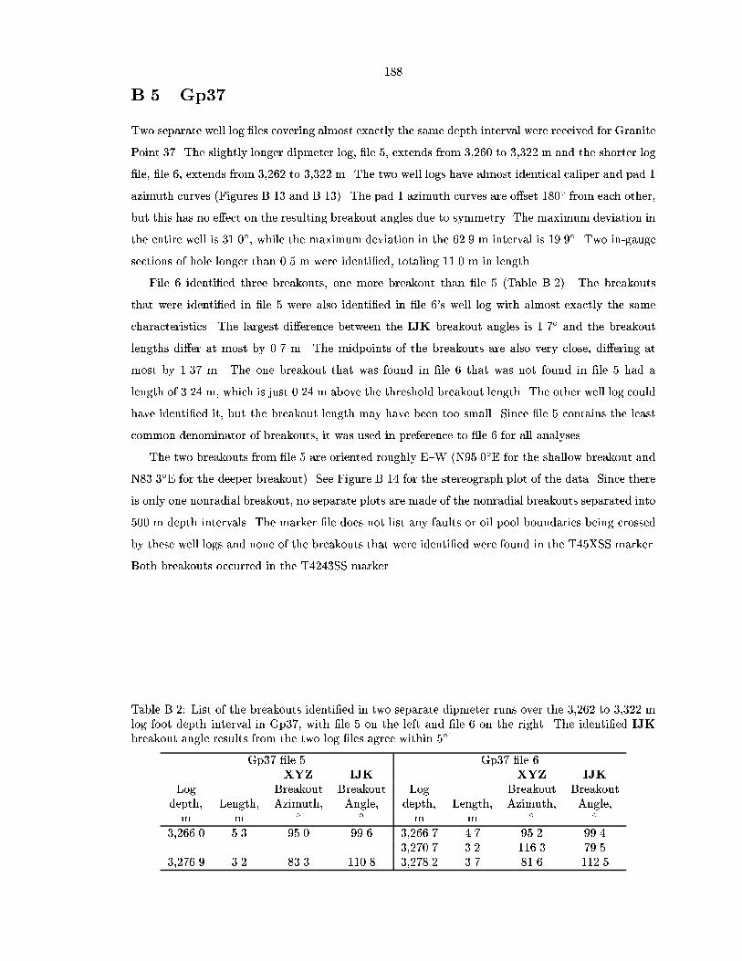
B Gp
Two separate well log les covering almost exactly the same depth interval were received for Granite
Point The slightly longer dipmeter log le extends from to m and the shorter log
le le extends from to m The two well logs have almost identical caliper and pad
azimuth curves Figures B and B The pad azimuth curves are o set from each other
but this has no e ect on the resulting breakout angles due to symmetry The maximum deviation in
the entire well is while the maximum deviation in the m interval is Two ingauge
sections of hole longer than m were identied totaling m in length
File identied three breakouts one more breakout than le Table B The breakouts
that were identied in le were also identied in le s well log with almost exactly the same
characteristics The largest di erence between the IJK breakout angles is and the breakout
lengths di er at most by m The midpoints of the breakouts are also very close di ering at
most by m The one breakout that was found in le that was not found in le had a
length of m which is just m above the threshold breakout length The other well log could
have identied it but the breakout length may have been too small Since le contains the least
common denominator of breakouts it was used in preference to le for all analyses
The two breakouts from le are oriented roughly EW NE for the shallow breakout and
NE for the deeper breakout See Figure B for the stereograph plot of the data Since there
is only one nonradial breakout no separate plots are made of the nonradial breakouts separated into
m depth intervals The marker le does not list any faults or oil pool boundaries being crossed
by these well logs and none of the breakouts that were identied were found in the TXSS marker
Both breakouts occurred in the TSS marker
Table B List of the breakouts identied in two separate dipmeter runs over the to mlog foot depth interval in Gp with le on the left and le on the right The identied IJKbreakout angle results from the two log les agree within
Gp le Gp le XYZ IJK XYZ IJK
Log Breakout Breakout Log Breakout Breakoutdepth Length Azimuth Angle depth Length Azimuth Anglem m m m

15
20
25
30
35
40
Cal
iper
Arm
s (c
entim
eter
s)
3250 3260 3270 3280 3290 3300 3310 3320 3330
Log Depth (meters)
0
Cal
iper
Arm
s (c
entim
eter
s)
0
Log Depth (meters)
15
20
25
30
35
40
3250 3260 3270 3280 3290 3300 3310 3320 3330
00
15
20
25
30
35
40
3250 3260 3270 3280 3290 3300 3310 3320 3330
00
15
20
25
30
35
40
3250 3260 3270 3280 3290 3300 3310 3320 3330
00
19.5
19.6
19.7
19.8
19.9
Dev
iatio
n (d
egre
es)
3250 3260 3270 3280 3290 3300 3310 3320 3330
Lrlog
T4243ss
B4243ss
Tm43
0.00.10.20.30.40.50.60.70.80.91.0
Dev
iatio
n (d
egre
es)
0
19.5
19.6
19.7
19.8
19.9
3250 3260 3270 3280 3290 3300 3310 3320 3330
0.00.10.20.30.40.50.60.70.80.91.00
0
100
200
300
400
Azi
mut
hs (
degr
ees)
3250 3260 3270 3280 3290 3300 3310 3320 3330
0
Azi
mut
hs (
degr
ees)
0
0
100
200
300
400
3250 3260 3270 3280 3290 3300 3310 3320 3330
00
0
100
200
300
400
3250 3260 3270 3280 3290 3300 3310 3320 3330
00
0
100
200
300
400
3250 3260 3270 3280 3290 3300 3310 3320 3330
00
Figure B Plots of the calipercalibrated and declinationcorrected digitized dipmeter and derivedquantities data as a function of well depth from well Gp le top Borehole elongation directionsolid line pad azimuth dotted line and borehole azimuth dashed line middle Boreholedeviation solid curve and location of marker horizons vertical lines with labels bottom Bit sizestraight solid line caliper arm solid line and caliper arm dotted line Selected breakoutregions are plotted as horizontal bars showing the depth extent of the breakouts

15
20
25
30
35
40
Cal
iper
Arm
s (c
entim
eter
s)
3260 3270 3280 3290 3300 3310 3320 3330
Log Depth (meters)
0
Cal
iper
Arm
s (c
entim
eter
s)
0
Log Depth (meters)
15
20
25
30
35
40
3260 3270 3280 3290 3300 3310 3320 3330
00
15
20
25
30
35
40
3260 3270 3280 3290 3300 3310 3320 3330
00
15
20
25
30
35
40
3260 3270 3280 3290 3300 3310 3320 3330
00
19.5
19.6
19.7
19.8
19.9
Dev
iatio
n (d
egre
es)
3260 3270 3280 3290 3300 3310 3320 3330
Lrlog
T4243ss
B4243ss
Tm43
0.00.10.20.30.40.50.60.70.80.91.0
Dev
iatio
n (d
egre
es)
0
19.5
19.6
19.7
19.8
19.9
3260 3270 3280 3290 3300 3310 3320 3330
0.00.10.20.30.40.50.60.70.80.91.00
0
100
200
300
400
Azi
mut
hs (
degr
ees)
3260 3270 3280 3290 3300 3310 3320 3330
0
Azi
mut
hs (
degr
ees)
0
0
100
200
300
400
3260 3270 3280 3290 3300 3310 3320 3330
00
0
100
200
300
400
3260 3270 3280 3290 3300 3310 3320 3330
00
0
100
200
300
400
3260 3270 3280 3290 3300 3310 3320 3330
00
Figure B Plots of the calipercalibrated and declinationcorrected digitized dipmeter and derivedquantities data as a function of well depth from well Gp le top Borehole elongation directionsolid line pad azimuth dotted line and borehole azimuth dashed line middle Boreholedeviation solid curve and location of marker horizons vertical lines with labels bottom Bit sizestraight solid line caliper arm solid line and caliper arm dotted line Selected breakoutregions are plotted as horizontal bars showing the depth extent of the breakouts

N
S
EW
9.0
18.0
27.0
36.0
45.0
54.0-3031.6
-3021.3N
S
EW
9.0
18.0
27.0
36.0
45.0
54.0-3031.6
-3031.6
Figure B Lower hemisphere stereographic projection plots of the selected breakouts from wellGp Line widths are proportional to the breakout length left All selected breakouts right Allnonradial breakouts where the IJK breakout angle is not within of the high side of the hole

B Gp
The digital dipmeter data from Granite Point came as three separate les spanning the log depth
ranges m le m le and m le The maximum
deviation of the hole in these intervals is Since le completely overlaps the same section
of hole logged by le le s data was not used in subsequent calculations The caliper logs has
sections of continuous roughly ingauge sections of hole separated by brokenout and washedout
sections of hole Figure B The ingauge sections have a large amount of tool rotation as shown
by the pad azimuth data There were ingauge sections of hole longer than m totaling
m in length or of the well log data
Only three breakouts all of them in le were identied in this hole because so much of it was
washedout Figure B The three breakouts totaled m in length or of the total length
of dipmeter logs for this hole The deepest identied breakout from le occurs in the depth range
recorded by le However the breakout was not identied in le since the caliper arm data
was much more inconsistent over same the interval where the breakout was identied in le The
three breakouts are oriented fairly consistently at an azimuth of NE Figure B and
the two shallower breakouts occur at the top end of a section of hole where the tool was heavily
rotating No marker les for Granite Point were received Since only one nonradial breakout was
identied no separate plots of nonradial breakouts divided into m intervals are shown
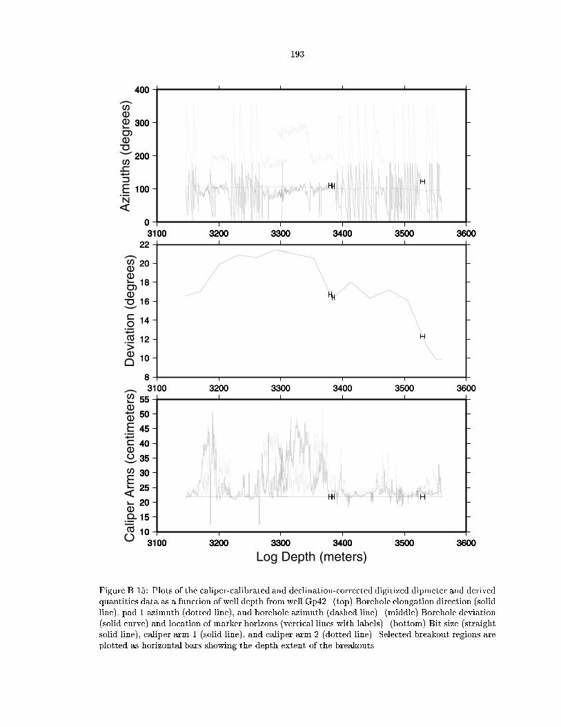
10
15
20
25
30
35
40
45
50
55
Cal
iper
Arm
s (c
entim
eter
s)
3100 3200 3300 3400 3500 3600
Log Depth (meters)
0
Cal
iper
Arm
s (c
entim
eter
s)
0
Log Depth (meters)
10
15
20
25
30
35
40
45
50
55
3100 3200 3300 3400 3500 3600
00
10
15
20
25
30
35
40
45
50
55
3100 3200 3300 3400 3500 3600
00
10
15
20
25
30
35
40
45
50
55
3100 3200 3300 3400 3500 3600
00
10
15
20
25
30
35
40
45
50
55
3100 3200 3300 3400 3500 3600
00
10
15
20
25
30
35
40
45
50
55
3100 3200 3300 3400 3500 3600
00
10
15
20
25
30
35
40
45
50
55
3100 3200 3300 3400 3500 3600
00
8
10
12
14
16
18
20
22
Dev
iatio
n (d
egre
es)
3100 3200 3300 3400 3500 3600
0
Dev
iatio
n (d
egre
es)
0
8
10
12
14
16
18
20
22
3100 3200 3300 3400 3500 3600
00
8
10
12
14
16
18
20
22
3100 3200 3300 3400 3500 3600
00
0
100
200
300
400
Azi
mut
hs (
degr
ees)
3100 3200 3300 3400 3500 3600
0
Azi
mut
hs (
degr
ees)
0
0
100
200
300
400
3100 3200 3300 3400 3500 3600
00
0
100
200
300
400
3100 3200 3300 3400 3500 3600
00
0
100
200
300
400
3100 3200 3300 3400 3500 3600
00
0
100
200
300
400
3100 3200 3300 3400 3500 3600
00
0
100
200
300
400
3100 3200 3300 3400 3500 3600
00
0
100
200
300
400
3100 3200 3300 3400 3500 3600
00
Figure B Plots of the calipercalibrated and declinationcorrected digitized dipmeter and derivedquantities data as a function of well depth from well Gp top Borehole elongation direction solidline pad azimuth dotted line and borehole azimuth dashed line middle Borehole deviationsolid curve and location of marker horizons vertical lines with labels bottom Bit size straightsolid line caliper arm solid line and caliper arm dotted line Selected breakout regions areplotted as horizontal bars showing the depth extent of the breakouts

N
S
EW
9.0
18.0
27.0
36.0
45.0
54.0-2920.6
-2777.8N
S
EW
9.0
18.0
27.0
36.0
45.0
54.0-2920.6
-2920.6
Figure B Lower hemisphere stereographic projection plots of the selected breakouts from wellGp Line widths are proportional to the breakout length left All selected breakouts right Allnonradial breakouts where the IJK breakout angle is not within of the high side of the hole

B Gp
The digital dipmeter data for Granite Point came in two di erent les covering the depth ranges
to m le and to m le log depth The raw dipmeter data are shown
in Figure B The maximum deviation reached in these two sections was The tool has
intermittent rotation throughout the m of log A total m of ingauge hole longer than m
was identied which amounts to of the log
A total of m of breakouts was identied from both dipmeter data sets Figure B which
covers roughly of the well log data The breakouts from le and le have two quite
di erent patterns File s two breakouts are oriented roughly NESE to NNESSW The borehole
elongations from the deeper part of the hole le have a fairly consistent pattern except for the
shallowest breakout Excluding the shallowest breakout which is in the TSS marker the break
out orientations rotate from NE to NE as the borehole azimuth trends from NE to
NE This rotation occurs in the TM TXSS BXSS TM and TMX markers This
well crosses two faults at and m log depth which is deeper than any available well log
data
Since all of the nonradial breakouts are between and m no separate plots of nonradial
breakouts separated into depth zones are shown Instead see Figure B Breakouts were found
in the following markers TM breakout for m BSS breakout for m TM
breakout for m TSS breakout for m TM breakouts for m BXSS
breakouts for m TM breakouts for m and TMX breakouts for m

25
30
35
40
45
50
55
60
Cal
iper
Arm
s (c
entim
eter
s)
2400 2500 2600 2700 2800 2900 3000 3100
Log Depth (meters)
0
Cal
iper
Arm
s (c
entim
eter
s)
0
Log Depth (meters)
25
30
35
40
45
50
55
60
2400 2500 2600 2700 2800 2900 3000 3100
00
25
30
35
40
45
50
55
60
2400 2500 2600 2700 2800 2900 3000 3100
00
25
30
35
40
45
50
55
60
2400 2500 2600 2700 2800 2900 3000 3100
00
25
30
35
40
45
50
55
60
2400 2500 2600 2700 2800 2900 3000 3100
00
25
30
35
40
45
50
55
60
2400 2500 2600 2700 2800 2900 3000 3100
00
25
30
35
40
45
50
55
60
2400 2500 2600 2700 2800 2900 3000 3100
00
14
15
16
17
18
19
20
Dev
iatio
n (d
egre
es)
2400 2500 2600 2700 2800 2900 3000 3100
Tm35
Tm36
Tm37
Tm38
Tm39
T3940ss
B3940ss
Tm40
T4041ss
B4041ss
Tm41
T4142ss
B4142ss
Tm42
T4243ss
B4243ss
Tm43
T4344ss
B4344ss
Tm44
Tm45
T45xss
B45xss
Tm46
Tmx
T46xssa47
B46xssa47
Tm47
Tm48
Tm49
01
Dev
iatio
n (d
egre
es)
0
14
15
16
17
18
19
20
2400 2500 2600 2700 2800 2900 3000 3100
010
14
15
16
17
18
19
20
2400 2500 2600 2700 2800 2900 3000 3100
010
0
100
200
300
400
Azi
mut
hs (
degr
ees)
2400 2500 2600 2700 2800 2900 3000 3100
0
Azi
mut
hs (
degr
ees)
0
0
100
200
300
400
2400 2500 2600 2700 2800 2900 3000 3100
00
0
100
200
300
400
2400 2500 2600 2700 2800 2900 3000 3100
00
0
100
200
300
400
2400 2500 2600 2700 2800 2900 3000 3100
00
0
100
200
300
400
2400 2500 2600 2700 2800 2900 3000 3100
00
0
100
200
300
400
2400 2500 2600 2700 2800 2900 3000 3100
00
0
100
200
300
400
2400 2500 2600 2700 2800 2900 3000 3100
00
Figure B Plots of the calipercalibrated and declinationcorrected digitized dipmeter and derivedquantities data as a function of well depth from well Gp top Borehole elongation direction solidline pad azimuth dotted line and borehole azimuth dashed line middle Borehole deviationsolid curve and location of marker horizons vertical lines with labels bottom Bit size straightsolid line caliper arm solid line and caliper arm dotted line Selected breakout regions areplotted as horizontal bars showing the depth extent of the breakouts

N
S
EW
9.0
18.0
27.0
36.0
45.0
54.0-2844.4
-2508.9N
S
EW
9.0
18.0
27.0
36.0
45.0
54.0-2844.4
-2535.8
Figure B Lower hemisphere stereographic projection plots of the selected breakouts from wellGp Line widths are proportional to the breakout length left All selected breakouts right Allnonradial breakouts where the IJK breakout angle is not within of the high side of the hole
N
S
EW
9.0
18.0
27.0
36.0
45.0
54.0-2844.4
-2535.8
Figure B Lower hemisphere stereographic projection plots of all nonradial breakouts from wellGp between the true vertical depths of m

B Gp
Two digital dipmeter logs were received for Gp The shallow dipmeter run le logged the log
depth range to m and the deeper log le starts at m log depth and continues to
m The two dipmeter data sets are plotted together in Figure B The maximum deviation
of the data received was which is very close to the maximum deviation in the whole well
of A total of m of ingauge sections of hole longer than m were identied which
amounts to of the available data
A total of breakouts adding up to m in length of breakouts were identied in this hole all
of them occurring in the TXSS marker There are two distinct populations of breakout azimuths
in the borehole Figure B The shallower breakouts identied in le range from to
m TVD depth and are oriented from NE to NE The deeper breakouts identied in
le range from to m TVD depth and slowly rotate counterclockwise from NE
to NE as the breakouts get deeper and the borehole deviation grows larger
The transition from nearly radial breakouts in the shallow section to almost azimuth breakouts
in the deeper section occurs in the TXSS marker which starts at m log depth and ends
at m log depth The marker le does not list any faults that are crossed by this well The
character of the two well logs di er The shallower well log has less variable pad azimuth data
and the caliper arms except for a few large broken out sections are much closer to each other than
in the deeper well log The deeper well log also has more breakouts with the smaller caliper arm
closer to the bit size Figure B However it is not clear which set of breakouts should kept since
all of the breakouts were selected using the same breakout selection criteria the well does not cross
any faults and the well does not enter a di erent marker between the transition and the di erences
between the two well logs are not large For this reason all of the breakouts from this well will be
disregarded for the stress state inversion
For completeness the nonradial breakouts organized into m TVD depth intervals are shown
in Figure B

15
20
25
30
35
40
Cal
iper
Arm
s (c
entim
eter
s)
2950 3000 3050 3100 3150 3200 3250 3300 3350 3400 3450 3500 3550
Log Depth (meters)
0
Cal
iper
Arm
s (c
entim
eter
s)
0
Log Depth (meters)
15
20
25
30
35
40
2950 3000 3050 3100 3150 3200 3250 3300 3350 3400 3450 3500 3550
00
15
20
25
30
35
40
2950 3000 3050 3100 3150 3200 3250 3300 3350 3400 3450 3500 3550
00
15
20
25
30
35
40
2950 3000 3050 3100 3150 3200 3250 3300 3350 3400 3450 3500 3550
00
15
20
25
30
35
40
2950 3000 3050 3100 3150 3200 3250 3300 3350 3400 3450 3500 3550
00
15
20
25
30
35
40
2950 3000 3050 3100 3150 3200 3250 3300 3350 3400 3450 3500 3550
00
15
20
25
30
35
40
2950 3000 3050 3100 3150 3200 3250 3300 3350 3400 3450 3500 3550
00
24
26
28
30
32
34
36
38
Dev
iatio
n (d
egre
es)
2950 3000 3050 3100 3150 3200 3250 3300 3350 3400 3450 3500 3550
T45stry
B45sty
T45xss
0
Dev
iatio
n (d
egre
es)
0
24
26
28
30
32
34
36
38
2950 3000 3050 3100 3150 3200 3250 3300 3350 3400 3450 3500 3550
00
24
26
28
30
32
34
36
38
2950 3000 3050 3100 3150 3200 3250 3300 3350 3400 3450 3500 3550
00
0
100
200
300
400
Azi
mut
hs (
degr
ees)
2950 3000 3050 3100 3150 3200 3250 3300 3350 3400 3450 3500 3550
0
Azi
mut
hs (
degr
ees)
0
0
100
200
300
400
2950 3000 3050 3100 3150 3200 3250 3300 3350 3400 3450 3500 3550
00
0
100
200
300
400
2950 3000 3050 3100 3150 3200 3250 3300 3350 3400 3450 3500 3550
00
0
100
200
300
400
2950 3000 3050 3100 3150 3200 3250 3300 3350 3400 3450 3500 3550
00
0
100
200
300
400
2950 3000 3050 3100 3150 3200 3250 3300 3350 3400 3450 3500 3550
00
0
100
200
300
400
2950 3000 3050 3100 3150 3200 3250 3300 3350 3400 3450 3500 3550
00
0
100
200
300
400
2950 3000 3050 3100 3150 3200 3250 3300 3350 3400 3450 3500 3550
00
Figure B Plots of the calipercalibrated and declinationcorrected digitized dipmeter and derivedquantities data as a function of well depth from well Gp top Borehole elongation direction solidline pad azimuth dotted line and borehole azimuth dashed line middle Borehole deviationsolid curve and location of marker horizons vertical lines with labels bottom Bit size straightsolid line caliper arm solid line and caliper arm dotted line Selected breakout regions areplotted as horizontal bars showing the depth extent of the breakouts

N
S
EW
9.0
18.0
27.0
36.0
45.0
54.0-3323.1
-2896N
S
EW
9.0
18.0
27.0
36.0
45.0
54.0-3323.1
-2896
Figure B Lower hemisphere stereographic projection plots of the selected breakouts from wellGp Line widths are proportional to the breakout length left All selected breakouts right Allnonradial breakouts where the IJK breakout angle is not within of the high side of the hole
N
S
EW
9.0
18.0
27.0
36.0
45.0
54.0-2932.9
-2896N
S
EW
9.0
18.0
27.0
36.0
45.0
54.0-3323.1
-3165.4
Figure B Lower hemisphere stereographic projection plots of all nonradial breakouts from wellGp between the true vertical depths of m on the left and m on the right

B Mgs rd
A single paper dipmeter log for Middle Ground Shoals redrill was received The paper log extends
from to m log depth The paper log was not digitized and breakout selection was done
by eye The identied breakouts were entered into the computer and were then passed through the
breakout selection scheme to ensure that the breakouts met the breakout selection criteria
Mgsrd was logged by a lowangle dipmeter and reached deviations up to Deviations
of the well at the locations of breakouts ranged from to The deviations measured by
the dipmeter agree with those from the directional survey with an average di erence of and a
maximum di erence of However the borehole azimuth measured by the directional survey and
calculated from the dipmeter di ered on average by with a maximum di erence of
The borehole breakout selection criteria identied breakouts covering m or of
the hole Figures B and B The breakouts were found between and m TVD
Borehole elongations that are at least away from the borehole azimuth are shown in Figure B
Figures B and B shows the nonradial breakouts separated into m true vertical depth
intervals Borehole elongations were observed in the SS breakout for m BSS breakout
for m breakouts for m SS breakout for m BSS breakouts for m
BSS breakout for m SS breakouts for m breakout for m BSS
breakout for m ASS breakout for m BASS breakout for m BSS
breakouts for m Figure B ASSEQ breakout for m B breakout for m D
breakout for m Figure B and E breakouts for m markers
The borehole breakout IJK angles from Mgsrd are highly variable over a short depth interval
The largest angular di erence between two consecutive breakouts was which occurred over a m
depth range between the BASS and BSS markers IJK breakout angle di erences larger than
between successive breakouts occur times between breakouts in di erent markers and times in
the same marker which suggests that the marker alone is not controlling the breakout orientations
Selecting the nonradial breakouts from the complete set of breakouts does not reduce the variability
in the breakouts there appears to be two separate intermingled populations of breakouts one
oriented NESW and the other oriented NWSE Figure B
The borehole elongation pattern has several possible explanations The rst explanation is that
the pattern is composed of two populations of borehole elongations with the radial elongations
caused by a di erent process possibly tool drag than the nonradial elongations However the
nonradial borehole elongations do not have a clear pattern Figure B A second explanation is
that orientations sampled by this borehole are close to a nodal point of the type shown in Figure
The pattern could easily be generated by a thrust stress eld with a vertical principal stress However
breakouts are not expected near nodal points of the theoretical breakout pattern Examination of

other more detailed data such as formation microscanner or televiewer logs would help to resolve
which explanation is more accurate
The breakouts observed in the BSS marker show a clear preferred pattern of breakouts az
imuthally oriented around a point deviating from the vertical and trending due south Fig
ure B This would suggest a normal stress state
It appears that depending upon the subset of breakouts chosen from this well di erent stress
state solutions are available Thus integrating this data with other wells is a viable way of making
sense of this particular breakout data set

31
32
33
34
35
36
37
38
39
Cal
iper
Arm
s (c
entim
eter
s)
600 800 1000 1200 1400 1600 1800 2000 2200 2400 2600 2800
Log Depth (meters)
01
Cal
iper
Arm
s (c
entim
eter
s)
0
Log Depth (meters)
31
32
33
34
35
36
37
38
39
600 800 1000 1200 1400 1600 1800 2000 2200 2400 2600 2800
010
31
32
33
34
35
36
37
38
39
600 800 1000 1200 1400 1600 1800 2000 2200 2400 2600 2800
010
31
32
33
34
35
36
37
38
39
600 800 1000 1200 1400 1600 1800 2000 2200 2400 2600 2800
010
31
32
33
34
35
36
37
38
39
600 800 1000 1200 1400 1600 1800 2000 2200 2400 2600 2800
010
31
32
33
34
35
36
37
38
39
600 800 1000 1200 1400 1600 1800 2000 2200 2400 2600 2800
010
2
4
6
8
10
12
14
16
18
Dev
iatio
n (d
egre
es)
600 800 1000 1200 1400 1600 1800 2000 2200 2400 2600 2800
24
28ss
B28ss
30
31ss
B31ss
34ss
B34ss
36ss
38
39ss
39ass
B39ss
39bss
39ass
B39ass
40ss
B40ss
A49sseq
B
C
D
Unknown
E
Unknown
0
Dev
iatio
n (d
egre
es)
0
2
4
6
8
10
12
14
16
18
600 800 1000 1200 1400 1600 1800 2000 2200 2400 2600 2800
00
0
100
200
300
400
Azi
mut
hs (
degr
ees)
600 800 1000 1200 1400 1600 1800 2000 2200 2400 2600 2800
0
Azi
mut
hs (
degr
ees)
0
0
100
200
300
400
600 800 1000 1200 1400 1600 1800 2000 2200 2400 2600 2800
00
0
100
200
300
400
600 800 1000 1200 1400 1600 1800 2000 2200 2400 2600 2800
00
0
100
200
300
400
600 800 1000 1200 1400 1600 1800 2000 2200 2400 2600 2800
00
0
100
200
300
400
600 800 1000 1200 1400 1600 1800 2000 2200 2400 2600 2800
00
0
100
200
300
400
600 800 1000 1200 1400 1600 1800 2000 2200 2400 2600 2800
00
0
100
200
300
400
600 800 1000 1200 1400 1600 1800 2000 2200 2400 2600 2800
00
Figure B Plots of the calipercalibrated and declinationcorrected selected breakout data as afunction of well depth from well Mgsrd top Borehole azimuth dashed line with triangles padazimuth dotted line with stars and breakout azimuth solid line with circles middle Boreholedeviation solid line and location of marker horizons vertical lines with labels bottom Caliperarm solid line with hexagons caliper arm dotted line with inverted triangles and bit sizerelatively constant solid line

N
S
EW
9.0
18.0
27.0
36.0
45.0
54.0-2638.9
-726.1N
S
EW
9.0
18.0
27.0
36.0
45.0
54.0-2400.6
-1001.8
Figure B Lower hemisphere stereographic projection plots of the selected breakouts from wellMgsrd Line widths are proportional to the breakout length left All selected breakouts rightAll nonradial breakouts where the IJK breakout angle is not within of the high side of the hole
N
S
EW
9.0
18.0
27.0
36.0
45.0
54.0-1635.5
-1395N
S
EW
9.0
18.0
27.0
36.0
45.0
54.0-1635.5
-1395
Figure B Lower hemisphere stereographic projection plots of the selected breakouts from wellMgsrd in marker BSS Line widths are proportional to the breakout length left All selectedbreakouts in BSS right All nonradial breakouts in BSS where the IJK breakout angle is notwithin of the high side of the hole

N
S
EW
9.0
18.0
27.0
36.0
45.0
54.0-2205.2
-2205.2N
S
EW
9.0
18.0
27.0
36.0
45.0
54.0-2205.2
-2205.2
Figure B Lower hemisphere stereographic projection plots of the selected breakouts from wellMgsrd in marker D Line widths are proportional to the breakout length left All selected breakouts in D right All nonradial breakouts in D where the IJK breakout angle is not within ofthe high side of the hole
N
S
EW
9.0
18.0
27.0
36.0
45.0
54.0-1444.9
-1001.8N
S
EW
9.0
18.0
27.0
36.0
45.0
54.0-1635.5
-1635.5
Figure B Lower hemisphere stereographic projection plots of all nonradial breakouts from wellMgsrd between the true vertical depths of m on the left and m on the right

N
S
EW
9.0
18.0
27.0
36.0
45.0
54.0-2400.6
-2205.2
Figure B Lower hemisphere stereographic projection plots of all nonradial breakouts from wellMgsrd between the true vertical depths of m

B Mgs
A single highangle dipmeter paper log spanning the log depth range m for Middle
Ground Shoals was received from Unocal The breakouts were identied by hand and then
entered into the computer for further processing The deviations from the directional survey and
dipmeter logs di ered on average by and at most by Borehole deviations ranged from
to where borehole elongations were found The deviations at the depths of the breakouts
are relatively low for a highangle unit but the well log started at m and the well is highly
deviated at shallower depths The di erence between the directional surveys borehole azimuth and
the dipmeters borehole azimuth varies from to The magnetic declination in the area is
so the large di erence in borehole azimuths is puzzling
Eighteen separate breakouts were identied totaling m in length or of the dipmeter
log between and m TVD Figure B Figure B shows the nonradial breakouts
separated into m true vertical depth intervals Borehole elongations were observed in the B
breakouts for m C breakouts for m D breakouts for m Figure B E
breakouts for m F breakout for m G breakout for m G breakouts for
m G breakout for m and TWF breakouts for m markers The breakouts in
G and G are plotted together in Figure B
The breakout pattern for Mgs is much more consistent than Mgsrd The breakouts generally
trend radially but there are many breakouts that are not within of the high or low side of
the hole Figure B This pattern could be caused by a thrust stress state environment with a
nonvertical principal stress direction since the breakouts are not oriented to the center of the plot

21
22
23
24
25
26
27
28
29
30
Cal
iper
Arm
s (c
entim
eter
s)
2200 2300 2400 2500 2600 2700 2800 2900 3000 3100
Log Depth (meters)
01
Cal
iper
Arm
s (c
entim
eter
s)
0
Log Depth (meters)
21
22
23
24
25
26
27
28
29
30
2200 2300 2400 2500 2600 2700 2800 2900 3000 3100
010
21
22
23
24
25
26
27
28
29
30
2200 2300 2400 2500 2600 2700 2800 2900 3000 3100
010
21
22
23
24
25
26
27
28
29
30
2200 2300 2400 2500 2600 2700 2800 2900 3000 3100
010
21
22
23
24
25
26
27
28
29
30
2200 2300 2400 2500 2600 2700 2800 2900 3000 3100
010
21
22
23
24
25
26
27
28
29
30
2200 2300 2400 2500 2600 2700 2800 2900 3000 3100
010
13
14
15
16
17
Dev
iatio
n (d
egre
es)
2200 2300 2400 2500 2600 2700 2800 2900 3000 3100
B
C
D
E
F
G1
G2
G3
G4
G5
Twf
01
Dev
iatio
n (d
egre
es)
0
13
14
15
16
17
2200 2300 2400 2500 2600 2700 2800 2900 3000 3100
010
0
50
100
150
200
250
300
350
Azi
mut
hs (
degr
ees)
2200 2300 2400 2500 2600 2700 2800 2900 3000 3100
0
Azi
mut
hs (
degr
ees)
0
0
50
100
150
200
250
300
350
2200 2300 2400 2500 2600 2700 2800 2900 3000 3100
00
0
50
100
150
200
250
300
350
2200 2300 2400 2500 2600 2700 2800 2900 3000 3100
00
0
50
100
150
200
250
300
350
2200 2300 2400 2500 2600 2700 2800 2900 3000 3100
00
0
50
100
150
200
250
300
350
2200 2300 2400 2500 2600 2700 2800 2900 3000 3100
00
0
50
100
150
200
250
300
350
2200 2300 2400 2500 2600 2700 2800 2900 3000 3100
00
0
50
100
150
200
250
300
350
2200 2300 2400 2500 2600 2700 2800 2900 3000 3100
00
Figure B Plots of the calipercalibrated and declinationcorrected selected breakout data as afunction of well depth from well Mgs top Borehole azimuth dashed line with triangles padazimuth dotted line with stars and breakout azimuth solid line with circles middle Boreholedeviation solid line and location of marker horizons vertical lines with labels bottom Caliperarm solid line with hexagons caliper arm dotted line with inverted triangles and bit sizerelatively constant solid line

N
S
EW
9.0
18.0
27.0
36.0
45.0
54.0-2701
-1933.8N
S
EW
9.0
18.0
27.0
36.0
45.0
54.0-2701
-2073.6
Figure B Lower hemisphere stereographic projection plots of the selected breakouts from wellMgs Line widths are proportional to the breakout length left All selected breakouts rightAll nonradial breakouts where the IJK breakout angle is not within of the high side of the hole
N
S
EW
9.0
18.0
27.0
36.0
45.0
54.0-2188.1
-2073.6N
S
EW
9.0
18.0
27.0
36.0
45.0
54.0-2188.1
-2073.6
Figure B Lower hemisphere stereographic projection plots of the selected breakouts from wellMgs in marker D Line widths are proportional to the breakout length left All selected breakoutsin D right All nonradial breakouts in D where the IJK breakout angle is not within of thehigh side of the hole

N
S
EW
9.0
18.0
27.0
36.0
45.0
54.0-2537.3
-2462.7N
S
EW
9.0
18.0
27.0
36.0
45.0
54.0-2462.7
-2462.7
Figure B Lower hemisphere stereographic projection plots of the selected breakouts from wellMgs in markers G and G Line widths are proportional to the breakout length left Allselected breakouts in G and G right All nonradial breakouts in G and G where the IJKbreakout angle is not within of the high side of the hole
N
S
EW
9.0
18.0
27.0
36.0
45.0
54.0-2462.7
-2073.6N
S
EW
9.0
18.0
27.0
36.0
45.0
54.0-2701
-2644
Figure B Lower hemisphere stereographic projection plots of all nonradial breakouts from wellMgs between the true vertical depths of m on the left and m on the right

B Mgs
Two paper lowangle dipmeter logs spanning the log depth range m for Middle Ground
Shoals were received from Unocal The dipmeter data was not digitized and the borehole break
outs were selected by eye at which point the properties of the breakouts were entered into the
computer for automatic processing and another round of breakout selection to make sure that the
breakouts met the breakout selection criteria
Deviations at the locations of borehole elongation range from to The average di erence
between the dipmeters and the directional surveys deviation was with a maximum di erence of
The di erence between the directional surveys borehole azimuth and the dipmeters calculated
borehole azimuth range from to
Only m of the logged depth interval had identiable breakouts These are shown in
Figure B The same nonradial breakouts separated into m intervals are shown in Figures B
B Nonradial borehole elongations are shown in Figure B Borehole elongations were found in
the BSS oil pool breakouts for m Figure B and in the G and G pools breakouts
for m Figure B Other markers that had breakouts include SS breakout for m C
breakouts for m G breakout for m and B breakouts for m
This well has a low percentage of breakouts because a large amount of the dipmeter data has
caliper arm data much larger or much smaller than the bit size Elsewhere the tool was clearly
rotating in ingauge sections of the hole and otherwise appeared to be reasonably wellbehaved
There are two distinct populations of breakouts one set of ve shallow breakouts oriented between
NNESSW to ENEWSW and the deeper remaining breakouts oriented EW Figure B Both
sets of breakouts are very consistently oriented If this hole is analyzed in isolation the overall
EW trend in the deeper sections of the hole suggests that the direction of SH at this depth is
approximately NS The borehole elongations observed in the BSS oil pool have a radial NNE
breakout direction Figure B while the breakouts in the deeper G and G pools have a EW
trending borehole elongations Figure B

31
32
33
34
35
36
37
38
39
Cal
iper
Arm
s (c
entim
eter
s)
1200 1400 1600 1800 2000 2200 2400 2600 2800 3000 3200 3400
Log Depth (meters)
01
Cal
iper
Arm
s (c
entim
eter
s)
0
Log Depth (meters)
31
32
33
34
35
36
37
38
39
1200 1400 1600 1800 2000 2200 2400 2600 2800 3000 3200 3400
010
31
32
33
34
35
36
37
38
39
1200 1400 1600 1800 2000 2200 2400 2600 2800 3000 3200 3400
010
31
32
33
34
35
36
37
38
39
1200 1400 1600 1800 2000 2200 2400 2600 2800 3000 3200 3400
010
31
32
33
34
35
36
37
38
39
1200 1400 1600 1800 2000 2200 2400 2600 2800 3000 3200 3400
010
31
32
33
34
35
36
37
38
39
1200 1400 1600 1800 2000 2200 2400 2600 2800 3000 3200 3400
010
4
6
8
10
12
14
16
18
20
Dev
iatio
n (d
egre
es)
1200 1400 1600 1800 2000 2200 2400 2600 2800 3000 3200 3400
B34ss
36ss
B36ss
38
40
40ss
B40ss
A49sseq
A50ss
A50asseq
A51ss
B
C
D
E
F
G1
G2
G3
G4
G5
Twf
G4
G5
Twf
G5
G5a
Unknown
B
0
Dev
iatio
n (d
egre
es)
0
4
6
8
10
12
14
16
18
20
1200 1400 1600 1800 2000 2200 2400 2600 2800 3000 3200 3400
00
0
100
200
300
Azi
mut
hs (
degr
ees)
1200 1400 1600 1800 2000 2200 2400 2600 2800 3000 3200 3400
0
Azi
mut
hs (
degr
ees)
0
0
100
200
300
1200 1400 1600 1800 2000 2200 2400 2600 2800 3000 3200 3400
00
0
100
200
300
1200 1400 1600 1800 2000 2200 2400 2600 2800 3000 3200 3400
00
0
100
200
300
1200 1400 1600 1800 2000 2200 2400 2600 2800 3000 3200 3400
00
0
100
200
300
1200 1400 1600 1800 2000 2200 2400 2600 2800 3000 3200 3400
00
0
100
200
300
1200 1400 1600 1800 2000 2200 2400 2600 2800 3000 3200 3400
00
0
100
200
300
1200 1400 1600 1800 2000 2200 2400 2600 2800 3000 3200 3400
00
Figure B Plots of the calipercalibrated and declinationcorrected selected breakout data as afunction of well depth from well Mgs top Borehole azimuth dashed line with triangles padazimuth dotted line with stars and breakout azimuth solid line with circles middle Boreholedeviation solid line and location of marker horizons vertical lines with labels bottom Caliperarm solid line with hexagons caliper arm dotted line with inverted triangles and bit sizerelatively constant solid line

N
S
EW
9.0
18.0
27.0
36.0
45.0
54.0-3104.3
-1344.9N
S
EW
9.0
18.0
27.0
36.0
45.0
54.0-2485.3
-1344.9
Figure B Lower hemisphere stereographic projection plots of the selected breakouts from wellMgs Line widths are proportional to the breakout length left All selected breakouts rightAll nonradial breakouts where the IJK breakout angle is not within of the high side of the hole
N
S
EW
9.0
18.0
27.0
36.0
45.0
54.0-1470.2
-1344.9N
S
EW
9.0
18.0
27.0
36.0
45.0
54.0-1344.9
-1344.9
Figure B Lower hemisphere stereographic projection plots of the selected breakouts from wellMgs in marker BSS Line widths are proportional to the breakout length left All selectedbreakouts in BSS right All nonradial breakouts in BSS where the IJK breakout angle is notwithin of the high side of the hole
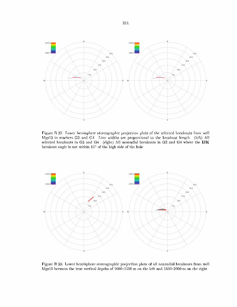
N
S
EW
9.0
18.0
27.0
36.0
45.0
54.0-2485.3
-2410.4N
S
EW
9.0
18.0
27.0
36.0
45.0
54.0-2485.3
-2410.4
Figure B Lower hemisphere stereographic projection plots of the selected breakouts from wellMgs in markers G and G Line widths are proportional to the breakout length left Allselected breakouts in G and G right All nonradial breakouts in G and G where the IJKbreakout angle is not within of the high side of the hole
N
S
EW
9.0
18.0
27.0
36.0
45.0
54.0-1344.9
-1344.9N
S
EW
9.0
18.0
27.0
36.0
45.0
54.0-1975.5
-1947.3
Figure B Lower hemisphere stereographic projection plots of all nonradial breakouts from wellMgs between the true vertical depths of m on the left and m on the right

N
S
EW
9.0
18.0
27.0
36.0
45.0
54.0-2485.3
-2358.1
Figure B Lower hemisphere stereographic projection plots of all nonradial breakouts from wellMgs between the true vertical depths of m

B Mgs
A single paper lowangle dipmeter log covering the log depth range m for Middle Ground
Shoals was received fromUnocal The breakouts from this log were selected by eye The properties
of each breakout were entered into the computer to have the computer select only those breakouts
that met the breakout selection criteria The deviations between the directional survey and the
dipmeter di er at most by with an average di erence of The deviations of this hole reach
but the well log starts at a depth of m below which the maximum borehole deviation is
The borehole azimuth calculated from the dipmeter di ers on average from the directional
surveys borehole azimuth by The maximum di erence between the two azimuths is
The breakout selection scheme identied m of breakouts in the m of well log representing
roughly of the length of the hole These are shown in Figures B and B along with those
breakouts that have IJK breakout angles that di er from the high side or low side of the hole by
Figure B shows the breakouts separated into m true vertical depth intervals Of the oil pools
examined for breakouts only the G and G oil pools had any appreciable borehole elongations
Figure B
The average breakout length was m which is why there are only data points on the
stereonet plots for this hole However the breakout directions are quite inconsistent and there are
too few breakouts to analyze subsets of them The breakouts occur over a relatively small m
true vertical depth interval No faults were listed in the marker le to account for this pattern A
visual estimate of the stress implications of this breakout pattern would have a normal faulting stress
state with the largest principal stress direction oriented roughly NE at a deviation of There
are no faults listed in the marker le that this well crosses that could account for this variability

21.5
22.0
22.5
23.0
23.5
24.0
24.5
25.0
25.5
26.0
Cal
iper
Arm
s (c
entim
eter
s)
2750 2800 2850 2900 2950 3000
Log Depth (meters)
0.00.51.0
Cal
iper
Arm
s (c
entim
eter
s)
0
Log Depth (meters)
21.5
22.0
22.5
23.0
23.5
24.0
24.5
25.0
25.5
26.0
2750 2800 2850 2900 2950 3000
0.00.51.00
21.5
22.0
22.5
23.0
23.5
24.0
24.5
25.0
25.5
26.0
2750 2800 2850 2900 2950 3000
0.00.51.00
21.5
22.0
22.5
23.0
23.5
24.0
24.5
25.0
25.5
26.0
2750 2800 2850 2900 2950 3000
0.00.51.00
21.5
22.0
22.5
23.0
23.5
24.0
24.5
25.0
25.5
26.0
2750 2800 2850 2900 2950 3000
0.00.51.00
21.5
22.0
22.5
23.0
23.5
24.0
24.5
25.0
25.5
26.0
2750 2800 2850 2900 2950 3000
0.00.51.00
20
21
22
23
24
25
26
27
28
29
Dev
iatio
n (d
egre
es)
2750 2800 2850 2900 2950 3000
G2
G3
G4
G5
01
Dev
iatio
n (d
egre
es)
0
20
21
22
23
24
25
26
27
28
29
2750 2800 2850 2900 2950 3000
010
0
100
200
300
400
Azi
mut
hs (
degr
ees)
2750 2800 2850 2900 2950 3000
0
Azi
mut
hs (
degr
ees)
0
0
100
200
300
400
2750 2800 2850 2900 2950 3000
00
0
100
200
300
400
2750 2800 2850 2900 2950 3000
00
0
100
200
300
400
2750 2800 2850 2900 2950 3000
00
0
100
200
300
400
2750 2800 2850 2900 2950 3000
00
0
100
200
300
400
2750 2800 2850 2900 2950 3000
00
0
100
200
300
400
2750 2800 2850 2900 2950 3000
00
Figure B Plots of the calipercalibrated and declinationcorrected selected breakout data as afunction of well depth from well Mgs top Borehole azimuth dashed line with triangles padazimuth dotted line with stars and breakout azimuth solid line with circles middle Boreholedeviation solid line and location of marker horizons vertical lines with labels bottom Caliperarm solid line with hexagons caliper arm dotted line with inverted triangles and bit sizerelatively constant solid line

N
S
EW
9.0
18.0
27.0
36.0
45.0
54.0-2545
-2359.2N
S
EW
9.0
18.0
27.0
36.0
45.0
54.0-2545
-2359.2
Figure B Lower hemisphere stereographic projection plots of the selected breakouts from wellMgs Line widths are proportional to the breakout length left All selected breakouts rightAll nonradial breakouts where the IJK breakout angle is not within of the high side of the hole
N
S
EW
9.0
18.0
27.0
36.0
45.0
54.0-2545
-2417.5N
S
EW
9.0
18.0
27.0
36.0
45.0
54.0-2545
-2417.5
Figure B Lower hemisphere stereographic projection plots of the selected breakouts from wellMgs in markers G and G Line widths are proportional to the breakout length left Allselected breakouts in G and G right All nonradial breakouts in G and G where the IJKbreakout angle is not within of the high side of the hole
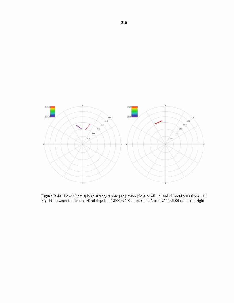
N
S
EW
9.0
18.0
27.0
36.0
45.0
54.0-2417.5
-2359.2N
S
EW
9.0
18.0
27.0
36.0
45.0
54.0-2545
-2545
Figure B Lower hemisphere stereographic projection plots of all nonradial breakouts from wellMgs between the true vertical depths of m on the left and m on the right

B Mgs
Unocal provided a single paper highangle dipmeter log covering the log depth range m
for Middle Ground Shoals was received from Unocal The paper log was examined by eye for
breakouts and the selected breakouts were entered into the computer for automated processing and
again passed through the breakout selection scheme to make sure that the breakouts had satised
all of the criteria The average di erence between the dipmeter and directional survey deviation
is with a maximum di erence of The di erence between the dipmeter and directional
survey borehole azimuth ranged from to
About of the dipmeter log m had borehole elongations The average breakout length
was m All of the breakouts and the nonradial breakouts are shown in Figure B while the same
breakouts plotted in m intervals are shown in Figure B Breakouts were found in all of the
markers that were specically chosen for examination BSS breakouts for m Figure B
D breakouts for m Figure B and G and G breakout for m Figure B The
other markers that had breakouts were breakout for m ASS breakouts for m
B breakouts for m C breakouts for m and G breakout for m
This data set appears to be one of the two breakout data sets that clearly has radial and nonradial
components where the nonradial component has a well dened breakout pattern the other being
Mgs The nonradial breakouts appear to rotate about a breakout nodal point located at an
azimuth of SE deviating roughly Unfortunately part of the breakout pattern for this nodal
point includes breakouts that are radially oriented and will not be included in the nonradial stress
inversions performed

31
32
33
34
35
36
37
38
39
Cal
iper
Arm
s (c
entim
eter
s)
1000 1500 2000 2500 3000
Log Depth (meters)
01
Cal
iper
Arm
s (c
entim
eter
s)
0
Log Depth (meters)
31
32
33
34
35
36
37
38
39
1000 1500 2000 2500 3000
010
31
32
33
34
35
36
37
38
39
1000 1500 2000 2500 3000
010
31
32
33
34
35
36
37
38
39
1000 1500 2000 2500 3000
010
31
32
33
34
35
36
37
38
39
1000 1500 2000 2500 3000
010
31
32
33
34
35
36
37
38
39
1000 1500 2000 2500 3000
010
0
10
20
30
40
Dev
iatio
n (d
egre
es)
1000 1500 2000 2500 3000
36ss
B36ss
38
40
40ss
B40ss
A49sseq
A50ss
A50ass
A51ss
B
C
D
E
F
G1
G2
G3
G4
G5
Twf
0
Dev
iatio
n (d
egre
es)
0
0
10
20
30
40
1000 1500 2000 2500 3000
00
0
50
100
150
200
250
300
350
Azi
mut
hs (
degr
ees)
1000 1500 2000 2500 3000
0
Azi
mut
hs (
degr
ees)
0
0
50
100
150
200
250
300
350
1000 1500 2000 2500 3000
00
0
50
100
150
200
250
300
350
1000 1500 2000 2500 3000
00
0
50
100
150
200
250
300
350
1000 1500 2000 2500 3000
00
0
50
100
150
200
250
300
350
1000 1500 2000 2500 3000
00
0
50
100
150
200
250
300
350
1000 1500 2000 2500 3000
00
0
50
100
150
200
250
300
350
1000 1500 2000 2500 3000
00
Figure B Plots of the calipercalibrated and declinationcorrected selected breakout data as afunction of well depth from well Mgs top Borehole azimuth dashed line with triangles padazimuth dotted line with stars and breakout azimuth solid line with circles middle Boreholedeviation solid line and location of marker horizons vertical lines with labels bottom Caliperarm solid line with hexagons caliper arm dotted line with inverted triangles and bit sizerelatively constant solid line
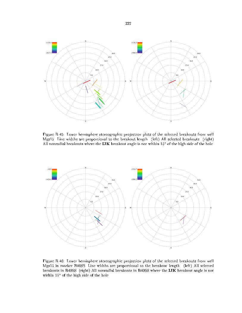
N
S
EW
9.0
18.0
27.0
36.0
45.0
54.0-2627.5
-1116.4N
S
EW
9.0
18.0
27.0
36.0
45.0
54.0-1988.9
-1116.4
Figure B Lower hemisphere stereographic projection plots of the selected breakouts from wellMgs Line widths are proportional to the breakout length left All selected breakouts rightAll nonradial breakouts where the IJK breakout angle is not within of the high side of the hole
N
S
EW
9.0
18.0
27.0
36.0
45.0
54.0-1624.8
-1421N
S
EW
9.0
18.0
27.0
36.0
45.0
54.0-1588.2
-1524.7
Figure B Lower hemisphere stereographic projection plots of the selected breakouts from wellMgs in marker BSS Line widths are proportional to the breakout length left All selectedbreakouts in BSS right All nonradial breakouts in BSS where the IJK breakout angle is notwithin of the high side of the hole

N
S
EW
9.0
18.0
27.0
36.0
45.0
54.0-2126.4
-2026.6N
S
EW
9.0
18.0
27.0
36.0
45.0
54.0
Figure B Lower hemisphere stereographic projection plots of the selected breakouts from wellMgs in marker D Line widths are proportional to the breakout length left All selected breakoutsin D right All nonradial breakouts in D where the IJK breakout angle is not within of thehigh side of the hole
N
S
EW
9.0
18.0
27.0
36.0
45.0
54.0-2627.5
-2627.5N
S
EW
9.0
18.0
27.0
36.0
45.0
54.0
Figure B Lower hemisphere stereographic projection plots of the selected breakouts from wellMgs in markers G and G Line widths are proportional to the breakout length left Allselected breakouts in G and G right All nonradial breakouts in G and G where the IJKbreakout angle is not within of the high side of the hole
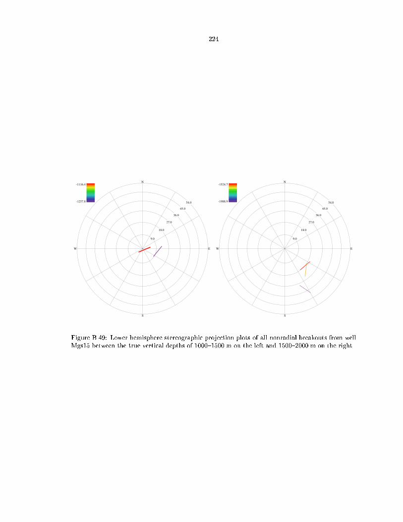
N
S
EW
9.0
18.0
27.0
36.0
45.0
54.0-1257.8
-1116.4N
S
EW
9.0
18.0
27.0
36.0
45.0
54.0-1988.9
-1524.7
Figure B Lower hemisphere stereographic projection plots of all nonradial breakouts from wellMgs between the true vertical depths of m on the left and m on the right

B Mgs
A single lowangle dipmeter paper log was received from Unocal for Middle Ground Shoals This
well log covered the well log depths to m The paper well log was examined by eye for
possible breakouts and the properties of these possible breakouts was entered into the computer
where they were checked by a programmed version of the breakout selection scheme The measured
deviations between the dipmeter and directional survey di er on average by with a maximum
di erence of However the borehole azimuth from the directional survey di ers as much as
from the calculated azimuths from the dipmeter the average di erence is
Out of the m of logged hole m of breakouts were identied in separate breakouts
A plot of the breakout data as a function of depth appears in Figure B Lower hemisphere
stereographic projection plots of the breakouts and the nonradial breakout subset of all of the
breakouts is plotted in Figure B Figures BB show the breakouts separated into m
true vertical depth intervals Breakouts were identied in the three markers that are being specically
examined for the Middle Ground Shoals eld BSS breakouts for m Figure B D
breakout for m Figure B and G with G breakouts for m Figure B Breakouts
were also identied in the following markers breakout for m ASS breakout for
m ASS breakout for m C breakout for m E breakout for m and F
breakouts for m
This log has wellbehaved ingauge sections with tool rotation some washedout sections key
seats and numerous sections that appeared to be wellbehaved breakouts Often these brokenout
sections were quite consistent for long distances and could have been picked less conservatively and
for greater distances down hole than were picked here Because this hole is not highly deviated
the breakout directions particularly in the deepest section of the hole are probably close to what
one would expect to nd in a vertical hole Thus these data can be taken as some indication of the
direction of SH
This hole has two distinct populations of breakouts The shallow set extends to m TVD
and is oriented for the most part between NESW and NNESSW The deeper breakouts of the
shallow set are rotated more clockwise than the shallower breakouts and may represent part of a
radial breakout pattern not centered on the center of the plot The deeper set of three breakouts
starts at m and is oriented just west of north The marker le does not list any faults that
this well crossed Between m and m the transition between the two sets of breakouts
occurs partly in the F marker covers all of the G marker and ends in the G marker
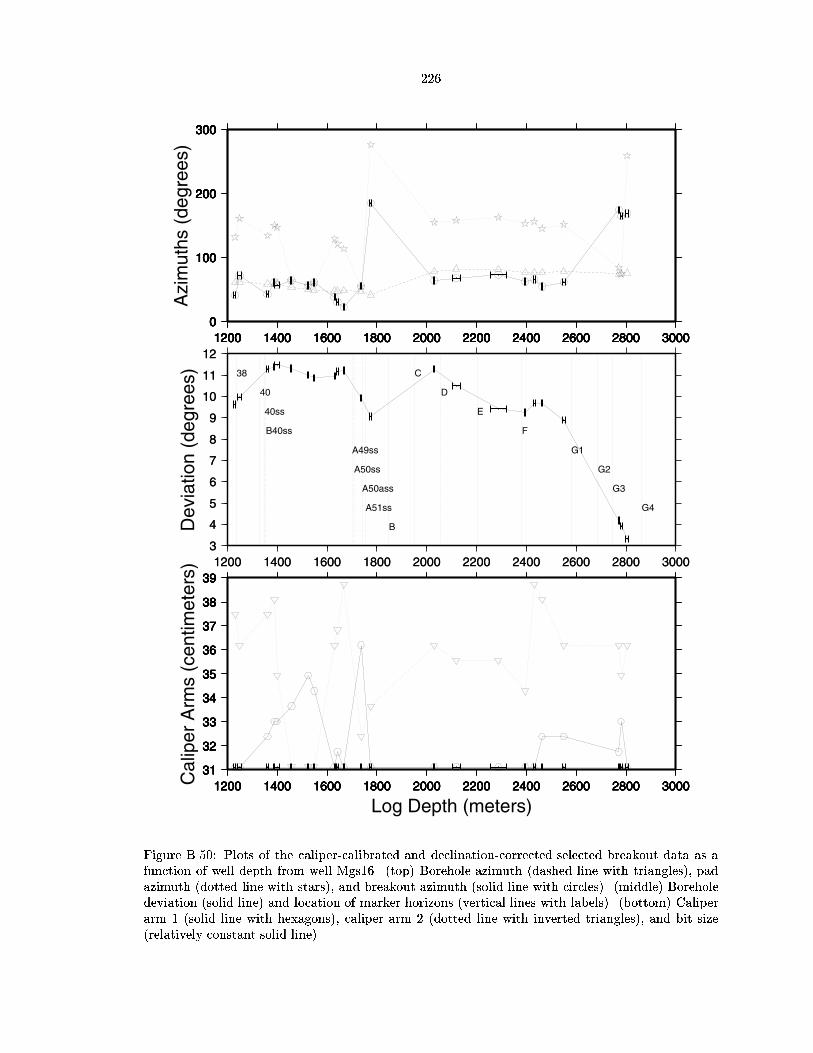
31
32
33
34
35
36
37
38
39
Cal
iper
Arm
s (c
entim
eter
s)
1200 1400 1600 1800 2000 2200 2400 2600 2800 3000
Log Depth (meters)
01
Cal
iper
Arm
s (c
entim
eter
s)
0
Log Depth (meters)
31
32
33
34
35
36
37
38
39
1200 1400 1600 1800 2000 2200 2400 2600 2800 3000
010
31
32
33
34
35
36
37
38
39
1200 1400 1600 1800 2000 2200 2400 2600 2800 3000
010
31
32
33
34
35
36
37
38
39
1200 1400 1600 1800 2000 2200 2400 2600 2800 3000
010
31
32
33
34
35
36
37
38
39
1200 1400 1600 1800 2000 2200 2400 2600 2800 3000
010
31
32
33
34
35
36
37
38
39
1200 1400 1600 1800 2000 2200 2400 2600 2800 3000
010
3
4
5
6
7
8
9
10
11
12
Dev
iatio
n (d
egre
es)
1200 1400 1600 1800 2000 2200 2400 2600 2800 3000
38
40
40ss
B40ss
A49ss
A50ss
A50ass
A51ss
B
C
D
E
F
G1
G2
G3
G4
01
Dev
iatio
n (d
egre
es)
0
3
4
5
6
7
8
9
10
11
12
1200 1400 1600 1800 2000 2200 2400 2600 2800 3000
010
0
100
200
300
Azi
mut
hs (
degr
ees)
1200 1400 1600 1800 2000 2200 2400 2600 2800 3000
0
Azi
mut
hs (
degr
ees)
0
0
100
200
300
1200 1400 1600 1800 2000 2200 2400 2600 2800 3000
00
0
100
200
300
1200 1400 1600 1800 2000 2200 2400 2600 2800 3000
00
0
100
200
300
1200 1400 1600 1800 2000 2200 2400 2600 2800 3000
00
0
100
200
300
1200 1400 1600 1800 2000 2200 2400 2600 2800 3000
00
0
100
200
300
1200 1400 1600 1800 2000 2200 2400 2600 2800 3000
00
0
100
200
300
1200 1400 1600 1800 2000 2200 2400 2600 2800 3000
00
Figure B Plots of the calipercalibrated and declinationcorrected selected breakout data as afunction of well depth from well Mgs top Borehole azimuth dashed line with triangles padazimuth dotted line with stars and breakout azimuth solid line with circles middle Boreholedeviation solid line and location of marker horizons vertical lines with labels bottom Caliperarm solid line with hexagons caliper arm dotted line with inverted triangles and bit sizerelatively constant solid line

N
S
EW
9.0
18.0
27.0
36.0
45.0
54.0-2768.9
-1216.3N
S
EW
9.0
18.0
27.0
36.0
45.0
54.0-2768.9
-1216.3
Figure B Lower hemisphere stereographic projection plots of the selected breakouts from wellMgs Line widths are proportional to the breakout length left All selected breakouts rightAll nonradial breakouts where the IJK breakout angle is not within of the high side of the hole
N
S
EW
9.0
18.0
27.0
36.0
45.0
54.0-1645.8
-1345.1N
S
EW
9.0
18.0
27.0
36.0
45.0
54.0-1645.8
-1621.3
Figure B Lower hemisphere stereographic projection plots of the selected breakouts from wellMgs in marker BSS Line widths are proportional to the breakout length left All selectedbreakouts in BSS right All nonradial breakouts in BSS where the IJK breakout angle is notwithin of the high side of the hole

N
S
EW
9.0
18.0
27.0
36.0
45.0
54.0-2090.6
-2090.6N
S
EW
9.0
18.0
27.0
36.0
45.0
54.0
Figure B Lower hemisphere stereographic projection plots of the selected breakouts from wellMgs in marker D Line widths are proportional to the breakout length left All selected breakoutsin D right All nonradial breakouts in D where the IJK breakout angle is not within of thehigh side of the hole
N
S
EW
9.0
18.0
27.0
36.0
45.0
54.0-2768.9
-2735.7N
S
EW
9.0
18.0
27.0
36.0
45.0
54.0-2768.9
-2735.7
Figure B Lower hemisphere stereographic projection plots of the selected breakouts from wellMgs in markers G and G Line widths are proportional to the breakout length left Allselected breakouts in G and G right All nonradial breakouts in G and G where the IJKbreakout angle is not within of the high side of the hole

N
S
EW
9.0
18.0
27.0
36.0
45.0
54.0-1216.3
-1216.3N
S
EW
9.0
18.0
27.0
36.0
45.0
54.0-1752.4
-1621.3
Figure B Lower hemisphere stereographic projection plots of all nonradial breakouts from wellMgs between the true vertical depths of m on the left and m on the right
N
S
EW
9.0
18.0
27.0
36.0
45.0
54.0-2430.3
-2430.3N
S
EW
9.0
18.0
27.0
36.0
45.0
54.0-2768.9
-2515.7
Figure B Lower hemisphere stereographic projection plots of all nonradial breakouts from wellMgs between the true vertical depths of m on the left and m on the right

B Mgs
Unocal provided digital dipmeter directional survey logs and marker les for Middle Ground Shoals
Figure B This well had deviations up to which made it very promising for providing
stress state information Unfortunately the caliper arms were much smaller than the bit size which
reects the fact that the hole has a large channel dug in the bottom of the hole where the dipmeter
tool lay while logging the hole Rod Paulson personal communication Since the deviations are so
high this is not too surprising Because of the noncircular shape of the hole and the mismatched
caliper arm and bit size data no computer selected breakouts were identied

10
20
30
40
50
Cal
iper
Arm
s (c
entim
eter
s)
600 700 800 900 1000 1100
Log Depth (meters)
0
Cal
iper
Arm
s (c
entim
eter
s)
0
Log Depth (meters)
10
20
30
40
50
600 700 800 900 1000 1100
00
10
20
30
40
50
600 700 800 900 1000 1100
00
10
20
30
40
50
600 700 800 900 1000 1100
00
35
40
45
50
55
60
65
70
75
Dev
iatio
n (d
egre
es)
600 700 800 900 1000 1100
24
24ss
0
Dev
iatio
n (d
egre
es)
0
35
40
45
50
55
60
65
70
75
600 700 800 900 1000 1100
00
0
100
200
300
Azi
mut
hs (
degr
ees)
600 700 800 900 1000 1100
0
Azi
mut
hs (
degr
ees)
0
0
100
200
300
600 700 800 900 1000 1100
00
0
100
200
300
600 700 800 900 1000 1100
00
0
100
200
300
600 700 800 900 1000 1100
00
Figure B Plots of the calipercalibrated and declinationcorrected digitized dipmeter and derivedquantities data as a function of well depth from well Mgs top Borehole elongation directionsolid line pad azimuth dotted line and borehole azimuth dashed line middle Boreholedeviation solid curve and location of marker horizons vertical lines with labels bottom Bit sizestraight solid line caliper arm solid line and caliper arm dotted line Selected breakoutregions are plotted as horizontal bars showing the depth extent of the breakouts

B Mgs
Mgs is the second Middle Ground Shoals well that digital data from both the directional survey
and dipmeter tools was received from Unocal Figure B The type of dipmeter used to log this
hole is unknown The dipmeter logged the well depth interval from to m The deviations
agree within between the directional survey data and the dipmeter data Excluding the top
part of the well log where the borehole deviation is very close to and the borehole azimuth has
no meaning the minimum and maximum di erence between the borehole and dipmeter borehole
azimuths are and respectively The directional survey borehole azimuths are used for
the breakout calculations for this hole
In the m of logged hole separate breakouts were identied totaling m in length
Figure B The same breakouts broken out into m TVD intervals are shown in Figures B
B and the nonradial breakouts are plotted in Figure B Borehole elongations were found in
the C breakouts for m D breakouts for m Figure B E breakouts for m
and F breakouts for m markers
Except for a few breakouts near the bottom of the log this well has a very consistent breakout
pattern of an arc that follows the boreholes trend through orientation space The shallow breakouts
are almost radial while the deeper ones seem to follow the change in the boreholes orientation
However this is probably a coincidence between the boreholes path and the stress state that causes
this pattern of breakouts The maximum rate of change of the boreholes path is m which is
too small to a ect the location of breakouts on the borehole wall
This well is similar to Mgs where one radial breakout pattern overlies a nonradial data with
a clearly dened pattern Figure B Examination of the nonradial breakouts from Mgs in
isolation from breakout data sets seem to show a similar thrust faulting stress state with a nodal
point somewhere east of south at a relatively high deviation This is also similar to Mgss results
The location of the nodal point is less clear here since the breakouts do not change their orientation
very quickly as a function of borehole orientation suggesting that the nodal point is close but not
very close to the breakout data

0
10
20
30
40
50
Cal
iper
Arm
s (c
entim
eter
s)
1700 1800 1900 2000 2100 2200 2300 2400 2500 2600 2700 2800
Log Depth (meters)
0
Cal
iper
Arm
s (c
entim
eter
s)
0
Log Depth (meters)
0
10
20
30
40
50
1700 1800 1900 2000 2100 2200 2300 2400 2500 2600 2700 2800
00
0
10
20
30
40
50
1700 1800 1900 2000 2100 2200 2300 2400 2500 2600 2700 2800
00
0
10
20
30
40
50
1700 1800 1900 2000 2100 2200 2300 2400 2500 2600 2700 2800
00
25
30
35
40
45
50
55
Dev
iatio
n (d
egre
es)
1700 1800 1900 2000 2100 2200 2300 2400 2500 2600 2700 2800
A
B
C
D
E
F
G1
G2
G3
0
Dev
iatio
n (d
egre
es)
0
25
30
35
40
45
50
55
1700 1800 1900 2000 2100 2200 2300 2400 2500 2600 2700 2800
00
0
100
200
300
Azi
mut
hs (
degr
ees)
1700 1800 1900 2000 2100 2200 2300 2400 2500 2600 2700 2800
0
Azi
mut
hs (
degr
ees)
0
0
100
200
300
1700 1800 1900 2000 2100 2200 2300 2400 2500 2600 2700 2800
00
0
100
200
300
1700 1800 1900 2000 2100 2200 2300 2400 2500 2600 2700 2800
00
0
100
200
300
1700 1800 1900 2000 2100 2200 2300 2400 2500 2600 2700 2800
00
Figure B Plots of the calipercalibrated and declinationcorrected digitized dipmeter and derivedquantities data as a function of well depth from well Mgs top Borehole elongation directionsolid line pad azimuth dotted line and borehole azimuth dashed line middle Boreholedeviation solid curve and location of marker horizons vertical lines with labels bottom Bit sizestraight solid line caliper arm solid line and caliper arm dotted line Selected breakoutregions are plotted as horizontal bars showing the depth extent of the breakouts

N
S
EW
9.0
18.0
27.0
36.0
45.0
54.0-2501.1
-1984.5N
S
EW
9.0
18.0
27.0
36.0
45.0
54.0-2485.6
-1984.5
Figure B Lower hemisphere stereographic projection plots of the selected breakouts from wellMgs Line widths are proportional to the breakout length left All selected breakouts rightAll nonradial breakouts where the IJK breakout angle is not within of the high side of the hole
N
S
EW
9.0
18.0
27.0
36.0
45.0
54.0-2156.8
-2002.6N
S
EW
9.0
18.0
27.0
36.0
45.0
54.0-2143.1
-2002.6
Figure B Lower hemisphere stereographic projection plots of the selected breakouts from wellMgs in marker D Line widths are proportional to the breakout length left All selected breakoutsin D right All nonradial breakouts in D where the IJK breakout angle is not within of thehigh side of the hole

N
S
EW
9.0
18.0
27.0
36.0
45.0
54.0-1984.5
-1984.5N
S
EW
9.0
18.0
27.0
36.0
45.0
54.0-2485.6
-2002.6
Figure B Lower hemisphere stereographic projection plots of all nonradial breakouts from wellMgs between the true vertical depths of m on the left and m on the right
N
S
EW
9.0
18.0
27.0
36.0
45.0
54.0
Figure B Lower hemisphere stereographic projection plots of all nonradial breakouts from wellMgs between the true vertical depths of m

B Mgs
Unocal provided digital dipmeter and directional survey les for Middle Ground Shoals Mgs
Figure B It is unclear whether a lowangle or highangle dipmeter was used to log this hole but
it could have been a lowangle unit since the deviations do not reach The borehole deviations
range from up to The maximum di erence between the dipmeter and directional survey
in terms of borehole deviation is The borehole azimuth as measured by the dipmeter di ers
on average by from the borehole azimuth as measured by the directional survey with the
maximum di erence being
Figure B shows all the breakouts identied in this hole and the nonradial subset of these
breakouts plotted separately The marker le for this hole only listed two markers F and G both
of which had horizon tops deeper than the deepest identied breakout
There are two populations of breakouts a shallow set of three EW to ESEWNW breakouts
and a deeper set of breakouts which have a large variation in breakout azimuth There is a large
change in the bit size between the shallow and deeper portions of the hole at m log depth
Figure B The shallow portion was drilled with a larger bit size cm or inches and
the deeper portion was drilled with a smaller bit size cm or inches The change in
bit size does not distinguish the change in the two populations of breakouts since the shallowest
breakout from the deeper set of breakouts was identied in the section of the hole drilled with the
larger bit
The three breakouts in the shallow set have azimuths between NE and NE The
deeper set of breakouts may be consistent with a nodal point located at a slightly higher deviation
than the lowest deviation breakouts If this were the case then the breakouts would constrain a
thrust faulting stress state Figure and the nodal point would match the nodal points found
in the Mgs and Mgs wells The resulting stress state would have NNWSSE trending maxi
mum horizontal principal stress direction This interpretation also matches the interpretation from
Mgs Figure B which shows breakouts at roughly the same position on the lower hemisphere
stereographic projection plots The possibility of this data suggesting this result will be examined
later in conjunction with all of the data in Cook Inlet

20
30
40
50
Cal
iper
Arm
s (c
entim
eter
s)
600 800 1000 1200 1400 1600 1800 2000 2200
Log Depth (meters)
0
Cal
iper
Arm
s (c
entim
eter
s)
0
Log Depth (meters)
20
30
40
50
600 800 1000 1200 1400 1600 1800 2000 2200
00
20
30
40
50
600 800 1000 1200 1400 1600 1800 2000 2200
00
20
30
40
50
600 800 1000 1200 1400 1600 1800 2000 2200
00
5
10
15
20
25
30
35
Dev
iatio
n (d
egre
es)
600 800 1000 1200 1400 1600 1800 2000 2200
0
Dev
iatio
n (d
egre
es)
0
5
10
15
20
25
30
35
600 800 1000 1200 1400 1600 1800 2000 2200
00
0
100
200
300
400
Azi
mut
hs (
degr
ees)
600 800 1000 1200 1400 1600 1800 2000 2200
0
Azi
mut
hs (
degr
ees)
0
0
100
200
300
400
600 800 1000 1200 1400 1600 1800 2000 2200
00
0
100
200
300
400
600 800 1000 1200 1400 1600 1800 2000 2200
00
0
100
200
300
400
600 800 1000 1200 1400 1600 1800 2000 2200
00
Figure B Plots of the calipercalibrated and declinationcorrected digitized dipmeter and derivedquantities data as a function of well depth from well Mgs top Borehole elongation directionsolid line pad azimuth dotted line and borehole azimuth dashed line middle Boreholedeviation solid curve and location of marker horizons vertical lines with labels bottom Bit sizestraight solid line caliper arm solid line and caliper arm dotted line Selected breakoutregions are plotted as horizontal bars showing the depth extent of the breakouts

N
S
EW
9.0
18.0
27.0
36.0
45.0
54.0-1931.7
-614.9N
S
EW
9.0
18.0
27.0
36.0
45.0
54.0-1931.7
-614.9
Figure B Lower hemisphere stereographic projection plots of the selected breakouts from wellMgs Line widths are proportional to the breakout length left All selected breakouts rightAll nonradial breakouts where the IJK breakout angle is not within of the high side of the hole
N
S
EW
9.0
18.0
27.0
36.0
45.0
54.0-626.8
-614.9N
S
EW
9.0
18.0
27.0
36.0
45.0
54.0-1931.7
-1650.9
Figure B Lower hemisphere stereographic projection plots of all nonradial breakouts from wellMgs between the true vertical depths of m on the left and m on the right

B Smgs
One paper well log for Smgs that logged the depth range m to m log depth was received
from Unocal The paper well log was digitized by hand and breakouts were selected according to the
breakout selection criteria for the Cook Inlet data The digitized data and the selected breakouts
are shown in Figure B The largest deviation from this dipmeter log was The caliper arm
data has a lot of variation over the entire depth range including a large amount of key seats Thirty
ingauge sections of hole longer than m were found totaling m in length
Over the whole well log breakouts with a total length of m were identied The lower
hemisphere stereographic projection plot of the breakouts shows a general trend of NS directed
shallow breakouts that rotate to NESW at the deep end of the hole Figure B The trend has a
large amount of variability to it There are thirteen breakouts that have IJK breakout angles that
di er by at least from the next shallower IJK breakout angle Nine of these occur when the
adjacent breakouts occur in di erent markers and the rest occur in the same marker The largest
IJK angle di erence of occurs between two breakouts separated by m in the T marker
The high variability in the breakout angles will produce a poorer inversion t but none of the
identied breakouts will be removed from the data set since I do not have that much information
on the markers this well passes through
The nonradial breakouts selected into m TVD depth intervals are plotted in Figures B
B Three breakouts were identied in the TE marker the marker chosen for examination
of breakout azimuths in a single marker for the Dillon platform breakouts Figure B Other
breakouts were found in the following markers T breakouts for m T breakouts for
m T breakouts for m T breakouts for m T breakout for m T
breakout for m T breakouts for m T breakouts for m T breakout
for m T breakouts for m T breakouts for m T breakouts for m
T breakout for m T breakout for m TA breakouts for m BC
breakout for m TC breakouts for m BD breakout for m T breakout
for m and TE breakouts for m Not all of the breakouts are listed here since some of
them lie in unidentied markers

10
20
30
40
50
Cal
iper
Arm
s (c
entim
eter
s)
800 1000 1200 1400 1600 1800 2000 2200 2400 2600 2800 3000 3200
Log Depth (meters)
0
Cal
iper
Arm
s (c
entim
eter
s)
0
Log Depth (meters)
10
20
30
40
50
800 1000 1200 1400 1600 1800 2000 2200 2400 2600 2800 3000 3200
00
10
20
30
40
50
800 1000 1200 1400 1600 1800 2000 2200 2400 2600 2800 3000 3200
00
10
20
30
40
50
800 1000 1200 1400 1600 1800 2000 2200 2400 2600 2800 3000 3200
00
20
25
30
35
40
Dev
iatio
n (d
egre
es)
800 1000 1200 1400 1600 1800 2000 2200 2400 2600 2800 3000 3200
T2
T3
T7
T8
T9
T10
T11
T12
T13
T14
T16
T17
T18
T19
T20
T21
T22
T23
T24
T26
T2627ss
B2627ss
Ta2
T34
Tb1
T36
Tc1
Bc2
Tc3
Bd2
C58
T40
Te1
T42
Tf1
T44
Them
0
Dev
iatio
n (d
egre
es)
0
20
25
30
35
40
800 1000 1200 1400 1600 1800 2000 2200 2400 2600 2800 3000 3200
00
0
100
200
300
400
Azi
mut
hs (
degr
ees)
800 1000 1200 1400 1600 1800 2000 2200 2400 2600 2800 3000 3200
0
Azi
mut
hs (
degr
ees)
0
0
100
200
300
400
800 1000 1200 1400 1600 1800 2000 2200 2400 2600 2800 3000 3200
00
0
100
200
300
400
800 1000 1200 1400 1600 1800 2000 2200 2400 2600 2800 3000 3200
00
0
100
200
300
400
800 1000 1200 1400 1600 1800 2000 2200 2400 2600 2800 3000 3200
00
Figure B Plots of the calipercalibrated and declinationcorrected digitized dipmeter and derivedquantities data as a function of well depth from well Smgs top Borehole elongation directionsolid line pad azimuth dotted line and borehole azimuth dashed line middle Boreholedeviation solid curve and location of marker horizons vertical lines with labels bottom Bit sizestraight solid line caliper arm solid line and caliper arm dotted line Selected breakoutregions are plotted as horizontal bars showing the depth extent of the breakouts

N
S
EW
9.0
18.0
27.0
36.0
45.0
54.0-2708.7
-948.8N
S
EW
9.0
18.0
27.0
36.0
45.0
54.0-2708.7
-948.8
Figure B Lower hemisphere stereographic projection plots of the selected breakouts from wellSmgs Line widths are proportional to the breakout length left All selected breakouts rightAll nonradial breakouts where the IJK breakout angle is not within of the high side of the hole
N
S
EW
9.0
18.0
27.0
36.0
45.0
54.0-2708.7
-2693.8N
S
EW
9.0
18.0
27.0
36.0
45.0
54.0-2708.7
-2693.8
Figure B Lower hemisphere stereographic projection plots of the selected breakouts from wellSmgs in marker TE Line widths are proportional to the breakout length left All selectedbreakouts in TE right All nonradial breakouts in TE where the IJK breakout angle is notwithin of the high side of the hole

N
S
EW
9.0
18.0
27.0
36.0
45.0
54.0-976.8
-948.8N
S
EW
9.0
18.0
27.0
36.0
45.0
54.0-1102.9
-1010.4
Figure B Lower hemisphere stereographic projection plots of all nonradial breakouts from wellSmgs between the true vertical depths of m on the left and m on the right
N
S
EW
9.0
18.0
27.0
36.0
45.0
54.0-1931.7
-1503.5N
S
EW
9.0
18.0
27.0
36.0
45.0
54.0-2172.1
-2011.7
Figure B Lower hemisphere stereographic projection plots of all nonradial breakouts from wellSmgs between the true vertical depths of m on the left and m on the right

N
S
EW
9.0
18.0
27.0
36.0
45.0
54.0-2708.7
-2588.1
Figure B Lower hemisphere stereographic projection plots of all nonradial breakouts from wellSmgs between the true vertical depths of m

B Smgs
Unocal provided one paper dipmeter log for South Middle Ground Shoals A well log digitizing
company was hired by Unocal to digitize the paper log and they digitized the caliper arm deviation
relative bearing and pad azimuth data The digitized caliper arm data was o set from the real
caliper arm measurements on the paper log From examining several caliper arm measurements
between the digitized data and the paper log it appeared that the digitized data was cm
inches larger than the paper log values An additive o set of cm was applied to the
digitized caliper arm data before any further processing The nal processed digital data is plotted
in Figure B The digitized data spanned the log depth range from m to m The
highest measured deviations in the dipmeter data was A lowangle dipmeter tool was used to
log this hole There are m of ingauge hole at least m long However the pad azimuth
shows a large amount of tool rotation in this hole
The breakout selection criteria identied breakouts which have a combined length of m
No breakouts were found in the TE marker which was selected for the Dillon platform wells as a
particular marker to study breakouts in Nine breakouts spanning m were identied in the C
marker and the remaining breakouts were not located in any marker since the marker le did not
cover the complete depth range spanned by the well log The data are plotted on a lower hemisphere
stereographic projection plot in Figure B along with breakouts that have an IJK breakout angle
more than away from the high or low side of the hole The borehole breakout orientations have
a large degree of variability There are sections of the hole where the breakout orientations are more
consistent but even some of these have a large angular distribution of orientation
It appears that a combination of two e ects caused the breakout orientation variability The
rst is that dipmeter rotated only six times completely around over the m section of hole top
of Figure B The second factor is that the borehole breakout selection scheme was not strict
enough for this well The combination of the two factors caused breakouts to be identied at almost
every azimuth Even the breakouts observed in some of the m TVD intervals show a similar
amount of breakout azimuth variation Figures BB
To examine if the breakout selection scheme criteria were not strict enough for this well the
data set was examined using two di erent methods The rst method made the breakout selection
criteria tighter by halving the maximum allowed IJK breakout angle variation over the length of
the breakout to The second test was to take the original set of breakouts and examine the
paper log where the computer selected breakouts were identied and remove those breakouts by eye
that did not meet the criteria that were used to pick the Middle Ground Shoals breakouts by eye
Both tests did not lead to an improvement in the breakout azimuth variability by discarding those
breakouts that may have been spurious in the data set

15
20
25
30
35
40
45
50
Cal
iper
Arm
s (c
entim
eter
s)
500 1000 1500 2000 2500 3000 3500
Log Depth (meters)
0
Cal
iper
Arm
s (c
entim
eter
s)
0
Log Depth (meters)
15
20
25
30
35
40
45
50
500 1000 1500 2000 2500 3000 3500
00
15
20
25
30
35
40
45
50
500 1000 1500 2000 2500 3000 3500
00
15
20
25
30
35
40
45
50
500 1000 1500 2000 2500 3000 3500
00
1
2
3
4
5
Dev
iatio
n (d
egre
es)
500 1000 1500 2000 2500 3000 3500
C58
01
Dev
iatio
n (d
egre
es)
0
1
2
3
4
5
500 1000 1500 2000 2500 3000 3500
010
0
100
200
300
400
Azi
mut
hs (
degr
ees)
500 1000 1500 2000 2500 3000 3500
0
Azi
mut
hs (
degr
ees)
0
0
100
200
300
400
500 1000 1500 2000 2500 3000 3500
00
0
100
200
300
400
500 1000 1500 2000 2500 3000 3500
00
0
100
200
300
400
500 1000 1500 2000 2500 3000 3500
00
Figure B Plots of the calipercalibrated and declinationcorrected digitized dipmeter and derivedquantities data as a function of well depth from well Smgs top Borehole elongation directionsolid line pad azimuth dotted line and borehole azimuth dashed line middle Boreholedeviation solid curve and location of marker horizons vertical lines with labels bottom Bit sizestraight solid line caliper arm solid line and caliper arm dotted line Selected breakoutregions are plotted as horizontal bars showing the depth extent of the breakouts

Through examining the data it does not appear that there are any di erentiating factors which
would help discern a particular breakout direction as being the correct breakout direction The
only possible explanation for this pattern from a stress state interpretation is that the local stress
state near the borehole is near a degenerate thrust or normal stress state when or It
was shown in Figure that the theoretical breakout pattern for a well drilled parallel to one of the
principal stress directions for a degenerate stress state will have widely varying breakout azimuths
for small changes of the borehole azimuth and deviation
The marker le for this well lists only a single horizon named C at m log depth so
no interpretations of the breakouts are possible using this information It has been shown that the
compressive stress direction perpendicular to the anticlines fold axis varies with position due to the
exural strain in the fold Bruno and Winterstein It is expected for a vertical well drilled
into the crest of an anticline that the shallower breakouts would demonstrate a stress direction more
aligned with the anticlines fold axis as compared to the deeper breakouts If there is bedding plane
slip between the beds the well crosses then a pattern would emerge where the breakouts in the
deeper sections of beds would show maximum horizontal stress directions more perpendicular to the
fold axis and shallower breakouts would show maximum horizontal principal stress directions aligned
with the anticlines fold axis The breakout pattern would ip between two endpoint azimuths and
this is not observed It appears then that these breakouts are simply poorly identied borehole
elongations and the data from this well will not be included in any stress state inversions
N
S
EW
9.0
18.0
27.0
36.0
45.0
54.0-2868.2
-839.4N
S
EW
9.0
18.0
27.0
36.0
45.0
54.0-2868.2
-839.4
Figure B Lower hemisphere stereographic projection plots of the selected breakouts from wellSmgs Line widths are proportional to the breakout length left All selected breakouts rightAll nonradial breakouts where the IJK breakout angle is not within of the high side of the hole

N
S
EW
9.0
18.0
27.0
36.0
45.0
54.0-988.5
-839.4N
S
EW
9.0
18.0
27.0
36.0
45.0
54.0-1422.5
-1011
Figure B Lower hemisphere stereographic projection plots of all nonradial breakouts from wellSmgs between the true vertical depths of m on the left and m on the right
N
S
EW
9.0
18.0
27.0
36.0
45.0
54.0-1994.7
-1549.7N
S
EW
9.0
18.0
27.0
36.0
45.0
54.0-2469.3
-2072.4
Figure B Lower hemisphere stereographic projection plots of all nonradial breakouts from wellSmgs between the true vertical depths of m on the left and m on the right

N
S
EW
9.0
18.0
27.0
36.0
45.0
54.0-2868.2
-2524.5
Figure B Lower hemisphere stereographic projection plots of all nonradial breakouts from wellSmgs between the true vertical depths of m

B Smgs
The paper well log for South Middle Ground Shoals spans the log depth range m The
well log was digitized by hand into the computer for computer selected breakouts Figure B
The maximum deviation of the hole in this well log was Ingauge sections of the hole longer
than m accounted for m or of the length of logged hole
Only a single breakout m long was identied at m TVD in the TC marker It
has roughly an azimuth orientation to it Figure B Identifying only one breakout is not too
surprising given that much of the caliper arm data was less than the bit size Figure B
N
S
EW
9.0
18.0
27.0
36.0
45.0
54.0-2444.4
-2444.4N
S
EW
9.0
18.0
27.0
36.0
45.0
54.0-2444.4
-2444.4
Figure B Lower hemisphere stereographic projection plots of the selected breakouts from wellSmgs Line widths are proportional to the breakout length left All selected breakouts rightAll nonradial breakouts where the IJK breakout angle is not within of the high side of the hole

22
24
26
28
30
32
34
36
38
Cal
iper
Arm
s (c
entim
eter
s)
2600 2700 2800 2900 3000 3100 3200 3300
Log Depth (meters)
0
Cal
iper
Arm
s (c
entim
eter
s)
0
Log Depth (meters)
22
24
26
28
30
32
34
36
38
2600 2700 2800 2900 3000 3100 3200 3300
00
22
24
26
28
30
32
34
36
38
2600 2700 2800 2900 3000 3100 3200 3300
00
22
24
26
28
30
32
34
36
38
2600 2700 2800 2900 3000 3100 3200 3300
00
12
13
14
15
16
17
18
19
20
Dev
iatio
n (d
egre
es)
2600 2700 2800 2900 3000 3100 3200 3300
Tc1
Te1
C58
Tf1
Them
01
Dev
iatio
n (d
egre
es)
0
12
13
14
15
16
17
18
19
20
2600 2700 2800 2900 3000 3100 3200 3300
010
0
100
200
300
400
Azi
mut
hs (
degr
ees)
2600 2700 2800 2900 3000 3100 3200 3300
0
Azi
mut
hs (
degr
ees)
0
0
100
200
300
400
2600 2700 2800 2900 3000 3100 3200 3300
00
0
100
200
300
400
2600 2700 2800 2900 3000 3100 3200 3300
00
0
100
200
300
400
2600 2700 2800 2900 3000 3100 3200 3300
00
Figure B Plots of the calipercalibrated and declinationcorrected digitized dipmeter and derivedquantities data as a function of well depth from well Smgs top Borehole elongation directionsolid line pad azimuth dotted line and borehole azimuth dashed line middle Boreholedeviation solid curve and location of marker horizons vertical lines with labels bottom Bit sizestraight solid line caliper arm solid line and caliper arm dotted line Selected breakoutregions are plotted as horizontal bars showing the depth extent of the breakouts

B Smgs
The dipmeter data for South Middle Ground Shoals consists of a single paper well log which was
digitized into the computer Figure B The dipmeter log extends from to m The
maximum observed borehole deviation in this section of hole is Ingauge sections of the hole
longer than m accounted for m of the length of the hole
Eleven breakouts totaling m in length were identied in this section of hole All but two of
the eleven breakouts are within of the high or low side of the hole Figure B Four of the
identied breakouts occurred in the TE marker and all four are within of the high side of the
hole Figure B The remaining breakouts occurs in the TC breakout for m and THEM
breakouts for m markers
Since there are only two nonradial breakouts they are not plotted separately in m TVD
intervals

10
20
30
40
50
Cal
iper
Arm
s (c
entim
eter
s)
3200 3300 3400 3500 3600 3700 3800 3900 4000
Log Depth (meters)
0
Cal
iper
Arm
s (c
entim
eter
s)
0
Log Depth (meters)
10
20
30
40
50
3200 3300 3400 3500 3600 3700 3800 3900 4000
00
10
20
30
40
50
3200 3300 3400 3500 3600 3700 3800 3900 4000
00
10
20
30
40
50
3200 3300 3400 3500 3600 3700 3800 3900 4000
00
38
39
40
41
42
43
Dev
iatio
n (d
egre
es)
3200 3300 3400 3500 3600 3700 3800 3900 4000
Tb1
Tc1
Tc3
C58
Te1
Tf1
Them
01
Dev
iatio
n (d
egre
es)
0
38
39
40
41
42
43
3200 3300 3400 3500 3600 3700 3800 3900 4000
010
0
100
200
300
400
Azi
mut
hs (
degr
ees)
3200 3300 3400 3500 3600 3700 3800 3900 4000
0
Azi
mut
hs (
degr
ees)
0
0
100
200
300
400
3200 3300 3400 3500 3600 3700 3800 3900 4000
00
0
100
200
300
400
3200 3300 3400 3500 3600 3700 3800 3900 4000
00
0
100
200
300
400
3200 3300 3400 3500 3600 3700 3800 3900 4000
00
Figure B Plots of the calipercalibrated and declinationcorrected digitized dipmeter and derivedquantities data as a function of well depth from well Smgs top Borehole elongation directionsolid line pad azimuth dotted line and borehole azimuth dashed line middle Boreholedeviation solid curve and location of marker horizons vertical lines with labels bottom Bit sizestraight solid line caliper arm solid line and caliper arm dotted line Selected breakoutregions are plotted as horizontal bars showing the depth extent of the breakouts

N
S
EW
9.0
18.0
27.0
36.0
45.0
54.0-3028.5
-2631.6N
S
EW
9.0
18.0
27.0
36.0
45.0
54.0-3028.5
-2955.4
Figure B Lower hemisphere stereographic projection plots of the selected breakouts from wellSmgs Line widths are proportional to the breakout length left All selected breakouts rightAll nonradial breakouts where the IJK breakout angle is not within of the high side of the hole
N
S
EW
9.0
18.0
27.0
36.0
45.0
54.0-2737
-2721.9N
S
EW
9.0
18.0
27.0
36.0
45.0
54.0
Figure B Lower hemisphere stereographic projection plots of the selected breakouts from wellSmgs in marker TE Line widths are proportional to the breakout length left All selectedbreakouts in TE right All nonradial breakouts in TE where the IJK breakout angle is notwithin of the high side of the hole

Bibliography
Aadnoy B S Inversion technique to determine the insitu stress eld from fracturing data J Pet
Sci Eng a
Aadnoy B S Insitu stress direction from borehole fracture traces J Pet Sci Eng
b
Addis T D Boulter L RocaRamisa and D Plumb The quest for borehole stability in the
Cusiana Field Columbia Oileld Review
Angelier J Tectonic analysis of fault slip data sets J Geophys Res B
Bell J S and D I Gough Northeastsouthwest compressive stress in Alberta Evidence from oil
wells Earth Planet Sci Lett
Bell J S and D I Gough The use of borehole breakouts in the study of crustal stress in Hydraulic
Fracturing Stress Measurements edited by M D Zoback and B C Haimson pp Nat
Acad Press Washington D C
Bevington P R Data Reduction and Error Analysis for the Physical Sciences McGrawHill New
York
Boss R F R B Lennon and B W Wilson Middle Ground Shoal Oil Field Alaska in North
American Oil and Gas Fields no in AAPG Memoir pp
Brent R P Algorithms for Minimization Without Derivatives PrenticeHall Englewood Cli s N
J
Bruno M S and D F Winterstein Some inuences of stratigraphy and structure on reservoir
stress orientation SPE Presented at st Annl Tech Conf of SPE Washington DC
Bunds M P R L Bruhn and W T Parry Comparing nature and experiment at the top
of the seismogenic zone The Castle Mountain Fault Alaska httpwwwminesutahedu
wmggDeptPeopleStudentsGradStudentBiosBundsBUNDS POSTERbundshtml
Caldentey C and X Lana Implications of principal stress axes and eigenvalue ratios on critical ori
entation of fractures Application to two tectonic regions in Alaska Pure And Applied Geophysics

Clark D H N T Hall D H Hamilton and R G Heck Structural analysis of late Neogene
deformation in the Central O shore Santa Maria Basin California J Geophys Res B
Crouch J K S B Bachman and J T Shay Post Miocene compressional tectonics along the
Central California Margin in Tectonics and Sedimentation Along the California Margin Pacic
Section SEPM edited by J K Crouch and S B Bachman vol pp Soc of Econ
Paleontol and Mineral Tulsa Okla
Daneshy A A A study of inclined hydraulic fractures J Soc Pet Eng
Davis L ed Genetic Algorithms and Simulated Annealing Morgan Kaufmann San Francisco
Calif
DeMets C R G Gordon D F Argus and S Stein Current plate motions Geophys J Int
Detterman R L T Hudson G Plafker R G Tysdal and J M Hoare Reconnaissance geologic
map along Bruin Bay and Lake Clark faults in Kenai and Tyonek Quadrangles Alaska US Geol
Surv Open File Map
Estabrook C H and K H Jacob Stress indicators in Alaska in Neotectonics of North America
Decade Map edited by D B Slemmons E R Engdahl M D Zoback and D D Blackwell
vol chap pp Geological Society of America Boulder Colorado
Fairhurst C Methods of determining in situ rock stresses at great depths Tech Rep TRI Mo
River Div Corps of Eng Omaha Neb
Feigl K L et al Space geodetic measurement of crustal deformation in Central and Southern
California J Geophys Res B
Gephart J W and D W Forsyth An improved method for determining the regional stress tensor
using earthquake focal mechanism data Application to the San Fernando Earthquake sequence
J Geophys Res B
Goldberg D E Genetic Algorithms in Search Optimization and Machine Learning Addison
Wesley Reading Mass
Goldstein H Classical Mechanics nd ed AddisonWesley Reading Mass
Gough D I and J S Bell Stress orientation from oilwell fractures in Alberta and Texas Can J
Earth Sci

Gough D I and J S Bell Stress orientations from borehole wall fractures with examples from
Colorado east Texas and northern Canada Can J Earth Sci
Haimson B C and C Fairhurst Insitu stress determination at great depth by means of hydraulic
fracturing Proc US Symp Rock Mech th
Hiramatsu Y and Y Oka Stress around a shaft or level excavated in ground with a three
dimensional stress state Mem Fac Eng Kyoto Univ
Hobbs B E W D Means and P F Williams An Outline of Structural Geology John Wiley New
York
Holland J H Adaptation in Natural and Articial Systems Univ of Mich Press Ann Arbor
Huang W Seismic strain rates and the state of tectonic stress in the southern california region
PhD thesis California Institute of Technology
Hubbert M K and D G Willis Mechanics of hydraulic fracturing J Pet Technol
Jaeger J C and N G W Cook Fundamentals of Rock Mechanics rd ed Chapman and Hall
New York
Jolly A D R A Page and J A Power Seismicity and stress in the vicinity of Mount Spurr
volcano south central Alaska J Geophys Res B
Kirsch G Die Theorie der Elastizit#at und die Defurfnisse der Fertigkeirslehre VDI Z
Laughbaum G H C A Lyon R E Barker H C Hixson J H McKeever V L Vigoren D E
Atchison and D Adams Oil and gas elds in the Cook Inlet basin Alaska Alaska Geological
Society Anchorage Alaska
Little T A and C W Naeser Tertiary tectonics of the Border Ranges fault system Chugach
Mountains Alaska Deformation and uplift in a forearc setting J Geophys Res B
Lu Z M Wyss and H Pulpan Details of stress directions in the Alaska subduction zone from
fault plane solutions J Geophys Res B
Magoon L B Petroleum resources in Alaska in The Geology of Alaska edited by G Plafker and
H C Berg vol G of The Geology of North America chap pp Geological Society
of America

Mardia K V Statistics of Directional Data Academic San Diego Calif
Mastin L E ect of borehole deviation on breakout orientations J Geophys Res B
Mastin L G The development of borehole breakouts in sandstone Masters thesis Stanford Univ
Stanford Calif
McCrory P A D S Wilson J C Ingle and R G Stanley Neogene geohistory analysis of Santa
Maria Basin California and its relationship to transfer of central California to the Pacic plate
US Geol Surv Bull J
McCulloch D S Regional geology and hydrocarbon potential of o shore central California in Ge
ology and Resource Potential of the Continental Margin of Western North America and Adjacent
Ocean Basins Beaufort Sea to Baja California edited by D W Scholl A Grantz and J G
Vedder vol of Earth Sci Ser chap pp CircumPac Counc for Energy and
Miner Resour Houston Tex
Michael A J Determination of stress from slip data Faults and folds J Geophys Res B
Michael A J Use of focal mechanisms to determine stress A control study J Geophys Res
B
Michael A J and B R Julian Measuring the di erence between two fault plane solutions unpub
lished manuscript Derivation of and C code calculating the rotation vector used to rotate
one fault plane solution to another
Miller T P and D H Richter Quaternary volcanism in the Alaska Peninsula and Wrangell
Mountains Alaska in The Geology of Alaska edited by G Plafker and H C Berg vol G of
The Geology of North America chap pp Geological Society of America
Moos D and M D Zoback Utilization of observations of well bore failure to constrain the orien
tation and magnitude of crustal stresses Application to continental Deep Sea Drilling Project
and Ocean Drilling Project boreholes J Geophys Res B
Mount V S and J Suppe Presentday stress orientations adjacent to active strikeslip faults
California and Sumatra J Geophys Res B
Nakamura K G Plafker K H Jacob and J N Davies A Tectonic stress trajectory map of Alaska
using information from volcanoes and faults Bulletin of the Earthquake Research Institute

Nokleberg W J G Plafker and F H Wilson Geology of southcentral Alaska in The Geology of
Alaska edited by G Plafker and H C Berg vol G of The Geology of North America chap
pp Geological Society of America
Page R A N N Biswas J C Lahr and H Pulpan Seismicity of continental Alaska in Neotec
tonics of North America Decade Map edited by D B Slemmons E R Engdahl M D Zoback
and D D Blackwell vol chap pp Geological Society of America Boulder Colorado
Parker R L and M K McNutt Statistics for the onenorm mist measure J Geophys Res
B
Pe$ska P and M D Zoback Compressive and tensile failure of inclined well bores and determination
of insitu stress and rock strength J Geophys Res B
Plafker G J C Moore and G R Winkler Geology of the southern Alaska margin in The Geology
of Alaska edited by G Plafker and H C Berg vol G of The Geology of North America chap
pp Geological Society of America
Plumb R A and S H Hickman Stressinduced borehole elongation A comparison between the
fourarm dipmeter and the borehole televiewer in the Auburn Geothermal well J Geophys Res
B
Press W H S A Teukolsky W T Vetterling and B P Flannery Numerical Recipes in C nd
ed Cambridge University Press
Qian W and L B Pedersen Inversion of borehole breakout orientation data J Geophys Res
B Correction J Geophys Res B
Ratchkovsky N A J Pujol and N N Biswas Relocation of shallow earthquakes in southern
Alaska using Joint Hypocenter Determination method Journal of Seismology submitted
Richardson R M Hydraulic fracture in arbitrarily oriented boreholes An analytic approach in
Hydraulic Fracturing Stress Measurements edited by M D Zoback and B C Haimson pp
Nat Acad Press
Schmoll H R L A Yehle C A Gardner and J K Odum Guide to Surcial Geology and Glacial
Stratigraphy in the Upper Cook Inlet Basin Alaska Geological Society Anchorage Alaska
Shamir G and M D Zoback Stress orientation prole to km depth near the San Andreas fault
at Cajon Pass J Geophys Res B

Sorlien C C Structure and Neogene evolution of the Southern o shore Santa Maria Basin and
Western Santa Barbara Channel California PhD thesis Univ of Cailf Santa Barbara
Stock J M J H Healy S H Hickman and M D Zoback Hydraulic fracturing stress measure
ments at Yucca Mountain Nevada and relationship to the regional stress eld J Geophys Res
B
Timoshenko S and J Goodier Theory of Elasticity McGrawHill New York
Vardoulakis I J Sulem and A Guenot Borehole instabilities as bifurcation phenomena Int J
Rock Mech Min Sci Geomech Abstr
Varga R J and R G Hickman Fracture study of core from the Unocal %A well Pt Pedernales
Field California Tech Rep ERBE M unpublished Unocal Science Technology Division
Technical Memorandum
Vernik L and M D Zoback Estimation of maximum horizontal principal stress magnitude from
stressinduced well bore breakouts in the Cajon Pass Scientic Research Borehole J Geophys
Res B
Wahrhaftig C S BartschWinkler and G D Stricker Coal in Alaska in The Geology of Alaska
edited by G Plafker and H C Berg vol G of The Geology of North America chap pp
Geological Society of America
Youngdahl C K and E Sternberg Threedimensional stress concentration around a cylindrical
hole in a semiinnite elastic body J Appl Mech
Zajac B and J M Stock Using borehole breakouts to constrain the complete stress tensor ab
stract EoS Trans AGU
Zajac B J and J M Stock Using borehole breakouts to constrain the complete stress tensor Re
sults from the Sijan Deep Drilling Project and o shore Santa Maria Basin California J Geophys
Res B
Zemanek J E E Glenn L J Norton and R L Caldwell Formation evaluation by inspection
with the borehole televiewer Geophysics
Zheng Z J Kemeny and N G W Cook Analysis of borehole breakouts J Geophys Res B
Zoback M D and J H Healy In situ stress measurements to km depth in the Cajon Pass
Scientic Research Borehole Implications for the mechanics of crustal faulting J Geophys Res
B

Zoback M D and M L Zoback Tectonic stress eld of North America and relative plate motions
in Neotectonics of North America Decade Map edited by D B Slemmons E R Engdahl M D
Zoback and D D Blackwell vol chap pp Geological Society of America Boulder
Colorado
Zoback M D D Moos and L Mastin Well bore breakouts and in situ stress J Geophys Res
B
Zoback M L storder and ndorder patterns of stress in the lithosphere The World Stress Map
Project J Geophys Res B
Zoback M L and M D Zoback State of stress in the conterminous United States J Geophys
Res B
Zoback M L et al Global patterns of intraplate stress A status report on the world stress map
project of the International Lithosphere Program Nature