∗1, ∗2

Dead Reckoning for Biped Robots using Estimated Contact Points based onReaction Force and an AccelerometerKen Masuya∗1 and Tomomichi Sugihara∗2

∗1 Department of Adaptive Machine Systems, Graduate school of engineering, Osaka University2-1 Yamadaoka, Suita, Osaka, 565-0871 Japan

∗2 Department of Adaptive Machine Systems, Graduate school of engineering, Osaka University2-1 Yamadaoka, Suita, Osaka, 565-0871 Japan

A novel technique of the dead reckoning for biped robots is proposed. The position ofrobot trunk is estimated by a complementary fusion of a relative displacement of the supportfoot and the acceleration. Not alike the previous methods which suppose that the supportfoot is fixed with respect to the inertial frame, the support foot position is represented bythe instantaneous minimum velocity point estimated by the velocities of both feet and thedistribution of reaction forces, so that it works even when the support foot rolls, slips andjumps.

Key Words : Biped robot, State estimation, Dead reckoning, Complementary filter

1.

(1) (2)

(3)

(4) (5) DGPS(6)

(7) (8)

∗1 565-0871 2-1 ken.masuya@ams.eng.osaka-u.ac.jp

∗2 565-0871 2-1 zhidao@ieee.org

2

(9)

2.

p̂ppB2

(7) (8)

RSJ2013RS3B3 ©2013 RSJ

― 296 ―

3B3

Fig. 1 The estimated contact point which has mini-mum velocity related to inertial frame

1ΔT ∗[k] kΔT

∗kΔT

(k+ l)ΔT∗[k;k+ l] ∗[k;k+ l] ∗[k+ l;k+ l]

1∗[k;k+1]� ∗[k;k]

i pppi,m[k]vvvi,m[k]

vvvi,m[k] = vvvi[k]+ωωω i[k]×RRRi[k] i pppi,m[k]+RRRi[k] ivvvi,m[k] (1)vvvi RRRi ωωω i i

i pppi,m ivvvi,mi i

RRRi ωωω iqqq (10)

RRRB ωωωB vvvivvvi,m = 000

i pppi,m[k;k]i

pppi

pppi[k+1] = pppi,m[k;k+1]−RRRi[k+1] i pppi,m[k;k+1]� pppi,m[k;k]−RRRi[k+1] i pppi,m[k;k] (2)

ivvvi,m2

1. ivvvi,m2. vvvi,m i

(1) 1 2 vvvi,m

E1 =12‖vvvi[k]+ωωω i[k]×RRRi[k] i pppi,m[k;k]‖2 (3)

i pppi,m[k;k]

i pppi,m[k;k] =ωωω i[k]× vvvi[k]ωωωTi [k]ωωω i[k]

+ cωωω i[k] (c= const.) (4)

ωωω i[k] � 000

3. pppi,m

ipppi,m[k;k]

E = E1+1T 2mE2 (5)

E2 =12‖ i pppi,m[k;k]− i pppi,m[k−1;k−1]‖2 (6)

TmE ipppi,m[k;k]

AAA[k] i pppi,m[k;k] = bbb[k] (7)

AAA[k] =1T 2m111− [

(RRRTi [k]ωωω i[k])×]2 (8)

bbb[k] =1T 2m

ipppi,m[k−1;k−1]+RRRTi [k] [ωωω i[k]×]vvvi[k] (9)

Tm → 0 E2i pppi,m[k;k] i pppi,m[0;0]Tm→ ∞ E1

i pppi,m[k;k]AAA[k] (7)

ωωω i[k] = 000 i pppi,m[k;k]Tm ωωω i[k]

AAA[k] Tm E2i pppi,m[k;k]

(7)

i pppi,m[k;k] = AAA−1[k]bbb[k] (10)

vvvi,m[k]

vvvi,m[k] = vvvi[k]+ωωω i[k]×RRRi[k] i pppi,m[k;k] (11)

vvvi,m[k] = 000

RSJ2013RS3B3 ©2013 RSJ

― 297 ―

3.

3·1pppB[0] vvvB[0]

pppi,m[0;0] vvvi,m[0;0]i i pppi,m[0;0]

(11) i pppi[k]

pppi[k] = pppi,m[k−1;k−1]+ vvvi,m[k−1;k−1]ΔT−RRRi[k] i pppi,m[k−1;k−1] (12)

i pppB,i[k]

pppB,i[k] = pppi[k]−RRRB[k]Bpppi[k] (13)

Bpppi[k]i

pppB,L[k] pppB,R[k]

p̂ppB[k] =Fz,L+ 1

2MgFz,L+Fz,R+Mg

pppB,L[k]+Fz,R+ 1

2MgFz,L+Fz,R+Mg

pppB,R[k]

(14)

Fz,L Fz,RM g

pppB,i[k] p̂ppB[k]pppi,m[k;k]

pppi,m[k;k] = pppi[k]+RRRi[k] i pppi,m[k;k]

+(p̂ppB[k]− pppB,i[k]

)(15)

3·2

BaaaB,mes[k]aaaB,mes[k]

aaaB,mes[k] = RRRB[k]BaaaB,mes[k]−ggg (16)

ggg

3·3

fTF

(F = 0)fT

fT

fT (F) =

⎧⎪⎨⎪⎩

fT,min (F ≤ 0)f̂T (F) (0≤ F ≤Mg)fT,max (Mg≤ F)

(17)

f̂T (F)

f̂T (0) = fT,min, f̂T (Mg) = fT,maxd f̂TdF

∣∣∣∣F=0

= 0,d f̂TdF

∣∣∣∣F=Mg

= 0 (18)

f̂T (F)3

f̂T (F) = a0+a1F+a2F2+a3F3 (19)

a0 = fT,min, a1 = 0

a2 =3

(Mg)2( fT,max− fT,min)

a3 =− 2(Mg)3

( fT,max− fT,min)

3·4

vvvB,est = HHHv1(z)vvvB,fix+HHHv2(z)aaaB (20)

vvvB,fixHHHv1(z) HHHv2(z)

FFFv1(s) =1

1+Tvs111 (21)

1s·FFFv2(s) = 1

s· Tvs1+Tvs

111 (22)

FFFv1(s)FFFv2(s) FFFv1(s) + FFFv2(s) = 111

Tv = 1/(2π fv)

RSJ2013RS3B3 ©2013 RSJ

― 298 ―

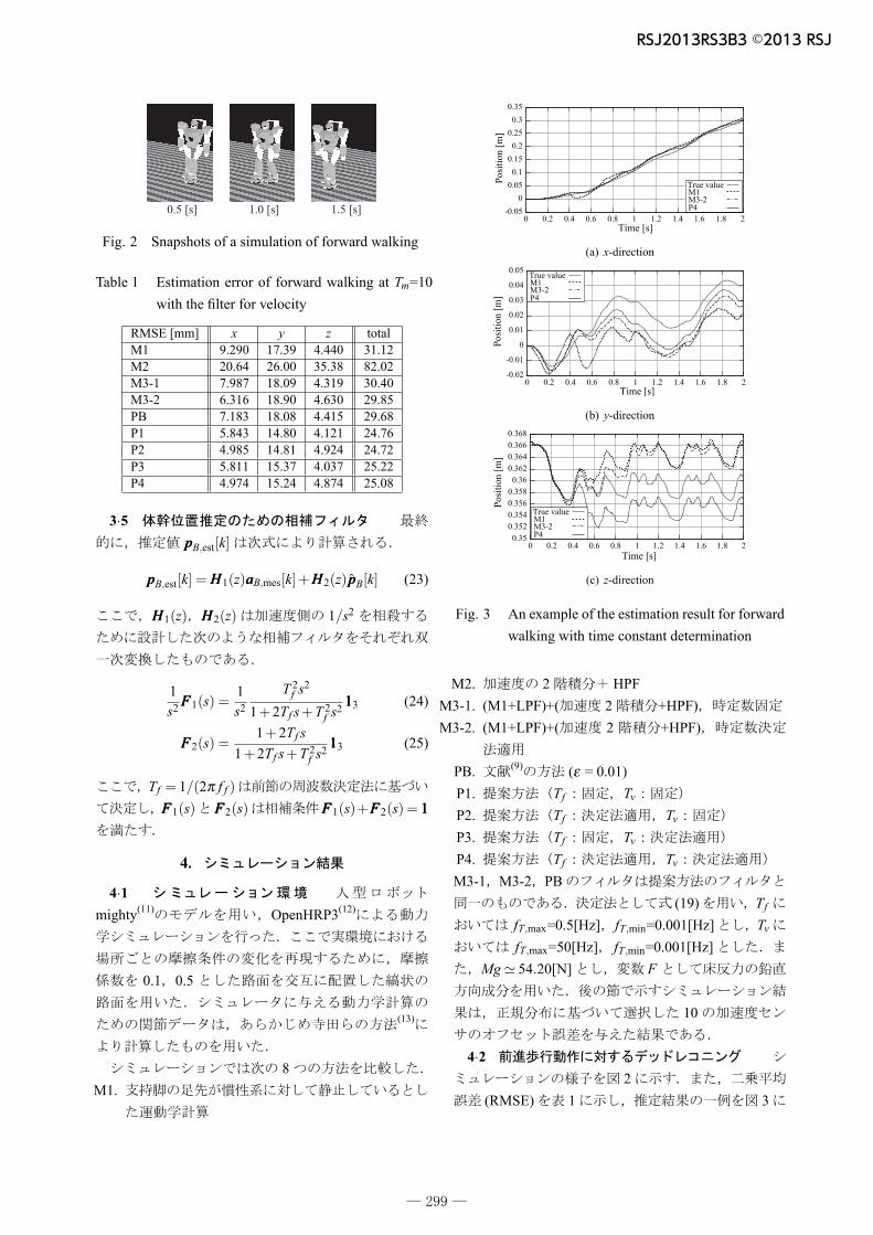
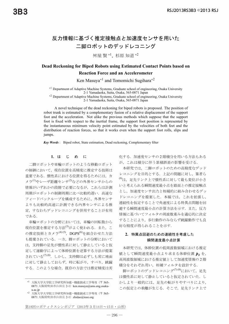
Fig. 2 Snapshots of a simulation of forward walking

Table 1 Estimation error of forward walking at Tm=10with the filter for velocity

RMSE [mm] x y z totalM1 9.290 17.39 4.440 31.12M2 20.64 26.00 35.38 82.02M3-1 7.987 18.09 4.319 30.40M3-2 6.316 18.90 4.630 29.85PB 7.183 18.08 4.415 29.68P1 5.843 14.80 4.121 24.76P2 4.985 14.81 4.924 24.72P3 5.811 15.37 4.037 25.22P4 4.974 15.24 4.874 25.08

3·5pppB,est[k]

pppB,est[k] = HHH1(z)aaaB,mes[k]+HHH2(z) p̂ppB[k] (23)

HHH1(z) HHH2(z) 1/s2

1s2FFF1(s) =

1s2

T 2f s2

1+2Tf s+T 2f s21113 (24)

FFF2(s) =1+2Tf s

1+2Tf s+T 2f s21113 (25)

Tf = 1/(2π f f )FFF1(s) FFF2(s) FFF1(s)+FFF2(s) = 111

4.

4·1mighty(11) OpenHRP3(12)

0.1 0.5

(13)

8M1.

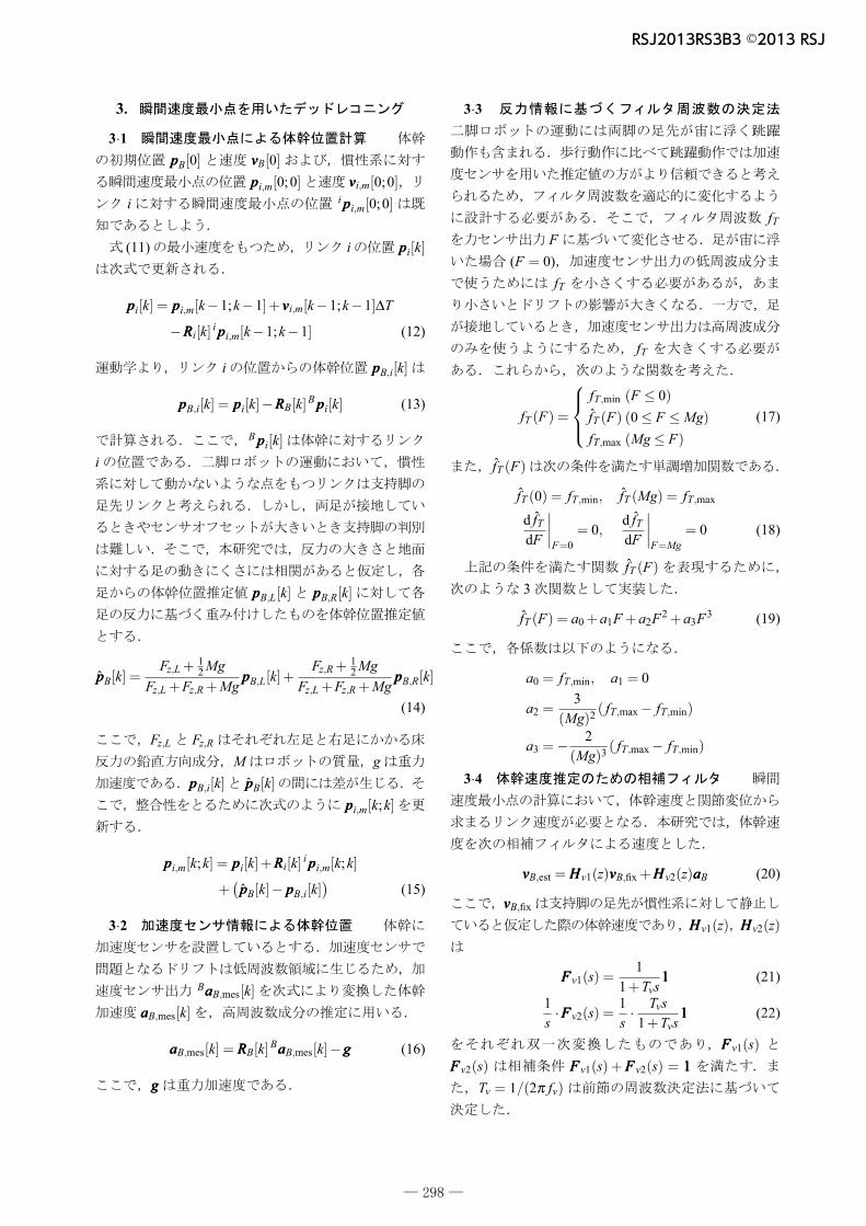
(a) x-direction

(b) y-direction

(c) z-direction

Fig. 3 An example of the estimation result for forwardwalking with time constant determination

M2. 2 HPFM3-1. (M1+LPF)+( 2 +HPF)M3-2. (M1+LPF)+( 2 +HPF)

PB. (9) (ε = 0.01)P1. Tf TvP2. Tf TvP3. Tf TvP4. Tf TvM3-1 M3-2 PB

(19) TffT,max=0.5[Hz] fT,min=0.001[Hz] TvfT,max=50[Hz] fT,min=0.001[Hz]

Mg� 54.20[N] F

10

4·22

(RMSE) 1 3

RSJ2013RS3B3 ©2013 RSJ

― 299 ―

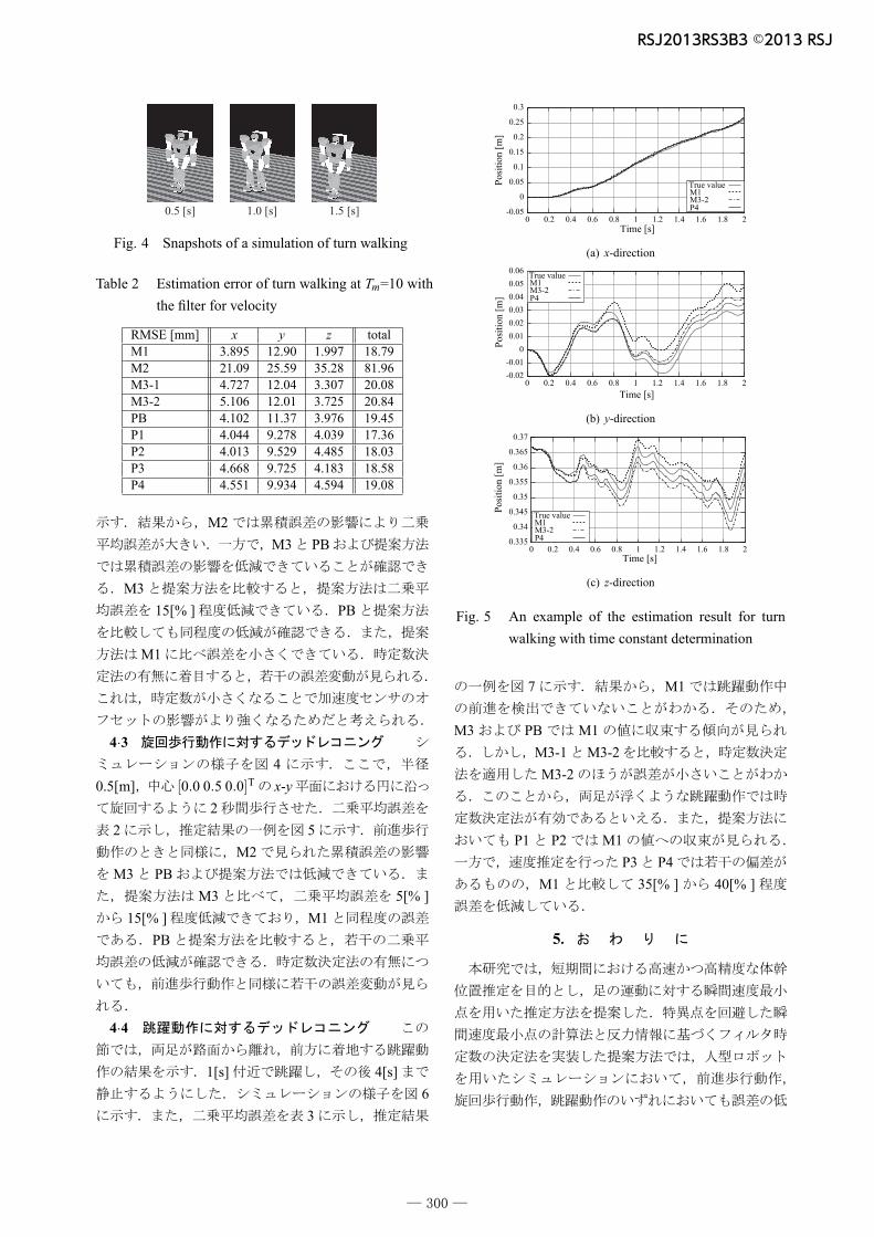
Fig. 4 Snapshots of a simulation of turn walking

Table 2 Estimation error of turn walking at Tm=10 withthe filter for velocity

RMSE [mm] x y z totalM1 3.895 12.90 1.997 18.79M2 21.09 25.59 35.28 81.96M3-1 4.727 12.04 3.307 20.08M3-2 5.106 12.01 3.725 20.84PB 4.102 11.37 3.976 19.45P1 4.044 9.278 4.039 17.36P2 4.013 9.529 4.485 18.03P3 4.668 9.725 4.183 18.58P4 4.551 9.934 4.594 19.08

M2M3 PB

M315[% ] PB

M1

4·34

0.5[m] [0.0 0.5 0.0]T x-y2

2 5M2

M3 PBM3 5[% ]

15[% ] M1PB

4·4

1[s] 4[s]6

3

(a) x-direction

(b) y-direction

(c) z-direction

Fig. 5 An example of the estimation result for turnwalking with time constant determination

7 M1

M3 PB M1M3-1 M3-2M3-2

P1 P2 M1P3 P4

M1 35[% ] 40[% ]

5.

RSJ2013RS3B3 ©2013 RSJ

― 300 ―

Fig. 6 Snapshots of a simulation of jumping

Table 3 Estimation error of jumping at Tm=10 from 0[s]to 4[s] with the filter for velocity

RMSE [mm] x y z totalM1 26.94 0.7441 1.122 28.80M2 93.15 99.40 142.0 334.5M3-1 26.33 2.571 3.745 32.65M3-2 20.48 2.869 3.836 27.19PB 26.00 2.494 3.820 32.31P1 26.96 2.824 4.008 33.79P2 21.15 3.130 4.141 28.42P3 11.43 2.885 5.104 19.42P4 9.056 3.186 5.144 17.39

(A)

( :22680018)

(1) S. Thompson and S. Kagami “Humanoid RobotLocalisation using Stereo Vision”, Proc. of 2005 IEEE-RAS Int. Conf. on Humanoid Robots, pp.19-25, 2005.

(2) “”

17 , (2012), pp.611-617(3) J. L. Crowley, “Asynchronous control of orientation and

displacement in a robot vehicle” Proc. of the 1989 IEEEInt. Conf. on Robotics and Automation, vol.3, (1989),pp.1277-1282.

(4) F. Chenavier, J. L. Crowley, Position Estimation for aMobile Robot Using Vision and Odometry. Proc. of The1992 IEEE Int. Conf. on Robotics and Automation, (1992),pp.2588-2593.

(5) “”

Vol.23 No.3(2005), pp.311-320(6) “DGPS

”20 3A31 (2002)

(7) “”2A1-73-105 (2000)

(a) x-direction

(b) y-direction

(c) z-direction

Fig. 7 An example of the estimation result for jumpingwith time constant determination

(8) “”2A2-M10 (2007)

(9) “” 30

3I1-8 (2012)

(10) K. Masuya, T. Sugihara and M. Yamamoto, “Designof Complementary Filter for High-fidelity AttitudeEstimation based on Sensor Dynamics Compensationwith Decoupled Properties”, Proc. of The 2012 IEEE Int.Conf. on Robotics and Automation, (2012), pp.606-611.

(11) T. Sugihara, K. Yamamoto and Y. Nakamura: “Hardwaredesign of high performance miniature anthropomorphicrobots”, Robotics and Autonomous System, Vol.56, Issue1(2007), pp.82-94.

(12) S. Nakaoka, S. Hattori, F. Kanehiro, S. Kajita and H.Hirukawa: ”Constraint-based Dynamics Simulator forHumanoid Robots with Shock Absorbing Mechanisms,”Proc. of The 2007 IEEE/RSJ Int. Conf. on IntelligentRobots and Systems, (2007), pp.3641-3647.

(13) “

” 25 1G26(2007)

RSJ2013RS3B3 ©2013 RSJ

― 301 ―