s. broverman study guide for the society of …sambroverman.com/sample-mlc09.pdf · s. broverman...
TRANSCRIPT
www.sambroverman.com SOA Exam MLC Study Guide © S. Broverman 2009
S. BROVERMAN STUDY GUIDE
FOR THE
SOCIETY OF ACTUARIESEXAM MLC
2009 EDITION
EXCERPTS
Samuel Broverman, ASA, PHD
copyright © 2008, S. Broverman
www.sambroverman.com SOA Exam MLC Study Guide © S. Broverman 2009
Excerpts:
Table of Contents
Introductory Note
Life Contingencies Section 26 - The Last-Survivor Status and the Common Shock Model
Practice Exam 1 and Solutions
www.sambroverman.com SOA Exam MLC Study Guide © S. Broverman 2009
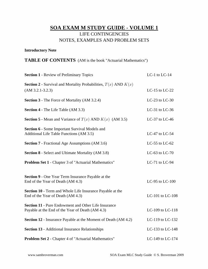
SOA EXAM M STUDY GUIDE - VOLUME 1LIFE CONTINGENCIES
NOTES, EXAMPLES AND PROBLEM SETS
Introductory Note
TABLE OF CONTENTS (AM is the book "Actuarial Mathematics")
Section 1 - Review of Preliminary Topics LC-1 to LC-14
Section 2 - Survival and Mortality Probabilities, AND XÐBÑ OÐBÑ
(AM 3.2.1-3.2.3) LC-15 to LC-22
Section 3 - The Force of Mortality (AM 3.2.4) LC-23 to LC-30
Section 4 - The Life Table (AM 3.3) LC-31 to LC-36
Section 5 - Mean and Variance of AND (AM 3.5) LC-37 to LC-46XÐBÑ OÐBÑ
Section 6 - Some Important Survival Models andAdditional Life Table Functions (AM 3.5) LC-47 to LC-54
Section 7 - Fractional Age Assumptions (AM 3.6) LC-55 to LC-62
Section 8 - Select and Ultimate Mortality (AM 3.8) LC-63 to LC-70
Problem Set 1 - Chapter 3 of "Actuarial Mathematics" LC-71 to LC-94
Section 9 - One Year Term Insurance Payable at theEnd of the Year of Death (AM 4.3) LC-95 to LC-100
Section 10 - Term and Whole Life Insurance Payable at theEnd of the Year of Death (AM 4.3) LC-101 to LC-108
Section 11 - Pure Endowment and Other Life InsurancePayable at the End of the Year of Death (AM 4.3) LC-109 to LC-118
Section 12 - Insurance Payable at the Moment of Death (AM 4.2) LC-119 to LC-132
Section 13 - Additional Insurance Relationships LC-133 to LC-148
Problem Set 2 - Chapter 4 of "Actuarial Mathematics" LC-149 to LC-174
www.sambroverman.com SOA Exam MLC Study Guide © S. Broverman 2009
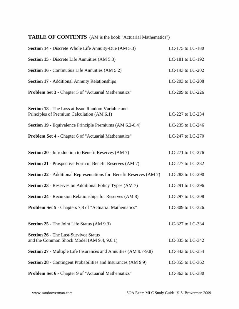
TABLE OF CONTENTS (AM is the book "Actuarial Mathematics")
Section 14 - Discrete Whole Life Annuity-Due (AM 5.3) LC-175 to LC-180
Section 15 - Discrete Life Annuities (AM 5.3) LC-181 to LC-192
Section 16 - Continuous Life Annuities (AM 5.2) LC-193 to LC-202
Section 17 - Additional Annuity Relationships LC-203 to LC-208
Problem Set 3 - Chapter 5 of "Actuarial Mathematics" LC-209 to LC-226
Section 18 - The Loss at Issue Random Variable andPrinciples of Premium Calculation (AM 6.1) LC-227 to LC-234
Section 19 - Equivalence Principle Premiums (AM 6.2-6.4) LC-235 to LC-246
Problem Set 4 - Chapter 6 of "Actuarial Mathematics" LC-247 to LC-270
Section 20 - Introduction to Benefit Reserves (AM 7) LC-271 to LC-276
Section 21 - Prospective Form of Benefit Reserves (AM 7) LC-277 to LC-282
Section 22 - Additional Representations for Benefit Reserves (AM 7) LC-283 to LC-290
Section 23 - Reserves on Additional Policy Types (AM 7) LC-291 to LC-296
Section 24 - Recursion Relationships for Reserves (AM 8) LC-297 to LC-308
Problem Set 5 - Chapters 7,8 of "Actuarial Mathematics" LC-309 to LC-326
Section 25 - The Joint Life Status (AM 9.3) LC-327 to LC-334
Section 26 - The Last-Survivor Statusand the Common Shock Model (AM 9.4, 9.6.1) LC-335 to LC-342
Section 27 - Multiple Life Insurances and Annuities (AM 9.7-9.8) LC-343 to LC-354
Section 28 - Contingent Probabilities and Insurances (AM 9.9) LC-355 to LC-362
Problem Set 6 - Chapter 9 of "Actuarial Mathematics" LC-363 to LC-380
www.sambroverman.com SOA Exam MLC Study Guide © S. Broverman 2009
TABLE OF CONTENTS (AM is the book "Actuarial Mathematics")
Section 29 - Multiple Decrement Models (AM 10) LC-381 to LC-392
Section 30 - Associated Single Decrement Tables (AM 10) LC-393 to LC-406
Section 31 - Valuation of Multiple Decrement Benefits (AM 11) LC-407 to LC-408
Problem Set 7 - Chapters 10-11 of "Actuarial Mathematics" LC-409 to LC-426
Section 32 - Expense Augmented Models (AM 15) LC-427 to LC-444 Problem Set 8 - Chapter 15 of "Actuarial Mathematics" LC-445 to LC-452
ILLUSTRATIVE LIFE TABLE
INDEX OF LIFE CONTINGENCIES TERMINOLOGY AND NOTATION
www.sambroverman.com SOA Exam MLC Study Guide © S. Broverman 2009
SOA EXAM MLC STUDY GUIDE - VOLUME 2POISSON PROCESSES,
MARKOV CHAINS, AND PRACTICE EXAMS
TABLE OF CONTENTS(PM is the "Probability Models" book, and MC is the J. Daniel Study Note)
POISSON PROCESSES (PM is the "Probability Models" book)Notes and Examples (PM 5) PP-1 to PP-14Problem Set - Chapter 5 of PM PP-15 to PP-30
MULTI-STATE TRANSITION MODELS (MARKOV CHAINS) (MC)Notes and Examples MC-1 to MC-16Problem Set MC-17 to MC-34
PRACTICE EXAMSPractice Exam 1 and Solutions PE-1 to PE-20Practice Exam 2 and Solutions PE-21 to PE-40Practice Exam 3 and Solutions PE-41 to PE-60Practice Exam 4 and Solutions PE-61 to PE-78Practice Exam 5 and Solutions PE-79 to PE-102Practice Exam 6 and Solutions PE-103 to PE-124Practice Exam 7 and Solutions PE-125 to PE-142Practice Exam 8 and Solutions PE-143 to PE-166Practice Exam 9 and Solutions PE-167 to PE-188Practice Exam 10 and Solutions PE-189 to PE-210Practice Exam 11 and Solutions PE-211 to PE-232Practice Exam 12 and Solutions PE-233 to PE-254
MAY 2007 SOA EXAM MLC AND SOLUTIONS MLC07-1 to MLC07-22REFERENCE BY TOPIC FOR MAY 2007 EXAM MLC

www.sambroverman.com SOA Exam MLC Study Guide © S. Broverman 2009
INTRODUCTORY NOTE
This study guide is designed to help in the preparation for Exam MLC of the Society ofActuaries (the life contingencies and probability exam).
The material for Exam MLC is divided into one large topic and two smaller topics. The largetopic is life contingencies, and the smaller topics are Poisson processes and multi-state transition(Markov Chain) models. I think that the proper order in which to study the topics is the order inwhich they are listed in the previous sentence.
The study guide is divided into two volumes. Volume 1 consists of review notes, examples andproblem sets for life contingencies. Volume 2 covers the other topics with review notes,examples and problem sets. Volume 2 also contains 12 practice exams of 30 questions eachalong with the May 2007 MLC exam and solutions. There are over 160 examples, over 300problems in the problem sets and 360 questions in the 12 practice exams and May 2007 SOAexam. All of these (about 850) questions have detailed solutions. The notes are broken up intosections (32 sections for life contingencies, and one section each for Poisson Processes andMarkov Chains). Each section has a suggested time frame.
Most of the examples in the notes and almost half of the problems in the problem sets are fromolder SOA or CAS exams (pre-2007) on the relevant topics. The 12 practice exams in Volume 2include many questions from SOA exams released from 2000 to 2006. The practice exams have30 questions each and are designed to be similar to actual 3-hour exams. The SOA and CASquestions are copyrighted by the SOA and CAS, and I gratefully acknowledge that I have beenpermitted to include them in this study guide.
Because of the time constraint on the exam, a crucial aspect of exam taking is the ability to workquickly. I believe that working through many problems and examples is a good way to build upthe speed at which you work. It can also be worthwhile to work through problems that havebeen done before, as this helps to reinforce familiarity, understanding and confidence. Workingmany problems will also help in being able to more quickly identify topic and question types. Ihave attempted, wherever possible, to emphasize shortcuts and efficient and systematic ways ofsetting up solutions. There are also occasional comments on interpretation of the language usedin some exam questions. While the focus of the study guide is on exam preparation, from time totime there will be comments on underlying theory in places that I feel those comments mayprovide useful insight into a topic.
It has been my intention to make this study guide self-contained and comprehensive for all ExamMLC topics, but there are occasional references to the books listed in the SOA exam catalog.While the ability to derive formulas used on the exam is usually not the focus of an examquestion, it is useful in enhancing the understanding of the material and may be helpful inmemorizing formulas. There may be an occasional reference in the review notes to a derivation,but you are encouraged to review the official reference material for more detail on formuladerivations.

www.sambroverman.com SOA Exam MLC Study Guide © S. Broverman 2009
In order for the review notes in this study guide to be most effective, you should have somebackground at the junior or senior college level in probability and statistics. It will be assumedthat you are reasonably familiar with differential and integral calculus.Of the various calculators that are allowed for use on the exam, I think that theBA II PLUS is probably the best choice. It has several memories and has good financialfunctions. I think that the TI-30X IIS would be the second best choice.
There is a set of tables that has been provided with the exam in past sittings. These tables consistof a standard normal distribution probability table and a life table. The tables should beavailable for download from the Society of Actuaries website. It is recommended that you havethem available while studying.
Based on the weight applied to topics on recent actual exams, I have created the practice examsto include about 24 questions on life contingencies and 3 each on Poisson processes and multi-state transition models.
If you have any questions, comments, criticisms or compliments regarding this study guide, youmay contact me at the address below. I apologize in advance for any errors, typographical orotherwise, that you might find, and it would be greatly appreciated if you would bring them tomy attention. I will be maintaining a website for errata that can be accessed fromwww.sambroverman.com . It is my sincere hope that you find this study guide helpful and usefulin your preparation for the exam. I wish you the best of luck on the exam.
Samuel A. Broverman November, 2008Department of StatisticsUniversity of Toronto100 St. George StreetToronto, Ontario CANADA M5S 3G3 E-mail: [email protected] or [email protected]: www.sambroverman.com
www.sambroverman.com SOA Exam MLC Study Guide © S. Broverman 2009
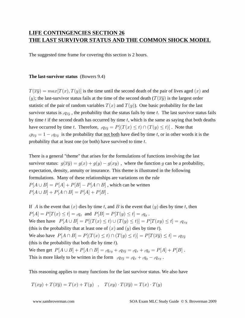
LIFE CONTINGENCIES SECTION 26THE LAST SURVIVOR STATUS AND THE COMMON SHOCK MODEL
The suggested time frame for covering this section is 2 hours.
The last-survivor status (Bowers 9.4)
XÐBCÑ œ 7+BÒX ÐBÑß X ÐCÑÓ ÐBÑ is the time until the second death of the pair of lives aged andÐCÑ X ÐBCÑ; the last-survivor status fails at the time of the second death ( is the largest orderstatistic of the pair of random variables and ). One basic probability for the lastXÐBÑ X ÐCÑ
survivor status is , the probability that the status fails by time . The last survivor status fails> BC; >
by time if the second death has occurred by time , which is the same as saying that both deaths> >
have occurred by time . Therefore, . Note that> ; œ T ÒÐX ÐBÑ Ÿ >Ñ ∩ ÐXÐCÑ Ÿ >ÑÓ> BC
> BC > BC: œ " ; > is the probability that not both have died by time , or in other words it is theprobability that at least one (or both) have survived to time .>
There is a general "theme" that arises for the formulations of functions involving the lastsurvivor status: , where the function can be a probability,1ÐBCÑ œ 1ÐBÑ 1ÐCÑ 1ÐBCÑ 1
expectation, density, annuity or insurance. This theme is illustrated in the followingformulations. Many of these relationships are variations on the ruleT ÒE ∪ FÓ œ T ÒEÓ T ÒFÓ T ÒE ∩ FÓ , which can be writtenT ÒE ∪ FÓ T ÒE ∩ FÓ œ T ÒEÓ T ÒFÓ .
If is the event that dies by time , and is the event that dies by time , thenE ÐBÑ > F ÐCÑ >
T ÒEÓ œ T ÒX ÐBÑ Ÿ >Ó œ ; T ÒFÓ œ T ÒX ÐCÑ Ÿ >Ó œ ;> B > C and .We then have T ÒE ∪ FÓ œ T ÒÐX ÐBÑ Ÿ >Ñ ∪ ÐXÐCÑ Ÿ >ÑÓ œ T ÒX ÐBCÑ Ÿ >Ó œ ;> BC
(this is the probability that at least one of and dies by time ).ÐBÑ ÐCÑ >
We also have T ÒE ∩ FÓ œ T ÒÐX ÐBÑ Ÿ >Ñ ∩ ÐXÐCÑ Ÿ >ÑÓ œ T ÒX ÐBCÑ Ÿ >Ó œ ;> BC
(this is the probability that both die by time ).>
We then get .T ÒE ∪ FÓ T ÒE ∩ FÓ œ ; ; œ ; ; œ T ÒEÓ T ÒFÓ> BC > BC > B > C
This is more likely to be written in the form .> BC > B > C > BC; œ ; ; ;
This reasoning applies to many functions for the last survivor status. We also have
XÐBCÑ XÐBCÑ œ XÐBÑ XÐCÑ ß X ÐBCÑ † X ÐBCÑ œ XÐBÑ † X ÐCÑ
www.sambroverman.com SOA Exam MLC Study Guide © S. Broverman 2009
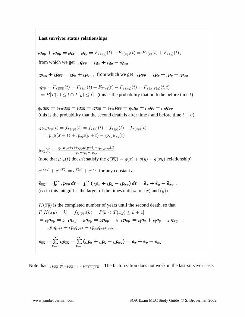
Last survivor status relationships
> BC > BC > B > C; ; œ ; ; œ J Ð>Ñ J Ð>Ñ œ J Ð>Ñ J Ð>ÑXÐBCÑ X ÐBCÑ X ÐBÑ X ÐCÑ ,
from which we get > BC > B > C > BC; œ ; ; ;
, from which we get > BC > BC > B > C > BC > B > C > BC: : œ : : : œ : : :
> BC X ÐBCÑ X ÐBÑ X ÐCÑ X ÐBCÑ X ÐBÑX ÐCÑ; œ J Ð>Ñ œ J Ð>Ñ J Ð>Ñ J Ð>Ñ œ J Ð>ß >Ñ
(this is the probability that both die before time )œ T ÒXÐBÑ Ÿ > ∩ XÐCÑ Ÿ >Ó >
>l? >l? >l? >l?BC >? BC > BC > BC >? BC B C BC; œ ; ; œ : : œ ; ; ;
(this is the probability that the second death is after time and before time )> > ?
> BC BC XÐBCÑ X ÐBÑ X ÐCÑ X ÐBCÑ: Ð>Ñ œ 0 Ð>Ñ œ 0 Ð>Ñ 0 Ð>Ñ 0 Ð>Ñ.
œ : ÐB >Ñ : ÐC >Ñ : Ð>Ñ> B > C > BC BC. . .
.BCÐ>Ñ œ> B > C > BC BC
> B > C > BC
: ÐB>Ñ : ÐC>Ñ : Ð>Ñ: : :
. . .
(note that doesn't satisfy the relationship).BCÐ>Ñ 1ÐBCÑ œ 1ÐBÑ 1ÐCÑ 1ÐBCÑ
for any constant - - œ - - -XÐBCÑ X ÐBCÑ X ÐBÑ X ÐCÑ
./ œ : .> œ Ð : : : Ñ.> œ / / /° ° ° °BC > BC > B > C > BC B C BC! !
∞ ∞' ' ( in this integral is the larger of the times until for and )∞ ÐBÑ ÐCÑ=
is the completed number of years until the second death, so thatOÐBCÑ
T ÒOÐBCÑ œ 5Ó œ 0 Ð5Ñ œ T Ò5 XÐBCÑ Ÿ 5 "ÓOÐBCÑ
œ 5l 5l 5l 5lBC 5" BC 5 BC 5 BC 5" BC B C BC; œ ; ; œ : : œ ; ; ;
œ : ; : ; : ;5 B B5 5 C C5 5 BC B5ÀC5
/ œ : œ Ð : : : Ñ œ / / /BC 5 BC 5 B 5 C 5 BC B C BC5œ" 5œ"
∞ ∞
Note that . The factorization does not work in the last-survivor case.> BC 8 BC >8 B8ÀC8: Á : † :
www.sambroverman.com SOA Exam MLC Study Guide © S. Broverman 2009
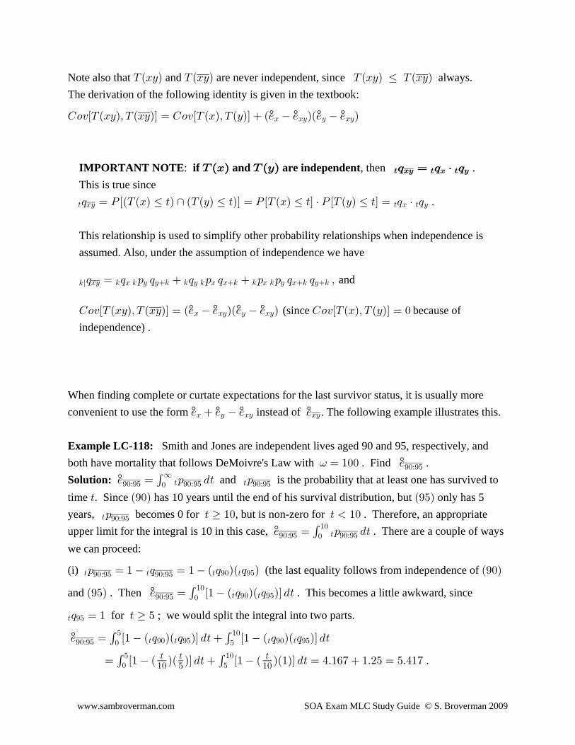
Note also that and are never independent, since always.XÐBCÑ X ÐBCÑ X ÐBCÑ Ÿ XÐBCÑ
The derivation of the following identity is given in the textbook:
G9@ÒX ÐBCÑß X ÐBCÑÓ œ G9@ÒX ÐBÑß X ÐCÑÓ Ð/ / ÑÐ/ / Ñ° ° ° °B BC C BC
IMPORTANT NOTE if and are independent : , then .X ÐBÑ X ÐCÑ ; œ ; † ;> BC > B > C
This is true since
> BC > B > C; œ T ÒÐX ÐBÑ Ÿ >Ñ ∩ ÐXÐCÑ Ÿ >ÑÓ œ T ÒX ÐBÑ Ÿ >Ó † T ÒX ÐCÑ Ÿ >Ó œ ; † ; .
This relationship is used to simplify other probability relationships when independence is assumed. Also, under the assumption of independence we have
and5l BC 5 B 5 C C5 5 C 5 B B5 5 B 5 C B5 C5; œ ; : ; ; : ; : : ; ; ß
(since because of° ° ° °G9@ÒX ÐBCÑß X ÐBCÑÓ œ Ð/ / ÑÐ/ / Ñ G9@ÒX ÐBÑß X ÐCÑÓ œ !B BC C BC
independence) .
When finding complete or curtate expectations for the last survivor status, it is usually moreconvenient to use the form instead of . The following example illustrates this.° ° ° °/ / / /B C BC BC
Example LC-118: Smith and Jones are independent lives aged 90 and 95, respectively, andboth have mortality that follows DeMoivre's Law with . Find .°= œ "!! /*!À*&Solution: and is the probability that at least one has survived to°/ œ : .> :*!À*& *!À*& *!À*&!
∞> >'
time . Since has 10 years until the end of his survival distribution, but only has 5> Ð*!Ñ Ð*&Ñ
years, becomes 0 for , but is non-zero for . Therefore, an appropriate> *!À*&: > "! > "!
upper limit for the integral is 10 in this case, . There are a couple of ways°/ œ : .>*!À*& *!À*&!"!
>'we can proceed:
(i) (the last equality follows from independence of > > > *! > *&*!À*& *!À*&: œ " ; œ " Ð ; ÑÐ ; Ñ Ð*!Ñ
and . Then . This becomes a little awkward, since°Ð*&Ñ / œ Ò" Ð ; ÑÐ ; ÑÓ .>*!À*& !"!
> *! > *&'> *&; œ " > & for ; we would split the integral into two parts.
°/ œ Ò" Ð ; ÑÐ ; ÑÓ .> Ò" Ð ; ÑÐ ; ÑÓ .>*!À*& ! && "!
> *! > *& > *! > *&' ' .œ Ò" Ð ÑÐ ÑÓ .> Ò" Ð ÑÐ"ÑÓ .> œ %Þ"'( "Þ#& œ &Þ%"(' '
! && "!> > >
"! & "!
www.sambroverman.com SOA Exam MLC Study Guide © S. Broverman 2009
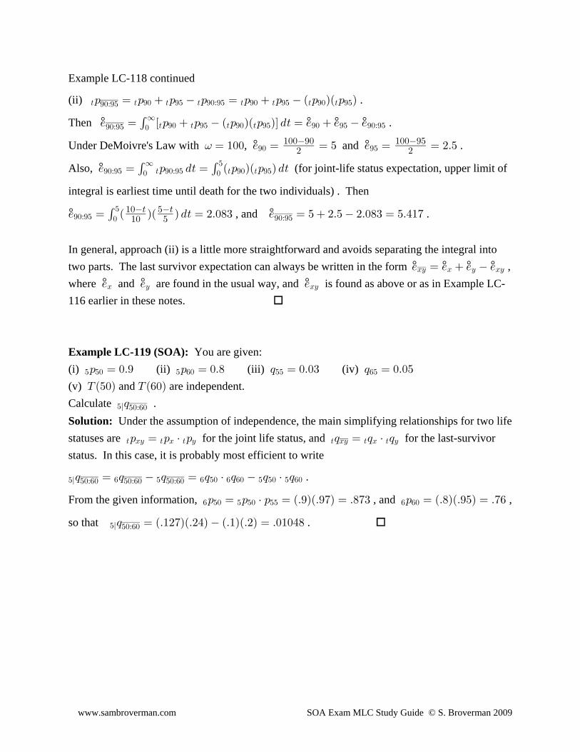
Example LC-118 continued
(ii) .> > *! > *& > *!À*& > *! > *& > *! > *&*!À*&: œ : : : œ : : Ð : ÑÐ : Ñ
Then .° ° ° °/ œ Ò : : Ð : ÑÐ : ÑÓ .> œ / / /*!À*& !∞
> *! > *& > *! > *& *! *& *!À*&'Under DeMoivre's Law with , and .° °= œ "!! / œ œ & / œ œ #Þ&*! *&
"!!*! "!!*&# #
Also, (for joint-life status expectation, upper limit of°/ œ : .> œ Ð : ÑÐ : Ñ .>*!À*& > *!À*& > *! > *&! !∞ &' '
integral is earliest time until death for the two individuals) . Then
/ œ Ð ÑÐ Ñ .> œ #Þ!)$ / œ & #Þ& #Þ!)$ œ &Þ%"(° ° , and .*!À*& !&
*!À*&' "!> &>
"! &
In general, approach (ii) is a little more straightforward and avoids separating the integral intotwo parts. The last survivor expectation can always be written in the form ,° ° ° °/ œ / / /BC B C BC
where and are found in the usual way, and is found as above or as in Example LC-° ° °/ / /B C BC
116 earlier in these notes.
Example LC-119 (SOA): You are given:(i) (ii) (iii) (iv) & &! & '! && '&: œ !Þ* : œ !Þ) ; œ !Þ!$ ; œ !Þ!&
(v) and are independent.XÐ&!Ñ X Ð'!Ñ
Calculate .&l &!À'!;
Solution: Under the assumption of independence, the main simplifying relationships for two lifestatuses are for the joint life status, and for the last-survivor> BC > B > C > BC > B > C: œ : † : ; œ ; † ;
status. In this case, it is probably most efficient to write
&l &!À'! &!À'! &!À'!' & ' &! ' '! & &! & '!; œ ; ; œ ; † ; ; † ; .
From the given information, , and ,' &! & &! && ' '!: œ : † : œ ÐÞ*ÑÐÞ*(Ñ œ Þ)($ : œ ÐÞ)ÑÐÞ*&Ñ œ Þ('
so that . &l &!À'!; œ ÐÞ"#(ÑÐÞ#%Ñ ÐÞ"ÑÐÞ#Ñ œ Þ!"!%)
www.sambroverman.com SOA Exam MLC Study Guide © S. Broverman 2009
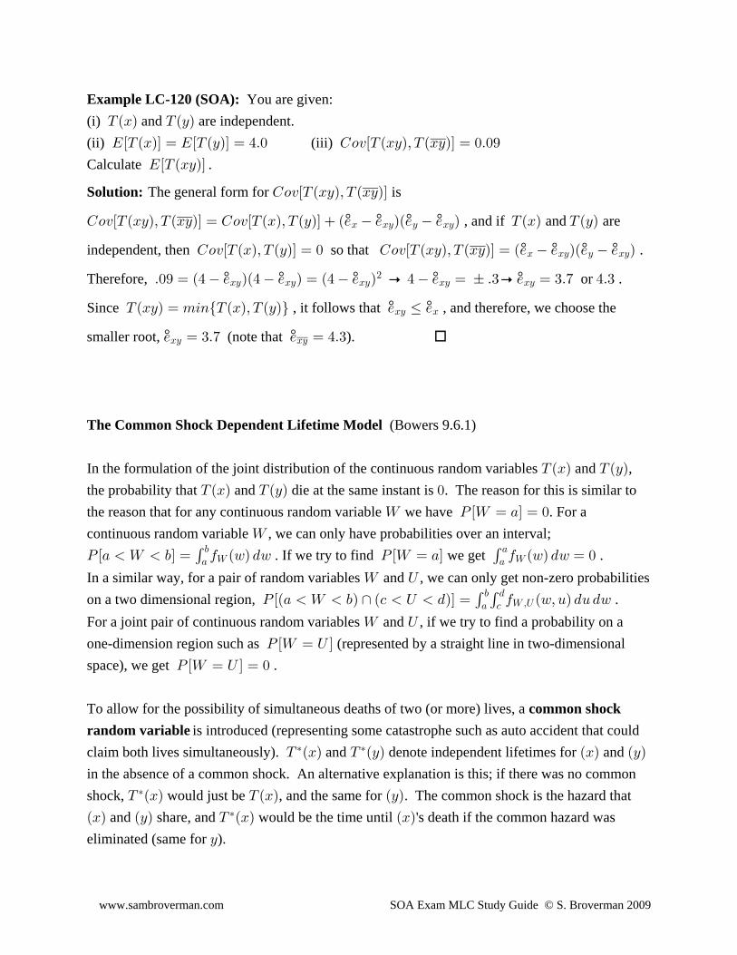
Example LC-120 (SOA): You are given:(i) and are independent.XÐBÑ X ÐCÑ
(ii) (iii) IÒXÐBÑÓ œ IÒXÐCÑÓ œ %Þ! G9@ÒX ÐBCÑß X ÐBCÑÓ œ !Þ!*
Calculate .IÒXÐBCÑÓ
Solution: The general form for isG9@ÒX ÐBCÑß X ÐBCÑÓ
G9@ÒX ÐBCÑß X ÐBCÑÓ œ G9@ÒX ÐBÑß X ÐCÑÓ Ð/ / ÑÐ/ / Ñ XÐBÑ X ÐCÑ° ° ° ° , and if and areB BC C BC
independent, then so that .° ° ° °G9@ÒX ÐBÑß X ÐCÑÓ œ ! G9@ÒX ÐBCÑß X ÐBCÑÓ œ Ð/ / ÑÐ/ / Ñ B BC C BC
Therefore, or .° ° ° ° °Þ!* œ Ð% / ÑÐ% / Ñ œ Ð% / Ñ p % / œ „ Þ$p / œ $Þ( %Þ$BC BC BC BC BC#
Since , it follows that , and therefore, we choose the° °XÐBCÑ œ 738ÖXÐBÑß X ÐCÑ× / Ÿ /BC B
smaller root, (note that ). ° °/ œ $Þ( / œ %Þ$BC BC
The Common Shock Dependent Lifetime Model (Bowers 9.6.1)
In the formulation of the joint distribution of the continuous random variables and ,XÐBÑ X ÐCÑ
the probability that and die at the same instant is . The reason for this is similar toXÐBÑ X ÐCÑ !
the reason that for any continuous random variable we have . For a[ TÒ[ œ +Ó œ !
continuous random variable , we can only have probabilities over an interval;[
TÒ+ [ ,Ó œ 0 ÐAÑ .A T Ò[ œ +Ó 0 ÐAÑ .A œ !' '+ +, +
[ [ . If we try to find we get .In a similar way, for a pair of random variables and , we can only get non-zero probabilities[ Y
on a two dimensional region, .T ÒÐ+ [ ,Ñ ∩ Ð- Y .ÑÓ œ 0 ÐAß ?Ñ .? .A' '+ -, .
[ßY
For a joint pair of continuous random variables and , if we try to find a probability on a[ Y
one-dimension region such as (represented by a straight line in two-dimensionalT Ò[ œ YÓ
space), we get .T Ò[ œ YÓ œ !
To allow for the possibility of simultaneous deaths of two (or more) lives, a common shockrandom variable is introduced (representing some catastrophe such as auto accident that couldclaim both lives simultaneously). and denote independent lifetimes for and X ÐBÑ X ÐCÑ ÐBÑ ÐCч ‡
in the absence of a common shock. An alternative explanation is this; if there was no commonshock, would just be , and the same for . The common shock is the hazard thatX ÐBÑ X ÐBÑ ÐCч
ÐBÑ ÐCÑ X ÐBÑ ÐBÑ and share, and would be the time until 's death if the common hazard was‡
eliminated (same for ).C
www.sambroverman.com SOA Exam MLC Study Guide © S. Broverman 2009
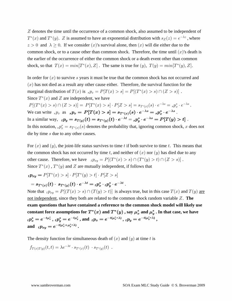
^ denotes the time until the occurrence of a common shock, also assumed to be independent ofX ÐBÑ X ÐCÑ ^ = ÐDÑ œ /‡ ‡ D
^ and . is assumed to have an exponential distribution with , where-
D ! ! ÐBÑ ÐBÑ and . If we consider 's survival alone, then will die either due to the-
common shock, or to a cause other than common shock. Therefore, the time until 's death isÐBÑ
the earlier of the occurrence of either the common shock or a death event other than commonshock, so that . The same is true for , .XÐBÑ œ 738ÒX ÐBÑß ^Ó ÐCÑ X ÐCÑ œ 738ÒX ÐCÑß ^Ó‡ ‡
In order for to survive years it must be true that the common shock has not occurred andÐBÑ =
ÐBÑ has not died as a result any other cause either. Therefore, the survival function for themarginal distribution of is .XÐBÑ : œ T ÒX ÐBÑ =Ó œ T ÒÐX ÐBÑ =Ñ ∩ Ð^ =ÑÓ= B
‡
Since and are independent, we haveX ÐBÑ ^‡
T ÒÐX ÐBÑ =Ñ ∩ Ð^ =ÑÓ œ T ÒX ÐBÑ =Ó † T Ò^ =Ó œ = Ð=Ñ † / œ : † /‡ ‡ = ‡ =X ÐBÑ = B‡
- - .We can write as .= B: = B =X ÐBÑ
= ‡ =B: œ T ÒX ÐBÑ =Ó œ = Ð=Ñ † / œ : † /‡
- -
In a similar way, . > C =X ÐCÑ X ÐCÑ > ‡ =
C: œ = Ð>Ñ œ = Ð>Ñ † / : † / œ T ÒX ÐCÑ >Ó‡- -œ
In this notation, denotes the probability that, ignoring common shock, does not= B‡
X ÐBÑ: œ = Ð=Ñ B‡
die by time due to any other causes.=
For and , the joint-life status survives to time if both survive to time . This means thatÐBÑ ÐCÑ > >
the common shock has not occurred by time , and neither of nor has died due to any> ÐBÑ ÐCÑ
other cause. Therefore, we have . > BC‡ ‡: œ T ÒÐX ÐBÑ =Ñ ∩ ÐX ÐCÑ >Ñ ∩ Ð^ =ÑÓ
Since , and are mutually independent, if follows thatX ÐBÑ X ÐCÑ ^‡ ‡
> BC: œ T ÒX ÐBÑ =Ó † T ÒX ÐCÑ >Ó † T Ò^ =Ó‡ ‡
.œ = Ð>Ñ † = Ð>Ñ † / œ : † : † /X ÐBÑ X ÐCÑ > ‡ ‡ >
> >B C‡ ‡ - -
Note that is always true, but in this case and > BC: œ T ÒÐX ÐBÑ =Ñ ∩ ÐXÐCÑ >ÑÓ X ÐBÑ X ÐCÑ arenot independent, since they both are related to the common shock random variable . ^ Theexam questions that have contained a reference to the common shock model will likely useconstant force assumptions for and , say and . In that case, we haveX ÐBÑ X ÐCч ‡ ‡ ‡
B C . .
> > > B > CB C‡ > ‡ >> >: œ / ß : œ / : œ / ß : œ /. . -. . -‡ ‡
B B‡ ‡C C , and ,( + ) ( + )
and .> BC> : œ / ( + ). . -‡ ‡
B C
The density function for simultaneous death of and at time isÐBÑ ÐCÑ >
.0 Ð>ß >Ñ œ / † = Ð>Ñ † = Ð>ÑXÐBÑX ÐCÑ X ÐBÑ X ÐCÑ >- -
‡ ‡
www.sambroverman.com SOA Exam MLC Study Guide © S. Broverman 2009
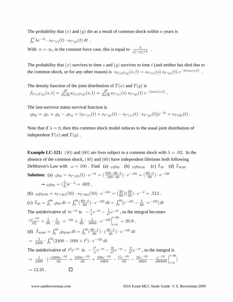
The probability that and die as a result of common shock within years isÐBÑ ÐCÑ 8
'!8 >
X ÐBÑ X ÐCÑ-/ † = Ð>Ñ † = Ð>Ñ .>-‡ ‡ .
With , in the constant force case, this is equal to .8 œ ∞ -. . -‡ ‡B C +
The probability that survives to time and survives to time (and neither has died due toÐBÑ = ÐCÑ >
the common shock, or for any other reason) is .= Ð=ß >Ñ œ = Ð=Ñ = Ð>Ñ /XÐBÑX ÐCÑ X ÐBÑ X ÐCÑ Ò7+BÐ=ß>ÑÓ
‡ ‡-
The density function of the joint distribution of and isXÐBÑ X ÐCÑ
.0 Ð=ß >Ñ œ = Ð=ß >Ñ œ = Ð=Ñ = Ð>Ñ /XÐBÑX ÐCÑ X ÐBÑX ÐCÑ X ÐBÑ X ÐCÑ Ò7+BÐ=ß>ÑÓ` `
`= `> `= `>
# #
‡ ‡-
The last-survivor status survival function is .> BC > B > C > BC X ÐBÑ X ÐCÑ X ÐBÑ X ÐCÑ X ÐBCÑ
>: œ : : : œ Ò= Ð>Ñ = Ð>Ñ = Ð>Ñ † = Ð>ÑÓ/ œ = Ð>ч ‡ ‡ ‡-
Note that if , then this common shock model reduces to the usual joint distribution of- œ !
independent and .XÐBÑ X ÐCÑ
Example LC-121: and are lives subject to a common shock with . In theÐ%!Ñ Ð'!Ñ œ Þ!#-
absence of the common shock, and have independent lifetimes both followingÐ%!Ñ Ð'!Ñ
DeMoivre's Law with . Find (a) (b) (c) (d) ° ° = œ "!! : : / /"! %! "! %!À'! %! %!À'!
Solution: (a) > %! X Ð%!Ñ > Þ!#> Þ!#>: œ = Ð>Ñ † / œ Ð Ñ † / œ Ð Ñ † /‡- "!!%!> '!>
"!!%! '!
.p : œ Ð Ñ/ œ Þ')#"! %!Þ#&
'
(b) ."! %!À'! X Ð%!Ñ X Ð'!Ñ"! Þ#: œ = Ð"!Ñ † = Ð"!Ñ † / œ Ð ÑÐ Ñ † / œ Þ&"#‡ ‡
- &! $!'! %!
(c) °/ œ : .> œ Ð Ñ † / .> œ Ò/ † / Ó .>%! > %!! ! !'! '! '!Þ!#> Þ!#> Þ!#>' ' ''!> >
'! '!
The antiderivative of is , so the integral becomes>/ / /+> +> +>> "+ +#
/ " > " "Þ!# '! Þ!# '! Þ!!!%
Þ!#>
† † / † † / œ #!Þ*Þ!#> Þ!#>
>œ!
>œ'!¹ .
(d) °/ œ : .> œ Ð Ñ † Ð Ñ † / .>%!À'! > %!À'!! !'! %! Þ!#>' ' '!> %!>
'! %!
œ † Ð#%!! "!!> > Ñ † / .> "#%!!
'!%! # Þ!#>
The antiderivative of is , so the integral is> / / / /# +> +> +> +>> #> #+ + +
#
# $
œ † Ò Ó " #%!!/ "!!>/ "!!/ > / #>/ /#%!! Þ!# Þ!# Þ!!!% Þ!# Þ!!!% Þ!!!!!)
Þ!#> Þ!#> Þ!#> # Þ!#> Þ!#> Þ!#> ¹>œ!
>œ'!
œ "#Þ$& .
www.sambroverman.com SOA Exam MLC Study Guide © S. Broverman 2009
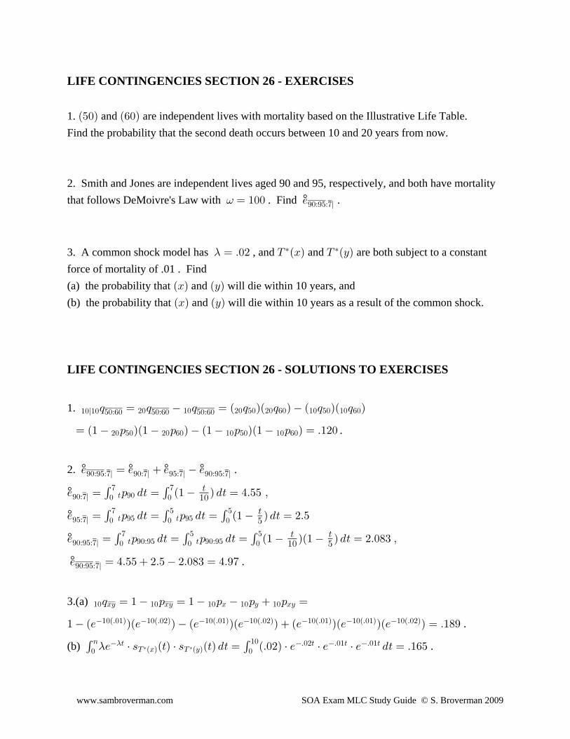
LIFE CONTINGENCIES SECTION 26 - EXERCISES
1. and are independent lives with mortality based on the Illustrative Life Table.Ð&!Ñ Ð'!Ñ
Find the probability that the second death occurs between 10 and 20 years from now.
2. Smith and Jones are independent lives aged 90 and 95, respectively, and both have mortalitythat follows DeMoivre's Law with . Find .°= œ "!! /*!À*&À(l
3. A common shock model has , and and are both subject to a constant- œ Þ!# X ÐBÑ X ÐCч ‡
force of mortality of .01 . Find(a) the probability that and will die within 10 years, andÐBÑ ÐCÑ
(b) the probability that and will die within 10 years as a result of the common shock.ÐBÑ ÐCÑ
LIFE CONTINGENCIES SECTION 26 - SOLUTIONS TO EXERCISES
1. "!l"! &!À'! &!À'! &!À'!#! "! #! &! #! '! "! &! "! '!; œ ; ; œ Ð ; ÑÐ ; Ñ Ð ; ÑÐ ; Ñ
œ Ð" : ÑÐ" : Ñ Ð" : ÑÐ" : Ñ œ Þ"#!#! &! #! '! "! &! "! '! .
2. .° ° ° °/ œ / / /*!À*&À(l *!À(l *&À(l *!À*&À(l
/ œ : .> œ Ð" Ñ .> œ %Þ&& ß°*!À(l ! !
( (> *!' ' >
"!
/ œ : .> œ : .> œ Ð" Ñ .> œ #Þ&°*&À(l ! ! !
( & &> *& > *&' ' ' >
&
/ œ : .> œ : .> œ Ð" ÑÐ" Ñ .> œ #Þ!)$ ß° *!À*&À(l ! ! !( & &> *!À*& > *!À*&' ' ' > >
"! &
.°/ œ %Þ&& #Þ& #Þ!)$ œ %Þ*(*!À*&À(l
3.(a) "! BC "! BC "! B "! C "! BC; œ " : œ " : : : œ
" Ð/ ÑÐ/ Ñ Ð/ ÑÐ/ Ñ Ð/ ÑÐ/ ÑÐ/ Ñ œ Þ")*"!ÐÞ!"Ñ "!ÐÞ!#Ñ "!ÐÞ!"Ñ "!ÐÞ!#Ñ "!ÐÞ!"Ñ "!ÐÞ!"Ñ "!ÐÞ!#Ñ .
(b) .' '! !8 "! > Þ!#> Þ!"> Þ!">
X ÐBÑ X ÐCÑ-/ † = Ð>Ñ † = Ð>Ñ .> œ ÐÞ!#Ñ † / † / † / .> œ Þ"'&-‡ ‡
www.sambroverman.com SOA Exam MLC Study Guide © S. Broverman 2009
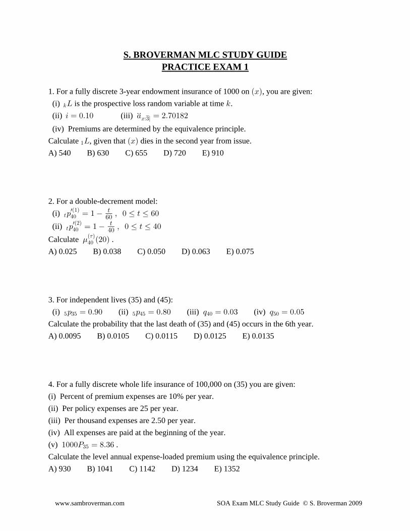
S. BROVERMAN MLC STUDY GUIDEPRACTICE EXAM 1
1. For a fully discrete 3-year endowment insurance of 1000 on , you are given:ÐBÑ
(i) is the prospective loss random variable at time .5P 5
(ii) (iii) 3 œ !Þ"! + œ #Þ(!")#ÞÞBÀ$l
(iv) Premiums are determined by the equivalence principle.Calculate , given that dies in the second year from issue."P ÐBÑ
A) 540 B) 630 C) 655 D) 720 E) 910
2. For a double-decrement model: (i) > %!
wÐ"Ñ: œ " ß ! Ÿ > Ÿ '!>
'!
(ii) > %!wÐ#Ñ
: œ " ß ! Ÿ > Ÿ %!>%!
Calculate ..%!Ð Ñ7
Ð#!Ñ
A) 0.025 B) 0.038 C) 0.050 D) 0.063 E) 0.075
3. For independent lives (35) and (45): (i) (ii) (iii) (iv) & $& & %& %! &!: œ !Þ*! : œ !Þ)! ; œ !Þ!$ ; œ !Þ!&
Calculate the probability that the last death of (35) and (45) occurs in the 6th year.A) 0.0095 B) 0.0105 C) 0.0115 D) 0.0125 E) 0.0135
4. For a fully discrete whole life insurance of 100,000 on (35) you are given:(i) Percent of premium expenses are 10% per year.(ii) Per policy expenses are 25 per year.(iii) Per thousand expenses are 2.50 per year.(iv) All expenses are paid at the beginning of the year.(v) ."!!!T œ )Þ$'$&
Calculate the level annual expense-loaded premium using the equivalence principle.A) 930 B) 1041 C) 1142 D) 1234 E) 1352
www.sambroverman.com SOA Exam MLC Study Guide © S. Broverman 2009
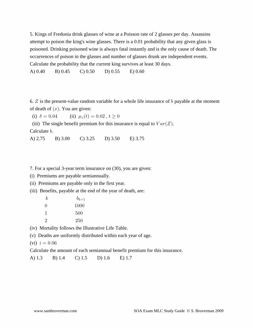
5. Kings of Fredonia drink glasses of wine at a Poisson rate of 2 glasses per day. Assassinsattempt to poison the king's wine glasses. There is a 0.01 probability that any given glass ispoisoned. Drinking poisoned wine is always fatal instantly and is the only cause of death. Theoccurrences of poison in the glasses and number of glasses drunk are independent events.Calculate the probability that the current king survives at least 30 days.A) 0.40 B) 0.45 C) 0.50 D) 0.55 E) 0.60
6. is the present-value random variable for a whole life insurance of payable at the moment^ ,
of death of . You are given:ÐBÑ
(i) (ii) $ .œ !Þ!% Ð>Ñ œ !Þ!# ß > !B
(iii) The single benefit premium for this insurance is equal to .Z +<Ð^Ñ
Calculate .,A) 2.75 B) 3.00 C) 3.25 D) 3.50 E) 3.75
7. For a special 3-year term insurance on (30), you are given:(i) Premiums are payable semiannually.(ii) Premiums are payable only in the first year.(iii) Benefits, payable at the end of the year of death, are: 5 ,5"
! "!!!
" &!!
# #&!
(iv) Mortality follows the Illustrative Life Table.(v) Deaths are uniformly distributed within each year of age.(vi) 3 œ !Þ!'
Calculate the amount of each semiannual benefit premium for this insurance.A) 1.3 B) 1.4 C) 1.5 D) 1.6 E) 1.7
www.sambroverman.com SOA Exam MLC Study Guide © S. Broverman 2009
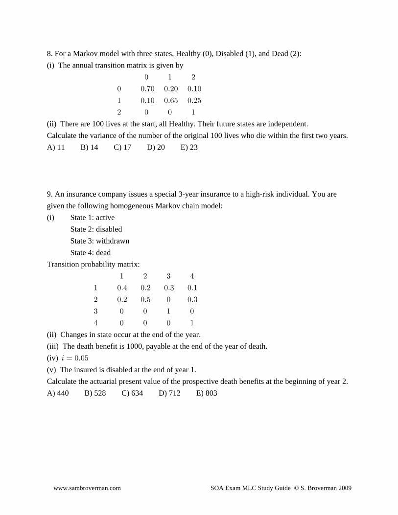
8. For a Markov model with three states, Healthy (0), Disabled (1), and Dead (2):(i) The annual transition matrix is given by ! " #
! !Þ(! !Þ#! !Þ"!
" !Þ"! !Þ'& !Þ#&
# ! ! "
(ii) There are 100 lives at the start, all Healthy. Their future states are independent.Calculate the variance of the number of the original 100 lives who die within the first two years.A) 11 B) 14 C) 17 D) 20 E) 23
9. An insurance company issues a special 3-year insurance to a high-risk individual. You aregiven the following homogeneous Markov chain model:(i) State 1: active State 2: disabled State 3: withdrawn State 4: deadTransition probability matrix: " # $ %
" !Þ% !Þ# !Þ$ !Þ"
# !Þ# !Þ& ! !Þ$
$ ! ! " !
% ! ! ! "
(ii) Changes in state occur at the end of the year.(iii) The death benefit is 1000, payable at the end of the year of death.(iv) 3 œ !Þ!&
(v) The insured is disabled at the end of year 1.Calculate the actuarial present value of the prospective death benefits at the beginning of year 2.A) 440 B) 528 C) 634 D) 712 E) 803
www.sambroverman.com SOA Exam MLC Study Guide © S. Broverman 2009
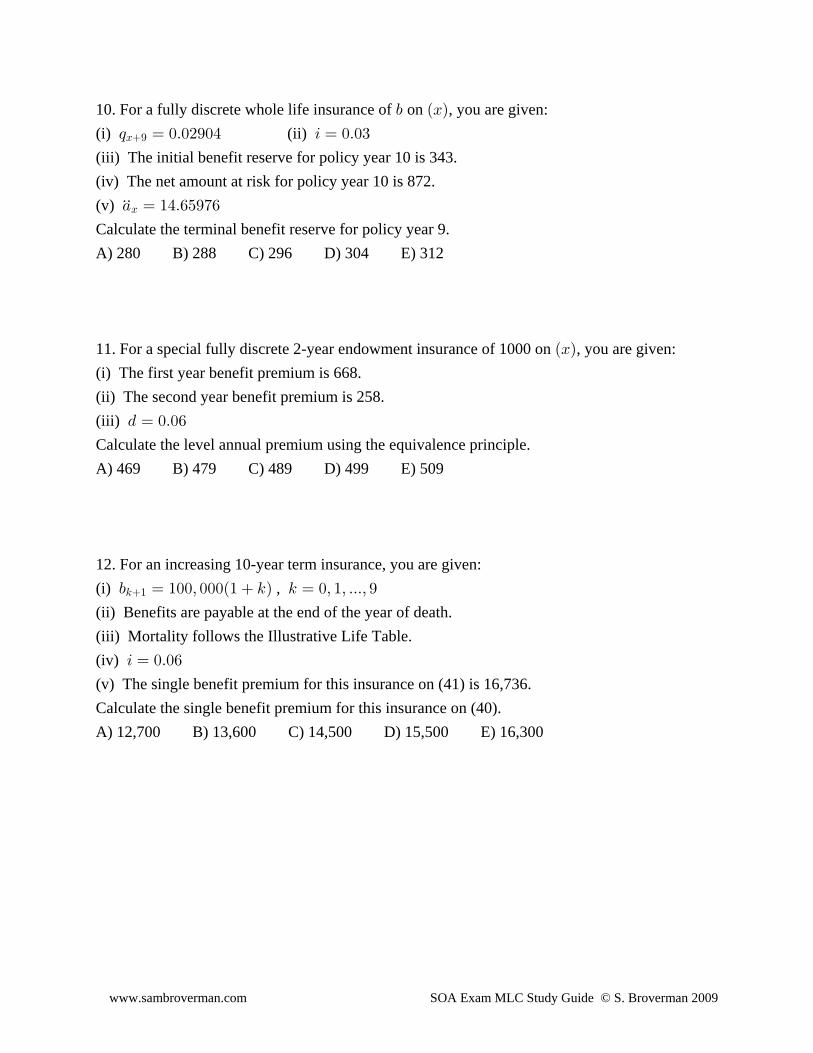
10. For a fully discrete whole life insurance of on , you are given:, ÐBÑ
(i) (ii) ; œ !Þ!#*!% 3 œ !Þ!$B*
(iii) The initial benefit reserve for policy year 10 is 343.(iv) The net amount at risk for policy year 10 is 872.(v) + œ "%Þ'&*('
ÞÞB
Calculate the terminal benefit reserve for policy year 9.A) 280 B) 288 C) 296 D) 304 E) 312
11. For a special fully discrete 2-year endowment insurance of 1000 on , you are given:ÐBÑ
(i) The first year benefit premium is 668.(ii) The second year benefit premium is 258.(iii) . œ !Þ!'
Calculate the level annual premium using the equivalence principle.A) 469 B) 479 C) 489 D) 499 E) 509
12. For an increasing 10-year term insurance, you are given:(i) , , œ "!!ß !!!Ð" 5Ñ 5 œ !ß "ß ÞÞÞß *5"
(ii) Benefits are payable at the end of the year of death.(iii) Mortality follows the Illustrative Life Table.(iv) 3 œ !Þ!'
(v) The single benefit premium for this insurance on (41) is 16,736.Calculate the single benefit premium for this insurance on (40).A) 12,700 B) 13,600 C) 14,500 D) 15,500 E) 16,300
www.sambroverman.com SOA Exam MLC Study Guide © S. Broverman 2009
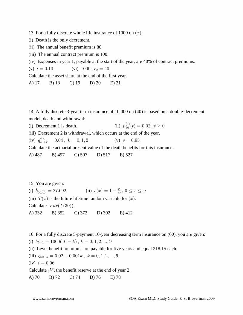
13. For a fully discrete whole life insurance of 1000 on :ÐBÑ
(i) Death is the only decrement.(ii) The annual benefit premium is 80.(iii) The annual contract premium is 100.(iv) Expenses in year 1, payable at the start of the year, are 40% of contract premiums.(v) (vi) 3 œ !Þ"! "!!! Z œ %!" B
Calculate the asset share at the end of the first year.A) 17 B) 18 C) 19 D) 20 E) 21
14. A fully discrete 3-year term insurance of 10,000 on (40) is based on a double-decrementmodel, death and withdrawal:(i) Decrement 1 is death. (ii) .%!
Ð"ÑÐ>Ñ œ !Þ!# ß > !
(iii) Decrement 2 is withdrawal, which occurs at the end of the year.(iv) , (v) ; œ !Þ!% 5 œ !ß "ß # @ œ !Þ*&%!5
wÐ#Ñ
Calculate the actuarial present value of the death benefits for this insurance.A) 487 B) 497 C) 507 D) 517 E) 527
15. You are given:(i) (ii) °/ œ #(Þ'*# =ÐBÑ œ " ß ! Ÿ B Ÿ$!À%!l
B= =
(iii) is the future lifetime random variable for .XÐBÑ ÐBÑ
Calculate .Z +<ÐX Ð$!ÑÑ
A) 332 B) 352 C) 372 D) 392 E) 412
16. For a fully discrete 5-payment 10-year decreasing term insurance on (60), you are given:(i) , œ "!!!Ð"! 5Ñ ß 5 œ !ß "ß #ß ÞÞÞß *5"
(ii) Level benefit premiums are payable for five years and equal 218.15 each.(iii) ; œ !Þ!# !Þ!!"5 ß 5 œ !ß "ß #ß ÞÞÞß *'!5
(iv) 3 œ !Þ!'
Calculate , the benefit reserve at the end of year 2.#Z
A) 70 B) 72 C) 74 D) 76 E) 78
www.sambroverman.com SOA Exam MLC Study Guide © S. Broverman 2009
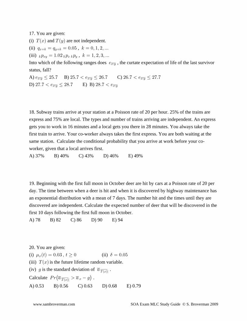
17. You are given:(i) and are not independent.XÐBÑ X ÐCÑ
(ii) , ; œ ; œ !Þ!& 5 œ !ß "ß #ß ÞÞÞB5 C5
(iii) , 5 BC 5 B 5 C: œ "Þ!# : : 5 œ "ß #ß $ß ÞÞÞ
Into which of the following ranges does , the curtate expectation of life of the last survivor/BÀC
status, fall?A) B) C) / Ÿ #&Þ( #&Þ( / Ÿ #'Þ( #'Þ( / Ÿ #(Þ(BÀC BÀC BÀC
D) E) B) #(Þ( / Ÿ #)Þ( #)Þ( /BÀC BÀC
18. Subway trains arrive at your station at a Poisson rate of 20 per hour. 25% of the trains areexpress and 75% are local. The types and number of trains arriving are independent. An expressgets you to work in 16 minutes and a local gets you there in 28 minutes. You always take thefirst train to arrive. Your co-worker always takes the first express. You are both waiting at thesame station. Calculate the conditional probability that you arrive at work before your co-worker, given that a local arrives first.A) 37% B) 40% C) 43% D) 46% E) 49%
19. Beginning with the first full moon in October deer are hit by cars at a Poisson rate of 20 perday. The time between when a deer is hit and when it is discovered by highway maintenance hasan exponential distribution with a mean of 7 days. The number hit and the times until they arediscovered are independent. Calculate the expected number of deer that will be discovered in thefirst 10 days following the first full moon in October.A) 78 B) 82 C) 86 D) 90 E) 94
20. You are given:(i) (ii) . $BÐ>Ñ œ !Þ!$ ß > ! œ !Þ!&
(iii) is the future lifetime random variable. XÐBÑ
(iv) is the standard deviation of .1 +XÐBÑl
Calculate .T< + + 1 ˆ ‰XÐBÑl B
A) 0.53 B) 0.56 C) 0.63 D) 0.68 E) 0.79
www.sambroverman.com SOA Exam MLC Study Guide © S. Broverman 2009
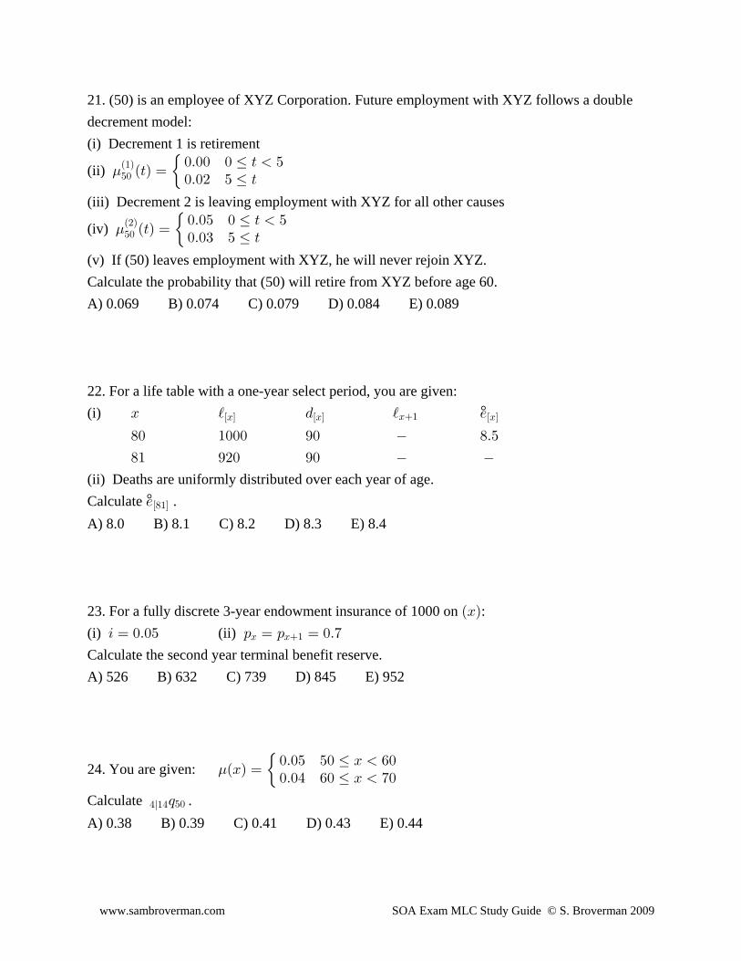
21. (50) is an employee of XYZ Corporation. Future employment with XYZ follows a doubledecrement model:(i) Decrement 1 is retirement
(ii) .&!Ð"Ñ
Ð>Ñ œ!Þ!! ! Ÿ > &!Þ!# & Ÿ >œ
(iii) Decrement 2 is leaving employment with XYZ for all other causes
(iv) .&!Ð#Ñ
Ð>Ñ œ!Þ!& ! Ÿ > &!Þ!$ & Ÿ >œ
(v) If (50) leaves employment with XYZ, he will never rejoin XYZ.Calculate the probability that (50) will retire from XYZ before age 60.A) 0.069 B) 0.074 C) 0.079 D) 0.084 E) 0.089
22. For a life table with a one-year select period, you are given:(i) °B j . j /ÒBÓ ÒBÓ ÒBÓB"
)! "!!! *! )Þ&
)" *#! *!
(ii) Deaths are uniformly distributed over each year of age.Calculate .°/Ò)"ÓA) 8.0 B) 8.1 C) 8.2 D) 8.3 E) 8.4
23. For a fully discrete 3-year endowment insurance of 1000 on :ÐBÑ
(i) (ii) 3 œ !Þ!& : œ : œ !Þ(B B"
Calculate the second year terminal benefit reserve.A) 526 B) 632 C) 739 D) 845 E) 952
24. You are given: .ÐBÑ œ!Þ!& &! Ÿ B '!!Þ!% '! Ÿ B (!œ
Calculate .%l"% &!;
A) 0.38 B) 0.39 C) 0.41 D) 0.43 E) 0.44
www.sambroverman.com SOA Exam MLC Study Guide © S. Broverman 2009
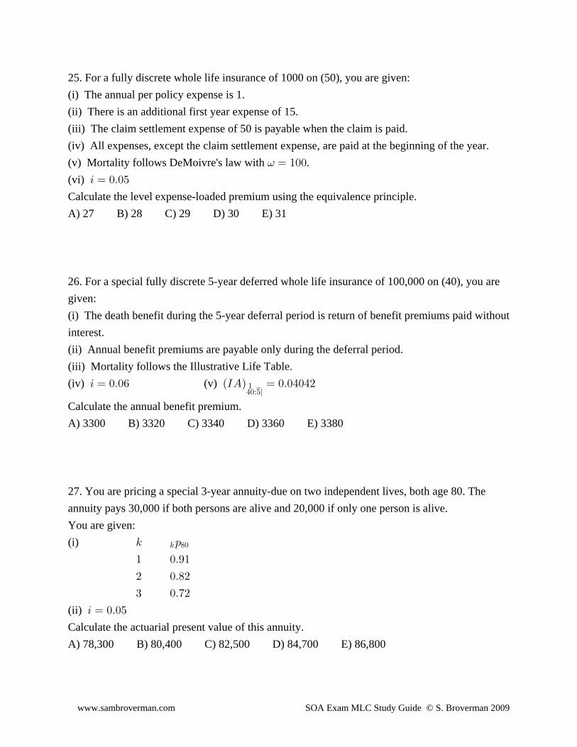
25. For a fully discrete whole life insurance of 1000 on (50), you are given:(i) The annual per policy expense is 1.(ii) There is an additional first year expense of 15.(iii) The claim settlement expense of 50 is payable when the claim is paid.(iv) All expenses, except the claim settlement expense, are paid at the beginning of the year.(v) Mortality follows DeMoivre's law with .= œ "!!
(vi) 3 œ !Þ!&
Calculate the level expense-loaded premium using the equivalence principle.A) 27 B) 28 C) 29 D) 30 E) 31
26. For a special fully discrete 5-year deferred whole life insurance of 100,000 on (40), you aregiven:(i) The death benefit during the 5-year deferral period is return of benefit premiums paid withoutinterest.(ii) Annual benefit premiums are payable only during the deferral period.(iii) Mortality follows the Illustrative Life Table.(iv) (v) 3 œ !Þ!' ÐMEÑ œ !Þ!%!%#
%!À&l"
Calculate the annual benefit premium.A) 3300 B) 3320 C) 3340 D) 3360 E) 3380
27. You are pricing a special 3-year annuity-due on two independent lives, both age 80. Theannuity pays 30,000 if both persons are alive and 20,000 if only one person is alive.You are given:(i) 5 :5 )!
" !Þ*"
# !Þ)#
$ !Þ(#
(ii) 3 œ !Þ!&
Calculate the actuarial present value of this annuity.A) 78,300 B) 80,400 C) 82,500 D) 84,700 E) 86,800
www.sambroverman.com SOA Exam MLC Study Guide © S. Broverman 2009
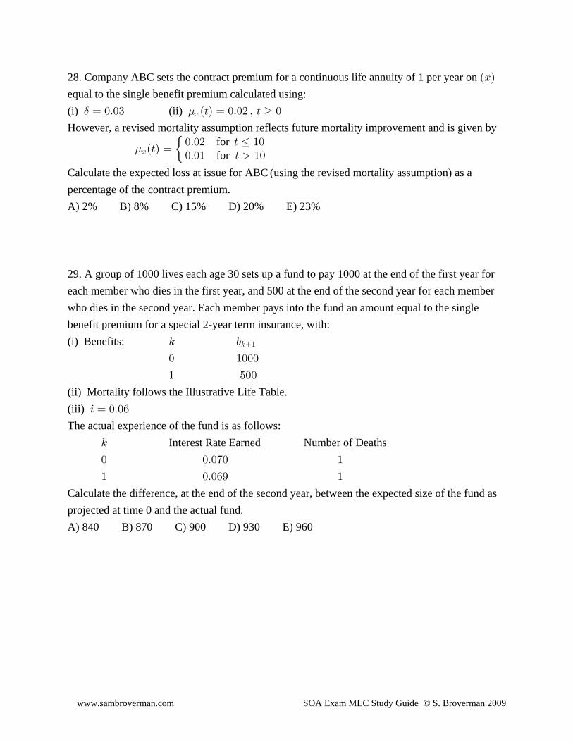
28. Company ABC sets the contract premium for a continuous life annuity of 1 per year on ÐBÑequal to the single benefit premium calculated using:(i) (ii) $ .œ !Þ!$ Ð>Ñ œ !Þ!# ß > !B
However, a revised mortality assumption reflects future mortality improvement and is given by
for for .BÐ>Ñ œ
!Þ!# > Ÿ "!!Þ!" > "!œ
Calculate the expected loss at issue for ABC (using the revised mortality assumption) as apercentage of the contract premium.A) 2% B) 8% C) 15% D) 20% E) 23%
29. A group of 1000 lives each age 30 sets up a fund to pay 1000 at the end of the first year foreach member who dies in the first year, and 500 at the end of the second year for each memberwho dies in the second year. Each member pays into the fund an amount equal to the singlebenefit premium for a special 2-year term insurance, with:(i) Benefits: 5 ,5"
! "!!!
" &!!
(ii) Mortality follows the Illustrative Life Table.(iii) 3 œ !Þ!'
The actual experience of the fund is as follows: Interest Rate Earned Number of Deaths5
! !Þ!(! "
" !Þ!'* "
Calculate the difference, at the end of the second year, between the expected size of the fund asprojected at time 0 and the actual fund.A) 840 B) 870 C) 900 D) 930 E) 960
www.sambroverman.com SOA Exam MLC Study Guide © S. Broverman 2009
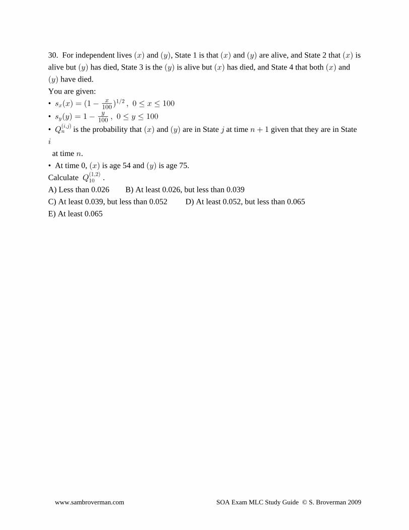
30. For independent lives and , State 1 is that and are alive, and State 2 that isÐBÑ ÐCÑ ÐBÑ ÐCÑ ÐBÑ
alive but has died, State 3 is the is alive but has died, and State 4 that both andÐCÑ ÐCÑ ÐBÑ ÐBÑ
ÐCÑ have died.You are given:• = ÐBÑ œ Ð" Ñ ß ! Ÿ B Ÿ "!!B
"Î#B"!!
• = ÐCÑ œ " ß ! Ÿ C Ÿ "!!CC
"!!
• is the probability that and are in State at time given that they are in StateU ÐBÑ ÐCÑ 4 8 "8Ð3ß4Ñ
3
at time .8• At time 0, is age 54 and is age 75.ÐBÑ ÐCÑ
Calculate .U"!Ð"ß#Ñ
A) Less than 0.026 B) At least 0.026, but less than 0.039C) At least 0.039, but less than 0.052 D) At least 0.052, but less than 0.065E) At least 0.065
www.sambroverman.com SOA Exam MLC Study Guide © S. Broverman 2009
S. BROVERMAN MLC STUDY GUIDEPRACTICE EXAM 1 SOLUTIONS
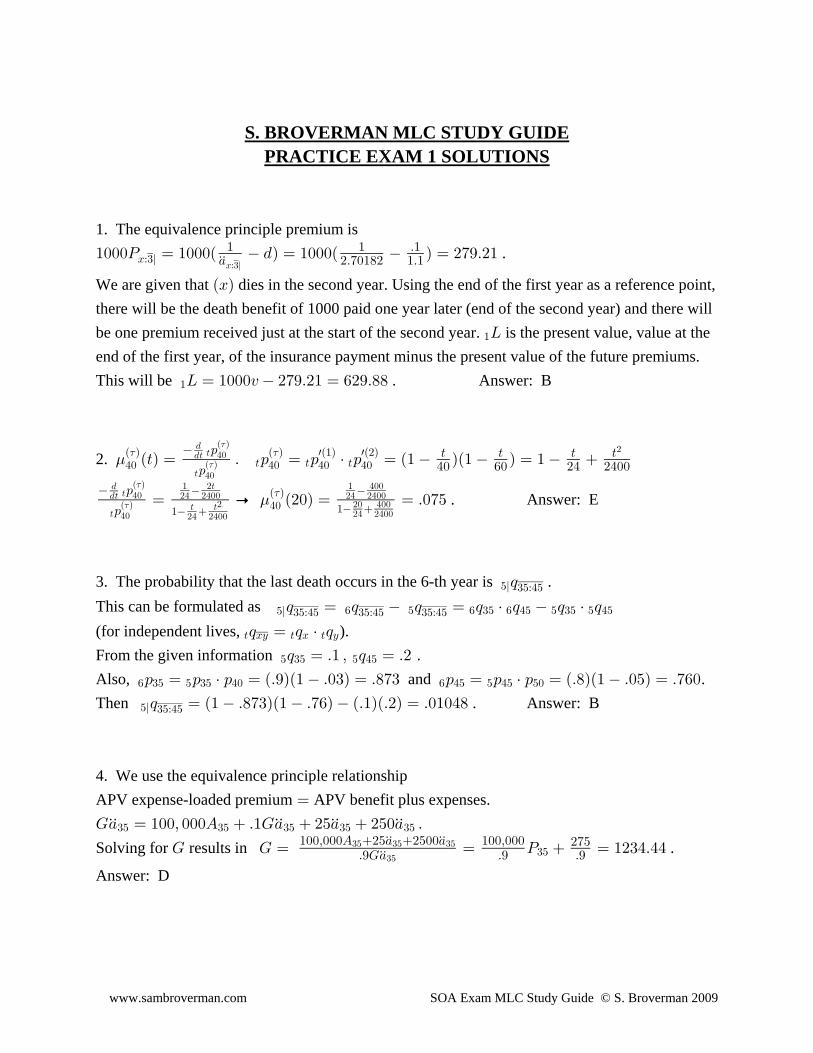
1. The equivalence principle premium is"!!!T œ "!!!Ð .Ñ œ "!!!Ð Ñ œ #(*Þ#"BÀ$l
" " Þ"+ #Þ(!")# "Þ"ÞÞBÀ$l
.
We are given that dies in the second year. Using the end of the first year as a reference point,ÐBÑ
there will be the death benefit of 1000 paid one year later (end of the second year) and there willbe one premium received just at the start of the second year. is the present value, value at the"P
end of the first year, of the insurance payment minus the present value of the future premiums.This will be . Answer: B"P œ "!!!@ #(*Þ#" œ '#*Þ))
2. .%! %! %! %!Ð Ñ Ð Ñ wÐ"Ñ wÐ#Ñ
> > >7 7Ð>Ñ œ Þ : œ : † : œ Ð" ÑÐ" Ñ œ "
:
:
> > > >%! '! #% #%!!
..> > %!
Ð Ñ
> %!Ð Ñ
#7
7
:
:
..> > %!
Ð Ñ
> %!Ð Ñ
" #> " %!!#% #%!! #% #%!!
> >#% #%!!
# #! %!!#% #%!!
7
7 œ p Ð#!Ñ œ œ Þ!(&
" %!Ð Ñ
" . Answer: E.
7
3. The probability that the last death occurs in the 6-th year is .&l $&À%&;
This can be formulated as &l $&À%& $&À%& $&À%&' & ' $& ' %& & $& & %&; œ ; ; œ ; † ; ; † ;
(for independent lives, ).> BC > B > C; œ ; † ;
From the given information .& $& & %&; œ Þ" ß ; œ Þ#
Also, and .' $& & $& %! ' %& & %& &!: œ : † : œ ÐÞ*ÑÐ" Þ!$Ñ œ Þ)($ : œ : † : œ ÐÞ)ÑÐ" Þ!&Ñ œ Þ('!
Then . Answer: B&l $&À%&; œ Ð" Þ)($ÑÐ" Þ('Ñ ÐÞ"ÑÐÞ#Ñ œ Þ!"!%)
4. We use the equivalence principle relationshipAPV expense-loaded premium APV benefit plus expenses.œ
K+ œ "!!ß !!!E Þ"K+ #&+ #&!+ ÞÞÞ ÞÞ ÞÞ ÞÞ$& $& $& $& $&
Solving for results in .K K œ œ T œ "#$%Þ%%"!!ß!!!E #&+ #&!!+ "!!ß!!!
ÞÞ ÞÞ
Þ*K+ Þ* Þ*ÞÞ
#(&$& $& $&
$&$&
Answer: D
www.sambroverman.com SOA Exam MLC Study Guide © S. Broverman 2009
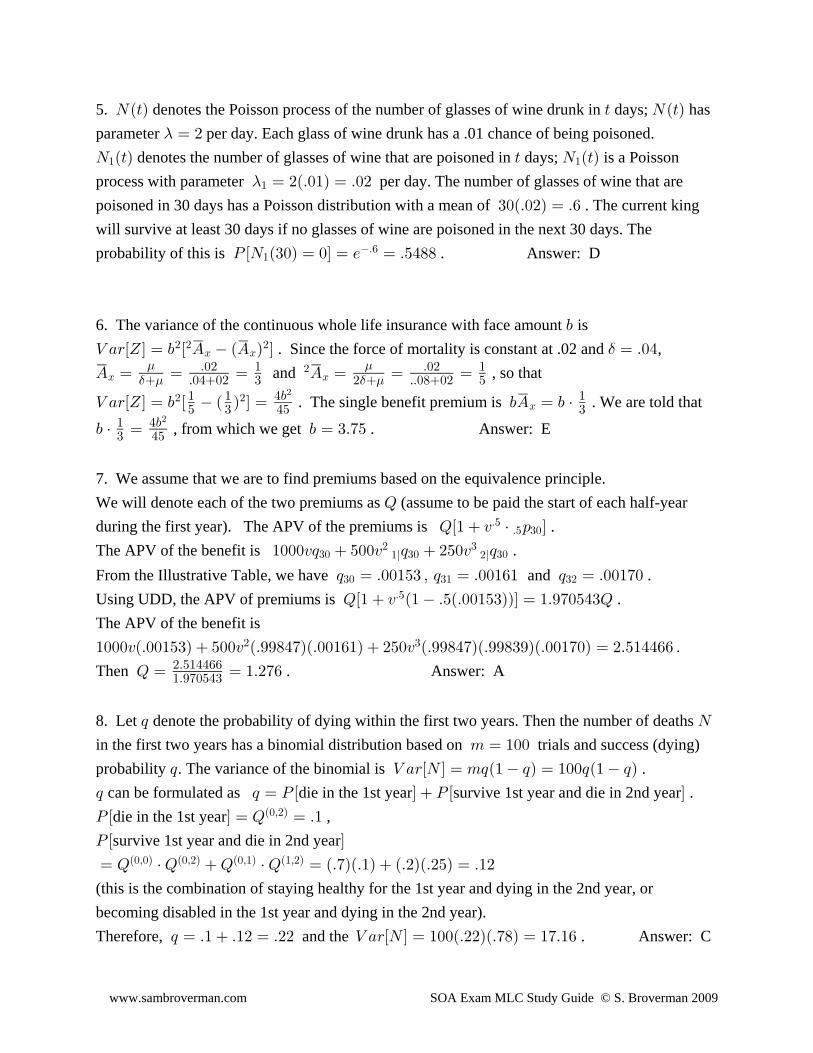
5. denotes the Poisson process of the number of glasses of wine drunk in days; hasRÐ>Ñ > RÐ>Ñ
parameter per day. Each glass of wine drunk has a .01 chance of being poisoned.- œ #
R Ð>Ñ > R Ð>Ñ" " denotes the number of glasses of wine that are poisoned in days; is a Poissonprocess with parameter per day. The number of glasses of wine that are-" œ #ÐÞ!"Ñ œ Þ!#
poisoned in 30 days has a Poisson distribution with a mean of . The current king$!ÐÞ!#Ñ œ Þ'
will survive at least 30 days if no glasses of wine are poisoned in the next 30 days. Theprobability of this is . Answer: DT ÒR Ð$!Ñ œ !Ó œ / œ Þ&%))"
Þ'
6. The variance of the continuous whole life insurance with face amount is,
Z +<Ò^Ó œ , Ò E ÐE Ñ Ó œ Þ!% # # #
B B . Since the force of mortality is constant at .02 and ,$
E œ œ œ E œ œ œ
B B#. .
$ . $ . !%!# $ # Þ!)!# &Þ!# " Þ!# "
. . and , so that
Z +<Ò^Ó œ , Ò Ð Ñ Ó œ ,E œ , †# #
B" " %, "& $ %& $
#
. The single benefit premium is . We are told that
, † œ , œ $Þ(&" %,$ %&
#
, from which we get . Answer: E
7. We assume that we are to find premiums based on the equivalence principle.We will denote each of the two premiums as (assume to be paid the start of each half-yearU
during the first year). The APV of the premiums is .UÒ" @ † : ÓÞ&Þ& $!
The APV of the benefit is ."!!!@; &!!@ ; #&!@ ;$! $! $!# $"l #l
From the Illustrative Table, we have and .; œ Þ!!"&$ ß ; œ Þ!!"'" ; œ Þ!!"(!$! $" $#
Using UDD, the APV of premiums is .UÒ" @ Ð" Þ&ÐÞ!!"&$ÑÑÓ œ "Þ*(!&%$UÞ&
The APV of the benefit is"!!!@ÐÞ!!"&$Ñ &!!@ ÐÞ**)%(ÑÐÞ!!"'"Ñ #&!@ ÐÞ**)%(ÑÐÞ**)$*ÑÐÞ!!"(!Ñ œ #Þ&"%%'' Þ# $
Then . Answer: AU œ œ "Þ#('#Þ&"%%''"Þ*(!&%$
8. Let denote the probability of dying within the first two years. Then the number of deaths ; R
in the first two years has a binomial distribution based on trials and success (dying)7 œ "!!
probability . The variance of the binomial is .; Z +<ÒRÓ œ 7;Ð" ;Ñ œ "!!;Ð" ;Ñ
; ; œ T Ò Ó T Ò Ó can be formulated as die in the 1st year survive 1st year and die in 2nd year .T Ò Ó œ U œ Þ"die in the 1st year ,Ð!ß#Ñ
T Ò Ósurvive 1st year and die in 2nd yearœ U † U U † U œ ÐÞ(ÑÐÞ"Ñ ÐÞ#ÑÐÞ#&Ñ œ Þ"#Ð!ß!Ñ Ð!ß#Ñ Ð!ß"Ñ Ð"ß#Ñ
(this is the combination of staying healthy for the 1st year and dying in the 2nd year, orbecoming disabled in the 1st year and dying in the 2nd year).Therefore, and the . Answer: C; œ Þ" Þ"# œ Þ## Z +<ÒRÓ œ "!!ÐÞ##ÑÐÞ()Ñ œ "(Þ"'
www.sambroverman.com SOA Exam MLC Study Guide © S. Broverman 2009
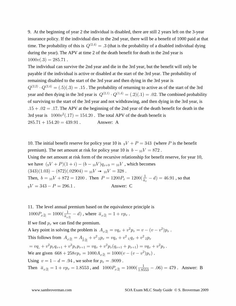
9. At the beginning of year 2 the individual is disabled, there are still 2 years left on the 3-yearinsurance policy. If the individual dies in the 2nd year, there will be a benefit of 1000 paid at thattime. The probability of this is (that is the probability of a disabled individual dyingU œ Þ$Ð#ß%Ñ
during the year). The APV at time 2 of the death benefit for death in the 2nd year is"!!!@ÐÞ$Ñ œ #)&Þ(" .The individual can survive the 2nd year and die in the 3rd year, but the benefit will only bepayable if the individual is active or disabled at the start of the 3rd year. The probability ofremaining disabled to the start of the 3rd year and then dying in the 3rd year isU † U œ ÐÞ&ÑÐÞ$Ñ œ Þ"&Ð#ß#Ñ Ð#ß%Ñ . The probability of returning to active as of the start of the 3rdyear and then dying in the 3rd year is The combined probabilityU † U œ ÐÞ#ÑÐÞ"Ñ œ Þ!#ÞÐ#ß"Ñ Ð"ß%Ñ
of surviving to the start of the 3rd year and not withdrawing, and then dying in the 3rd year, isÞ"& Þ!# œ Þ"(. The APV at the beginning of the 2nd year of the death benefit for death in the3rd year is . The total APV of the death benefit is"!!!@ ÐÞ"(Ñ œ "&%Þ#!#
#)&Þ(" "&%Þ#! œ %$*Þ*" . Answer: A
10. The initial benefit reserve for policy year 10 is (where is the benefit*Z T œ $%$ T
premium). The net amount at risk for policy year 10 is ., Z œ )(#"!
Using the net amount at risk form of the recursive relationship for benefit reserve, for year 10,we have , which becomesÐ Z TÑÐ" 3Ñ Ð, Z Ñ; œ Z* "! B* "!
Ð$%$ÑÐ"Þ!$Ñ Ð)(#ÑÐÞ!#*!%Ñ œ Z p Z œ $#)"! "! .Then, . Then , so that, œ Z )(# œ "#!! T œ "#!!T œ "#!!Ð .Ñ œ %'Þ*""! B
"+ÞÞB
*Z œ $%$ T œ #*'Þ" . Answer: C
11. The level annual premium based on the equivalence principle is"!!!T œ "!!!Ð .Ñ + œ " @:
ÞÞBÀ#l BÀ#l B
"+ÞÞBÀ#l
, where .
If we find we can find the premium.:B
A key point in solving the problem is .E œ @; @ : œ @ Ð@ @ Ñ:BÀ#l B B B# #
This follows from E œ E @ : œ @; @ ; @ :BÀ#l BÀ#l"
# # ## B B B # B"l
œ @; @ : ; @ : : œ @; @ : Ð; : Ñ œ @; @ : ÞB
# # # #B B" B B" B B B" B" B B
We are given .'') #&)@: œ "!!!E œ "!!!Ð@ Ð@ @ Ñ: ÑB BBÀ#l#
Using , we solve for .@ œ " . œ Þ*% : œ Þ*!**B
Then , and . Answer: B+ œ " @: œ "Þ)&&$ "!!!T œ "!!!Ð Þ!'Ñ œ %(*ÞÞBÀ#l BÀ#lB
""Þ)&&$
www.sambroverman.com SOA Exam MLC Study Guide © S. Broverman 2009
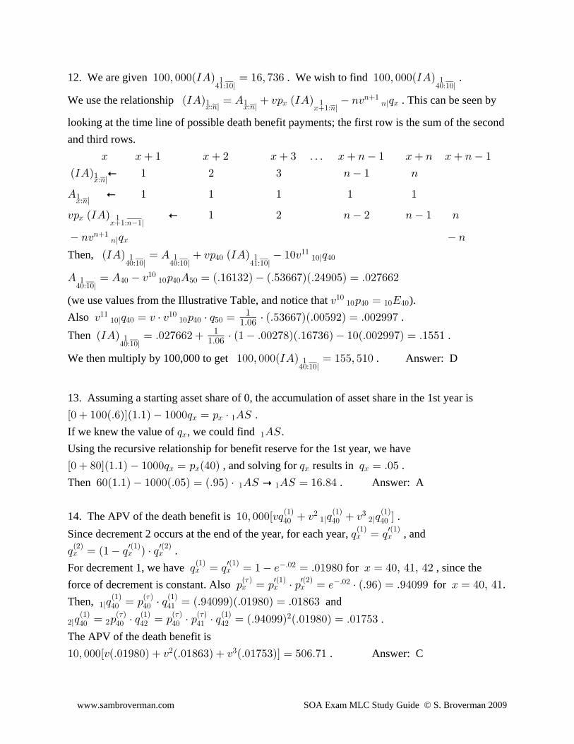
12. We are given . We wish to find ."!!ß !!!ÐMEÑ œ "'ß ($' "!!ß !!!ÐMEÑ%"À"!l %!À"!l" "
We use the relationship . This can be seen byÐMEÑ œ E @: ÐMEÑ 8@ ;BÀ8l BÀ8l" " "B B
B"À8l
8"8l
looking at the time line of possible death benefit payments; the first row is the sum of the secondand third rows. B B " B # B $ Þ Þ Þ B 8 " B 8 B 8 "
ÐMEÑ o " # $ 8 " 8BÀ8l"
E o " " " " "BÀ8l"
@: ÐMEÑ o " # 8 # 8 " 8BB"À8"l"
8@ ; 88"8l B
Then, ÐMEÑ œ E @: ÐMEÑ "!@ ;%!À"!l %!À"!l %"À"!l" " "%! %!
"""!l
E œ E @ : E œ ÐÞ"'"$#Ñ ÐÞ&$''(ÑÐÞ#%*!&Ñ œ Þ!#(''#%!À"!l" %! "! %! &!
"!
(we use values from the Illustrative Table, and notice that ).@ : œ I"!"! %! "! %!
Also .@ ; œ @ † @ : † ; œ † ÐÞ&$''(ÑÐÞ!!&*#Ñ œ Þ!!#**("" "!"!l %! "! %! &!
""Þ!'
Then .ÐMEÑ œ Þ!#(''# † Ð" Þ!!#()ÑÐÞ"'($'Ñ "!ÐÞ!!#**(Ñ œ Þ"&&"%!À"!l"
""Þ!'
We then multiply by 100,000 to get . Answer: D"!!ß !!!ÐMEÑ œ "&&ß &"!%!À"!l"
13. Assuming a starting asset share of 0, the accumulation of asset share in the 1st year isÒ! "!!ÐÞ'ÑÓÐ"Þ"Ñ "!!!; œ : † EWB B " .If we knew the value of , we could find .; EWB "
Using the recursive relationship for benefit reserve for the 1st year, we haveÒ! )!ÓÐ"Þ"Ñ "!!!; œ : Ð%!Ñ ; ; œ Þ!&B B B B , and solving for results in .Then . Answer: A'!Ð"Þ"Ñ "!!!ÐÞ!&Ñ œ ÐÞ*&Ñ † EW p EW œ "'Þ)%" "
14. The APV of the death benefit is ."!ß !!!Ò@; @ ; @ ; Ó%! %! %!Ð"Ñ Ð"Ñ Ð"Ñ# $
"l #l
Since decrement 2 occurs at the end of the year, for each year, , and; œ ;B BÐ"Ñ wÐ"Ñ
; œ Ð" ; Ñ † ;B B BÐ#Ñ wÐ"Ñ wÐ#Ñ .
For decrement 1, we have for , since the; œ ; œ " / œ Þ!"*)! B œ %!ß %"ß %#B BÐ"Ñ wÐ"Ñ Þ!#
force of decrement is constant. Also for .: œ : † : œ / † ÐÞ*'Ñ œ Þ*%!** B œ %!ß %"B B BÐ Ñ wÐ"Ñ wÐ#Ñ Þ!#7
Then, and"l %! %! %"Ð"Ñ Ð Ñ Ð"Ñ
; œ : † ; œ ÐÞ*%!**ÑÐÞ!"*)!Ñ œ Þ!")'$7
#l %! %! %# %! %" %#Ð"Ñ Ð Ñ Ð"Ñ Ð Ñ Ð Ñ Ð"Ñ
##; œ : † ; œ : † : † ; œ ÐÞ*%!**Ñ ÐÞ!"*)!Ñ œ Þ!"(&$
7 7 7 .The APV of the death benefit is"!ß !!!Ò@ÐÞ!"*)!Ñ @ ÐÞ!")'$Ñ @ ÐÞ!"(&$ÑÓ œ &!'Þ("# $ . Answer: C
www.sambroverman.com SOA Exam MLC Study Guide © S. Broverman 2009
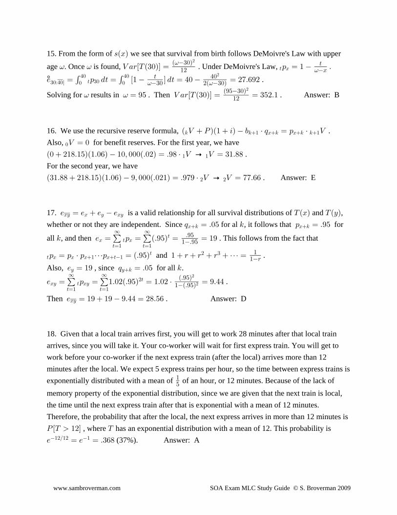
15. From the form of we see that survival from birth follows DeMoivre's Law with upper=ÐBÑ
age . Once is found, . Under DeMoivre's Law, = = Z +<ÒX Ð$!ÑÓ œ : œ " ÞÐ $!Ñ
"# B>=
=
#
> B
/ œ : .> œ Ò" Ó .> œ %! œ #(Þ'*#° .$!À%!l ! !%! %!
> $!' ' > %!$! #Ð $!Ñ= =
#
Solving for results in . Then . Answer: B= = œ *& Z +<ÒX Ð$!ÑÓ œ œ $&#Þ"Ð*&$!Ñ
"#
#
16. We use the recursive reserve formula, .Ð Z TÑÐ" 3Ñ , † ; œ : † Z5 5" B5 B5 5"
Also, for benefit reserves. For the first year, we have!Z œ !
Ð! #")Þ"&ÑÐ"Þ!'Ñ "!ß !!!ÐÞ!#Ñ œ Þ*) † Z p Z œ $"Þ))" " .For the second year, we haveÐ$"Þ)) #")Þ"&ÑÐ"Þ!'Ñ *ß !!!ÐÞ!#"Ñ œ Þ*(* † Z p Z œ ((Þ''# # . Answer: E
17. is a valid relationship for all survival distributions of and ,/ œ / / / XÐBÑ X ÐCÑBC B C BC
whether or not they are independent. Since for al , it follows that for; œ Þ!& 5 : œ Þ*&B5 B5
all , and then . This follows from the fact that5 / œ : œ ÐÞ*&Ñ œ œ "*B > B>œ" >œ"
∞ ∞> Þ*&
"Þ*&
> B B B" B>"> # $: œ : † : â: œ ÐÞ*&Ñ " < < < â œ and ."
"<
Also, , since for all ./ œ "* ; œ Þ!& 5C C5
/ œ : œ "Þ!#ÐÞ*&Ñ œ "Þ!# † œ *Þ%%BC > BC>œ" >œ"
∞ ∞#> ÐÞ*&Ñ
"ÐÞ*&Ñ
#
# .
Then . Answer: D/ œ "* "* *Þ%% œ #)Þ&'BC
18. Given that a local train arrives first, you will get to work 28 minutes after that local trainarrives, since you will take it. Your co-worker will wait for first express train. You will get towork before your co-worker if the next express train (after the local) arrives more than 12minutes after the local. We expect 5 express trains per hour, so the time between express trains isexponentially distributed with a mean of of an hour, or 12 minutes. Because of the lack of"
&
memory property of the exponential distribution, since we are given that the next train is local,the time until the next express train after that is exponential with a mean of 12 minutes.Therefore, the probability that after the local, the next express arrives in more than 12 minutes isT ÒX "#Ó X , where has an exponential distribution with a mean of 12. This probability is/ œ / œ Þ$')"#Î"# " (37%). Answer: A
www.sambroverman.com SOA Exam MLC Study Guide © S. Broverman 2009
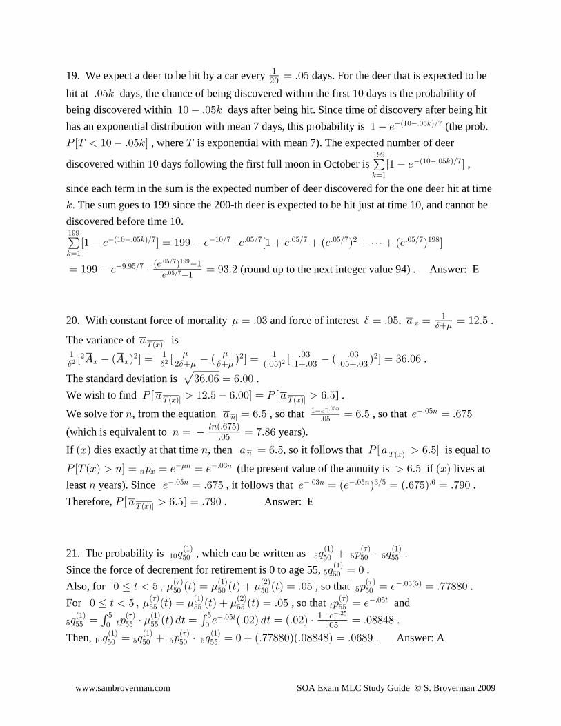
19. We expect a deer to be hit by a car every days. For the deer that is expected to be"#! œ Þ!&
hit at days, the chance of being discovered within the first 10 days is the probability ofÞ!&5
being discovered within days after being hit. Since time of discovery after being hit"! Þ!&5
has an exponential distribution with mean 7 days, this probability is (the prob." /Ð"!Þ!&5ÑÎ(
T ÒX "! Þ!&5Ó X , where is exponential with mean 7). The expected number of deer
discovered within 10 days following the first full moon in October is ,5œ"
"**Ð"!Þ!&5ÑÎ(Ò" / Ó
since each term in the sum is the expected number of deer discovered for the one deer hit at time5. The sum goes to 199 since the 200-th deer is expected to be hit just at time 10, and cannot bediscovered before time 10.
5œ"
"**Ð"!Þ!&5ÑÎ( "!Î( Þ!&Î( Þ!&Î( Þ!&Î( # Þ!&Î( "*)Ò" / Ó œ "** / † / Ò" / Ð/ Ñ â Ð/ Ñ Ó
œ "** / † œ *$Þ#*Þ*&Î( Ð/ Ñ "/ "
Þ!&Î( "**
Þ!&Î( (round up to the next integer value 94) . Answer: E
20. With constant force of mortality and force of interest , .. $œ Þ!$ œ Þ!& + œ œ "#Þ&B
"$ .
The variance of is+XÐBÑl
" " " Þ!$ Þ!$# ÐÞ!&Ñ Þ"Þ!$ Þ!&Þ!$$ $ $ . $ .. .
# # #Ò E ÐE Ñ Ó œ Ò Ð Ñ Ó œ Ò Ð Ñ Ó œ $'Þ!' # # # #
B B .
The standard deviation is .È$'Þ!' œ 'Þ!!
We wish to find ] .T Ò + "#Þ& 'Þ!!Ó œ T Ò + 'Þ& XÐBÑl X ÐBÑl
We solve for , from the equation , so that , so that 8 + œ 'Þ& œ 'Þ& / œ Þ'(&8l
"/Þ!&
Þ!&8Þ!&8
(which is equivalent to years).8 œ œ (Þ)'68ÐÞ'(&Ñ
Þ!&
If dies exactly at that time , then , so it follows that is equal toÐBÑ 8 + œ 'Þ& T Ò + 'Þ&Ó 8l XÐBÑl
T ÒX ÐBÑ 8Ó œ : œ / œ / 'Þ& ÐBÑ8 B 8 Þ!$8. (the present value of the annuity is if lives at
least years). Since , it follows that .8 / œ Þ'(& / œ Ð/ Ñ œ ÐÞ'(&Ñ œ Þ(*!Þ!&8 Þ!$8 Þ!&8 $Î& Þ'
Therefore, ] . Answer: ET Ò + 'Þ& œ Þ(*!XÐBÑl
21. The probability is , which can be written as ."! & & &&! &! &! &&Ð"Ñ Ð"Ñ Ð Ñ Ð"Ñ
; ; : † ;7
Since the force of decrement for retirement is 0 to age 55, .& &!Ð"Ñ
; œ !
Also, for , so that .! Ÿ > & ß Ð>Ñ œ Ð>Ñ Ð>Ñ œ Þ!& : œ / œ Þ(())!. . .&! &! &! &!Ð Ñ Ð"Ñ Ð#Ñ Ð Ñ
&Þ!&Ð&Ñ7 7
For , so that and! Ÿ > & ß Ð>Ñ œ Ð>Ñ Ð>Ñ œ Þ!& : œ /. . .&& && && &&Ð Ñ Ð"Ñ Ð#Ñ Ð Ñ
>Þ!&>7 7
& >&& && &&Ð"Ñ Ð Ñ Ð"Ñ
! !& & Þ!&>; œ : † Ð>Ñ .> œ / ÐÞ!#Ñ .> œ ÐÞ!#Ñ † œ Þ!))%)' '7
. "/Þ!&
Þ#&
.Then, . Answer: A"! & & &&! &! &! &&
Ð"Ñ Ð"Ñ Ð Ñ Ð"Ñ; œ ; : † ; œ ! ÐÞ(())!ÑÐÞ!))%)Ñ œ Þ!')*
7
www.sambroverman.com SOA Exam MLC Study Guide © S. Broverman 2009
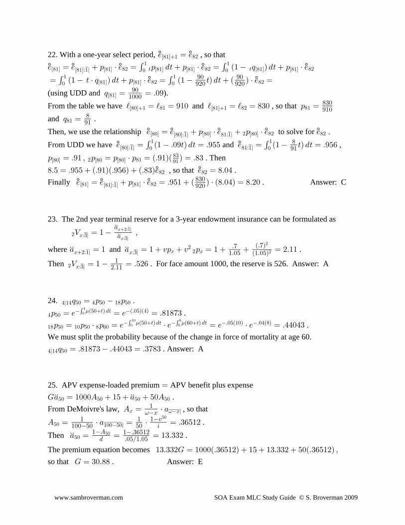
22. With a one-year select period, , so that° °/ œ /Ò)"Ó" )#
/ œ / : † / œ : .> : † / œ Ð" ; Ñ .> : † /° ° ° ° °Ò)"Ó Ò)"Ó Ò)"Ó Ò)"Ó Ò)"Ó Ò)"ÓÒ)"ÓÀ"l )# > )# > )#! !" "' '
œ Ð" > † ; Ñ .> : † / œ Ð" >Ñ .> Ð Ñ † / œ' '! !" "
Ò)"Ó Ò)"Ó )# )#° °*! *!*#! *#!
(using UDD and ).; œ œ Þ!*Ò)"Ó*!
"!!!
From the table we have and , so that j œ j œ *"! j œ j œ )$! : œÒ)!Ó" Ò)"Ó")" )# )")$!*"!
and .; œ)")*"
Then, we use the relationship to solve for .° ° ° ° °/ œ / : † / : † / /Ò)!Ó Ò)!Ó Ò)!ÓÒ)!ÓÀ"l )"À"l # )# )#
From UDD we have and ,° °/ œ Ð" Þ!*>Ñ .> œ Þ*&& / œ Ð" >Ñ .> œ Þ*&'Ò)!ÓÀ"l )"À"l! !" "' ' )
*"
: œ Þ*" ß : œ : † : œ ÐÞ*"ÑÐ Ñ œ Þ)$Ò)!Ó Ò)! Ò)!Ó# )")$*" . Then
)Þ& œ Þ*&& ÐÞ*"ÑÐÞ*&'Ñ ÐÞ)$Ñ/ / œ )Þ!%° ° , so that .)# )#
Finally . Answer: C° ° °/ œ / : † / œ Þ*&" Ð Ñ † Ð)Þ!%Ñ œ )Þ#!Ò)"Ó Ò)"ÓÒ)"ÓÀ"l )#)$!*#!
23. The 2nd year terminal reserve for a 3-year endowment insurance can be formulated as
# BÀ$lZ œ " ß+ÞÞ
+ÞÞB#À"l
BÀ$l
where and .+ œ " + œ " @: @ : œ " œ #Þ""ÞÞ ÞÞB#À"l BÀ l B # B
#3
Þ("Þ!& Ð"Þ!&Ñ
ÐÞ(Ñ#
#
Then . For face amount 1000, the reserve is 526. Answer: A# BÀ$lZ œ " œ Þ&#'"#Þ""
24. .%l"% &! % &! ") &!; œ : :
% &! Ð&!>Ñ .> ÐÞ!&ÑÐ%Ñ: œ / œ / œ Þ)")($'
!%. .
") &! "! &! ) '! Ð&!>Ñ .> Ð'!>Ñ .> Þ!&Ð"!Ñ Þ!%Ð)Ñ: œ : † : œ / † / œ / † / œ Þ%%!%$' '
! !"! ). . .
We must split the probability because of the change in force of mortality at age 60.
%l"% &!; œ Þ)")($ Þ%%!%$ œ Þ$()$ . Answer: A
25. APV expense-loaded premium APV benefit plus expenseœ
K+ œ "!!!E "& + &!EÞÞ ÞÞ&! &! &! &! .
From DeMoivre's law, , so thatE œ † +B Bl"B= =
E œ † + œ † œ Þ$'&"#&! "!!&!l" " "@
"!!&! &! 3
&!
.
Then .+ œ œ œ "$Þ$$#ÞÞ&!
"E. Þ!&Î"Þ!&
"Þ$'&"#&!
The premium equation becomes "$Þ$$#K œ "!!!ÐÞ$'&"#Ñ "& "$Þ$$# &!ÐÞ$'&"#Ñ ß
so that . Answer: EK œ $!Þ))
www.sambroverman.com SOA Exam MLC Study Guide © S. Broverman 2009
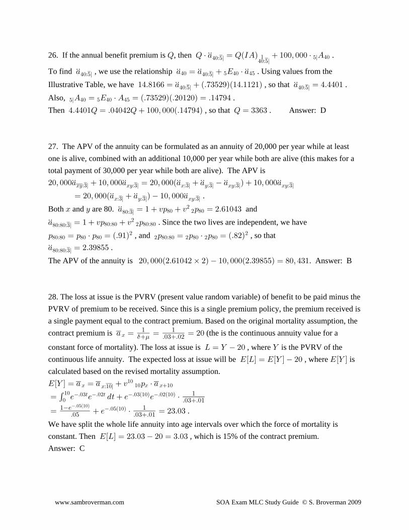
26. If the annual benefit premium is , then .U U † + œ UÐMEÑ "!!ß !!! † EÞÞ%!À&l
%!À&l" &l %!
To find , we use the relationship . Using values from the+ + œ + I † +ÞÞ ÞÞ ÞÞ ÞÞ%!À&l %!À&l%! & %! %&
Illustrative Table, we have , so that ."%Þ)"'' œ + ÐÞ($&#*ÑÐ"%Þ""#"Ñ + œ %Þ%%!"ÞÞ ÞÞ%!À&l %!À&l
Also, .&l %! & %! %&E œ I † E œ ÐÞ($&#*ÑÐÞ#!"#!Ñ œ Þ"%(*%
Then , so that . Answer: D%Þ%%!"U œ Þ!%!%#U "!!ß !!!ÐÞ"%(*%Ñ U œ $$'$
27. The APV of the annuity can be formulated as an annuity of 20,000 per year while at leastone is alive, combined with an additional 10,000 per year while both are alive (this makes for atotal payment of 30,000 per year while both are alive). The APV is#!ß !!!+ "!ß !!!+ œ #!ß !!!Ð+ + + Ñ "!ß !!!+
ÞÞ ÞÞ ÞÞ ÞÞ ÞÞ ÞÞBCÀ$l BCÀ$l BÀ$l CÀ$l BCÀ$l BCÀ$l
.œ #!ß !!!Ð+ + Ñ "!ß !!!+ÞÞ ÞÞ ÞÞBÀ$l CÀ$l BCÀ$l
Both and are 80. andB C + œ " @: @ : œ #Þ'"!%$ÞÞ)!À$l )! # )!
#
+ œ " @: @ :ÞÞ)!À)!À$l )!À)! # )!À)!
# . Since the two lives are independent, we have
: œ : † : œ ÐÞ*"Ñ : œ : † : œ ÐÞ)#Ñ)!À)! )! )! # )!À)! # )! # )!# # , and , so that
+ œ #Þ$*)&&ÞÞ)!À)!À$l .
The APV of the annuity is . Answer: B#!ß !!!Ð#Þ'"!%# ‚ #Ñ "!ß !!!Ð#Þ$*)&&Ñ œ )!ß %$"
28. The loss at issue is the PVRV (present value random variable) of benefit to be paid minus thePVRV of premium to be received. Since this is a single premium policy, the premium received isa single payment equal to the contract premium. Based on the original mortality assumption, thecontract premium is (the is the continuous annuity value for a+ œ œ œ #!
B" " Þ!$Þ!#$ .
constant force of mortality). The loss at issue is , where is the PVRV of theP œ ] #! ]
continuous life annuity. The expected loss at issue will be , where isIÒPÓ œ IÒ] Ó #! IÒ] Ó
calculated based on the revised mortality assumption.IÒ] Ó œ + œ + @ : † +
B "! B B"!BÀ"!l"!
œ / / .> / / †'!"! Þ!$> Þ!#> Þ!$Ð"!Ñ Þ!#Ð"!Ñ "
Þ!$Þ!"
œ / † œ #$Þ!$"/ "Þ!& Þ!$Þ!"
Þ!&Ð"!ÑÞ!&Ð"!Ñ .
We have split the whole life annuity into age intervals over which the force of mortality isconstant. Then , which is 15% of the contract premium. IÒPÓ œ #$Þ!$ #! œ $Þ!$
Answer: C
www.sambroverman.com SOA Exam MLC Study Guide © S. Broverman 2009
29. The single benefit premium per person is ."!!!@; &!!@ ;$! $!#"l
Using the Illustrative Table, we have and .; œ Þ!!"&$ ; œ : † ; œ Þ!!"'!(&$! $! $! $""l
The single benefit premium is . Since this is a single benefit premium, the expected size#Þ"&)($
of the fund at the end of the 2-year term is 0. The actual fund progresses in the following way."!!!Ð#Þ"&)($Ñ œ #"&)Þ($ is collected at the start of the first year.At the end of the first year, with interest minus death benefit, the fund value is#"&)Þ($Ð"Þ!(Ñ "!!! œ "$!*Þ)% .With interest minus death benefits to the end of the second year, the fund value is"$!*Þ)%Ð"Þ!'*Ñ &!! œ *!!Þ# . Answer: C
30. is the probability that for and , alive at age 64 and 85, will survive theU ÐBÑ ÐCÑ ÐBÑ"!Ð"ß#Ñ
year, but will die within the year. This probability that (64) survives the year is for ,ÐCÑ : ÐBÑ'%
which is . The probability that (85) dies during the year is for , which = Ð'&Ñ= Ð'%ÑB
Bœ Þ*)'!"$ ; ÐCÑ)&
is" œ Þ!'''( ÐCÑ œ "!! Þ
= Ð)'Ñ= Ð)&ÑC
C ( 's mortality follows DeMoivre's Law with )=
Then, . Answer: EU œ : † ; œ ÐÞ*)'!"$ÑÐÞ!'''(Ñ œ Þ!''"! '% )&Ð"ß#Ñ B C