137

139

Scale effects in biodiversity and biological control Scale effects in biodiversity and biological control

138

1 Definitions of scale, and an outline for this chapter

The structure of agricultural landscapes is likely to influence organisms living in these landscapes, and in particular, insect pests and their natural enemies (Gámez-Virués et al., this volume). Interactions at a local scale (for example an individual field) are likely to be influenced by processes acting at larger scales (for example the surroundings of that field; Plate 9.1). This is often called scale dependence or context dependence (Pearson 2002).

This chapter serves as an introduction to the de-sign and analysis of studies on biocontrol at differ-ent spatial scales. Spatial scale can be described by two factors, grain and extent (Wiens 1989; Fortin and Dale 2005). Grain is the size of an individual sampling unit (for example a plot measuring 4 m²); extent is the total size of the study area (for example a landscape measuring 100 ha). The grain size used for individual study units should be carefully cho-sen to match the spatial structure of the phenom-enon being studied. For example, a grain size of 0.5 cm could be necessary in a study of insects inhabit-ing wheat stems (where the spatial arrangement of damaged vs. intact wheat stems is of interest). In addition, the grain size can also be important when it comes to data analysis - that is, when data are aggregated for statistical analysis. Hence, “spatial scale” can refer to an individual study organism, an individual sampling unit, or an individual unit of

statistical analysis (see also Dungan et al. 2002).

Knowing now what we mean by “scale”, we may now ask: How can scaling effects be included in studies on pest control? Before addressing scale ef-fects out in the landscape, it is often useful to start with smaller-scale laboratory systems where it is easier to control for confounding variables. We therefore start this chapter with an introduction to the problem of “upscaling”, that is, the extrapola-tion from smaller to larger scales. We then move on to the landscape scale, and provide an overview of field methods used to study the movement of or-ganisms through the landscape. This section is fol-lowed by two sections on data analysis and mod-elling. Finally, we conclude the chapter with some guidelines likely to be useful for practitioners who want to incorporate scale effects in their own bio-control studies.

2 From the laboratory to the field: upscaling problems

In traditional biocontrol studies, it is often neces-sary to start with a series of smaller-scale laboratory experiments before moving to the field scale. For example, we need to understand the host specific-ity of biocontrol agents, or the food plant spectrum of individual insect herbivores, before we can begin to understand what is happening in the field. Often, the underlying interactions between the biological

Plate 9.1: Scale transitions and landscape complexity in agroecosystems. (a) Wheat spikes are attacked by pest insects (e.g. aphids) in-teracting with biocontrol agents on a local scale; (b) a complex agricultural landscape near Holzminden (Central Germany); (c) a simple agricultural landscape in the cereal plain of Chizé (France). All photographs by C. Scherber.

Published as:

Scherber C, Lavandero B, Meyer KM, Perovic D, Visser U, Wiegand K, Tscharntke T (2012) Scale effects in biodiversity and biological control: methods and statistical analysis. Book chapter in: Gurr GM, Wratten SD, Snyder WE (eds.) Biodiversity and Insect Pests: key issues for sustainable manage-ment. Wiley Blackwell.

141

Scale effects in biodiversity and biological control Scale effects in biodiversity and biological control

140

Microbial systems can be a worthwhile starting point to test the performance of current and new upscaling approaches before transferring the re-sults to insect biological control agents.

The lack of overarching upscaling approaches in-dicates that, probably, each scale requires its own approach, so that we should advance the coupling of existing approaches rather than aiming at devel-oping the universal up-scaling approach (Meyer et al., 2010). One example of a coupled approach is the pattern-oriented modelling strategy (Grimm et al., 2005) where small-scale mechanisms are derived from large-scale patterns. Pattern-oriented model-ling can be used to distinguish between alternative hypotheses on the transition from one scale to the other and thus identify the most appropriate up-scaling approach for a particular biological control study.

Overall, upscaling studies show that it can be dif-ficult to compare results obtained in laboratory systems to the field or landscape scale. It is there-fore inevitable to move one step further and try to follow organisms out in the agricultural landscape. In the next section, we will see how we can track the movement of insects through real landscapes - a prerequisite for many approaches that follow.

3 Field methods for understanding landscape-scale patterns

Moving from smaller laboratory systems to the field and landscape scale, researchers often have to become detectives – simply because there is so much space available for study-organisms to hide and escape. This is not so much of a problem un-der small-scale laboratory conditions, but is central to the success or failure of large-scale field studies. Up-scaling from the laboratory to the field thus requires a whole new set of approaches to track arthropods at the large scale. During the last few decades, a series of different marking and tracking techniques have been developed to study arthro-pod movement and dispersal. These techniques can be used to identify the land uses that (1) act as sources of movement into crops, for both pests and natural enemies, and (2) act as alternative resources and resource subsidies for natural enemies. In the following brief overview of marking and tracking techniques we outline how different techniques have been used to investigate the movement and spatial ecology of arthropods and suggest areas for future focus. Due to the limits on space, however, the following section is by no means an in-depth review of this subject (more detailed reviews are highlighted in Table 9.1)

Following animals from one point to another is the basic requirement of any marking and tracking technique. The fact that “old fashioned” techniques

Purpose Method Selected references Applications

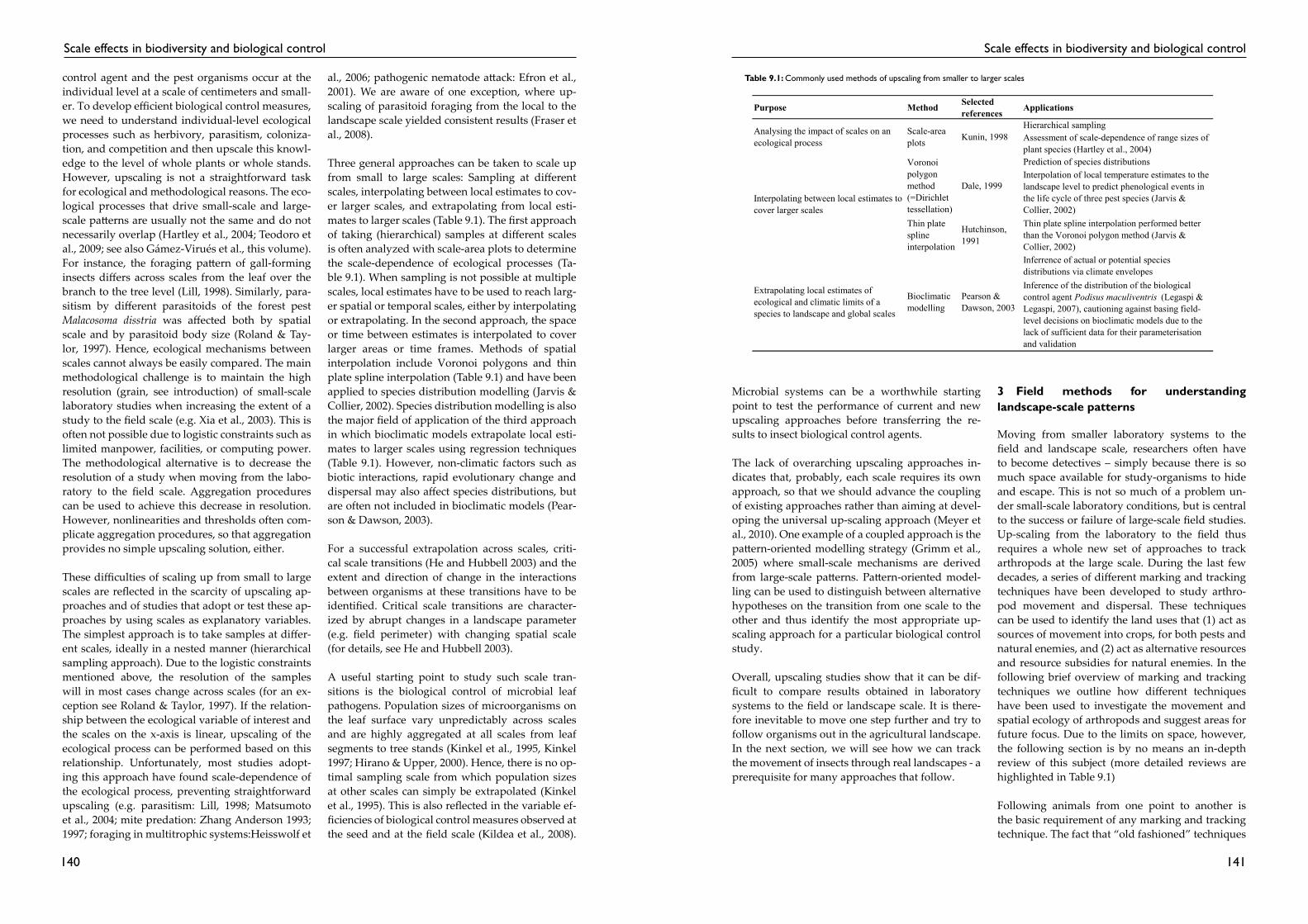
Hierarchical samplingAssessment of scale-dependence of range sizes of plant species (Hartley et al., 2004)Prediction of species distributionsInterpolation of local temperature estimates to the landscape level to predict phenological events in the life cycle of three pest species (Jarvis & Collier, 2002)

Thin plate spline interpolation

Hutchinson, 1991

Thin plate spline interpolation performed better than the Voronoi polygon method (Jarvis & Collier, 2002)Inferrence of actual or potential species distributions via climate envelopesInference of the distribution of the biological control agent Podisus maculiventris (Legaspi & Legaspi, 2007), cautioning against basing field-level decisions on bioclimatic models due to the lack of sufficient data for their parameterisation and validation

Extrapolating local estimates of ecological and climatic limits of a species to landscape and global scales

Bioclimatic modelling

Pearson & Dawson, 2003

Analysing the impact of scales on an ecological process

Scale-area plots Kunin, 1998

Interpolating between local estimates to cover larger scales

Voronoi polygon method (=Dirichlet tessellation)

Dale, 1999

Table 9.1: Commonly used methods of upscaling from smaller to larger scalescontrol agent and the pest organisms occur at the individual level at a scale of centimeters and small-er. To develop efficient biological control measures, we need to understand individual-level ecological processes such as herbivory, parasitism, coloniza-tion, and competition and then upscale this knowl-edge to the level of whole plants or whole stands. However, upscaling is not a straightforward task for ecological and methodological reasons. The eco-logical processes that drive small-scale and large-scale patterns are usually not the same and do not necessarily overlap (Hartley et al., 2004; Teodoro et al., 2009; see also Gámez-Virués et al., this volume). For instance, the foraging pattern of gall-forming insects differs across scales from the leaf over the branch to the tree level (Lill, 1998). Similarly, para-sitism by different parasitoids of the forest pest Malacosoma disstria was affected both by spatial scale and by parasitoid body size (Roland & Tay-lor, 1997). Hence, ecological mechanisms between scales cannot always be easily compared. The main methodological challenge is to maintain the high resolution (grain, see introduction) of small-scale laboratory studies when increasing the extent of a study to the field scale (e.g. Xia et al., 2003). This is often not possible due to logistic constraints such as limited manpower, facilities, or computing power. The methodological alternative is to decrease the resolution of a study when moving from the labo-ratory to the field scale. Aggregation procedures can be used to achieve this decrease in resolution. However, nonlinearities and thresholds often com-plicate aggregation procedures, so that aggregation provides no simple upscaling solution, either.

These difficulties of scaling up from small to large scales are reflected in the scarcity of upscaling ap-proaches and of studies that adopt or test these ap-proaches by using scales as explanatory variables. The simplest approach is to take samples at differ-ent scales, ideally in a nested manner (hierarchical sampling approach). Due to the logistic constraints mentioned above, the resolution of the samples will in most cases change across scales (for an ex-ception see Roland & Taylor, 1997). If the relation-ship between the ecological variable of interest and the scales on the x-axis is linear, upscaling of the ecological process can be performed based on this relationship. Unfortunately, most studies adopt-ing this approach have found scale-dependence of the ecological process, preventing straightforward upscaling (e.g. parasitism: Lill, 1998; Matsumoto et al., 2004; mite predation: Zhang Anderson 1993; 1997; foraging in multitrophic systems:Heisswolf et

al., 2006; pathogenic nematode attack: Efron et al., 2001). We are aware of one exception, where up-scaling of parasitoid foraging from the local to the landscape scale yielded consistent results (Fraser et al., 2008).

Three general approaches can be taken to scale up from small to large scales: Sampling at different scales, interpolating between local estimates to cov-er larger scales, and extrapolating from local esti-mates to larger scales (Table 9.1). The first approach of taking (hierarchical) samples at different scales is often analyzed with scale-area plots to determine the scale-dependence of ecological processes (Ta-ble 9.1). When sampling is not possible at multiple scales, local estimates have to be used to reach larg-er spatial or temporal scales, either by interpolating or extrapolating. In the second approach, the space or time between estimates is interpolated to cover larger areas or time frames. Methods of spatial interpolation include Voronoi polygons and thin plate spline interpolation (Table 9.1) and have been applied to species distribution modelling (Jarvis & Collier, 2002). Species distribution modelling is also the major field of application of the third approach in which bioclimatic models extrapolate local esti-mates to larger scales using regression techniques (Table 9.1). However, non-climatic factors such as biotic interactions, rapid evolutionary change and dispersal may also affect species distributions, but are often not included in bioclimatic models (Pear-son & Dawson, 2003).

For a successful extrapolation across scales, criti-cal scale transitions (He and Hubbell 2003) and the extent and direction of change in the interactions between organisms at these transitions have to be identified. Critical scale transitions are character-ized by abrupt changes in a landscape parameter (e.g. field perimeter) with changing spatial scale (for details, see He and Hubbell 2003).

A useful starting point to study such scale tran-sitions is the biological control of microbial leaf pathogens. Population sizes of microorganisms on the leaf surface vary unpredictably across scales and are highly aggregated at all scales from leaf segments to tree stands (Kinkel et al., 1995, Kinkel 1997; Hirano & Upper, 2000). Hence, there is no op-timal sampling scale from which population sizes at other scales can simply be extrapolated (Kinkel et al., 1995). This is also reflected in the variable ef-ficiencies of biological control measures observed at the seed and at the field scale (Kildea et al., 2008).

143

Scale effects in biodiversity and biological control Scale effects in biodiversity and biological control

142

tracking techniques in biological control, especially with a focus on biodiversity, is the use of multiple markers to adapt techniques to more complex field situations; for example, to simultaneously identify multiple resources (i.e. different source habitats or different resource subsidies). The recent advances in identifying common proteins with ELISA (Hagler & Jones 2010) offers great potential in this endeavour; e.g., to use milk proteins to mark one field, or one prey species, and egg proteins to mark another field or prey species.

Great potential is also offered by combining differ-ent disciplines, for example in ’landscape genetics’. In recent years, the use of landscape genetics, which is the combination of high resolution genetic mark-ers with spatial data analysis, has been particularly relevant when assessing the influence of landscape characteristics on the genetic variability and the identification of barriers to gene flow (Storfer et al., 2007). Examples of the assessment of suppressive landscapes using landscape genetics are still scarce, although molecular markers are available for many species (Behura, 2006), and area-wide pest manage-ment programs provide valuable information about landscape attributes (Calkins & Faust, 2003; Carrière et al., 2004; Beckler et al., 2005; Park et al., 2006). Correctly identifying sinks and sources of pests and natural enemies can inform on refuge placement and determine whether a landscape is pest suppres-sive or not. As different parasitoid races can be spe-cific to different host species (for parasitoids with a great host range), genetic and allozyme studies have shown that there is gene flow between refuge-alternative hosts and the target pest on the target crop (Blair et al., 2005; Forbes et al., 2009; Stireman et al., 2006). Thus, the ability of a parasitoid to con-trol different hosts on different host plants may not

be constant, even among different genotypes of a single species (Henry et al., 2010). In a recent study in Central Chile’s main apple production area, the relationships between aphid (Eriosoma lanigerum) and parasitoid (Aphelinus mali) population genetics were studied. Samples were taken from commercial apple orchards and from a different E. lanigerum host (Pyracantha coccinea) in a farm hedge domi-nated by the plant genus Pyracantha. Prior studies had shown geographic barriers interrupting gene flow of the aphid host between neighbouring popu-lations independently from geographical distances (Lavandero et al., 2009). Evidence of extensive gene flow between sites, and no evidence of reproduc-tive barriers for the parasitoid were found, suggest-ing no host-plant related specialisation and there-fore indicating that Pyracantha hedges are a source of parasitoids for the crop. Based on this knowl-edge, future integrated pest management programs could rely on the use of refuges of alternative hosts to increase migration of parasitoids to areas where they are more rare, aiding the augmentation of the parasitoid population after disturbances.

Overall, the approaches highlighted in this section show a wide range of methods available to the re-searcher - from marking and tracking to landscape genetics. We will now move on to another impor-tant area, which is experimental design and statis-tics.

4 Design and statistical analysis of large-scale biological control

Knowing how to mark and track insects in agricul-tural landscapes, we can now move on to think of how to apply this knowledge to conduct a biocon-trol study on a landscape scale. First, we need to consider the spatial arrangement of study sites and treatments (experimental design). Second, we need to come up with sampling schemes that work for our study organisms (sampling design).

4.1 Experimental design

Of the wide variety of available experimental de-signs (e.g. Fig. 1 in Hurlbert 1984), the completely randomized design will probably be the least use-ful. It is almost certain that our study sites will need to be arranged in blocks in space and time. Blocks share similar abiotic conditions (e.g. soil param-eters) and help reduce the unexplained variation in

Box 9.1 The spatial population dynamics of insects ex-ploiting a patchy food resource (Dempster et al. 1995)

Movements between plant patches were studied with the use of chemical markers (Rb, Sr, Dy and Cs) which were applied as chloride salts to individual patches, and which were transloca-ted to the flowerheads and so to insects feeding on the seed, and to their parasitoids.

These analyses showed that individual of all species moved considerable distances, with movements of up to 2 km being commonly recorded. Estimates of rates of immigration to pat-ches showed that movement plays an important role in the population dynamics of these insects. There was some evidence that immigration was density-dependent: it was highest when the resident populations (numbers per flowerhead) were low.

such as fluorescent dyes have continued to be used (e.g. Schellhorn et al., 2004; Bianchi et al., 2009) de-spite the high-tech revolution of recent decades il-lustrates the power of the basic guidelines (for ex-ample outlined by Hagler and Jackson, 2001) that a marking technique should be simple to apply, read-ily detectable, inexpensive, safe and not affect the biology or ecology of the target species. Fluorescent dyes score well in all of these categories (see Table 9.1). For example, despite the relatively low recap-ture rates compared with rare-earth labels (Hagler & Jackson, 2001; Prasifka et al., 2001), fluorescent dyes are cheaper to apply and there is no need for specialised laboratory equipment with trained technicians to process the samples. And while rare-earth labelling techniques may offer much greater capture rates, in mark-capture trial (e.g., see Prasif-ka et al. 2001), rare-earth labelling requires intensive background sampling before the mark–capture is conducted (in order to firstly establish the naturally occurring variation, within the local population, of the elements to be used as a marker (e.g., rubidium). Similarly, the enormous potential, for mass mark–capture, offered by marking with cheap proteins for ELISA analysis (described by Hagler and Jones 2010) may be overshadowed, for many researchers, by the need for specialised equipment for identifi-cation. Although fluorescent dyes may offer a good, cheap, all-purpose type of marking solution, they are perhaps best suited to mark-release-recapture type investigations (where a large number of col-lected or laboratory-reared individuals are marked and release, en masse, from a central point and subsequently recaptured). The emerging potential of marking with cheap proteins (for example, milk and egg protein as described in Hagler and Jones 2010) offers the opportunity to apply the marker to unprecedentedly large areas of vegetation in order to mark wild populations of arthropods in mark-

recapture type investigations.

Traditional mark-capture techniques suffer from several disadvantages. In particular, mark-re-capture techniques require equal catchability of marked individuals, and often high numbers of in-dividuals need to be marked. Often, a technique de-scribed as “self-marking” may be preferable, where arthropods obtain the mark, for example through foraging, rather than being directly and intention-ally marked by the observer. The extra ecological information from such studies can be useful in habitat management and conservation biological control. For example, HPLC nectar analysis (Wäck-ers, 2007), pollen marking (Silberbauer et al., 2004) and the use of stable carbon isotopes (to identify C3/C4 feeding, e.g. Prasifka & Heinz, 2004) can iden-tify the resources, resource subsidies and alterna-tive habitats utilised by pests and natural enemies. However, these approaches may not have the criti-cal information about the origin of the ‘mark’ (un-less there is a unique source of pollen, nectar or C3 plants in the area). It is here that rare-earth labels are perhaps most useful (e.g. Lavandero et al., 2005; Scarratt et al., 2008), because plants can be inten-tionally marked via the vascular system, leaving no doubt about how and where the mark had been ob-tained (stable isotopes can also be employed in this fashion, e.g. Wanner et al., 2006; see Table 9.1). Ra-re-earth elements, such as rubidium and strontium, have the advantage of moving through trophic lev-els (as do stable isotopes), they may, therefore, pro-vide information on the foraging habits of captured insects (Prasifka et al. 2004). The identification of sugars in the gut contents of natural enemies can also help to inform on the use of resource subsidies or the foraging of pest-originated sugars such as melezitose included in lepidopteran frass and hom-opteran honeydew (Heimpel et al., 2004).

Perhaps the greatest potential for marking and

Table 9.2: An overview of marking and tracking techniques commonly employed in landscape-scale biological control studies.

Reviews

Technique Simplicity CostRequires specialist

equipment Movement studiesResource use (self-marking) studies

Dyes simple low no Bianchi et al., 2009 - Schellhorn et al., 2004

Rare Earths moderate relatively low yes Prasifka et al., 2004 Lavandero et al., 2005; Scarratt et al., 2008

Southwest Entomologist Special Issue 14 1991

Sugar analysis moderate relatively low yes Desouhant et al., 2010 Winkler et al., 2009 Heimpel et al., 2004

Stable Isotopes moderate relatively low yes Prasifka & Heinz,

2004 Wanner et al., 2006Hood-Nowotny & Knols, 2007; Prasifka and Heinz, 2004Protein

markingincreasingly simple relatively low yes Jones et al., 2006 See Jones et al., 2006 Hagler & Jones, 2010;

Horton et al., 2009

Characteristics Recent Examples

145

Scale effects in biodiversity and biological control Scale effects in biodiversity and biological control

144

ventional farming systems are studied (e.g. Kleijn et al., 2006). Below, we list some of the most important features to consider for successful experimental de-sign of biocontrol studies.

4.4 Importance of blocking

Blocks are still among the most useful “devices” to control for variations in abiotic conditions in both experimental and observational studies on a landscape scale. For example, individual countries can form blocks in continent-wide studies (Bil-leter et al.; 2008; Dormann et al., 2007). Likewise, pairs of farms can be considered as blocks (Kleijn et al., 2006). Further, individual observers moving through the landscape can be “applied” to differ-ent groups of study plots and “observer effects” can then easily be incorporated into the block effect in

statistical models.

4.5 Proper use of random effects

Every study site has its own characteristics, and we will never be sure which of these characteristics will exactly be important for a given study. In the statis-tical design and analysis of landscape-wide studies, it is therefore important to be very clear about which factors should be treated as ‘random’(McCulloch & Searle, 2001; Bolker et al., 2009 ). Imagine you be-gin your study with a selection of 30 study sites, scattered through a larger landscape. If someone else would have selected these 30 sites, he or she would probably have chosen different ones. Hence, the population of possible sites may probably have been almost infinitely large. The sites you chose just happened to be that particular 30. Hence, your sites are actually random effects, and this should be clear from the beginning of the study (Zuur et al., 2009). As a final note, random effects should always have at least twolevels, and ideally as many as possible

a

c

b

d

Sampling intensity

Land

scap

e co

mpl

exity

Figure 9.1: Sampling designs in biocontrol studies on a landscape scale. Sampling sites are indicated by filled black dots within landscapes; (a) and (c), low sampling intensity (N=4 datapoints in 4 landscapes), landscape structure around each sampling site is measured in con-centric circles with increasing radii. (b) and (d) high sampling intensity (N=25 datapoints in 4 landscapes); landscape structure and spatial information about sampling locations are measured simultaneously. Landscape complexity increases from (a) to (c) and from (b) to (d). Figure created by C. Scherber.

data. To reduce workload and costs, it is often ad-visable to apply split-plot designs in which smaller subplots are nested within larger plots. Experimen-tal treatments (for example bagging, caging, pesti-cide application etc.) are then applied at random at increasingly smaller spatial scales.

4.2 Sampling design

After deciding on the experimental design to be used in our biocontrol study, we need to define an appropriate sampling scheme to estimate organ-ism abundance, species richness, predation rates and so forth. To decide on an appropriate sam-pling method, we need to know our study organ-isms: How large are they, how mobile will they be, and how will they respond to landscape features (Wiens, 1989)? Secondly, we need to employ sam-pling, marking and tracking procedures that are as unbiased as possible (Hagler & Jackson, 2001). This requires setting-up traps and other devices ac-cording to systematic or random schemes (Fortin & Dale, 2005; see Table 9.3). At this stage, we will also need to know which types of analyses we want to conduct with the data after they have been col-lected. For example, grid-based sampling will lead to different types of geostatistical procedures than random sampling (Fortin and Dale 2005).

4.3 Combining observational and experimental

approaches

In landscape-wide biocontrol studies, observation-al data (“mensurative experiments” sensu Hurl-bert, 1984) should be combined with experiments to achieve what is called “strong inference” (Platt 1964). For example, if we study multitrophic in-teractions in oilseed rape, it is a good idea to ex-perimentally establish own oilseed rape plots in addition to fields already existing in the landscape (Thies & Tscharntke, 1999). Additionally, experi-mental plant individuals (“phytometers”) may be used to study local-scale phenomena (Gibson, 2002). Such approaches may help to standardize plant cultivars, soil conditions and other confounding variables. Experimental plots can then be used for specific treatments on a subplot scale (e.g. fertiliza-tion, insecticide treatment, or caging experiments). In general, an “ideal” landscape-scale study always involves experimentation (“manipulative experi-ments” sensu Hurlbert 1984): Experimental estab-lishment of hedges (e.g. Girma et al., 2000), experi-mental fragmentation of habitats (e.g. Lindenmayer et al., 1999; Debinski& Holt, 2000), experimental application of herbicides, insecticides and biocon-trol agents (e.g. Cochran & Cox, 1992). However, in many cases, experimentation will be impossible for logistical reasons. Landscape-scale studies cov-er large areas, and individual fields often belong to landowners who individually manage their fields. Under these circumstances, we can study gradients in landscape complexity, composition or configura-tion. Paired designs using “pseudo-treatments” can also yield insights - for example if organic and con-

Experimental studies Observational studies

Completely randomized design Landscape gradients (e.g. gradients in landscape complexity)

Randomized blocks designs Concentric circles design (to study landscape context)

Paired designs Grid sampling schemesPaired designs (e.g. paired comparisons between organic-conventional farms)

Clear separation of response and explanatory variables Realism

Classical hypothesis testing, strong inference

Direct application to real-world scenarios possible

Sometimes unrealistic Causes and effects may be difficult to separate

Small power if sample sizes is low

Upscaling problems

Most frequent experimental or sampling schemes applied

Main advantages

Main disadvantagesUnanticipated block-by-treatment interactions

Table 9.3: Experimental or sampling designs employed in landscape-scale biocontrol studies

147

Scale effects in biodiversity and biological control Scale effects in biodiversity and biological control

146

ture (Dormann, 2007). The most important steps in the analysis of datasets on landscape-scale biocon-trol are the following:

(1) Decide on how to deal with count and propor-tion data. Usually, you may wish to analyse them using generalized linear (mixed) models, but cur-rent software packages often lack methods to in-corporate spatial and/or temporal autocorrelation into these models (for an overview, see Bolker et al., 2009). The best solution often is to transform the re-sponse variable, or to use variance functions to ac-count for non-constant variance.

(2) Decide on what to do with space and time. If you are interested in spatial trends, decide if you want to interpolate between sampling locations (kriging), or if you simply want to account for spa-tial autocorrelation (correlation structures in the residuals); a good introductory reference is Fortin and Dale (2005). If you are interested in temporal trends, make sure that your observations are regu-larly spaced in time and that there is sufficient tem-poral replication (Zuur et al., 2009). Treat temporal pseudoreplication using time series analysis or by incorporating time as a random slope. Avoid incor-porating time as a pseudo-“subplot” because this may violate the sphericity assumption (sphericity is a measure of variance homogeneity in repeated

measures analyses; for details, see von Ende, 2001).

(3) Plot the data, together with the model predic-tions, instead of plotting linear regressions pro-vided by graphics software. Remember that model predictions from generalised linear models look nonlinear on the untransformed scale.

5 Modelling scale effects in biological control

Even the most sophisticated statistical analysis of-ten opens up new questions. For example, we may find that landscape context influences the distribu-tion of a specialist parasitoid, but we may be un-clear about the mechanisms. Modelling can be a useful tool to understand the spatiotemporal dy-namics of pests and their biocontrol agents in the field. Modelling is also needed as a final step in designing pest-suppressive landscapes. In order to be able to give management recommendations towards promotion of biodiversity and biocontrol via design of pest-suppressive landscapes, a good understanding of the ecological processes acting at different scales (e.g. Levin, 2000, Turner 2005) is im-portant. Key questions are: Which species are pro-moted/threatened in a given landscape structure and what are the species and landscape characteris-tics making these species abundant/prone to extinc-tion in such a landscape? How can a landscape be altered to promote beneficial species and suppress pest species?

The basic idea of ecological modelling is to recon-struct the basic features of ecological systems in simulation models. In other words, these models are a representation of all essential factors of the real system that are relevant with respect to the scientific question being addressed (Wissel, 1989). In case of rule-based simulation models, these es-sential factors and their interactions are being de-scribed using ‘if-then-rules’ (Starfield et al., 1994). For example, one rule in the model might be: if a parasitoid finds a host individual at a specific loca-tion, then the parasitoid lays an egg into the larva and at this location no host but a new parasitoid will develop. Experts that know from field experi-ence which factors shape the system are a great help to model development.

Typically, several model variants are developed that can be used to test specific hypotheses on the functioning of the system. Factors can be added or

Figure 9.3: Snapshot of a virtual landscape of the scenario with low amount of habitat (habitat amount 2500 cells, number of patches 25, patch distance 10 cells) during a simulation run; white: cells with only host population, dark pink: cells with host and parasitoid population, brown:matrix cells, green: empty ha-bitat cells. Adapted from Visser et al., 2009.

(Giovagnoli&Sebastiani, 1989; McCulloch & Searle, 2001).

4.6 How to incorporate the landscape context

Observations at a single site may be influenced by the surrounding landscape; these indirect in-fluences are commonly termed “landscape con-text” (Pearson, 2002). The traditional approach has been to use individual sampling points, scattered through landscapes differing in landscape com-plexity. These points were then surrounded by con-centric circles in which landscape parameters were assessed (Figure 9.1a, c). However, this means that landscape effects can only be guessed from correla-tions between what we observed at an individual plot, and some features of the landscape surround-ing that point. It is more desirable to also collect replicated samples in space, for example using rep-licated grids of sampling points at every study site (e.g. Billeter et al., 2008; Dormann et al., 2007; see Figure 9.1b, d). Note, however, that the grid cell size needs to match the cell size of the expected spatial pattern (Fortin & Dale, 2005). Alternatively, strati-fied random sampling may be employed; that is, each habitat forms an own ’stratum’ and is sampled separately. The sample size will then be a function of habitat area and costs of sampling (for details, see Krebs, 1999).

4.7 Know your response and explanatory variables

It is always a good idea to set up an artificial data-set before the beginning of a study. You can then already try out different statistical models and do power analyses to estimate the sample sizes needed

(e.g. Crawley, 2002). In biocontrol studies, we will often encounter count data (numbers of insects) or proportion data (proportion parasitised hosts). These data types usually require special types of statistical models such as generalised linear (mixed) models (McCulloch & Searle, 2001).

4.8 How to do the statistical analysis of landscape-scale biocontrol studies

After successful data collection, we usually want to draw inferences from these data using statistical techniques. In the past, many datasets have been analysed using standard regression techniques, although datasets actually had a clearly spatial na-

Time (year)

Popu

latio

n si

ze

0 10 20 30 40 50 60 70 80 90 100

010

2030

40

Figure 9.2: Population density of adult hosts (black line) and parasitoid larvae (dotted line) oscillating with time in one exemplary cell; simulation run with landscape parameters as visualised in Figure 9.3. Adapted from Visser et al., 2009.

Box 9.2 Persistence of parasitoid populations and parasitism rate

We focus on two measures that are widely used to assess the performance of biocontrol: persistence (a measure of the parasitoid’s reliability), and parasitism rate. The first measure is commonly used in theoretical studies and the latter in field studies.

Persistence of parasitoid populations and parasitism rate are measures often applied in theoretical and field studies, respectively. Each of them reveals important properties of biocontrol, namely reliability and effec-tiveness, respectively.

Visser et al. (2009) found that the amount of habitat in a landscape modulates the effect of fragmentation on parasitoid persistence. Parasitism rate, on the other hand, decreased with fragmentation regardless of the habitat amount in a landscape. Consequently, the effect of fragmentation and isolation on the performance of biocontrol as an ecosystem service hinges on whether the focus is on persistence or parasitism.

149

Scale effects in biodiversity and biological control Scale effects in biodiversity and biological control

148

longed host outbreak duration and decreased av-erage parasitation rates. Thus, the modelling study by Visser et al. (2009) confirms the findings of sev-eral field studies that increasing fragmentation and isolation can decrease parasitation rates (Kruess& Tscharntke, 1994), increase prey outbreak dura-tion (Kareiva, 1987) and reduce prey tracking at a certain scale (With, et al. 2002). It also reveals that the basic mechanism underlying their observations may be neither the difference in dispersal abilities of host and parasitoid (which were kept identical in the model) nor the predator searching behaviour interacting with landscape features (which was not incorporated in the model), but the decoupling of the population dynamics of pest and antagonist due to habitat structure.

The example of the host-parasitoid model illustrates that modelling can improve our understanding of complex systems beyond the possibilities of field studies. The model shows that landscape effects on biological control agents can be found without any significant differences in local dispersal abili-ties and even without any specific active response of the organisms to the landscape features. This was greatly facilitated by the fact that, within a model, properties such as dispersal ability and degree of interaction with landscape features can be changed while keeping all other properties constant.

6 Summary and conclusions

Data collection, sampling design, tracking and marking techniques, statistics as well as modelling of data on a landscape scale can be challenging for the individual researcher. In this chapter, we have tried to cover the areas that we believe are most rel-evant for landscape-scale studies. As everywhere in science, innovation is often based on methodologi-cal or technological advancements. For example, landscape genetics would be unthinkable without the rapid developments in molecular biology. Like-wise, analyses of landscape structure are greatly aided by advances in multiband satellite imagery and image processing and classification software. Finally, new types of sampling design, such as grid-based landscape-wide sampling, may provide new insights and opportunities for modelling. All in all, we think that there are several key steps that can be followed to make the most of an individual study:

(1) Start off with a small-scale study (for example with your favourite biocontrol agent and insect

pest), and try to predict what might happen on larger spatial scales.

(2) Choose from selected marking and tracking techniques, and do preliminary studies in your type of landscape. Find out which spatial and temporal scales you can reasonably cover.

(3) Know your study organisms, their biology, life cycle and dispersal behaviour.

(3) Invest time into finding an appropriate sampling or experimental design. If your design is solid, your study will also be (provided you know your organ-isms). If you have too low replication, or block-by-treatment interactions, you can often not cure this at the statistics stage.

(4) Use established, robust and well-documented statistical procedures for data analysis. This doesn´t mean you should use “canned” solutions, but don´t become too excited about approaches that are still under development (such as generalized linear mixed models). Always graph your data before you start any analyses.

(5) Use the advantages of modelling and simula-tion techniques to derive predictions that extend across the scales of your study.

7 References

Beckler A.A., French B.W., Chandler L.D. (2005) Using GIS in area-wide pest management: a case study in South Dakota. Transactions in GIS, 9,109-127.

Behura S.K. (2006) Molecular marker systems in insects: current trends and future avenues. Molecular Ecology, 15, 3087-3113.

Bianchi F., van der Werf W. (2003) The effect of the area and configuration of hibernation sites on the control of aphids by Coccinella septempunctata (Coleoptera : Coccinellidae) in agricultural landscapes: A simulation study. Environmental Entomology, 32, 1290-1304.

Bianchi F., Schellhorn N.A., van der Werf W. (2009) Foraging behaviour of predators in heterogeneous landscapes: the role of perceptual ability and diet breadth. Oikos, 118,1363-1372.

Bianchi F., Schellhorn N.A. & van der Werf W. (2009) Predicting the time to colonization of the parasitoid Diadegma semiclausum: The importance of the shape of spatial dispersal

removed, parameter values are being increased or decreased and thereby our understanding of the system can be greatly improved. Models can also be used to help the planning of new field experiments. Using virtual experiments, different landscapes can be created and the (insect) species are being placed into these landscapes and their populations develop according to the model rules. In such experiments, long time series can be investigated, which would not be possible in the field.

There are two main classes of models that are most frequently used to model large-scale spatiotempo-ral dynamics of organisms: Individual-based mod-els (IBM) and grid-based models. In IBM, each indi-vidual is tracked explicitly, along with its properties (e.g. size, sex, developmental stage). Population processes emerge from the combined behaviour of many individuals (e.g. Bianchi et al. 2009).

In grid-based models (e.g. Bianchi & van der Werf 2003), space is represented as a grid of cells. This means each of these cells represents a small subunit of space in a certain position and contains specific information for example about its suitability for the regarded species (e.g. “habitat”) or the presence of the organisms to be studied (e.g. “occupied by host population”) (see also the grid-based sam-pling approach shown in Figure 9.1b,d). Within a cell, non-spatial processes such as reproduction can take place. Cells are interlinked via dispersal and this way the reproduction and spread of a lo-cal insect population can be depicted. Inspecting the landscape-level patterns emerging from such a model can help to scale up local insect dynamics to the landscape.

Visser et al. (2009) developed a grid-based host-parasitoid model based on the ecology of the rape pollen beetle Meligethes aeneus (Fabricius) and its specific parasitoids in semi-natural habitats. In fragmented landscapes, parasitoids have been found to go extinct before their hosts do, which sug-gests that species at different trophic levels experi-ence a landscape differently (Kruess & Tscharntke, 1994; Tscharntke et al., 2002). Parasitoids are often antagonists of important pest insects and therefore a good understanding of host-parasitoid systems in agricultural landscapes is of great interest to bio-control.

One grid cell in the model represents a 100 m × 100 m area of an agricultural landscape which can be either suitable “habitat” for the host (e.g. set asides)

or unsuitable ’matrix’ (e.g. other crops, but not rape). Each cell can contain a subpopulation of host and parasitoid and is the place for the local process-es reproduction, parasitism, and mortality. Local subpopulations are linked by dispersing host and parasitoid individuals. For model details see Visser et al. (2009).

Habitat fragmentation was studied by varying the number, size of, and mutual distance between habi-tat patches in the virtual landscapes of the host-par-asitoid model (Visser et al., 2009). A habitat patch is defined as a continuous area of adjacent habitat cells. Across all scenarios, host parasitoid dynam-ics in a given cell is oscillating in time (Fig. 9.2). Generally, these local oscillations of host and para-sitoid densities lead to a wave-like or chaotic spatial pattern (Fig. 9.3) with increasing local host popu-lations at the wave front, followed by increasing parasitoid populations (see also Hirzel et al., 2007). These waves of hosts and parasitoids move across the landscape with time. As the parasitoid popu-lations cause the local extinction of the host, they leave a zone of empty cells behind. Analyses across fragmentation scenarios show the following trends: (1) Parasitation rates decrease with the number of patches and decrease with patch distance, and (2) host outbreak duration increases with the number of patches, and (3) parasitoid persistence is addi-tionally modulated by habitat amount: if habitat is abundant persistence decreases with the number of patches and with patch distance, if habitat is scarce persistence is highest at intermediate levels of frag-mentation (Visser et al., 2009)..

In summary, the amount of habitat in a landscape modulates the effect of fragmentation on parasitoid persistence. Parasitation rates, on the other hand, decreased with fragmentation regardless of the habitat amount in a landscape. Consequently, the effect of fragmentation and isolation on the perfor-mance of biocontrol as an ecosystem service hinges on whether the focus is on persistence or parasita-tion rates.

Although the dispersal of both hosts and parasi-toids is hindered by increasing fragmentation and isolation, this effect is much stronger for the para-sitoid. This is due to the fact that the parasitoid de-pends on a more ephemeral resource (host) than the host (habitat).With increasing fragmentation, the disadvantage of the parasitoid increasingly leads to the decoupling of the host population from the control of the parasitoid, which results in pro-

151

Scale effects in biodiversity and biological control Scale effects in biodiversity and biological control

150

(2004) Coherence and discontinuity in the scaling of specie’s distribution patterns. Proceedings of the Royal Society of London, B, 271, 81-88.

He F. & Hubbell S.P. (2003) Percolation Theory for the Distribution and Abundance of Species. Physical Review Letters, 91, 198103 (4 pages)

Heimpel G.E., Lee J., Wu Z., Weiser L., Wäckers F. & Jervis M. (2004) Gut sugar analysis in field-caught parasitoids: adapting methods originally developed for biting flies. International Journal of Pest Management, 50, 193-198.

Heisswolf A., Poethke H.J. & Obermaier E. (2006) Multitrophic influences on egg distribution in a specialized leaf beetle at multiple scales. Basic and Applied Ecology, 7, 565-576.

Henry L.M., May N., Acheampong S., Gillespie D.R. & Roitberg B.D. (2010) Host-adapted parasitoids in biological control: Does source matter? Ecological Applications, 20, 242-250.

Hirano S.S. & Upper C.D. (2000) Bacteria in the leaf ecosystem with emphasis on Pseudomonas syringae — a pathogen, ice nucleus, and epiphyte. Microbiology and Molecular Biology Reviews, 64, 624–653.

Hirzel A.H., Nisbet R.M. & Murdoch W.W. (2007) Host-parasitoid spatial dynamics in heterogeneous landscapes. Oikos, 116, 2082-2096.

Hood-Nowotny R. & Knols B.G.J. (2007) Stable isotope methods in biological and ecological studies of arthropods. Entomologia Experimentalis Et Applicata, 124, 3-16.

Horton D.R., Jones V.P.& Unruh T.R. (2009) Use of a new immunomarking method to assess movement by generalist predators between a cover crop and tree canopy in a pear orchard. American Entomologist, 55, 49–56.

Hougardy E., Pernet P., Warnau M., et al. (2003) Marking bark beetle parasitoids within the host plant with rubidium for dispersal studies. Entomologia Experimentalis Et Applicata, 108, 107-114.

Hufbauer R.A., Bogdanowicz S.M. & Harrison R.G. (2004) The population genetics of a biological control introduction: mitochondrial DNA and microsatellie variation in native and introduced populations of Aphidus ervi, a parasitoid wasp. Molecular Ecology, 13, 337-348.

Hurlbert S.H. (1984) Pseudoreplication and the design of ecological field experiments. Ecological Monographs, 54,187-211.

Hutchinson, M.F. (1991) The application of thin plate smoothing splines to continent-wide data assimilation. In: J.D. Jasper (ed.) Data assimilation systems, BMRC Research Report

No. 27. Bureau of Meteorology, Melbourne, pp. 104-113.

Jackson C.G. (1991) Elemental Markers for Entomophagous Insects. Southwestern Entomologist (Supplement), 14 65-70.

Jarvis C.H. & Collier R.H. (2002) Evaluating an interpolation approach for modelling spatial variability in pest development. Bulletin of Entomological Research, 92, 219-231.

Jones V. P., Hagler J. R., Brunner J. F., Baker C. C. & Wilburn T. D. (2006) An inexpensive immunomarking technique for studying movement patterns of naturally occurring insect populations. Environmental Entomology, 35, 827-836.

Kareiva P. (1987) Habitat fragmentation and the stability of predator-prey interaction. Nature, 326, 388-390.

Kildea S., Ransbotyn V., Khan M.R., Fagan B., Leonard G., Mullins E. & Doohan,F. M. (2008) Bacillus megaterium shows potential for the biocontrol of Septoria tritici blotch of wheat. Biological Control, 47, 37-45.

Kinkel L.L. (1997) Microbial population dynamics on leaves. Annual Review of Phytopathology, 35, 327-47.

Kinkel L.L., Wilson M. & Lindow S.E. (1995) Effect of sampling scale on the assessment of epiphytic bacterial populations. Microbial Ecology, 29, 283-297.

Kleijn D., Tscharntke T., Steffan-Dewenter I. et al. (2006) Mixed biodiversity benefits of agri-environment schemes in five European countries. Ecology Letters, 9, 243-254.

Krebs C.J. (1999) Ecological Methodology, 2nd edition. Addison Wesley Longman, Inc., Menlo Park, California.

Kruess A. & Tscharntke T. (1994) Habitat fragmentation, species loss, and biological control. Science, 264, 1581-1584.

Kunin W.E. (1998) Extrapolating species abundances across spatial scales. Science, 281, 1513-1515.

Kuusk A.K. & Ekbom B. (2010) Lycosid spiders and alternative food: Feeding behavior and implications for biological control. Biological Control, 55, 20-26.

Lavandero B., Wratten S., Hagler J. & Jervis M. (2004) The need for effective marking and tracking techniques for monitoring the movements of insect predators and parasitoids. International Journal of Pest Management, 50,147-151.

Lavandero B., Wratten S., Shishehbor P., Worner S. (2005) Enhancing the effectiveness of the parasitoid Diadegma semiclausum (Helen):

kernels for biological control. Biological Control, 50, 267-274.

Billeter R., Lllra J., Bailey, D., et al. (2008) Indicators for biodiversity in agricultural landscapes: a pan-European study. Journal of Applied Ecology, 45,141-150.

Blair C.P., Abrahamson W.G., Jackman J.A. & Tyrrell L. (2005) Cryptic speciation and host-race formation in a purportedly generalist tumbling flower beetle. Evolution, 59, 304-316.

Bolker B.M., Brooks M.E., Clark C.J., Geange S.W., Poulsen J.R., Stevens M.H.H. & White J-S.S. (2009) Generalized linear mixed models: a practical guide for ecology and evolution. Trends in Ecology & Evolution, 24, 127-135.

Calkins C.O. & Faust R.J. (2003) Overview of area-wide programs and the program for suppression of codling moth in the Western USA directed by the United States Department of Agriculture - Agricultural Research Service. Pest Management Science, 59, 601-604.

Carrière Y., Dutilleul P., Ellers-Kirk C., et al. (2004) Sources, sinks, and the zone of influence of refuges for managing insect resistance to Bt crops. Ecological Applications, 14,1615-1623.

Cochran W.G. & Cox G.M. (1992) Experimental designs. John Wiley & Sons Ltd., West Sussex.

Crawley M.J. (2002) Power Calculations. In: Statistical computing. John Wiley & Sons, Ltd., Chichester, pp. 131-137.

Dale M.R.T. (1999) Spatial pattern analysis in plant ecology.Cambridge University Press, Cambridge.

Debinski D.M. & Holt R.D. (2000) A survey and overview of habitat fragmentation experiments. Conservation Biology, 14 ,342-355.

Dempster J.P., Atkinson D.A. & French M.C. (1995) The spatial population dynamics of insects exploiting a patchy food resource. 2. Movements between Patches. Oecologia, 104, 354-362.

Desouhant E., Lucchetta A.P., Giron D. & Bernstein C. (2010) Feeding activity pattern in a parasitic was when foraging in the field. Ecological Research. 25, 419-428.

Dormann C.F. (2007) Effects of incorporating spatial autocorrelation into the analysis of species distribution data. Global Ecology and Biogeography, 16, 129-138.

Dormann C.F., Schweiger O., Augenstein I., et al. (2007) Effects of landscape structure and land-use intensity on similarity of plant and animal communities. Global Ecology and Biogeography, 16,774-787.

Dungan J.L., Perry J. N., Dale M. R. T., Legendre P.,

Citron-Pousty S., Fortin M.-J., Jakomulska A.,Miriti M. & Rosenberg M. S. (2002) A balanced view

of scale in spatial statistical analysis. Ecography, 25, 626–640.

Efron D., Nestel D. & Glazer I. (2001) Spatial analysis of entomopathogenic nematodes and insect hosts in a citrus grove in a semi-arid region in Israel. Environmental Entomology, 30, 254-261.

Forbes A.A., Powell T.H.Q., Stelinski L.L., Smith J.J. & Feder J.L. (2009) Sequential sympatric speciation across trophic levels. Science, 323, 776-779.

Fortin M.J., Dale M. (2005) Spatial analysis: a guide for ecologists. Cambridge University Press, Cambridge.

Fraser S.E.M., Dytham C. & Mayhew P.J. (2008) Patterns in the abundance and distribution of ichneumonid parasitoids within and across habitat patches. Ecological Entomology, 33, 473-483.

Gariepy T.D., Kuhlmann U., Gillott C. & Erlandson M. (2007) Parasitoids, predators and PCR: the use of diagnostic molecular markers in biological control of Arthropods. Journal of Applied Entomology, 131,225-240.

Gibson D.J. (2002) Methods in comparative plant population ecology. Oxford University Press, Oxford.

Giovagnoli A. & Sebastiani P. (1989) Experimental designs for mean and variance estimation in variance components models. Computational Statistics and Data Analysis, 8, 21-28.

Girma H., Rao M. & Sithanantham S. (2000) Insect pests and beneficial arthropods population under different hedgerow intercropping systems in semiarid Kenya. Agroforestry Systems, 50, 279-292.

Grimm V., Revilla E., Berger U., et al. (2005) Pattern-oriented modelling of agent-based complex systems: lessons from ecology. Science, 310, 987-991.

Hagler J. & Jackson C. (2001) Methods for making insects: current techniques and future prospects. Annual Review of Entomology, 46, 511-543.

Hagler J.R. & Jones V.P. (2010) A protein-based approach to mark arthropods for mark-capture type research. Entomologia Experimentalis et Applicata, 135, 177-192.

Hagler J.R. & Naranjo S.E. (2004) A multiple ELISA system for simultaneously monitoring intercrop movement and feeding activity of mass-released insect predators. International Journal of Pest Management. 50, 3 199-207.

Hartley S., Kunin W.E., Lennon J.J. & Pocock M.J.O.

153

Scale effects in biodiversity and biological control Scale effects in biodiversity and biological control

152

densities. Entomologia Experimentalis et Applicata, 131,121-129.

Thies C. & Tscharntke T. (1999) Landscape structure and biological control in agroecosystems. Science, 285, 893-895.

Tscharntke T., Steffan-Dewenter I. Kruess A & Thies C. (2002) Contribution of small habitat fragments to conservation of insect communities of grassland-cropland landscapes. Ecological Applications, 12, 354-363.

Turner M.G. (2005) Landscape ecology: What is the state of the science? Annual Review of Ecology, Evolution, and Systematics, 36, 319-344.

Visser U., Wiegand K., Grimm V. & Johst K. (2009) Conservation biocontrol in fragmented landscapes: Persistence and paratisation in a host-parasitoid model. Open Ecology Journal, 2, 52-61.

von Ende C.N. (2001) Repeated-measures analysis: growth and other time-dependent measures. In: S. Scheiner & I. Gurevitch (eds.). The Design and Analysis of Ecological Experiments. Oxford University Press, New York. pp. 134-157.

Wäckers F. (2007) Using HPLC sugar analysis to study nectar and honeydew feeding in the field. Journal of Insect Science, 7 ,23-23.

Wanner H., Gu H.N., Gunther D., Hein S. & Dorn S. (2006) Tracing spatial distribution of parasitism in fields with flowering plant strips using stable isotope marking. Biological Control, 39, 240-247.

Wiens J.A. (1989) Spatial scaling in ecology. Functional Ecology, 3, 385-398.

Winkler K., Wäckers F.L. Kaufman L. & (2009) Nectar exploitation by herbivores and their parasitoids is a function of flower species and relative humidity. Biological Control, 50, 299-306.

Wissel C. (1989) Theoretische Ökologie - Eine Einführung (Theoretical Ecology - An Introduction), Springer, Berlin.

With K.A., Pavuk D.M., Worchuck J.L., Oates R.K. & Fisher J.L .(2002) Threshold effects of landscape structure on biological control in agroecosystems. Ecological Applications, 12, 52-65.

Xia J.Y., Rabbinge R., van der Werf W. (2003) Multistage functional responses in a ladybeetle-aphid system: Scaling up from the laboratory to the field. Environmental Entomology, 32, 151-162.

Zhang Z.-Q. & Anderson J.P. (1993) Spatial scale of aggregation in three acarine predator species with different degrees of polyphagy. Oecologia, 96, 24-31.

Zhang Z.-Q. & Anderson J.P. (1997) Patterns, mechanisms and spatial scale of aggregation

in generalist and specialist predatory mites (Acari: Phytoseiidae). Experimental and Applied Acarology, 21, 393-404.

Zuur A.F., Ieno EN, Walker N.J., Saveliev A.A. & Smith G.M. (2009) Mixed effects models and extensions in ecology with R. Springer, New York.

movement after use of nectar in the field. Biological Control, 34, 152-158.

Lavandero B., Miranda M., Ramirez C.C., Fuentes-Contreras E. (2009) Landscape composition modulates population genetic structure of Eriosoma lanigerum (Hausmann) on Malus domestica Borkh in Central Chile. Bulletin of Entomological Research, 99, 97-105.

Legaspi J.C. & Legaspi B.C. (2007) Bioclimatic model of the spined soldier bug (Heteroptera: Pentatomidae) using CLIMEX: testing model predictions at two spatial scales. Journal of Entomological Sciences, 42, 533-547.

Levin S.A. (2000) Multiple scales and the maintenance of biodiversity. Ecosystems, 3, 498-506.

Lill J.T. (1998) Density-dependent parasitism of the Hackberry Nipplegall Maker (Homoptera: Psyllidae): a multi-scale analysis. Environmental Entomology, 27, 657-661.

Lindenmayer D.B., Cunningham R.B. & Pope M.L. (1999) A large-scale “experiment” to examine the effects of landscape context and habitat fragmentation on mammals. Biological Conservation, 88, 387-403.

Matsumoto T., Itioka T. & Nishida T. (2004) Is spatial density-dependent parasitism necessary for successful biological control? Testing a stable host-parasitoid system. Entomologia Experimentalis et Applicata, 110, 191–200.

McCulloch C,E, & Searle S.R. (2001) Generalized, Linear, and Mixed Models. John Wiley & Sons, Inc., New York measures. In: S.M. Scheiner & J. Gurevitch (eds.) Design and Analysis of Ecological Experiments. Chapman & Hall, New York, pp 134-157.

Meyer K.M., Schiffers K., Muenkemueller T., et al. (2010) Predicting population and community dynamics – the type of aggregation matters. Basic and Applied Ecology, 11, 563-571.

Park Y.L., Perring T.M., Farrar C.A. & Gispert C. (2006) Spatial and temporal distributions of two sympatric Homalodisca spp. (Hemiptera : Cicadellidae): implications for area-wide pest management. Agriculture Ecosystems and Environment, 113, 168-174.

Pearson S.M. (2002) Landscape context. In: S.E. Gergel & M.G. Turner (eds.) Learning landscape ecology. Springer, New York, pp. 199-207.

Pearson R.G. & Dawson T.P. (2003) Predicting the impacts of climate change on the distribution of species: are bioclimatic envelope models useful? Global Ecology and Biogeography, 12, 361-371.

Platt J.R. (1964) Strong Inference. Science, 146, 347-

35.Prasifka J.R. & Heinz K.M. (2004) The use of C3 and

C4 plants to study natural enemy movement and ecology, and its application to pest management. International Journal of Pest Management, 50,177-181.

Prasifka J.R., Heinz K.M. & Sansone C.G. (2004) Timing, magnitude, rates, and putative causes of predator movement between cotton and grain sorghum fields. Environmental Entomology, 33, 282-290.

Prasifka J.R., Heinz K.M. & Winemiller K.O. (2004) Crop colonisation, feeding, and reproduction by the predatory beetle, Hippodamia convergens, as indicated by stable carbon isotope analysis. Ecological Entomology, 29, 226-233.

Roland J. & Taylor P.D. (1997) Insect parasitoid species respond to forest structure at different spatial scales. Nature, 386, 710-713.

Scarratt S.L., Wratten S.D. & Shishehbor P. (2008) Measuring parasitoid movement from floral resources in a vineyard. Biological Control, 46,107-113.

Schellhorn N.A., Siekmann G., Paull C., Furness G. & Baker G. (2004) The use of dyes to mark populations of beneficial insects in the field. International Journal of Pest Management, 50,153-159.

Schellhorn N.A., Bellati J., Paull C.A. & Maratos L. (2008) Parasitoid and moth movement from refuge to crop. Basic and Applied Ecology, 9, 691-700.

Silberbauer L., Yee M., Del Socorro A., Wratten S., Gregg P. & Bowie M (2004) Pollen grains as markers to track the movements of generalist predatory insects in agroecosystems. International Journal of Pest Management, 50, 165-171.

Starfield A.M., Smith K.A. & Bleloch A.L. (1994) How to model it - Problem solving for the computer age. Burgess International Group Inc., Edina.

Stireman J.O., Nason J.D. & Heard S.B. & Seehawer J.M. (2006) Cascading host-associated genetic differentiation in parasitoids of phytophagous insects. Proceedings of the Royal Society B-Biological Sciences, 273, 523-530.

Storfer A., Murphy M.A., Evans J.S., et al. (2007) Putting the ‘landscape’ in landscape genetics. Heredity, 98, 128-142.

Teodoro A.V., Tscharntke T. & Klein A.M. (2009) From the laboratory to the field: contrasting effects of multi-trophic interactions and agroforestry management on coffee pest

Scale effects in biodiversity and biological control

154