Rural Push, Urban Pull and... Urban Push?New Historical Evidence from Developing Countries∗

Remi Jedwab† and Luc Christiaensen‡ and Marina Gindelsky§

January 2014

Abstract: Standard models explain urbanization by rural-urban migrationin response to an (expected) urban-rural wage gap. The Green Revolutionand rural poverty constitute rural push factors of migration. The Indus-trial Revolution and the urban bias are urban pull factors. This paper offersan additional demographic mechanism, based on internal urban populationgrowth, i.e. an urban push. Using newly compiled historical data on urbanbirth and death rates for 7 countries from Industrial Europe (1800-1910)and 33 developing countries (1960-2010), we show that many cities of to-day’s developing world are “mushroom cities” vs. the “killer cities” of In-dustrial Europe; fertility is high, while mortality is much lower. The highrates of urban natural increase have then accelerated urban growth and ur-banization in developing countries, with urban populations now doublingevery 18 years (15 years in Africa), compared to every 35 years in IndustrialEurope. This is further found to be associated with higher urban congestion,possibly mitigating the benefits from agglomeration and providing furtherinsights into the phenomenon of urbanization without growth. Both migra-tion and urban demographics must be considered in debating urbanization.

Keywords: Urbanization; Demographic Transition; Migration; Poverty; SlumsJEL classification: O1; O18; R11; R23; J11;

∗We would like to thank Paul Carrillo, Carmel Chiswick, Denis Cogneau, Jeremiah Dittmar, Dou-glas Gollin, James Foster, Fabian Lange, William Masters, Jean-Philippe Platteau, Harris Selod,Stephen Smith, David Weil, Anthony Yezer and seminar audiences at EUDN Scientific Conference(Berlin), George Mason-George Washington Economic History Workshop, George Washington (IIEPand SAGE), Harvard Kennedy School (NEUDC), Paris School of Economics, University Paris 1, the Ur-ban Economic Association meetings (Atlanta) and World Bank-George Washington University Con-ference on Urbanization and Poverty Reduction 2013 for very helpful comments. We thank theInstitute for International Economic Policy at George Washington University for financial assistance.

†Corresponding Author: Remi Jedwab, Department of Economics, George Washington University,2115 G Street, NW, Washington, DC 20052, USA (e-mail: jedwab@gwu.edu).

‡Luc Christiaensen, Development Research Group, The World Bank, 1818 H St NW, Washington,DC 20433, USA (e-mail: lchristiaensen@worldbank.org).

§Marina Gindelsky, Department of Economics, George Washington University, 2115 G Street, NW,Washington, DC 20052, USA (e-mail: marina_g@gwu.edu).

1. INTRODUCTION

Developing countries have dramatically urbanized over the past 60 years (WorldBank, 2009). While their urbanization process shares many similarities with theurbanization process of developed countries in the 19th century, the two processesalso differ in several dimensions. First, urban growth has been faster in today’sdeveloping world. The Industrial Revolution led to a dramatic acceleration of ur-banization (see Figure 1): Europe’s urbanization rate increased from about 15% in1800 to 40% in 1910. In 1950, Africa and Asia were made up of predominantlylow-income, rural countries (urbanization rate around 15%). In 2010, their urban-ization rate was around 40%. African and Asian countries have thus experiencedthe same growth in urbanization as Europe, in half the time. Second, while incomegrowth remains the main driver of urbanization, the world is becoming more andmore urbanized at a constant income level. In 1960, the 35 countries whose incomeper capita was less than $2 a day had an average urbanization rate of 15% (WorldBank, 2013). In 2010, the 34 countries with similar incomes had an average rate of30%. The cities of today’s developing world are also much larger. Mumbay, Lagosand Jakarta have the same population as New York, Paris and London respectively,at a much lower income level. Dhaka, Kinshasa and Manila are urban super-giantslocated in very poor countries. This raises several questions. Where do these citiescome from? Did they grow as a result of migration? Did they grow too fast?

In models of urbanization, there is rural-to-urban migration as long as the expectedurban real wage is higher than the rural real wage (Harris & Todaro, 1970). Thiswage gap could be the result of a rural push or an urban pull. There are variousrural push factors. If the country experiences a Green Revolution, the rise in foodproductivity releases labor for the modern sector and people migrate to the cities(Schultz, 1953; Matsuyama, 1992; Caselli & Coleman II, 2001; Gollin, Parente &Rogerson, 2002; Nunn & Qian, 2011; Motamed, Florax & Matsers, 2013). Ruralpoverty due to land pressure or natural disasters causes rural migrants to flock tocities (Barrios, Bertinelli & Strobl, 2006; da Mata et al., 2007; Yuki, 2007; Poel-hekke, 2010; Henderson, Storeygard & Deichmann, 2013).1 Then there are variousurban pull factors. If the country experiences an Industrial Revolution, the urbanwage increases, which attracts workers from the countryside (Lewis, 1954; Hansen& Prescott, 2002; Lucas, 2004; Alvarez-Cuadrado & Poschke, 2011). A country thatexports natural resources also urbanizes if the resource rents are spent on urbangoods and services, causing the urban wage to rise (Gollin, Jedwab & Vollrath,2013; Jedwab, 2013). If the government adopts urban-biased policies, the urbanwage also increases (Lipton, 1977; Bates, 1981; Ades & Glaeser, 1995; Davis & Hen-derson, 2003; Majumdar, Mani & Mukand, 2004; Shifa, 2013). While the GreenRevolution, Industrial Revolution and resource exports theories find that urbaniza-tion is associated with economic development, the rural poverty and urban biastheories imply that urbanization may occur without growth (Fay & Opal, 2000). Allthese theories assume that urbanization comes from migration only.

1Overoptimistic expectations about the incomes migrants can earn at the destination location alsocreate excessive migration pressure (McKenzie, Gibson & Stillman, 2013; Farré & Fasani, 2013).

1

In this paper, we offer an additional mechanism for urbanization based on an urbanpush. Many cities of today’s developing world can be classified as “mushroom cities”vs. the “killer cities” of the developing world of the 19th century; fertility is high,while mortality has fallen to low levels, due to the epidemiological transition of the20th century. This has led to a high rate of natural increase in urban areas. First, weshow that the urban push has accelerated urban growth and urbanization in devel-oping countries, conditional on income. Second, we show that fast urban growthis associated with more congested cities, which has implications for economic de-velopment. We use the expression “urban push” as opposed to the “rural push” and“urban pull”. “Rural push” implies that rural workers are pushed to the cities bychanges in rural economic conditions. “Urban pull” implies that rural workers areattracted to the higher-wage cities. “Urban push” suggests that cities are growinginternally and “pushing” their own boundaries. It is not that urban workers are be-ing pushed to the countryside, but rather, high urban rates of natural increase arecreating an urban population “push”. Our analysis consists of three steps.

First, we provide historical evidence on the rapid growth of cities in today’s devel-oping world. The growth rate of the urban population has been about 4% a year indeveloping countries post-1960, vs. 2.0% a year in Industrial Europe in 1800-1910(see Figure 2). We then use various historical country-level sources to create an ex-tensive new data set on the crude rates of birth and death separately for the urbanand rural areas of 7 European (or Neo-European) countries in the 19th century (ev-ery forty years in 1800-1910) and 33 countries that were still developing countriesin 1960 (every ten years in 1960-2010). We can thus accurately compare the demo-graphic foundations of the urbanization processes of the old and new developingworlds.2 We show that the fast growth of cities in today’s developing world wasmostly driven by natural increase, and not by migration as in Europe. We confirmthat the cities of Industrial Europe were “killer cities”, where mortality was high andfertility was low. On the contrary, the cities of today’s developing world are “mush-room cities”, where fertility is high and mortality is low. The resulting difference inurban rates of natural increase caused the population of cities in today’s developingworld to double every 18 years (15 years in Africa), compared with 35 years inIndustrial Europe. Even if natural increase contributed to urban growth, and raisedthe absolute number of urban residents, it also contributed to rural growth. Theurbanization rate, the relative number of urban residents, may not have risen as aresult. Yet simulations suggest it also increased urbanization rates.

Second, we use our panel data set on 33 countries (1960-2010) to investigateeconometrically the effects of urban natural increase on the speeds of urban growthand urbanization. We show that the stylized facts that have been established by thecomparative analysis hold when including country and decade fixed effects, con-trolling for income growth and the various rural push and urban pull factors that

2Our analysis builds on the previous work of historians and geographers such as Rogers (1978),Keyfitz (1980) and Rogers & Williamson (1982). We complete their preliminary analysis by using his-torical data on 40 “developing” countries, past and present, in two centuries. First, most economistshave focused on the individual cases of England or the U.S. in the 19th century (Williamson, 1990;Haines, 2008). We have been able to collect the same type of data for as many as 7 European coun-tries, which allows us to generalize their results for the old developing world. Second, while thereare individual case studies for a few developing countries for selected periods, we have systemati-cally collected the same type of data for 33 countries every ten years from 1960 to 2010. We couldnot increase the sample size as historical consistent data does not exist for other countries as far backas 1960. The numerous historical sources that we used are described in the Online Data Appendix.

2

are traditionally put forward in the literature, and even adding region fixed effectsinteracted with a time trend (e.g., Western Africa, Eastern Africa, etc.). The iden-tification then comes from the within-country comparison of neighboring countriesof the same region over time. Even if we cannot be sure that our effects are causal(as is often the case with cross-country regressions), we are able to rule out manypotential alternative explanations. Since we study an important macro question,we must use macroevidence, even if the effects will not be as well identified asin the microdevelopment literature (see Cohen & Easterly (2010) for a descriptionof how different methodologies can help address different questions). The resultsalso hold when using cross-sectional data for 97 countries that were still developingcountries in 1960, but for the most recent period only. Urban natural increase has astrong effect on urban growth and urbanization. A 1 standard deviation increase inthe rate of urban natural increase leads to a 0.50 standard deviation increase in theurban growth rate and a 0.30 standard deviation increase in the change in urbaniza-tion. We find that differences in urban natural increase explain why urban growthhas been faster in today’s developing world, and in Africa in particular. These dif-ferences may also contribute to explaining why African and Asian countries haverecently experienced the same growth in urbanization as Industrial Europe, but inhalf the time, and why Africa is relatively urbanized for its income level. The urbanpush has thus accelerated the speed of urban growth and urbanization.

Third, fast urban growth can give rise to urban congestion, which may decreaseurban welfare. If capital (e.g., houses, schools, hospitals and roads) cannot beaccumulated as fast as population grows, cities grow too fast and the stock of urbancapital per capita is reduced. If the urban population of today’s developing worlddoubles every 18 years, the housing stock also needs to double every 18 years.Congestion effects arise if agents are not investing in advance, whether they arecredit-constrained or not forward-looking. Urban labor supply shocks can also leadto a deterioration of urban labor market outcomes. Using a novel data set on urbancongestion for a large set of countries, we show that fast urban growth due tonatural increase is indeed associated with more congested cities today. The urbanpush is correlated with a higher proportion of urban population living in slums,lower investment in urban human capital, more polluted cities, and more workers inthe urban informal sectors. The evidence suggests a world in which slums developnot just because migrants flock to cities, but also as a result of internal growth.We do not find any effect of the speed of urbanization, as what matters for urbancongestion is really the absolute, rather than relative, number of urban residents.Our results are all the more important since fertility remains high in many cities,that will keep growing in the future. There are still 30 countries where the urbanpopulation doubles in less than 18 years, indicating the scope of the problem.

The paper also contributes to the literature on urbanization and growth. There is astrong correlation between development and urbanization, because of the two-wayrelationship between them. On the one hand, countries urbanize when they develop(Overman & Venables, 2005; Henderson, 2010; Henderson, Roberts & Storeygard,2013). On the other hand, agglomeration promotes growth (Rosenthal & Strange,2004; Glaeser & Gottlieb, 2009; Henderson, 2010). Given that urbanization is aform of agglomeration, cities could promote growth in developing countries (Du-ranton, 2008, 2013; World Bank, 2009). Urban natural increase can, however,create a disconnect between urbanization and growth. First, poor cities can ex-pand even without an increase in standards of living. We provide an explanation

3

for over-urbanization, additional to the existing theories of urban bias and ruralpoverty. Second, because natural increase accelerates urban growth, it can give riseto urban congestion effects, which may reduce the benefits from agglomeration.The speed of urban growth is, to our knowledge, a dimension of the urbanizationprocess that has been understudied in the economics literature. All in all, urbannatural increase in poor countries may have thus directly contributed to the “ur-banization of poverty”, the fact that the urban areas’ share of the world’s poor hasbeen rising over time (Ravallion, 2002; Ravallion, Chen & Sangraula, 2007). Third,whether urban growth is driven by migration or natural increase has strong policyimplications. When urban congestion is the result of excessive migration, it maynot be justified to invest in urban infrastructure, as it could further fuel migration.However, if urban growth is due to urban natural increase, the resulting immediateincrease in the urban population necessitates investment in urban infrastructure.If agents do not internalize the negative externalities associated with their fertilitydecisions, another policy option may be to encourage lower urban fertility rates.Lastly, we have created a consistent data set that will allow researchers to system-atically study the urbanization process across space and time. Bandiera, Rasul &Viarengo (2013) provide another example of how collecting historical demographicdata can help us revisit issues that are still extremely relevant today.

Our findings also advance the literature on the effects of demographic growth.Population growth promotes economic growth if high population densities encour-age human capital accumulation or technological progress (Kremer, 1993; Becker,Glaeser & Murphy, 1999; Lagerlöf, 2003). However, population growth has a nega-tive effect on per capita income if capital (e.g., land) is inelastically supplied. Anypositive income shock is then temporary; fertility increases and mortality decreases,so that any increases in the stock of capital (and income) per capita are eventuallynegated. Income is stable and low in the long-run.3 Countries only develop if tech-nology progresses and the demographic transition limits population growth (Galor& Weil, 1999, 2000; Hansen & Prescott, 2002). If the economy is Malthusian, anyincrease (decrease) in population decreases (increases) the capital-labor ratio andper capita income.4 In this paper, we use an increase in population, studying it fromthe perspective of cities. Second, since urban space is constrained, the potential forcongestion effects is high. Third, there are few studies of the effects of populationgrowth in Africa (Young, 2005; Ashraf, Weil & Wilde, 2011; McMillan, Masters &Kazianga, 2011). We show that African cities will keep growing at a fast pace in thefuture, which has implications for the growth process of the continent.

The paper is organized as follows: Section 2 offers a framework to analyze theeffects of urban natural increase. Section 3 presents the historical background andthe data. Sections 4, 5, and 6 show the effects of urban natural increase on urbangrowth, urbanization and urban congestion respectively. Section 7 concludes.

3During the Malthusian growth regime, the most advanced societies have larger populations, butnot significantly higher incomes (Diamond, 1997; Ashraf & Galor, 2011; Vollrath, 2011).

4A few studies have examined the effects of disease eradication on mortality, population growthand economic development (Acemoglu & Johnson, 2007; Bleakley, 2007; Bleakley & Lange, 2009;Bleakley, 2010; Cutler et al., 2010). Other studies have looked at the effects of decreases in popula-tion on development, whether these are caused by disease, war or fertility restrictions (Young, 2005;Voigtländer & Voth, 2009; Ashraf, Weil & Wilde, 2011; Voigtländer & Voth, 2013a,b).

4

2. CONCEPTUAL FRAMEWORK

This section provides a simple framework to analyze the relationships between nat-ural increase, migration, urban growth, urbanization and urban congestion.

2.1 Urban Natural Increase and Urban Growth

Urban growth consists of four components: urban natural increase, rural-to-urbanmigration, international-to-urban migration and urban reclassification. There arerural (international) migrants as long as the urban wage is higher than the ruralwage (wage in the country of origin). We abstract from the issues of expectations,prices and amenities to simplify the analysis. The wage gap could be the result ofan urban pull or a rural push. Lastly, rural land is reclassified as urban when villagesare absorbed by a city, or when a locality becomes urban given the urban definition.In many countries, a locality is considered urban if its population size exceeds acertain population threshold. The equations of urban and rural growth are:

4U popt = Unit ∗ U popt + Rmigt + IUmigt + U rect (1)

4Rpopt = Rnit ∗ Rpopt − Rmigt + IRmigt − U rect (2)

where 4U popt (4Rpopt) is the growth of the urban (rural) population in yeart, Unit (Rnit) is the urban (rural) crude rate of natural increase in year t, U popt

(Rpopt) is the urban (rural) population at the start of year t, Rmigt is the numberof net rural-to-urban migrants in year t, IUmigt (IRmigt) is the number of netinternational-to-urban (rural) migrants in year t, and U rect is the number of ruralresidents reclassified as urban in year t. The urban (rural) crude rate of naturalincrease is the urban (rural) crude birth rate minus the urban (rural) crude deathrate. If urban (rural) fertility is higher than urban (rural) mortality, the urban (ru-ral) rate of natural increase is positive, and the urban (rural) population expands.Equation (1) must be divided by the urban population at the start of year t to beexpressed in percentage form. The number of “residual migrants” (Migt) is definedas the sum of rural migrants, international migrants and rural residents reclassi-fied as urban. The urban growth rate is thus equal to the sum of the rate of urbannatural increase (Unit) and the “residual migration” rate (Migt/U popt):

4U popt/U popt = Unit +Migt/U popt (3)

2.2 Urban Natural Increase and Urbanization

The urbanization rate at the start of year t, Ut , is the ratio of the urban popula-tion U popt to the total population Popt . The change in the urbanization rate inyear t, 4Ut , is positive if urban growth is faster than rural growth. Even if naturalincrease contributes to urban growth, it also contributes to rural growth. For coun-tries that are mainly rural, rural natural increase disproportionately augments thesize of the rural population: RnitRpopt ≥ Unit U popt , even if Rnit ≤ Unit , becauseRpopt ≥ U popt . Therefore, natural increase reduces the urbanization rate for apredominantly rural country. As the country becomes more urbanized, the contri-bution of urban natural increase to urbanization rises. In countries that are alreadyurbanized, this contribution declines, as there is less room to grow. We expect aninverted-U relationship between the change in urbanization and urban growth. Tostudy this relationship, we decompose the change in the urbanization rate using theequations above. Nnit is the national rate of natural increase in year t. The other

5

variables are the same as above. We obtain the following equations:

4Ut =U popt+1

Popt+1−

U popt

Popt=

U popt+1

Popt+1

Rpopt

Popt−

U popt

Popt

Rpopt+1

Popt+1(4)

4Ut = (1− Ut)(1+ Unit)U popt +Migt

(1+ Nnit)Popt− Ut

(1+ Rnit)Rpopt −Migt

(1+ Nnit)Popt(5)

4Ut =Ut

(1+ Nnit)[(1− Ut)(Unit − Rnit) +

Migt

U popt] (6)

The change in urbanization positively depends on the differential between the ur-ban and rural rates of natural increase (Unit vs. Rnit) and the “residual migration”rate (Migt/U popt). It also depends on the initial urbanization rate (Ut) and ag-gregate natural increase (Nnit , which is a function of Rnit , Unit and Ut). To studythe potential effect of urban natural increase, we simulate equation (6) using thefollowing parameters: Rni = 2.5% and Migt/U popt = 1.5% per year. These val-ues have been chosen based on the comparative analysis in section 3.7. We useUni = 0.5% as a benchmark to see how raising the urban rate of natural increasealters urbanization. Figure 3 shows the results of the simulation for five values ofUnit = {1; 1.5;2; 2.5;3}, given an initial urbanization rate Ut . The effects are large.Increasing the urban rate of natural increase from 0.5% to 3% raises the changein the urbanization rate by 0.45 percentage points on average. As aforementioned,the effects are higher for median values of the urbanization rate.

2.3 Urban Natural Increase and Urban Congestion

Cities grow too fast if urban population grows faster than urban capital, and thestock of capital per capita decreases. Various types of capital could be accumu-lated: physical and human capital, the housing stock, or transport infrastructure.Assuming that capital cannot be accumulated as fast as population grows, fast urbangrowth leads to urban congestion. For example, raising the urban rate of naturalincrease from 0.5% to 3%, given a migration rate of 1.5%, causes the urban popu-lation to double every 15 years, instead of 35 years. Then, the urban housing stockalso needs to double every 15 years. This is possible if the urban growth is not un-expected, agents are forward-looking, and have sufficient credit available to makethe investment. If not, congestion effects are likely to arise when urban growth isfast. We expect a lower effect of the change in urbanization, as what matters forurban congestion is the absolute, rather than relative, number of urban residents.Though urban congestion may reduce future migration, migration may still remainhigh as it depends on the difference between rural and urban welfare.

2.4 Empirical Considerations

Urban natural increase may determine the speeds of urban growth and urbaniza-tion. The speed of urban growth is then a factor of urban congestion. We nowdiscuss various issues regarding the empirical analysis of these relationships.

Dynamic model. Equation (3) assumes that the relationships between urban growthand its two components are additive. When estimating this relationship empirically,the coefficient of the rate of urban natural increase could be equal to one. However,we could imagine that urban natural increase and migration influence themselves

6

and each other dynamically, which could bias (downward or upward) the coeffi-cient of the urban rate of natural increase. Four relationships should be considered:(i) Migt = f (Migt−1): High migration rates have a dissuasive effect on future mi-gration, if the migrants crowd out the cities, or if the pool of potential migrants isreduced, (ii) Unit = g(Migt−1): Urban residents adjust their fertility rates if mi-grants crowd out the cities. However, migration may actually have a positive effecton future urban fertility if urban congestion impoverishes everyone, which preventsany adjustment in fertility. Fertility is indeed higher in poorer contexts, becauseof the trade-off between child quantity and child quality. Besides, a high share ofmigrants in the urban population also affects urban fertility and mortality if it al-ters the age structure of the cities. If migrants are of reproductive age, migrationalso increases future urban fertility, (iii) Migt = h(Unit−1): Urban natural increasehas a dissuasive effect on future migration, if the urban newborns crowd out thecities, and (iv) Unit = j(Unit−1): Urban residents adjust their fertility rates if urbannewborns crowd out the cities. However, urban natural increase may actually havea positive effect on future urban fertility if urban congestion impoverishes every-one, which prevents any adjustment in fertility. Lastly, urban natural increase couldalso affect the age structure of the cities. We will control for these four dynamicrelationships in the analysis to test the additivity and causality of the effects.

Urban reclassification. Births and deaths are usually registered depending on themain place of residence. This location is classified either as urban or rural, whichpermits the estimation of urban and rural birth and death rates. This is importantwhen distinguishing the effects of natural increase and migration. For example, achild who is born in an urban family is counted as “urban”, no matter whether thefamily moved to the city twenty years prior or just the year before the census. Thefamily contributes to the urban population, because it lives in a city. However, achild that follows her parents when they migrate to a city is also counted as a ruralmigrant. There could be composition effects as argued above, hence the need tocontrol for past migration.5 Urban reclassification could then be higher in countrieswhere the urban rate of natural increase is high, since the rural rate of naturalincrease could also be high in such countries (U rect = ϕ(Rnit)). Fast rural growthcould increase overall population densities, and the largest villages could becomecities. Or it could increase the pool of potential rural migrants. Another possibilitycould be that, in countries where urban growth is fast due to natural increase, citiesdisproportionately absorb their surrounding rural areas when they expand spatially(U rect = χ(4Ut−1)). These mechanisms could lead to an upward bias, if urbanreclassification is indeed more important in countries where urban natural increaseis high. Therefore, it will be essential to control for the effects of rural naturalincrease and urban growth on future urban growth via urban reclassification.

Causality. Though the previous analysis treats urban natural increase as exogenous,it could be endogenously determined by the economic conditions in the cities (i.e.,the urban wage). We will show in section 3.3 that urban mortality does not varymuch across countries, and that urban fertility is the main determinant of urban nat-ural increase. Many low-income countries have not yet completed their urban fertil-ity transition. Higher returns to education in fast-growing countries have somewhat

5The numbers of urban newborns and residents are estimated using permanent residence. Tem-poral migrants contribute to the rural population, and their newborns are counted as “rural”. In ouranalysis, we focus on permanent residence, since this is what matters for urbanization.

7

modified the trade-off between child quantity and quality in favor of child quality.We could thus expect higher urban fertility rates in poorer and less urbanized coun-tries. In accordance with convergence, less urbanized countries should urbanizefaster than more urbanized countries. This could give rise to multiple equilibria. Incountries that have already achieved their urban fertility transition, urban growthis slower, and urban congestion effects are limited. If urban congestion (e.g., roadcongestion) reduces urban productivity, growth in these areas is only slightly af-fected by congestion. If income remains high, fertility stays low. Countries in whichurban fertility is high experience fast urban growth. If urban growth is too fast,urban congestion effects kick in, which lower urban productivity. If income is low,urban fertility remains high, and urban fertility and urban congestion reinforce eachother. The urbanization rate will not increase if rural growth is also high, as ruralfertility does not adjust. That is why it will be important in our empirical analysisto compare countries with similar initial income and urbanization levels, but whoserates of urban natural increase differ. This will not solve the endogeneity issue, butthis will allow us to show that urban natural increase is associated with the urbanoutcomes, conditional on the feedback mechanism discussed above. In the panelanalysis, we will also include country and decade fixed effects, controls for the ruralpush and urban pull factors of urbanization as well as the relationships discussedabove, and even region fixed effects interacted with a time trend. The effect is notcausal if there are still unobservable factors that explain why urban natural increaseand the urban outcomes are correlated over time within countries, relative to theneighboring countries of the same region, conditional on the numerous controls weinclude. While we cannot be sure that our effects are entirely causal, we are thusable to rule out many potential alternative explanations.

3. DATA AND BACKGROUND

We now discuss the historical background and the data we use in our analysis. TheOnline Data Appendix contains more details on how we construct the data.

3.1 New Data for Developing Countries, 1700-2010

In order to analyze the contribution of urban natural increase to urban growth andurbanization, we need historical data on urbanization, urban fertility and urbanmortality for the developing worlds of the 19th and 20th centuries. First, we com-pile data from various sources to reconstruct the urban growth and urbanizationrates for 19 European and North American countries from 1700-1950 (about everyforty years), and 116 African, Asian and non-North American countries that werestill developing countries in 1960, from 1900-2010 (about every ten years). Thisallows us to compare the urbanization process of five “developing” areas: “Indus-trial Europe” (which includes the United States in our analysis), Africa, Asia, LatinAmerica (LAC) and the Middle-East and North Africa (MENA). Second, we obtainhistorical demographic data for 40 of these countries: 7 European countries forthe 1700-1950 period (about every forty years), and 33 countries in Africa (10),Asia (11), the LAC region (8) and the MENA region (11) for the 1960-2010 period(about every ten years). For each country-period observation, we obtained the na-tional, urban and rural crude rates of birth, crude rates of death and crude ratesof natural increase (per 1,000 people). Since historical demographic data was notreadily available, we recreated the data ourselves using various historical sources,

8

as well as the UN Statistical Yearbooks and various reports of the Population andHousing Census, the Fertility Surveys and the Demographic and Housing Surveys ofthese countries.6 We then collect the same type of data for as many countries aspossible that were still developing countries in 1960 (N = 97 out of the full sampleof 116 countries), but for the most recent period only (for the closest year to theyear 2000). We also have demographic data for the largest city only.

3.2 Patterns of Urbanization in Developing Countries, 1700-2010

The most advanced civilizations before the 18th century had urbanization rates ofaround 10%-15% (Bairoch, 1988). When a few countries industrialized, their ur-banization rates dramatically increased, usually from 10% to 40%. Figure 1 showsthe urbanization rate for Industrial Europe from 1700-1950 (using the full sampleof 19 countries). The urbanization rate was stable (around 12.5%) until 1800 andincreased to 41.3% in 1910. Countries that industrialized earlier also urbanizedearlier. Figure 1 also shows the urbanization rate for four developing areas (usingthe full sample of 116 countries): Africa, Asia, LAC and MENA. The LAC regionhad already surpassed the 40% threshold in 1950, while the MENA region did notsurpass it until 1970. In 1950, Africa and Asia were made up of predominantlylow-income, rural countries (urbanization rate around 10%). In 2010, their urban-ization rate was around 40%. In our analysis, we focus on the 1800-1910 periodfor Europe and the 1960-2010 period for Africa and Asia. During these periods, theurbanization rates of the three areas increased from 10% to 40%.

3.3 Urban Growth Rates in Developing Countries, 1700-2010

Figure 2 shows the urban growth rate for Industrial Europe from 1700-1950 (N= 19). It peaked in the late 19th century and declined in the 20th century. Inthe 1800-1910 period, the overall urban growth rate was 2.0% per year. Figure 2also shows the urban growth rate for the four developing areas from 1900-2010 (N= 116). The urban growth rate has been 3.8% on average in today’s developingworld post-1960, and 4.7% a year in Africa, compared to 3.4%, 3.2% and 4.0% inAsia and the LAC and MENA regions respectively. An urban growth rate of 3.8%(or 4.7% as seen in Africa) implies that cities double every 18 (15) years, while arate of 2.0%, as seen in Europe, means that cities double every 35 years. Theserates peaked in the 1950s or 1960s, with the acceleration of rural migration andthe demographic transition. They have been declining since, although they are stillhigh today. We obtain similar urban growth rates when considering the largestcity only. We now use our data to provide descriptive evidence on the respectivecontributions of natural increase and migration to urban growth and urbanizationfor the 40 countries for which we have historical demographic data.

3.4 The “Killer Cities” of Industrial Europe

We use data for 7 countries from 1700-1950 to explain the concept of “killer cities”(Williamson, 1990). We focus on English cities as a classical example. Demographicpatterns in English cities have been described by Williamson (1990), Clark & Cum-mins (2009) and Voigtländer & Voth (2013b). We add to this literature by collecting

6The list of the 40 developing countries that we use in the main analysis, and the data sourcesfor each country are reported in the Online Data Appendix and Online Appendix Tables 1, 2 and 3.We could not increase the sample size as historical consistent data does not exist for other countries.

9

the same data for 6 other countries, which allows us to generalize the results. Re-sults are shown in Figure 4. Fertility was relatively low in England (about 35 per1,000 people before 1910).7 Mortality was high, especially in the cities. In the19th century, the urban death rate was 10 points higher on average than the ruraldeath rate (about 30 vs 20). High urban densities, industrial smoke, polluted watersources and unhygienic practices all contributed to this urban penalty (Williamson,1990; Voigtländer & Voth, 2013b). As a result, the average rate of urban naturalincrease was low in 1800-1910, at 5 per 1,000 people (or 0.5%). Online AppendixTable 1 shows that these patterns are present for the six other countries. In allcountries, the contribution of urban natural increase to urban growth was less than0.6% a year in 1800-1910: 0.5% in England vs. 0.5% in Belgium, 0.1% in France,0.6% in Germany, 0.4% in the Netherlands, 0.3% in Sweden and 0.4% in the UnitedStates. The average rate was 0.5% a year for Industrial Europe.

3.5 The “Mushroom Cities” of The Developing World

We use data on 33 countries from 1960 to 2010, to explain the concept of “mush-room cities”. Figure 5 plots the urban and rural birth rates for the four developingareas in 1960-2010.8 Initially, urban fertility was high in developing countries, andin Africa in particular (about 50 per 1,000 people). Urban fertility rates decreasedalmost everywhere post-1960, yet they remain high in Africa (about 35). Figure 6then plots the urban and rural death rates from 1960-2010.9 In 1960, urban deathrates were already low in most of the developing world, around 10-20. Acemoglu& Johnson (2007) show that the epidemiological transition of the mid 20th cen-tury (e.g., the discovery and consequent mass production of penicillin in 1945) andmassive vaccination campaigns in the colonies resulted in widespread and signifi-cant declines in mortality. The acceleration of urban growth in the 1950s illustratesthis phenomenon (see Figure 2). The colonizers also invested in health, educationaland transport infrastructure, which led to higher standards of living, as shown byanthropometric and other development outcomes (Moradi, 2008; Huillery, 2009;Jedwab & Moradi, 2013). Cities were centers of diffusion of innovation, explainingwhy urban mortality was low initially. Differences in urban natural increase are thusdriven by differences in urban fertility. While urban mortality does not vary muchacross countries, urban natural increase is highly correlated (correlation coefficientof 0.93) with urban fertility, whose variance is much higher (Online Appendix Fig-ure 2 shows this for 97 countries). Figure 7 then shows the rates of natural increasefrom 1960-2010. These rates were high both for the cities and the countrysideacross all regions in 1960 and have been decreasing since. While urban naturalincrease was high in the LAC and MENA regions in 1960, these areas have almost

7Most European countries were then characterized by the “European Marriage Pattern”, in accor-dance with which women married late and fertility was lower (Hajnal, 1965). What explains thisspecific pattern is unclear, but Voigtländer & Voth (2013a) show how the Black Death in the 14thcentury had a long-term impact on marital and fertility patterns.

8The birth rate is a function of the total fertility rate and the number of women of reproductiveage. The urban fertility rate is the main determinant of urban birth rates. For 97 developing coun-tries for which we have data for the closest year to the year 2000 in the interval 1990-2010, thecorrelation coefficient between the two variables is 0.93 (see Online Appendix Figure 1).

9The death rate is a function of the child mortality rate (0-5 years), the youth mortality rate (5-15years) and the adult mortality rate (15 and above years). At the cross-country level in developingcountries, child mortality is the main factor of aggregate mortality. We focus on the period 1960-2010, while HIV-related adult mortality only became a major concern in the 2000s. For example, inSouthern Africa, the average prevalence rate was about 20% in 2000 and 2010, but 2.5% in 1990.

10

completed their fertility transition. Asia started its transition earlier. Then, urbannatural increase is still more important in Africa in 2010 than it was in Asia in 1960.African cities will keep growing due to natural increase for several decades.

3.6 Urban Natural Increase and Urban Growth

We use equation (3) to decompose urban growth into urban natural increase andresidual migration for the 40 countries. Figure 3 shows the decomposition in Eng-land from 1700-1910. Urban growth was driven by migration, while the contribu-tion of natural increase was small. England could not have urbanized without ruralresidents migrating to unhealthy urban environments. Results from the six othercountries confirm these patterns (see Online Appendix Table 1). During the 1800-1910 period, Industrial Europe’s urban growth was 2.2% per year, while the urbanrate of natural increase was 0.5%. The difference, about 1.7%, was accounted forby residual migration. Figure 8 shows the decompositions for the four develop-ing regions (N = 33), as well as the decompositions for England (1700-1950) andthe developing world (1960-2010) (see Online Appendix Table 2 for each country).Migration rates, which average 1.6%, were not different in developing countries(post-1960) from Industrial Europe. The difference in urban growth (3.8% vs.2.2%) comes from urban natural increase (2.3% vs. 0.5%), which accounted foralmost two thirds of urban growth post-1960. Urban growth was faster in Africa(4.9%) than in the MENA region (3.6%), Asia (3.5%) and the LAC region (3.1%)because the urban rate of natural increase was also higher. While it was 2.9% onaverage in Africa, it was 2.6% in the MENA region, 1.6% in Asia and 2.2% in theLAC region. Therefore, across space and time, the contribution of migration to ur-ban growth was around 1.5% per year. Countries differed in their urban growth asa result of urban natural increase only. For example, using an urban rate of natu-ral increase of 2.9% (1.6%), as in Africa (Asia), a family of four migrants in 1960becomes a family of about fifty (thirty) urban residents in 2010.

3.7 Urban Natural Increase and Urbanization

Europe and the four developing areas widely differed in their urban rates of naturalincrease. On average, their rural rates of natural increase were much more similar:around 2% in Europe and Asia, and 2.5% in other regions. In Figure 3, we simulatedequation (6), using the following parameters: Rnit = 2.5% and Migt/U popt =1.5% per year. We used Uni = 0.5% as a benchmark, and showed the results of thesimulation for five values of Unit = {1;1.5; 2;2.5; 3}, given an initial urbanizationrate Ut . This allows us to compare the potential effects of urban natural increaseceteris paribus for East Asia (Unit ≈ 1%), Asia (1.5%), the LAC region (2%), theMENA region (2.5%), and Africa (3%), relative to Europe (0.5%). The annualeffects are potentially large (e.g. 0.2 points of urbanization for Africa, given aninitial urbanization rate of 10%). The larger the urban rate of natural increase, andthe closer to 50% the initial urbanization rate, the larger the effect on urbanization.In 2010, Africa’s urbanization rate was about 40% and urban natural increase was2.5%. The urbanization rate could increase to 45% in 2020.

4. RESULTS ON URBAN GROWTH

In this section, we use econometric regressions and our panel data for 33 countries(1960-2010) to investigate the effects of urban natural increase on urban growth.

11

4.1 Main Results

We use panel data for 33 countries that were still developing countries in 1960. Werun the following model for t = [1960s, 1970s, 1980s, 1990s, 2000s]:

U grc,t = α+ βUnic,t + γc +δt + uc,t (7)

where U grc,t is the annual urban growth rate (%) of country c in decade t. Ourvariable of interest is the urban rate of natural increase (per 100 people, or %) ofcountry c in decade t (Unic,t). All regressions include country and decade fixedeffects (γc; δt). The country fixed effects control for time-invariant heterogene-ity at the national level. The identification of the effect then comes from decadalvariations in urban natural increase within countries. Table 1 presents the results.Column (1) shows that urban natural increase has a strong effect on urban growth(0.95***). In column (2), we show that this effect is robust to controlling for logGDP per capita and the urbanization rate at the start of the decade, and log GDPper capita at the end of the decade. First, poor countries have a high fertility rate(they have not completed their fertility transition yet) and their cities will growfaster since they are initially smaller. Controlling for initial income and urbaniza-tion adjusts for these convergence effects. Second, since we are controlling forincome at the end of the decade, our effects are estimated conditional on contem-porary income and income growth during the decade. This allows to measure thecontribution of urban natural increase to urbanization without growth.

There are several alternative theories for urbanization in developing countries thatmay make the results in columns (1) and (2) spurious. We include four area fixedeffects (Africa, Asia, LAC and MENA) interacted with a time trend to control fortime-variant heterogeneity at the continental level. We also control for the variousrural push and urban pull factors mentioned in the conceptual framework. Includ-ing income in the regression controls for the Green and Industrial Revolutions, asthe structural change literature has shown how they were highly correlated. Wealso include the following controls at the country level: (i) Green Revolution (ruralpush): average cereal yields (hg per ha) in the same decade; (ii) Industrial andService Revolutions (urban pull): the share of manufacturing and services in GDP(%) 2010 interacted with decade fixed effects (the same share is missing for toomany countries in earlier decades); (iii) natural resource exports (urban pull): theshare of natural resource exports in GDP (%) in the same decade; (iv) rural poverty(rural push): rural density (1000s of rural population per sq km of arable area),the number of droughts (per sq km), and an indicator equal to one if the countryhas experienced a civil or interstate conflict in the same decade to control for landpressure and disasters; and (v) urban bias (urban pull): an indicator equal to oneif the country’s average combined polity score is strictly lower than -5 (the countryis then considered autocratic according to Polity IV), and the primacy rate (%) - analternative measure of urban bias - in the same decade. The urban bias was indeedstronger in more autocratic regimes (Ades & Glaeser, 1995; Shifa, 2013). The in-clusion of area fixed effects (column (3)) and controls (column (4)) does not alterthe positive association of urban growth with urban natural increase.

In column (5), we include ten region fixed effects (Central Africa, Eastern Africa,Southern Africa, Western Africa, East Asia, South-East Asia, South Asia, Oceania,

12

the Caribbean, Central America, South America, Middle-East and North Africa) in-teracted with a time trend, to control for time-variant heterogeneity at the regionallevel. The effect is then identified by comparing neighboring countries of the sameregion over time. The effect is almost equal to one now (1.01***). This suggeststhat the relationship between urban growth and urban natural increase is additive.A 1 standard deviation increase in the urban natural increase rate leads to a 0.51standard deviation increase in the urban growth rate. Then, if the urban rate ofnatural increase of today’s developing world had been the same on average as inthe developing world of the 19th century (2.3 vs 0.5), its average annual urbangrowth rate would have been 2.1% instead of 3.8% ceteris paribus, and thus almostthe same as in Industrial Europe (2.2%). Likewise, if Africa’s urban rate of naturalincrease had been the same on average as in Asia in 1960-2010 (2.9 vs 1.7), itsaverage annual urban growth rate would have been 3.7% instead of 4.9% ceterisparibus, and thus almost the same as in Asia (3.9%). In column (6), we decomposethe urban rate of natural increase into the urban birth rate and the urban deathrate. Both rates have a strong effect on urban growth (0.98*** and -1.12**).

4.2 Robustness

Robustness. The results of various robustness checks are displayed in Table 2.Column (1) replicates the main result from column (5) of Table 1 (the effect was1.01***). In columns (3)-(7), we add variables estimated in decade t-1 and loseone round of data (N = 132 instead of 165). We thus verify in column (2) that thebaseline effect is unchanged when dropping this round (1.05***). In column (3),we show that the effect remains the same (1.02***) when controlling for residualmigration and urban natural increase in the previous decade. As discussed in theconceptual framework, there are four dynamic relationships that should be consid-ered. We do not find a significant effect of lagged natural increase and migrationon urban natural increase (Unic,t) or on residual migration (Migrc,t) (columns (6)and (7)). The relationship between urban growth and urban natural increase is ad-ditive. In column (4), we include the annual urban growth rate in decade t-1 (thesum of the residual migration and urban natural increase rates in t-1). The maineffect remains the same (1.02***). To control for countries in which urban growthis fast and cities expand spatially leading agglomerations to absorb surrounding ru-ral areas in the next census year, the lag of urban growth rate is added. However, itis insignificant.10 Including more lags give similar results (not shown, but availableupon request), though their inclusion can lead to overfitting given the small numberof observations. In column (5), we control for rural natural increase in decades tand t-1, as urban and rural natural increase could be correlated and influence eachother. Besides, if rural growth is fast where urban growth is fast, because of ru-ral natural increase, urban growth will be disproportionately associated with urbanreclassification. The effect is almost unchanged (1.09***).

External validity. One limitation of the panel analysis is that we only employ datafor 33 countries. For 64 other countries, we found the urban rate of natural increasefor the closest year to 2000. We can run the following cross-sectional regression for(33 + 64 =) 97 countries that were still developing countries in 1960:

10Since we include country fixed effects, we control for the fact that countries use different urbandefinitions, which affect urban reclassification and urban growth. Urban reclassification is only an is-sue if it is correlated with changes in urban natural increase within countries, relative to neighboringcountries of the same region (as we include region fixed effects interacted with a time trend).

13

U grc,1960−2010 = α′+ β ′Unic,2000+ u′c,1960−2010 (8)

where U grc,1960−2010 is the annual urban growth rate (%) of country c from 1960-2010 (i.e., the long difference). Our variable of interest is the urban rate of naturalincrease (per 100 people, or %) of country c in 2000 (Unic,2000). Urban demo-graphic data does not exist for many countries before the 1990s. For the 33 coun-tries for which we have historical data, the coefficient of correlation between theurban rate of natural increase in 2000 and the average of the same rate in 1960-2010 is 0.80. The rate in 2000 can thus be used as a proxy for the rate post-1960.The results are presented in Table 3. The unconditional regression shows a strongeffect of urban natural increase on urban growth (column (1)). This effect is ro-bust to: (i) controlling for income and urbanization in 1960, and income in 2010(column (2)); (ii) adding area fixed effects (column (3)); (iii) including varioustime-invariant controls at the country level (column (4))11; and (iv) adding regionfixed effects (column (5)). The effect in column (5) is lower than 1 (0.76***). Thecross-sectional estimates are less reliable than the panel estimates, as the urban rateof natural increase in 2000 is simply a proxy for the same rate in 1960-2010. Weshould expect the relationship between urban natural increase and urban growth tobe less well-measured as a result, which should lead to a downward bias.

We also focus on the largest city of these countries. We use the same cross-sectionalmodel as in column (5), except the dependent variable is the annual growth rate(%) of the largest city of each country from 1960-2010, and the variable of interestis the birth rate of this city in 2000 (which we use as a proxy for its rate of natu-ral increase in 1960-2010). We could not find data on the death rate. The largestcity’s birth rate has a strong effect on the growth of that city (1.19***, column (6)).The effect is different from 1, but we cannot control for death rates here. There-fore, urban natural increase has accelerated urban growth in developing countries,whether we consider large agglomerations or small and medium-sized cities.

5. RESULTS ON URBANIZATION

In this section, we use econometric regressions and our constructed panel data setfor 33 countries (1960-2010), as well as cross-sectional data for 97 countries (1960-2010), to investigate the effects of urban growth, and urban natural increase andresidual migration in particular, on the change in the urbanization rate.

5.1 Main Results

We use panel data for 33 countries that were still developing countries in 1960. Werun the following model for t = [1960s, 1970s, 1980s, 1990s, 2000s]:

11The controls are the same as in Table 1, except we consider the year 2010 or the period 1960-2010 to estimate the variables, instead of the current decade. The controls are described in thefootnote below Table 3. As we cannot include country fixed effects, we also include various time-invariant controls at the country level. First, if countries with high urban fertility rates systematicallyuse different methods for measuring urbanization, the correlations may reflect measurement error.We get around this issue by adding controls for the different possible definitions of cities in differentcountries: four indicators for each type of definition used by the countries of our sample (admin-istrative, threshold, threshold and administrative, and threshold plus condition) and the value of thepopulation threshold to define a locality as urban when this type of definition is used. Second,we also control for country area (sq km), country population (1000s), a dummy equal to one if thecountry is a small island (< 50,000 sq km) and an indicator equal to one if the country is landlocked,as larger, non-island and landlocked countries could be less urbanized for various reasons.

14

∆U r bratec,t = a+κU grc,t + θc +λt + vc,t (9)

where ∆U r bratec,t is the change in the urbanization rate (in percentage points) ofcountry c in decade t. Our variable of interest is the annual urban growth rate (%).Our hypothesis is that fast urban growth has raised urbanization rates in developingcountries. All regressions include country and decade fixed effects (θc; λt). The re-gressions are the same as when urban growth was the dependent variable. Column(1) of Table 4 shows that fast urban growth is associated with higher urbanizationrates (2.02***). This effect is robust to: (i) controlling for log GDP per capita atthe beginning and the end of the decade (column (2)), which captures the effectsof initial income and income growth on the change in urbanization, (ii) addingcontinent fixed effects interacted with a time trend (column (3)), (iii) including thetime-varying controls at the country level (column (4)), and (iv) adding region fixedeffects interacted with a time trend (column (5)). In the last specification, the effectis identified by comparing neighboring countries of the same region over time. Theeffect shows than a 1 percentage point increase in urban growth leads to a 1.91 per-centage point increase in the urbanization rate every ten years. This effect is large.A 1 standard deviation increase in the urban growth rate is associated with a 0.90standard deviation increase in the urbanization rate. As shown in the conceptualframework, there cannot be urbanization without fast urban growth.

Urban growth comes from residual migration or natural increase. When using thefull specification, we find that the effect of migration is larger than the effect of nat-ural increase (2.02*** vs. 1.21**, column (6))). A 1 standard deviation increase inresidual migration (urban natural increase) is associated with a 0.77 (0.30) stan-dard deviation increase in the change in urbanization. While urban natural increaseis the main factor of urban growth, migration is the main determinant of urbaniza-tion. Recall that a rural migrant has a large effect on urbanization, removing oneresident from the countryside (decreasing the rural population by one) and addingthis resident to the cities (increasing the urban population by one). Therefore, whilemigration (i.e., the rural push and urban pull factors) remains the main driver of ur-banization, urban natural increase has become a component of urbanization.

Since this increase in urbanization is disconnected from income growth, it alsoproduces urbanization without growth. For example, Europe’s urbanization rateincreased from 15% in 1800 to 40% in 1910. Africa and Asia realized the sameperformance in half the time, between 1960 and 2010. Europe’s urbanization ratehas risen by about 2.5 percentage points every ten years during the 1800-1910period. The decadal change was 4.5 percentage points in Africa and Asia post-1960. On average, the urban rate of natural increase was 1.7 percentage pointshigher in Africa and Asia than in Europe. Given an effect of 1.21, this gives adifference of about (1.7 x 1.21 =) 2.1 percentage points of urbanization every tenyears. Urban natural increase thus contributes to explaining why today’s developingworld has urbanized at a much faster pace than the old developing world. It mayalso contribute to explaining why Africa is relatively urbanized for its income level,since it is the region with the highest urban rate of natural increase.

5.2 Robustness

Robustness. The results of various robustness checks are displayed in Table 5. Col-umn (1) replicates the main results from column (6) of Table 4. In columns (3)-(6),we add variables estimated in decade t-1 and lose one round of data. The effect of

15

urban natural increase slightly increases when dropping this round (1.58** ratherthan 1.21**, column (2)). In column (3), we confirm that the relationship is ad-ditive by showing that the natural increase effect remains the same (1.53**) whencontrolling for residual migration and urban natural increase in decade t-1. In col-umn (4), we control for the urban growth rate in decade t-1, which is the sum ofthe residual migration and urban natural increase rates in decade t-1. The maineffect is almost unchanged (1.41**). The effect is high if we control for the changein urbanization in decade t-1 instead (1.24**, column (5)). The lag of the changein urbanization has a small effect (0.24**). In column (6), we control for ruralnatural increase in decades t and t-1. The effect of urban natural increase is higher(1.94**). The results of columns (4)-(6) show that urban reclassification is not amajor issue here, as the results hold when controlling for past urbanization or ruralnatural increase. The effect of migration is high and significant across all specifica-tions (2.02-2.29). The effects are robust to controlling for the initial urbanizationrate in 1960 interacted with decade fixed effects, to control for convergence effectsin urbanization (not shown, but available upon request). Lastly, we test the effectof urban natural increase on the change in urbanization is higher for urbanizationrates close to 50%, as seen in the simulation graph (Figure 3). We interact the ur-ban rate of natural increase with a dummy variable equal to one if the urbanizationrate at the start of the decade was between 30 and 70%. We find that the naturalincrease effect is higher for the observations in this interval (not shown).

External validity. We also run the following cross-sectional regression model for97 countries c that were still developing countries in 1960:

∆U r bratec,1960−2010 = a′+κ′U grc,1960−2010+ v′c,1960−2010 (10)

where ∆U r bratec,1960−2010 is the change in the urbanization rate (in percentagepoints) between 1960 and 2010, and U grc,1960−2010 is the annual urban growth rate(%) of country c from 1960-2010. We use the sample of 97 countries for whichwe know the urban rate of natural increase in 2000. The results are presented inTable 6. The unconditional regression shows a strong effect of urban growth on thechange in urbanization (2.29**, column (1)). This effect increases as we: (i) controlfor income in 1960 and 2010 (column (2)); (ii) add area fixed effects (column (3));(iii) include various controls at the country level (column (4)); and (iv) add regionfixed effects (column (5)). The point estimates are higher in the full specification(5.57***, column (5)), because we correctly control for the other factors of urban-ization. The cross-sectional estimates are more sensitive to the specification thanthe panel estimates, possibly because the panel regressions allowed us to includecountry fixed effects that already captured these factors well. A 1 percentage pointincrease in urban growth leads to a 5.57 percentage point increase in urbanizationover 50 years, or a 1.11 percentage point increase every ten years. By comparison,the panel regressions showed a 1.91 percentage point increase every ten years. Thecross-sectional effect is lower, likely because we estimate the relationship over 50years rather than over 10 years, which should lead to a downward bias if thereare swift changes within countries over time. In column (6), we find that the twosubcomponents of urban growth indeed have a positive effect on the change inurbanization. A 1 percentage point increase in urban natural increase (residual mi-gration) leads to a 3.64 (5.97) percentage point increase in urbanization over 50years, or a 0.73 (1.19) percentage point increase every ten years.

16

6. RESULTS ON URBAN CONGESTIONUrban natural increase has thus accelerated urban growth and urbanization in de-veloping countries, conditional on income. If urban growth is too fast, urban naturalincrease may result in urban congestion. Congestion effects arise from the fact thatthe urban population grows faster than available urban capital. Population growthmay be unexpected, which reduces the stock of capital per capita. Or populationgrowth is expected, but capital cannot be accumulated as fast as the populationgrows. Urban congestion reduces urban welfare, unless rising population densitiesproduce large agglomeration effects, so that the net effects of this fast urban growthare positive. Panel data on the evolution of urban income over time does not exist,so we cannot test this hypothesis. But we can use cross-sectional data on variousmeasures of urban congestion for the most recent period.

6.1 Fast Urban Growth and Slum Expansion

Our main measure of urban congestion is the share of the urban population livingin slums (%) in 2005. We have data for 113 countries that were still developingcountries in 1960. Slum data was recreated using UN-Habitat (2003) and UnitedNations (2013) data. We focus our analysis on 95 countries for which we alsohave data on urban natural increase in 2000. We run the following cross-sectionalregression:

Slumc,2005 = b+φU grc,1960−2010+π4U r bratec,1960−2010+wc,2005 (11)

where Slumc,2005 is the slum variable (%), U grc,1960−2010 is the annual urban growthrate (%) between 1960 and 2010, and 4U r bratec,1960−2010 is the change in theurbanization rate (%) between 1960 and 2010.12 The hypothesis is that countriesin which the urban population grew faster in the past have larger slums today. Moreprecisely, if the urban population doubles every 18 years, the housing stock mustbe doubled every 18 years as well. This implies that agents invest now in orderfor the required housing stock to be available in 18 years. Otherwise, there willbe congestion effects in housing markets. Slum expansion results from fast urbangrowth, whether because migrants flock to the cities, or because urban naturalincrease accelerates urban growth. The change in the urbanization rate should havea lower effect, since what matters for urban congestion is the absolute, rather thanrelative, number of urban residents. There are three caveats to our analysis.

First, we rely on cross-sectional estimates, as data is not available for a sufficientnumber of countries before 2005. Though data collection on slums began in 1990,2005 is the first year in which it was systematic across countries.13 Second, weassume that slum expansion is a good measure of housing congestion. If urbangrowth has been fast in the developing world, urban land expansion has also beenfast (Angel et al., 2010; Seto et al., 2011). In many countries, urban areas grewfaster than urban population, and urban densities decreased. Does that imply thathousing supply increased faster than urban population? On the contrary, the fall inurban densities is a symptom of urban housing shortages. Wealthier cities are char-acterized by high densities, because people work and live in multi-storey buildings.

12The summary statistics of Slumc,2005 are: mean: 49.3; std. dev. 32.3; min: 0; max: 99.4.13Congestion effects should be larger for large agglomerations, as their growth is higher in abso-

lute numbers, for a more constrained urban space. However, we do not have data on congestion forspecific cities, and must use data for all cities instead.

17

In poor countries, the scarcity of multi-storey buildings forces people to move tothe outskirts of their cities. There, people build one-storey shacks, thus producinga continuous decline in urban densities. Slum expansion is the right measure ofper capita housing congestion. Third, we cannot be sure that the effects are causal.The correlation is spurious if urban fertility is higher in poorer countries that havenot completed their fertility transition yet, and if cities in poorer countries havelarger slums. Thus it is important to control for income in all regressions. Even ifwe control for many observable factors such as income, we cannot control for un-observable factors. Congested cities are less functional, which could then preventany adjustment in urban fertility rates for reasons other than low urban incomes.If these reasons are not captured by the controls and the region fixed effects, theeffects will not be causal. Our objective is more modest, in that we want to char-acterize an equilibrium (or trap) where fast urban growth is associated with urbancongestion, no matter whether they reinforce each other.

Main Results. The results are displayed in Table 7. Column (1) shows the uncon-ditional results, while we control for income in 1960 and 2010 in column (2). Incolumns (3) and (4), we also add area fixed effects and the time-invariant controlsat the country level. In column (5), we include region fixed effects. The identifica-tion comes from comparing neighboring countries within a region over time. Thecorrelation between urban growth and slums holds when using the most demand-ing specification (6.43**, column (5)). A 1 standard deviation increase in urbangrowth is associated with a 0.32 standard deviation increase in the share of theurban population living in slums. The change in the urbanization rate has no ef-fect. A 1 standard deviation decrease in the income variables (whose coefficientsare not shown) is then associated with a 0.40 standard deviation increase in theslum share. Thus, while low income explains slum expansion, fast urban growthmay have also contributed to this expansion. Another way to assess the magnitudeof these results is to compare across continents. If the urban growth rate had beenthe same in Africa as in Asia (3.5 instead of 4.9), the slum share would have been10 percentage points lower (given a mean of 49.3% in the sample).

Additional Results. If countries are unable to cope when urban growth is veryfast, we could expect non-linearities in the relationship between slums and urbangrowth. What really matters for slum expansion is the number of years in which anurban population doubles (i.e., the “true” speed of urban growth). An urban pop-ulation doubles in t years if (1+ U gr/100)t = 2. The number of years in which itdoubles is then equal to log(2)/log(1+U gr/100). There is thus a convex, decreas-ing relationship between the true speed of urban growth and the urban growthrate. In column (6), we use the full specification to show that the number of yearsin which an urban population doubles reduces the slum share (-0.5***). For ex-ample, the urban population of today’s developing world doubled every 18 years,compared to every 35 years in Industrial Europe, implying a potential 8.5 percent-age point increase in slum share. In column (6), we investigate whether the effect islarger for countries whose average number of years in which the urban populationdoubles is below the sample mean (about 20 years). The effect for the group ofcountries experiencing fast urban growth (whose population doubles in less than20 years) is twice higher now (-0.6 + -0.7 = -1.3***). The slum share is 6 percent-age points higher in countries where the urban population doubles every 20 yearsrather than every 30 years, and 13 percentage points higher in countries where theurban population doubles every 10 years rather than every 20 years.

18

The two components of urban growth – urban natural increase and residual mi-gration – are then correlated with slum expansion (14.44*** vs. 4.58*, column(8)). The coefficient is higher, and more precisely estimated, for the former thanfor the latter. When standardizing the variables, we find that a 1 standard devi-ation increase in urban natural increase (residual migration) is associated with a0.30 (0.20) standard deviation increase in the slum share. The standardized ef-fect is also lower for migration. One interpretation could be that the type of urbangrowth matters for slum expansion. Natural increase raises the number of childrenand the dependency rate, which lowers income per capita. Migration increases thenumber of adults and reduces the dependency rate, and migrants may be highlymotivated, which increases income per capita. Higher incomes allow householdsand governments to invest more in the quality of the housing stock.14

6.2 Alternative Measures of Urban Congestion

We now focus on alternative measures of urban congestion, for the most recentperiod. This type of urban data does not also exist for earlier decades, and we haveto rely on cross-sectional regressions. We use the full specification, as in column(5) of Table 7. We control for income in 1960 and 2010, and we include the othercontrols and the region fixed effects. The results are displayed in Table 8. For thesake of space, we do not report the coefficient of the change in the urbanizationrate. The effects of a 1 one standard deviation increase in each variable of intereston one standard deviation in the dependent variable are reported in brackets.

Other housing measures: A slum household is defined as a group of individualsliving under the same roof lacking one or more of the following conditions (UN-Habitat, 2003): (i) sufficient-living area, (ii) structural quality, (iii) access to im-proved water source, and (iv) access to improved sanitation facilities. We study thevarious subcomponents of the slum variable. Data is available for a lower numberof countries for some subcomponents, which may reduce the significance of the ef-fects. First, we obtain a positive correlation between urban natural increase and theshare of urban inhabitants who lack sufficient-living area, i.e. who live in dwellingunits with more than 3 persons per room (8.6*, column (1)). The effect is smallerand not significant for migration. Second, there is a negative (but not significant)correlation between urban natural increase and the share of urban inhabitants wholive in a residence with a finished floor, a measure of structural quality (-6.5, column(2)). Third, there is a negative correlation between urban natural increase and theshare of urban inhabitants who have access to an improved water source (-3.5**,column (3)). Migration also has a positive effect (-2.0*). Fourth, the effects aresmall when the dependent variable is the share of urban residents with improvedaccess to sanitation facilities (column (4)). Sanitation facilities are more importantthan other dimensions of housing. A household is considered to have access to im-proved sanitation if an excreta disposal system is available to the household. Givena constrained budget, households and local governments prioritize this dimension

14Another interpretation could be that urban newborns live in slums located in the cities, whilemigrants reside in slums in the periphery. If peripheral slums are not always classified as urban, thisreduces the association between slums and migration. However, this is only an issue if there areseparate slums for newborns and migrants, and if migrants decide to stop exactly at the peripheryof these cities, which may not be credible. Additionally, we examine the correlation between slumstoday and the demographic rates in 2000, which proxy for rates in 1960-2010. If there may havebeen distinct slums when cities were still small in 1960, current agglomerations will likely haveincorporated the periphery-slums now (2010), minimizing these concerns.

19

over other dimensions, which could explain the non-effect. The lack of sufficient-living area and an easy access to improved drinking water may be less essential.Fast urban growth would then be a constraint, as there are too many non-essentialdimensions in which agents must and can act.15

Educational infrastructure: As the population of some cities grew very fast, thenumber of health and educational facilities had to increase rapidly to match the de-mand for human capital. However, the health and education sectors are often highlyregulated in the cities. Governments may have been unable to keep up with thepopulation growth. They needed to invest in new facilities and train and hire newspecialized workers (e.g., physicians and teachers). Rather unfortunately, cross-country data on urban health infrastructure per capita does not exist. Then, sincewe do not have cross-country data on the overcrowding of urban schools, we use asa dependent variable the urban share of 6-15 year-old children that attended schoolin the last year. We use as our main sources of data IPUMS census microdata and theDemographic and Health Surveys that are available for many countries. One issuewith this measure is that it captures both the supply and demand for educational in-frastructure per capita. As we control for income in the regressions, it may capturethe factors driving the demand for education, but we cannot be sure. Urban nat-ural increase is strongly associated with lower attendance rates (-11.8***, column(5)). The effect is lower and not significant for migration. This is logical if naturalincrease disproportionately increases the population share of children.

Transport infrastructure: Unfortunately, we do not have data on road congestionin cities of developing countries today. This type of data is not collected by inter-national organizations, and population censuses and household surveys do not askquestions about how much time people spend commuting on average. We knowthat traffic jams have become a major issue in these cities though (Kutzbach, 2009).For example, UN-Habitat (2008) describes how the outward spreading of Africancities, the lack of efficient public transport and an increase in car ownership ratesall contribute to rising road congestion. Zenou (2011) explains that improving thetransport infrastructure in the cities can increase urban employment. We use par-ticulate matter (PM) concentrations in residential areas of cities with more than100,000 residents in 2000 as a proxy for car pollution and road congestion (WorldBank, 2013). Urban natural increase is indeed positively associated with car pollu-tion (17.18*, column (6)). Urban natural increase is not the only driver of pollution.However, it has contributed to it; a 1 standard deviation increase in urban naturalincrease is associated with a 0.27 standard deviation increase in car pollution. Mi-gration has no effect, possibly because cities that attract migrants are wealthier, andtheir local governments are able to invest in transport infrastructure.

Labor market outcomes: Urban natural increase also results in urban labor supplyshocks. If urban demand does not rise as fast as urban labor supply, the newcomerswill be unemployed, or employed by the urban refugee sectors - low productivitysectors that mostly employ unskilled workers such as “personal and other services”.

15It is interesting to note that urban congestion does not necessarily increase urban mortality indeveloping countries today (see Figure 6). Sewage systems were often inadequate in the cities ofIndustrial Europe. They were a major source of water-borne diseases and urban mortality (Cutler& Miller, 2004; Voigtländer & Voth, 2013a). Sewage systems may be of better quality in today’sdeveloping world, thanks to advances in public health in the last century. The fact that fast urbangrowth does not lead to urban congestion in sanitation in our sample is in line with this hypothesis.

20

We do not have consistent data on urban unemployment or informal employmentas countries often use different definitions, which lead to large variations in urbanunemployment and informality rates. However, as described in the Online DataAppendix, we use IPUMS census microdata, and labor force survey and householdsurvey data to recreate the sectoral composition of urban areas for as many coun-tries as possible around 2000. For each country, we know the urban employmentshares of 11 sectors.16 In column (7), we regress the urban employment share of“personal and other services” on the urban rate of natural increase. It is for ex-ample the least productive non-agricultural sector in the sample of 40 countries ofMcMillan & Rodrik (2011). Its employment share is a good proxy for the absorptivecapacity of labor markets in developing countries. Column (7) shows that urbannatural increase is associated with a higher urban employment share of personalservices (4.00**). A 1 standard deviation increase in the rate of urban natural in-crease is then associated with a 0.49 standard deviation increase in the employmentshare of this refugee sector. The migration effect is high, but not significant.

Overall, it is interesting to note that migration is significantly less associated withurban congestion than urban natural increase ceteris paribus. There are probablyvarious reasons for that, although our analysis can only be speculative without bet-ter data. First, many rural workers migrate to the cities because productivity andincome are rising there. The strong correlation between income and urbanizationin cross-country data suggests that urban income growth must be a strong driver ofmigration (even if rural poverty may also contribute to migration). Second, whilemigration lowers the dependency ratio, urban natural increase increases it. Thislowers incomes in the short run (the time for the urban newborns to enter the labormarket). Third, rising incomes imply that urban residents and governments havethe resources to minimize these urban congestion effects. These channels may ex-plain why urban congestion was less of a problem in Industrial Europe. Boston,London, Manchester and New York were also growing fast in the 19th century, andthese cities were also affected by slum proliferation. However, economic growthwas high, as a result of technological progress that led to industrialization. It isbecause urban incomes were rising that migrants kept moving to these unhealthyurban environments. Lastly, congestion effects were not large enough to offset thegains from agglomeration. Technological progress may be a less important factorin many cities of today’s developing world, as many countries are urbanizing with-out industrializing (Barrios, Bertinelli & Strobl, 2006; Yuki, 2007; Poelhekke, 2010;Gollin, Jedwab & Vollrath, 2013). These countries must cope with the rapid growthof their cities, without capturing the full benefits of agglomeration.

6.3 Policy Implications

The urban developing world grew at 3.8% per year between 1960 and 2010. More-over, growth rates were greater than 5% in many developing cities. If cities oftoday’s developing world grew too fast due to high urban rates of natural increase,and urban congestion reduced urban welfare, what can be done about it? There aretwo possibilities: a reduction in urban fertility or improved urban planning.

16We use data for the closest year to the year 2000, in the 1990-2010 interval. Similarly to Gollin,Jedwab & Vollrath (2013), the 11 sectors are: “agriculture”, “mining”, “public utilities”, “manufac-turing”, “construction”, “wholesale and retail trade, hotels and restaurants”, “transportation, storageand communications”, “finance, insurance, real estate and business services”, “government services”,“education and health” and “personal and other services”.

21

First, any urban population growth slowdown could contribute to increasing theurban capital-labor ratio, and prevent congestion effects from kicking in. This couldbe achieved through a reduction in urban fertility. It is still very high in manydeveloping regions. For example, Africa’s urban birth rate was 36.2 per 1,000 inthe 2000s. This is still higher than the birth rates in Europe during the 19th century(around 30), Asia in 1960 (35), and other developing countries today (10-20).Given an urban death rate of 11.3, reducing the urban birth rate from 36.2 to 20would lead to a natural increase rate of 8.7 (instead of 24.9 now). With a migrationrate of 1.7%, there will be an urban growth rate of 2.6%, similar to industrializingEurope and present-day Asia. Our analysis stresses the role of urban family planningpolicies, as rapid demographic growth also happens in the cities. The urbanizationof the developing world’s population is mechanically driving the “urbanization ofglobal poverty” (Ravallion, 2002; Ravallion, Chen & Sangraula, 2007). The fact thatthe developing world is urbanizing also implies that rapid demographic growth isbecoming increasingly an urban problem.

Second, better urban planning could permit an internalization of negative urban ex-ternalities. The objective for local and national governments would be to minimizeurban congestion, given their minimal fiscal resources. There are several possibleapproaches. First, the remodeling of Paris by Baron Haussmann in the 1850s is aperfect example of the authoritarian approach. He cleared the narrow medievalstreets of the capital in favor of broad boulevards. This transformation increasedthe standard of living of the Parisians in the later period. Though this approach wasundoubtedly beneficial in the long-run, it is highly controversial as a policy model,due to its high societal costs. China may nonetheless be moving in this direction.Second, many cities were planned as a result of (unplanned) creative destruction.For example, many American cities were rebuilt in a better way after a Great Fire(e.g. New York in 1776, Chicago 1871, Boston 1872 and San Francisco 1906). Cityfires in developing countries today are much less destructive, for various reasons.Houses are built with cement and shacks are built with metal sheets, rather thanwood. Fire departments are also more efficient. Third, local urban renewal projectsare examples of a more decentralized approach, whether they are implemented bylocal governments or private promoters. These urban renewal projects may havenet positive effects when well-implemented (Kaufmann & Quigley, 1987; Collins &Shester, 2013). However, in developing countries, the absence of strong privatemarkets (and rent-seeking) may decrease the economic returns to such programs.Thus, without any improvement in urban (and not just national) institutions, ur-ban congestion will remain a major issue. Lastly, congestion effects were probablymore important in large agglomerations. This could explain why migration fromlarge agglomerations to small and medium-sized cities has been observed in Africa(Potts, 2009). One policy could be to remove the constraints on the growth of thenon-primate cities that are often prevalent in developing countries (Christiaensen,Weerdt & Todo, 2013; Christiaensen & Todo, 2013). More generally, it could beworthwhile to invest in the cities of today’s developing world. While urban-biasedpolicies in the past have imposed an unfair burden over the rural residents of thesecountries, many of their cities will keep growing at a fast pace in the future. Whileinvesting in these cities could further fuel migration, not investing in them couldmake things even worse, especially for the next cohorts of urban residents that areborn every year. Alternatively, one may invest in the rural areas of these countriesto slow down excessive migration and relieve the already overcrowded cities.

22

7. CONCLUSION

This paper documents several new facts regarding the processes of urbanization,internal migration, natural increase, and economic development. Using an exten-sive new historical dataset on urbanization and the urban demographic transition,we show that: (i) urban growth has been faster in the developing world of the 20thcentury than in the developing world of the 19th century; (ii) this fast urban growthwas mostly driven by natural increase, and not by migration as in Europe. Manycities of today’s developing world can be classified as “mushroom cities” vs. the“killer cities” of Industrial Europe; fertility remains high, while mortality has fallento low levels, which has led to high urban rates of natural increase; (iii) urbannatural increase has accelerated urbanization in today’s developing world, and thisconditional on income, thus producing urbanization without growth; and (iv) fasturban growth, and urban natural increase in particular, are associated with morecongested cities, which has strong implications for economic development.

Our results make the following contributions. First, our paper adds to the literatureon rural push and urban pull factors by offering an additional mechanism for urbangrowth and urbanization based on a urban push. Urbanization does not come frommigration only, as internal growth also matters. We also hope that the consistentdata set that we have created will help researchers study the urbanization processacross space and time. Second, our paper contributes to the literature on the re-lationship between urbanization and economic development. Our results suggestthat economic development is not the only driver of urban growth and urbaniza-tion. Besides, the resulting urbanization per se may not necessarily be conducive tofurther economic growth and increased welfare, as congestion effects may limit thebenefits from agglomeration. The “origin” of urbanization may thus impact its rela-tionship with development. Third, our findings advance the literature on the effectsof population growth on economic growth. We study an increase in population andcongestion effects from the perspective of cities, not countries.

This paper leaves several open questions. The first is why many countries and citiesdid not complete their fertility transition earlier. Urban fertility remains high in var-ious parts of the world, and their cities will keep growing at a fast pace in the future.A second question that we leave unanswered is why some countries were better ableto reap the benefits from urban agglomeration and solve urban congestion. Whilewe believe that answering these questions is essential for understanding and po-tentially “improving” on the urbanization process of developing countries, they arebeyond the scope of this paper, and we leave them for future research.

23

REFERENCESAcemoglu, Daron, and Simon Johnson. 2007. “Disease and Development: The Effect of

Life Expectancy on Economic Growth.” Journal of Political Economy, 115(6): 925–985.Ades, Alberto F, and Edward L Glaeser. 1995. “Trade and Circuses: Explaining Urban

Giants.” The Quarterly Journal of Economics, 110(1): 195–227.Alvarez-Cuadrado, Francisco, and Markus Poschke. 2011. “Structural Change Out of

Agriculture: Labor Push versus Labor Pull.” American Economic Journal: Macroeconomics,3(3): 127–58.

Angel, Shlomo, Jason Parent, Daniel Civco, Alexander Blei, and David Potere. 2010.“A Planet of Cities: Urban Land Cover Estimates and Projections for All Countries, 2000-2050.” Lincoln Institute of Land Policy Working Paper.

Ashraf, Quamrul, and Oded Galor. 2011. “Dynamics and Stagnation in the MalthusianEpoch.” American Economic Review, 101(5): 2003–41.

Ashraf, Quamrul H., David N. Weil, and Joshua Wilde. 2011. “The Effect of Interventionsto Reduce Fertility on Economic Growth.” National Bureau of Economic Research WorkingPaper 17377.

Bairoch, Paul. 1988. Cities and Economic Development: Frow the Dawn of History to thePresent. Chicago: The University of Chicago Press.

Bandiera, Oriana, Imran Rasul, and Martina Viarengo. 2013. “The Making of ModernAmerica: Migratory Flows in the Age of Mass Migration.” Journal of Development Eco-nomics, 102(C): 23–47.

Barrios, Salvador, Luisito Bertinelli, and Eric Strobl. 2006. “Climatic Change andRural-Urban Migration: The Case of Sub-Saharan Africa.” Journal of Urban Economics,60(3): 357–371.

Bates, Robert. 1981. Markets and States in Tropical Africa: The Political Basis of AgriculturalPolicies. Berkeley: University of California Press.

Becker, Gary S., Edward L. Glaeser, and Kevin M. Murphy. 1999. “Population and Eco-nomic Growth.” American Economic Review, 89(2): 145–149.

Bleakley, Hoyt. 2007. “Disease and Development: Evidence from Hookworm Eradicationin the American South.” The Quarterly Journal of Economics, 122(1): 73–117.

Bleakley, Hoyt. 2010. “Malaria Eradication in the Americas: A Retrospective Analysis ofChildhood Exposure.” American Economic Journal: Applied Economics, 2(2): 1–45.

Bleakley, Hoyt, and Fabian Lange. 2009. “Chronic Disease Burden and the Interaction ofEducation, Fertility, and Growth.” The Review of Economics and Statistics, 91(1): 52–65.

Caselli, Francesco, and Wilbur John Coleman II. 2001. “The U.S. Structural Transfor-mation and Regional Convergence: A Reinterpretation.” Journal of Political Economy,109(3): 584–616.

Christiaensen, Luc, and Yasuyuki Todo. 2013. “Poverty reduction during the rural-urbantransformation : the role of the missing middle.” The World Bank Policy Research Work-ing Paper Series 6445.

Christiaensen, Luc, Joachim Weerdt, and Yasuyuki Todo. 2013. “Urbanization andPoverty Reduction: the Role of Rural Diversification and Secondary Towns.” AgriculturalEconomics, 44(4-5): 435–447.

Clark, Gregory, and Neil Cummins. 2009. “Urbanization, Mortality, and Fertility in Malthu-sian England.” American Economic Review, 99(2): 242–47.

Cohen, Jessica, and William Easterly. 2010. What Works in Development?: Thinking Bigand Thinking Small. Washington D.C.: Brookings Institution Press.

Collins, William J., and Katharine L. Shester. 2013. “Slum Clearance and Urban Renewalin the United States.” American Economic Journal: Applied Economics, 5(1): 239–73.

Cutler, David M., and Grant Miller. 2004. “The Role of Public Health Improvements inHealth Advances: The 20th Century United States.” National Bureau of Economic Re-search, Inc NBER Working Papers 10511.

Cutler, David, Winnie Fung, Michael Kremer, Monica Singhal, and Tom Vogl. 2010.“Early-Life Malaria Exposure and Adult Outcomes: Evidence from Malaria Eradication inIndia.” American Economic Journal: Applied Economics, 2(2): 72–94.

da Mata, D., U. Deichmann, J.V. Henderson, S.V. Lall, and H.G. Wang. 2007. “Determi-nants of city growth in Brazil.” Journal of Urban Economics, 62(2): 252–272.

Davis, James C., and J. Vernon Henderson. 2003. “Evidence on the Political Economy ofthe Urbanization Process.” Journal of Urban Economics, 53(1): 98–125.

Diamond, Jared. 1997. Guns, Germs, and Steel: The Fates of Human Societies. New York: W.W. Norton & Company.

Duranton, Gilles. 2008. “Viewpoint: From Cities to Productivity and Growth in DevelopingCountries.” Canadian Journal of Economics, 41(3): 689–736.

24

Duranton, Gilles. 2013. “Growing through cities in developing countries.” Unpublishedmanuscript, Department of Economics, University of Pennsylvania.

Farré, Lídia, and Francesco Fasani. 2013. “Media Exposure and Internal Migration - Evi-dence from Indonesia.” Journal of Development Economics, 102(C): 48–61.

Fay, Marianne, and Charlotte Opal. 2000. “Urbanization Without Growth: a Not-so-Uncommon Phenomenon.” The World Bank Policy Research Working Paper Series 2412.

Galor, Oded, and David Weil. 1999. “From Malthusian Stagnation to Modern Growth.”American Economic Review, 89(2): 150–154.

Galor, Oded, and David Weil. 2000. “Population, Technology, and Growth: From Malthu-sian Stagnation to the Demographic Transition and Beyond.” American Economic Review,90(4): 806–828.

Glaeser, Edward L., and Joshua D. Gottlieb. 2009. “The Wealth of Cities: AgglomerationEconomies and Spatial Equilibrium in the United States.” Journal of Economic Literature,47(4): 983–1028.

Gollin, Douglas, Remi Jedwab, and Dietrich Vollrath. 2013. “Urbanization with and with-out Industrialization.” Unpublished manuscript, Oxford University Department of Inter-national Development.

Gollin, Douglas, Stephen L. Parente, and Richard Rogerson. 2002. “The Role of Agricul-ture in Development.” American Economic Review, 92(2): 160–164.

Haines, Michael R. 2008. The Population of the United States, 1790-1920. Cambridge: Cam-bridge University Press.

Hajnal, John. 1965. “European Marriage Pattern in Historical Perspective.” In Population inHistory. , ed. D.V. Glass and D.E.C. Eversley. London: Arnold.

Hansen, Gary D., and Edward C. Prescott. 2002. “Malthus to Solow.” American EconomicReview, 92(4): 1205–1217.

Harris, John R., and Michael P. Todaro. 1970. “Migration, Unemployment & Development:A Two-Sector Analysis.” American Economic Review, 60(1): 126–42.

Henderson, J. Vernon. 2010. “Cities and Development.” Journal of Regional Science,50(1): 515–540.

Henderson, Vernon, Adam Storeygard, and Uwe Deichmann. 2013. “Has ClimateChange Promoted Urbanization in Sub-Saharan Africa?” Unpublished manuscript, De-partment of Economics, Brown University.

Henderson, Vernon, Mark Roberts, and Adam Storeygard. 2013. “Is Urbanization inSub-Saharan Africa Different?” Unpublished manuscript, Department of Geography, LSE.

Huillery, Elise. 2009. “History Matters: The Long-Term Impact of Colonial Public Invest-ments in French West Africa.” American Economic Journal: Applied Economics, 1(2): 176–215.

Jedwab, Remi. 2013. “Urbanization without Industrialization: Evidence from ConsumptionCities in Africa.” Unpublished manuscript, Department of Economics, George WashingtonUniversity.

Jedwab, Remi, and Alexander Moradi. 2013. “Transportation Technology and EconomicChange: Evidence from Colonial Railroads and City Growth in Africa.” Unpublishedmanuscript, Department of Economics, George Washington University.

Kaufmann, Daniel, and John M. Quigley. 1987. “The Consumption Benefits of Invest-ment in Infrastructure: The Evaluation of Sites-and-Services Programs in Underdevel-oped Countries.” Journal of Development Economics, 25(2): 263–284.

Keyfitz, Nathan. 1980. “Do Cities Grow by Natural Increase or by Migration?” GeographicalAnalysis, 12: 142–156.

Kremer, Michael. 1993. “Population Growth and Technological Change: One Million B.C.to 1990.” The Quarterly Journal of Economics, 108(3): pp. 681–716.

Kutzbach, Mark J. 2009. “Motorization in Developing Countries: Causes, Consequences,and Effectiveness of Policy Options.” Journal of Urban Economics, 65(2): 154–166.

Lagerlöf, Nils-Petter. 2003. “Mortality and Early Growth in England, France and Sweden.”Scandinavian Journal of Economics, 105(3): 419–440.

Lewis, Arthur. 1954. “Economic Development with Unlimited Supplies of Labour.” TheManchester School, 22(2): 139–191.

Lipton, Michael. 1977. Why Poor People Stay Poor: Urban Bias in World Development. Cam-bridge: Harvard University Press.

Lucas, Robert E. 2004. “Life Earnings and Rural-Urban Migration.” Journal of Political Econ-omy, 112(S1): S29–S59.

Majumdar, Sumon, Anandi Mani, and Sharun W. Mukand. 2004. “Politics, Informationand the Urban Bias.” Journal of Development Economics, 75(1): 137–165.

Matsuyama, Kiminori. 1992. “Agricultural Productivity, Comparative Advantage, and Eco-nomic Growth.” Journal of Economic Theory, 58(2): 317–334.

McKenzie, David, John Gibson, and Steven Stillman. 2013. “A Land of Milk and Honeywith Streets Paved with Gold: Do Emigrants Have Over-Optimistic Expectations about

25

Incomes Abroad?” Journal of Development Economics, 102(C): 116–127.McMillan, Margaret S., and Dani Rodrik. 2011. “Globalization, Structural Change and

Productivity Growth.” NBER Working Papers 17143.McMillan, Margaret S., William A. Masters, and Harounan Kazianga. 2011. “Rural De-

mography, Public Services and Land Rights in Africa: A Village-Level Analysis in BurkinaFaso.” National Bureau of Economic Research, Inc NBER Working Papers 17718.

Moradi, Alexander. 2008. “Confronting Colonial Legacies-Lessons from Human De-velopment in Ghana and Kenya, 1880-2000.” Journal of International Development,20(8): 1107–1121.

Motamed, Mesbah, Raymond Florax, and William Matsers. 2013. “Agriculture, Trans-portation and the Timing of Urbanization: Global Analysis at the Grid Cell Level.” Un-published manuscript, Tufts University, Department of Economics.

Nunn, Nathan, and Nancy Qian. 2011. “The Potato’s Contribution to Population and Ur-banization: Evidence from an Historical Experiment.” The Quaterly Journal of Economics,126(2).

Overman, Henry, and Anthony J. Venables. 2005. “Cities in the Developing World.” Centrefor Economic Performance, LSE CEP Discussion Papers dp0695.

Poelhekke, Steven. 2010. “Urban Growth and Uninsured Rural Risk: Booming Towns inBust Times.” Journal of Development Economics, In Press.

Potts, Deborah. 2009. “The Slowing of sub-Saharan Africa’s Urbanization: Evidence andImplications for Urban Livelihoods.” Enviroment and Urbanization, 21(1): pp. 253–258.

Ravallion, Martin. 2002. “On the urbanization of poverty.” Journal of Development Eco-nomics, 68(2): 435–442.

Ravallion, Martin, Shaohua Chen, and Prem Sangraula. 2007. “New Evidence on theUrbanization of Global Poverty.” Population and Development Review, 33(4): 667–701.

Rogers, Andrei. 1978. “Migration, Urbanization, Resources & Development, and discus-sions.” In Alternatives for Growth: The Engineering and Economics of Natural ResourcesDevelopment. , ed. H. McMains and L. Wilcox, Chapter 9, 147–238. Elsevier.

Rogers, Andrei, and Jeffrey Gale Williamson. 1982. “Migration, Urbanization, andThird World Development: An Overview.” Economic Development and Cultural Change,30(3): 463–82.

Rosenthal, Stuart S., and William C. Strange. 2004. “Evidence on The Nature and Sourcesof Agglomeration Economies.” In Handbook of Regional and Urban Economics. Vol. 4, , ed.J. V. Henderson and J. F. Thisse, Chapter 49, 2119–2171. Elsevier.

Schultz, Theodore W. 1953. The Economic Organization of Agriculture. New York: McGraw-Hill.

Seto, Karen, Michail Fragkias, Burt Güneralp, and Michael Reilly. 2011. “A Meta-Analysisof Global Urban Land Expansion.” PLOS One, 6(8): e23777.

Shifa, Abdulaziz B. 2013. “The Dual Policy in the Dual Economy: The Political Economy ofUrban Bias in Dictatorial Regimes.” Journal of Development Economics, 105(0): 77 – 85.

UN-Habitat. 2003. Slums of the World: The face of urban poverty in the new millennium?New York: United Nations.

UN-Habitat. 2008. The State of the African Cities. Nairobi: United Nations Human Settle-ments Programme.

United Nations. 2013. Milledium Development Goals Indicators: The Official United NationsSite for the MDG Indicators. New York: United Nations.

Voigtländer, Nico, and Hans-Joachim Voth. 2009. “Malthusian Dynamism and the Rise ofEurope: Make War, Not Love.” American Economic Review, 99(2): 248–54.

Voigtländer, Nico, and Hans-Joachim Voth. 2013a. “How the West ’Invented’ FertilityRestriction.” Forthcoming in the American Economic Review.

Voigtländer, Nico, and Hans-Joachim Voth. 2013b. “The Three Horsemen of Riches:Plague, War and Urbanization in Early Modern Europe.” Forthcoming in the Review ofEconomic Studies.

Vollrath, Dietrich. 2011. “The Agricultural Basis of Comparative Development.” Journal ofEconomic Growth, 16(4): 343–370.

Williamson, Jeffrey. 1990. Coping with City Growth During the British Industrial Revolution.Cambridge: Cambridge University Press.

World Bank. 2009. World Development Report 2009: Reshaping Economic Geography. Wash-ington DC: World Bank Publications.

World Bank. 2013. World Development Indicators. Washington D.C.: World Bank.Young, Alwyn. 2005. “The Gift of the Dying: The Tragedy of Aids and the Welfare of Future

African Generations.” The Quarterly Journal of Economics, 120(2): 423–466.Yuki, Kazuhiro. 2007. “Urbanization, Informal Sector, and Development.” Journal of Devel-

opment Economics, 84(1): 76–103.Zenou, Yves. 2011. “Search, Migration, and Urban Land Use: The Case of Transportation

Policies.” Journal of Development Economics, 96(2): 174–187.

26

TABLE 1: URBAN NATURAL INCREASE AND URBAN GROWTH,MULTIVARIATE PANEL ANALYSIS (1960-2010)

Dependent Variable: Annual Urban Growth Rate (%, Decade t)

(1) (2) (3) (4) (5) (6)

Urban Natural Increase Rate 0.95*** 0.84*** 0.91*** 0.97*** 1.01***(Per 100 People, Decade t) (0.28) (0.28) (0.27) (0.30) (0.32)Urban Birth Rate 0.98***(Per 100 People, Decade t) (0.32)Urban Death Rate -1.12**(Per 100 People, Decade t) (0.49)Country FE & Decade FE (33; 5) Y Y Y Y Y YControls for Income & Urb. Rate N Y Y Y Y YArea FE (4) x Time Trend N N Y Y Y YTime-Varying Controls N N N Y Y YRegion FE (10) x Time Trend N N N N Y YObservations (33 x 5) 165 165 165 165 165 165Adj. R-squared 0.70 0.74 0.75 0.76 0.80 0.79Notes: Robust standard errors clustered at the country level are reported in parentheses; * p<0.10, ** p<0.05, *** p<0.01. The sampleconsists of 33 countries that were still developing countries in 1960, for the following decades: [1960s, 1970s, 1980s, 1990s, 2000s].All regressions include country and decade fixed effects. In column (2), we also control for log GDP per capita (PPP, cst 2005$) and theurbanization rate (%) at the start of the decade, and log GDP per capita at the end of the decade. In column (3), we also include area fixedeffects (Africa, Asia, LAC, MENA) interacted with a time trend. In column (4), we also include the following controls: (i) Rural push factors:average cereal yields (hg per ha), rural density (1000s of rural pop. per sq km of arable area), the number of droughts (per sq km), and adummy equal to one if the country has experienced a conflict, in decade t; (ii) Urban pull factors: the share of manufacturing and services inGDP (%) in 2010 interacted with decade fixed effects, the share of natural resource exports in GDP (%), a dummy equal to one if the countrywas autocratic, and the primacy rate (%), in decade t; and (iii) Population (1000s) in decade t. In columns (5)-(6), we also include regionfixed effects (Western Africa, etc.) interacted with a time trend. See the Online Data Appendix for data sources and construction of variables.

TABLE 2: URBAN NATURAL INCREASE AND URBAN GROWTH,MULTIVARIATE PANEL ANALYSIS (1960-2010), ROBUSTNESS

Dependent Variable: Annual Urban Growth Rate (%, Decade t) Unic,t Migrc,t

(1) (2) (3) (4) (5) (6) (7)

Urban Natural Increase Rate 1.01*** 1.05*** 1.02*** 1.02*** 1.09***(Per 100 People, Decade t) (0.32) (0.37) (0.37) (0.36) (0.37)Residual Migration Rate 0.06(Per 100 People, Decade t-1) (0.08)Urban Natural Increase Rate 0.06(Per 100 People, Decade t-1) (0.31)Annual Urban Growth Rate 0.06 0.06 0.06(Per 100 People, Decade t-1) (0.07) (0.08) (0.06)Annual Urban Growth Rate 0.06 0.17(Per 100 People, Decade t-1) (0.31) (0.10)Rural Natural Increase Rate -0.06(Per 100 People, Decade t) (0.27)Rural Natural Increase Rate -0.00(Per 100 People, Decade t-1) (0.24)Specification Col. (5) Table 1 Y Y Y Y Y Y YObservations (33 x {5; 4; 3}) 165 132 132 132 132 132 132Adj. R-squared 0.78 0.81 0.80 0.81 0.80 0.67 0.84Notes: Robust standard errors clustered at the country level are reported in parentheses; * p<0.10, ** p<0.05, *** p<0.01. The sampleconsists of 33 countries that were still developing countries in 1960, for the following decades: [1960s, 1970s, 1980s, 1990s, 2000s].In columns (1)-(5), the dependent variable is the annual urban growth rate (%) in decade t. In columns (6) and (7), the dependentvariables are the respective contributions of urban natural increase and “residual migration” to urban growth (%) in decade t. Thebaseline regression (col. (1)) is the same as in column (5) of Table 1. When we add variables estimated in decade t-1, we lose one roundof data. In column (2), we test that the main effect is the same without this round of data. The specification is the same as in column(5) of Table 1. All regressions include country and decade fixed effects, controls for income and urbanization, time-varying controls, andregion fixed effects interacted with a time trend. See the Online Data Appendix for data sources and construction of variables.

27

TABLE 3: URBAN NATURAL INCREASE AND URBAN GROWTH,MULTIVARIATE CROSS-SECTIONAL ANALYSIS (1960-2010)

Dependent Variable: Annual Urban Growth Rate Largest(1960-2010, %) City

(1) (2) (3) (4) (5) (6)

Urban Natural Increase Rate 1.31*** 0.92*** 0.76*** 0.78*** 0.76***(Per 100 People, 2000) (0.19) (0.25) (0.25) (0.25) (0.27)Largest City’s Birth Rate 1.19***(Per 100 People, 2000) (0.37)

Controls for Inc. & Urb. Rate N Y Y Y Y YArea FE (4) N N Y Y Y YTime-Invariant Controls N N N Y Y YRegion FE (13) N N N N Y YObservations 97 97 97 97 97 94R-squared 0.29 0.46 0.54 0.66 0.66 0.64Notes: Robust standard errors are reported in parentheses; * p<0.10, ** p<0.05, *** p<0.01. The sample consists of 97 countries thatwere still developing countries in 1960. In columns (1)-(5), the dependent variable is the annual urban growth rate (%) between 1960and 2010. In column (6), it is the growth rate of the largest city (%) between 1960 and 2010. The urban natural increase rate in 2000is used as a proxy for urban natural increase in 1960-2010. In column (2), we control for income in 1960 and 2010, and urbanizationin 2010. In column (3), we also include area fixed effects. In column (4), we also add the following controls: (i) Urban definition:four dummies for each type of definition (administrative, threshold, threshold and administrative, and threshold plus condition) and thevalue of the population threshold to define a locality as urban when this definition is used; (ii) Rural push factors: cereal yields in 2010(hg per ha), rural density (1000s of rural pop. per sq km of arable area) in 2010, the number of droughts (per sq km) since 1960,and a dummy equal to one if the country has experienced a conflict since 1960; (iii) Urban pull factors: the share of manufacturingand services in GDP (%) in 2010, the share of natural resource exports in 1960-2010 (%), a dummy equal to one if the country wasmostly autocratic since 1960 and the primacy rate in 2010 (%); and (iv) Other controls: area (sq km), population (1000s) in 2010,and two dummies equal to one if the country is landlocked or a small island (< 50,000 sq km). Columns (5)-(6) also include regionfixed effects (Western Africa, etc.). See the Online Data Appendix for data sources and construction of variables.

TABLE 4: URBAN NATURAL INCREASE AND URBANIZATION,MULTIVARIATE PANEL ANALYSIS (1960-2010)

Dependent Variable: Change in the Urbanization Rate (%, Decade t)

(1) (2) (3) (4) (5) (6)

Annual Urban Growth Rate 2.02*** 1.98*** 2.00*** 2.01*** 1.91***(Per 100 People, Decade t) (0.32) (0.30) (0.30) (0.29) (0.30)Urban Natural Increase Rate 1.21**(Per 100 People, Decade t) (0.60)Residual Migration Rate 2.02***(Per 100 People, Decade t) (0.32)

Country FE & Decade FE (33; 5) Y Y Y Y Y YControls for Income N Y Y Y Y YArea FE (4) x Time Trend N N Y Y Y YTime-Varying Controls N N N Y Y YRegion FE (10) x Time Trend N N N N Y YObservations (33 x 5) 165 165 165 165 165 165Adj. R-squared 0.65 0.66 0.66 0.66 0.68 0.69Notes: Robust standard errors clustered at the country level are reported in parentheses; * p<0.10, ** p<0.05, *** p<0.01. Thesample consists of 33 countries that were still developing countries in 1960, for the following decades: [1960s, 1970s, 1980s, 1990s,2000s]. All regressions include country and decade fixed effects. In column (2), we also control for log GDP per capita (PPP, cst2005$) at the start and the end of the decade. In column (3), we also include area FE (Africa, Asia, LAC, MENA) interacted with atime trend. In column (4), we also include the same controls as in Table 1 (see the footnote below the table). In column (5)-(6),we also include region FE (Western Africa, etc.) interacted with a time trend. See the Online Data Appendix for data sources andconstruction of variables. 28

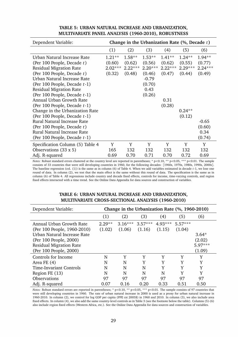
TABLE 5: URBAN NATURAL INCREASE AND URBANIZATION,MULTIVARIATE PANEL ANALYSIS (1960-2010), ROBUSTNESS

Dependent Variable: Change in the Urbanization Rate (%, Decade t)

(1) (2) (3) (4) (5) (6)

Urban Natural Increase Rate 1.21** 1.58** 1.53** 1.41** 1.24** 1.94**(Per 100 People, Decade t) (0.60) (0.62) (0.56) (0.62) (0.55) (0.77)Residual Migration Rate 2.02*** 2.22*** 2.20*** 2.22*** 2.29*** 2.24***(Per 100 People, Decade t) (0.32) (0.48) (0.46) (0.47) (0.44) (0.49)Urban Natural Increase Rate -0.79(Per 100 People, Decade t-1) (0.70)Residual Migration Rate 0.43(Per 100 People, Decade t-1) (0.26)Annual Urban Growth Rate 0.31(Per 100 People, Decade t-1) (0.28)Change in the Urbanization Rate 0.24**(Per 100 People, Decade t-1) (0.12)Rural Natural Increase Rate -0.65(Per 100 People, Decade t) (0.60)Rural Natural Increase Rate 0.34(Per 100 People, Decade t-1) (0.74)

Specification Column (5) Table 4 Y Y Y Y Y YObservations (33 x 5) 165 132 132 132 132 132Adj. R-squared 0.69 0.70 0.71 0.70 0.72 0.69Notes: Robust standard errors clustered at the country level are reported in parentheses; * p<0.10, ** p<0.05, *** p<0.01. The sampleconsists of 33 countries that were still developing countries in 1960, for the following decades: [1960s, 1970s, 1980s, 1990s, 2000s].The baseline regression (col. (1)) is the same as in column (6) of Table 4. When we add variables estimated in decade t-1, we lose oneround of data. In column (2), we test that the main effect is the same without this round of data. The specification is the same as incolumn (6) of Table 4. All regressions include country and decade fixed effects, controls for income, time-varying controls, and regionfixed effects interacted with a time trend. See the Online Data Appendix for data sources and construction of variables.

TABLE 6: URBAN NATURAL INCREASE AND URBANIZATION,MULTIVARIATE CROSS-SECTIONAL ANALYSIS (1960-2010)

Dependent Variable: Change in the Urbanization Rate (%, 1960-2010)

(1) (2) (3) (4) (5) (6)

Annual Urban Growth Rate 2.29** 3.16*** 3.57*** 4.93*** 5.57***(Per 100 People, 1960-2010) (1.02) (1.06) (1.16) (1.15) (1.04)Urban Natural Increase Rate 3.64*(Per 100 People, 2000) (2.02)Residual Migration Rate 5.97***(Per 100 People, 2000) (1.09)Controls for Income N Y Y Y Y YArea FE (4) N N Y Y Y YTime-Invariant Controls N N N Y Y YRegion FE (13) N N N N Y YObservations 97 97 97 97 97 97Adj. R-squared 0.07 0.16 0.20 0.33 0.51 0.50Notes: Robust standard errors are reported in parentheses; * p<0.10, ** p<0.05, *** p<0.01. The sample consists of 97 countries thatwere still developing countries in 1960. The rate of urban natural increase in 2000 is used as a proxy for urban natural increase in1960-2010. In column (2), we control for log GDP per capita (PPP, cst 2005$) in 1960 and 2010. In column (3), we also include areafixed effects. In column (4), we also add the same country-level controls as in Table 3 (see the footnote below the table). Columns (5)-(6)also include region fixed effects (Western Africa, etc.). See the Online Data Appendix for data sources and construction of variables.

29

TABLE 7: URBAN NATURAL INCREASE, URBAN GROWTH AND SLUMS (2000)MULTIVARIATE CROSS-SECTIONAL ANALYSIS (1960-2010)

Dependent Variable: Urban Population Living in Slums (%, 2005)

(1) (2) (3) (4) (5) (6) (7) (8)

Annual Urban Growth Rate 8.93***4.39***3.83** 6.52***6.43**(%, 1960-2010) (3.12) (1.26) (1.56) (2.27) (2.79)Change in Urbanization Rate -0.18 0.35** 0.35** 0.17 -0.00 0.05 0.06 0.10(%, 1960-2010) (0.29) (0.17) (0.17) (0.21) (0.28) (0.26) (0.22) (0.20)Number of Years in which the Urban Population Doubles -0.5*** -0.6***(Average, 1960-2010) (0.2) (0.2)Number of Years in which the Urban Population Doubles -0.7**(Average 1960-2010) * Dummy “Number of Years Below Mean” (0.3)Urban Natural Increase 14.44***(%, 2000) (5.01)Residual Migration 4.58*(%, 2000) (2.61)

Controls for Income N Y Y Y Y Y Y YArea FE (5) N N Y Y Y Y Y YTime-Invariant Controls N N Y Y Y Y Y YRegion FE (13) N N N N Y Y Y YObservations 95 95 95 95 95 95 95 95Adj. R-squared 0.17 0.61 0.62 0.67 0.68 0.70 0.69 0.70Notes: Robust standard errors are reported in parentheses; * p<0.10, ** p<0.05, *** p<0.01. The sample consists of 95 countries that werestill developing countries in 1960. The rate of urban natural increase in 2000 is used as a proxy for urban natural increase in 1960-2010. Theresidual migration rate is estimated as the difference between the annual urban growth rate in 1960-2010 and the rate of urban natural increasein 2000. The number of years in which the urban population doubles on average in 1960-2010 is estimated using the annual urban growth rate.We create a dummy variable equal to one if this number is below the mean in the sample (19.4). In column (2), we control for log GDP per capita(PPP, cst 2005$) in 1960 and 2010. In column (3), we also include area fixed effects. In column (4), we also add the same country-level controlsas in Table 3. Columns (5)-(8) also include region fixed effects. See the Online Data Appendix for data sources and construction of variables.

TABLE 8: URBAN NATURAL INCREASE AND MEASURES OF URBAN CONGESTIONMULTIVARIATE CROSS-SECTIONAL ANALYSIS (2000)

Dependent Variable: Lack Finished Access Access School PM10 EmplSufficient Floor Improved Improved Attend. (mg ShareLiving Water Sanitation (6-15 per Perso.Area Source Facilities y.o.) cubic Serv.(%) (%) (%) (%) (%) m) (%)

(1) (2) (3) (4) (5) (6) (7)

Urban Natural Increase 8.6* -6.5 -3.5** -1.2 −11.8*** 17.8* 4.0**(%, 2000) (4.6) (5.6) (1.6) (2.7) (3.9) (10.0) (2.0)

[0.46] [0.20] [0.21] [0.03] [0.49] [0.27] [0.49]Residual Migration 2.9 -1.3 -2.0* -2.0 -3.4 -0.0 1.2(%, 2000) (2.8) (3.6) (1.1) (1.9) (3.0) (5.7) (1.0)

[0.24] [0.07] [0.25] [0.11] [0.22] [0.00] [0.31]Specification Col. (8) Table 8 Y Y Y Y Y Y YSample Mean 18.8 77.9 89.5 65.1 80.2 71.3 5.5Observations 57 66 93 93 64 93 72Notes: Robust standard errors are reported in parentheses; * p<0.10, ** p<0.05, *** p<0.01. The effects of 1 standard deviation increase in thevariable of interest on 1 standard deviation in the dependent variable are reported in brackets. We regress various measures of urban congestionin 2000 on the rates of urban natural increase in 2000, which we use as a proxy for urban natural increase in 1960-2010. The residual migrationrate is estimated as the difference between the annual urban growth rate in 1960-2010 and the rate of urban natural increase in 2000. In column(1), the dependent variable is the share of urban inhabitants who lack sufficient-living area (%), i.e. who live in dwelling units with more than 3persons per room. In column (2), it is the share of urban inhabitants who live in a residence with a finished floor (%). In columns (3) and (4), itis the share of urban inhabitants who have access to an improved water source and improved sanitation facilities respectively (%). In column (5),it is the urban share of 6-15 year-old children that attend school (%). In column (6), it is a measure of particulate matter (PM) concentrations inresidential areas of cities with more than 100,000 residents. In column (7), it is the urban employment share of personal and other services (%),an informal refugee sector. The specification is the same as in column (8) of Table 7. All regressions include controls for income, time-invariantcontrols, and region fixed effects. See the Online Data Appendix for data sources and construction of variables.

Figure 1: Urbanization Rates (%) for Europe (1700-1950)and The Developing World (1900-2010)

Notes: This figure plots the urbanization rate (%) for Europe (1700-1950) and four developingregions (1900-2010): Africa, Asia, Latin America and the Caribbean (LAC) and Middle-East andNorth Africa (MENA). Europe includes 18 Western European countries and the United States, asone example of a Neo-European country. We then use data for 116 African, Asian and non-NorthAmerican countries that were still developing countries in 1960. Averages are estimated using thepopulation weights for the same year. See the Online Data Appendix for data sources.

Figure 2: Annual Urban Growth Rates (%) for Europe (1700-1950)and The Developing World (1900-2010)

Notes: This figure plots the annual urban growth rate (%) for Europe (1700-1950) and four devel-oping regions (1900-2010): Africa, Asia, Latin America and the Caribbean (LAC) and Middle-Eastand North Africa (MENA). Europe includes 18 Western European countries and the United States,as one example of a Neo-European country. We then use data for 116 African, Asian and non-NorthAmerican countries that were still developing countries in 1960. Averages are estimated using thepopulation weights for the same year. See the Online Data Appendix for data sources.

31

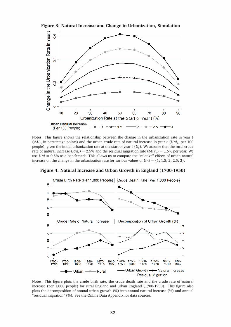
Figure 3: Natural Increase and Change in Urbanization, Simulation

Notes: This figure shows the relationship between the change in the urbanization rate in year t(∆Ut , in percentage points) and the urban crude rate of natural increase in year t (Unit , per 100people), given the initial urbanization rate at the start of year t (Ut). We assume that the rural cruderate of natural increase (Rnit) = 2.5% and the residual migration rate (Migt) = 1.5% per year. Weuse Uni = 0.5% as a benchmark. This allows us to compare the “relative” effects of urban naturalincrease on the change in the urbanization rate for various values of Uni = {1; 1.5; 2; 2.5; 3}.

Figure 4: Natural Increase and Urban Growth in England (1700-1950)

Notes: This figure plots the crude birth rate, the crude death rate and the crude rate of naturalincrease (per 1,000 people) for rural England and urban England (1700-1950). This figure alsoplots the decomposition of annual urban growth (%) into annual natural increase (%) and annual“residual migration” (%). See the Online Data Appendix for data sources.

32

Figure 5: Crude Birth Rates for The Developing World (1960-2010)

Notes: This figure plots the crude birth rate (per 1,000 people) for the rural and urban areas of fourdeveloping regions (1960-2010): Africa, Asia, Latin America and the Caribbean (LAC) and Middle-East and North Africa (MENA). We use demographic data that we have collected for 33 countriesthat were still developing countries in 1960. See the Online Data Appendix for data sources.

Figure 6: Crude Death Rates for The Developing World (1960-2010)

Notes: This figure plots the crude death rate (per 1,000 people) for the rural and urban areas of fourdeveloping regions (1960-2010): Africa, Asia, Latin America and the Caribbean (LAC) and Middle-East and North Africa (MENA). We use demographic data that we have collected for 33 countriesthat were still developing countries in 1960. See the Online Data Appendix for data sources.

33

Figure 7: Crude Rates of Natural Increase for The Developing World (1960-2010)

Notes: This figure plots the crude rate of natural increase (per 1,000 people) for the rural and urbanareas of the four developing areas (1960-2010). We use historical demographic data for 33 countriesthat were still developing countries in 1960. See the Online Data Appendix for data sources.

Figure 8: Natural Increase and Urban Growthfor The Two Developing Worlds (1700-1950 and 1960-2010)

Notes: This figure plots the decomposition of annual urban growth (%) into annual natural increase(%) and annual “residual migration” (%) for the four developing areas, the developing world as awhole in 1960-2010 and England in 1700-1950. We use historical demographic data for 33 countriesthat were still developing countries in 1960. See the Online Data Appendix for data sources.

34

FOR ONLINE PUBLICATION: DATA SOURCES

This appendix describes in details the data we use in our analysis.

Spatial Units for Industrial Europe and Today’s Developing World:We use three different samples in our analysis. First, we obtain historical urban data for19 European and North American countries from 1700-1950, and 116 Africa, Asian or non-North American countries that were still developing countries in 1960, from 1960-2010. Weexclude from our analysis the European countries for which we could not find historicallyconsistent urban data, as well as the former CIS countries. We use these countries to de-scribe urban patterns in “Industrial Europe” (which also includes a Neo-European country,the United States) and four developing areas: Sub-Saharan Africa (which we call “Africa”),Asia, Latin America and the Caribbean (LAC), and Middle-East and North Africa (MENA).Second, our main sample consists of 40 of these countries from 1700 to 2010. These arethe countries for which we found historical demographic data. Historical consistent datawas not found for other countries. The list of countries and years (or periods) for whichwe have data is reported in Appendix Tables 1, 2 and 3. These countries belong to the fivedeveloping areas: Industrial Europe (N = 7, about every 40 years in 1700-2010), Africa (N= 10, every ten years in 1960-2010), Asia (N = 11, ditto), LAC (N = 8, ditto) and MENA(N = 4, ditto). Third, we also collect cross-sectional data for 97 out of the 116 countriesfor which we were to able to find demographic data, for the most recent period. The coun-tries of Africa, Asia, the LAC and MENA regions are then classified into 13 regions: CentralAfrica, Eastern Africa and Western Africa for Africa; East Asia, Pacific Islands, South Asiaand South-East Asia for Asia; Caribbean, Central America and South America for the LACregion; and Middle-East and North Africa for the MENA region.

Urban Growth and Urbanization in Industrial Europe:The annual urban growth rate is the average growth rate of the urban population betweentwo years (%). The urbanization rate is defined as the share of the urban population in totalpopulation (%). We use Bairoch (1988) and Malanima and Volckart (2007) to reconstructconsistent urban growth and urbanization rates for 18 Western European countries and theUnited States for the following periods: 1700-1750, 1750-1800, 1800-1850, 1850-1910and 1910-1950. Averages are estimated using the population weights for the same period.We then consider 7 countries in our main analysis (listed in Appendix Table 1). We alsouse Bairoch (1988), Batou and Chevre (1988) and Wikipedia (2013) to obtain the annualgrowth rate of the largest city for the 19 countries for each period.

Urban Growth and Urbanization in Today’s Developing World:We reference Bairoch (1988), Sluglett (2008) and WUP (2011) to reconstruct the urbangrowth and urbanization rates for Africa, Asia and the LAC and MENA regions for the fol-lowing periods: 1900-1920, 1920-1930, 1930-1950, 1950-1960, 1960-1970, 1970-1980,1980-1990, 1990-2000 and 2000-2010. For the last six decades, we use data for 116African, Asian and non-North American countries from 1950-2010. Averages are estimatedusing the population weights for the same period. We consider 33 countries in the panelanalysis from 1960-2010 (listed in Appendix Table 2). We then consider 97 out of the 116countries for the cross-sectional analysis from 1960-2010. We also use WUP (2011) andWB (2013) to estimate the growth rate of the largest city for each country, for the followingperiods: 1960-1970, 1970-1980, 1980-1990, 1990-2000 and 2000-2010.

Urban Demographic Transition in Industrial Europe:For each of the 7 countries of Industrial Europe, we use various historical sources to obtainthe national, urban and rural crude rates of birth, crude rates of death and crude ratesof natural increase (per 1,000 people) for several decades during the 1800-1910 period(sources listed in Panel A, Appendix Table 3). For England, our main European country of

A. 1

analysis, we have data from 1700 to 1950. For the six other countries, demographic dataonly exists for shorter periods.

Urban Demographic Transition in Today’s Developing World:For each of the 33 countries of today’s developing world, we use reports from the Populationand Housing Censuses, CICRED Monographs, Fertility Surveys, and Demographic and HealthSurveys (DHS) as well as the Statistical Yearbooks of the United Nations, to obtain the na-tional, urban and rural crude rates of birth, crude rates of death and crude rates of naturalincrease (per 1,000 people) for each decade during the 1960-2010 period (sources listed inPanel B, Appendix Table 3). We could not find consistent historical data for other countries.Indeed, demographic data does not always exist for countries as far back as the 1960s. For64 other countries of today’s developing world, we use reports from the Population andHousing Censuses and Demographic and Health Surveys to obtain an estimate of the urbanand rural crude rates of birth and death for the closest year to 2000, in the 1990-2010interval. For the 33 + 64 = 97 countries, we also used the same sources to retrieve theurban fertility rate for the closest year to 2000, in the 1990-2010 interval. For 94 countriesof today’s developing world, we also use the sources mentioned above to obtain the birthrate of the largest city for the closest year to 2000, in the 1990-2010 interval. Data on thecrude death rate of the largest city does not exist.

Measures of Urban Congestion:Data on the share of the urban population living in slums (%) comes from UN-Habitat(2003), UN (2013) and WB (2013). A slum household is usually defined as a group ofindividuals living under the same roof lacking one or more of the following conditions (UN-Habitat 2003): (i) sufficient-living area, (ii) structural quality, (iii) access to improved watersource, and (iv) access to improved sanitation facilities. We have data for 113 countries,but we focus on 95 countries for which we also have data on urban natural increase in2000. Data is available for a lower number of countries for some subcomponents of theslum variable. UN-Habitat (2003) reports the share of urban residents that lack “sufficient-living area”, i.e. who live in dwelling units with more than 3 persons per room. We useas a measure of “structural quality” the share of urban inhabitants who live in a residencewith a finished floor. We reconstruct this variable using the International Public-Use Micro-data Series (IPUMS, 2013) and the stat compiler of the Demographic and Health Surveys(DHS, 2013). Data on the share of urban inhabitants who have access to an improved wa-ter source and improved sanitation facilities (%) comes from WB (2013). A household isconsidered to have access to an improved water source if it has sufficient amount of wa-ter for family use, at an affordable price, available to household members without beingsubject to extreme effort, especially to women and children. A household is considered tohave access to improved sanitation, if an excreta disposal system is available to householdmembers. Data on the urban share of 6-15 year-old children that attend school (%) comesfrom the DHS (2013) and IPUMS (2013). Data on our measure of particulate matter (PM)concentrations in residential areas of cities with more than 100,000 residents comes fromWB (2013).

Urban Employment:Data on the urban employment structure in selected countries for 2000-2010 was recreatedusing various sources, as described for each country in Gollin, Jedwab and Vollrath (2013).We use five different sources of data. Our two main data sources are IPUMS (2013), theInternational Public-Use Microdata Series, and ILO (2013), the International Organizationof Labor. We complement these datasets with data from the published reports of Popula-tion and Housing Censuses, Labor Force Surveys and Household Surveys. For each country forwhich data is available, we estimate the employment shares of all urban areas for the follow-ing 11 sectors: “agriculture”, “mining”, “public utilities”, “manufacturing”, “construction”,“wholesale and retail trade, hotels and restaurants”, “transportation, storage and commu-

A. 2

nications”, “finance, insurance, real estate and business services”, “government services”,“education and health” and “personal and other services”.

Income and Other Controls:We have GDP per capita every ten years for 1960-2010. The main variable used in ouranalysis is average log GDP per capita for each decade (constant 2005 international $). Weuse various sources to reconstruct a range of time-invariant or time-varying controls at thecountry-level. In the panel regressions, we include the time-varying controls (estimated inthe same or previous decade). In the cross-sectional regressions, we also include the time-invariant controls (the time-varying controls are estimated for 1960-2010 instead of for thesame or previous decade).

First, we consider various rural push factors: (i) FAO (2013) reports the cereal yields (hg perha) for each country-year observation. We then estimate the average yields for each decade;(ii) Rural density is defined as the ratio of rural population (1000s) to arable area (sq km).The arable area of each country is reported by FAO (2013); (iii) CRED (2013) reports thenumber of droughts experienced by each country every year. We use two variables: thenumber of droughts (per sq km) since 1960, and the number of droughts (per sq km) foreach decade (e.g., 1960-1969 for the 1960s); and (iv) The Polity IV data series includes ameasure of political violence for each country (1964-present). We create an indicator whosevalue is one if the country experienced an interstate or civil conflict in each decade (PolityIV 2013a).

Second, we consider various urban pull factors: (i) The share of manufacturing and servicesin GDP (%) in 2010 is obtained from WB (2013). The data is missing for many country-year observations before the recent period; (ii) We use the data set of Gollin, Jedwab andVollrath (2013) to obtain the average share of natural resource exports in GDP (%) for eachdecade; (iii) We use the Polity IV data series to calculate the average combined polity scorefor each country for each decade (Polity IV 2013b). We create an indicator whose valueis one if the average polity score is lower than -5, the threshold for not being consideredautocratic; and (iv) From WB (2013), we know the share of the largest city in the urbanpopulation, the primacy rate, for all years in 1960-2010.

Third, we use the other following controls: (i) The 97 countries use four different types ofurban definition in their most recent censuses: (a) “administrative cities” are administra-tive centers of territorial units (e.g., provinces, districts, “communes”, etc.), (b) “thresholdcities” are localities whose population is greater than a population threshold of X inhabitants(e.g.,5,000 or 2,500), (c) “administrative or threshold cities” are either administrative cen-ters or localities whose population is greater than a population threshold, and (d) “thresholdwith condition cities” are localities whose population is greater than a population thresholdand who have a large share of the labor force is engaged in non-agricultural activities. Wecreate indicator variables for each definition. For each country using a population threshold,we know the threshold and use it as a control in our regression analysis; (ii) WUP (2011)reports total population for each country every year for 1950-2010; (iii) Country area (sqkm) is obtained from WB (2013); and (iv) We create two indicators whose value is one ifthe country is a small island or if the country is landlocked. We consider an island country“small” if its area is smaller than 50,000 sq km.

REFERENCES

Bairoch, Paul. 1988. Cities and Economic Development: From the Dawn of History to thePresent. Chicago: The University of Chicago Press.

Bairoch, Paul, Batou, Jean, and Pierre Chevre. 1988 Population des villes européennes de 800à 1850 : banque de données et analyse sommaire des résultats. Geneva: Librairie Doz.

A. 3

CRED. 2013. EM-DAT: International Disaster Database Louvain: Centre for Research on theEpidemiology of Disasters (CRED), Université Catholique de Louvain.

DHS. 2013. Demographic and Health Surveys. Washington, DC: USAID.

FAO. 2013. FAOSTAT. Roma: Food and Agriculture Organization.

Gollin, Jedwab and Vollrath (2013). Urbanization with and without Industrialization. Un-published manuscript, Department of International Development, University of Oxford.

ILO. 2013. ILOSTAT Database. Roma: International Labor Organization.

IPUMS. 2013. Integrated Public-Use Microdata Series, International. Minneapolis, MN: Min-nesota Population Center.

Malanima, Paolo, and Oliver Volckart. 2007. Urbanisation 1700-1780. Chapter preparedfor the Third RTN/CEPR Summer Symposium in London: An Economic History of ModernEurope.

Polity IV. 2013a. Polity IV Project: Political Regime Characteristics and Transitions, 1800-2011: Polity IV Annual Time-Series 1800-2011. Vienna: Center for Systemic Peace.

Polity IV. 2013b. Polity IV Project: Political Regime Characteristics and Transitions, 1800-2011: Major Episodes of Political Violence, 1946-2011. Vienna: Center for Systemic Peace.

Sluglett, Peter. 2008. The Urban Social History of the Middle East: 1750-1950. Syracuse:Syracuse University Press.

UN. 2013. Millenium Development Goals Indicators. New York: United Nations.

WB. 2013. World Development Indicators. Washington, DC: World Bank.

Wikipedia. 2013. City of X, in the United States, Economy of Country X, Landlocked country,Largest Cities of Country X and List of Island Countries. San Francisco, CA: Wikipedia.

WUP. 2011. World Urbanization Prospects, the 2011 Revision. New York: United Nations.

A. 4

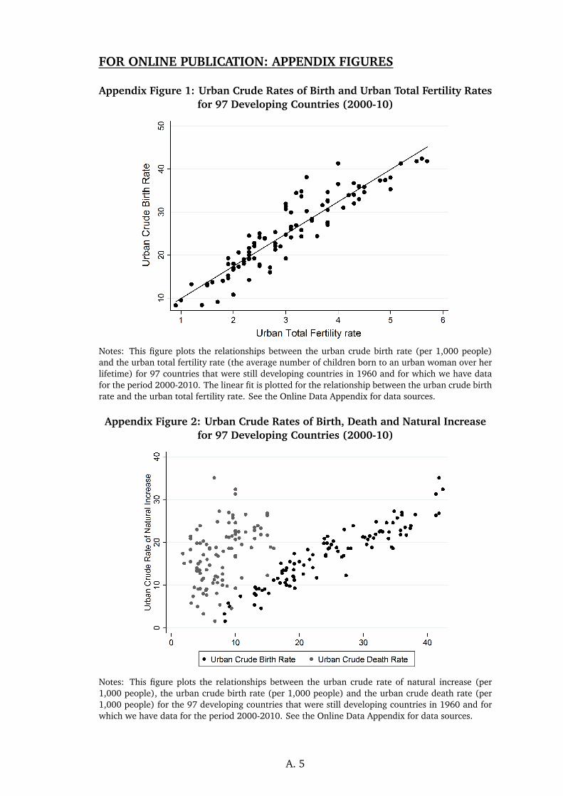
FOR ONLINE PUBLICATION: APPENDIX FIGURES

Appendix Figure 1: Urban Crude Rates of Birth and Urban Total Fertility Ratesfor 97 Developing Countries (2000-10)

Notes: This figure plots the relationships between the urban crude birth rate (per 1,000 people)and the urban total fertility rate (the average number of children born to an urban woman over herlifetime) for 97 countries that were still developing countries in 1960 and for which we have datafor the period 2000-2010. The linear fit is plotted for the relationship between the urban crude birthrate and the urban total fertility rate. See the Online Data Appendix for data sources.

Appendix Figure 2: Urban Crude Rates of Birth, Death and Natural Increasefor 97 Developing Countries (2000-10)

Notes: This figure plots the relationships between the urban crude rate of natural increase (per1,000 people), the urban crude birth rate (per 1,000 people) and the urban crude death rate (per1,000 people) for the 97 developing countries that were still developing countries in 1960 and forwhich we have data for the period 2000-2010. See the Online Data Appendix for data sources.

A. 5

FOR ONLINE PUBLICATION: APPENDIX TABLES

Appendix Table 1: Decomposition of Annual Urban Growthfor 7 European Countries, 1800-1910

Country Period: 1800-1850 1850-1870 1870-1910 1800-1910

EnglandUrban Growth (%) 2.7 1.8 2.2 2.3Natural Increase (%) 0.0 0.5 1.1 0.5Residual Migration (%) 2.7 1.3 1.1 1.9

BelgiumUrban Growth (%) 1.9 0.3 2.5 1.8Natural Increase (%) _ 0.4 0.6 0.5Residual Migration (%) _ -0.1 1.9 1.3

FranceUrban Growth (%) 1.3 1.0 1.5 1.3Natural Increase (%) _ 0.2 0.1 0.1Residual Migration (%) _ 0.7 1.4 1.2

GermanyUrban Growth (%) 1.8 3.0 3.0 2.5Natural Increase (%) 0.1 0.2 1.0 0.6Residual Migration (%) 1.7 2.8 2.0 1.9

NetherlandsUrban Growth (%) 0.9 0.7 2.1 1.3Natural Increase (%) 0.0 0.5 1.2 0.4Residual Migration (%) 0.9 0.2 0.9 0.9

SwedenUrban Growth (%) 0.8 2.0 3.2 1.9Natural Increase (%) -0.5 0.5 1.0 0.3Residual Migration (%) 1.3 1.5 2.2 1.6

United StatesUrban Growth (%) 5.2 5.7 3.5 4.6Natural Increase (%) 0.3 0.4 0.4 0.4Residual Migration (%) 4.8 5.3 3.1 4.3

AverageUrban Growth (%) 2.1 2.1 2.6 2.2Natural Increase (%) 0.0 0.4 0.7 0.5Residual Migration (%) 2.1 1.7 1.8 1.7

Notes: This table shows the decomposition of annual urban growth into annual natural increase andannual residual migration (%) for 6 European countries and one Neo-European country, the UnitedStates (1800-1910). Averages are not weighted by population. See the Online Data Appendix fordata sources.

A. 6

Appendix Table 2: Decomposition of Annual Urban Growthfor 33 Developing Countries, 1960-2010

Period: 1960-2010 2000-2010

Subregion Country UrbanGrowth

NaturalIncr.

ResidualMigr.

UrbanGrowth

NaturalIncr.

ResidualMigr.

ASIA 3.5 1.7 1.8 2.3 1.1 1.2

East Asia (N = 3): 2.9 1.1 1.8 2.0 0.4 1.6East Asia China 3.7 1.0 2.7 3.8 0.8 3.0East Asia Japan 1.4 0.7 0.7 1.5 0.0 1.5East Asia South Korea 3.6 1.5 2.1 0.9 0.5 0.3South Asia (N = 4): 3.5 1.9 1.6 2.3 1.4 0.9South Asia Bangladesh 5.8 2.1 3.7 3.1 1.1 2.0South Asia India 3.2 1.8 1.4 2.6 1.3 1.3South Asia Pakistan 3.7 2.2 1.5 2.7 1.9 0.8South Asia Sri Lanka 1.3 1.5 -0.2 0.6 1.1 -0.5Southeast Asia (N = 4): 3.9 1.9 2.0 2.5 1.4 1.2Southeast Asia Indonesia 4.5 1.8 2.7 2.9 1.6 1.3Southeast Asia Malaysia 4.6 2.1 2.5 3.5 1.4 2.1Southeast Asia Philippines 3.6 2.4 1.2 2.0 2.1 -0.1Southeast Asia Thailand 3.0 1.4 1.6 1.7 0.4 1.3

LAC 3.1 2.2 0.9 2.1 1.5 0.6

Central America (N = 4): 3.2 2.5 0.7 2.4 1.7 0.7Central America El Salvador 2.7 2.5 0.2 1.3 1.2 0.1Central America Guatemala 3.5 2.8 0.7 3.4 2.8 0.6Central America Mexico 3.1 2.5 0.6 1.7 1.2 0.5Central America Panama 3.5 2.3 1.2 3.0 1.5 1.5South America (N = 4): 3.1 2.0 1.1 1.9 1.3 0.6South America Chile 2.2 1.7 0.5 1.4 1.0 0.4South America Colombia 3.2 1.9 1.3 1.9 1.7 0.3South America Ecuador 3.8 1.9 1.9 2.7 1.1 1.6South America Peru 3.2 2.4 0.8 1.7 1.5 0.2

MENA 3.6 2.6 1.0 2.1 1.6 0.5

Middle-East (N = 2): 4.5 2.8 1.6 2.4 1.8 0.6Middle-East Iran 3.9 2.6 1.3 2.0 1.3 0.7Middle-East Jordan 5.0 3.0 1.9 2.9 2.4 0.4Northern Africa (N = 2): 2.7 2.3 0.4 1.7 1.3 0.4Northern Africa Egypt 2.4 2.2 0.2 2.0 1.7 0.3Northern Africa Tunisia 3.0 2.4 0.6 1.5 0.9 0.5

AFRICA 4.9 2.9 2.1 4.1 2.4 1.7

Eastern Africa (N = 5): 4.9 2.8 2.1 3.7 2.2 1.4Eastern Africa Central Afr. Rep.* 3.5 2.4 1.1 2.1 2.0 0.1Eastern Africa Ethiopia 4.6 2.7 1.9 3.8 2.0 1.7Eastern Africa Kenya 5.7 2.8 2.9 4.4 2.4 2.0Eastern Africa Madagascar 5.1 2.5 2.6 4.7 2.3 2.5Eastern Africa Malawi 5.6 3.7 1.9 3.5 2.6 0.9Western Africa (N = 5): 4.9 2.9 2.0 4.5 2.6 1.9Western Africa Burkina-Faso 6.0 3.0 3.0 6.8 3.1 3.7Western Africa Ghana 4.2 2.5 1.8 4.0 1.8 2.2Western Africa Ivory Coast 5.7 2.7 3.0 3.3 2.4 1.0Western Africa Mali 4.5 3.4 1.1 5.2 3.5 1.7Western Africa Senegal 4.1 2.8 1.4 3.2 2.5 0.8

All Countries 3.8 2.3 1.6 2.8 1.7 1.1

Notes: This table shows the decomposition of annual urban growth into annual natural increase andannual residual migration (%) for 33 developing countries (1960-2010). * The Central African Republicbelongs to Central Africa, but data is missing for other countries of the region. We have included it inEastern Africa. Averages are not weighted by population. See the Online Data Appendix for data sources.

A. 7

Appendix Table 3: Natural Increase Source Information by Country

Panel A: Historical Data for Industrial Europe (1800-1910)

Country Region Years Main Sources

Belgium Europe 1866-1905 Annuaires Statistiques de la Belgique. Belgium. Ministere del’Interieur. Various volumes.

England Europe 1700-1950 Newsholme, A. (1911), The Declining Birth Rate, Its Nationaland International Significance. London: Cassell & CompanyLimited.Friedlander, D. (1969). Demographic Responses and PopulationChange, Demography 6 (4): 359-381.Williamson, J. (1990). Coping with City Growth During theBritish Industrial Revolution. Cambridge: Cambridge UniversityPress.

France Europe 1852-1910 Statistique Annuelle du Mouvement de la Population. France.Statistique Generale. Various volumes.

Germany Europe 1851-1912 Weber, A. (1899). The Growth of Cities in the 19th Century. NewYork: The MacMillan Company.Stedman, T. (1904). Medical Record. New York: William Woodand Company.Pollock, H., and W. Morgan (1913). Modern Cities: Progress ofthe Awakening for Their Betterment Here and in Europe. NewYork: Funk & Wagnalls Company.Holmes, S. (1921). A Study of Present Tendencies in the BiologicalDevelopment of Civilized Mankind. New York: Harcourt, Braceand Company.Vogele, J. (2000). Urbanization and the urban mortality changein Imperial Germany. Health & Place 6: 41-55.

Netherlands Europe 1815-1909 Margaret Sanger (1917). The Case for Birth Control. Modern ArtPrinting Company.Wintle, M. (2004). An Economic and social History of theNetherlands, 1800-1920: Demographic, Economic and SocialTransition. Cambridge: Cambridge University Press.

Sweden Europe 1800-1910 Dyson, T. (2011), The Role of the Demographic Transition in theProcess of Urbanization. Population and Development Review, 37:34-54.

United States Europe 1825-1910 Various Census Reports.Duffy J. (1968). A History of Public Health in New York City,1625-1866. New York: Russell Sage.Rosenwaike, I. (1972). Population History of New York City.Syracuse: Syracuse University Press.Haines, M. (2001). The Urban Mortality Transition in the UnitedStates, 1800-1940. Annales de Demographie Historique 101:33-64.Michael R. Haines, The Population of the United States,1790-1920. Cambridge: Cambridge University Press, 2008.Ferrie, J.P., and W. Troesken (2008). Death and The City:Chicago’s Mortality Transition, 1850-1925. Explorations inEconomic History, 45, 1: 1-16.

A. 8

Appendix Table 3: Natural Increase Source Information by Country

Panel B: Historical Data for Developing Countries (1960-2010)

Country Region Years Main Sources

Bangladesh Asia 1965, 1974, 1985,1991, 2004

UN Statistical Yearbook, Population and Housing Census(Report), Demographic and Health Survey (Report),CICRED Monograph

Burkina Faso Africa 1960, 1975, 1985,1996, 2006

Population and Housing Census (Report), Demographicand Health Survey (Report)

Central Afr. Rep. Africa 1960, 1975, 1988,1994-1995, 2003

Population and Housing Census (Report), Demographicand Health Survey (Report), Fertility Survey (Report)

Chile LAC 1960, 1970, 1983,1995, 2006

UN Statistical Yearbook, Population and Housing Census(Report), CICRED Monograph

China Asia 1965, 1975, 1985,1995, 2000

UN Statistical Yearbook, Population and Housing Census(Report), CICRED Monograph

Colombia LAC 1965, 1973, 1985,1990, 2000

UN Statistical Yearbook, Population and Housing Census(Report), Demographic and Health Survey (Report),CICRED Monograph

Côte d’Ivoire Africa 1965, 1975, 1988,1994, 1999

Population and Housing Census (Report), Demographicand Health Survey (Report), Fertility Survey (Report)

Ecuador LAC 1968, 1974, 1985,1993, 2005

UN Statistical Yearbook, Population and Housing Census(Report), Demographic and Health Survey (Report)

Egypt MENA 1962, 1975, 1985,1996, 2006

UN Statistical Yearbook, Population and Housing Census(Report), Demographic and Health Survey (Report),CICRED Monograph

El Salvador LAC 1965, 1975, 1985,1996, 2006

UN Statistical Yearbook, Population and Housing Census(Report), Demographic and Health Survey (Report)

Ethiopia Africa 1967, 1974, 1984,1994, 2000

Population and Housing Census (Report), Demographicand Health Survey (Report), Fertility Survey (Report)

Ghana Africa 1960, 1970, 1984,1992, 2000

Population and Housing Census (Report), Demographicand Health Survey (Report), CICRED Monograph

Guatemala LAC 1965, 1975, 1980,1992, 1999

UN Statistical Yearbook, Population and Housing Census(Report), Demographic and Health Survey (Report)

India Asia 1961, 1970, 1985,1989, 2005

UN Statistical Yearbook, Population and Housing Census(Report), Demographic and Health Survey (Report),CICRED Monograph

Indonesia Asia 1961, 1975, 1985,1993, 2003

UN Statistical Yearbook, Population and Housing Census(Report), Demographic and Health Survey (Report),CICRED Monograph

Iran MENA 1968, 1975, 1986,1990, 2005

UN Statistical Yearbook, Population and Housing Census(Report), CICRED Monograph

Japan Asia 1965, 1975, 1985,1995, 2005

UN Statistical Yearbook, Population and Housing Census(Report), CICRED Monograph

Jordan MENA 1965, 1973, 1990,1997, 2002

UN Statistical Yearbook, Population and Housing Census(Report), Demographic and Health Survey (Report)

Kenya Africa 1962, 1969, 1979,1989, 1999

Population and Housing Census (Report), Demographicand Health Survey (Report), Fertility Survey (Report),CICRED Monograph

A. 9

Country Region Years Main Sources

Madagascar Africa 1965, 1975, 1985,1993, 2000

Population and Housing Census (Report), Demographicand Health Survey (Report), Fertility Survey (Report)

Malawi Africa 1970, 1977, 1987,1998, 2008

Population and Housing Census (Report), Demographicand Health Survey (Report), Fertility Survey (Report)

Malaysia Asia 1960, 1970, 1980,1990, 2006

UN Statistical Yearbook, Population and Housing Census(Report), CICRED Monograph

Mali Africa 1960, 1976, 1987,1998, 2006

Population and Housing Census (Report), Demographicand Health Survey (Report), Fertility Survey (Report)

Mexico LAC 1965, 1974, 1980,1990, 2006

UN Statistical Yearbook, Population and Housing Census(Report), Demographic and Health Survey (Report)

Pakistan Asia 1968, 1971, 1984,1988, 2000

UN Statistical Yearbook, Population and Housing Census(Report), Demographic and Health Survey (Report),CICRED Monograph

Panama LAC 1965, 1969, 1985,1995, 2006

UN Statistical Yearbook, Population and Housing Census(Report), CICRED Monograph

Peru LAC 1960, 1970, 1986,1990, 2000

Population and Housing Census (Report), Demographicand Health Survey (Report), Fertility Survey (Report),CICRED Monograph

Philippines Asia 1968, 1978, 1988,1998, 2003

UN Statistical Yearbook, Population and Housing Census(Report), Demographic and Health Survey (Report),CICRED Monograph

Senegal Africa 1960, 1976, 1988,1993, 2002

Population and Housing Census (Report), Demographicand Health Survey (Report), Fertility Survey (Report)

South Korea Asia 1960, 1966, 1970,1989, 2006

UN Statistical Yearbook, Population and Housing Census(Report), CICRED Monograph

Sri Lanka Asia 1961, 1971, 1983,1987, 2001

UN Statistical Yearbook, Population and Housing Census(Report), Demographic and Health Survey (Report),CICRED Monograph

Thailand Asia 1965, 1975, 1985,1995, 2005

UN Statistical Yearbook, Population and Housing Census(Report), Demographic and Health Survey (Report),CICRED Monograph

Tunisia MENA 1966, 1972, 1980,1989, 2005

UN Statistical Yearbook, Population and Housing Census(Report), Demographic and Health Survey (Report),CICRED Monograph

A. 10