322

Rural Areas in the Czech Republic: How Do They Differ from Urban Areas?

–

–

Annotation: There has been wide discussion among researchers, policy-makers and various rural stakeholders about the special position of rural areas. It is argued that rural areas are subject of various problems and deserve special attention and financial support. The aim of this article is to assess how the rural areas differ from the urban areas in certain features important for rural development. The basis for analysis is the current definition of rural areas according to the European Union on NUTS 3 level (analogy of “kraj” in the Czech Republic). The dataset from 2003 until 2011 includes 16 indicators from the area of population, economics, labour market, constructions, health and social security. The differences among values of particular indicator in predominantly rural (PR), intermediate (IN) and predominantly urban (PU) areas are tested using analysis of variance (ANOVA) method. When there are significant dissimilarities found, the particular means which differ from each other are tested using Tuckey’s test. According to our findings, we came to the conclusion that there are not statistically significant differences among PR, IN and PU shires in mortality, average living floor area per completed dwelling, healthcare indicators and average old-age person. On the other hand, there are statistically significant differences in other demographic features, economic characteristics and in labour market indicators. Therefore, the different situation of the PR areas might be a good argument justifying special attention and potential financial support.

Key words: rural areas, rural development, ANOVA, Tukey’s test, NUTS 3

JEL classification: C23, R11

1 Introduction

The rural areas must be defined especially for policy making purposes. There have been long debates among scholars and also at the policy making areas, whether the rural areas deserve special attitude and particularly financial support from the state or other institutions. Rural areas are considered to be different and being a subject of specific problems in various fields ranging from slower economic development, unfavorable demographic characteristics, higher rate of unemployment to difficult living conditions and remoteness. However, these expectations might not be true in all cases. We argue that rural areas are not always in poor situation in all indicators important for development. The article is structured as follows: firstly, the literature review of the main problems in rural areas in general and especially in relation to the CR in post-communism period is presented. Then the special approach towards rural areas is justified. The methodology and utilized statistical properties are described in the next chapter. The results are described on the basis of performed analysis of variance for the values of particular development indicators for the PR, IN and PU regions. Finally the conclusions are summarized.

323

Scholars devoted much time exploring the differences between “rural” and “urban” in the area of economic performance, demographic indicators, society characteristics, standards of living etc. However, according to Friedland (2002) “Whereas much of the definitional approach sought to find differences in socio-demographic, attitudinal, and cultural variables, an important finding was that rural and urban were less polarities or elements of a dichotomy than stations along a continuum.” „Researchers soon realized that there was no simple dichotomy between ‘rural’ and ‘urban’ areas. Instead, they recognized a variety of communities conforming to various levels of urbanism and ruralism” (Halfacree, 1993). As

gradually during the historical development and at present they are overlapping.”

Rural areas are subjects of specific problems. The situation was critical after the transitional period after the revolution in 1989 in the Czech Republic (CR). Tisenkopfs (1999) identified the problems of Latvia’s countryside in relation to the post-socialistic situation. He pointed out declined agricultural production, a scattered structure of enterprises, increased unemployment and poverty, poor infrastructure, great distances to cities, lack of business skills, low population density levels, the aging of the rural population and the weakness of non-governmental organizations. The situation in the CR was analogical. According to the

reduction of agricultural operations due to lack of competitiveness in comparison with original EU countries, loss of traditional employment opportunities, or worsening conditions for commuting.”

The situation in rural areas was influenced especially by changes in agriculture. „Over the past decades, major changes have taken place in Europe’s rural areas. These changes include contrasting developments like depopulation and land abandonment in some regions, and urbanisation and agricultural intensification in others.” (Westhoek et al., 2006, p. 7) In the CR strong collectivization during the socialist era had an impact on the current structure of the agricultural sector (Binek, Svobodová, 2009) as same as inadequate infrastructure, underdeveloped tertiary sector, low pay for workers employed in agriculture and lower availability of basic health and social services (Majerová 2003).

„Given the major political breakthrough represented by 1989 and membership in the EU in 2004, rural society in the Czech Republic has responded in variety of ways to the new requirements made by the marketplace and by EU directives in economic matters. Deep social and cultural changes, partly legitimated by national or EU projects and policies, have modified how Czech rural areas are used ... and how society views these areas.” (Chevalier, 2008)

In the strategic policy making documents of the Czech Republic are highlighted especially “population ageing, unfavorable age structure and low fertility levels, flight of the young, educated inhabitants and competent entrepreneurs, and low potential of economicdiversification are seen as the main threats.“ (Vobecká, 2009) According to the Rural Development Programme (RDP, Ministry of Agriculture, 2013), the major problem faced by rural areas is the stabilization of the rural population as it is aging more rapidly than the rest of the country because of the emigration of young people to urban centres to obtain jobs and better social infrastructure. Agriculture – with its relatively low share in the total employment (11 % in rural areas and 3.8 % overall) – has a 2011)

There are different approaches to solving the problems of rural areas, some of them acknowledging the role of the external financial support from the government. One extreme idea proclaims the state the main actor which has to solve the problems, because they are out

324

of reach of the local actors. The other one state that only market mechanism is able to come with solution for rural areas. (Surchev, 2010) There are even opinions that only development centres should be supported which can lead to the situation when „The development is concentrated in cities, while rural areas are falling ever farther behind.” (Tisenkopfs, 1999) Subsidiary principle introduced by the European Union can be seen reasonable compromise, where the decision-making power is given to the lowest level as possible. There is a bottom-up approach that the finances are distributed from the centre to the local authorities or actors. They are supposed to know the potential of their area and to better choose, what projects to implement to achieve the rural development. Berkel and Verburg (2011) are of the opinion that “targeting of the rural development policies on the areas with high potential can increase the effectiveness of the policies.” „Therefore it is important that new alternatives which are enabling to reflect the reality more suitably and overcome current, less optimal solutions are submitted, especially in the scientific area. In any case, it is necessary to take in account that none solution will be completely acceptable for all involved actors – due to the diversity of interests, missions and competences. However, this should not be irremovable barrier for knowledge and for development of the countryside and rural areas themselves.” (Binek et al., 2009).

2 Materials and Methods

Firstly, the rural areas were determined. New definition of the EU was used. It considers as rural areas the population living which is living outside the urban areas. These are determined as territories where the density of population is above 300 inhabitants per km2 applied to grid cell and a minimum size threshold (5,000 inhabitants) applied to grouped grid cells above the density threshold. (DG Agri, JRC, Eurostat, 2012) This approach has the benefit that it creates a more balanced distribution of population. In a number of countries the shifts between intermediate and predominantly rural are quite significant, as for example in the Czech Republic. (Eurostat, 2012) The analysis is applied on NUTS 3 regions (“kraj”) in the CR. The categorization of regions is displayed in Table 1.

Table 1. Indicators

Type of the region NUTS 3 region of the Czech RepublicPredominantly rural (PR)Intermediate (IN) Karlovarský, Ústecký, Liberecký, Královéhradecký,

Jihomoravský, Moravskoslezský

Predominantly urban (PU)

Secondly, relevant indicators related to the development potential of the rural regions were chosen on the bases of the literature review (Jánský, 2012, Margarian, 2013, Ministry of Rural

indicators from the area of population, economics, labour market, construction, health and social security were obtained from the public database of the Czech statistical office (CZSO). The Table 2 gives the overview. In the most of the cases, the data were available for the period 2003–2011.

325

Table 2. Indicators of the development

Area of indicators Indicator Units

Population

Mid-year population personsLive births per 1 000 population ‰Deaths per 1 000 population ‰Migration increase/decrease per 1 000 population ‰

EconomicsGross domestic product per capita CZKDisposable income of households per capita CZK

Area of indicators Indicator Units

Labour market (31 Dec)Registered unemployment rate %Job vacancies persons

Construction

Dwellings startedDwellings completedAverage living floor area per completed dwelling m2

Healthcare

Physicians in out-patient care establishments perpersons

1 000 population (FTE)Physicians in hospitals per 10 000 population (FTE) personsBeds in hospitals per 1 000 populationAverage incapacity for work %

Social security (31 Dec) Average old-age pension CZK

The approach towards the description of the differences is based on the statistical testing. Using analysis of variance (ANOVA, see e.g. Box, 1954-a or Cohen, 1988) it is tested whether the mean values of each indicator are statistically significantly different among PR, IN, PU regions. Values of particular indicator for each region for all years are grouped and considered to be one observation. Null hypothesis states that there is no statistically significant difference.

H0: 1 = 2 = 3 or (PR) = (IN) = (PU)

H1: non H0

The critical value of F-test is calculated and compared with the tabled value of the F-

hypothesis is rejected. There are statistically significant disparities. The same result can be seen also when comparing p- -value is lower

olds. Hence, there are statistically significance differences between at least two means. After this a Tukey’s test must be used in order to assess which two means significantly differ (see Mosteller, Tukey, 1977). Tukey’s test is

SE

YYq BA

s(1)

where YA is the larger of the two means being compared, YB is the smaller of the two means being compared, and SE is the standard error of the data in question. (Linton, Harder, 2007) The calculation table of the ANOVA is displayed in Table 3

326

Table 3. Computational scheme of ANOVA

Source Sum of Squares Df Mean Square F-ratio

Between groupi

k

i iby nyyS2

1, k-11

,2,

k

Ss

by

by

2,

2,

wy

by

s

sF

Within group 2

1 1,

k

i

n

j iijwy

i

yyS n-kkn

Ss

wy

wy

,2,

Total (Corr.)2

1 1

k

i

n

j ijy

i

yyS n-1

where k is the total number of factors (PR, IN, PU) and n is the total number of observations. The calculations are done in Statgraphics Centurion XVI and IBM SPSS Statistics.

3 Results and Discussion

Firstly, the regions of the Czech Republic were divided according to their affiliation to PR, IN or PU. The values of each indicator for all available years were assigned to particular group. The differences among the regions were consequently tested by one-way ANOVA.

Despite that rural areas are considered to have worst demographic characteristics, lower economic performance and worst state of infrastructure, the analysis showed that it is not true in all cases. The results showed that there are not statistically significant differences between means of the PR, IN and PU regions in case of deaths per 1 000 population, average living floor area per completed dwelling, physicians in out-patient care establishments per 1 000population, beds in hospitals per 1 000 population and average age-old pension. It means that all types of regions are similar in these areas and even PU does not do worst. As one indicator is from population group, one from construction area, one from social security and two from healthcare group, there is not clear pattern. It can be only stated that PU regions probably do not perform worst in the area of healthcare than PR or IN regions.

In case of the number of physicians and beds in hospitals, there are few significant outliers present. Nevertheless, they do not have impact on the results of the ANOVA due to the low variance of the values. In spite of that the results still show no statistical difference among the mean values. This can be clearly seen on Fig. 1 on Box and Whiskers plot (see e.g. McGill et al., 1978) or on the calculated p-values presented in Table 4 which are higher that stated level

327

Table 4. ANOVA for indicators, where is not a statistically significant difference between the means

Source Sum of Squares Df Mean Square F-Ratio P-ValueDeaths per 1 000 population

Between groups 0,91938 2 0,459690 2,71 0,0707Within groups 20,8825 123 0,169776Total (Corr.) 21,8019 125Average living floor area per completed dwelling

Between groups 151,725 2 75,8626 0,73 0,4819Within groups 12706,3 123 103,303Total (Corr.) 12858,0 125Physicians in out-patient care establishments per 1 000 population (FTE)

Between groups 61,5366 2 30,7683 0,42 0,6610Within groups 9111,61 123 74,0782Total (Corr.) 9173,15 125Beds in hospitals per 1 000 population

Between groups 71,8585 2 35,9293 0,12 0,8886Within groups 37383,3 123 303,929Total (Corr.) 37455,1 125Average old-age pension

Between groups 3,25E+06 2 1,63E+06 1,03 0,3601Within groups 1,94E+08 123 1,58E+06Total (Corr.) 1,97E+08 125

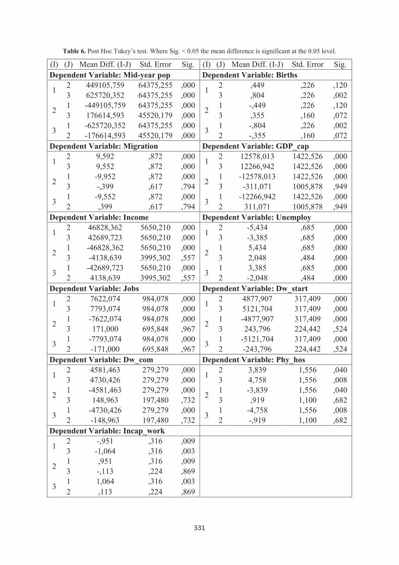
Most of the indicators, however, show significant differences among the various types of regions. It can be clearly seen already from the graphs in Fig. 2 that at least one region issignificantly different from others. Each box represents one type of a region. Only in case of the number of birth and physicians in hospitals, the differences are not visible on the first sight and must be tested (see Box, 1953 and Box, 1954-b). The results of the tests are displayed in Table 5. ANOVA revealed significant differences in all economic and labour market indicators. Also in most of the population and construction criteria, there are difference between PR, IN and PU regions. These are mid-year state of population, live births per 1 000 population, migration per 1 000 population, GDP per capita, income per capita, unemployment, job vacancies, dwellings started and completed, recalculated number of physicians in hospitals per 10 000 population and average incapacity for work. When these statistically significant differences among regions were found, Tukey’s Post hoc test was used to further analyze between what regions the differences are. The results of the calculations are presented in Table 6.

328

Fig. 1. Box and Whisker plots for indicators, where is not a statistically significant difference between the means

Contrary to expectation the test further revealed that in case of variable mid-year population

and unemployment, there are not statistically significant differences between two pairs of

live births per 1 000 population between PU and IN regions and between IN and PR. Surprisingly the PU and PR do not differ. In case of the migration increase/decrease per

1 000 population, GDP per capita, disposable income of households per capita, jobs

vacancies and dwelling started or completed, only difference were between IN and PR. Again, PU and PR were similar as same as PU and IN. There were statistically significant differences in the number of physicians in hospitals per 10 000 population between IN and PR

differences between PU and IN region. In any case could be found difference between PU and PR region. In average incapability for work, again, only IN and PR regions differ.

329

Table 5. ANOVA for indicators, where is a statistically significant difference between the means

Source Sum of Squares Df Mean Square F-Ratio P-ValueMid-year population

Between groups 5,30E+12 2 2,65E+12 47,35 0,0000Within groups 6,88E+12 123 5,59E+10Total (Corr.) 1,22E+13 125Live births per 1 000 population

Between groups 9,47716 2 4,738580 6,84 0,0015Within groups 85,1503 123 0,692279Total (Corr.) 94,6275 125Migration increase/decrease per 1 000 population

Between groups 1471,67 2 735,835 71,63 0,0000Within groups 1263,58 123 10,2730Total (Corr.) 2735,25 125Gross domestic product per capita

Between groups 1,85E+09 2 9,27E+08 43,62 0,0000Within groups 2,02E+09 95 2,12E+07Total (Corr.) 3,87E+09 97Disposable income of households per capita

Between groups 1,74E+10 2 8,71E+09 36,4 0,0000Within groups 1,60E+10 67 2,39E+08Total (Corr.) 3,35E+10 69Registered unemployment rate

Between groups 413,427 2 206,713 32,68 0,0000Within groups 778,123 123 6,32621Total (Corr.) 1191,55 125Job vacancies

Between groups 9,17E+08 2 4,59E+08 35,08 0,0000Within groups 1,61E+09 123 1,31E+07Total (Corr.) 2,53E+09 125Dwellings started

Between groups 3,87E+08 2 1,94E+08 142,37 0,0000Within groups 1,67E+08 123 1,36E+06Total (Corr.) 5,55E+08 125Dwellings completed

Between groups 3,35E+08 2 1,68E+08 159,1 0,0000Within groups 1,30E+08 123 1,05E+06Total (Corr.) 4,65E+08 125Physicians in out-patient care establishments per 1 000 population

Between groups 307,959 2 153,98 4,71 0,0107Within groups 4020,77 123 32,6892Total (Corr.) 4328,73 125Average incapacity for work

Between groups 16,0128 2 8,00642 5,92 0,0035Within groups 166,278 123 1,35185Total (Corr.) 182,291 125

330

Fig. 2. Box and Whisker plots for indicators, where is a statistically significant difference between the means

331

Table 6. Post Hoc Tukey’s test. Where Sig. < 0.05 the mean difference is significant at the 0.05 level.

(I) (J) Mean Diff. (I-J) Std. Error Sig. (I) (J) Mean Diff. (I-J) Std. Error Sig.Dependent Variable: Mid-year pop Dependent Variable: Births

12 449105,759 64375,255 ,000

12 ,449 ,226 ,120

3 625720,352 64375,255 ,000 3 ,804 ,226 ,002

21 -449105,759 64375,255 ,000

21 -,449 ,226 ,120

3 176614,593 45520,179 ,000 3 ,355 ,160 ,072

31 -625720,352 64375,255 ,000

31 -,804 ,226 ,002

2 -176614,593 45520,179 ,000 2 -,355 ,160 ,072Dependent Variable: Migration Dependent Variable: GDP_cap

12 9,592 ,872 ,000

12 12578,013 1422,526 ,000

3 9,552 ,872 ,000 3 12266,942 1422,526 ,000

21 -9,952 ,872 ,000

21 -12578,013 1422,526 ,000

3 -,399 ,617 ,794 3 -311,071 1005,878 ,949

31 -9,552 ,872 ,000

31 -12266,942 1422,526 ,000

2 ,399 ,617 ,794 2 311,071 1005,878 ,949Dependent Variable: Income Dependent Variable: Unemploy

12 46828,362 5650,210 ,000

12 -5,434 ,685 ,000

3 42689,723 5650,210 ,000 3 -3,385 ,685 ,000

21 -46828,362 5650,210 ,000

21 5,434 ,685 ,000

3 -4138,639 3995,302 ,557 3 2,048 ,484 ,000

31 -42689,723 5650,210 ,000

31 3,385 ,685 ,000

2 4138,639 3995,302 ,557 2 -2,048 ,484 ,000Dependent Variable: Jobs Dependent Variable: Dw_start

12 7622,074 984,078 ,000

12 4877,907 317,409 ,000

3 7793,074 984,078 ,000 3 5121,704 317,409 ,000

21 -7622,074 984,078 ,000

21 -4877,907 317,409 ,000

3 171,000 695,848 ,967 3 243,796 224,442 ,524

31 -7793,074 984,078 ,000

31 -5121,704 317,409 ,000

2 -171,000 695,848 ,967 2 -243,796 224,442 ,524Dependent Variable: Dw_com Dependent Variable: Phy_hos

12 4581,463 279,279 ,000

12 3,839 1,556 ,040

3 4730,426 279,279 ,000 3 4,758 1,556 ,008

21 -4581,463 279,279 ,000

21 -3,839 1,556 ,040

3 148,963 197,480 ,732 3 ,919 1,100 ,682

31 -4730,426 279,279 ,000

31 -4,758 1,556 ,008

2 -148,963 197,480 ,732 2 -,919 1,100 ,682Dependent Variable: Incap_work

12 -,951 ,316 ,0093 -1,064 ,316 ,003

21 ,951 ,316 ,0093 -,113 ,224 ,869

31 1,064 ,316 ,0032 ,113 ,224 ,869

332

4 Conclusion

The objective of this article was to assess how the rural areas differ from the urban areas in certain features important for rural development. Indicators from the area of demography, economics, labour market, construction, healthcare and social security were taken. The differences among values of particular indicator in predominantly rural (PR), intermediate (IN) and predominantly urban (PU) areas were tested using ANOVA method. In case of deaths per 1 000 population, average living floor area per completed dwelling, physicians in

out-patient care establishments per 1 000 population, beds in hospitals per 1 000 population

and average old-age pension, there were no statistically significant differences found.

On the other hand, based on the results of Tuckey’s test, the most dissimilarities were found between IN and PR regions. They differ in migration increase/decrease per 1 000 population,GDP per capita, disposable income of households per capita, jobs vacancies and dwelling

started or completed. This clearly shows that PU and PR regions are not always that dissimilar as stated. Our findings speak for the urban-rural continuum theory rather than for the rural definition based on the distinction between rural and urban. Many researchesconsider PR areas unfavorable, but our results show that it is not always the case. In average they do not differ in the majority of indicators used to measure the development state of the region. PR regions are disadvantaged only in both economic indicators.

There are several possibilities for future research. In the first place it would be advantageous to obtain a longer time series of the indicators. The analysis, which was introduced in this paper, then could be performed separately, i.e. after certain time periods. Another possibility is to use that longer time series and make the predictions using one of the methodological approaches for modeling time series (see e.g. Box and Jenkins, 1968, or Box, Jenkins and MacGregor, 1974 or Ray, 1982). With the predicted values then would be also performed ANOVA and with the time delay could be compared how the estimated values differ from the actual, that will emerge from the empirical data.

Acknowledgements

The paper is supported by the internal grant: “Využití rozvoj venkova” No. 20121054:11110/1312/3112 of the Internal Grant Agency of the Faculty of Economics and Management of the Czech University of Life Sciences in Prague.

References

Berkel, D. B., Verburg, P. H. (2011) Sensitising rural policy: Assessing spatial variation in

rural development options for Europe. Land Use Policy. Vol. 28, pp. 447–459.

Binek, J. et al. (2009). Synergie ve venkovském prostoru.Brno: GaREP, spol. s r.o., p. 96. ISBN 978-80-904308-0-8.

Binek J., Svobodová H. (2009). Rural Development and Regional Development: Common Agricultural Policy and Regional Policy on one field. Czech Regional Studies, Vol. 3, Issue 1, pp. 12-18.

Box, G.E.P. (1953). Non-Normality and Tests on Variances. Biometrika (Biometrika Trust)

40 (3/4): 318–335.

333

Box, G.E.P. (1954-a). Some Theorems on Quadratic Forms Applied in the Study of Analysis of Variance Problems, II. Effects of Inequality of Variance and of Correlation Between Errors in the Two-Way Classification. The Annals of Mathematical Statistics 25 (3): 484.

Box, G.E.P. (1954-b). Some Theorems on Quadratic Forms Applied in the Study of Analysis of Variance Problems, I. Effect of Inequality of Variance in the One-Way Classification. The

Annals of Mathematical Statistics 25 (2): 290.

Box, G.E.P. and Jenkins G.M. (1968). Some Recent Advances in Forecasting and Control, Part I. Journal of the Royal Statistical Society. Series C (Applied Statistics). Vol. 17, No. 2, 1968, p. 91-109.

Box, G.E.P., Jenkins G.M. and MacGregor J.F. (1974). Some Recent Advances in Forecasting and Control, Part II. Journal of the Royal Statistical Society. Series C (Applied Statistics).Vol. 23, No. 2, 1974, p. 158-179.

Cohen, J. (1988). Statistical power analysis for the behavior sciences (2nd ed.). Routledge ISBN 978-0-8058-0283-2.

Eurostat (2012). Urban-rural typology. Last modified on 15 May 2013, at 15:56. Available from <http://epp.eurostat.ec.europa.eu/statistics_explained/index.php/Urban-rural_typology>

Friedland, W. H. (2002). Agriculture and Rurality: Beginning the “Final Separation”?, Rural

Sociology, vol. 67, no. 3, pp. 350–371.

Halfacree, K. H. (1993). Locality and Social Representation: Space, Discourse and Alternative Definitions of the Rural, Journal of Rural Studies, vol. 9, no. 1, pp. 23-37.

Chevalier, P. (2008). Diversification and transformation of the economic base in Czech rural areas. Revue d'études comparatives Est-Ouest, Vol. 39, Issue 4, (December 2008), p. 143-+.

Jánský, J. (2012). Metodické postupy k hodnocení disparit v . In: Sborník

-ROM].s. 105-119. ISBN 978-80-7375-652-9.

Linton, L.R., Harder, L.D. (2007). Biology 315 – Quantitative Biology Lecture Notes.University of Calgary, Calgary, AB

Margarian, A. (2013). A Constructive Critique of the Endogenous Development Approach in the European Support of Rural Areas, Growth and Change, vol. 44, no. 1, pp. 1–29.

Countryside in the Czech Republic – determination,criteria, borders,Agricultural Economics, vol. 53, no. 6, pp. 247–255.

McGill, R., Tukey, John, W., Larsen, Wayne, A. (1978). Variations of Box Plots. The

American Statistician 32 (1): 12–16.

Ministry of Rural Development (MRD) (2012). Strategy of Regional Development of CR for period 2014–2020. Available from <http://www.mmr.cz/getmedia/5acbe736-6893-4ff6-b548-c3d5b57dbc83/SRR-(2012-12-11).pdf>.

Ministry of Agriculture (2013). Rural Development Programme of the Czech Republic.

Mosteller, F., Tukey, John, W. (1977). Data analysis and regression. A second course in

statistics. Addison-Wesley Series in Behavioral Science: Quantitative Methods, Reading, Mass.: Addison-Wesley, 1977.

334

-27 for SpatialAnalysis: Rural Labour Market Approach. Integrated and Sustainable Rural Development.

Rural Development, vol. 2009, pp. 127-134.

Ray W.D. (1982). ARIMA Forecasting Models in Inventory Control. The Journal of the

Operational Research Society, vol. 33, No. 6, Jun., 1982, p. 567-574.

Surchev, P. (2010). Rural Areas – Problems and Opportunities for Development. Trakia

Journal of Science, vol. 8, no. 3, pp. 234-239.Tisenkopfs, T (1999). Rurality as a created field: Towards an integrated rural development in Latvia? Sociologia Ruralis, vol. 39, no. 3, pp. 411-430.

EU Rural Development Policy: the Case of the Czech Republic. Rural

Development In Global Changes, vol. 5, no. 1, pp. 254-260.

Vobecká, J. (2009). Czech Rural Development Policies for Human Resources after 2004: A Story of Muddled Definitions Preventing Strategic Visions?. Central European Journal of

Public Policy, vol. 2009, no. 1, pp. 44- 65.

Westhoek, H.J., van den Berg, M., Bakkes, J.A. (2006). Scenario Development to Explore the Future of Europe’s Rural Areas, Agriculture, Ecosystems and Environment, vol. 114, no. 29, pp. 7-20.