running head: spatial analysis of changes in the unemployment rate · · 2015-01-22explaining...

Research in Business and Economics Journal

Spatial analysis of change, page 1

Spatial analysis of changes in the unemployment rate: A county-

level analysis of the New England states

Zachary A. Smith

Saint Leo University

ABSTRACT

This research project examines the spatial dependence of unemployment rates during a

period of economic uncertainty occurring at a tract level of analysis in the New England States.

The spatial components used to describe spatial dependence in unemployment rates are physical,

ethnic, and occupational distances. The researcher identified statistically significant levels of

spatial dependence using each of the distance metrics (α = .10); however, the economic and

statistical significance of the physical distance metric dominates the other two spatial variables

(p value of less than .001 and an R2 value of .3367). Furthermore, in this project, the researcher

was able to improve the coefficient of determination for the final model used to estimate changes

in unemployment rates from .201 to .694 by adding spatially dependent variables to the

traditional independent socioeconomic variables in a multivariate regression analysis.

Keywords: Unemployment Rates, Spatial Dependence, Physical Distance, Ethnic Distance,

Occupational Distance

Copyright statement: Authors retain the copyright to the manuscripts published in AABRI

journals. Please see the AABRI Copyright Policy at http://www.aabri.com/copyright.html.

http://www.aabri.com/copyright.html



INTRODUCTION

Following the research of Conely and Topa (2002), this project attempts to estimate

social interaction effects and use the estimates of these parameters to understand how social

interaction effects influenced changes in the unemployment rate as the U.S. Economy entered

into a recessionary climate in 2008. To accomplish this task the researcher used three different

socioeconomic distances (i.e. geographic, ethnic, and occupational) as well as traditional

economic variables believed to have some explanatory power over potential changes in county-

level unemployment rates. This paper finds that these socioeconomic distances have significant

explanatory power over the changes in the unemployment rates for the 67 counties included in

this study.

To explore the social characteristics that might be associated with changes in the

unemployment rate during a period of economic uncertainty, the researcher had to identify both a

time prior to the decline in the general economy (i.e. a peak in the business cycle) and a low

point (i.e. a trough in the business cycle). To accomplish this, the researcher reviewed the

changes in the Gross Domestic Product (GDP) leading up to the most recent recession, which

occurred in the last quarter of 2008. From 2006 to 2008, the unemployment rate and the

percentage change in the GDP of the U.S. had been negatively correlated and seemed to display

substantial dependence—see Figure 1.

It has been established that the unemployment rate is a lagging indicator of economic

activity; therefore, it will presumably take a number of periods for changes in GDP to affect the

labor market. The consumer has a substantial influence over this relationship, as consumers’

demand less producers will respond by supplying less. Producers will supply fewer goods and

services to deal with a lower demand, thus, will require less labor. Hence, the researcher should

be able to describe changes in the unemployment rate using current and lagged GDP data.

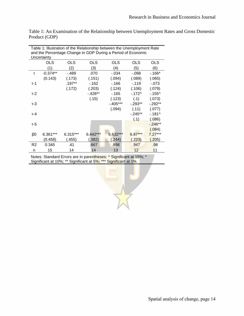
Table 1 shows the relationship between the Unemployment Rate and GDP data using

various lags of the change in U.S. GDP from 2006 to 2008. It is evident, at least using this time

horizon, that the relationship between lagged GDP and the unemployment rate is significant.

This model generates an R2 of .98 at lag five. The researcher carried this exercise out to

determine when the study should start and when the study should end—the researcher has

determined that the study should be run from the first quarter of 2006 to the fourth quarter of

2008 to capture the change in unemployment rate from the peak of the cycle to the trough.

LITERATURE REVIEW

Akerlof, G. (1980) stated, in an analysis of social customs and their influence on

unemployment, that “a custom, once established, will persist, provided that the disobedience of

the custom results in sufficient loss of reputation, and provided that the cost of disobedience is

sufficiently high” (p. 751). Moreover, Akerlof, G. (1980), concludes that “a custom, that is fairly

costless to follow will, once established, continue to be followed because persons lose direct

utility by disobeying the underlying social code and also because, according to the model,

disobedience of social customs will result in loss of reputation” (p. 772). The general idea

presented in Akerlof, G. (1980), has a profound influence on how researchers can think about

social interaction effects and their influence on the actions of policy makers, individual agents,

and in the aggregate at a county level of analysis. Customs permeate our culture and whether

researchers are analyzing individual or county level interactions, the customs that have been



established regionally or based upon an individual’s ethnic or occupational affiliations cause a

clustering of like individuals amongst various socio-economic groupings.

Customs, and an individual’s likeliness to obey these customs, influence their behavior

and therefore, their choices by influencing the perceived utility of a perspective outcome based

upon potential negative externalities that arise from disobeying an established custom. Akerlof,

G. (1997) explains that social externalities arise from social interactions and posits that an

agent’s choice to maximize their expected outcome may be influenced by their social affiliations

with other agents in a particular locality; furthermore, that “group interactions are an important

influence on individual decisions; [therefore,] the analysis of social programs must include an

evaluation of an intervention’s impact on group interactions and not just the direct affects of the

program” (Akerlof, G., 1997, p. 1023). Ioannides and Topa (2010), likened this concept of social

interactions and the implicit effect that social interactions or groupings have on behavior by

explaining that “social interdependencies emerge naturally if individuals share a common

resource or social space in a way that is not paid for but still generates constraints on individual

action” (p. 244). Therefore, our social position, whether it is geographic or socio-economic, has a

profound effect on an individual’s perceived economic outcomes.

Conley and Topa (2002) use this general argument to analyze whether the social

economic distance between two agents influences their ability to obtain employment. The

authors accomplish this by constructing physical, ethnic, and occupational distances between the

various tracts in Chicago and examine whether the distances between two tracts have

explanatory power over their respective unemployment levels. However, Conley and Topa

(2002) question whether the Census Tract Level is the appropriate scale of analysis to use to

evaluate social interaction effects; specifically, whether “most actions take place at lower levels

of agglomeration” (p. 25). Akerlof, G. (1997) echoed this question and stated “that the

community is endogenously defined in terms of peoples’ sense of location. What may appear as

a community to an outside reformer…may be too large a unit in which to encompass the social

interactions involved in social exchange” (p. 1023). This research project questions these two

statements and examines whether researchers might be able to examine the effects of these social

interactions using a county level of analysis during a period of economic uncertainty.

As Conley and Topa (2002) discussed, developing “a better understanding of the likely

components of socio-economic distance will greatly facilitate the estimation of social interaction

effects” (p. 304). This paper builds on the research conducted by Conley and Topa (2002),

focusing specifically on applying the socio-economic distances that they used to estimate the

social interactions effects at a tract-level of analysis in the city of Chicago and applies them at a

county-level analysis in the New England States. Based upon a strength of position as well as a

basic argument for and against the maintaining strong social ties Ioannides and Loury (2004)

illustrated how these social interactions could cause a sorting of individuals into various

networks. Applying the sentiment of Conely et al. (2002) to Ioannides et al. (2004), the

researcher can reasonably test for evidence of clustering behavior among people with similar

preferences and tastes at a county level of analysis.

According to Conley and Topa (2002), employees find employment approximately 50%

of the time through social networks (p. 304). Ioannides and Loury (2004) also found that the

following four elements are critical factors that should be explored to understand how job

networks influence labor market outcomes: (a) employer, (b) relational, (c) contact, and (d)

worker heterogeneity (p. 1061—see Table 2 for a categorization of the variables used in this

study). This research project’s basic model has components of three of the four critical factors



that Ioannides and Loury (2004) have indicated effect labor-market outcomes (i.e. relational,

contact, and worker heterogeneity)—the researcher did not add employer-related factors in this

analysis. Ioannides et al. (2004) indicated that “contact and relational heterogeneity respectively

denote variations in the resource endowments of one’s associates and the social relationships that

allow individuals to claim access to resources possessed by their associates” (p. 1061); whereas,

worker heterogeneity refers to differences in worker productivity or other characteristics

(Ioannides et al., p. 1061). Both types if heterogeneity seems to possess substantial explanatory

power over socio-economic interactions and outcomes.

This studies main goal is to determine whether researchers could use spatially dependent

variables to improve a model’s ability to forecast changes in the unemployment rate of a

particular county as the U.S. Economy’s business cycle went from peak to trough from the first

quarter of 2006 to the fourth quarter of 2008. According to Topa (2001), agents’ choices and

payoffs are affected by other agents’ actions, not just indirectly through markets, but also directly

through imitation, learning, social pressure, information sharing, or other non-market

externalities…It is also assumed that agent[s] interact locally, with a set of neighbors defined by

an economic or social distance” (p. 261). The researcher believes that this analysis will find that

as the geographic, ethnic, and occupational distances between two agents increase, their actions

will become increasingly dissimilar; moreover, that neighboring county’s unemployment rates

will influence a particular county’s unemployment rate. The researcher will use the concept of

spatial dependence, and tests constructed to identify spatial dependence, to identify if and where

social interaction effects occur and the extent of these interaction effects.

DATA

For this project, the researcher collected data from a variety of sources. For the traditional

economic variables, the researcher used the U.S. Census Bureau’s American FactFinder Fact

Sheet (URL: http://factfinder.census.gov) to obtain 3-year estimates, from 2006-2008, for the

following variables: (a) The percentage of the population 25 years and over, (b) The percentage

of the population that is a high school graduate or higher, (c) The percentage of the population

that has a Bachelor’s Degree or higher, (d) Per capita income, (e) The percent of families below

poverty level, and (f) The percent of individuals below the poverty level. The researcher used

information from U.S. Census Bureau’s American FactFinder website, listed above, to obtain

information pertaining to the ethnic composition of a particular county. Estimates of the counties

occupational breakdown by NAICS code was taken from the U.S. Census Bureau 2002

economic census (URL: http://www.census.gov/econ/census02/data/nc/NC001.HTM).

Unemployment data was found on the Bureau of Labor Statistic’s website: ww.bls.gov. Finally,

the researcher obtained the latitude and longitudinal coordinates to determine the physical

distance between two counties.

METHODOLOGY

This study expands the research conducted by to Conley and Topa (2002), in which they

found significant levels of physical, ethnic, and occupational dependence occurring in their

analysis of unemployment rates at a tract level of analysis in the City of Chicago. The researcher

builds on their study by examining the following research questions using a county level of

analysis.

http://factfinder.census.gov/

http://www.census.gov/econ/census02/data/nc/NC001.HTM



Research Question 1: Is there evidence of spatial dependence in the spatial lags of physical,

ethnic, and occupational distances?

Research Question 2: How well do the spatial lags of physical, ethnic, and occupational

distances explain the changes in unemployment rates during a period of economic uncertainty?

Research Question 3: How well do variables traditionally used explain unemployment rates

predict changes in unemployment rates during a period of economic uncertainty?

Research Question 4: Can researchers use a mixture of traditional variables and spatially lagged

variables to improve the predictive power of a regression analysis to predict changes in

unemployment rates during a period of economic uncertainty?

The following sections provide an answer to these research questions.

This paper’s attempt to explain what factors may have caused changes in the

unemployment rate during the recent economic downturn relied on both spatially dependent and

traditional independent variables. The traditional independent variables are: (a) The log of the

average per capita income, (b) The percent of families living below the poverty rate, (c) The

percent of individuals living below the poverty rate, (d) The percent of individuals that have a

high school education or higher, (e) The percent of individuals that have greater than a

bachelor’s degree, and (f) The percent of the population that are 16 years or older. The spatially

dependent variables are as follows, the spatial lag of the difference in the unemployment rate

during the economic downturn with respect to: (a) Physical Distance, (b) Ethnic Distance, and

(c) Occupational Distance. The complete model is presented below:

�̂�𝑖 = 𝛼𝑖 + 𝜌𝑊1𝑦𝑖 + 𝜑𝑊2𝑦𝑖 + 𝛿𝑊3𝑦𝑖 + 𝛽1𝑥1,𝑖 + 𝛽2𝑥2,𝑖 + 𝛽3𝑥3,𝑖 + 𝛽4𝑥4,𝑖 + 𝛽5𝑥5,𝑖 + 𝛽6𝑥6,𝑖 + 휀

�̂�𝑖: Estimated Difference in Unemployment Rates

𝛼𝑖: Intercept term

𝜌𝑊1𝑦𝑖: Spatial Lag of the Difference in the Unemployment Rate in respect to ‘Travel

Distance (Auto)’

𝜑𝑊2𝑦𝑖: Spatial Lag of the Difference in the Unemployment Rate in respect to ‘Ethnic

Distance’

𝛿𝑊3𝑦𝑖: Spatial Lag of the Difference in the Unemployment Rate in respect to

‘Occupational Distance’

𝛽1: The beta coefficient for the log of the average Per Capita Income

𝛽2: The beta coefficient for the % of families living below the poverty rate

𝛽3: The beta coefficient for the % of individuals living below the poverty rate

𝛽4: The beta coefficient for the % of individuals that have a high school education or

higher

𝛽5: The beta coefficient for the % of individuals that have greater than a bachelor’s

degree

𝛽6: The beta coefficient for the % of the population that are 16 years or older

휀: Error Term



Spatial Components

This research project used three different spatial components. The first, is based upon

physical distance and it takes two forms: (a) the neighbor effects or ‘boundary sharing’ and (b)

travel distance or how far, in terms of geographic miles, one county resides in comparison to

another (typically, the researchers used the mid-points of the counties to run this calculation).

The second neighborhood effect explored in this study is ethnic distance. When researchers

examine the ethnic distance between two counties, they are evaluating how similar counties are

to one another with respect to their population’s ethnic breakdown and from this an ethnic

distance is calculated. The final distance metric that was calculated in this study was the

occupational distance between counties. The occupational component is similar to the ethnic

component, in that it compares the occupational breakdown found in one country against another

and estimates their distance in terms of ‘likeness’ or ‘similarity’. The following sections provide

an explanation of how each of these metrics was calculated.

Physical Distance

Physical distance is the easiest distance metric to explain. Everyone has had experiences

traveling and whether measured in time or distance traveled, there is a cost associated with their

travel. The distance traveled can be thought of as a cost associated with the activity that

provoked them to travel. This study takes this concept and applies it to county-level interactions

by first stating that if a county shares a boundary with an adjoining county (first spatial lag of

geographic distance), that county is more likely to interact with the adjoining county than it is

likely to interact with counties that do not share a boundary. Next, this project analyses how

quickly the neighbor’s influence on the county of interest deteriorates as the distance between the

two counties increases. By using this strategy to analyze the neighborhood effects, researchers

can show how quickly the spatial dependence between two counties deteriorates and at what

point the dependence between the two counties becomes insignificant.

Ethnic Distance

It has been shown that people with similar ethnic backgrounds are more likely to

associate with each other (see Ioannides & Loury, 2004, p. 166), when compared against people

with different ethnic backgrounds. Furthermore, if the community that an individual agent

resides has a greater proportion of agents that possess a similar ethnic background, those agents

are likely to have a greater chance of uncovering employment opportunities through networking

in those groups than they would otherwise (Conley & Topa, 2000, p. 10 and Ioannides et al.,

2004). This research project posits that counties that have similar ethnic structures will have

similar unemployment rates, all other things equal; so, theoretically, spatial dependence is likely

to exist between counties that have similar ethnic compositions. A modified formula taken from

Conley and Topa (2002) that the researcher used to calculate ethnic distance is as follows:

𝑒𝑑𝑖,𝑗 = ∑ √(𝑒𝑖,𝑘 − 𝑒𝑗,𝑘)27𝑘=1 Equation 2

𝑒𝑑𝑖,𝑗: Ethnic distance between agent i and j

ek: % Ethnicity of agent i

ej % Ethnicity of agent j through k



After the researcher calculated the ethnic distance between each of the counties included in the

study, the distances between counties were used to construct the weight matrices. The ethnic

distance variable indicates how far each counties ethnic structure was from each of the other

counties in the sample. Using this structure to construct the spatial lag ethnic distance, the most

weight would be given to the county that is least like the target county, in terms of ethnic

composition; therefore, the Moran’s I, the test for spatial dependence, should turn out to be

negative if there is spatial dependence.


According to Conley and Topa (2002), individuals with similar occupational

backgrounds are “more likely to convey useful information about job openings, or generate

referrals” to the currently unemployed (p. 310). This research project projects this general

statement on a county of individuals and makes inferences about the benefits of these kinds of

relationships using the following calculation (Conley et al., 2002, p. 311):

ODi,j = ∑ √(oi,k − oj,k)212

k=1 Equation 3

odi,j: Occupational distance between agent i and j

oi : Number of people employed in occupation k

oj Number of people employed in occupation i at location j

The occupational distance variables used in this study share the same properties as the ethnic

distance variables. That is, if the researcher was to use the raw distance, the county with the

greatest distance from the county of interest would generate the greatest weight in the weight

matrices; therefore, the coefficients are expected to be negative.

Spatial Lag Model

To determine whether a specific variable is spatially dependent, researchers need to

calculate the ‘spatial lag of the variable of interest’. In all three of the spatial dependence

calculations used in this project, the researcher will have to determine a way to define a

neighborhood. Typically, the distances between two counties would be used to construct a

connectivity matrix (C), which is an n x n matrix, where nth

is each county contained in the

sample (the exception to this approach is using the raw distance score to construct the weight

matrix using travel distance, which can be seen in Tables 4b and 4c). If county i and county j are

considered neighbors, within the matrix, the row-column match between counties i and j will

take on a value of one (or in the case of ethic and occupational distance a distance score will be

calculated base upon the aforementioned distance metrics); otherwise, this row-column match

will take on a value of zero.

Next, the researcher took this connectivity matrix (C) and transformed it to a row-

normalized connectivity weight matrix (W) where each row sums up to one by dividing each ci

of the binary connectivity matrix C by the total number of links ∑ci∙ (Ward, M. and Gleditsch,

K., 2008, pg. 18). Furthermore, Ward et al. (2008) explained that researchers can use the scalar

yis = ci∙ ∗ y, the spatial lag of y on itself, using the W to describe the connectedness of each



neighboring observation of unit i to estimate the spatial dependence embedded in the sample (p.

18); therefore, the spatial lag of y is the average of all of the neighbors of y in lag i. This study

applies the spatially lagged model to explain the dependence between the county of interest and

its spatial lag. When researchers use a spatially lagged model, they are assuming, according to

Ward and Gleditsch (2008) that “they believe that the values of y in one unit i are directly

influenced by the values of y found in i’s ‘neighbors’” (p. 35). The reader can compare this

model with spatial error model, in which, according to Ward et al. (2008), researchers treat the

spatial correlation as a nuisance that should be eliminated—this nuisance will lead to estimation

problems (p. 65). This project assumes that there is information embedded in ‘neighborhood’

that will have significant explanatory power over what happens in the county of interest. This

paper uses the Moran I statistic to proxy for spatial dependence; formally, this metric can be

calculated using the following formula (Ward and Gleditsch, 2008, p. 23):

𝐼 =𝑛∑ ∑ 𝑤𝑖𝑗(𝑦𝑖−�̅�)(𝑦𝑗−�̅�)𝑗≠𝑖𝑖

(∑ ∑ 𝑤𝑖𝑗)𝑗≠𝑖𝑖 Equation 4

RESULTS

This section evaluates: (a) Moran’s tests for spatial dependence using different lags and

weighting structures for each of the distance metrics used in this study, (b) Models that estimate

the change in unemployment rates using traditional and spatially dependent variables, and (c) A

final model using traditional and spatial components to estimate the changes in unemployment

rates. The section will start by reporting the results of the spatial dependence between the

percentage change in the unemployment rates and the physical, ethnic, and occupational

distances between counties. Next, the researcher presents the results of an OLS regression using

the traditional independent variables outlined in previous sections. The researcher then estimated

the spatial dependence found in each of the spatially dependent variables indentified in this

study. Finally, the variables are combined and an OLS regression is run to determine what mix of

spatially dependent and traditional variables generated the best estimation of the changes in

unemployment rates experienced in a period of economic uncertainty.

Physical Distance

For this portion of the analysis, the researcher used three different weighting schemes;

Table 4 presents the results. It is evident that Weighting Scheme 2, produces the most significant

results using the first neighbor strategy (i.e. lag 1), but a thorough examination of both

Weighting Schemes 1 and 2, would portray what Conley and Topa (2002) conveyed in their

paper, which is that “spatial correlation decays roughly monotonically with distance” (p. 325).

The researcher presents evidence of this by graphing the Moran’s I on the upper distance limit of

each respective lag, as seen in Figure 2. In Figure 2, the spatial dependence between the change

in the unemployment rates and physical distance goes from a very strong relationship when

neighbors reside within 20 miles of the target county, diminishes quite rapidly as they move from

20 to 60 miles, and then deteriorates and becomes insignificant from 60 to 80 miles.

The researcher chose to use the 2nd weighting scheme, bordering county, because the

spatial dependence found using this method was the most significant; however, the strength of

the spatial dependence was very similar to specifying ‘a neighborhood’ as counties within 20

miles of the county of interest. To carry out this analysis the researcher constructed a



connectivity matrix (C) using the criteria set for weighting scheme 2, lag 1 (i.e. the counties must

share a border) in Table 4b. The spatial dependence between the percentage change in the

unemployment rates and geographic distance (identified by the Moran I test statistic) is .5803

and significant using an α of less than .001. As the researcher altered the connectivity matrix,

moved to the second lag (i.e. separated the counties by another county and required both counties

share a border with the county that separates them), the spatial dependence between the

percentage change in the unemployment rates and geographic distance deteriorates to .1930 and

is insignificant using an alpha of less than .10. Since the spatial dependence is no longer

significant at Lag 2, the researcher will create the spatial lag used in the OLS regression analysis,

by constructing the connectivity matrix using the first lag of the second weighting scheme.

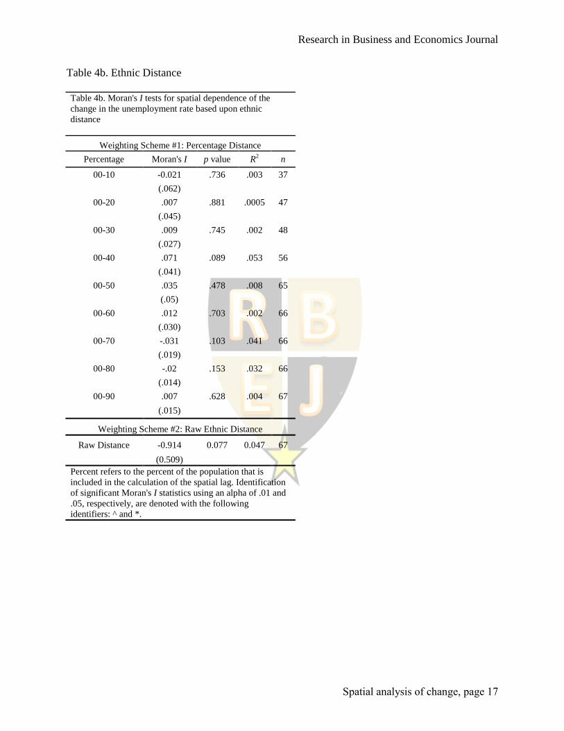
Ethnic Distance

To determine whether changes in unemployment rates exhibited spatial dependence in

terms of ethnic distance, the researcher constructed two different weighting schemes and

displayed the results of these test for spatial dependence in Table 4b. The researcher based the

first weighting scheme, percentage cohorts, upon the first physical distance-weighting scheme in

Table 4a. If the distance between two counties was smaller than 90% of the distances between

the other counties in the sample, then this particular relationship would be examined in the 00 –

10 percent lag (if smaller than 80 percent of the distances in the population, the relationship

would be evaluated in the 00 - 20 lag). The researcher initially assumed that if a county’s ethnic

composition is similar to another, changes in their unemployment rates might also be similar—

and, spatial dependence would be evident in the sample. This did not happen; weighting structure

1 produced no economically or statistically significant results, in terms of spatial dependence.

Since the percentage distance weighting used in Weighing Scheme 1 failed to produce

any significant results the researcher ran a Moran test using the raw ethnic distances calculated

by Equation 2. The results were not significant using an α of .05, but there is a weak statistical

relationship between the change of unemployment rates and ethnic distances that is statistically

significant using an α of .10. Since this, the raw ethnic distance weighting procedure, is relatively

easy to describe and recreate the researcher has chosen to use this weighting procedure to run the

regression analyses.


Initially, for the analysis of occupational distance, the researcher started out using a

weighting structure similar to the one used to estimate the spatial dependence between the

change in unemployment rates and physical distance (i.e. Table 4b); again, the researcher is

attempting to determine if spatial dependence decreases monotonically as the occupational

distance between counties increases. This analysis found no evidence of this. Conley and Topa

(2002) stated that, both distance metrics (i.e. ethnic and occupational) had strong and negative

spatial dependence when the distance grew substantially large between the two counties;

therefore, if this project is not able to identify spatial dependence using small occupational

distances, it may be useful to try to use greater occupational distances. The results of the Moran

tests for these lags are presented in Table 4c at distances of greater than 30, greater than 40, and

greater than 50 percent. The results do not seem to support the findings Conley et al. (2002) that

strong and negative spatial dependence occurs when the distance grows substantially large



between the two counties, because there was an insignificant, but negative (which supports

Conley et al.) relationship at distances that are greater than the bottom 80% of the population.

Since the relationship between occupational distance and changes in the unemployment rates

seems to be complex, the researcher chose the simplest weighting scheme to describe the spatial

dependence using this metric, Weighting Scheme 1 – Raw Distance. Using this weighting

scheme the researcher found that spatial dependence is statistically significant using an α of .10.

Using Spatial Variables to Predict Changes in the Unemployment Rate

After choosing weighting structures that coincide with evidence of spatial dependence

presented in the previous sections, the researcher was interested in examining how useful and

significant each of the spatial lags were in explaining changes in the unemployment rates. Table

5a presents the results of this stage of the analysis. All of the spatial lags based upon different

distances (i.e. physical, ethnic, and occupational) generated statistically significant results using

an α of .10, but it is obvious that the explanatory power embedded in the spatial lag, using

physical distance as the distance metric, far exceeds that of the other distances. As the researcher

added the two other spatial lags (i.e. based upon ethnic and occupational distance) to the physical

distance variable and attempted to explain changes in the unemployment rates, the R2 value

increases from .337 to .345. It seems obvious and is verified by conducting an F test (F statistic -

.4089) that the addition of these two spatially lagged variables offers very little additional

explanatory power that is not already included in the spatial lag of the physical distance.

Using Traditional Variables to Explain Changes in Unemployment Rates

In this section, the researcher determined to what extent changes in the traditional

independent variables explained changes in unemployment rates. The traditional variables used

in this study were: (a) The log of the average per capita income, (b) The percent of families

living below the poverty rate, (c) The percent of individuals living below the poverty rate, (d)

The percent of individuals that have a high school education or higher, (e) The percent of

individuals that have greater than a bachelor’s degree, and (f) The percent of the population that

are 16 years or older. In this round of the analysis, five counties were dropped from the study,

because the researcher could not obtain the data necessary to run a regression analysis including

all of the independent variables; the counties dropped from the analysis were: (a) Essex, (b)

Grand Isle, (c) Piscataquis, (d) Nantucket, and (e) Dukes.

The results of the regression analysis using traditional explanatory variables are presented

in Table 5b; the results were statistically significant using an α of less than .05. The traditional

dependent variables that displayed statistically significant explanatory power over changes in the

unemployment rates during a period of economic uncertainty were: (a) Per Capita Income, (b)

Family-Level Poverty, and (c) Education—obtaining a high school diploma or greater. The

results seem to coincide with some more general assumptions about employability: Typically,

people with (a) higher per capita incomes, (b) whose family lives above the poverty line, and (c)

have a greater than a high school education are more likely to have marketable skills when

compared against those who do not.



Regression Analysis

This section will present the final model and explain the relationship between the

percentage change in unemployment and the explanatory variables. This process will be

completed in five steps: (a) Construct an OLS regression analysis using only the physical lag of

the change in unemployment rates, (b) Include the remaining spatial components, (c) Use the

spatial lag of the change in unemployment rates based on physical distance and include the

traditional independent variables, (d) Add the remaining spatial lags to the preceding regression,

and (e) Omit the outliers from previous regression—see Table 5c for the regression results.

Again, it is necessary to state that five counties used to estimate the spatial dependence were not

included in the latter stage of the analysis because the data need to estimate the parameters for

the traditional independent variables were unavailable, these counties were: (a) Essex, (b) Grand

Isle, (c) Piscataquis, (d) Nantucket, and (e) Dukes.

Table 5c provides the results of the regression analyses and summarizes the general

findings. In Model 1, the researcher relied solely on the explanatory power of the spatial lag of

physical distance to explain changes in the unemployment rates. Again, the spatial lag of

unemployment rates base upon physical distance has substantial explanatory power over the

changes in unemployment rates experienced using a county level of analysis from 2006 to 2008.

The second iteration of this model, the addition of our spatial lags of ethnic and occupational

distance to the physical distance metric, improved the model’s explanatory marginally, but it

seems that the spatial lag of physical distance dominates the other two spatial components. In

Model 3, the researcher included only the spatial lag of physical distance and the traditional

explanatory variables to attempt to explain the changes in unemployment rates during this

period, again the results improve marginally. Finally, in Models 4 and 5, the researcher added

both the traditional and spatially lagged components to this analysis and omitted the outliers in

the spatially lagged ethnicity variables and, again, marginally improved the models predictive

power.

CONCLUSION

This paper’s main goal was to expand the research conducted by Conley and Topa (2002)

to determine if the researcher could find evidence of spatial dependence in terms of physical,

ethnic, and occupational distances using a county level of analysis. By expanding the unit of

measurement from a tract level to a county level, this project questions whether social interaction

effects are restricted to lower levels of agglomeration (Conley & Topa, 2002, p. 25) than a tract

level of analysis and whether researchers can use a county level of analysis to analyze aggregate

social interactions involved in social exchanges (Akerlof, 1997, p. 1023). In contrast to what

Conley and Topa (2002) found in their analysis of spatial dependence at a tract level of analysis,

in which the researchers found that the social interaction effects attached to physical,

occupational, and ethnic distance decreased monotonically with distance, the researcher finds

that the social interaction effects attached to physical distance decreases monotonically as

distance increases—this is not the case when the researcher evaluated the remaining social

interaction effects. The social interaction effects or spatial dependence found using the ethnic

and occupational distances, first, does not decrease as distances increase and, second, the

coefficients attached to the spatial dependence are negative and statistically significant. This

finding has interesting implications, to explain this phenomenon; the researcher needs to alter the



way researchers describe county level interactions in terms of ethnic and occupational distances

using a county level of analysis.

The spatial lags of ethnic and occupational distances illustrate an interesting structural

relationship that is occurring between these counties and is somewhat intuitive. As the

occupational and ethnic disparities between counties increase, the explanatory power of these

two metrics increases. The interpretation of this finding is that if a county is somewhat similar to

another county, in terms of ethnic and occupational structure, these two metrics have little

explanatory power over the directional changes in unemployment rates. However, as the counties

become increasingly dissimilar, in terms of occupational and ethnic make-up, the strength of

these metrics explanatory powers grows and trends toward generating statistically significant

spatial dependence between the two counties of interest. The dissimilarity between two counties

seems to have a statistically significant influence on changes in their unemployment rates.

Conley and Topa (2002) also found, in their analysis of social interactions at a tract level

of analysis is Chicago, that the Ethnic and Occupational Distances dominated the Physical

Distance metric in terms of spatial dependence. This study finds that the information embedded

in the physical distance metric dominates the other two proxies for social interaction effects;

moreover, after conducting a f test, the researcher determined that the Ethnic and Occupational

Distances did not contribute enough predictive power to be included in a model that uses only

spatially dependent variables to explain the changes in unemployment rates during a period of

economic uncertainty. Therefore, the information embedded in the Physical Distance metric

seems to dominate the social interaction effects inherent in the Ethnic and Occupational

Distances.

The final model illustrates how pervasive the effects of spatial lags, especially when

examining physical distance, are in terms of describing changes in our dependent variable (i.e.

changes in unemployment rates during a period of economic uncertainty). In this analysis,

relying solely on traditional independent variables to explain the changes in unemployment rates,

the researcher was able to generate a model that was statistically significant; however, the model

lacked economic significance. By including the spatial lag of physical distance with the

traditional economic variables, the researcher was able to improve the statistical significance of

the model from an R2

of .201 to .659. The addition of the spatial lags of occupational and ethnical

distances and the omissions of the outliers enabled the researcher to improve the final model

marginally.

The models presented in this paper indicate that there was significant spatial dependence in

the changes of unemployment rates occurring at a county level of analysis from 2006 to 2008.

The extension of the results found in Conley and Topa (2002) to a county level of analysis have

significant social and policy ramifications. For example, governmental agencies could use

models similar to these to forecast how aid packages would affect the unemployment rate in a

particular area and what potential spill-over effects that aid package would have throughout the

system. These same agencies could segment particular regions that are ‘isolated’ in terms of

occupational, ethnic, or physical distances and construct aid packages to help to either ‘connect’

those counties (i.e. developing infrastructure, promoting diversity, etc.) or provide aid to those

counties if the act of connecting them is cost prohibitive. Finally, to expand the results presented

in this analysis, researchers could examine whether there is evidence of spatial dependence using

the same socioeconomic distances using: (a) a broader sample space and/or (b) different

geographic regions.



REFERENCES

Akerlof, G. A. (1980). A Theory of Social Custom, of Which Unemployment May be One

Consequence. The Quarterly Journal of Economics, 94(4), pp. 749-775.

Akerlof, G. A. (1997). Social Distance and Social Decisions. Econometrica, 65(5), pp. 1005-

1027.

Conley, T. G. and Topa, T. G. (2002). Socio-economic distance and spatial patterns in

unemployment. Journal of Applied Econometrics, 17, p. 303-327.

Ioannides, Y. M. and Loury, L. D. (2004). Job information networks, neighborhood effects, and

inequality. Journal of Economic Literature, 42, p. 1056-1093.

Ioannides, Y.M.and Topa, G. (2010). Neighborhood Effects: Accomplishments and Looking

Beyond Them. Journal of Regional Science, 50(1), pp. 343-362.

Topa, G. (2001). Social interactions, local spillovers and unemployment. Review of Economic

Studies, 68, p. 261-295.

Ward, M. D. and Gleditsch, K. S. (2008). Spatial Regression Models. Thousand Oaks, CA: Sage

Publications, Inc.

TABLES & FIGURES

Figure 1: Visual Representation of the relationship between the U.S. Unemployment Rate and

the Percent Change in the Gross Domestic Product (GDP)

0

2

4

6

8

10

12

06

Q1

06

Q2

06

Q3

06

Q4

07

Q1

07

Q2

07

Q3

07

Q4

08

Q1

08

Q2

08

Q3

08

Q4

09

Q1

09

Q2

09

Q3

09

Q4

Changes in the U.S. Unemployment Rate

U.S. Unemployment Rate

-15.0

-10.0

-5.0

0.0

5.0

10.0

15.0

20.0

20

06q

1

20

06q

2

20

06q

3

20

06q

4

20

07q

1

20

07q

2

20

07q

3

20

07q

4

20

08q

1

20

08q

2

20

08q

3

20

08q

4

20

09q

1

% Changes in GDP

% Change Based on 2005 $

% Changed Based on Today's $



Table 1: An Examination of the Relationship between Unemployment Rates and Gross Domestic

Product (GDP)

Table 1: Illustration of the Relationship between the Unemployment Rate and the Percentage Change in GDP During a Period of Economic Uncertainty

OLS OLS OLS OLS OLS OLS

(1) (2) (3) (4) (5) (6)

τ -0.374** -.489 .070 -.034 -.098 -.166*

(0.143) (.173) (.151) (.094) (.089) (.065)

τ-1 .197** -.162 -.166 -.119 -.073

(.172) (.203) (.124) (.106) (.079)

τ-2 -.428** -.165 -.172^ -.155^

(.15) (.123) (.1) (.073)

τ-3 -.405*** -.293** -.292**

(.094) (.11) (.077)

τ-4 -.245** -.181^

(.1) (.086)

τ-5 -.246**

(.084)

β0 6.361*** 6.315*** 6.442*** 6.632*** 6.87*** 7.27***

(0.458) (.455) (.382) (.244) (.223) (.205)

R2 0.345 .41 .667 .898 .947 .98

n 15 14 14 13 12 11

Notes: Standard Errors are in parentheses; ^ Significant at 15%; * Significant at 10%; ** Significant at 5%; *** Significant at 1%



Table 2: An Examination of the Relationship between Unemployment Rates and Gross Domestic

Product (GDP)

Table 2. County Level Characteristics Used as Descriptor Variables

Sorting Variables

Relational Spatial Lag of the Difference in the Unemployment Rate in respect to Ethnic Distance

Spatial Lag of the Difference in the Unemployment Rate in respect to Occupational Distance

Percentage of Families Living Below the Poverty Rate

Percentage of Individuals Living Below the Poverty Rate

Contact Spatial Lag of the Difference in the Unemployment Rate in Respect to Travel Distance

Log of Per Capita Income

Worker Heterogeneity Percentage of Individuals that have a High School Education or Higher

Percentage of Individuals that have Greater than a Bachelor's Degree

Spatial Mismatch

Percentage of the Population that are 16 Years or Older

Average commute time to work in minutes

Figure 2: Correlogram—Physical Distance and the Unemployment Rate

0

0.2

0.4

0.6

0.8

0 to 20 20 to 40 40 to 60 60 to 80

Mo

ran

's I

Travel Distance (In Miles)

Correlogram: Physical Distance & The Unemployment Rate Spatial Autocorrelation Decays Monotonically with Distance



Table 4a: Physical Distance

Table 4a. An Examination of the Spatial Dependence found in our sample using different lags of physical

distance

Weighting Scheme #1: Travel Distance

Range Moran's I P-Value R2 n

(In Miles)

00-20 0.5857 0.0594 0.2654 14

(.2813)

20-40 0.2625 0.0156 0.0907 64

(.1056)

40-60 0.2536 0.0041 0.0796 102

(.0862)

60-80 0.0474 0.6543 0.0016 130

(.1056)

Weighting Scheme #2: Bordering County

Lag #1* 0.5803 0.0000 0.3367 67

(.0101)

Lag #2^ 0.1930 0.1176 0.0373 67

(0.1217)

Weighting Scheme #3: Diminishing Effect

Lag #1^^ 0.0229 0.1844 0.0005 67

(0.124)

Notes: * - The first lag consists of counties that share a border with the target county; ^ - The second lag consists of counties that are separate by a county; therefore, they are two counties away. ^^ - To calculate the diminishing effect all counties within the studies are neighbors, but the counties that are closest to one another have more of an impact on the changes of the others unemployment rate. The calculation is as follows: wi,j= 1/(1+|h|), where h = si-sj and the s terms are locations on a map, his the distance between the two locations, and w is the weight that the jth firm has on the ith county.



Table 4b. Ethnic Distance

Table 4b. Moran's I tests for spatial dependence of the

change in the unemployment rate based upon ethnic

distance

Weighting Scheme #1: Percentage Distance

Percentage Moran's I p value R2 n

00-10 -0.021 .736 .003 37

(.062)

00-20 .007 .881 .0005 47

(.045)

00-30 .009 .745 .002 48

(.027)

00-40 .071 .089 .053 56

(.041)

00-50 .035 .478 .008 65

(.05)

00-60 .012 .703 .002 66

(.030)

00-70 -.031 .103 .041 66

(.019)

00-80 -.02 .153 .032 66

(.014)

00-90 .007 .628 .004 67

(.015)

Weighting Scheme #2: Raw Ethnic Distance

Raw Distance -0.914 0.077 0.047 67

(0.509)

Percent refers to the percent of the population that is

included in the calculation of the spatial lag. Identification

of significant Moran's I statistics using an alpha of .01 and

.05, respectively, are denoted with the following

identifiers: ^ and *.



Table 4c. Occupational Distance

Table 4c. Moran's I tests for spatial dependence of the change

in the unemployment rate based upon occupational distance

Weighting Scheme #1: Raw Distance Score

Percent Moran's I p value R2 n

Raw Distance -1.022 0.088 0.044 67

(-0.591)

Weighting Scheme #2: Increasing Neighborhood

Percent Moran's I p value R2 n

00-10 -0.035 0.623 0.005 54

(.071)

00-20 -0.08 0.169 0.032 60

(.057)

00-30 -.062 0.056 0.059 62

(.032)

00-40 -0.033 0.329 0.015 64

(.033)

00-50 -0.071* 0.045 0.060 67

(.035)

00-60 -0.082^ 0.004 0.118 67

(.028)

00-70 -0.035 0.159 0.030 67

(.021)

00-80 -0.041* 0.033 0.068 67

(.019)

00-90 -.026* 0.025 0.075 67

(.011)

Notes: Percent refers to the percent of the population that is

included in the calculation of the spatial lag. Identification of

significant Moran's I statistics using an alpha of .01 and .05,

respectively, are denoted with the following identifiers: ^ and

*.



Table 5a: Regressions Run Using Spatially Dependent Variables

Table 5a: Regressions Run Using Spatially Dependent Variables

Results of Regressions Using Spatially Dependent Variables to Explain the Variation in

Unemployment Rates

Model 1 Model 2 Model 3 Model 5

Intercept 0.0344 4.056^ 4.778^ 0.93

(0.29) (0.875) (1.631) (1.051)

Spatial Lag of Unemployment Based on

Physical Distance

0.985^ .919^

(0.172) (0.16)


Ethnic Distance

-1.45^ -0.396

(0.537) (0.707)



-1.849 -0.086

(0.977) (0.711)

R2 0.337 0.101 0.052 0.345

N 67 67 67 67

Notes: Significance Levels - * - significant with an α < .05; ^ - significant with an α < .01.



Table 5b: Regression Run Using Traditional Independent Variables

Results of Regression Analysis Using Traditional Independent Variables to Explain Changes in Unemployment Rates

Intercept 12.26^

(4.15)

LN(Per Capita Income) -0.731*

(0.338)

Poverty (Family) -0.034*

(0.016)

Poverty (Individual) -0.026

(0.017)

Education (HS or Better) -2.603^

(1.125)

Educational (BA or Higher) 0.6222

(0.683)

16 and older -0.675

(0.916)

R2 .201

N 62

Notes: Significance Levels - * - significant with an α < .05; ^ - significant with an α < .01. The following counties were omitted from this round of the analysis because they did not have traditional independent variable data available: (a) Essex, (b) Grand Isle, (c) Piscataquis, (d) Nantucket, and (e) Dukes

Table 5c: Regressions Run Using Traditional and Spatially Dependent Variables

Model 1 Model 2 Model 3 Model 4 Model 5

Intercept -0.393 9.919* 1.225 8.039 10.467

(.242) (5.320) (3.116) (5.645) (6.128)

Spatial Lag of Unemployment Based on Physical Distance

1.236^ 1.017^ 1.168^ .946^ .875^

(0.143) (.177) (.149) (.175) (.177)

Spatial Lag of Unemployment Based on Ethnic Distance

-0.317 -1.328 -1.320

(.552) (.763) (.818)

Spatial Lag of Unemployment Based on Occupational Distance

-5.565 -3.995 -6.29

(3.127) (3.197) (3.404)

Traditional Independent Variables No No Yes Yes Yes

Omitted Outliers (Ethnicity) No No No No Yes

R2 0.555 .583 .659 .691 .694

N 62 62 62 62 57

Notes: * - Significant with an α of .05; ^ - Significant with an α of .01

running head: spatial analysis of changes in the unemployment rate · · 2015-01-22explaining...

Documents