run-time environments - information sciences...

Chapter 7

Run-Time Environments

A compiler must accurately implement the abstractions embodied in the source- language definition. These abstractions typically include the concepts we discussed in Section 1.6 such as names, scopes, bindings, data types, operators, procedures, parameters, and flow-of-control constructs. The compiler must cooperate with the operating system and other systems software to support these abstractions on the target machine.

To do so, the compiler creates and manages a run-time environment in which it assumes its target programs are being executed. This environment deals with a variety of issues such as the layout and allocation of storage locations for the objects named in the source program, the mechanisms used by the target program to access variables, the linkages between procedures, the mechanisms for passing parameters, and the interfaces to the operating system, input/output devices, and other programs.

The two themes in this chapter are the allocation of storage locations and access to variables and data. We shall discuss memory management in some detail, including stack allocation, heap management, and garbage collection. In the next chapter, we present techniques for generating target code for many common language constructs.

Storage Organization

From the perspective of the compiler writer, the executing target program runs in its own logical address space in which each program value has a location. The management and organization of this logical address space is shared between the compiler, operating system, and target machine. The operating system maps the logical addresses into physical addresses, which are usually spread throughout memory.

The run-time representation of an object program in the logical address space consists of data and program areas as shown in Fig. 7.1. A compiler for a

CHAPTER 7. RUN-TIME ENVIRONMENTS

language like C++ on an operating system like Linux might subdivide memory in this way.

/ Static 1

I Free Memory /

Stack

Figure 7.1: Typical subdivision of run-time memory into code and data areas

Throughout this book, we assume the run-time storage comes in blocks of contiguous bytes, where a byte is the smallest unit of addressable memory. A byte is eight bits and four bytes form a machine word. Multibyte objects are stored in consecutive bytes and given the address of the first byte.

As discussed in Chapter 6, the amount of storage needed for a name is determined from its type. An elementary data type, such as a character, integer, or float, can be stored in an integral number of bytes. Storage for an aggregate type, such as an array or structure, must be large enough to hold all its components.

The storage layout for data objects is strongly influenced by the addressing constraints of the target machine. On many machines, instructions to add integers may expect integers to be aligned, that is, placed at an address divisible by 4. Although an array of ten characters needs only enough bytes to hold ten characters, a compiler may allocate 12 bytes to get the proper alignment, leaving 2 bytes unused. Space left unused due to alignment considerations is referred to as padding. When space is at a premium, a compiler may pack data so that no padding is left; additional instructions may then need to be executed at run time to position packed data so that it can be operated on as if it were properly aligned.

The size of the generated target code is fixed at compile time, so the compiler can place the executable target code in a statically determined area Code, usually in the low end of memory. Similarly, the size of some program data objects, such as global constants, and data generated by the compiler, such as information to support garbage collection, may be known at compile time, and these data objects can be placed in another statically determined area called Static. One reason for statically allocating as many data objects as possible is

7.1. STORAGE ORGANIZATION

that the addresses of these objects can be compiled into the target code. In early versions of Fortran, all data objects could be allocated statically.

To maximize the utilization of space at run time, the other two areas, Stack and Heap, are at the opposite ends of the remainder of the address space. These areas are dynamic; their size can change as the program executes. These areas grow towards each other as needed. The stack is used to store data structures called activation records that get generated during procedure calls.

In practice, the stack grows towards lower addresses, the heap towards higher. However, throughout this chapter and the next we shall assume that the stack grows towards higher addresses so that we can use positive offsets for notational convenience in all our examples.

As we shall see in the next section, an activation record is used to store information about the status of the machine, such as the value of the program counter and machine registers, when a procedure call occurs. When control returns from the call, the activation of the calling procedure can be restarted after restoring the values of relevant registers and setting the program counter to the point immediately after the call. Data objects whose lifetimes are contained in that of an activation can be allocated on the stack along with other information associated with the activation.

Many programming languages allow the programmer to allocate and deallocate data under program control. For example, C has the functions malloc and free that can be used to obtain and give back arbitrary chunks of storage. The heap is used to manage this kind of long-lived data. Section 7.4 will discuss various memory-management algorithms that can be used to maintain the heap.

7.1.1 Static Versus Dynamic Storage Allocation

The layout and allocation of data to memory locations in the run-time environment are key issues in storage management. These issues are tricky because the same name in a program text can refer to multiple locations at run time. The two adjectives static and dynamic distinguish between compile time and run time, respectively. We say that a storage-allocation decision is static, if it can be made by the compiler looking only at the text of the program, not at what the program does when it executes. Conversely, a decision is dynamic if it can be decided only while the program is running. Many compilers use some combination of the following two strategies for dynamic storage allocation:

1. Stack storage. Names local to a procedure are allocated space on a stack. We discuss the "run-time stack" starting in Section 7.2. The stack supports the normal call/return policy for procedures.

2. Heap storage. Data that may outlive the call to the procedure that created it is usually allocated on a "heap" of reusable storage. We discuss heap management starting in Section 7.4. The heap is an area of virtual


memory that allows objects or other data elements to obtain storage when they are created and to return that storage when they are invalidated.

To support heap management, "garbage collection" enables the run-time system to detect useless data elements and reuse their storage, even if the programmer does not return their space explicitly. Automatic garbage collection is an essential feature of many modern languages, despite it being a difficult operation to do efficiently; it may not even be possible for some languages.

7.2 Stack Allocation of Space Almost all compilers for languages that use procedures, functions, or methods as units of user-defined actions manage at least part of their run-time memory as a stack. Each time a procedure1 is called, space for its local variables is pushed onto a stack, and when the procedure terminates, that space is popped off the stack. As we shall see, this arrangement not only allows space to be shared by procedure calls whose durations do not overlap in time, but it allows us to compile code for a procedure in such a way that the relative addresses of its nonlocal variables are always the same, regardless of the sequence of procedure calls.

7.2.1 Activation Trees

Stack allocation would not be feasible if procedure calls, or activations of procedures, did not nest in time. The following example illustrates nesting of procedure calls.

Example 7.1 : Figure 7.2 contains a sketch of a program that reads nine integers into an array a and sorts them using the recursive quicksort algorithm.

The main function has three tasks. It calls readArray, sets the sentinels, and then calls quicksort on the entire data array. Figure 7.3 suggests a sequence of calls that might result from an execution of the program. In this execution, the call to partition(l,9) returns 4, so a[l] through a[3] hold elements less than its chosen separator value v, while the larger elements are in a[5] through a[9].

In this example, as is true in general, procedure activations are nested in time. If an activation of procedure p calls procedure q, then that activation of q must end before the activation of p can end. There are three common cases:

1. The activation of q terminates normally. Then in essentially any language, control resumes just after the point of p at which the call to q was made.

2. The activation of q, or some procedure q called, either directly or indi- rectly, aborts; i.e., it becomes impossible for execution to continue. In that case, p ends simultaneously with q.

' ~ e c a l l we use "procedure7' as a generic term for function, procedure, method, or subrou- tine.

7.2. STACK ALLOCATION OF SPACE

int a [ill ; void readArray() { /* Reads 9 integers into a[l], ..., a[9]. */

int i; . . .

3 int partition(int m y int n) {

/* Picks a separator value u, and partitions a[m .. n] so that a[m . .p - 11 are less than u, a[p] = u, and a[p + 1 .. n] are equal to or greater than u. Returns p. */

. . .

void quicksort(int m, int n) ( int i; if (n > m) (

i = partition(m, n); quicksort (my i-I) ; quicksort (i+l, n) ;

> 1 main() (

readArray () ; a[O] = -9999; a[lO] = 9999; quicksort ( I , 9) ;

3

Figure 7.2: Sketch of a quicksort program

3. The activation of q terminates because of an exception that q cannot handle. Procedure p may handle the exception, in which case the activation of q has terminated while the activation of p continues, although not necessarily from the point at which the call to q was made. If p cannot handle the exception, then this activation of p terminates at the same time as the activation of q, and presumably the exception will be handled by some other open activation of a procedure.

We therefore can represent the activations of procedures during the running of an entire program by a tree, called an activation tree. Each node corresponds to one activation, and the root is the activation of the "main" procedure that initiates execution of the program. At a node for an activation of procedure p, the children correspond to activations of the procedures called by this activation of p. We show these activations in the order that they are called, from left to right. Notice that one child must finish before the activation to its right can begin.

432 CHAPTER 7. RUN- TIME ENVIRONMENTS

A Version of Quicksort

The sketch of a quicksort program in Fig. 7.2 uses two auxiliary functions readArray and partition. The function readArray is used only to load the data into the array a. The first and last elements of a are not used for data, but rather for "sentinels" set in the main function. We assume a[O] is set to a value lower than any possible data value, and a[10] is set to a value higher than any data value.

The function partition divides a portion of the array, delimited by the arguments rn and n, so the low elements of a[m] through a[n] are at the beginning, and the high elements are at the end, although neither group is necessarily in sorted order. We shall not go into the way partition works, except that it may rely on the existence of the sentinels. One possible algorithm for partition is suggested by the more detailed code in Fig. 9.1.

Recursive procedure quicksort first decides if it needs to sort more than one element of the array. Note that one element is always "sorted," so quicksort has nothing to do in that case. If there are elements to sort, quicksort first calls partition, which returns an index i to separate the low and high elements. These two groups of elements are then sorted by two recursive calls to quicksort.

Example 7.2 : One possible activation tree that completes the sequence of calls and returns suggested in Fig. 7.3 is shown in Fig. 7.4. Functions are represented by the first letters of their names. Remember that this tree is only one possibility, since the arguments of subsequent calls, and also the number of calls along any branch is influenced by the values returned by partition.

The use of a run-time stack is enabled by several useful relationships between the activation tree and the behavior of the program:

1. The sequence of procedure calls corresponds to a preorder traversal of the activation tree.

2. The sequence of returns corresponds to a postorder traversal of the activation tree.

3. Suppose that control lies within a particular activation of some procedure, corresponding to a node N of the activation tree. Then the activations that are currently open (live) are those that correspond to node N and its ancestors. The order in which these activations were called is the order in which they appear along the path to N , starting at the root, and they will return in the reverse of that order.

7.2. STACK ALLOCATION OF SPACE

e n t e r main ( ) e n t e r readArray () l eave readArray () e n t e r qu icksor t ( I , 9)

e n t e r p a r t i t i o n ( 1 , g ) l eave p a r t i t i o n ( 1 , g ) e n t e r q u i c k s o r t ( l , 3 )

. . . l eave qu icksor t ( l , 3 ) e n t e r qu icksor t (5 ,g )

. . . l eave qu icksor t (5 ,g )

l eave qu icksor t ( l , 9 ) l eave main()

Figure 7.3: Possible activations for the program of Fig. 7.2

Figure 7.4: Activation tree representing calls during an execution of quicksort

7.2.2 Activation Records

Procedure calls and returns are usually managed by a run-time stack called the control stack. Each live activation has an activation record (sometimes called a frame) on the control stack, with the root of the activation tree at the bottom, and the entire sequence of activation records on the stack corresponding to the path in the activation tree to the activation where control currently resides. The latter activation has its record at the top of the stack.

Example 7.3 : If control is currently in the activation q(2,3) of the tree of Fig. 7.4, then the activation record for q(2,3) is at the top of the control stack. Just below is the activation record for q(1,3), the parent of q(2,3) in the tree. Below that is the activation record q(l ,9) , and at the bottom is the activation record for m, the main function and root of the activation tree.


We shall conventionally draw control stacks with the bottom of the stack higher than the top, so the elements in an activation record that appear lowest on the page are actually closest to the top of the stack.

The contents of activation records vary with the language being implemented. Here is a list of the kinds of data that might appear in an activation record (see Fig. 7.5 for a summary and possible order for these elements):

I Actual parameters - - - - - - - - - - - - - - - - 1

Returned values - - - - - - - - - - - - - - - - - -

Control link

Access link - - - - - - - - - - - - - - - - - -

Saved machine status - - - - - - - - - - - - - - - - - -

Local data - - - - - - - - - - - - - - - - - -

Temporaries

Figure 7.5: A general activation record

1. Temporary values, such as those arising from the evaluation of expressions, in cases where those temporaries cannot be held in registers.

2. Local data belonging to the procedure whose activation record this is.

3. A saved machine status, with information about the state of the machine just before the call to the procedure. This information typically includes the return address (value of the program counter, to which the called procedure must return) and the contents of registers that were used by the calling procedure and that must be restored when the return occurs.

4. An "access link" may be needed to locate data needed by the called procedure but found elsewhere, e.g., in another activation record. Access links are discussed in Section 7.3.5.

5 . A control link, pointing to the activation record of the caller.

6. Space for the return value of the called function, if any. Again, not all called procedures return a value, and if one does, we may prefer to place that value in a register for efficiency.

7. The actual parameters used by the calling procedure. Commonly, these values are not placed in the activation record but rather in registers, when possible, for greater efficiency. However, we show a space for them to be completely general.

7.2. STACK ALLOCATION OF SPACE 435

Example 7.4: Figure 7.6 shows snapshots of the run-time stack as control flows through the activation tree of Fig. 7.4. Dashed lines in the partial trees go to activations that have ended. Since array a is global, space is allocated for it before execution begins with an activation of procedure main, as shown in Fig. 7.6(a).

main main main

(a) Frame for main

integer a 11 F T main I main I

(b) r is activated

integer a 11 m main I main I

I integer i I (c) r has been popped and q(1,9) pushed (d) Control returns t o q( l ,3)

Figure 7.6: Downward-growing stack of activation records

When control reaches the first call in the body of main, procedure r is activated, and its activation record is pushed onto the stack (Fig. 7.6(b)). The activation record for r contains space for local variable i. Recall that the top of stack is at the bottom of diagrams. When control returns from this activation, its record is popped, leaving just the record for main on the stack.

Control then reaches the call to q (quicksort) with actual parameters 1 and 9, and an activation record for this call is placed on the top of the stack, as in Fig. 7.6(c). The activation record for q contains space for the parameters m and n and the local variable i, following the general layout in Fig. 7.5. Notice that space once used by the call of r is reused on the stack. No trace of data local to r will be available to q( l ,9) . When q(l,9) returns, the stack again has only the activation record for main.

Several activations occur between the last two snapshots in Fig. 7.6. A recursive call to q(1,3) was made. Activations p( l ,3) and q(1,O) have begun and ended during the lifetime of q( l ,3) , leaving the activation record for q(l ,3)

436 CHAPTER 7. RUN-TIME ENVIRONMENTS

on top (Fig. 7.6(d)). Notice that when a procedure is recursive, it is normal to have several of its activation records on the stack at the same time.

7.2.3 Calling Sequences

Procedure calls are implemented by what are known as calling sequences, which consists of code that allocates an activation record on the stack and enters information into its fields. A return sequence is similar code to restore the state of the machine so the calling procedure can continue its execution after the call.

Calling sequences and the layout of activation records may differ greatly, even among implementations of the same language. The code in a calling sequence is often divided between the calling procedure (the "caller") and the procedure it calls (the "callee"). There is no exact division of run-time tasks between caller and callee; the source language, the target machine, and the operating system impose requirements that may favor one solution over another. In general, if a procedure is called from n different points, then the portion of the calling sequence assigned to the caller is generated n times. However, the portion assigned to the callee is generated only once. Hence, it is desirable to put as much of the calling sequence into the callee as possible - whatever the callee can be relied upon to know. We shall see, however, that the callee cannot know everything.

When designing calling sequences and the layout of activation records, the following principles are helpful:

1. Values communicated between caller and callee are generally placed at the beginning of the callee7s activation record, so they are as close as possible to the caller's activation record. The motivation is that the caller can compute the values of the actual parameters of the call and place them on top of its own activation record, without having to create the entire activation record of the callee, or even to know the layout of that record. Moreover, it allows for the use of procedures that do not always take the same number or type of arguments, such as C's p r i n t f function. The callee knows where to place the return value, relative to its own activation record, while however many arguments are present will appear sequentially below that place on the stack.

2. Fixed-length items are generally placed in the middle. F'rom Fig. 7.5, such items typically include the control link, the access link, and the machine status fields. If exactly the same components of the machine status are saved for each call, then the same code can do the saving and restoring for each. Moreover, if we standardize the machine's status information, then programs such as debuggers will have an easier time deciphering the stack contents if an error occurs.

3. Items whose size may not be known early enough are placed at the end of the activation record. Most local variables have a fixed length, which


can be determined by the compiler by examining the type of the variable. However, some local variables have a size that cannot be determined until the program executes; the most common example is a dynamically sized array, where the value of one of the callee's parameters determines the length of the array. Moreover, the amount of space needed for temporaries usually depends on how successful the code-generation phase is in keeping temporaries in registers. Thus, while the space needed for temporaries is eventually known to the compiler, it may not be known when the intermediate code is first generated.

4. We must locate the top-of-stack pointer judiciously. A common approach is to have it point to the end of the fixed-length fields in the activation record. Fixed-length data can then be accessed by fixed offsets, known to the intermediate-code generator, relative to the top-of-stack pointer. A consequence of this approach is that variable-length fields in the activation records are actually "above" the top-of-stack. Their offsets need to be calculated at run time, but they too can be accessed from the top-of- stack pointer, by using a positive offset.

\ / Parameters and returned value . . . . . . . . . . . . . . . . . . . . . . Y Control link

Links and saved status . . . . . . . . . . . . . . . . . . . . . .

i I Temporaries and local data

Parameters and returned value v------ . . . . . . . . . . . . . . . . . . . . . . Control link

Links and saved status top-sp . . . . . . . . . . . . . . . . . . . . . .

Temporaries and local data

T Caller's

activation r e c r d

responsibility

"l" $. Callee's

activation record

Callee's responsibility 1

Figure 7.7: Division of tasks between caller and callee

An example of how caller and callee might cooperate in managing the stack is suggested by Fig. 7.7. A register top-sp points to the end of the machine- status field in the current top activation record. This position within the callee's activation record is known to the caller, so the caller can be made responsible for setting top-sp before control is passed to the callee. The calling sequence and its division between caller and callee is as follows:

1. The caller evaluates the actual parameters.


2. The caller stores a return address and the old value of top-sp into the callee's activation record. The caller then increments top-sp to the position shown in Fig. 7.7. That is, top-sp is moved past the caller's local data and temporaries and the callee's parameters and status fields.

3. The callee saves the register values and other status information.

4. The callee initializes its local data and begins execution.

A suitable, corresponding return sequence is:

1. The callee places the return value next to the parameters, as in Fig. 7.5.

2. Using information in the machine-status field, the callee restores top-sp and other registers, and then branches to the return address that the caller placed in the status field.

3. Although top-sp has been decremented, the caller knows where the return value is, relative to the current value of top-sp; the caller therefore may use that value.

The above calling and return sequences allow the number of arguments of the called procedure to vary from call to call (e.g., as in C's printf function). Note that at compile time, the target code of the caller knows the number and types of arguments it is supplying to the callee. Hence the caller knows the size of the parameter area. The target code of the callee, however, must be prepared to handle other calls as well, so it waits until it is called and then examines the parameter field. Using the organization of Fig. 7.7, information describing the parameters must be placed next to the status field, so the callee can find it. For example, in the printf function of C, the first argument describes the remaining arguments, so once the first argument has been located, the caller can find whatever other arguments there are.

7.2.4 Variable-Length Data on the Stack

The run-time memory-management system must deal frequently with the allocation of space for objects the sizes of which are not known at compile time, but which are local to a procedure and thus may be allocated on the stack. In modern languages, objects whose size cannot be determined at compile time are allocated space in the heap, the storage structure that we discuss in Section 7.4. However, it is also possible to allocate objects, arrays, or other structures of unknown size on the stack, and we discuss here how to do so. The reason to prefer placing objects on the stack if possible is that we avoid the expense of garbage collecting their space. Note that the stack can be used only for an object if it is local to a procedure and becomes inaccessible when the procedure returns.

A common strategy for allocating variable-length arrays (i.e., arrays whose size depends on the value of one or more parameters of the called procedure) is


shown in Fig. 7.8. The same scheme works for objects of any type if they are local to the procedure called and have a size that depends on the parameters of the call.

In Fig. 7.8, procedure p has three local arrays, whose sizes we suppose cannot be determined at compile time. The storage for these arrays is not part of the activation record for p, although it does appear on the stack. Only a pointer to the beginning of each array appears in the activation record itself. Thus, when p is executing, these pointers are at known offsets from the top-of-stack pointer, so the target code can access array elements through these pointers.

Figure 7.8: Access to dynamically allocated arrays

' Control link and saved status - - - - - - - - - - - - - - - - - - - - - - - -

. . . - - - - - - - - - - - - - - - - - - - - - - - - Pojnt_e: _to_ _a - - - - - - -> - - - - - - - -

- - - - - - - - flo_iint_er: _to _b- - - - - - -\_

Also shown in Fig. 7.8 is the activation record for a procedure q, called by p. The activation record for q begins after the arrays of p, and any variable-length arrays of q are located beyond that.

Access to the data on the stack is through two pointers, top and top-sp. Here, top marks the actual top of stack; it points to the position at which the next activation record will begin. The second, top-sp is used to find local, fixed-length fields of the top activation record. For consistency with Fig. 7.7, we shall suppose that top-sp points to the end of the machine-status field. In Fig. 7.8, top-sp points to the end of this field in the activation record for q. From there, we can find the control-link field for q, which leads us to the place in the activation record for p where top-sp pointed when p was on top.

The code to reposition top and top-sp can be generated at compile time,

Activation record

- - - - - - - - Po_int_er t o c - - - - - - . . .

Array a - - - - - - - - - - - - - - - - - - - - - - - -

Array b -I Arrays fOl of p . . . . . . . . . . . . . . . . . . . . . . .

Array c

. . . . . . . . . . . . . . . . . . . . . . . I top-sp +-

t Arrays of q

top

' Control link and saved status - - - - - - - - - - - - - - - - - - - - - - - Activation record for

procedure q called by p


in terms of sizes that will become known at run time. When q returns, top-sp can be restored from the saved control link in the activation record for q. The new value of top is (the old unrestored value of) top-sp minus the length of the machine-status, control and access link, return-value, and parameter fields (as in Fig. 7.5) in q's activation record. This length is known at compile time to the caller, although it may depend on the caller, if the number of parameters can vary across calls to q.

7.2.5 Exercises for Section 7.2

Exercise 7.2.1 : Suppose that the program of Fig. 7.2 uses a partition function that always picks a[m] as the separator u. Also, when the array a[m], . . . , a[n] is reordered, assume that the order is preserved as much as possible. That is, first come all the elements less than u, in their original order, then all elements equal to v, and finally all elements greater than v, in their original order.

a) Draw the activation tree when the numbers 9,8,7,6,5,4,3,2,1 are sorted.

b) What is the largest number of activation records that ever appear together on the stack?

Exercise 7.2.2 : Repeat Exercise 7.2.1 when the initial order of the numbers is 1,3,5,7,9,2,4,6,8.

Exercise 7.2.3: In Fig. 7.9 is C code to compute Fibonacci numbers recursively. Suppose that the activation record for f includes the following elements in order: (return value, argument n, local s, local t ) ; there will normally be other elements in the activation record as well. The questions below assume that the initial call is f(5).

a) Show the complete activation tree.

b) What does the stack and its activation records look like the first time f (1) is about to return?

! c) What does the stack and its activation records look like the fifth time f (1) is about to return?

Exercise 7.2.4 : Here is a sketch of two C functions f and g:

i n t f ( i n t x) { i n t i ; r e tu rn i+1; . . . i n t g ( i n t y) { i n t j ; . - . f ( j + l ) 1

That is, function g calls f . Draw the top of the stack, starting with the activation record for g, after g calls f , and f is about to return. You can consider only return values, parameters, control links, and space for local variables; you do not have to consider stored state or temporary or local values not shown in the code sketch. However, you should indicate:

7.3. ACCESS TO NONLOCAL DATA ON THE STACK

i n t f ( i n t n) ( i n t t , s ; i f (n < 2) r e t u r n 1 ; s = f (n-1); t = f (n-2) ; r e t u r n s + t ;

3

Figure 7.9: Fibonacci program for Exercise 7.2.3

a) Which function creates the space on the stack for each element?

b) Which function writes the value of each element?

c) To which activation record does the element belong?

Exercise 7.2.5 : In a language that passes parameters by reference, there is a function f (x, y) that does the following:

x = x + 1 ; y = y + 2; r e t u r n x+y;

If a is assigned the value 3, and then f (a, a) is called, what is returned?

Exercise 7.2.6: The C function f is defined by:

i n t f ( i n t x , *py , **ppz) ( **ppz += 1; *py += 2 ; x += 3 ; r e t u r n x+y+z;

Variable a is a pointer to b; variable b is a pointer to c, and c is an integer currently with value 4. If we call f (c, b, a) , what is returned?

7.3 Access to Nonlocal Data on the Stack

In this section, we consider how procedures access their data. Especially important is the mechanism for finding data used within a procedure p but that does not belong to p. Access becomes more complicated in languages where procedures can be declared inside other procedures. We therefore begin with the simple case of C functions, and then introduce a language, ML, that permits both nested function declarations and functions as "first-class objects;" that is, functions can take functions as arguments and return functions as values. This capability can be supported by modifying the implementation of the run-time stack, and we shall consider several options for modifying the stack frames of Section 7.2.


7.3.1 Data Access Without Nested Procedures

In the C family of languages, all variables are defined either within a single function or outside any function ( "globally"). Most importantly, it is impossible to declare one procedure whose scope is entirely within another procedure. Rather, a global variable v has a scope consisting of all the functions that follow the declaration of v, except where there is a local definition of the identifier v. Variables declared within a function have a scope consisting of that function only, or part of it, if the function has nested blocks, as discussed in Section 1.6.3.

For languages that do not allow nested procedure declarations, allocation of storage for variables and access to those variables is simple:

1. Global variables are allocated static storage. The locations of these variables remain fixed and are known at compile time. So to access any variable that is not local to the currently executing procedure, we simply use the statically determined address.

2. Any other name must be local to the activation at the top of the stack. We may access these variables through the top-sp pointer of the stack.

An important benefit of static allocation for globals is that declared procedures may be passed as parameters or returned as results (in C, a pointer to the function is passed), with no substantial change in the data-access strategy. With the C static-scoping rule, and without nested procedures, any name nonlocal to one procedure is nonlocal to all procedures, regardless of how they are activated. Similarly, if a procedure is returned as a result, then any nonlocal name refers to the storage statically allocated for it.

7.3.2 Issues With Nested Procedures

Access becomes far more complicated when a language allows procedure declarations to be nested and also uses the normal static scoping rule; that is, a procedure can access variables of the procedures whose declarations surround its own declaration, following the nested scoping rule described for blocks in Section 1.6.3. The reason is that knowing at compile time that the declaration of p is immediately nested within q does not tell us the relative positions of their activation records at run time. In fact, since either p or q or both may be recursive, there may be several activation records of p and/or q on the stack.

Finding the declaration that applies to a nonlocal name x in a nested procedure p is a static decision; it can be done by an extension of the static-scope rule for blocks. Suppose x is declared in the enclosing procedure q. Finding the relevant activation of q from an activation of p is a dynamic decision; it requires additional run-time information about activations. One possible solution to this problem is to use LLaccess links," which we introduce in Section 7.3.5.

7.3. ACCESS TO NONLOCAL DATA ON THE STACK 443

7.3.3 A Language With Nested Procedure Declarations

The C family of languages, and many other familiar languages do not support nested procedures, so we introduce one that does. The history of nested procedures in languages is long. Algol 60, an ancestor of C, had this capability, as did its descendant Pascal, a once-popular teaching language. Of the later languages with nested procedures, one of the most influential is ML, and it is this language whose syntax and semantics we shall borrow (see the box on "More about ML" for some of the interesting features of ML):

ML is a functional language, meaning that variables, once declared and initialized, are not changed. There are only a few exceptions, such as the array, whose elements can be changed by special function calls.

Variables are defined, and have their unchangeable values initialized, by a statement of the form:

v a l (name) = (expression)

Functions are defined using the syntax:

fun (name) ( (arguments) 1 = (body)

For function bodies we shall use let-statements of the form:

l e t (list of definitions) i n (statements) end

The definitions are normally v a l or fun statements. The scope of each such definition consists of all following definitions, up to the in , and all the statements up to the end. Most importantly, function definitions can be nested. For example, the body of a function p can contain a let-statement that includes the definition of another (nested) function q. Similarly, q can have function definitions within its own body, leading to arbitrarily deep nesting of functions.

7.3.4 Nesting Depth

Let us give nesting depth 1 to procedures that are not nested within any other procedure. For example, all C functions are at nesting depth 1. However, if a procedure p is defined immediately within a procedure at nesting depth i, then give p the nesting depth i + 1.

Example 7.5 : Figure 7.10 contains a sketch in ML of our running quicksort example. The only function at nesting depth 1 is the outermost function, sort, which reads an array a of 9 integers and sorts them using the quicksort algorithm. Defined within sort, at line (2), is the array a itself. Notice the form


More About ML

In addition to being almost purely functional, ML presents a number of other surprises to the programmer who is used t o C and its family.

ML supports higher-order funct ions. That is, a function can take functions as arguments, and can construct and return other functions. Those functions, in turn, can take functions as arguments, to any level.

ML has essentially no iteration, as in C7s for- and while-statements, for instance. Rather, the effect of iteration is achieved by recursion. This approach is essential in a functional language, since we cannot change the value of an iteration variable like i in "for (i=O ; i<10 ; i++) " of C. Instead, ML would make i a function argument, and the function would call itself with progressively higher values of i until the limit was reached.

ML supports lists and labeled tree structures as primitive data types.

ML does not require declaration of variable types. Rather, it deduces types at compile time, and treats it as an error if it cannot. For example, v a l x = I evidently makes x have integer type, and if we also see v a l y = 2*x7 then we know y is also an integer.

of the ML declaration. The first argument of a r r a y says we want the array to have 11 elements; all ML arrays are indexed by integers starting with 0, so this array is quite similar to the C array a from Fig. 7.2. The second argument of a r r a y says that initially, all elements of the array a hold the value 0. This choice of initial value lets the ML compiler deduce that a is an integer array, since 0 is an integer, so we never have to declare a type for a.

Also declared within s o r t are several functions: readArray, exchange, and quicksort . On lines (4) and (6) we suggest that r e a d A m y and exchange each access the array a. Note that in ML, array accesses can violate the functional nature of the language, and both these functions actually change values of a's elements, as in the C version of quicksort. Since each of these three functions is defined immediately within a function at nesting depth 1, their nesting depths are all 2.

Lines (7) through (11) show some of the detail of quicksort . Local value v, the pivot for the partition, is declared at line (8). Function p a r t i t i o n is defined at line (9). In line (10) we suggest that p a r t i t i o n accesses both the array a and the pivot value v, and also calls the function exchange. Since p a r t it i on is defined immediately within a function at nesting depth 2, it is at depth 3. Line


1) fun sort (inputFile, outputFile) =

let

2) val a = array(II,O); 3) fun readArray(inputFi1e) = . . . ; 4) . . . a . . . . 5 > fun exchange(i, j) =

6) . . . a . . . . 7) fun quicksort(m,n) =

let

8) v a l v = . . . . 9) fun partition(y,z) =

10) . . . a . . . v . . . exchange . . . in

11) . . . a . . . v . . . partition - - . quicksort end

in

l2> a - . - readArray . . quicksort - end ;

Figure 7.10: A version of quicksort, in ML style, using nested functions

(11) suggests that quicksort accesses variables a and v, the function partition, and itself recursively.

Line (12) suggests that the outer function sort accesses a and calls the two procedures readArray and quicksort.

7.3.5 Access Links

A direct implementation of the normal static scope rule for nested functions is obtained by adding a pointer called the access link to each activation record. If procedure p is nested immediately within procedure q in the source code, then the access link in any activation of p points to the most recent activation of q. Note that the nesting depth of q must be exactly one less than the nesting depth of p. Access links form a chain from the activation record at the top of the stack to a sequence of activations at progressively lower nesting depths. Along this chain are all the activations whose data and procedures are accessible to the currently executing procedure.

Suppose that the procedure p at the top of the stack is at nesting depth n,, and p needs to access x, which is an element defined within some procedure q that surrounds p and has nesting depth n,. Note that n, 5 n,, with equality only if p and q are the same procedure. To find x, we start at the activation record for p at the top of the stack and follow the access link n, - n, times, from activation record to activation record. Finally, we wind up at an activation record for q, and it will always be the most recent (highest) activation record


for q that currently appears on the stack. This activation record contains the element x that we want. Since the compiler knows the layout of activation records, x will be found at some fixed offset from the position in q7s activation record that we can reach by following the last access link.

Example 7.6 : Figure 7.11 shows a sequence of stacks that might result from execution of the function sort of Fig. 7.10. As before, we represent function names by their first letters, and we show some of the data that might appear in the various activation records, as well as the access link for each activation. In Fig. 7.11(a), we see the situation after sort has called readArray to load input into the array a and then called quicksort(l,9) to sort the array. The access link from quicksort(179) points to the activation record for sort, not because sort called quicksort but because sort is the most closely nested function surrounding quicksort in the program of Fig. 7.10.

S - - - - - - - - -

access link - - - - - - - - -

a

4 1 7 9) - - - - - - - - -

access link - - - - - - - - -

v

q(17 3) - - - - - - - - - access link - - - - - - -

- - - - - - - access link

* - - - I access link

Figure 7.11: Access links for finding nonlocal data

In successive steps of Fig. 7.11 we see a recursive call to quicksort(173), followed by a call to partition, which calls exehange. Notice that quicksort(173)'s access link points to sort, for the same reason that quicksort(179)'s does.

In Fig. 7.11 (d), the access link for exchange bypasses the activation records for quicksort and partition, since exchange is nested immediately within sort. That arrangement is fine, since exchange needs to access only the array a, and the two elements it must swap are indicated by its own parameters i and j .

7,3. ACCESS TO NONLOCAL DATA ON THE STACK

7.3.6 Manipulating Access Links

How are access links determined? The simple case occurs when a procedure call is to a particular procedure whose name is given explicitly in the procedure call. The harder case is when the call is to a procedure-parameter; in that case, the particular procedure being called is not known until run time, and the nesting depth of the called procedure may differ in different executions of the call. Thus, let us first consider what should happen when a procedure q calls pracedure p, explicitly. There are three cases:

1. Procedure p is at a higher nesting depth than q. Then p must be defined immediately within q, or the call by q would not be at a position that is within the scope of the procedure name p. Thus, the nesting depth of p is exactly one greater than that of q, and the access link from p must lead to q. It is a simple matter for the calling sequence to include a step that places in the access link for p a pointer to the activation record of q. Examples include the call of quicksort by sort to set up Fig. 7.11 (a), and the call of partition by quicksort to create Fig. 7.11(c).

2. The call is recursive, that is, p = qS2 Then the access link for the new activation record is the same as that of the activation record below it. An example is the call of quicksort(l,3) by quicksort(l,9) to set up Fig. 7.11(b).

3. The nesting depth n, of p is less than the nesting depth n, of q. In order for the call within q to be in the scope of name p, procedure q must be nested within some procedure r , while p is a procedure defined immediately within r. The top activation record for r can therefore be found by following the chain of access links, starting in the activation record for q, for n, - n, + 1 hops. Then, the access link for p must go to this activation of r .

Example 7.7 : For an example of case (3), notice how we go from Fig. 7.11(c) to Fig. 7.11(d). The nesting depth 2 of the called function exchange is one less than the depth 3 of the calling function partition. Thus, we start at the activation record for partition and follow 3 - 2 + 1 = 2 access links, which takes us from partition's activation record to that of quicksort(l,3) to that of sort. The access link for exchange therefore goes to the activation record for sort, as we see in Fig. 7.11(d).

An equivalent way to discover this access link is simply to follow access links for n, - n, hops, and copy the access link found in that record. In our example, we would go one hop to the activation record for quicksort(l,3) and copy its access link to sort. Notice that this access link is correct for exchange, even though exchange is not in the scope of quicksort, these being sibling functions nested within sort.

2~~ allows mutually recursive functions, which would be handled the same way.


7.3.7 Access Links for Procedure Parameters

When a procedure p is passed to another procedure q as a parameter, and q then calls its parameter (and therefore calls p in this activation of q), it is possible that q does not know the context in which p appears in the program. If so, it is impossible for q to know how to set the access link for p. The solution to this problem is as follows: when procedures are used as parameters, the caller needs to pass, along with the name of the procedure-parameter, the proper access link for that parameter.

The caller always knows the link, since if p is passed by procedure r as an actual parameter, then p must be a name accessible to r , and therefore, r can determine the access link for p exactly as if p were being called by r directly. That is, we use the rules for constructing access links given in Section 7.3.6.

Example 7.8: In Fig. 7.12 we see a sketch of an ML function a that has functions b and c nested within it. Function b has a function-valued parameter f, which it calls. Function c defines within it a function d, and c then calls b with actual parameter d.

fun a ( x ) = l e t

fun b ( f ) = . . . f ...

fun c(y) = l e t

fun d(z) = ... i n

. . . b(d) . . . end

i n . . . c ( i ) . . .

end ;

Figure 7.12: Sketch of ML program that uses function-parameters

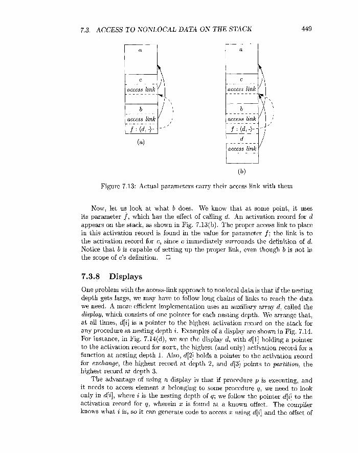
Let us trace what happens when a is executed. First, a calls c, so we place an activation record for c above that for a on the stack. The Access link for c points to the record for a , since c is defined immediately within a. Then c calls b(d). The calling sequence sets up an activation record for b, as shown in Fig. 7.13(a).

Within this activation record is the actual parameter d and its access link, which together form the value of formal parameter f in the activation record for b. Notice that c knows about d, since d is defined within c, and therefore c passes a pointer to its own activation record as the access link. No matter where d was defined, if c is in the scope of that definition, then one of the three rules of Section 7.3.6 must apply, and c can provide the link.


d

access link

C - - - - - - - - - access link

Figure 7.13: Actual parameters carry their access link with them

f : (d, -)- -

Now, let us look at what b does. We know that at some point, it uses its parameter f , which has the effect of calling d. An activation record for d appears on the stack, as shown in Fig. 7.13(b). The proper access link to place in this activation record is found in the value for parameter f; the link is to the activation record for c, since c immediately surrounds the definition of d. Notice that b is capable of setting up the proper link, even though b is not in the scope of c7s definition.

/ - -

7.3.8 Displays

One problem with the access-link approach to nonlocal data is that if the nesting depth gets large, we may have to follow long chains of links to reach the data we need. A more efficient implementation uses an auxiliary array d, called the display, which consists of one pointer for each nesting depth. We arrange that, at all times, d[i] is a pointer to the highest activation record on the stack for any procedure at nesting depth i . Examples of a display are shown in Fig. 7.14. For instance, in Fig. 7.14(d), we see the display d, with d[l] holding a pointer to the activation record for s o r t , the highest (and only) activation record for a function at nesting depth 1. Also, d[2] holds a pointer to the activation record for exchange, the highest record at depth 2, and d[3] points to partition, the highest record at depth 3.

The advantage of using a display is that if procedure p is executing, and it needs to access element x belonging to some procedure q, we need to look only in d[i], where i is the nesting depth of q; we follow the pointer d[i] to the activation record for q, wherein x is found at a known offset. The compiler knows what i is, so it can generate code to access x using d [ i ] and the offset of


Figure 7.14: Maintaining the display

7.3. ACCESS TO NONLOCAL DATA ON THE STACK 451

x from the top of the activation record for q. Thus, the code never needs to follow a long chain of access links.

In order to maintain the display correctly, we need to save previous values of display entries in new activation records. If procedure p at depth n, is called, and its activation record is not the first on the stack for a procedure at depth n,, then the activation record for p needs to hold the previous value of d[np], while d[n,] itself is set to point to this activation of p. When p returns, and its activation record is removed from the stack, we restore d[n,] to have its value prior to the call of p.

Example 7.9: Several steps of manipulating the display are illustrated in Fig. 7.14. In Fig. 7.14(a), sort at depth 1 has called quicksort(1, 9) at depth 2. The activation record for quicksort has a place to store the old value of d[2], indicated as saved d[2], although in this case since there was no prior activation record at depth 2, this pointer is null.

In Fig. 7.14(b), quicksort(1, 9) calls quicksort(l,3). Since the activation records for both calls are at depth 2, we must store the pointer to quicksort(l,9), which was in d[2], in the record for quicksort(l,3). Then, d[2] is made to point to quicksort(173).

Next, partition is called. This function is at depth 3, so we use the slot d[3] in the display for the first time, and make it point to the activation record for partition. The record for partition has a slot for a former value of d[3], but in this case there is none, so the pointer remains null. The display and stack at this time are shown in Fig. 7.14(c).

Then, partition calls exchange. That function is at depth 2, so its activation record stores the old pointer d[2], which goes to the activation record for quicksort(l, 3). Notice that the display pointers "cross"; that is; d[3] points further down the stack than d[2] does. However, that is a proper situation; exchange can only access its own data and that of sort, via d[I].


Exercise 7.3.1 : In Fig. 7.15 is a ML function main that computes Fibonacci numbers in a nonstandard way. Function f ibO will compute the nth Fibonacci number for any n 2 0. Nested within in is f i b l , which computes the nth Fibonacci number on the assumption n > 2, and nested within f i b l is f ib2, which assumes n 2 4. Note that neither f i b l nor f ib2 need to check for the basis cases. Show the stack of activation records that result from a call to main, up until the time that the first call (to f ib0 (1) ) is about to return. Show the access link in each of the activation records on the stack.

Exercise 7.3.2 : Suppose that we implement the functions of Fig. 7.15 using a display. Show the display at the moment the first call to f ib0 (1) is about to return. Also, indicate the saved display entry in each of the activation records on the stack at that time.


fun main () C l e t

fun f ib0 (n) =

l e t fun f i b l ( n ) =

l e t fun f ib2(n) = f ibl(n-1) + f ibl(n-2)

i n i f n >= 4 then f i b2 (n ) e l s e fibO(n-1) + fibO(n-2)

end i n

i f n >= 2 then f i b l ( n ) e l s e 1

end i n

f ib0 (4) end ;

Figure 7.15: Nested functions computing Fibonacci numbers

7.4 Heap Management

The heap is the portion of the store that is used for data that lives indefinitely, or until the program explicitly deletes it. While local variables typically become inaccessible when their procedures end, many languages enable us to create objects or other data whose existence is not tied to the procedure activation that creates them. For example, both C++ and Java give the programmer new to create objects that may be passed - or pointers to them may be passed - from procedure to procedure, so they continue to exist long after the procedure that created them is gone. Such objects are stored on a heap.

In this section, we discuss the memory manager, the subsystem that allocates and deallocates space within the heap; it serves as an interface between application programs and the operating system. For languages like C or C++ that deallocate chunks of storage manually (i.e., by explicit statements of the program, such as f r e e or de l e t e ) , the memory manager is also responsible for implementing deallocation.

In Section 7.5, we discuss garbage collection, which is the process of finding spaces within the heap that are no longer used by the program and can therefore be reallocated to house other data items. For languages like Java, it is the garbage collector that deallocates memory. When it is required, the garbage collector is an important subsystem of the memory manager.

7.4. HEAP MANAGEMENT

7.4.1 The Memory Manager

The memory manager keeps track of all the free space in heap storage at all times. It performs two basic functions:

Allocation. When a program requests memory for a variable or ~ b j e c t , ~ the memory manager produces a chunk of contiguous heap memory of the requested size. If possible, it satisfies an allocation request using free space in the heap; if no chunk of the needed size is available, it seeks to increase the heap storage space by getting consecutive bytes of virtual memory from the operating system. If space is exhausted, the memory manager passes that information back to the application program.

Deallocation. The memory manager returns deallocated space to the pool of free space, so it can reuse the space to satisfy other allocation requests. Memory managers typically do not return memory to the operating system, even if the program's heap usage drops.

Memory management would be simpler if (a) all allocation requests were for chunks of the same size, and (b) storage were released predictably, say, first-allocated first-deallocated. There are some languages, such as Lisp, for which condition (a) holds; pure Lisp uses only one data element - a two- pointer cell - from which all data structures are built. Condition (b) also holds in some situations, the most common being data that can be allocated on the run-time stack. However, in most languages, neither (a) nor (b) holds in general. Rather, data elements of different sizes are allocated, and there is no good way to predict the lifetimes of all allocated objects.

Thus, the memory manager must be prepared to service, in any order, allocation and deallocation requests of any size, ranging from one byte to as large as the program's entire address space.

Here are the properties we desire of memory managers:

Space Efficiency. A memory manager should minimize the total heap space needed by a program. Doing so allows larger programs to run in a fixed virtual address space. Space efficiency is achieved by minimizing "fragmentation," discussed in Section 7.4.4.

Program Efficiency. A memory manager should make good use of the memory subsystem to allow programs to run faster. As we shall see in Section 7.4.2, the time taken to execute an instruction can vary widely depending on where objects are placed in memory. Fortunately, programs tend to exhibit "locality," a phenomenon discussed in Section 7.4.3, which refers to the nonrandom clustered way in which typical programs access memory. By attention to the placement of objects in memory, the memory manager can make better use of space and, hopefully, make the program run faster.

3 ~ n what follows, we shall refer to things requiring memory space as "objects," even if they are not true objects in the "object-oriented programming" sense.

CHAPTER 7. RUN- TIME ENVIRONMENTS

Low Overhead. Because memory allocations and deallocations are fre- quent operations in many programs, it is important that these operations be as efficient as possible. That is, we wish to minimize the overhead - the fraction of execution time spent performing allocation and deallocation. Notice that the cost of allocations is dominated by small requests; the overhead of managing large objects is less important, because it usually can be amortized over a larger amount of computation.

7.4.2 The Memory Hierarchy of a Computer

Memory management and compiler optimization must be done with an aware- ness of how memory behaves. Modern machines are designed,so that programmers can write correct programs without concerning themselves with the details of the memory subsystem. However, the efficiency of a program is determined not just by the number of instructions executed, but also by how long it takes to execute each of these instructions. The time taken to execute an instruction can vary significantly, since the time taken to access different parts of memory can vary from nanoseconds to milliseconds. Data-intensive programs can therefore benefit significantly from optimizations that make good use of the memory subsystem. As we shall see in Section 7.4.3, they can take advantage of the phenomenon of "locality" - the nonrandom behavior of typical programs.

The large variance in memory access times is due to the fundamental limi- tation in hardware technology; we can build small and fast storage, or large and slow storage, but not storage that is both large and fast. It is simply impossible today to build gigabytes of storage with nanosecond access times, which is how fast high-performance processors run. Therefore, practically all modern computers arrange their storage as a memory hierarchy. A memory hierarchy, as shown in Fig. 7.16, consists of a series of storage elements, with the smaller faster ones "closer" to the processor, and the larger slower ones further away.

Typically, a processor has a small number of registers, whose contents are under software control. Next, it has one or more levels of cache, usually made out of static RAM, that are kilobytes to several megabytes in size. The next level of the hierarchy is the physical (main) memory, made out of hundreds of megabytes or gigabytes of dynamic RAM. The physical memory is then backed up by virtual memory, which is implemented by gigabytes of disks. Upon a memory access, the machine first looks for the data in the closest (lowest-level) storage and, if the data is not there, looks in the next higher level, and so on.

Registers are scarce, so register usage is tailored for the specific applications and managed by the code that a compiler generates. All the other levels of the hierarchy are managed automatically; in this way, not only is the programming task simplified, but the same program can work effectively across machines with different memory configurations. With each memory access, the machine searches each level of the memory in succession, starting with the lowest level, until it locates the data. Caches are managed exclusively in hardware, in order to keep up with the relatively fast RAM access times. Because disks are rela-


Typical Sizes Typical Access Times

256MB - 2GB I Physical Memory 1 100 - 150 ns

128KB - 4MB I 2nd-Level Cache 1 40 - 60 ns

3 - 1 5 m s > 2GB

16 - 64KB I 1st-Level Cache I

Virtual Memory (Disk)

Figure 7.16: Typical Memory Hierarchy Configurations

32 Words

tively slow, the virtual memory is managed by the operating system, with the assistance of a hardware structure known as the "translation lookaside buffer."

Data is transferred as blocks of contiguous storage. To amortize the cost of access, larger blocks are used with the slower levels of the hierarchy. Be-

Registers (Processor)

tween main memory and cache, data is transferred in blocks known as cache lines, which are typically from 32 to 256 bytes long. Between virtual memory (disk) and main memory, data is transferred in blocks known as pages, typically between 4K and 64K bytes in size.

1 ns

7.4.3 Locality in Programs

Most programs exhibit a high degree of locality; that is, they spend most of their time executing a relatively small fraction of the code and touching only a small fraction of the data. We say that a program has temporal locality if the memory locations it accesses are likely to be accessed again within a short period of time. We say that a program has spatial locality if memory locations close to the location accessed are likely also to be accessed within a short period of time.

The conventional wisdom is that programs spend 90% of their time executing 10% of the code. Here is why:

Programs often contain many instructions that are never executed. Pro- grams built with components and libraries use only a small fraction of the provided functionality. Also as requirements change and programs evolve, legacy systems often contain many instructions that are no longer used.


Static and Dynamic RAM

Most random-access memory is dynamic, which means that it is built of very simple electronic circuits that lose their charge (and thus "forget" the bit they were storing) in a short time. These circuits need to be refreshed - that is, their bits read and rewritten - periodically. On the other hand, static RAM is designed with a more complex circuit for each bit, and consequently the bit stored can stay indefinitely, until it is changed. Evidently, a chip can store more bits if it uses dynamic-RAM circuits than if it uses static-RAM circuits, so we tend to see large main memories of the dynamic variety, while smaller memories, like caches, are made from static circuits.

Only a small fraction of the code that could be invoked is actually executed in a typical run of the program. For example, instructions to handle illegal inputs and exceptional cases, though critical to the correctness of the program, are seldom invoked on any particular run.

The typical program spends most of its time executing innermost loops and tight recursive cycles in a program.

Locality allows us to take advantage of the memory hierarchy of a modern computer, as shown in Fig. 7.16. By placing the most common instructions and data in the fast-but-small storage, while leaving the rest in the slow-but-large storage, we can lower the average memory-access time of a program significantly.

It has been found that many programs exhibit both temporal and spatial locality in how they access both instructions and data. Data-access patterns, however, generally show a greater variance than instruction-access patterns. Policies such as keeping the most recently used data in the fastest hierarchy work well for common programs but may not work well for some data-intensive programs - ones that cycle through very large arrays, for example.

We often cannot tell, just from looking at the code, which sections of the code will be heavily used, especially for a particular input. Even if we know which instructions are executed heavily, the fastest cache often is not large enough to hold all of them at the same time. We must therefore adjust the contents of the fastest storage dynamically and use it to hold instructions that are likely to be used heavily in the near future.

Optimization Using the Memory Hierarchy

The policy of keeping the most recently used instructions in the cache tends to work well; in other words, the past is generally a good predictor of future memory usage. When a new instruction is executed, there is a high probability that the next instruction also will be executed. This phenomenon is an

7.4. HEAP MANAGEMENT 457

Cache Architectures

How do we know if a cache line is in a cache? It would be too expensive to check every single line in the cache, so it is common practice to restrict the placement of a cache line within the cache. This restriction is known as set associativity. A cache is k-way set associative if a cache line can reside only in k locations. The simplest cache is a 1-way associative cache, also known as a direct-mapped cache. In a direct-mapped cache, data with memory address n can be placed only in cache address n mod s, where s is the size of the cache. Similarly, a k-way set associative cache is divided into k sets, where a datum with address n can be mapped only to the location n mod (slk) in each set. Most instruction and data caches have associativity between 1 and 8. When a cache line is brought into the cache, and all the possible locations that can hold the line are occupied, it is typical to evict the line that has been the least recently used.

example of spatial locality. One effective technique to improve the spatial locality of instructions is to have the compiler place basic blocks (sequences of instructions that are always executed sequentially) that are likely to follow each other contiguously - on the same page, or even the same cache line, if possible. Instructions belonging to the same loop or same function also have a high probability of being executed t ~ g e t h e r . ~

We can also improve the temporal and spatial locality of data accesses in a program by changing the data layout or the order of the computation. For example, programs that visit large amounts of data repeatedly, each time performing a small amount of computation, do not perform well. It is better if we can bring some data from a slow level of the memory hierarchy to a faster level (e.g., disk to main memory) once, and perform all the necessary computations on this data while it resides at the faster level. This concept can be applied recursively to reuse data in physical memory, in the caches and in the registers.

7.4.4 Reducing Fragmentation At the beginning of program execution, the heap is one contiguous unit of free space. As the program allocates and deallocates memory, this space is broken up into free and used chunks of memory, and the free chunks need not reside in a contiguous area of the heap. We refer to the free chunks of memory as holes. With each allocation request, the memory manager must place the requested chunk of memory into a large-enough hole. Unless a hole of exactly the right size is found, we need to split some hole, creating a yet smaller hole.

4 ~ s a machine fetches a word in memory, it is relatively inexpensive to prefetch the next several contiguous words of memory as well. Thus, a common memory-hierarchy feature is that a multiword block is fetched from a level of memory each time that level is accessed.

458 CHAPTER 7. RUN-TIME ENVIRONn(lENTS

With each deallocation request, the freed chunks of memory are added back to the pool of free space. We coalesce contiguous holes into larger holes, as the holes can only get smaller otherwise. If we are not careful, the memory may end up getting fragmented, consisting of large numbers of small, noncontiguous holes. It is then possible that no hole is large enough to satisfy a future request, even though there may be sufficient aggregate free space.

Best-Fit and Next-Fit Object Placement

We reduce fragmentation by controlling how the memory manager places new objects in the heap. It has been found empirically that a good strategy for minimizing fragmentation for real-life programs is to allocate the requested memory in the smallest available hole that is large enough. This best-fit algorithm tends to spare the large holes to satisfy subsequent, larger requests. An alternative, called first-fit, where an object is placed in the first (lowest-address) hole in which it fits, takes less time to place objects, but has been found inferior to best-fit in overall performance.

To implement best-fit placement more efficiently, we can separate free space into bins, according to their sizes. One practical idea is to have many more bins for the smaller sizes, because there are usually many more small objects. For example, the Lea memory manager, used in the GNU C compiler gcc, aligns all chunks to 8-byte boundaries. There is a bin for every multiple of 8-byte chunks from 16 bytes to 512 bytes. Larger-sized bins are logarithmically spaced (i.e., the minimum size for each bin is twice that of the previous bin), and within each of these bins the chunks are ordered by their size. There is always a chunk of free space that can be extended by requesting more pages from the operating system. Called the wilderness chunk, this chunk is treated by Lea as the largest-sized bin because of its extensibility.

Binning makes it easy to find the best-fit chunk.

If, as for small sizes requested from the Lea memory manager, there is a bin for chunks of that size only, we may take any chunk from that bin.

For sizes that do not have a private bin, we find the one bin that is allowed to include chunks of the desired size. Within that bin, we can use either a first-fit or a best-fit strategy; i.e., we either look for and select the first chunk that is sufficiently large or, we spend more time and find the smallest chunk that is sufficiently large. Note that when the fit is not exact, the remainder of the chunk will generally need to be placed in a bin with smaller sizes.

However, it may be that the target bin is empty, or all chunks in that bin are too small to satisfy the request for space. In that case, we simply repeat the search, using the bin for the next larger size(s). Eventually, we either find a chunk we can use, or we reach the "wilderness7' chunk, from which we can surely obtain the needed space, possibly by going to the operating system and getting additional pages for the heap.

7.4. HEAP MANAGEMENT 459

While best-fit placement tends to improve space utilization, it may not be the best in terms of spatial locality. Chunks allocated at about the same time by a program tend to have similar reference patterns and to have similar lifetimes. Placing them close together thus improves the program's spatial locality. One useful adaptation of the best-fit algorithm is to modify the placement in the case when a chunk of the exact requested size cannot be found. In this case, we use a next-fit strategy, trying to allocate the object in the chunk that has last been split, whenever enough space for the new object remains in that chunk. Next-fit also tends to improve the speed of the allocation operation.

Managing and Coalescing Free Space

When an object is deallocated manually, the memory manager must make its chunk free, so it can be allocated again. In some circumstances, it may also be possible to combine (coalesce) that chunk with adjacent chunks of the heap, to form a larger chunk. There is an advantage to doing so, since we can always use a large chunk to do the work of small chunks of equal total size, but many small chunks cannot hold one large object, as the combined chunk could.

If we keep a bin for chunks of one fixed size, as Lea does for small sizes, then we may prefer not to coalesce adjacent blocks of that size into a chunk of double the size. It is simpler to keep all the chunks of one size in as many pages as we need, and never coalesce them. Then, a simple allocation/deallocation scheme is to keep a bitmap, with one bit for each chunk in the bin. A 1 indicates the chunk is occupied; 0 indicates it is free. When a chunk is deallocated, we change its 1 to a 0. When we need to allocate a chunk, we find any chunk with a 0 bit, change that bit to a I, and use the corresponding chunk. If there are no free chunks, we get a new page, divide it into chunks of the appropriate size, and extend the bit vector.

Matters are more complex when the heap is managed as a whole, without binning, or if we are willing to coalesce adjacent chunks and move the resulting chunk to a different bin if necessary. There are two data structures that are useful to support coalescing of adjacent free blocks:

Boundary Tags. At both the low and high ends of each chunk, whether free or allocated, m7e keep vital information. At both ends, we keep a free/used bit that tells whether or not the block is currently allocated (used) or available (free). Adjacent to each free/used bit is a count of the total number of bytes in the chunk.

A Doubly Linked, Embedded Free List. The free chunks (but not the allocated chunks) are also linked in a doubly linked list. The pointers for this list are within the blocks themselves, say adjacent to the boundary tags at either end. Thus, no additional space is needed for the free list, although its existence does place a lower bound on how small chunks can get; they must accommodate two boundary tags and two pointers, even if the object is a single byte. The order of chunks on the free list is left


unspecified. For example, the list could be sorted by size, thus facilitating best-fit placement.

Example 7.10 : Figure 7.17 shows part of a heap with three adjacent chunks, A, B , and C. Chunk B , of size 100, has just been deallocated and returned to the free list. Since we know the beginning (left end) of B , we also know the end of the chunk that happens to be immediately to B's left, namely A in this example. The freelused bit at the right end of A is currently 0, so A too is free. We may therefore coalesce A and B into one chunk of 300 bytes.

Chunk A Chunk B Chunk C

Figure 7.17: Part of a heap and a doubly linked free list

It might be the case that chunk C, the chunk immediately to B's right, is also free, in which case we can combine all of A, B , and C. Note that if we always coalesce chunks when we can, then there can never be two adjacent free chunks, so we never have to look further than the two chunks adjacent to the one being deallocated. In the current case, we find the beginning of C by starting at the left end of B, which we know, and finding the total number of bytes in B, which is found in the left boundary tag of B and is 100 bytes. With this information, we find the right end of B and the beginning of the chunk to its right. At that point, we examine the freelused bit of C and find that it is 1 for used; hence, C is not available for coalescing.

Since we must coalesce A and B , we need to remove one of them from the free list. The doubly linked free-list structure lets us find the chunks before and after each of A and B. Notice that it should not be assumed that physical neighbors A and B are also adjacent on the free list. Knowing the chunks preceding and following A and B on the free list, it is straightforward to manipulate pointers on the list to replace A and B by one coalesced chunk.

Automatic garbage collection can eliminate fragmentation altogether if it moves all the allocated objects to contiguous storage. The interaction between garbage collection and memory management is discussed in more detail in Sec- tion 7.6.4.

7.4.5 Manual Deallocation Requests

We close this section with manual memory management, where the programmer must explicitly arrange for the deallocation of data, as in C and C++. Ideally, any storage that will no longer be accessed should be deleted. Conversely, any storage that may be referenced must not be deleted. Unfortunately, it is hard to enforce either of these properties. In addition to considering the difficulties with


manual deallocation, we shall describe some of the techniques programmers use to help with the difficulties.

Problems with Manual Deallocation

Manual memory management is error-prone. The common mistakes take two forms: failing ever to delete data that cannot be referenced is called a rnernory- leak error, and referencing deleted data is a dangling-pointer-dereference error.

It is hard for programmers to tell if a program will never refer to some storage in the future, so the first common mistake is not deleting storage that will never be referenced. Note that although memory leaks may slow down the execution of a program due to increased memory usage, they do not affect program correctness, as long as the machine does not run out of memory. Many programs can tolerate memory leaks, especially if the leakage is slow. However, for long-running programs, and especially nonstop programs like operating systems or server code, it is critical that they not have leaks.

Automatic garbage collection gets rid of memory leaks by deallocating all the garbage. Even with automatic garbage collection, a program may still use more memory than necessary. A programmer may know that an object will never be referenced, even though references to that object exist somewhere. In that case, the programmer must deliberately remove references to objects that will never be referenced, so the objects can be deallocated automatically.

Being overly zealous about deleting objects can lead to even worse problems than memory leaks. The second common mistake is to delete some storage and then try to refer to the data in the deallocated storage. Pointers to storage that has been deallocated are known as dangling pointers. Once the freed storage has been reallocated to a new variable, any read, write, or deallocation via the dangling pointer can produce seemingly random effects. We refer to any operation, such as read, write, or deallocate, that follows a pointer and tries to use the object it points to, as dereferencing the pointer.

Notice that reading through a dangling pointer may return an arbitrary value. Writing through a dangling pointer arbitrarily changes the value of the new variable. Deallocating a dangling pointer's storage means that the storage of the new variable may be allocated to yet another variable, and actions on the old and new variables may conflict with each other.

Unlike memory leaks, dereferencing a dangling pointer after the freed storage is reallocated almost always creates a program error that is hard to debug. As a result, programmers are more inclined not to deallocate a variable if they are not certain it is unreferencable.

A related form of programming error is to access an illegal .address. Common examples of such errors include dereferencing null pointers and accessing an out-of-bounds array element. It is better for such errors to be detected than to have the program silently corrupt the results. In fact, many security violations exploit programming errors of this type, where certain program inputs allow unintended access to data, leading to a "hacker" taking control of the program


An Example: Purify

Rational's Purify is one of the most popular commercial tools that helps programmers find memory access errors and memory leaks in programs. Purify instruments binary code by adding additional instructions to check for errors as the program executes. It keeps a map of memory to indicate where all the freed and used spaces are. Each allocated object is bracketed with extra space; accesses to unallocated locations or to spaces between objects are flagged as errors. This approach finds some dangling pointer references, but not when the memory has been reallocated and a valid object is sitting in its place. This approach also finds some out-of-bound array accesses, if they happen to land in the space inserted at the end of the objects.

Purify also finds memory leaks at the end of a program execution. It searches the contents of all the allocated objects for possible pointer values. Any object without a pointer to it is a leaked chunk of memory. Purify reports the amount of memory leaked and the locations of the leaked objects. We may compare Purify to a "conservative garbage collector," which will be discussed in Section 7.8.3.

and machine. One antidote is to have the compiler insert checks with every access, to make sure it is within bounds. The compiler's optimizer can discover and remove those checks that are not really necessary because the optimizer can deduce that the access must be within bounds.

Programming Conventions and Tools

We now present a few of the most popular conventions and tools that have been developed to help programmers cope with the complexity in managing memory:

Object ownership is useful when an object's lifetime can be statically rea- soned about. The idea is to associate an owner with each object at all times. The owner is a pointer to that object, presumably belonging to some function invocation. The owner (i.e., its function) is responsible for either deleting the object or for passing the object to another owner. It is possible to have other, nonowning pointers to the same object; these pointers can be overwritten any time, and no deletes should ever be applied through them. This convention eliminates memory leaks, as well as attempts to delete the same object twice. However, it does not help solve the dangling-pointer-reference problem, because it is possible to follow a nonowning pointer to an object that has been deleted.

Reference counting is useful when an object's lifetime needs to be determined dynamically. The idea is to associate a count with each dynamically

7.5. INTRODUCTION TO GARBAGE COLLECTION 463

allocated object. Whenever a reference to the object is created, we increment the reference count; whenever a reference is removed, we decrement the reference count. When the count goes to zero, the object can no longer be referenced and can therefore be deleted. This technique, however, does not catch useless, circular data structures, where a collection of objects cannot be accessed, but their reference counts are not zero, since they refer to each other. For an illustration of this problem, see Example 7.11. Reference counting does eradicate all dangling-pointer references, since there are no outstanding references to any deleted objects. Reference counting is expensive because it imposes an overhead on every operation that stores a pointer.

Region-based allocation is useful for collections of objects whose lifetimes are tied to specific phases in a computation.When objects are created to be used only within some step of a computation, we can allocate all such objects in the same region. We then delete the entire region once that computation step completes. This region-based allocation technique has limited applicability. However, it is very efficient whenever it can be used; instead of deallocating objects one at a time, it deletes all objects in the region in a wholesale fashion.


Exercise 7.4.1 : Suppose the heap consists of seven chunks, starting at address 0. The sizes of the chunks, in order, are 80, 30, 60, 50, 70, 20, 40 bytes. When we place an object in a chunk, we put it at the high end if there is enough space remaining to form a smaller chunk (so that the smaller chunk can easily remain on the linked list of free space). However, we cannot tolerate chunks of fewer that 8 bytes, so if an object is almost as large as the selected chunk, we give it the entire chunk and place the object at the low end of the chunk. If we request space for objects of the following sizes: 32, 64, 48, 16, in that order, what does the free space list look like after satisfying the requests, if the method of selecting chunks is

a) First fit.

b) Best fit.

7.5 Introduction to Garbage Collection

Data that cannot be referenced is generally known as garbage. Many high-level programming languages remove the burden of manual memory management from the programmer by offering automatic garbage collection, which deallocates unreachable data. Garbage collection dates back to the initial implementation of Lisp in 1958. Other significant languages that offer garbage collection include Java, Perl, ML, Modula-3, Prolog, and Smalltalk.


In this section, we introduce many of the concepts of garbage collection. The notion of an object being "reachable" is perhaps intuitive, but we need to be precise; the exact rules are discussed in Section 7.5.2. We also discuss, in Section 7.5.3, a simple, but imperfect, method of automatic garbage collection: reference counting, which is based on the idea that once a program has lost all references to an object, it simply cannot and so will not reference the storage.

Section 7.6 covers trace-based collectors, which are algorithms that discover all the objects that are still useful, and then turn all the other chunks of the heap into free space.

7.5.1 Design Goals for Garbage Collectors

Garbage collection is the reclamation of chunks of storage holding objects that can no longer be accessed by a program. We need to assume that objects have a type that can be determined by the garbage collector at run time. From the type information, we can tell how large the object is and which components of the object contain references (pointers) to other objects. We also assume that references to objects are always to the address of the beginning of the object, never pointers to places within the object. Thus, all references to an object have the same value and can be identified easily.

A user program, which we shall refer to as the mutator, modifies the collection of objects in the heap. The mutator creates objects by acquiring space from the memory manager, and the mutator may introduce and drop references to existing objects. Objects become garbage when the mutator program cannot "reach77 them, in the sense made precise in Section 7.5.2. The garbage collector finds these unreachable objects and reclaims their space by handing them to the memory manager, which keeps track of the free space.

A Basic Requirement: Type Safety

Not all languages are good candidates for automatic garbage collection. For a garbage collector to work, it must be able to tell whether any given data element or component of a data element is, or could be used as, a pointer to a chunk of allocated memory space. A language in which the type of any data component can be determined is said to be type safe. There are type-safe languages like ML, for which we can determine types at compile time. There are other type- safe languages, like Java, whose types cannot be determined at compile time, but can be determined at run time. The latter are called dynamically typed languages. If a language is neither statically nor dynamically type safe, then it is said to be unsafe.

Unsafe languages, which unfortunately include some of the most important languages such as C and C++, are bad candidates for automatic garbage collection. In unsafe languages, memory addresses can be manipulated arbitrarily: arbitrary arithmetic operations can be applied to pointers to create new pointers, and arbitrary integers can be cast as pointers. Thus a program

7.5. INTRODUCTION TO GARBAGE COLLECTION

theoretically could refer to any location in memory at any time. Consequently, no memory location can be considered to be inaccessible, and no storage can ever: be reclaimed safely.

In practice, most C and C++ programs do not generate pointers arbitrarily, and a theoretically unsound garbage collector that works well empirically has been developed and used. We shall discuss conservative garbage collection for C and C++ in Section 7.8.3.

Performance Metrics

Garbage collection is often so expensive that, although it was invented decades ago and absolutely prevents memory leaks, it has yet to be adopted by many mainstream programming languages. Many different approaches have been proposed over the years, and there is not one clearly best garbage-collection algorithm. Before exploring the options, let us first enumerate the performance metrics that must be considered when designing a garbage collector.

Overall Execution Time. Garbage collection can be very slow. It is important that it not significantly increase the total run time of an application. Since the garbage collector necessarily must touch a lot of data, its performance is determined greatly by how it leverages the memory subsystem.

Spa& Usage. It is important that garbage collection avoid fragmentation and make the best use of the available memory.

Pause Time. Simple garbage collectors are notorious for causing programs - the mutators - to pause suddenly for an extremely long time, as garbage collection kicks in without warning. Thus, besides minimizing the overall execution time, it is desirable that the maximum pause time be minimized. As an important special case, real-time applications require certain computations to be completed within a time limit. We must either suppress garbage collection while performing real-time tasks, or restrict maximum pause time. Thus, garbage collection is seldom used in real-time applications.

Program Locality. We cannot evaluate the speed of a garbage collector solely by its running time. The garbage collector controls the placement of data and thus influences the data locality of the mutator program. It can improve a mutator's temporal locality by freeing up space and reusing it; it can improve the mutator's spatial locality by relocating data used together in the same cache or pages.

Some of these design goals conflict with one another, and tradeoffs must be made carefully by considering how programs typically behave. Also objects of different characteristics may favor different treatments, requiring a collector to use different techniques for different kinds of objects.


For example, the number of objects allocated is dominated by small objects, so allocation of small objects must not incur a large overhead. On the other hand, consider garbage collectors that relocate reachable objects. Relocation is expensive when dealing with large objects, but less so with small objects.

As another example, in general, the longer we wait to collect garbage in a trace-based collector, the larger the fraction of objects that can be collected. The reason is that objects often "die young," so if we wait a while, many of the newly allocated objects will become unreachable. Such a collector thus costs less on the average, per unreachable object collected. On the other hand, infrequent collection increases a program's memory usage, decreases its data locality, and increases the length of the pauses.

In contrast, a reference-counting collector, by introducing a constant overhead to many of the mutator's operations, can slow down the overall execution of a program significantly. On the other hand, reference counting does not create long pauses, and it is memory efficient, because it finds garbage as soon as it is produced (with the exception of certain cyclic structures discussed in Section 7.5.3).

Language design can also affect the characteristics of memory usage. Some languages encourage a programming style that generates a lot of garbage. For example, programs in functional or almost functional programming languages create more objects to avoid mutating existing objects. In Java, all objects, other than base types like integers and references, are allocated on the heap and not the stack, even if their lifetimes are confined to that of one function invocation. This design frees the programmer from worrying about the lifetimes of variables, at the expense of generating more garbage. Compiler optimizations have been developed to analyze the lifetimes of variables and allocate them on the stack whenever possible.

7.5.2 Reachability

We refer to all the data that can be accessed directly by a program, without having to dereference any pointer, as the root set. For example, in Java the root set of a program consists of all the static field members and all the variables on its stack. A program obviously can reach any member of its root set at any time. Recursively, any object with a reference that is stored in the field members or array elements of any reachable object is itself reachable.

Reachability becomes a bit more complex when the program has been op- timized by the compiler. First, a compiler may keep reference variables in registers. These references must also be considered part of the root set. Sec- ond, even though in a type-safe language programmers do not get to manipulate memory addresses directly, a compiler often does so for the sake of speeding up the code. Thus, registers in compiled code may point to the middle of an object or an array, or they may contain a value to which an offset will be applied to compute a legal address. Here are some things an optimizing compiler can do to enable the garbage collector to find the correct root set:

7.5. INTRODUCTION TO GARBAGE COLLECTION

The compiler can restrict the invocation of garbage collection to only certain code points in the program, when no "hidden" references exist.

The compiler can write out information that the garbage collector can use to recover all the references, such as specifying which registers contain references, or how to compute the base address of an object that is given an internal address.

The compiler can assure that there is a reference to the base address of all reachable objects whenever the garbage collector may be invoked.

The set of reachable objects changes as a program executes. It grows as new objects get created and shrinks as objects become unreachable. It is important to remember that once an object becomes unreachable, it cannot become reachable again. There are four basic operations that a mutator performs to change the set of reachable objects:

Object Allocations. These are performed by the memory manager, which returns a reference to each newly allocated chunk of memory. This operation adds members to the set of reachable objects.

Parameter Passing and Return Values. References to objects are passed from the actual input parameter to the corresponding formal parameter, and from the returned result back to the callee. Objects pointed to by these references remain reachable.

Reference Assignments. Assignments of the form u = v, where u and v are references, have two effects. First, u is now a reference to the object referred to by v. As long as u is reachable, the object it refers to is surely reachable. Second, the original reference in u is lost. If this reference is the last to some reachable object, then that object becomes unreachable. Any time an object becomes unreachable, all objects that are reachable only through references contained in that object also become unreachable.

Procedure Returns. As a procedure exits, the frame holding its local variables is popped off the stack. If the frame holds the only reachable reference to any object, that object becomes unreachable. Again, if the now unreachable objects hold the only references to other objects, they too become unreachable, and so on.

In summary, new objects are introduced through object allocations. Param- eter passing and assignments can propagate reachability; assignments and ends of procedures can terminate reachability. As an object becomes unreachable, it can cause more objects to become unreachable.

There are two basic ways to find unreachable objects. Either we catch the transitions as reachable objects turn unreachable, or we periodically locate all the reachable objects and then infer that all the other objects are unreachable. Reference counting, introduced in Section 7.4.5, is a well-known approximation


Survival of Stack Objects

When a procedure is called, a local variable v, whose object is allocated on the stack, may have pointers to v placed in nonlocal variables. These pointers will continue to exist after the procedure returns, yet the space for v disappears, resulting in a dangling-reference situation. Should we ever allocate a local like v on the stack, as C does for example? The answer is that the semantics of many languages requires that local variables cease to exist when their procedure returns. Retaining a reference to such a variable is a programming error, and the compiler is not required to fix the bug in the program.

to the first approach. We maintain a count of the references to an object, as the mutator performs actions that may change the reachability set. When the count goes to zero, the object becomes unreachable. We discuss this approach in more detail in Section 7.5.3.

The second approach computes reachability by tracing all the references transitively. A trace-based garbage collector starts by labeling ("marking") all objects in the root set as "reachable," examines iteratively all the references in reachable objects to find more reachable objects, and labels them as such. This approach must trace all the references before it can determine any object to be unreachable. But once the reachable set is computed, it can find many unreachable objects all at once and locate a good deal of free storage at the same time. Because all the references must be analyzed at the same time, we have an option to relocate the reachable objects and thereby reduce fragmentation. There are many different trace-based algorithms, and we discuss the options in Sections 7.6 and 7.7.1.

7.5.3 Reference Counting Garbage Collectors We now consider a simple, although imperfect, garbage collector, based on reference counting, which identifies garbage as an object changes from being reachable to unreachable; the object can be deleted when its count drops to zero. With a reference-counting garbage collector, every object must have a field for the reference count. Reference counts can be maintained as follows:

1. Object Allocation. The reference count of the new object is set to 1.

2. Parameter Passing. The reference count of each object passed into a procedure is incremented.

3. Reference Assignments. For statement u = v, where u and v are references, the reference count of the object referred to by v goes up by one, and the count for the old object referred to by u goes down by one.

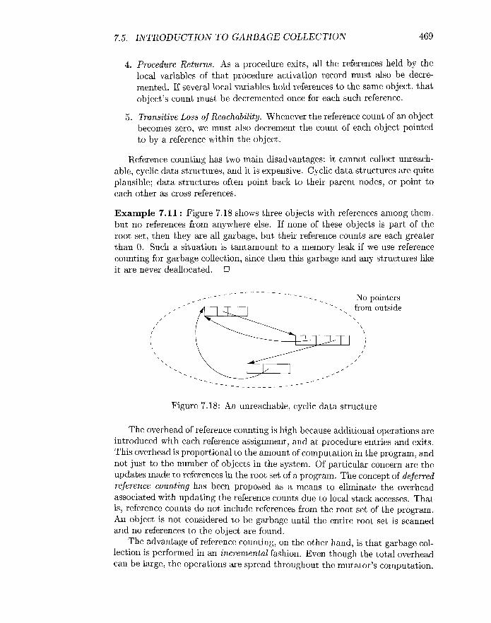
7.5. INTRODUCTION TO GARBAGE COLLECTION 469

4. Procedure Returns. As a procedure exits, all the references held by the local variables of that procedure activation record must also be decremented. If several local variables hold references to the same object, that object's count must be decremented once for each such reference.

5. Transitive Loss of Reachability. Whenever the reference count of an object becomes zero, we must also decrement the count of each object pointed to by a reference within the object.

Reference counting has two main disadvantages: it cannot collect unreachable, cyclic data structures, and it is expensive. Cyclic data structures are quite plausible; data structures often point back to their parent nodes, or point to each other as cross references.

Example 7.11 : Figure 7.18 shows three objects with references among them, but no references from anywhere else. If none of these objects is part of the root set, then they are all garbage, but their reference counts are each greater than 0. Such a situation is tantamount to a memory leak if we use reference counting for garbage collection, since then this garbage and any structures like it are never deallocated.

_ - - - - - - - - - - - - - - - No pointers outside

Figure 7.18: An unreachable, cyclic data structure

The overhead of reference counting is high because additional operations are introduced with each reference assignment, and at procedure entries and exits. This overhead is proportional to the amount of computation in the program, and not just to the number of objects in the system. Of particular concern are the updates made to references in the root set of a program. The concept of deferred reference counting has been proposed as a means to eliminate the overhead associated with updating the reference counts due to local stack accesses. That is, reference counts do not include references from the root set of the program. An object is not considered to be garbage until the entire root set is scanned and no references to the object are found.

The advantage of reference counting, on the other hand, is that garbage collection is performed in an incremental fashion. Even though the total overhead can be large, the operations are spread throughout the mutator's computation.


Although removing one reference may render a large number of objects unreachable, the operation of recursively modifying reference counts can easily be deferred and performed piecemeal across time. Thus, reference counting is particularly attractive algorithm when timing deadlines must be met, as well as for interactive applications where long, sudden pauses are unacceptable. Another advantage is that garbage is collected immediately, keeping space usage low.

Figure 7.19: A network of objects


Exercise 7.5.1 : What happens to the reference counts of the objects in Fig. 7.19 if:

a) The pointer from A to B is deleted.

b) The pointer from X to A is deleted.

c) The node C is deleted.

Exercise 7.5.2 : What happens to reference counts when the pointer from A to D in Fig. 7.20 is deleted?

7.6 Introduction to Trace-Based Collection

Instead of collecting garbage as it is created, trace-based collectors run periodically to find unreachable objects and reclaim their space. Typically, we run the

7.6. INTRODUCTION TO TRACE-BASED COLLECTION

Figure 7.20: Another network of objects

trace-based collector whenever the free space is exhausted or its amount drops below some threshold.

We begin this section by introducing the simplest "mark-and-sweep" garbage collection algorithm. We then describe the variety of trace-based algorithms in terms of four states that chunks of memory can be put in. This section also contains a number of improvements on the basic algorithm, including those in which object relocation is a part of the garbage-collection function.

7.6.1 A Basic Mark-and-Sweep Collector

Mark-and-sweep garbage-collection algorithms are straightforward, stop-the- world algorithms that find all the unreachable objects, and put them on the list of free space. Algorithm 7.12 visits and "marks" all the reachable objects in the first tracing step and then "sweeps" the entire heap to free up unreachable objects. Algorithm 7.14, which we consider after introducing a general framework for trace-based algorithms, is an optimization of Algorithm 7.12. By using an additional list to hold all the allocated objects, it visits the reachable objects only once.

Algorithm 7.12 : Mark-and-sweep garbage collection.

INPUT: A root set of objects, a heap, and a free list, called Free, with all the unallocated chunks of the heap. As in Section 7.4.4, all chunks of space are marked with boundary tags to indicate their free/used status and size.

OUTPUT: A modified Free list after all the garbage has been removed.

METHOD: The algorithm, shown in Fig. 7.21, uses several simple data structures. List Free holds objects known to be free. A list called Unscanned, holds objects that we have determined are reached, but whose successors we have not yet considered. That is, we have not scanned these objects to see what other

CHAPTER 7. RUN-TME ENVIRONMENTS

/* marking phase */ set the reached-bit to 1 and add to list Unscanned each object

referenced by the root set; while ( Unscanned # 0) {

remove some object o from Unscanned; for (each object o' referenced in o) {

if (0' is unreached; i.e., its reached-bit is 0) { set the reached-bit of o' to 1; put o' in Unscanned;

1 I

I /* sweeping phase */ Free = 0; for (each chunk of memory o in the heap) {

if (o is unreached, i.e., its reached-bit is 0) add o to Free; else set the reached-bit of o to 0;

3

Figure 7.21: A Mark-and-Sweep Garbage Collector

objects can be reached through them. The Unscanned list is empty initially. Additionally, each object includes a bit to indicate whether it has been reached (the reached- bit). Before the algorithm begins, all allocated objects have the reached-bit set to 0.

In line (1) of Fig. 7.21, we initialize the Unscanned list by placing there all the objects referenced by the root set. The reached-bit for these objects is also set to 1. Lines (2) through (7) are a loop, in which we, in turn, examine each object o that is ever placed on the Unscanned list.

The for-loop of lines (4) through (7) implements the scanning of object o. We examine each object o' for which we find a reference within o. If o' has already been reached (its reached-bit is I) , then there is no need to do anything about 0'; it either has been scanned previously, or it is on the Unscanned list to be scanned later. However, if o' was not reached already, then we need to set its reached-bit to 1 in line (6) and add o' to the Unscanned list in line (7). Figure 7.22 illustrates this process. It shows an Unscanned list with four objects. The first object on this list, corresponding to object o in the discussion above, is in the process of being scanned. The dashed lines correspond to the three kinds of objects that might be reached from o:

1. A previously scanned object that need not be scanned again.

2. An object currently on the Unscanned list.

3. An item that is reachable, but was previously thought to be unreached.

7.6. INTRODUCTION TO TRACE-BASED COLLECTION

Free and unreached objects reached bit = 0

Unscanned and previously scanned objects reached bit = 1

Figure 7.22: The relationships among objects during the marking phase of a mark-and-sweep garbage collector

Lines (8) through (ll), the sweeping phase, reclaim the space of all the objects that remain unreached at the end of the marking phase. Note that these will include any objects that were on the Free list originally. Because the set of unreached objects cannot be enumerated directly, the algorithm sweeps through the entire heap. Line (10) puts free and unreached objects on the Free list, one at a time. Line (11) handles the reachable objects. We set their reached-bit to 0, in order to maintain the proper preconditions for the next execution of the garbage-collection algorithm.

7.6.2 Basic Abstraction

All trace-based algorithms compute the set of reachable objects and then take the complement of this set. Memory is therefore recycled as follows:

a) The program or mutator runs and makes allocation requests.

b) The garbage collector discovers reachability by tracing.

c) The garbage collector reclaims the storage for unreachable objects.

This cycle is illustrated in Fig. 7.23 in terms of four states for chunks of memory: Free, Unreached, Unscanned, and Scanned. The state of a chunk might be stored in the chunk itself, or it might be implicit in the data structures used by the garbage-collection algorithm.

While trace- based algorithms may differ in their implement ation, they can all be described in terms of the following states:

1. Free. A chunk is in the Free state if it is ready to be allocated. Thus, a Free chunk must not hold a reachable object.

2. Unreached. Chunks are presumed unreachable, unless proven reachable by tracing. A chunk is in the Unreached state at any point during garbage

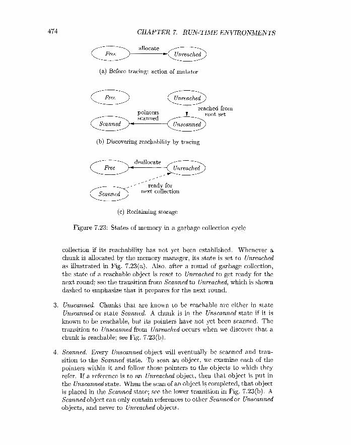
CHAPTER 7. RUN-'TIME ENVIRONMENTS

allocate Free

(a) Before tracing: action of mutator

pointers root set

(b) Discovering reachability by tracing

- - ' ready for next collection

(c) Reclaiming storage

Figure 7.23: States of memory in a garbage collection cycle

collection if its reachability has not yet been established. Whenever a chunk is allocated by the memory manager, its state is set to Unreached as illustrated in Fig. 7.23(a). Also, after a round of garbage collection, the state of a reachable object is reset to Unreached to get ready for the next round; see the transition from Scanned to Unreached, which is shown dashed to emphasize that it prepares for the next round.

3. Unscanned, Chunks that are known to be reachable are either in state Unscanned or state Scanned. A chunk is in the Unscanned state if it is known to be reachable, but its pointers have not yet been scanned. The transition to Unscanned from Unreached occurs when we discover that a chunk is reachable; see Fig. 7.23(b).

4. Scanned. Every Unscanned object will eventually be scanned and transition to the Scanned state. To scan an object, we examine each of the pointers within it and follow those pointers to the objects to which they refer. If a reference is to an Unreached object, then that object is put in the Unscanned state. When the scan of an object is completed, that object is placed in the Scanned state; see the lower transition in Fig. 7.23(b). A Scanned object can only contain references to other Scanned or Unscanned objects, and never to Unreached objects.

7.6. INTRODUCTION TO TRACE-BASED COLLECTION 475

When no objects are left in the Unscanned state, the computation of reachability is complete. Objects left in the Unreached state at the end are truly unreachable. The garbage collector reclaims the space they occupy and places the chunks in the Free state, as illustrated by the solid transition in Fig. 7.23(c). To get ready for the next cycle of garbage collection, objects in the Scanned state are returned to the Unreached state; see the dashed transition in Fig. 7.23(c). Again, remember that these objects really are reachable right now. The Un- reachable state is appropriate because we shall want to start all objects out in this state when garbage collection next begins, by which time any of the currently reachable objects may indeed have been rendered unreachable.

Example 7.13: Let us see how the data structures of Algorithm 7.12 relate to the four states introduced above. Using the reached-bit and membership on lists Free and Unscanned, we can distinguish among all four states. The table of Fig. 7.24 summarizes the characterization of the four states in terms of the data structure for Algorithm 7.12.

Figure 7.24: Representation of states in Algorithm 7.12

STATE Free Unreached Unscanned Scanned

7.6.3 Optimizing Mark-and-Sweep

ON Free ON Unscanned REACHED-BIT Yes No 0 No No 0 No Yes 1 No No 1

The final step in the basic mark-and-sweep algorithm is expensive because there is no easy way to find only the unreachable objects without examining the entire heap. An improved algorithm, due to Baker, keeps a list of all allocated objects. To find the set of unreachable objects, which we must return to free space, we take the set difference of the allocated objects and the reached objects.

Algorithm 7.14 : Baker's mark-and-sweep collector. \

INPUT: A root set of objects, a heap, a free list Free, and a list of allocated objects, which we refer to as Unreached.

OUTPUT: Modified lists Free and Unreached, which holds allocated objects.

METHOD: In this algorithm, shown in Fig. 7.25, the data structure for garbage collection is four lists named Free, Unreached, Unscanned, and Scanned, each of which holds all the objects in the state of the same name. These lists may be implemented by embedded, doubly linked lists, as was discussed in Sec- tion 7.4.4. A reached-bit in objects is not used, but we assume that each object


contains bits telling which of the four states it is in. Initially, Free is the free list maintained by the memory manager, and all allocated objects are on the Unreached list (also maintained by the memory manager as it allocates chunks to objects).

I) Scanned = 0; 2) Unscanned = set of objects referenced in the root set;

3) while (Unscanned # 0) { 4) move object o from Unscanned to Scanned; 5) for (each object o' referenced in o) { 6) if (0' is in Unreached) 7 ) move o' from Unreached to Unscanned;

1 1

8) Free = Free U Unreached; 9) Unreached = Scanned;

Figure 7.25: Baker's mark-and-sweep algorithm

Lines (1) and (2) initialize Scanned to be the empty list, and Unscanned to have only the objects reached from the root set. Note that these objects were presumably on the list Unreached and must be removed from there. Lines (3) through (7) are a straightforward implementation of the basic marking algorithm, using these lists. That is, the for-loop of lines (5) through (7) examines the references in one unscanned object o, and if any of those references o' have not yet been reached, line (7) changes o' to the Unscanned state.

At the end, line (8) takes those objects that are still on the Unreached list and deallocates their chunks, by moving them to the Free list. Then, line (9) takes all the objects in state Scanned, which are the reachable objects, and reinitializes the Unreached list to be exactly those objects. Presumably, as the memory manager creates new objects, those too will be added to the Unreached list and removed from the Free list.

In both algorithms of this section, we have assumed that chunks returned to the free list remain as they were before deallocation. However, as discussed in Section 7.4.4, it is often advantageous to combine adjacent free chunks into larger chunks. If we wish to do so, then every time we return a chunk to the free list, either at line (10) of Fig. 7.21 or line (8) of Fig. 7.25, we examine the chunks to its left and right, and merge if one is free.

7.6.4 Mark-and-Compact Garbage Collectors

Relocating collectors move reachable objects around in the heap to eliminate memory fragmentation. It is common that the space occupied by reachable objects is much smaller than the freed space. Thus, after identifying all the holes,

7.6. INTRODUCTION T O TRACE-BASED COLLECTION 477

instead of freeing them individually, one attractive alternative is to relocate all the reachable objects into one end of the heap, leaving the entire rest of the heap as one free chunk. After all, the garbage collector has already analyzed every reference within the reachable objects, so updating them to point to the new locations does not require much more work. These, plus the references in the root set, are all the references we need to change.

Having all the reachable objects in contiguous locations reduces fragmentation of the memory space, making it easier to house large objects. Also, by making the data occupy fewer cache lines and pages, relocation improves a program's temporal and spatial locality, since new objects created at about the same time are allocated nearby chunks. Objects in nearby chunks can benefit from prefetching if they are used together. Further, the data structure for maintaining free space is simplified; instead of a free list, all we need is a pointer free to the beginning of the one free block.

Relocating collectors vary in whether they relocate in place or reserve space ahead of time for the relocation:

A mark-and-compact collector, described in this section, compacts objects in place. Relocating in place reduces memory usage.

The more efficient and popular copying collector in Section 7.6.5 moves objects from one region of memory to another. Reserving extra space for relocation allows reachable objects to be moved as they are discovered.

The mark-and-compact collector in Algorithm 7.15 has three phases:

1. First is a marking phase, similar to that of the mark-and-sweep algorithms described previously.

2. Second, the algorithm scans the allocated section of the heap and computes a new address for each of the reachable objects. New addresses are assigned from the low end of the heap, so there are no holes between reachable objects. The new address for each object is recorded in a structure called NewLocation.

3. Finally, the algorithm copies objects to their new locations, updating all references in the objects to point to the corresponding new locations. The needed addresses are found in NewLocation.

Algorithm 7.15 : A mark-and-compact garbage collector.

INPUT: A root set of objects, a heap, and free, a pointer marking the start of free space.

OUTPUT: The new value of pointer free.

METHOD: The algorithm is in Fig. 7.26; it uses the following data structures:

1. An Unscanned list, as in Algorithm 7.12.


2. Reached bits in all objects, also as in Algorithm 7.12. To keep our description simple, we refer to objects as "reached" or "unreached," when we mean that their reached-bit is 1 or 0, respectively. Initially, all objects are unreached.

3. The pointer free, which marks the beginning of undlocated space in the heap.

4. The table NewLocation. This structure could be a hash table, search tree, or another structure that implements the two operations:

(a) Set NewLocation(o) to a new address for object o.

(b) Given object o, get the value of NewLocation(o).

We shall not concern ourselves with the exact structure used, although you may assume that NewLocation is a hash table, and therefore, the "set" and "get" operations are each performed in average constant time, independent of how many objects are in the heap.

The first, or marking, phase of lines (I) through (7) is essentially the same as the first phase of Algorithm 7.12. The second phase, lines (8) through (12), visits each chunk in the allocated part of the heap, from the left, or low end. As a result, chunks are assigned new addresses that increase in the same order as their old addresses. This ordering is important, since when we relocate objects, we can do so in a way that assures we only move objects left, into space that was formerly occupied by objects we have moved already.

Line (8) starts the free pointer at the low end of the heap. In this phase, we use free to indicate the first available new address. We create a new address only for those objects o that are marked as reached. Object o is given the next available address at line (lo), and at line (11) we increment free by the amount of storage that object o requires, so free again points to the beginning of free space.

In the final phase, lines (13) through (17), we again visit the reached objects, in the same from-the-left order as in the second phase. Lines (15) and (16) replace all internal pointers of a reached object o by their proper new values, using the ~ e w ~ o c a t i o n table to determine the replacement. Then, line (17) moves the object o, with the revised internal references, to its new location. Finally, lines (18) and (19) retarget pointers in the elements of the root set that are not themselves heap objects, e.g., statically allocated or stack-allocated objects. Figure 7.27 suggests how the reachable objects (those that are not shaded) are moved down the heap, while the internal pointers are changed to point to the new locations of the reached objects.

7.6.5 Copying collectors

A copying collector reserves, ahead of time, space to which the objects can move, thus breaking the dependency between tracing and finding free space.

7.6. INTRODUCTION T O TRACE-BASED COLLECTION

/* mark */ Unscanned = set of objects referenced by the root set; while ( Unscanned # 0) {

remove object o from Unscanned; for (each object o' referenced in o) {

if (0' is unreached) { mark o' as reached; put o' on list Unscanned;

1 1

1 /* compute new locations */ free = starting location of heap storage; for (each chunk of memory o in the heap, from the low end) {

if (o is reached { NewLocation(o) = free; free = free + sixeof(o);

1 1 /* retarget references and move reached objects */ for (each chunk of memory o in the heap, from the low end) {

if (o is reached) { for (each reference o.r in o)

copy o to NewLocation(o);

1 I- for (each reference r in the root set)

r = NewLocation(r);

Figure 7.26: A Mark-and-Compact Collector

The memory space is partitioned into two semispaces, A and B. The mutator allocates memory in one semispace, say A, until it fills up, at which point the mutator is stopped and the garbage collector copies the reachable objects to the other space, say B. When garbage collection completes, the roles of the semispaces are reversed. The mutator is allowed to resume and allocate objects in space B, and the next round of garbage collection moves reachable objects to space A. The following algorithm is due to C. J. Cheney.

Algorithm 7.16 : Cbeney 's copying collector.

INPUT: A root set of objects, and a heap consisting of the From semispace, containing allocated objects, and the To semispace, all of which is free.


\ / \ , I

- - _ _ - # free

Figure 7.27: Moving reached objects to the front of the heap, while preserving internal pointers

OUTPUT: At the end, the To semispace holds the allocated objects. A free pointer indicates the start of free space remaining in the To semispace. The From semispace is completely free.

METHOD: The algorithm is shown in Fig. 7.28. Cheney's algorithm finds reachable objects in the From semispace and copies them, as soon as they are reached, to the To semispace. This placement groups related objects toget her and may improve spatial locality.

Before examining the algorithm it self, which is the function Copying Collec- tor in Fig. 7.28, consider the auxiliary function LookupNewLocation in lines (11) through (16). This function takes an object o and finds a new location for it in the To space if o has no location there yet. All new locations are recorded in a structure NewLocation, and a value of NULL indicates o has no assigned 10cation.~ As in Algorithm 7.15, the exact form of structure NewLocation may vary, but it is fine to assume that it is a hash table.

If we find at line (12) that o has no location, then it is assigned the beginning of the free space within the To semispace, at line (13). Line (14) increments the free pointer by the amount of space taken by o, and at line (15) we copy o from the From space to the To space. Thus, the movement of objects from one semispace to the other occurs as a side effect, the first time we loolr up the new location for the object. Regardless of whether the location of o was or was not previously established, line (16) returns the location of o in the To space.

Now, we can consider the algorithm itself. Line (2) establishes that none of the objects in the From space have new addresses yet. At line (3), we initialize two pointers, unscanned and free, to the beginning of the To semispace. Pointer free will always indicate the beginning of free space within the To space. As we add objects to the To space, those with addresses below unscanned will be in the Scanned state, while those between unscanned and free are in the Unscanned

5 ~ n a typical data structure, such as a hash table, if o is not assigned a location, then there simply would be no mention of it in the structure.

7.6. INTRODUCTION TO TRACE-BASED COLLECTION 481

Copying Collector () { for (all objects o in From space) NewLocation(o) =NULL; unscanned = free = starting address of To space; for (each reference r in the root set)

replace r with LookupNewLocation(r) ; while '(unscanned # free) {

o = object at location unscanned; for (each reference o.r within o)

unscanned = unscanned + sizeof(o);

1 1

/* Look up the new location for object if it has been moved. */ /* Place object in Unscanned state otherwise. */ LookupNewLocation(o) {

if (NewLocation(o) = NULL) { NewLocation(o) = free; free = free + sizeof(o); copy o to NewLocation(o);

1 return NewLocatzon(o) ;

1

Figure 7.28: A Copying Garbage Collector

state. Thus, free always leads unscanned, and when the latter catches up to the former, there are no more Unscanned objects, and we are done with the garbage collection. Notice that we do our work within the To space, although all references within objects examined at line (8) lead us back to the From space.

Lines (4) and (5) handle the objects reachable from the root set. Note that as a side effect, some of the calls to LookupNewLocation at line (5) will increase free, as chunks for these objects are allocated within To. Thus, the loop of lines (6) through (10) will be entered the first time it is reached, unless there are no objects referenced by the root set (in which case the entire heap is garbage). This loop then scans each of the objects that has been added to To and is in the Unscanned state. Line (7) takes the next unscanned object, o. Then, at lines (8) and (9), each reference within o is translated from its value in the From semispace to its value in the To semispace. Notice that, as a side effect, if a reference within o is to an object we have not reached previously, then the call to LookupNewLocatzon at line (9) creates space for that object in the To space and moves the object there. Finally, line (10) increments unscanned to point to the next object, just beyond o in the To space. 0


7.6.6 Comparing Costs

Cheney's algorithm has the advantage that it does not touch any of the unreachable objects. On the other hand, a copying garbage collector must move the contents of all the reachable objects. This process is especially expensive for large objects and for long-lived objects that survive multiple rounds of garbage collection. We can summarize the running time of each of the four algorithms described in this section, as follows. Each estimate ignores the cost of processing the root set.

Basic Mark-and-Sweep (Algorithm 7.12) : Proportional to the number of chunks in the heap.

Baker's Mark-and-Sweep (Algorithm 7.14): Proportional to the number of reached objects.

Baszc Mark-and-Compact (Algorithm 7.15): Proportional to the number of chunks in the heap plus the total size of the reached objects.

Cheney's Copying Collector (Algorithm 7.16): Proportional to the total size of the reached objects.


Exercise 7.6.1 : Show the steps of a mark-and-sweep garbage collector on

a) Fig. 7.19 with the pointer A -+ B deleted.

b) Fig. 7.19 with the pointer A -+ C deleted.

c) Fig. 7.20 with the painter A -+ D deleted.

d) Fig. 7.20 with the object B deleted.

Exercise 7.6.2 : The Baker mark-and-sweep algorithm moves objects among four lists: Free, Unreached, Unscanned, and Scanned. For each of the object networks of Exercise 7.6.1, indicate for each object the sequence of lists on which it finds itself from just before garbage collection begins until just after it finishes.

Exercise 7.6.3 : Suppose we perform a mark-and-compact garbage collection on each of the networks of Exercise 7.6.1. Also, suppose that

i . Each object has size 100 bytes, and

ii. Initially, the nine objects in the heap are arranged in alphabetical order, starting at byte 0 of the heap.

What is the address of each object after garbage collection?

7.7. SHORT-PA USE GARBAGE COLLECTION 483

Exercise 7.6.4 : Suppose we execute Cheney7s copying garbage collection algorithm on each of the networks of Exercise 7.6.1. Also, suppose that

i. Each object has size 100 bytes,

ii. The unscanned list is managed as a queue, and when an object has more than one pointer, the reached objects are added to the queue in alphabetical order, and

iii. The From semispace starts at location 0, and the To semispace starts at location 10,000.

What is the value of NewLocation(o) for each object o that remains after garbage collection?

7.7 Short-Pause Garbage Collection

Simple trace-based collectors do stop-the-world-style garbage collection, which may introduce long pauses into the execution of user programs. We can reduce the length of the pauses by performing garbage collection one part at a time. We can divide the work in time, by interleaving garbage collection with the mutation, or we can divide the work in space by collecting a subset of the garbage at a time. The former is known as incremental collection and the latter is known as partial collection.

An incremental collector breaks up the reachability analysis into smaller units, allowing the mutator to run between these execution units. The reachable set changes as the mutator executes, so incremental collection is complex. As we shall see in Section 7.7.1, finding a slightly conservative answer can make tracing more efficient.

The best known of partial-collection algorithms is generational garbage collection; it partitions objects according to how long they have been allocated and collects the newly created objects more often because they tend to have a shorter lifetime. An alternative algorithm, the train algorithm, also collects a subset of garbage at a time, and is best applied to more mature objects. These two algorithms can be used together to create a partial collector that handles younger and older objects differently. We discuss the basic algorithm behind partial collection in Section 7.7.3, and then describe in more detail how the generational and train algorithms work.

Ideas from both incremental and partial collection can be adapted to create an algorithm that collects objects in parallel on a multiprocessor; see Sec- tion 7.8.1.

7.7.1 Incremental Garbage Collection

Incremental collectors are conservative. While a garbage collector must not collect objects that are not garbage, it does not have to collect all the garbage


in each round. We refer to the garbage left behind after collection as floating garbage. Of course it is desirable to minimize floating garbage. In particular, an incremental collector should not leave behind any garbage that was not reachable at the beginning of a collection cycle. If we can be sure of such a collection guarantee, then any garbage not collected in one round will be collected in the next, and no memory is leaked because of this approach to garbage collection.

In other words, incremental collectors play it safe by overestimating the set of reachable objects. They first process the program's root set atomically, without interference from the mutator. After finding the initial set of unscanned objects, the mutator's actions are interleaved with the tracing step. During this period, any of the mutator's actions that may change reachability are recorded succinctly, in a side table, so that the collector can make the necessary ad- justments when it resumes execution. If space is exhausted before tracing completes, the collector completes the tracing process, without allowing the mutator to execute. In any event, when tracing is done, space is reclaimed atomically.

Precision of Incremental Collection

Once an object becomes unreachable, it is not possible for the object to become reachable again. Thus, as garbage collection and mutation proceed, the set of reachable objects can only

1. Grow due to new objects allocated after garbage collection starts, and

2. Shrink by losing references to allocated objects.

Let the set of reachable objects at the beginning of garbage collection be R; let New be the set of allocated objects during garbage collection, and let Lost be the set of objects that have become unreachable due to lost references since tracing began. The set of objects reachable when tracing completes is

( R u New) - Lost.

It is expensive to reestablish an object's reachability every time a mutator loses a reference to the object, so incremental collectors do not attempt to collect all the garbage at the end of tracing. Any garbage left behind - floating garbage - should be a subset of the Lost objects. Expressed formally, the set S of objects found by tracing must satisfy

( R U New) - Lost C S C ( R U New)

Simple Increment a1 Tracing

We first describe a straightforward tracing algorithm that finds the upper bound R U New. The behavior of the mutator is modified during the tracing as follows:

7.7. SHORT-PAUSE GARBAGE COLLECTION 485

a All references that existed before garbage collection are preserved; that is, before the mutator overwrites a reference, its old value is remembered and treated like an additional unscanned object containing just that reference.

a All objects created are considered reachable immediately and are placed in the Unscanned state.

This scheme is conservative but correct, because it finds R, the set of all the objects reachable before garbage collection, plus New, the set of all the newly allocated objects. However, the cost is high, because the algorithm intercepts all write operations and remembers all the overwritten references. Some of this work is unnecessary because it may involve objects that are unreachable at the end of garbage collection. We could avoid some of this work and also improve the algorithm's precision if we could detect when the overwritten references point to objects that are unreachable when this round of garbage collection ends. The next algorithm goes fairly far in these two directions.

7.7.2 Incremental Reachability Analysis

If we interleave the mutator with a basic tracing algorithm, such as Algo- rithm 7.12, then some reachable objects may be misclassified as unreachable. The problem is that the actions of the mutator can violate a key invariant of the algorithm; namely, a Scanned object can only contain references to other Scanned or Unscanned objects, never to Unreached objects. Consider the following scenario:

1. The garbage collector finds object 01 reachable and scans the pointers within 01, thereby putting 01 in the Scanned state.

2. The mutator stores a reference to an Unreached (but reachable) object o into the Scanned object 01. It does so by copying a reference to o from an object 0 2 that is currently in the Unreached or Unscanned state.

3. The mutator loses the reference to o in object 02. It may have overwritten 02's reference to o before the reference is scanned, or 0 2 may have become unreachable and never have reached the Unscanned state to have its references scanned.

Now, o is reachable through object 01, but the garbage collector may have seen neither the reference to o in 01 nor the reference to o in 02.

The key to a more precise, yet correct, incremental trace is that we must note all copies of references to currently unreached objects from an object that has not been scanned to one that has. To intercept problematic transfers of references, the algorithm can modify the mutator's action during tracing in any of the following ways:

CHAPTER 7. RUN- TIME ENVIRONMENTS

Write Barriers. Intercept writes of references into a Scanned object 01,

when the reference is to an Unreached object o. In this case, classify o as reachable and place it in the Unscanned set. Alternatively, place the written object 01 back in the Unscanned set so we can rescan it.

Read Barriers. Intercept the reads of references in Unreached or Un- scanned objects. Whenever the mutator reads a reference to an object o from an object in either the Unreached or Unscanned state, classify o as reachable and place it in the Unscanned set.

Transfer Barriers. Intercept the loss of the original reference in an Un- reached or Unscanned object. Whenever the mutator overwrites a reference in an Unreached or Unscanned object, save the reference being overwritten, classify it as reachable, and place the reference itself in the Unscanned set.

None of the options above finds the smallest set of reachable objects. If the tracing process determines an object to be reachable, it stays reachable even though all references to it are overwritten before tracing completes. That is, the set of reachable objects found is between ( R U New) - Lost and ( R U New).

Write barriers are the most efficient of the options outlined above. Read barriers are more expensive because typically there are many more reads than there are writes. Transfer barriers are not competitive; because many objects "die young," this approach would retain many unreachable objects.

Implementing Write Barriers

We can implement write barriers in two ways. The first approach is to remember, during a mutation phase, all new references written into the Scanned objects. We can place all these references in a list; the size of the list is proportional to the number of write operations to Scanned objects, unless duplicates are removed from the list. Note that references on the list may later be overwritten themselves and potentially could be ignored.

The second, more efficient approach is to remember the locations where the writes occur. We may remember them as a list of locations written, possibly with duplicates eliminated. Note it is not important that we pinpoint the exact locations written, as long as all the locations that have been written are rescanned. Thus, there are several techniques that allow us to remember less detail about exactly where the rewritten locations are.

Instead of remembering the exact address or the object and field that is written, we can remember just the objects that hold the written fields.

We can divide the address space into fixed-size blocks, known as cards, and use a bit array to remember the cards that have been written into.


We can choose to remember the pages that contain the written locations. We can simply protect the pages containing Scanned objects. Then, any writes into Scanned objects will be detected without executing any explicit instructions, because they will cause a protection violation, and the operating system will raise a program exception.

In general, by coarsening the granularity at which we remember the written locations, less storage is needed, at the expense of increasing the amount of rescanning performed. In the first scheme, all references in the modified objects will have to be rescanned, regardless of which reference was actually modified. In the last two schemes, all reachable objects in the modified cards or modified pages need to be rescanned at the end of the tracing process.

Combining Incremental and Copying Techniques

The above methods are sufficient for mark-and-sweep garbage collection. Copy- ing collection is slightly more complicated, because of its interaction with the mutator. Objects in the Scanned or Unscanned states have two addresses, one in the From semispace and one in the To semispace. As in Algorithm 7.16, we must keep a mapping from the old address of an object to its relocated address.

There are two choices for how we update the references. First, we can have the mutator make all the changes in the From space, and only at the end of garbage collection do we update all the pointers and copy all the contents over to the To space. Second, we can instead make changes to the representation in the To space. Whenever the mutator dereferences a pointer to the From space, the pointer is translated to a new location in the To space if one exists. All the pointers need to be translated to point to the To space in the end.

7.7.3 Partial-Collection Basics

The fundamental fact is that objects typically "die young." It has been found that usually between 80% and 98% of all newly allocated objects die within a few million instructions, or before another megabyte has been allocated. That is, objects often become unreachable before any garbage collection is invoked. Thus, is it quite cost effective to garbage collect new objects frequently.

Yet, objects that survive a collection once are likely to survive many more collections. With the garbage collectors described so far, the same mature objects will be found to be reachable over and over again and, in the case of copying collectors, copied over and over again, in every round of garbage collection. Generational garbage collection works most frequently on the area of the heap that contains the youngest objects, so it tends to collect a lot of garbage for relatively little work. The train algorithm, on the other hand, does not spend a large proportion of time on young objects, but it does limit the pauses due to garbage collection. Thus, a good combination of strategies is to use generational collection for young objects, and once an object becomes


sufficiently mature, to "promote" it to a separate heap that is managed by the train algorithm.

We refer to the set of objects to be collected on one round of partial collection as the t a r g e t set and the rest of the objects as the s tab le set. Ideally, a partial collector should reclaim all objects in the target set that are unreachable from the program's root set. However, doing so would require tracing all objects, which is what we try to avoid in the first place. Instead, partial collectors conservatively reclaim only those objects that cannot be reached through either the root set of the program or the stable set. Since some objects in the stable set may themselves be unreachable, it is possible that we shall treat as reachable some objects in the target set that really have no path from the root set.

We can adapt the garbage collectors described in Sections 7.6.1 and 7.6.4 to work in a partial manner by changing the definition of the "root set." Instead of referring to just the objects held in the registers, stack and global variables, the root set now also includes all the objects in the stable set that point to objects in the target set. References from target objects to other target objects are traced as before to find all the reachable objects. We can ignore all pointers to stable objects, because these objects are all considered reachable in this round of partial collection.

To identify those stable objects that reference target objects, we can adopt techniques similar to those used in incremental garbage collection. In incremental collection, we need to remember all the writes of references from scanned objects to unreached objects during the tracing process. Here we need to remember all the writes of references from the stable objects to the target objects throughout the mutator's execution. Whenever the mutator stores into a stable object a reference to an object in the target set, we remember either the reference or the location of the write. We refer to the set of objects holding references from the stable to the target objects as the r emembered se t for this set of target objects. As discussed in Section 7.7.2, we can compress the representation of a remembered set by recording only the card or page in which the written object is found.

Partial garbage collectors are often implemented as copying garbage collectors. Noncopying collectors can also be implemented by using linked lists to keep track of the reachable objects. The "generational" scheme described below is an example of how copying may be combined with partial collection.

7.7.4 Generational Garbage Collect ion

Generational garbage collection is an effective way to exploit the property that most objects die young. The heap storage in generational garbage collection is separated into a series of partitions. We shall use the convention of numbering them 0,1,2, . . . , n, with the lower-numbered partitions holding the younger objects. Objects are first created in partition 0. When this partition fills up, it is garbage collected, and its reachable objects are moved into partition 1. Now, with partition 0 empty again, we resume allocating new objects in that


partition. When partition 0 again fills,6 it is garbage collected and its reachable objects copied into partition 1, where they join the previously copied objects. This pattern repeats until partition 1 also fills up, at which point garbage collection is applied to partitions 0 and 1.

In general, each round of garbage collection is applied to all partitions numbered i or below, for some i ; the proper i to choose is the highest-numbered partition that is currently full. Each time an object survives a collection (i.e., it is found to be reachable), it is promoted to the next higher partition from the one it occupies, until it reaches the oldest partition, the one numbered n.

Using the terminology introduced in Section 7.7.3, when partitions i and below are garbage collected, the partitions from 0 through i make up the target set, and all partitions above i comprise the stable set. To support finding root sets for all possible partial collections, we keep for each partition i a r emembered set , consisting of all the objects in partitions above i that point to objects in set i . The root set for a partial collection invoked on set i includes the remembered sets for partition i and below.

In this scheme, all partitions below i are collected whenever we collect i. There are two reasons for this policy:

1. Since younger generations contain more garbage and are collected more often anyway, we may as well collect them along with an older generation.

2. Following this strategy, we need to remember only the references pointing from an older generation to a newer generation. That is, neither writes to objects in the youngest generation nor promoting objects to the next generation causes updates to any remembered set. If we were to collect a partition without a younger one, the younger generation would become part of the stable set, and we would have to remember references that point from younger to older generations as well.

In summary, this scheme collects younger generations more often, and collections of these generations are particularly cost effective, since LLobjects die young.." Garbage collection of older generations takes more time, since it includes the collection of all the younger generations and contains proportionally less garbage. Nonetheless, older generations do need to be collected once in a while to remove unreachable objects. The oldest generation holds the most mature objects; its collection is expensive because it is equivalent to a full collection. That is, generational collectors occasionally require that the full tracing step be performed and therefore can introduce long pauses into a program's execution. An alternative for handling mature objects only is discussed next.

'~echnical l~, partitions do not "fill," since they can be expanded with additional disk blocks by the memory manager, if desired. However, there is normally a limit on the size of a partition, other than the last. We shall refer to reaching this limit as "filling" the partition.


7.7.5 The Train Algorithm

While the generational approach is very efficient for the handling of immature objects, it is less efficient for the mature objects, since mature objects are moved every time there is a collection involving them, and they are quite unlikely to be garbage. A different approach to incremental collection, called the train algorithm, was developed to improve the handling of mature objects. It can be used for collecting all garbage, but it is probably better to use the generational approach for immature objects and, only after they have survived a few rounds of collection, "promote" them to another heap, managed by the train algorithm. Another advantage to the train algorithm is that we never have to do a complete garbage collection, as we do occasionally for generational garbage collection.

To motivate the train algorithm, let us look at a simple example of why it is necessary, in the generational approach, to have occasional all-inclusive rounds of garbage collection. Figure 7.29 shows two mutually linked objects in two partitions i and j, where j > i . Since both objects have pointers from outside their partition, a collection of only partition i or only partition j could never collect either of these objects. Yet they may in fact be part of a cyclic garbage structure with no links from the outside. In general, the "links" between the objects shown may involve many objects and long chains of references.

Partition i - Partition j

Figure 7.29: A cyclic structure across partitions that may be cyclic garbage

In generational garbage collection, we eventually collect partition j, and since i < j, we also collect i at that time. Then, the cyclic structure will be completely contained in the portion of the heap being collected, and we can tell if it truly is garbage. However, if we never have a round of collection that includes both i and j , we would have a problem with cyclic garbage, just as we did with reference counting for garbage collection.

The train algorithm uses fixed-length partitions, called cars; a car might be a single disk block, provided there are no objects larger than disk blocks, or the car size could be larger, but it is fixed once and for all. Cars are organized into trains. There is no limit to the number of cars in a train, and no limit to the number of trains. There is a lexicographic order to cars: first order by train number, and within a train, order by car number, as in Fig. 7.30.

There are two ways that garbage is collected by the train algorithm:

The first car in lexicographic order (that is, the first remaining car of the first remaining train) is collected in one incremental garbage-collection step. This step is similar to collection of the first partition in the generational algorithm, since we maintain a "remembered" list of all pointers

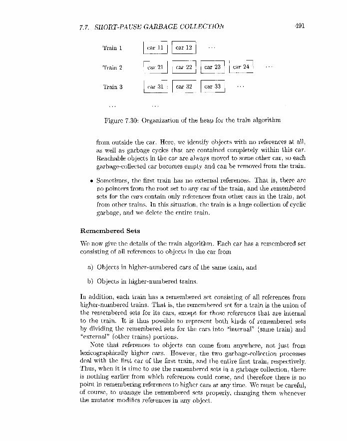
7.7. SHORT-PAUSE GARBAGE COLLECTION

Train 1

Train 2

Train 3

Figure 7.30: Organization of the heap for the train algorithm

from outside the car. Here, we identify objects with no references at all, as well as garbage cycles that are contained completely within this car. Reachable objects in the car are always moved to some other car, so each garbage-collected car becomes empty and can be removed from the train.

a Sometimes, the first train has no external references. That is, there are no pointers from the root set to any car of the train, and the remembered sets for the cars contain only references from other cars in the train, not from other trains. In this situation, the train is a huge collection of cyclic garbage, and we delete the entire train.

Remembered Sets

We now give the details of the train algorithm. Each car has a remembered set consisting of all references to objects in the car from

a) Objects in higher-numbered cars of the same train, and

b) Objects in higher-numbered trains.

In addition, each train has a remembered set consisting of all references from higher-numbered trains. That is, the remembered set for a train is the union of the remembered sets for its cars, except for those references that are internal to the train. It is thus possible to represent both kinds of remembered sets by dividing the remembered sets for the cars into "internal" (same train) and "external" (other trains) portions.

Note that references to objects can come from anywhere, not just from lexicographically higher cars. However, the two garbage-collection processes deal with the first car of the first train, and the entire first train, respectively. Thus, when it is time to use the remembered sets in a garbage collection, there is nothing earlier from which references could come, and therefore there is no point in remembering references to higher cars at any time. We must be careful, of course, to manage the remembered sets properly, changing them whenever the mutator modifies references in any object.


Managing Trains

Our objective is to draw out of the first train all objects that are not cyclic garbage. Then, the first train either becomes nothing but cyclic garbage and is therefore collected at the next round of garbage collection, or if the garbage is not cyclic, then its cars may be collected one at a time.

We therefore need to start new trains occasionally, even though there is no limit on the number of cars in one train, and we could in principle simply add new cars to a single train, every time we needed more space. For example, we could start a new train after every k object creations, for some k. That is, in general, a new object is placed in the last car of the last train, if there is room, or in a new car that is added to the end of the last train, if there is no room. However, periodically, we instead start a new train with one car, and place the new object there.

Garbage Collecting a Car

The heart of the train algorithm is how we process the first car of the first train during a round of garbage collection. Initially, the reachable set is taken to be the objects of that car with references from the root set and those with references in the remembered set for that car. We then scan these objects as in a mark-and-sweep collector, but we do not scan any reached objects outside the one car being collected. After this tracing, some objects in the car may be identified as garbage. There is no need to reclaim their space, because the entire car is going to disappear anyway.

However, there are likely to be some reachable objects in the car, and these must be moved somewhere else. The rules for moving an object are:

If there is a reference in the remembered set from any other train (which will be higher-numbered than the train of the car being collected), then move the object to one of those trains. If there is room, the object can go in some existing car of the train from which a reference emanates, or it can go in a new, last car if there is no room.

If there is no reference from other trains, but there are references from the root set or from the first train, then move the object to any other car of the same train, creating a new, last car if there is no room. If possible, pick a car from which there is a reference, to help bring cyclic structures to a single car.

After moving all the reachable objects from the first car, we delete that car.

Panic Mode

There is one problem with the rules above. In order to be sure that all garbage will eventually be collected, we need to be sure that every train eventually becomes the first train, and if this train is not cyclic garbage, then eventually

7.7. SHORT-PA USE GARBAGE COLLECTION 493

all cars of that train are removed and the train disappears one car at a time. However, by rule (2) above, collecting the first car of the first train can produce a new last car. It cannot produce two or more new cars, since surely all the objects of the first car can fit in the new, last car. However, could we be in a situation where each collection step for a train results in a new car being added, and we never get finished with this train and move on to the other trains?

The answer is, unfortunately, that such a situation is possible. The problem arises if we have a large, cyclic, nongarbage structure, and the mutator manages to change references in such a way that we never see, at the time we collect a car, any references from higher trains in the remembered set. If even one object is removed from the train during the collection of a car, then we are OK, since no new objects are added to the first train, and therefore the first train will surely run out of objects eventually. However, there may be no garbage at all that we can collect at a stage, and we run the risk of a loop where we perpetually garbage collect only the current first train.

To avoid this problem, we need to behave differently whenever we encounter a futile garbage collection, that is, a car from which not even one object can be deleted as garbage or moved to another train. In this "panic mode," we make two changes:

1. When a reference to an object in the first train is rewritten, we maintain the reference as a new member of the root set.

2. When garbage collecting, if an object in the first car has a reference from the root set, including dummy references set up by point (I), then we move that object to another train, even if it has no references from other trains. It is not important which train we move it to, as long as it is not the first train.

In this way, if there are any references from outside the first train to objects in the first train, these references are considered as we collect every car, and eventually some object will be removed from that train. We can then leave panic mode and proceed normally, sure that the current first train is now smaller than it was.


Exercise 7.7.1 : Suppose that the network of objects from Fig. 7.20 is managed by an incremental algorithm that uses the four lists Unreached, Unscanned, Scanned, and Free, as in Baker's algorithm. To be specific, the Unscanned list is managed as a queue, and when more than one object is to be placed on this list due to the scanning of one object, we do so in alphabetical order. Suppose also that we use write barriers to assure that no reachable object is made garbage. Starting with A and B on the Unscanned list, suppose the following events occur:

i . A is scanned.


ii. The pointer A -+ D is rewritten to be A -+ H.

iii. B is scanned.

iv. D is scanned.

v. The pointer B -+ C is rewritten to be B -+ I.

Simulate the entire incremental garbage collection, assuming no more pointers are rewritten. Which objects are garbage? Which objects are placed on the Free list?

Exercise 7.7.2 : Repeat Exercise 7.7.1 on the assumption that

a) Events (ii) and (v) are interchanged in order.

b) Events (ii) and (v) occur before (i), (iii), and (iv).

Exercise 7.7.3 : Suppose the heap consists of exactly the nine cars on three trains shown in Fig. 7.30 (i.e., ignore the ellipses). Object o in car I1 has references from cars 12, 23, and 32. When we garbage collect car 11, where might o wind up?

Exercise 7.7.4 : Repeat Exercise 7.7.3 for the cases that o has

a) Only references from cars 22 and 31.

b) No references other than from car 11.

Exercise 7.7.5 : Suppose the heap consists of exactly the nine cars on three trains shown in Fig. 7.30 (i.e., ignore the ellipses). We are currently in panic mode. Object 01 in car 11 has only one reference, from object 02 in car 12. That reference is rewritten. When we garbage collect car 11, what could happen to ol?

7.8 Advanced Topics in Garbage Collection We close our investigation of garbage collection with brief treatments of four additional topics:

1. Garbage collection in parallel environments.

2. Partial relocations of objects.

3. Garbage collection for languages that are not type-safe.

4. The interaction between programmer-controlled and automatic garbage collect ion.

7.8. ADVANCED TOPICS IN GARBAGE COLLECTION

7.8.1 Parallel and Concurrent Garbage Collection

Garbage collection becomes even more challenging when applied to applications running in parallel on a multiprocessor machine. It is not uncommon for server applications to have thousands of threads running at the same time; each of these threads is a mutator. Typically, the heap will consist of gigabytes of memory.

Scalable garbage-collection algorithms must take advantage of the presence of multiple processors. We say a garbage collector is parallel if it uses multiple threads; it is concurrent if it runs simultaneously with the mutator.

We shall describe a parallel, and mostly concurrent, collector that uses a concurrent and parallel phase that does most of the tracing work, and then a stop-the-world phase that guarantees all the reachable objects are found and reclaims the storage. This algorithm introduces no new basic concepts in garbage collection per se; it shows how we can combine the ideas described so far to create a full solution to the parallel-and-concurrent collection problem. How- ever, there are some new implementation issues that arise due to the nature of parallel execution. We shall discuss how this algorithm coordinates multiple threads in a parallel computation using a rather common work-queue model.

To understand the design of the algorithm we must keep in mind the scale of the problem. Even the root set of a parallel application is much larger, consisting of every thread's stack, register set and globally accessible variables. The amount of heap storage can be very large, and so is the amount of reachable data. The rate at which mutations take place is also much greater.

To reduce the pause time, we can adapt the basic ideas developed for incremental analysis to overlap garbage collection with mutation. Recall that an incremental analysis, as discussed in Section 7.7, performs the following three steps:

1. Find the root set. This step is normally performed atomically, that is, with the mutator(s) stopped.

Interleave the tracing of the reachable objects with the execution of the mutator(s). In this period, every time a mutator writes a reference that points from a Scanned object to an Unreached object, we remember that reference. As discussed in Section 7.7.2, we have options regarding the granularity with which these references are remembered. In this section, we shall assume the card-based scheme, where we divide the heap into sections called "cards" and maintain a bit map indicating which cards are dir ty (have had one or more references within them rewritten).

3. Stop the mutator(s) again to rescan all the cards that may hold references to unreached objects.

For a large multithreaded application, the set of objects reached by the root set can be very large. It is infeasible to take the time and space to visit all such objects while all mutations cease. Also, due to the large heap and the large


number of mutation threads, many cards may need to be rescanned after all objects have been scanned once. It is thus advisable to scan some of these cards in parallel, while the mutators are allowed to continue to execute concurrently.

To implement the tracing of step (2) above, in parallel, we shall use multiple garbage-collecting threads concurrently with the mutator threads to trace most of the reachable objects. Then, to implement step (3), we stop the mutators and use parallel threads to ensure that all reachable objects are found.

The tracing of step (2) is carried out by having each mutator thread perform part of the garbage collection, along with its own work. In addition, we use threads that are dedicated purely to collecting garbage. Once garbage collection has been initiated, whenever a mutator thread performs some memory- allocation operation, it also performs some tracing computation. The pure garbage-collecting threads are put to use only when a machine has idle cycles. As in incremental analysis, whenever a mutator writes a reference that points from a Scanned object to an Unreached object, the card that holds this reference is marked dirty and needs to be rescanned.

Here is an outline of the parallel, concurrent garbage-collection algorithm.

1. Scan the root set for each mutator thread, and put all objects directly reachable from that thread into the Unscanned state. The simplest incremental approach to this step is to wait until a mutator thread calls the memory manager, and have it scan its own root set if that has not already been done. If some mutator thread has not called a memory allocation function, but all the rest of tracing is done, then this thread must be interrupted to have its root set scanned.

2. Scan objects that are in the Unscanned state. To support parallel computation, we use a work queue of fixed-size work packets, each of which holds a number of Unscanned objects. Unscanned objects are placed in work packets as they are discovered. Threads looking for work will de- queue these work packets and trace the Unscanned objects therein. This strategy allows the work to be spread evenly among workers in the tracing process. If the system runs out of space, and we cannot find the space to create these work packets, we simply mark the cards holding the objects to force them to be scanned. The latter is always possible because the bit array holding the marks for the cards has already been allocated.

3. Scan the objects in dirty cards. When there are no more Unscanned objects left in the work queue, and all threads' root sets have been scanned, the cards are rescanned for reachable objects. As long as the mutators continue to execute, dirty cards continue to be produced. Thus, we need to stop the tracing process using some criterion, such as allowing cards to be rescanned only once or a fixed number of times, or when the number of outstanding cards is reduced to some threshold. As a result, this parallel and concurrent step normally terminates before completing the trace, which is finished by the final step, below.

7.8. ADVANCED TOPICS IN GARBAGE COLLECTION

4. The final step guarantees that all reachable objects are marked as reached. With all the mutators stopped, the root sets for all the threads can now be found quickly using all the processors in the system. Because the reachability of most objects has been traced, only a small number of objects are expected to be placed in the Unscanned state. All the threads then participate in tracing the rest of the reachable objects and rescanning all the cards.

It is important that we control the rate at which tracing takes place. The tracing phase is like a race. The mutators create new objects and new references that must be scanned, and the tracing tries to scan all the reachable objects and rescan the dirty cards generated in the meanwhile. It is not desirable to start the tracing too much before a garbage collection is needed, because that will increase the amount of floating garbage. On the other hand, we cannot wait until the memory is exhausted before the tracing starts, because then mutators will not be able to make forward progress and the situation degenerates to that of a stop-the-world collector. Thus, the algorithm must choose the time to commence the collection and the rate of tracing appropriately. An estimate of the mutation rate from previous cycles of collection can be used to help in the decision. The tracing rate is dynamically adjusted to account for the work performed by the pure garbage-collecting threads.

7.8.2 Partial Object Relocation

As discussed starting in Section 7.6.4, copying or compacting collectors are advantageous because they eliminate fragmentation. However, these collectors have nontrivial overheads. A compacting collector requires moving all objects and updating all the references at the end of garbage collection. A copying collector figures out where the reachable objects go as tracing proceeds; if tracing is performed incrementally, we need either to translate a mutator's every reference, or to move all the objects and update their references at the end. Both options are very expensive, especially for a large heap.

We can instead use a copying generational garbage collector. It is effective in collecting immature objects and reducing fragmentation, but can be expensive when collecting mature objects. We can use the train algorithm to limit the amount of mature data analyzed each time. However, the overhead of the train algorithm is sensitive to the size of the remembered set for each partition.

There is a hybrid collection scheme that uses concurrent tracing to reclaim all the unreachable objects and at the same time moves only a part of the objects. This method reduces fragmentation without incurring the full cost of relocation in each collection cycle.

1. Before tracing begins, choose a part of the heap that will be evacuated.

2. As the reachable objects are marked, also remember all the references pointing to objects in the designated area.


3. When tracing is complete, sweep the storage in parallel to reclaim the space occupied by unreachable objects.

4. Finally, evacuate the reachable objects occupying the designated area and fix up the references to the evacuated objects.

7.8.3 Conservative Collection for Unsafe Languages

As discussed in Section 7.5.1, it is impossible to build a garbage collector that is guaranteed to work for all C and C++ programs. Since we can always compute an address with arithmetic operations, no memory locations in C and C++ can ever be shown to be unreachable. However, many C or C++ programs never fabricate addresses in this way. It has been demonstrated that a conservative garbage collector - one that does not necessarily discard all garbage - can be built to work well in practice for this class of programs.

A conservative garbage collector assumes that we cannot fabricate an address, or derive the address of an allocated chunk of memory without an address pointing somewhere in the same chunk. We can find all the garbage in programs satisfying such an assumption by treating as a valid address any bit pattern found anywhere in reachable memory, as long as that bit pattern may be construed as a memory location. This scheme may classify some data erro- neously as addresses. It is correct, however, since it only causes the collector to be conservative and keep more data than necessary.

Object relocation, requiring all references to the old locations be updated to point to the new locations, is incompatible with conservative garbage collection. Since a conservative garbage collector does not know if a particular bit pattern refers to an actual address, it cannot change these patterns to point to new addresses.

Here is how a conservative garbage collector works. First, the memory manager is modified to keep a data map of all the allocated chunks of memory. This map allows us to find easily the starting and ending boundary of the chunk of memory that spans a certain address. The tracing starts by scanning the program's root set to find any bit pattern that looks like a memory location, without worrying about its type. By looking up these potential addresses in the data map, we can find the starting addresses of those chunks of memory that might be reached, and place them in the Unscanned state. We then scan all the unscanned chunks, find more (presumably) reachable chunks of memory, and place them on the work list until the work list becomes empty. After tracing is done, we sweep through the heap storage using the data map to locate and free all the unreachable chunks of memory.

7.8.4 Weak References

Sometimes, programmers use a language with garbage collection, but also wish to manage memory, or parts of memory, themselves. That is, a programmer may know that certain objects are never going to be accessed again, even though

7.8. ADVANCED TOPICS IN GARBAGE COLLECTION 499

references t o the objects remain. An example from compiling will suggest the problem.

Example 7.17 : We have seen that the lexical analyzer often manages a symbol table by creating an object for each identifier it sees. These objects may appear as lexical values attached to leaves of the parse tree representing those identifiers, for instance. However, it is also useful to create a hash table, keyed by the identifier's string, to locate these objects. That table makes it easier for the lexical analyzer to find the object when it encounters a lexeme that is an identifier.

When the compiler passes the scope of an identifier I, its symbol-table object no longer has any references from the parse tree, or probably any other intermediate structure used by the compiler. However, a reference to the object is still sitting in the hash table. Since the hash table is part of the root set of the compiler, the object cannot be garbage collected. If another identifier with the same lexeme as I is encountered, then it will be discovered that I is out of scope, and the reference to its object will be deleted. However, if no other identifier with this lexeme is encountered, then I 's object may remain as uncollectable, yet useless, throughout compilation. O

If the problem suggested by Example 7.17 is important, then the compiler writer could arrange to delete from the hash table all references to objects as soon as their scope ends. However, a technique known as weak references allows the programmer to rely on automatic garbage collection, and yet not have the heap burdened with reachable, yet truly unused, objects. Such a system allows certain references to be declared "weak." An example would be all the references in the hash table we have been discussing. When the garbage collector scans an object, it does not follow weak references within that object, and does not make the objects they point t o reachable. Of course, such an object may still be reachable if there is another reference to it that is not weak.


! Exercise 7.8.1 : In Section 7.8.3 we suggested that it was possible to garbage collect for C programs that do not fabricate expressions that point to a place within a chunk unless there is an address that points somewhere within that same chunk. Thus, we rule out code like

because, while p might point to some chunk accidentally, there could be no other pointer to that chunk. On the other hand, with the code above, it is more likely that p points nowhere, and executing that code will result in a segmentation fault. However, in C it is possible to write code such that a variable like p is guaranteed to point to some chunk, and yet there is no pointer to that chunk. Write such a program.


7.9 Summary of Chapter 7

+ Run-Time Organixation. To implement the abstractions embodied in the source language, a compiler creates and manages a run-time environment in concert with the operating system and the target machine. The run- time environment has static data areas for the object code and the static data objects created at compile time. It also has dynamic stack and heap areas for managing objects created and destroyed as the target program executes.

+ Control Stack. Procedure calls and returns are usually managed by a run- time stack called the control stack. We can use a stack because procedure calls or activations nest in time; that is, if p calls q, then this activation of q is nested within this activation of p.

+ Stack Allocation. Storage for local variables can allocated on a run-time stack for languages that allow or require local variables to become inaccessible when their procedures end. For such languages, each live activation has an activation record (or frame) on the control stack, with the root of the activation tree at the bottom, and the entire sequence of activation records on the stack corresponding to the path in the activation tree to the activation where control currently resides. The latter activation has its record at the top of the stack.

+ Access t o Nonlocal Data on the Stack. For languages like C that do not allow nested procedure declarations, the location for a variable is either global or found in the activation record on top of the run-time stack. For languages with nested procedures, we can access nonlocal data on the stack through access links, which are pointers added to each activation record. The desired nonlocal data is found by following a chain of access links to the appropriate activation record. A display is an auxiliary array, used in conjunction with access links, that provides an efficient short-cut alternative to a chain of access links.

+ Heap Management. The heap is the portion of the store that is used for data that can live indefinitely, or until the program deletes it explicitly. The memory manager allocates and deallocates space within the heap. Garbage collection finds spaces within the heap that are no longer in use and can therefore be reallocated to house other data items. For languages that require it, the garbage collector is an important subsystem of the memory manager.

+ Exploiting Locality. By making good use of the memory hierarchy, memory managers can influence the run time of a program. The time taken to access different parts of memory can vary from nanoseconds to milliseconds. Fortunately, most programs spend most of their time executing a relatively small fraction of the code and touching only a small fraction of

7.9. SUMMARY OF CHAPTER 7

the data. A program has temporal locality if it is likely to access the same memory locations again soon; it has spatial locality if it is likely to access nearby memory locations soon.

+ Reducing Fragmentation. As the program allocates and deallocates memory, the heap may get fragmented, or broken into large numbers of small noncontiguous free spaces or holes. The best fit strategy - allocate the smallest available hole that satisfies a request - has been found empirically to work well. While best fit tends to improve space utilization, it may not be best for spatial locality. Fragmentation can be reduced by combining or coalescing adjacent holes.

+ Manual Deallocation. Manual memory management has two common failings: not deleting data that can not be referenced is a memory-leak error, and referencing deleted data is a dangling-pointer-dereference error.

+ Reachability. Garbage is data that cannot be referenced or reached. There are two basic ways of finding unreachable objects: either catch the transition as a reachable object turns unreachable, or periodically locate all reachable objects and infer that all remaining objects are unreachable.

+ Reference-Counting Collectors maintain a count of the references to an object; when the count transitions to zero, the object becomes unreachable. Such collectors introduce the overhead of maintaining references and can fail to find "cyclic" garbage, which consists of unreachable objects that reference each other, perhaps through a chain of references.

+ Trace- Based Garbage Collectors iteratively examine or trace all references to find reachable objects, starting with the root set consisting of objects that can be accessed directly without having to dereference any pointers.

+ Mark-and-Sweep Collectors visit and mark all reachable objects in a first tracing step and then sweep the heap to free up unreachable objects.

+ Mark-and-Compact Collectors improve upon mark-and-sweep; they relocate reachable objects in the heap to eliminate memory fragmentation.

+ Copying Collectors break the dependency between tracing and finding free space. They partition the memory into two semispaces, A and B. Allocation requests are satisfied from one semispace, say A, until it fills up, a t which point the garbage collector takes over, copies the reachable objects to the other space, say B, and reverses the roles of the semispaces.

+ Incremental Collectors. Simple trace-based collectors stop the user program while garbage is collected. Incremental collectors interleave the actions of the garbage collector and the mutator or user program. The mutator can interfere with incremental reachability analysis, since it can


change the references within previously scanned objects. Incremental collectors therefore play it safe by overestimating the set of reachable objects; any "floating garbage" can be picked up in the next round of collection.

+ Partial Collectors also reduce pauses; they collect a subset of the garbage at a time. The best known of partial-collection algorithms, generational garbage collection, partitions objects according to how long they have been allocated and collects the newly created objects more often because they tend to have shorter lifetimes. An alternative algorithm, the train algorithm, uses fixed length partitions, called cars, that are collected into trains. Each collection step is applied to the first remaining car of the first remaining train. When a car is collected, reachable objects are moved out to other cars, so this car is left with garbage and can be removed from the train. These two algorithms can be used together to create a partial collector that applies the generational algorithm to younger objects and the train algorithm to more mature objects.

7.10 References for Chapter 7

In mathematical logic, scope rules and parameter passing by substitution date back to Frege [8]. Church's lambda calculus [3] uses lexical scope; it has been used as a model for studying programming languages. Algol 60 and its successors, including C and Java, use lexical scope. Once introduced by the initial implementation of Lisp, dynamic scope became a feature of the language; Mc- Carthy [14] gives the history.

Many of the concepts related to stack allocation were stimulated by blocks and recursion in Algol 60. The idea of a display for accessing nonlocals in a lexically scoped language is due to Dijkstra [5]. A detailed description of stack allocation, the use of a display, and dynamic allocation of arrays appears in Randell and Russell [16]. Johnson and Ritchie [lo] discuss the design of a calling sequence that allows the number of arguments of a procedure to vary from call to call.

Garbage collection has been an active area of investigation; see for example Wilson [17]. Reference counting dates back to Collins [4]. Trace-based collection dates back to McCarthy [13], who describes a mark-sweep algorithm for fixed- length cells. The boundary-tag for managing free space was designed by Knuth in 1962 and published in [ll].

Algorithm 7.14 is based on Baker [I]. Algorithm 7.16 is based on Cheney's [2] nonrecursive version of Fenichel and Yochelson's [7] copying collector.

Incremental reachability analysis is explored by Dijkstra et al. [6]. Lieber- man and Hewitt [12] present a generational collector as an extension of copying collection. The train algorithm began with Hudson and Moss [9].

I . Baker, H. G. Jr., "The treadmill: real-time garbage collection without motion sickness," ACM SIGPLAN Notices 27:3 (Mar., 1992), pp. 66-70.

7.10. REFERENCES FOR CHAPTER 7 503

2. Cheney, C. J . , "A nonrecursive list compacting algorithm," Comm. ACM 13:ll (Nov., 1970), pp. 677-678.

3. Church, A., The Calculi of Lambda Conversion, Annals of Math. Studies, No. 6, Princeton University Press, Princeton, N. J. , 1941.

4. Collins, G. E., "A method for overlapping and erasure of lists," Comm. ACM 2:12 (Dec., 1960), pp. 655-657.

5. Dijkstra, E. W ., "Recursive programming," Numerische Math. 2 (1960), pp. 312-318.

6. Dijkstra, E. W., L. Lamport, A. J. Martin, C. S. Scholten, and E. F. M. Steffens, "On-the-fly garbage collection: an exercise in cooperation," Comm. ACM 21: l l (1978), pp. 966-975.

7. Fenichel, R. R. and J . C. Yochelson, "A Lisp garbage-collector for virtual- memory computer systems", Comm. ACM 12:11 (1969), pp. 611-612.

8. Frege, G., "Begriffsschrift, a formula language, modeled upon that of arithmetic, for pure thought," (1879). In J . van Heijenoort, From Frege to Godel, Harvard Univ. Press, Cambridge MA, 1967.

9. Hudson, R. L. and J . E. B. Moss, "Incremental Collection of Mature Objects", Proc. Intl. Workshop on Memory Management, Lecture Notes In Computer Science 637 (1992), pp. 388-403.

10. Johnson, S. C. and D. M. Ritchie, "The C language calling sequence," Computing Science Technical Report 102, Bell Laboratories, Murray Hill NJ, 1981.

11. Knuth, D. E., Art of Computer Programming, Volume I : Fundamental Algorithms, Addison-Wesley, Boston MA, 1968.

12. Lieberman, H. and C. Hewitt, "A real-time garbage collector based on the lifetimes of objects," Comm. ACM 26:6 (June 1983), pp. 419-429.

13. McCarthy, J. , "Recursive functions of symbolic expressions and their computation by machine," Comm. ACM 3:4 (Apr., 1960), pp. 184-195.

14. McCarthy, J . , L'History of Lisp." See pp. 173-185 in R. L. Wexelblat (ed.), History of Programming Languages, Academic Press, New York, 1981.

15. Minsky, M., "A LISP garbage collector algorithm using secondary storage," A. I. Memo 58, MIT Project MAC, Cambridge MA, 1963.

16. Randell, B. and L. J. Russell, Algol 60 Implementation, Academic Press, New York, 1964.

17. Wilson, P. R., "Uniprocessor garbage collection techniques,"

run-time environments - information sciences...

Documents