Securitized Banking and the Run on Repo

Gary Gorton Yale and NBER

Andrew Metrick Yale and NBER

First version: January 22, 2009 This version: November 13, 2009

Abstract The Panic of 2007-2008 was a run on the sale and repurchase market (the “repo” market), which is a very large, short-term market that provides financing for a wide range of securitization activities and financial institutions. Repo transactions are collateralized, frequently with securitized bonds. We refer to the combination of securitization plus repo finance as “securitized banking”, and argue that these activities were at the nexus of the crisis. We use a novel data set that includes credit spreads for hundreds of securitized bonds to trace the path of crisis from subprime-housing related assets into markets that had no connection to housing. We find that changes in the “LIB-OIS” spread, a proxy for counterparty risk, was strongly correlated with changes in credit spreads and repo rates for securitized bonds. These changes implied higher uncertainty about bank solvency and lower values for repo collateral. Concerns about the liquidity of markets for the bonds used as collateral led to increases in repo “haircuts”: the amount of collateral required for any given transaction. With declining asset values and increasing haircuts, the U.S. banking system was effectively insolvent for the first time since the Great Depression. *We thank Lei Xie for research assistance, Sara Paolella for editorial assistance, numerous anonymous traders for help with data, and seminar participants at the NY Federal Reserve Bank, the Board of Governors of the Federal Reserve System, Texas, MIT, and Harvard for comments.

  1

The current financial crisis is a system-wide bank run. What makes this bank run special is

that it did not occur in the traditional-banking system, but instead took place in the “securitized-

banking” system. A traditional-banking run is driven by the withdrawal of deposits, while a

securitized-banking run is driven by the withdrawal of repurchase (“repo”) agreements. Hence,

we describe the crisis as a “run on repo”. The purpose of this paper is to propose a mechanism

for this new kind of bank run, and to provide supporting evidence for this mechanism through

analysis of a novel data set.

Traditional banking is the business of making and holding loans, with insured demand

deposits as the main source of funds. Securitized banking is the business of packaging and

reselling loans, with repo agreements as the main source of funds. Securitized-banking activities

were central to the operations of firms formerly known as “investment banks” (e.g. Bear Stearns,

Lehman Brothers, Morgan Stanley, Merrill Lynch), but they also play a role at commercial

banks, as a supplement to traditional-banking activities of firms like Citigroup, J.P. Morgan, and

Bank of America.1

We argue that the financial crisis that began in August 2007 is a “systemic event,” defined in

this paper to mean that the banking sector became insolvent. What happened is analogous to the

banking panics of the 19th century in which depositors en masse went to their banks seeking to

withdraw cash in exchange of demand and savings deposits. The banking system could not

honor these demands because the cash had been lent out and the loans were illiquid, so instead

they suspended convertibility and relied on clearinghouses to issue certificates as makeshift

currency.2 Evidence of the insolvency of the banking system in these earlier episodes is the

discount on these certificates. We argue that the current crisis is similar in that contagion led to

“withdrawals” in the form of unprecedented high repo haircuts and even the cessation of repo

lending on many forms of collateral. Evidence of insolvency in 2008 is the bankruptcy or forced

                                                        1 We have chosen a new term, “securitized banking”, to emphasize the role of the securitization process both as the main intermediation activity and as a crucial source of the collateral used to raise funds in repo transactions. Other banking terms – “wholesale banking”, “shadow banking,” or “investment banking” – have broader connotations and do not completely encompass our definition of securitized banking. The closest notion to our definition of securitized banking is the model of “unstable banking” proposed by Shleifer and Vishny (2009). 2 The clearinghouse private money was a claim on the coalition of banks, rather than a liability of any individual bank. By broadening the backing for the claim, the clearinghouse made the claim safer, a kind of insurance. Gorton (1985) and Gorton and Mullineaux (1987) discuss the clearinghouse response to panics. Also, see Gorton and Huang (2006).

  2

rescue of several large firms, with other (even larger) firms requiring government support to stay

in business.

To perform our analysis, we use a novel data set with information on 392 securitized bonds

and related assets, including many classes of asset-backed securities (ABS), collateralized-debt

obligations (CDOs), credit-default swaps (CDS), repo rates, and repo haircuts.3 Using these

data, we are able to provide a new perspective on the contagion in this crisis. In our exposition,

we use this term “contagion” specifically to mean the spread of the crisis from subprime-housing

assets to non-subprime assets that have no direct connection to the housing market.

To provide background for our analysis, we illustrate the differences between traditional

banking and securitized banking in Figures 1 and 2. Figure 1 provides the classic picture of the

financial intermediation of mortgages by the traditional-banking system. In Step A, depositors

transfer money to the bank, in return for a checking or savings account that can be withdrawn at

any time. In Step B, the bank loans these funds to a borrower, who promises to repay through a

mortgage on the property. The bank then holds this mortgage on its balance sheet, along with

other non-mortgage loans made to retail and commercial borrowers.

Traditional-banking runs were ended in United States in the 1930s with the introduction of

deposit insurance and discount-window lending by the Federal Reserve. With deposits insured

by the federal government, depositors have little incentive to withdraw their funds. Deposit

insurance works well for retail investors, but still leaves a challenge for large institutions. When

deposit insurance was capped at $100,000, institutions such as sovereign-wealth funds, mutual

funds, and cash-rich companies did not have easy access to safe short-term investments. One

solution to this problem is the securitized-banking system illustrated in Figure 2, which takes

large “deposits” from investors (Step 1), and then intermediates these deposits to mortgage

borrowers (Steps 2 and 3) and other debtors.

Step 1 in Figure 2 is an analogue to Step A from Figure 1, but there is one important

difference. In the traditional-banking system shown in Figure 1, the deposits are insured by the

government. To achieve similar protection in Step 1 of Figure 2, the investor receives collateral

from the bank. In practice, this deposit-collateral transaction takes the form of a repo agreement:

the investor buys some asset (=collateral) from the bank for $X, and the bank agrees to

                                                        3 This paper uses many terms and abbreviations that are atypical or new to the academic literature. Beginning in Section I, the first appearance of these terms is given in bold type, and definitions of bolded terms are given in Appendix A.

  3

repurchase the same asset some time later (perhaps the next day) for $Y. The percentage (Y-

X)/X is the “repo rate”, and is analogous to the interest rate on a bank deposit. Typically, the

total amount of the deposit will be some amount less than the value of the underlying asset, with

the difference called a “haircut”. For example, if an asset has a market value of $100 and a bank

sells it for $80 with an agreement to repurchase it for $88, then we would say that the repo rate is

10 percent (= 88-80 / 80), and the haircut is 20 percent (100 – 80 / 100). If the bank defaults on

the promise to repurchase, then the investor keeps the collateral.

Turning next to the lower right corner of Figure 2, we show how the second part of the

intermediation differs from traditional banking. In Figure 1, the bank did the work of

underwriting the loan itself. In Figure 2, the bank outsources this function to a direct lender.

Such lenders grew to prominence in the most recent housing boom, with a specialization of

underwriting loans to be held for only a short time before being sold to banks. Much has been

written about potential conflicts in this separation of the loan decision from the source of finance,

but that is not our topic here. In principle, there is no reason that this separation must necessarily

lead to poor underwriting, and in any event such problems do not imply anything about

contagion or systemic events.

Another key component of securitized banking is in the “securitization” itself: the

intermediation activities that transfer most of the mortgage loans to outside investors in Step 4.

We will discuss this step in detail in Section I of the paper. For our purposes here, the key idea is

that the outputs of this securitization are often used as collateral in Step 1, so that securitized

banking is a cycle that requires all steps to keep running. In this paper, we will show how this

cycle broke down in the crisis.

Figure 3 summarizes the relationships between the main elements of traditional and

securitized banking. The left column lists the familiar elements of traditional banking: reserves,

deposit insurance, interest rates on deposits, and the holding of loans on balance sheet. Bank

solvency is promoted by requiring a fraction of deposits to be held in reserve, and in emergencies

these reserves can be replenished by borrowing from the central bank. The analogue in

securitized banking is the repo haircut, which forces banks to keep some fraction of their assets

in reserve when they borrow money through repo markets. The next row, deposit insurance, is a

promise made by the government to pay depositors in the event of default. The analogue in

securitized banking is collateral. Next, a bank in need of cash can raise deposit rates to attract it;

  4

the analogues for securitized banking are the repo rates. Finally, the cash raised in traditional

banking is lent out, with the resulting loans held on the balance sheet. In securitized banking,

funds are lent only temporarily, with loans repackaged and resold as securitized bonds. Some of

these bonds are also used as collateral to raise more funds, which completes the cycle.

The “run on repo” can be seen in Figure 4, which plots a “haircut index” from 2007 to 2008.

The details of this index will be explained below in Section III; for now, just think of the index

as an average haircut for collateral used in repo transactions, not including U.S. treasury

securities. This index rises from zero in early 2007 to nearly 50 percent at the peak of the crisis

in late 2008. During this time period, several classes of assets stopped entirely from being used

as collateral, an unprecedented event that is equivalent to a haircut of 100 percent.

To see how the increase in haircuts can drive the banking system to insolvency, take as a

benchmark a repo market size of, for example, $10 trillion. With zero haircuts, this is the amount

of financing that banks can achieve in the repo markets. When the weighted-average haircut

reaches, say, 20 percent, then banks have a shortage of $2 trillion. In the crisis, some of this

amount was raised early on by issuing new securities. But, this fell far short of what was needed.

Furthermore, selling the underlying collateral drives asset prices down, which then reinforces the

cycle: lower prices, less collateral, more concerns about solvency, and ever increasing haircuts.

We focus on the repo market because of its size (discussed below). But, there were also

other important runs, in particular, on asset-backed commercial paper programs and structured

investment vehicles. Papers that document the runs on asset-backed commercial paper programs

during the crisis include Covitz,  Liang,  and  Suarez  (2009)  and  Carey,  Correa,  and  Kotter 

(2009).    Also,  important  was  the  run  on  money  market  funds  following  the  failure  of 

Lehman Brothers.  See the Investment Company Institute (2009).

This paper and those mentioned above, are part of a rapidly growing literature that tries to

empirically document what happened during the crisis. Aside from runs the financial crisis is

complicated in many other dimensions as well. There are studies of the breakdown of various 

arbitrage relationships, perhaps due to counterparty risk and attendant funding problems, 

e.g., Coffey, Hrung, and Sarkar (2009), Gorton (2009), Baba and Packer (2009), Stanton and 

Wallace (2009), Fontana (2009), and Fender and Scheicher (2009).  Other research looks at 

counterparty risk and liquidity, e.g., Arora, Gandhi, and Longstaff (2009), Schwarz (2009), 

and  Singh  and  Aitken  (2009).    There  are  also  papers  that  document  the  international 

  5

dimensions of the crisis, and compare the crisis to previous crises, e.g., Eichengreen, Mody, 

Nedeljkovic, and Sarno (2009) and Reinhart and Rogoff (2008).   Ivashina and Scharfstein 

(2008)  look  at  bank  lending  during  the  crisis.    The  real  effects  of  the  crisis  are  also 

important  to  document,  e.g.,  Almeida,  Campello,  and  Laranjeira  (2009)  or  Campello, 

Giabona,  Graham,  and  Harvey  (2009).    Many  other  papers  look  at  subprime mortgages, 

rating agencies, auction rate securities, short selling prohibitions, and so on, so the above 

list is very far from being complete.4

The remainder of the paper is organized as follows. In Section I, we provide institutional

background for our analysis, with a discussion of the growth of securitized banking, using

subprime mortgages as the case study. We use this case study to provide more detail for Step 4

in Figure 2, and to explain the mechanics of securitization and the repo market.

In Section II, we introduce and explain the two main state variables used in the paper: the

ABX index – which proxies for fundamentals in the subprime mortgage market – and the LIB-

OIS, which is the spread between the LIBOR rate (for unsecured interbank borrowing) and the

rate on an overnight interest swap, OIS (a proxy for the risk-free rate). The LIB-OIS can be

thought of as a proxy for counterparty risk in repo transactions. We then plot these state

variables for 2007 and 2008 and review the timeline for the crisis. The ABX data show that the

deterioration of the subprime market began in early 2007. As is now well known, this

deterioration had a direct impact on banks, which had many of these securitized assets and pre-

securitized mortgages on their balance sheets. This real deterioration in bank balance sheets

became apparent in the interbank markets in mid-2007, as evidenced by an upward spike in the

LIB-OIS in August. This state variable remained in a historically high but narrow range until

September 2008, when the events at Fannie Mae, Freddie Mac, Lehman, and AIG led to a rapid

deterioration in interbank markets and increase in the LIB-OIS that persisted until the end of

2008.

We posit that the increased risk at banks had several interrelated effects, all of which

centered on the securitized assets used as collateral in the repo market. We provide evidence for

these effects, using a data set with information on securitized bonds, credit-default swaps, and

other assets used in repo transactions. These data are created by large financial institutions and                                                         4 There is also a growing theory literature. Some examples are Acharya, Gale, and Yorulmazer (2009), Brunnermeier and Pedersen (2009), Geanakoplos (2009), Dang, Gorton and Holmström (2009), He and Xiong (2009), Pagano and Volpin (2009), and Shleifer and Vishny (2009).

  6

are used for trading and portfolio valuation by a wide range of market participants. Section III

provides summary statistics on these data and illustrates how some of these assets co-moved with

the ABX and the LIB-OIS.

Section IV gives the main empirical results of the paper. Without a structural model of repo

markets, we are only able to talk about co-movement of spreads on various assets, and thus we

use the language of “correlation” rather than “causation” in our empirical analysis. Section IV.A

explains our methodology and presents results for a few representative asset classes. Section

IV.B uses the full set of asset classes to demonstrate that it was the interbank markets (LIB-OIS),

and not the subprime housing market (ABX), that was correlated with increases in the spreads on

non-subprime securitized assets and related derivatives. These increased spreads are equivalent

to a price decrease, which represents a fall in the value of collateral used in repo transactions.

Then, as lenders began to fear for the stability of the banks and the possibility that they might

need to seize and sell collateral, the borrowers were forced to raise repo rates and haircuts. Both

of these increases occurred in the crisis. In Section IV.C, we find that these increases were

correlated with changes in the LIB-OIS (for repo rates) and changes in the volatility of the

underlying collateral (for repo haircuts). It is the rise in haircuts that constitutes the run on repo.

Section V reviews our arguments and concludes the paper. Appendix A defines some of the

paper’s terminology that may be unfamiliar for some readers, and also includes descriptions for

each of the asset classes of securitized bonds that are used in our empirical analysis. Appendix B

gives more detail on the data construction.

I. Institutional Background

This section discusses the main institutional features that intersected in the crisis: the

subprime mortgage market (Section I.A), securitization (Section I.B), and repo finance (Section

I.C).

A. The Subprime Mortgage Market

Home ownership for all Americans has been a long-standing national goal. This goal was

behind the origins of modern housing finance during the Great Depression with the New Deal’s

National Housing Act of 1934 (see, e.g., Fishback, Horrace and Kantor (2001)). For example, as

President Bush put it in 2004: “Not enough minorities own their own homes. … One thing I’ve

  7

done is I’ve called on private sector mortgage banks and banks to be more aggressive about

lending to first-time home buyers.” 5 The private sector responded.

The subprime mortgage market is a financial innovation, aimed at providing housing finance

to (disproportionately poor and minority) people with some combination of spotty credit

histories, a lack of income documentation, or no money for a down payment. Historically, this

group was perceived by banks as too risky to qualify for the usual mortgage products, for

example, a 30-year fixed rate mortgage. As explained by Gorton (2008), the innovation was to

structure the mortgage to effectively make the maturity two or three years. This was

accomplished with a fixed initial-period interest rate, but then at the “reset date” having the rate

rise significantly, essentially requiring the borrower to refinance the mortgage. With rising home

prices, borrowers would build equity in their homes and would be able to refinance.

The innovation was a success, if measured in terms of originations. In the years 2001-2006, a

total of about $2.5 trillion of subprime mortgages were originated.6 Almost half of this total

came in 2005 and 2006, a large portion of which was likely refinancings of previous mortgages.

B. Securitization

An important part of the subprime mortgage innovation was how the mortgages were

financed. In 2005 and 2006, about 80 percent of the subprime mortgages were financed via

securitization, that is, the mortgages were sold in residential mortgage-backed securities

(RMBS), which involves pooling thousands of mortgages together, selling the pool to a special

purpose vehicle (SPV) which finances their purchase by issuing investment-grade securities

(i.e., bonds with ratings in the categories of AAA, AA, A, BBB) with different seniority (called

“tranches”) in the capital markets. Securitization does not involve public issuance of equity in

the SPV. SPVs are bankruptcy remote in the sense that the originator of the underlying loans

cannot claw back those assets if the originator goes bankrupt. Also, the SPV is designed so that

it cannot go bankrupt.7

RMBS are the largest component of the broader market for asset-backed securities (ABS),

which includes similar structures for student loans, credit-card receivables, equipment loans, and

                                                        5 See http://www.whitehouse.gov/news/releases/2004/03/20040326-15.html . 6 See Inside Mortgage Finance, The 2007 Mortgage Market Statistical Annual, Key Data (2006), Joint Economic Committee (October 2007). 7 On the process of securitization generally, see Gorton and Souleles (2006).

  8

many others. Figure 5 shows the annual issuance of debt in the important fixed income markets

in the U.S. The figure shows that: (1) the mortgage-related market is by far the largest fixed-

income market in the U.S., by issuance; but further, (2), that restricting attention to non-

mortgage instruments, the asset-backed securitization market is very large, exceeding the

issuance of all corporate debt in the U.S. in 2004, 2005, and 2006. Overall, the figure shows that

securitization is a very large, significant, part of the capital markets.

Securitization spawned a large number of new financial instruments and new usages for old

instruments. Among these are asset-backed securities credit default swaps (CDS),

collateralized debt obligations (CDOs), and collateralized loan obligations (CLOs).8 Credit

default swaps are derivative contracts under which one party insures another party against a loss

due to default with reference to a specific corporate entity, securitization bond, or index. For our

purposes, the CDS spread, which is the fixed coupon paid by the party providing the protection,

is an indication of the risk premium with regard to the specified corporate entity. CDOs are

securitizations of corporate bonds or asset-backed or mortgage-backed securities. CLOs are

securitizations of loans to corporations. CDOs are relevant here for two reasons. First, the

underlying CDO portfolios contained tranches of subprime securitizations, making their value

sensitive to subprime risk. And second, like asset-backed securities generally, they too depend on

the repo market.

Figure 6 shows how the pieces of the securitization process fit together. This figure is an

expansion of Step 4 from the securitized-banking diagram shown in Figure 2, and also includes

Step 1 from Figure 2, while omitting Steps 2 and 3. The starting point is a bank with a set of

loans in its “inventory”. The bank does not have the resources to keep all of these loans on its

balance sheet – in securitized-banking the profit comes from the intermediation, not from

holding the loans. In Step 4, these loans are transferred to the SPV and placed in one big pool.

This pool is the assets of the SPV, which builds a capital structure on those assets using different

layers, called tranches. The idea here is that the first losses on the pool will be allocated to the

equity layer at the bottom, with additional losses moving up the capital structure, by seniority,

until they reach the AAA tranche at the top. These layers and rating are represented by the asset-

backed securities (ABS) issued by the SPV. Since the assets backing these securities are

                                                        8 Other innovations, like structured investment vehicles, synthetic CDOs, and so on, are discussed in Gorton (2008). Gorton and Pennacchi (1995) discuss loan sales by banks.

  9

mortgages, the ABS goes by the specialized name of residential-mortgage-backed securities

(RMBS) in this case.

These ABS may be sold directly to investors (Step 5), or may instead be securitized in a

CDO (Step 6). A CDO will have a tranche structure similar to an ABS. The tranches of the CDO

may be sold directly to investors (Step 7), or resecuritized into further levels of CDOs (not

shown in figure). In some cases, the ABS or CDO tranches may return to the balance sheets of

the banks, where they may be used as collateral in the repo transaction of Step 1.

With each level of securitization, the SPV will often combine many lower-rated (BBB, BBB-

) tranches into a new vehicle that has mostly AAA and AA rated tranches, a process that relies

on well-behaved default models. This slicing and recombining is driven by a strong demand for

highly rated securities for use as investments and collateral: essentially, there is not enough AAA

debt in the world to satisfy demand, so the banking system has set out to manufacture the supply.

As emphasized by Gorton (2008), it can be very difficult to pierce the veil of a CDO and learn

exactly what lies behind each tranche. This opacity was a fundamental part of pre-crisis

securitization, and was not limited to subprime-based assets.9

 

C. The Repo Market

A repurchase agreement (or “repo”) is a financial contract used by market participants as a

financing method to meet short and long-term liquidity needs.10 A repurchase agreement is a

two-part transaction. The first part is the transfer of specified securities by one party, the “bank”

or “borrower,” to another party, the “depositor” or “lender,” in exchange for cash: the depositor

holds the bond, and the bank holds the cash. The second part of the transaction consists of a

contemporaneous agreement by the bank to repurchase the securities at the original price, plus an

agreed upon additional amount on a specified future date. It is important to note that repurchase

agreements, like derivatives, do not end up in bankruptcy court if one party defaults. The non-

defaulting party has the option to simply walk away from the transaction, keeping either the cash

or the bonds.11

                                                        9 As explained by Gorton and Pennacchi (1990) and Dang, Gorton, and Holmström (2009), such opacity makes these instruments liquid by preventing adverse selection. 10 For background on the repo market, see Corrigan and de Terá (2007) and Bank for International Settlements (1999). 11  Sale and repurchase agreements, like derivatives, have a special status under the U.S. Bankruptcy Code. Repurchase agreements are exempted from the automatic stay and allows a party to a repurchase agreement to

  10

While there are no official statistics on the overall size of the repo market, it may be about

$12 trillion (though that may involve double counting for both lender and borrower), compared

to the total assets in the U.S. banking system of $10 trillion.12 According to Hördahl and King

(2008), “the (former) top US investment banks funded roughly half of their assets using repo

markets, with additional exposure due to off-balance sheet financing of their customers” (p. 39).

One way to get a sense of the growth in the securitized-banking system is to compare the total

assets in the traditional regulated banking system to the total assets in the dealer (investment)

banks, since the latter rely more heavily on repo finance than the former. For this purpose,

Federal Flow of Funds data are available, and this is shown in Figure 7, below. The figure shows

that the ratio of broker-dealer total assets to banks’ total assets has grown from about six percent

in 1990 to a peak of 30 percent in 2007. These data do not capture the increasing share of repo

in total financing for each kind of bank, which cannot be carefully measured with aggregate data:

to the extent that repo has grown more important at both types of banks, Figure 7 would

understate the increased role of repo finance over time.

II. State Variables: The ABX Indices and the LIB-OIS Spread

This section introduces the key “state variables” of the paper. Section II.A discusses the

ABX indices, which are proxies for fundamentals of the subprime market. Section II.B discusses

the LIB-OIS spread, which is a proxy for fears about bank solvency. In Section II.C, we plot

these two state variables against the timeline of the crisis.

A. Subprime Fundamentals and the ABX Indices

With respect to the housing market, the fundamentals essentially are housing prices and

changes in housing prices. Subprime mortgages are very sensitive to housing prices, as shown by

Gorton (2008). How was information about the fundamentals in the subprime mortgage market

                                                                                                                                                                                   unilaterally enforce the termination provisions of the agreement as a result of a bankruptcy filing by the other party. Without this protection, a party to a repo contract would be a debtor in the bankruptcy proceedings. The safe harbor provision for repo transactions was recently upheld in court in a case involving American Home Mortgage Investment Corp. suing Lehman Brothers. See Schweitzer, Grosshandler, and Gao (2008). 12 Hördahl and King (2008) report that repo markets have doubled in size since 2002, “with gross amounts outstanding at year-end 2007 of roughly $10 trillion in each of the U.S. and euro markets, and another $1 trillion in the UK repo market” (p. 37). They report that the U.S. repo market exceeded $10 trillion in mid-2008, including double counting. See Hördahl and King (2008), p. 39. According to Fed data, primary dealers reported financing $4.5 trillion in fixed income securities with repo as of March 4, 2008.

  11

revealed to market participants? There are no secondary markets for the securities related to

subprime (mortgage-backed securities, collateralized debt obligations). But, in the beginning of

2006, the growth in the subprime securitization market led to the creation of several subprime-

related indices. Specifically, dealer banks launched the ABX.HE (ABX) index in January 2006.

The ABX Index is a credit derivative that references 20 equally-weighted subprime RMBS

tranches. There are also sub-indices linked to a basket of subprime bonds with specific ratings:

AAA, AA, A, BBB and BBB-. Each sub-index references the 20 subprime RMBS bonds with

the rating level of the subindex. Every six months the indices are reconstituted based on a pre-

identified set of rules, and a new vintage of the index and sub-indices are issued.13

Gorton (2009) argues that the introduction of the ABX indices is important because it opened

a (relatively) liquid, publicly observable market that priced subprime risk. The other subprime-

related instruments, RMBSs and CDOs, did not trade in publicly observable markets. In fact,

securitized products generally have no secondary trading that is publicly visible. Thus, for our

purposes the ABX indices are important because of the information revelation about the value of

subprime mortgages, which in turn depends on house prices. Keep in mind that house price

indices, like the S&P Case-Shiller Indices, are calculated with a two-month lag.14 Furthermore,

house price indices are not directly relevant because of the complicated structure of subprime

securitizations.

In this paper, we will focus on the BBB ABX tranche of the first vintage of the ABX in 2006,

which is representative of the riskier levels of subprime securitization. We refer to this tranche of

the 2006-1 issue simply as “ABX”. In the next section, we show how the ABX evolved during

the crisis, and compare this evolution with deterioration in the interbank markets.

B. The Interbank Market and the LIB-OIS Spread

Our proxy for the state of the interbank market and, in particular, the repo market, is the

spread between 3-month LIBOR and the overnight index swap (OIS) rate, which we call the

LIB-OIS spread. LIBOR is the rate paid on unsecured interbank loans, cash loans where the

borrower receives an agreed amount of money either at call or for a given period of time, at an                                                         13 The index is overseen by Markit Partners. The dealers provide Markit Partners with daily and monthly marks. See http://www.markit.com/information/products/abx.html. 14 See http://www2.standardandpoors.com/portal/site/sp/en/us/page.topic/indices_csmahp/0,0,0,0,0,0,0,0,0,1,1,0,0,0,0,0.html .

  12

agreed interest rate. These loans are not tradable. Basically, a cash-rich bank “deposits” money

with a cash-poor bank for a period of time. The rate on such a deposit is LIBOR, which is the

interest rate at which banks are willing to lend cash to other financial institutions “in size.” The

British Bankers’ Association’s (BBA) London interbank offer rate (LIBOR) fixings are

calculated by taking the average of a survey financial institutions operating in the London

interbank market.15 The BBA publishes daily fixings for LIBOR deposits of maturities up to a

year.

From the 3-month LIBOR rate we will subtract a measure of interest rate expectations

over the same term. This rate is the overnight index swap (OIS) rate. The overnight index

swap is a fixed-to-floating interest rate swap that ties the floating leg of the contract to a daily

overnight reference rate (here, the fed-funds rate).16 The floating rate of the swap is equal to the

geometric average of the overnight index over every day of the payment period. When an OIS

matures, the counterparties exchange the difference between the fixed rate and the average

effective fed-funds rate over the time period covered by the swap, settling the trade on a net

basis. The fixed quote on an OIS should represent the expected average of the overnight target

rate over the term of the agreement. As with swaps generally, there is no exchange of principal

and only the net difference in interest rates is paid at maturity, so OIS contracts have little credit

risk exposure.

If there is no credit risk and no transactions costs, then the interest rate on an interbank

loan should equal the overnight index swap (the expected fed funds cost of the loan). To see this

consider an example: Bank 1 loans Bank 2 $10 million for three months. Bank 1 funds the loan

by borrowing $10 million each day in the overnight fed-funds market. Further, Bank 1 hedges

the interest-rate risk by entering into an overnight index swap under which Bank 1 agrees to pay

a counterparty the difference between the contracted fixed rate and the overnight fed-funds rate

over the next three months. In the past arbitrage has kept this difference below 10 bps.

If the spread between LIBOR and the OIS widens, there is an apparent arbitrage

opportunity. But, at some times, banks are not taking advantage of it. Why? The answer is that

there is counterparty risk: that is, Bank 1 worries that Bank 2 will default and so there is a

premium between the expected interest rates over the period, the OIS rate, and the rate on the

                                                        15 The BBA eliminates the highest and lowest quartiles of the distribution and average the remaining quotes. See Gyntelberg and Wooldridge (2008). 16 There are equivalent swaps in other currencies, which reference other rates.

  13

loan, LIBOR. We refer to the spread between the 3-month LIBOR and the 3-month OIS as “LIB-

OIS,” and think of this spread as a state variable for counterparty risk in the banking system.

C. A Timeline for the Crisis

In Figure 8, we show the ABX and LIB-OIS spreads. For the ABX, we use the 2006-1

BBB tranche in all cases. The time period is from January 1, 2007 through December 25, 2008.

During the full period, the ABX makes a steady rise, whereas the LIB-OIS shows two jumps, in

August 2007 and September 2008. These months are not particularly special for the ABX.

Furthermore, the LIB-OIS recovers some ground at the end of 2008, while the ABX spread

continues to grow. It is difficult to explain why the LIB-OIS spikes occur exactly at these times,

and we are not attempting an explanation here. Instead, these figures are intended only to

illustrate that the spikes are not concurrent with major changes in the ABX.

The first six months of 2007 were ordinary for the vast majority of fixed income assets. It

is only when we look at subprime-specific markets that we begin to see the seeds of the crisis.

The ABX begins the year at 153 basis points (bps), which is close to its historical average since

the series began in January 2006, after a first year with almost no volatility. The first signs of

trouble appear at the end of January, and by March 1 the spread was 552bps. The next sustained

rise came in June, reaching 669bps by the end of that month. In contrast, the LIB-OIS hardly

moved during the period, steady at around 8bps.

Of particular interest is the summer of 2007, where the LIB-OIS first signals danger in

the interbank market. From its steady starting value of 8 bps, LIB-OIS grows to 13 bps on July

26, before exploding past its historical record to 40 bps on August 9, and to new milestones in

the weeks ahead before peaking at 96 bps on September 10. This period also marked the initial

shock for a wide swath of the securitization markets, particularly in high-grade tranches

commonly used as collateral in the repo market. The ABX is also rising during this period, but

its most significant move begins earlier, and visually appears to lead the LIB-OIS. From its

starting value of 669 bps at the end of June, the spread rises to 1738 bps by the end of July,

before any significant move in the LIB-OIS.

The ABX spread continued its steady rise in the first half of 2008, going from 3812 bps

to 6721 bps over the six-month period from January 1 to June 30. Once again, the LIB-OIS is

behaving differently from the ABX, with trading in a band between 30 and 90 bps. The reduction

  14

in the LIB-OIS in January is followed by increases through February and March, coincident – or

perhaps causal – of the trouble at Bear Stearns, which reached its climax with its announced sale

to JP Morgan on March 16.

In the second half of 2008, the full force of the panic hit asset markets, financial

institutions, and the real economy. The ABX spread continued its steady rise, with prices of

pennies on the dollar and spreads near 9000 bps by the end of the period. The LIB-OIS, after a

period of stability in the summer, began to rise in early September, and then passed the 100 bps

threshold for the first time on the September 15 bankruptcy filing of Lehman Brothers. The

subsequent weeks heralded near collapse of the interbank market, with the LIB-OIS peaking at

364 bps on October 10, before falling back to 128 bps by the end of 2008.

With this background, we turn next to the broad set of assets included in our data set.

III. Data

Our data comes from dealer banks. The dealer banks observe market prices and convert

these prices into spreads. The conversion of prices into spreads involves models of default

timing and recovery amounts, and we are not privy to these models. However, one indication of

the quality of the data is that it was the source for marking-to-market the books of some major

institutions. The data set comprises 392 series of spreads on structured products, credit derivative

indices, and a smaller set of single-company credit derivatives. In each case, the banks capture

the “on-the-run” bond or tranche, which would be the spreads of interest to market participants.

Fixed-rate bond spreads are spreads to Treasuries and floating-rate spreads are to LIBOR.

Appendix B contains a brief discussion of spread calculation.

Some examples of the asset classes covered include spreads on credit-card securitization

tranches, auto-loan securitization tranches, and all other major securitization classes. For each

asset class, e.g., securitized credit-card receivables, there are spreads for each maturity, each

rating category, and often for both fixed- and floating-rate bonds. For example, for fixed-rate

credit-card receivables there are spreads for AAA bonds for maturities from two years to ten

years. Also included are spreads on CDO and CLO tranches. Some series date back as far as

January 2001, and others begin as late as 2006. Spreads are based on transactions prices, and if

there are no such prices, then the series ends.

  15

Table I provides summary statistics on various categories of asset classes. Panel A shows

the spreads in basis points. Our state variable, LIB-OIS spreads, are shown first, followed by

representative asset classes that were exposed to subprime: home-equity loans (HEL),

mezzanine-collateralized-debt obligations (Mezzanine CDO), home-equity lines-of-credit

(HELOC); also shown are the CDS spreads for Countrywide and Washington Mutual

(“Wamu”), two of the largest subprime mortgage originators; finally, three of the monoline

insurers’ CDS spreads are shown. These firms were alleged to have been heavily exposed to

subprime risks via credit guarantees made on subprime-related bonds.

Throughout Table I there are five periods shown: the whole period (January 2007-

January 2009); the first half of 2007, the second half of 2007, all of 2007, and “all of 2008”

(which also includes January 2009). In general, the first half of 2007 looks “normal” in the sense

that it is prior to the panic. Looking at LIB-OIS, for example, the average is about 8 basis points

for the first half of 2007, consistent with no arbitrage and no counterparty risk. Also, note that

AAA HELOC bonds traded at just over 15 basis points in the first half of 2007. The mortgage

originators and monolines were also trading in normal spread ranges.

Looking at Panel A, it is clear that the subprime-related structured products and

companies get hit in the second half of 2007. HEL, Mezzanine CDOs and HELOCs reach their

peaks in the second half of 2007. Note that in the cases of HEL BBB and HELOC AAA there are

no data in 2008; these markets simply disappear.17 This is also true of Countrywide, perhaps the

largest originator of subprime mortgages. But, for WAMU and the monoline insurers the peak is

in 2008.

The standard deviations are also worth noting. For the subprime-related structured asset

classes, the peak of their spreads occurs in the second half of 2007, but the standard deviations

are mostly highest in 2008. Thinking of standard deviations as a rough guide to uncertainty, this

temporal sequence of rising uncertainty will be important later when we look at the repo market

in detail.

Panel B shows asset classes that are non-subprime-related structured products based on

U.S. portfolios: automobile loans, credit-card receivables, student loans, commercial mortgage-

backed securities, high-grade structured-finance CDOs (HG SF CDO), and mezzanine

                                                        17 The dealer banks only use on-the-run prices to calculate spreads. If there are no on-the-run prices, no spreads are calculated.

  16

structured-finance CDOs (Mezzanine SF CDO). In each case, we show the AAA tranches. In

the first half of 2007, the normal state of affairs is that AAA asset-backed securities traded below

LIBOR, true of auto loans, credit card receivables, and student loans. For the six categories

shown, there are increases in the spreads in the second half of 2007, but the large increases are in

2008.

Figure 9 is an illustration of the time-series patterns for a few of these non-subprime asset

classes: automobile loans, credit-card receivables, and student loans. In each case, the spreads

appear to move closely with the LIB-OIS. These co-movements represent an important aspect of

the crisis: the apparent relationship of the interbank market (LIB-OIS) with spreads on securities

far removed from subprime housing. In Section IV, we will perform formal tests of these

relationships.

The crisis was global. Panel C shows non-U.S. non-subprime-related asset classes,

including mortgage-backed securities with portfolios of Australian, U.K., and Dutch mortgages.

Also shown are U.K. credit-card receivables, European consumer loans, and European

automobile loans. These categories are all trading normally in the first half of 2007, and show

increases in their spreads during the second half of 2007. But, the spreads significantly widen in

2008, as do the standard deviations of their spreads.

Panel D summarizes the data on the interbank repo market.18 Shown are different

categories of collateral, in each row. The categories themselves show how far the repo market

has evolved from simply being a market related to U.S. Treasuries. For each category the

annualized repo rate spread to the overnight index swap rate is shown. These spreads are for

overnight repo.19 Also shown is the average haircut on the collateral during the time period. For

example, looking at the first category, BBB+/A Corporates, the average repo rate spread to OIS

in the first half of 2007 was 2 bps, and the haircut was zero. Repo spreads for AA-AAA

corporate bond collateral were negative for the first half of 2007. Overall, the patterns in repo are

similar to those for the non-subprime-related asset classes, that is, the spreads rise in the second

half of 2007, but become dramatically higher in 2008. The haircuts also become dramatically

higher in 2008. The market disappeared for unpriced CLO/CDO, unpriced ABS/MBS/all

subprime, and for AA-AAA CDOs.

                                                        18 Repo rates and haircuts could be different for non-dealer bank counterparties, such as hedge funds. 19 Though not analyzed in this paper, the full term structure of repo spreads out to one year, tells a similar story.

  17

The last row in Panel E gives summary data for the Repo-Rate Index and the Repo-

Haircut Index – the latter index is plotted in Figure 4 and discussed in the Introduction of this

paper. During the time that all asset classes have active repo markets in 2007 and early 2008, the

Repo-Rate Index is identical to the equal-weighted average for all the asset classes. As haircuts

rise to 100% for any given asset class (= no trade) on date t, we drop that class from the index

and compute the index change for period t using only the classes that traded in both period t-1

and period t. The Repo-Haircut Index is always equal to the average haircut on all nine of the

asset classes, with 100 percent rates included in this average.

IV. Empirical Tests

A. Methodology and Basic Tests

We want to test whether the spreads on U.S. non-subprime-related asset classes (AAA

tranches) move with our state variables for the subprime market (ABX) and for interbank

counterparty risk (LIB-OIS). For each asset, we want to estimate

Si,t = a0 + a1t + b1ABXt + b2LIB − OISt + b3Xt + ei,t , (1)

where t is time a weekly time index, Si,t is the spread on asset i at time t, a0 is a constant, a1 is a

time trend, ABXt is a vector of the last four observations of the ABX spread including the current

period, LIB-OISt is a vector of the last four observations of the LIB-OIS spread including the

current period, and Xt is a vector of control variables. Since the Si,t spreads are more similar to

unit-root prices than to i.i.d returns, and since these levels vary significantly over our time

period, we take first differences of (1) and normalize all changes by their level in the previous

period:

ΔSi,t = a1 + b1ΔABXt + b2ΔLIB − OISt + b3ΔXt + ei ,t (2)

where the Δ prefix indicates the percentage change of the variable or vector. (Throughout our

analysis, all references to “changes” will be “percentage changes”.) While there is a small

literature on corporate-bond spreads (see Collin-Dufresne, Goldstein, and Martin (2001), and the

  18

citations therein), there are no studies of spreads on securitized products. We follow Collin-

Dufresne, Goldstein, and Martin (2001) in their choice of control variables:20

• The 10-year constant maturity treasury rate (10YTreasury),

• The square of 10YTreasury, (10YTreasured Squared)

• The weekly return of the SP500 Index (SP500_ret).

• The VIX index (VIX), which is a weighted average of eight implied volatilities of near-

the-money options on the S&P 100 index.

• The slope of the yield curve, (YCSlope), defined as the difference between the 10-year

and 2-year Treasury bond interest rates.

• The overnight swap spread (OIS).

Panel E of Table I gives summary data on these control variables. Notably, the 10-year

Treasury rate and the OIS rate both decline significantly in 2008, reflecting the Fed’s actions.

The return on the S&P is negative in 2008. And, notably, the VIX index in 2008 is about double

its level in 2007. In each case, the control variables are first-differenced for estimation of

Equation (2).

Some preliminary regression results are given in Table II. Panel A shows the results for

the six asset classes of U.S. non-subprime-related assets (AAA tranches) shown in Table I, Panel

B. At the bottom of the table are F-tests corresponding to the hypothesis that the coefficients on

the ABX variables are jointly zero and that the coefficients on the LIB-OIS variables are jointly

zero. For the four securitization categories – credit cards, auto loans, student loans, and

commercial mortgage-backed securities – the LIB-OIS variables are jointly significant. F-tests

also show that the ABX coefficients are not jointly significant in any of the regressions.. For the

two categories of CDO, high grade (HG) and mezzanine, neither the LIB-OIS nor the ABX are

significant.

Panel B of Table II addresses the global aspects of the crisis. Panel B covers non-U.S. non-

subprime related asset classes, the same ones displayed in Panel C of Table I. All of these asset

classes are significantly affected by LIB-OIS, but not by the ABX.

                                                        20 Since most of our series are not related to specific companies, we omit the company-specific control variables used by Collin-Dufresne, Goldstein, and Martin (2001).

  19

B. Credit Spreads for All Categories and Tranches

Table II focuses on a subset of the available asset categories, a subset that we think is of

particular interest, but nevertheless a subset. Table III summarizes the F-tests for the joint

significance of the changes in LIB-OIS, for the full set of asset categories, broken down into the

following categories: subprime-related, U.S.; non-subprime-related; non-U.S. non-subprime-

related; financial firms (CDS spreads); and industrial firms (CDS spreads). The table has three

panels, corresponding to the whole period from January 4, 2007 to January 29, 2009, and sub-

periods. We also performed similar F-tests for the ABX and lags on all asset categories. These

results are not tabulated, because there is nothing of interest to show: overall, changes in the

ABX are no better than noise at predicting changes in spreads.

Some highlights from Table III are as follows. Subprime-related asset categories and the

broad-array of financial firms are not typically correlated to the LIB-OIS. But, for the overall

period, Panel A, 66 percent of the U.S. non-subprime asset classes are significantly positively

correlated at the 10 percent confidence level. Similarly, 76 percent of the non-U.S. non-subprime

categories are positively correlated at the 10 percent level or lower. Note that most of this occurs

in 2007 for the non-U.S. structured products, but for the U.S. non-subprime structured products it

is split across 2007 and 2008. Also, note that for 2008, Panel C shows that 75 percent of the

industrials are significantly, positively correlated to changes in LIB-OIS, indicating the real

affects hitting the economy. In 2007, Panel B, there are no such real effects.

Table IV presents the F-test results divided by rating category. Assets in all rating categories

were eligible for repo, but AAA collateral was likely to be the most widely used. The table is

suggestive in this regard, but not definitive. Looking at the whole period, Panel A, 62% of the

AAA products were positively and significantly correlated with changes in LIB-OIS. This is

about equally divided between the two sub-periods. For AA, A and BBB rated bonds, the

percentages that are significantly positive for the whole period are 28, 55 and 53 percent,

respectively. For A and BBB this is about equally divided between the two subperiods.

C. Repo Spreads and Haircuts

In a world with known values for collateral and no transactions costs for selling collateral,

repo rates should be equal to the risk-free rate, and spreads would be zero: a lender/depositor

would have no fear of default, since the collateral could be freely seized and sold. In reality,

  20

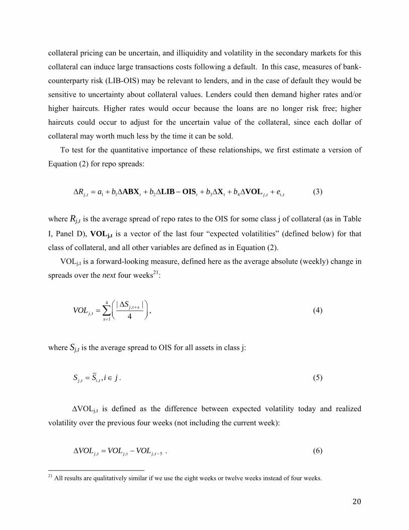
collateral pricing can be uncertain, and illiquidity and volatility in the secondary markets for this

collateral can induce large transactions costs following a default. In this case, measures of bank-

counterparty risk (LIB-OIS) may be relevant to lenders, and in the case of default they would be

sensitive to uncertainty about collateral values. Lenders could then demand higher rates and/or

higher haircuts. Higher rates would occur because the loans are no longer risk free; higher

haircuts could occur to adjust for the uncertain value of the collateral, since each dollar of

collateral may worth much less by the time it can be sold.

To test for the quantitative importance of these relationships, we first estimate a version of

Equation (2) for repo spreads:

ΔRj ,t = a1 + b1ΔABXt + b2ΔLIB − OISt + b3ΔXt + b4ΔVOL j ,t + ei,t (3)

where Rj,t is the average spread of repo rates to the OIS for some class j of collateral (as in Table

I, Panel D), VOLj,t is a vector of the last four “expected volatilities” (defined below) for that

class of collateral, and all other variables are defined as in Equation (2).

VOLj,t is a forward-looking measure, defined here as the average absolute (weekly) change in

spreads over the next four weeks21:

VOLj ,t =| ΔSj ,t+ s |

4⎛⎝⎜

⎞⎠⎟s=1

4

∑ , (4)

where Sj,t is the average spread to OIS for all assets in class j:

Sj ,t = Si,t , i ∈ j . (5)

ΔVOLj,t is defined as the difference between expected volatility today and realized

volatility over the previous four weeks (not including the current week):

ΔVOLj ,t = VOLj ,t −VOLj ,t−5 . (6)

                                                        21 All results are qualitatively similar if we use the eight weeks or twelve weeks instead of four weeks.

  21

Note that volatility uses absolute differences, and not percentage differences, because

percentage differences are harder to interpret across multiple weeks. Also, since we use future

information for our expected-volatility proxy, the resulting estimates could not be part of an

implementable investment strategy. This restriction does not matter for our analysis, since we are

not seeking to build investment portfolios from these results. In any case, we don’t really have a

choice here, since there is no way to extract volatility expectations from historical spread data

alone.

We estimate (3) for all five classes of collateral that have data available to construct the VOL

measure.22 The regression results for these five classes are shown in Table V. The final rows

show the results of the F-tests for the joint significance of LIB-OIS (Test 1), the ABX (Test 2)

and VOL changes (Test 3), respectively. These tests show that the changes in repo spreads are

significantly related to the change in LIB-OIS for all five categories, with almost all of the effect

coming in the contemporaneous period. Changes in repo spreads are not significantly related to

changes in the ABX or VOL or to any of the other control variables. Thus, just as we found for

credit spreads in our earlier analysis, the state variable for bank-counterparty risk is the only

significant correlate with repo spreads.

It seems natural that banks would have to raise repo spreads to attract funds. But, higher rates

do not by themselves cause a systemic event. For a “run on repo”, we need to see that even

higher rates are insufficient to keep repo lenders in the market. Our simple illustrations of repo

haircuts in Section III showed that this did occur. We next explore the factors related to these

increases using the same regression framework as we did for repo spreads:

ΔH j ,t = a1 + b1ΔABXt + b2ΔLIB − OISt + b3ΔXt + b4ΔVOL j ,t + ei,t , (7)

where Hj,t is the average haircut for all assets in class j, and all other variables are defined as in

(3). Since haircuts are already defined as a percentage of the total value of the underlying

collateral, the change in haircuts on the left-hand-side of equation (7) is already given in

percentages. Table VI summarizes the results. As we have found in earlier tests, the ABX and

the control variables are not significant. In contrast to previous regressions, the change in the

                                                        22 For the other four classes of collateral shown in Panel D of Table I, we do not have data for the spreads of the underlying assets.

  22

LIB-OIS is also not significant. The only variable with any explanatory power is the proxy for

expected volatility, which is significant for three of the five classes of collateral.

The key finding here is that both repo spreads and repo haircuts rose during the crisis,

with these increases correlated either to concerns about counterparty risk (for spreads), or to

uncertainty about collateral values (for haircuts). While these results are somewhat different for

spreads and haircuts, we suspect that this system is jointly determined, and that a disruption in

the interbank market and increases in uncertainty about collateral are both necessary conditions

for a run on repo. In an environment with no counterparty risk, there is no reason to expect

haircuts to be affected by uncertainty about collateral; similarly, high counterparty risk by itself

would be unlikely to affect repo spreads if all collateral had fixed values and liquid markets. It

seems unlikely that nature will give us an example with rising VOL but no change in LIB-OIS.

Instead, all of these things happened at the same time, and it is not possible to disentangle the

exact causes.

V. Conclusion

How did problems in the subprime mortgages cause a systemic event? Our answer is that

there was a run in the repo market. The location and size of subprime risks held by counterparties

in the repo market were not known and led to fear that liquidity would dry up for collateral, in

particular non-subprime related collateral. Uncertainty led to increases in the repo haircuts,

which is tantamount to massive withdrawals from the banking system.

The banking system has changed, with “securitized banking” playing an increasing role

alongside traditional banking. One large area of securitized banking – the securitization of

subprime home mortgages – began to weaken in early 2007, and continued to decline throughout

2007 and 2008. But, the weakening of subprime per se was not the shock that caused systemic

problems. The first systemic event occurs in August 2007, with a shock to the repo market that

we demonstrate using the “LIB-OIS,” the spread between the LIBOR and the OIS, as a proxy.

The reason that this shock occurred in August 2007 – as opposed to any other month of 2007 – is

perhaps unknowable. We hypothesize that the market slowly became aware of the risks

associated with the subprime market, which then led to doubts about repo collateral and bank

solvency. At some point – August 2007 in this telling – a critical mass of such fears led to the

  23

first run on repo, with lenders no longer willing to provide short-term finance at historical

spreads and haircuts.

After August 2007, the securitized-banking model was under pressure, with small equity

bases stretched by increasing haircuts on high-grade collateral. We see evidence of this pressure

in the co-movement of spreads on a wide variety of AAA and AA credits. This pressure

contributed to the forced rescue of Bear Stearns in March 2008 and the failure of Lehman

Brothers In September 2008. The second systemic event and run on repo occurred with the

failure of Lehman. In this second event, we see parallels to 19th century banking crises, with a

famine of liquidity leading to significant premia on even the safest of assets.

  24

References

Acharya, Viral, Douglas Gale, and Tanju Yorulmazer (2009), Rollover risk and market freezes, New York University, working paper.

Almeida, Heitor, Murillo Campello, and Bruno Laranjeira (2009), “Corporate Debt Maturity and

the Real Effects of the 2007 Credit Crisis,” University of Illinois, working paper. Arora, Navneet, Priyank Gandhi, and Francis Longstaff (2009), “Counterparty Credit Risk and

the Credit Default Swap Market,” UCLA, working paper. Baba, Naohiko and Frank Packer (2009), “From Turmoil to Crisis: Dislocations in the FX Swap

Market Before and After the Failure of Lehman Brothers,” BIS Working Paper, No. 285. Bank for International Settlements (1999), “Implications of Repo Markets for Central Banks,”

Report of a Working Group established by the Committee on the Global Financial System of the Central Banks of the Group of Ten Countries, March 9, 1999.

Brunnermeier, Markus and Lasse H. Pedersen (2009), “Market Liquidity and Funding

Liquidity,” Review of Financial Studies 22(6), 2201-2238. Campello, Murillo, Erasmo Giabona, John Graham, and Campell Harvey (2009), “Liquidity

Management and Corporate Investment during a Financial Crisis,” Duke University, working paper.

Carey, Mark, Ricardo Correa, and Jason Kotter (2009), "Revenge of the Steamroller: ABCP as a

Window on Risk Choices," Board of Governors of the Federal Reserve System, working paper.

Coffey, Niall, Warren Hrung, and Asani Sarkar (2009), “Capital Constraints, Counterparty Risk

and Deviations from Covered Interest Rate Parity,” New York Federal Reserve Bank, working paper.

Collin-Dufresne, Pierre, Robert Goldstein, and Spencer Martin (2001), “The Determinants of

Credit Spread Changes,” Journal of Finance Vol. 56, No. 6: 2177-2207. Corrigan, Danny and Natasha de Terán (2007), Collateral: Securities Lending, Repo, OTC

Derivatives and the Future of Finance (Global Custodian; London).

  25

Covitz, Daniel, Nellie Liang, and Gustavo Suarez (2009), “The Evolution of a Financial Crisis: Runs in the Asset-Backed Commercial Paper Market,” Board of Governors of the Federal Reserve System, Working Paper No. 2009-36.

Dang, Tri Vi, Gary Gorton, and Bengt Holmström (2009), “Opacity and the Optimality of Debt

for Liquidity Provision,” working paper. Eichengreen, Barry, Ashoka Mody, Milan Nedeljkovic, and Lucio Sarno (2009), “How the

Subprime Crisis Went Global: Evidence from Bank Credit Default Swap Spreads,” NBER Working Paper 14904.

Fabozzi, Frank and Steven Mann (2000), Floating-Rate Securities (Wiley). Fender, Ingo and Martin Scheicher (2009), “The Pricing of Subprime Mortgage Risk in Good

Times and Bad: Evidence from the ABX.HE Indices,” BIS Working Papers, No. 279. Fishback, Price, William Horrace, and Shawn Kantor (2001), “The Origins of Modern Housing

Finance: The Impact of Federal Housing Programs during the Great Depression,” University of Arizona, working paper.

Fontana, Allessandro (2009), “The Persistent Negative CDS-bond Basis during the 2007/2008

Financial Crisis,” University of Ca' Foscari Venice, working paper. Geanakoplos, John (2009), “The Leverage Cycle,” Yale, Cowles Foundation Discussion Paper

No. 1715. Gorton, Gary (2009), “Information, Liquidity, and the (Ongoing) Panic of 2007,” American

Economic Review, Papers and Proceedings, vol. 99, no. 2, 567-572. Gorton, Gary (2008), The Panic of 2007,” in Maintaining Stability in a Changing Financial

System, Proceedings of the 2008 Jackson Hole Conference, Federal Reserve Bank of Kansas City, 2008.

Gorton, Gary "Clearinghouses and the Origin of Central Banking in the U.S.," Journal of

Economic History 45:2 (June 1985): 277-83. Gorton, Gary and Lixin Huang (2006), “Banking Panics and Endogenous Coalition Formation,”

Journal of Monetary Economics, Vol. 53 (7): 1613-1629.

  26

Gorton, Gary and Don Mullineaux (1987), "The Joint Production of Confidence: Endogenous Regulation and Nineteenth Century Commercial Bank Clearinghouses," Journal of Money, Credit and Banking 19(4): 458-68.

Gorton, Gary and Nicholas Souleles (2006), “Special Purpose Vehicles and Securitization,”

chapter in The Risks of Financial Institutions, edited by Rene Stulz and Mark Carey (University of Chicago Press).

Gorton, Gary and George Pennacchi (1995), "Banks and Loan Sales: Marketing Non-Marketable

Assets," Journal of Monetary Economics 35(3): 389-411. Gorton, Gary and George Pennacchi (1990), "Financial Intermediaries and Liquidity Creation,"

Journal of Finance 45:1 (March): 49-72. Gyntelberg, Jacob and Philip Wooldridge (2008), “Interbank Rate Fixings During the Recent

Turmoil,” Bank for International Settlements Quarterly Review (March), 59-72. He, Zhiguo and Wei Xiong (2009), “Dynamic Debt Runs,” Princeton University, Princeton,

Working paper. Hördahl, Peter and Michael King (2008), “Developments in Repo Markets During the Financial

Turmoil,” Bank for International Settlements Quarterly Review (December), 37-53. Investment Company Institute (2009), “Report of the Money Market Working Group,” (March 17,

2009). Ivashina, Victoria and David Scharfstein (2008), “Bank Lending during the Financial Crisis of

2008,” Working Paper, Harvard Business School. Pagano, M. and Volpin, P. 2008. “Securitization, Transparency, and Liquidity,” Working Paper. Reinhart, Carmen and Kenneth Rogoff (2008), “Is the 2007 U.S. Subprime Financial Crisis So

Different? An International Historical Comparison,” American Economic Review 98, 339-344.

Schwarz, Krista (2009), “Mind the Gap: Disentangling Credit and Liquidity Risk Spreads,”

Wharton School, working paper. Schweitzer, Lisa, Seth Grosshandler, and William Gao (2008), “Bankruptcy Court Rules that

Repurchase Agreements Involving Mortgage Loans are Safe Harbored Under the

  27

Bankruptcy Code, But That Servicing Rights Are Not,” Journal of Bankruptcy Law (May/June), 357- 360.

Shleifer, Andrei and Robert Vishny, 2009, “Unstable Banking”, NBER working paper 14943. Singh, Manmohan and James Aitken (2009), “Counterparty Risk, Impact on Collateral Flows,

and Role for Central Counterparties,” IMF Working Paper WP/09/173. Stanton, Richard and Nancy Wallace (2009), “The Bear’s Lair: Indexed Credit Default Swaps

and the Subprime Mortgage Crisis,” Berkeley, working paper.

  

  28

Appendix A: Glossary of Key Terms and Asset Classes

This glossary provides definitions for all terms given in bold in the body of the paper and

all asset classes listed in Table 1. For the latter group, we include the panel location of that

variable in parenthesis following the definition (e.g: Table I – Panel A).

AA-AAA ABS RMBS/CMBS: Residential mortgage-backed security (RMBS) or

commercial mortgage-backed security (CMBS) with ratings between AA and AAA, inclusive.

(Table I - Panel D)

<AA ABS RMBS-CMBS: Residential mortgage-backed security (RMBS) or

commercial mortgage-backed security (CMBS) with ratings between AA and AAA, inclusive.

(Table I - Panel D)

AA-AAA CDO: Collateralized debt obligations (CDO) with ratings between AA and

AAA, inclusive. (Table I - Panel D)

AA-AAA CLO: Collateralized loan obligations (CDO) with ratings between AA and

AAA, inclusive. (Table I - Panel D)

A-AAA ABS Auto/CC/SL: Asset-backed securities (ABS) comprised of auto loans,

credit-card receivables, or student loans, with ratings between A and AAA, inclusive. (Table I -

Panel D)

ABX, ABX Index, ABX Index Spread: The ABX Index is a credit derivative that references

20 equally-weighted subprime RMBS tranches. There are also sub-indices linked to a basket of

subprime bonds with specific ratings: AAA, AA, A BBB and BBB-. Each sub-index references

the 20 subprime RMBS bonds with the rating level of the subindex. Every six months the indices

are reconstituted based on a pre-identified set of rules, and a new vintage of the index and sub-

indices are issued. In this paper, we focus on the BBB ABX tranche of the first vintage of the

ABX in 2006, which is representative of the riskier levels of subprime securitization. We refer to

this tranche of the 2006-1 issue simply as “ABX”.

Asset-Backed Securities (ABS): An asset-backed security is a bond which is backed by

the cash flows from a pool of specified assets in a special purpose vehicle rather than the

general credit of a corporation. The asset pools may be residential mortgages, in which case it is

a residential mortgage-backed security (RMBS), commercial mortgages – a commercial

  29

mortgage-backed security (CMBS), automobile loans, credit card receivables, student loans,

aircraft leases, royalty payments, and many other asset classes.

Australia RMBS AAA: AAA-rated RMBS backed by Australian mortgages. (Table I –

Panel C)

Auto AAA: AAA-rated ABS backed by auto loans. (Table 1 – Panel B)

BBB+/A Corporates: Corporate bonds rated between BBB+ and A, inclusive. (Table I -

Panel D)

Cards AAA: AAA-rated ABS backed by credit-card receivables. (Table I – Panel B)

CMBS AAA: AAA-rated Commercial-mortgage-backed securities. (Table I – Panel

B)

Credit Default Swaps (CDS): A credit default swap is derivative contract in which one

party agrees to pay the other a fixed periodic coupon for the specified life of the agreement. The

other party makes no payments unless a specified credit event occurs. Credit events are typically

defined to include a material default, bankruptcy or debt restructuring for a specified reference

asset. If such a credit event occurs, the party makes a payment to the first party, and the swap

then terminates. The size of the payment is usually linked to the decline in the reference asset's

market value following the credit event.

Collateralized Debt Obligations (CDOs): A CDO is a special purpose vehicle, which

buys a portfolio of fixed income assets, and finances the purchase of the portfolio via issuing

different tranches of risk in the capital markets. These tranches are senior tranches, rated

Aaa/AAA, mezzanine tranches, rated Aa/AA to Ba/BB, and equity tranches (unrated). Of

particular interest are ABS CDOs, which have underlying portfolios consisting of asset-backed

securities (ABS), including residential mortgage-backed securities (RMBS) and commercial

mortgage-backed securities (CMBS).

Collateralized Loan Obligations (CLOs): A CLO is a securitization of commercial bank

loans.

Commercial Mortgage-backed Securities (CMBS): See asset-backed securities,

above.

Dutch RMBS AAA: AAA-rated RMBS backed by Dutch mortgages. (Table I – Panel C)

European Auto AAA: AAA-rated ABS backed by European auto loans (Table I – Panel

C)

  30

European Consumer Receivables AAA: AAA-rated ABS backed by European

consumer receivables (Table I – Panel C)

Haircut: The collateral pledged by borrowers towards the repo has a haircut or “initial

margin” applied, which means the collateral is valued at less than market value. This haircut

reflects the perceived underlying risk of the collateral and protects the lender against a change in

its value. Haircuts are different for different asset classes and ratings.

HEL BBB: BBB-rated ABS backed by Home-equity loans with BBB ratings (Table 1-

Panel A)

HELOC AAA: AAA-rated ABS backed by Home-equity lines-of-credit (Table I- Panel

A)

HG SF CDO (High-grade structured-finance CDOs): High-grade structured-finance

CDOs buy collateral consisting of the AAA and AA-rated tranches of securitized bonds. (Table 1

– Panel B)

Home-equity loans (HEL): A home equity loan is a line of credit under which a home

owner can borrower using the home equity as collateral.

Home-equity lines-of-credit (HELOC): A HELOC differs from a home equity loan in

that the borrower does not borrower the full amount of the loan at the outset, but can draw down

the line of credit over a specified period of time with a maximum amount.

LIB-OIS: The spread between the LIBOR and the OIS.

LIBOR: The London Interbank Offered Rate (LIBOR) is a series of interest rates, of

different maturities and currencies, at which banks offer to lend fund to each other. These rates

are calculated by the British Bankers’ Association as the averages of quotes contributed by a

panel of banks and announced at 11:00 Am local time in England. This is called the rate

“fixing.” Quotes are ranked and the top and bottom quartiles are discarded. LIBOR is fixed for

15 different maturities, from overnight to one year, and in ten international currencies. Similar

fixing arrangements exist in many markets around the world. See Gyntelberg and Wooldridge

(2008).

Mezzanine CDO: A Mezzanine CDO refers to a collateralized debt obligation where

the underlying portfolio consists of tranches of different asset-backed securities that are rated

between BBB and A, inclusive.

  31

Mezzanine SF CDO: Mezzanine structured-finance CDOs buy collateral consisting of

the A through BBB-rated tranches of securitized bonds. (Table I – Panel B)

Monoline Insurers, Monoline Insurance Companies (“monolines”): Insurance

companies that are restricted by regulation to one line of the business, the business of issuing

financial guarantees on bonds, that is insurance against the loss due to default of specified bonds.

The first such company was AMBAC Financial Group Inc., formed in 1971, followed by MBIA

formed in 1983. In 1989 a law in New York limited the sale of financial insurance products by

those companies solely to bond insurance, making them “monolines.”

Mortgage Originators: Financial firms that underwrite and fund residential and possibly

commercial, mortgages.

OIS: See Overnight Index Swap (Table I – Panel E).

Overnight Index Swap (OIS): An Overnight Indexed Swap (OIS) is a fixed/floating

interest rate swap where the floating leg of the swap is tied to a published index of a daily

overnight rate reference. The term ranges from one week to two years (sometimes more). At

maturity, the two parties agree to exchange the difference between the interest accrued at the

agreed fixed rate and interest accrued through geometric averaging of the floating index rate on

the agreed notional amount. This means that the floating rate calculation replicates the accrual on

an amount (principal plus interest) rolled at the index rate every business day over the term of the

swap. If cash can be borrowed by the swap receiver on the same maturity as the swap and at the

same rate and lent back every day in the market at the index rate, the cash payoff at maturity will

exactly match the swap payout: the OIS acts as a perfect hedge for a cash instrument. Since

indices are generally constructed on the basis of the average of actual transactions, the index is

generally achievable by borrowers and lenders. Economically, receiving the fixed rate in an OIS

is like lending cash. Paying the fixed rate in an OIS is like borrowing cash. Settlement occurs net

on the earliest practical date. There is no exchange of principal. The index rate used is typically

the weighted average rate for overnight transactions as published by the central bank (e.g., the

effective fed funds rate).

Repo-Haircut Index: The equal-weighted average haircut for all nine of the asset classes

in Panel D of Table I. Haircuts of 100% (= no trade) are included in this average. (Table I, Panel

D)

  32

Repo-Rate Index: During the time that all asset classes have active repo markets in 2007

and early 2008, this index is identical to the equal-weighted average repo rate for all nine the

asset classes in Panel D of Table I. As haircuts rise to 100% for any given asset class (= no

trade) on date t, we drop that class from the index and compute the index change for period t

using only the classes that traded in both period t-1 and period t. (Table I, Panel D)

Repurchase Agreements (repo), Reverse Repurchase Agreements (reverse repo): A

sale and repurchase agreement, known as a “repo” for short, is a sale of a security combined with

an agreement to repurchase the same security at a specified price at the end of the contract.

Economically, a repo is a secured or collateralized loan, that is, a loan of cash against a security

as collateral. From the point of view of the borrower of the cash (who is putting up the security

as collateral), it is a reverse repurchase agreement, or “reverse repo.”

Residential Mortgage-backed Security (RMBS): See asset-backed securities, above.

Securitization: The process of financing by segregating specified cash flows, from loans

originated by a firm (the “sponsor”) and selling claims specifically linked to these specified cash

flows. This is accomplished by setting up another company, called a special purpose vehicle

(SPV) or special purpose entity, and then selling the specified cash flows to this company, which

purchases the rights to the cash flows by issuing (rated) securities into the capital market. The

sponsor services the cash flows, that is, makes sure that the cash flows are arriving, etc. The SPV

is not an operating company in the usual sense. It is more of a robot company in that it is a set of

rules. It has no employees or physical location.

Securitized Banking: Refers in this paper to the nexus of securitization and repurchase

markets where “depositors” are able to engage in (reverse) repo by depositing money in

exchange for securitized bonds as collateral.

Securitized Bonds: A general term referring to any traded and rated tranche of an ABS,

RMBS, CMBS, CDO, or CLO.

Special Purpose Vehicle (SPV): An SPV or special purpose entity (SPE) is a legal entity

which has been set up for a specific, limited, purpose by another entity, the sponsoring firm. An

SPV can take the form of a corporation, trust, partnership, or a limited liability company. The

SPV may be a subsidiary of the sponsoring firm, or it may be an “orphan” SPV, one that is not

consolidated with the sponsoring firm for tax, accounting, or legal purposes (or may be

consolidated for some purposes but not others). An SPV can only carry out some specific

  33

purpose, or circumscribed activity, or a series of such transactions. An essential feature of an

SPV is that it be “bankruptcy remote,” that is, that the SPV never be able to become legally

bankrupt. The most straightforward way to achieve this would be for the SPV to waive its right

to file a voluntary bankruptcy petition, but this is legally unenforceable. The only way to

completely eliminate the risk of either voluntary or involuntary bankruptcy is to create the SPV

in a legal form that is ineligible to be a debtor under the U.S. Bankruptcy Code.

Structured Finance: A broad term used to describe securitized bonds, but also more

generally any bond with an embedded derivative.

Student AAA: AAA-rated ABS backed by student loans. (Table I – Panel B)

Tranche: A tranche (French for “cut”) refers to a slice of an portfolio ordered by

seniority, e.g., a senior tranche or AAA tranche is more senior than a junior tranche or BBB-

rated tranche.

UK Cards AAA: AAA-rated ABS backed by UK credit-card receivables (Table I –

Panel C)

UK RMBS AAA: AAA-rated RMBS backed by UK mortgages. (Table I – Panel C)

Unpriced ABS/MBS, All Subprime: All tranches of ABS, MBS and all subprime

securitized bonds which do not have public pricing posted on Bloomberg or Reuters (two news

services used by traders) (Table I ‐ Panel D)

Unpriced CDO/CLO: All tranches of CDO and CLO securitized bonds which do not

have public pricing posted on Bloomberg or Reuters (two news services used by traders) (Table 

I ‐ Panel D) 

VIX:  VIX is the ticker symbol for a measure of implied volatility from S&P 500 index 

options. A high value of the VIX is associated with a more violatile market and more costly 

options.  The VIX is calculated and traded on the Chicago Board Options Exchange.  (Table I 

– Panel E) 

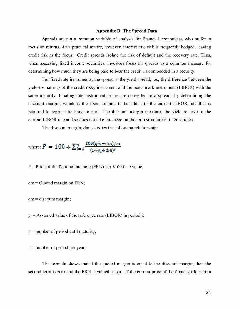
  34

Appendix B: The Spread Data

Spreads are not a common variable of analysis for financial economists, who prefer to

focus on returns. As a practical matter, however, interest rate risk is frequently hedged, leaving

credit risk as the focus. Credit spreads isolate the risk of default and the recovery rate. Thus,

when assessing fixed income securities, investors focus on spreads as a common measure for

determining how much they are being paid to bear the credit risk embedded in a security.

For fixed rate instruments, the spread is the yield spread, i.e., the difference between the

yield-to-maturity of the credit risky instrument and the benchmark instrument (LIBOR) with the

same maturity. Floating rate instrument prices are converted to a spreads by determining the

discount margin, which is the fixed amount to be added to the current LIBOR rate that is

required to reprice the bond to par. The discount margin measures the yield relative to the

current LIBOR rate and so does not take into account the term structure of interest rates.

The discount margin, dm, satisfies the following relationship:

where:

P = Price of the floating rate note (FRN) per $100 face value;

qm = Quoted margin on FRN;

dm = discount margin;

yi = Assumed value of the reference rate (LIBOR) in period i;

n = number of period until maturity;

m= number of period per year.

The formula shows that if the quoted margin is equal to the discount margin, then the

second term is zero and the FRN is valued at par. If the current price of the floater differs from

  35

par, then the discount margin is nonzero. The discount margin assumes that the cash flows over

the remaining life of the bond are determined by the current reference rate value. The margin is

selected so that the present value of the cash flows is equal to the security’s price. The discount

margin is a measure which is similar to yield-to-maturity for fixed rate instruments. It expresses

the price of an FRN relative to the current LIBOR level. See Fabozzi and Mann (2000).

  36

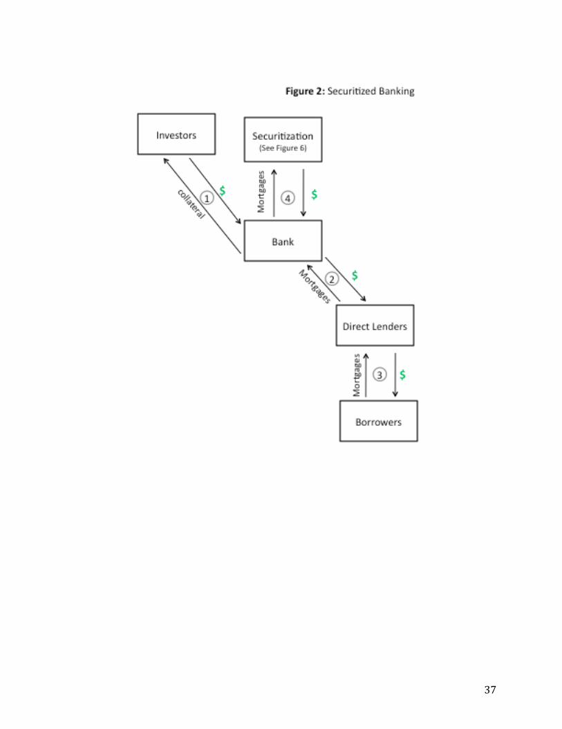
  37

  38

  39

Figure 4: The Repo-Haircut Index

Notes: The repo-haircut index is the equally-weighted average haircut for all nine asset classes

included in Table I, Panel D.

  40

Figure 5: Issuance in U.S. Capital Markets ($ billions)

Sources: U.S. Department of Treasury, Federal Agencies, Thomson Financial, Inside MBS & ABS, Bloomberg.

 

  41

 

  42

FIGURE 7

Source: Federal Flow of Funds.

  43

FIGURE 8: ABX vs. LIB-OIS

Notes: ABX is the 2006-1 BBB tranche. LIB-OIS spreads on left-hand Y-axis, ABX spreads on right-hand y-axis. Both scales are in basis points.

  44

Figure 9: LIB-OIS and Non-Subprime-Related Asset Classes

Notes: LIB-OIS is shown with the spreads on AAA-rated asset-backed securities: student loans, credit cards, and auto loans. The scale is in basis points.

  45

Table I Summary Statistics

This table reports the summary statistics for the state variable, credit spreads, repo spreads and control variables used in this paper. For each series we show summary statistics for the whole period and four subperiods. Panel A shows statistics for the state variable LIB-OIS and the credit spreads of three categories of subprime related assets. Panel B and Panel C shows statistics for the credit spreads of U.S. and non-U.S. non-subprime asset classes. Panel D reports the statistics for the spreads between three-month repo rates and OIS. Panel E shows statistics for the five control variables used in the regression analysis. All variables given in this Table are defined in Appendix A. All spreads are measured in basis points, with spread computations explained in Appendix B.

Panel A: State Variable and Subprime Related Assets Class Series Periods Mean Median Std. Err. Max Min

State Variable

LIB-OIS Spread

Whole period 72.43 66.44 67.57 354.20 7.45 First half of 2007 7.97 7.88 0.42 9.15 7.45

Second half of 2007 58.71 60.78 28.64 104.73 7.70 All of 2007 33.34 8.50 32.53 104.73 7.45 All of 2008 108.10 77.20 71.61 354.20 24.33 Credit Spreads of Sub-prime Related Assets

HEL BBB

Whole period 714.25 425.00 545.26 1800.00 170.00 First half of 2007 273.27 250.00 93.54 425.00 170.00

Second half of 2007 1113.46 1000.00 441.03 1800.00 350.00 All of 2007 693.37 425.00 528.75 1800.00 170.00

Mezzanine CDO BBB

Whole period 2861.93 2969.42 2023.57 8421.76 365.00 First half of 2007 627.50 650.00 152.50 950.00 365.00

Second half of 2007 2178.47 1940.75 659.41 3063.16 1100.00 All of 2007 1402.99 1025.00 915.27 3063.16 365.00 All of 2008 4858.38 4687.97 1268.88 8421.76 3016.83

HELOC AAA

Whole Period 121.60 18.00 157.64 500.00 14.00 First half of 2007 15.35 15.00 1.23 18.00 14.00

Second half of 2007 213.31 195.00 159.59 500.00 15.00 All of 2007 114.33 18.00 149.92 500.00 14.00 CDS Spreads of Subprime Mortgage Lenders

Countrywide

Whole period 275.86 220.02 253.96 1185.84 22.52 First half of 2007 51.10 50.79 17.64 77.57 22.52

Second half of 2007 445.43 282.34 338.99 1088.00 62.53 All of 2007 248.26 71.09 310.03 1088.00 22.52 All of 2008 301.04 260.00 188.39 1185.84 95.67

WAMU

Whole period 413.57 318.33 643.09 4352.43 19.61 First half of 2007 35.39 33.68 11.11 57.38 19.61

Second half of 2007 189.27 122.03 133.36 438.47 42.55 All of 2007 112.33 50.32 121.71 438.47 19.61 All of 2008 815.23 438.90 818.44 4352.43 255.00

CDS Spreads of Monoline Insurers

MBIA

Whole period 911.33 391.88 1116.88 4153.55 13.46 First half of 2007 24.20 22.66 9.34 42.20 13.46

Second half of 2007 164.92 121.69 89.44 322.96 45.18 All of 2007 94.56 43.69 94.93 322.96 13.46 All of 2008 1656.46 1391.26 1101.33 4153.55 372.55

MGIC

Whole period 520.96 453.46 406.35 1411.73 27.48 First half of 2007 51.42 52.40 17.82 81.32 27.48

Second half of 2007 270.97 245.95 138.90 528.53 71.21 All of 2007 161.20 79.09 147.99 528.53 27.48 All of 2008 849.17 885.61 262.06 1411.73 320.00

Radian

Whole period 1072.85 809.83 956.80 3164.27 28.53 First half of 2007 56.54 55.49 18.12 93.39 28.53

Second half of 2007 536.20 559.22 261.37 1000.32 73.26 All of 2007 296.37 86.62 303.80 1000.32 28.53 All of 2008 1781.22 1938.22 781.58 3164.27 704.70

  46

Panel B:U.S. Non-Subprime Asset Classes Series Periods Mean Median Std. Err. Max Min

Auto AAA

Whole period 109.42 55.00 153.65 500.00 -1.00 First half of 2007 -1.00 -1.00 0.00 -1.00 -1.00

Second half of 2007 23.38 20.00 16.11 50.00 -1.00 All of 2007 11.19 -1.00 16.70 50.00 -1.00 All of 2008 199.04 110.00 167.75 500.00 50.00

Cards AAA

Whole period 101.92 55.00 148.93 550.00 -4.00 First half of 2007 -3.31 -3.00 0.47 -3.00 -4.00

Second half of 2007 24.88 23.00 17.73 55.00 -3.00 All of 2007 10.79 -3.00 18.89 55.00 -4.00 All of 2008 185.05 100.00 166.45 550.00 50.00

Student AAA

Whole period 65.11 30.00 90.47 325.00 -3.00 First half of 2007 -1.12 -1.00 1.18 0.00 -3.00

Second half of 2007 17.92 18.00 10.28 35.00 0.00 All of 2007 8.40 0.00 12.03 35.00 -3.00 All of 2008 116.84 65.00 99.71 325.00 25.00

CMBS AAA

Whole period 241.16 123.00 313.92 1350.00 22.00 First half of 2007 26.27 26.50 2.79 31.00 22.00

Second half of 2007 65.88 62.00 21.83 105.00 31.50 All of 2007 46.08 31.25 25.25 105.00 22.00 All of 2008 419.12 250.00 349.14 1350.00 83.00

HG SF CDO AAA

Whole period 482.24 428.32 424.87 1463.10 23.00 First half of 2007 23.73 23.00 2.68 35.00 23.00

Second half of 2007 177.88 108.09 135.50 450.90 42.00 All of 2007 100.81 38.50 122.72 450.90 23.00 All of 2008 830.22 849.77 275.79 1463.10 391.43

Mezzanine SF CDO AAA

Whole period 1094.17 1084.79 873.46 2712.79 32.00 First half of 2007 54.38 55.00 20.99 105.00 32.00

Second half of 2007 567.96 444.69 380.54 1084.79 115.00 All of 2007 311.17 110.00 372.07 1084.79 32.00 All of 2008 1808.49 1742.65 506.59 2712.79 1006.25

Panel C: Non-US Non-Subprime Asset Classes

Australia RMBS AAA

Whole period 145.60 90.00 151.22 650.00 5.00 First half of 2007 6.23 7.00 0.91 7.00 5.00

Second half of 2007 48.15 50.00 24.66 90.00 5.00 All of 2007 27.19 7.00 27.32 90.00 5.00 All of 2008 257.55 200.00 133.86 650.00 90.00

UK RMBS AAA

Whole period 124.53 80.00 131.25 440.00 4.00 First half of 2007 4.96 5.00 0.72 6.00 4.00

Second half of 2007 45.15 50.00 22.23 80.00 5.00 All of 2007 25.06 6.00 25.58 80.00 4.00 All of 2008 218.58 180.00 121.08 440.00 80.00

Dutch RMBS AAA

Whole Period 56.56 50.00 42.40 170.00 10.00 First half of 2007 10.69 11.00 0.74 12.00 10.00

Second half of 2007 40.35 39.00 18.96 70.00 11.00 All of 2007 25.52 12.00 20.02 70.00 10.00 All of 2008 97.95 90.00 25.38 170.00 60.00

UK Cards AAA

Whole period 178.62 150.00 176.97 625.00 10.00 First half of 2007 10.08 10.00 0.28 11.00 10.00

Second half of 2007 44.38 40.00 25.94 90.00 11.00 All of 2007 32.95 27.00 26.67 90.00 10.00 All of 2008 281.91 215.00 165.05 625.00 90.00

European Consumer Receivable AAA

Whole period 206.25 200.00 176.36 600.00 15.00 First half of 2007 15.29 15.00 0.76 17.00 15.00

Second half of 2007 54.92 55.00 25.05 95.00 18.00 All of 2007 46.52 50.00 27.59 95.00 15.00 All of 2008 302.09 235.00 157.19 600.00 95.00

European Auto AAA

Whole period 120.57 85.00 119.56 450.00 7.00 First half of 2007 7.14 7.00 0.38 8.00 7.00

Second half of 2007 37.31 35.00 18.62 65.00 8.00 All of 2007 30.91 30.00 20.68 65.00 7.00 All of 2008 174.36 115.00 122.14 450.00 60.00

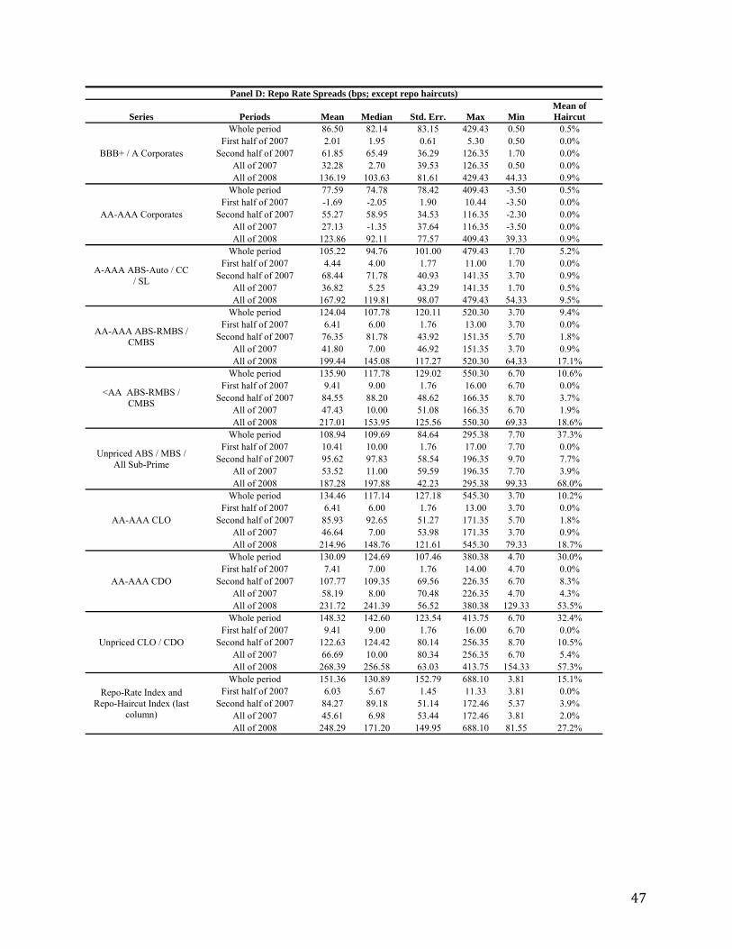
  47

Panel D: Repo Rate Spreads (bps; except repo haircuts)

Series Periods Mean Median Std. Err. Max Min Mean of Haircut

BBB+ / A Corporates

Whole period 86.50 82.14 83.15 429.43 0.50 0.5% First half of 2007 2.01 1.95 0.61 5.30 0.50 0.0%

Second half of 2007 61.85 65.49 36.29 126.35 1.70 0.0% All of 2007 32.28 2.70 39.53 126.35 0.50 0.0% All of 2008 136.19 103.63 81.61 429.43 44.33 0.9%

AA-AAA Corporates

Whole period 77.59 74.78 78.42 409.43 -3.50 0.5% First half of 2007 -1.69 -2.05 1.90 10.44 -3.50 0.0%

Second half of 2007 55.27 58.95 34.53 116.35 -2.30 0.0% All of 2007 27.13 -1.35 37.64 116.35 -3.50 0.0% All of 2008 123.86 92.11 77.57 409.43 39.33 0.9%

A-AAA ABS-Auto / CC / SL

Whole period 105.22 94.76 101.00 479.43 1.70 5.2% First half of 2007 4.44 4.00 1.77 11.00 1.70 0.0%

Second half of 2007 68.44 71.78 40.93 141.35 3.70 0.9% All of 2007 36.82 5.25 43.29 141.35 1.70 0.5% All of 2008 167.92 119.81 98.07 479.43 54.33 9.5%

AA-AAA ABS-RMBS / CMBS

Whole period 124.04 107.78 120.11 520.30 3.70 9.4% First half of 2007 6.41 6.00 1.76 13.00 3.70 0.0%

Second half of 2007 76.35 81.78 43.92 151.35 5.70 1.8% All of 2007 41.80 7.00 46.92 151.35 3.70 0.9% All of 2008 199.44 145.08 117.27 520.30 64.33 17.1%

<AA ABS-RMBS / CMBS

Whole period 135.90 117.78 129.02 550.30 6.70 10.6% First half of 2007 9.41 9.00 1.76 16.00 6.70 0.0%

Second half of 2007 84.55 88.20 48.62 166.35 8.70 3.7% All of 2007 47.43 10.00 51.08 166.35 6.70 1.9% All of 2008 217.01 153.95 125.56 550.30 69.33 18.6%

Unpriced ABS / MBS / All Sub-Prime

Whole period 108.94 109.69 84.64 295.38 7.70 37.3% First half of 2007 10.41 10.00 1.76 17.00 7.70 0.0%

Second half of 2007 95.62 97.83 58.54 196.35 9.70 7.7% All of 2007 53.52 11.00 59.59 196.35 7.70 3.9% All of 2008 187.28 197.88 42.23 295.38 99.33 68.0%

AA-AAA CLO

Whole period 134.46 117.14 127.18 545.30 3.70 10.2% First half of 2007 6.41 6.00 1.76 13.00 3.70 0.0%

Second half of 2007 85.93 92.65 51.27 171.35 5.70 1.8% All of 2007 46.64 7.00 53.98 171.35 3.70 0.9% All of 2008 214.96 148.76 121.61 545.30 79.33 18.7%

AA-AAA CDO

Whole period 130.09 124.69 107.46 380.38 4.70 30.0% First half of 2007 7.41 7.00 1.76 14.00 4.70 0.0%

Second half of 2007 107.77 109.35 69.56 226.35 6.70 8.3% All of 2007 58.19 8.00 70.48 226.35 4.70 4.3% All of 2008 231.72 241.39 56.52 380.38 129.33 53.5%

Unpriced CLO / CDO

Whole period 148.32 142.60 123.54 413.75 6.70 32.4% First half of 2007 9.41 9.00 1.76 16.00 6.70 0.0%

Second half of 2007 122.63 124.42 80.14 256.35 8.70 10.5% All of 2007 66.69 10.00 80.34 256.35 6.70 5.4% All of 2008 268.39 256.58 63.03 413.75 154.33 57.3%

Repo-Rate Index and Repo-Haircut Index (last

column)

Whole period 151.36 130.89 152.79 688.10 3.81 15.1% First half of 2007 6.03 5.67 1.45 11.33 3.81 0.0%

Second half of 2007 84.27 89.18 51.14 172.46 5.37 3.9% All of 2007 45.61 6.98 53.44 172.46 3.81 2.0% All of 2008 248.29 171.20 149.95 688.10 81.55 27.2%

  48

Panel E: Control variables Series Periods Mean Median Std. Err. Max Min

ABX Index (bps)

Whole period 4090.11 3604.00 3524.76 10940.98 121.00 First half of 2007 302.15 329.50 139.54 552.00 121.00

Second half of 2007 1657.69 1752.00 894.91 3286.00 368.00 All of 2007 979.92 481.50 933.01 3286.00 121.00 All of 2008 6927.48 6938.67 2447.64 10940.98 3373.00

10Year Treasury Rate

Whole period 4.07% 4.04% 0.71% 5.19% 2.08% First half of 2007 4.77% 4.73% 0.20% 5.19% 4.51%

Second half of 2007 4.52% 4.51% 0.32% 5.14% 3.96% All of 2007 4.64% 4.66% 0.29% 5.19% 3.96% All of 2008 3.56% 3.72% 0.56% 4.50% 2.08%

OIS

Whole period 3.26% 3.53% 1.79% 5.29% 0.18% First half of 2007 5.28% 5.28% 0.01% 5.29% 5.26%

Second half of 2007 4.65% 4.60% 0.42% 5.28% 4.07% All of 2007 4.96% 5.27% 0.43% 5.29% 4.07% All of 2008 1.70% 2.00% 0.94% 3.96% 0.18%

Return of S&P 500

Whole period -0.40% 0.20% 3.83% 17.97% -18.34% First half of 2007 0.25% 0.18% 1.45% 3.04% -3.65%

Second half of 2007 -0.06% 0.01% 2.02% 3.74% -4.53% All of 2007 0.09% 0.18% 1.75% 3.74% -4.53% All of 2008 -0.85% 0.22% 4.98% 17.97% -18.34%

VIX

Whole period 25.94 22.49 14.93 80.86 10.18 First half of 2007 13.05 13.07 1.97 17.06 10.18

Second half of 2007 21.88 21.2 4.02 30.83 15.23 All of 2007 17.47 15.68 5.45 30.83 10.18 All of 2008 33.68 25.59 16.59 80.86 16.3

Slope of Yield Curve

Whole period 1.01% 1.22% 0.78% 2.62% -0.13% First half of 2007 -0.02% -0.04% 0.09% 0.22% -0.13%

Second half of 2007 0.59% 0.55% 0.31% 1.39% 0.17% All of 2007 0.29% 0.18% 0.38% 1.39% -0.13% All of 2008 1.66% 1.57% 0.34% 2.62% 1.08%

  49

Table II Credit Spreads Regression Results

For each bond i, we estimate equation (2) using weekly data from January 4, 2007 to January 29, 2009, ∆LIB-OIS is the percentage change of the spread between the 3-month LIBOR and the Overnight Index Swap (OIS). ∆ABX is the parentage change of the ABX index at period t. ∆OIS is the Overnight Index Swap. ∆r-10 is the change in yield on the 10-year Treasury, with its square given by (∆r-10)^2. ∆Slope is the change in 10-year minus 2-year Treasury yields. ∆VIX is the change in implied volatility of S&P 500, and ∆S&P is the return on S&P 500. t-statistics are given in parentheses below the coefficient estimates. The last two rows report F-statistics and p-values for the key state variables. The null hypothesis of the LIB-OIS F-Test is that the sum of all coefficients of ∆LIB-OIS and its lags is zero. The null hypothesis of the ABX F-Test is the sum of all coefficients of ∆ABX and its lags is zero. Panel A shows the results of six U.S. non-subprime assets and Panel B shows the results of six non-US non-subprime assets.

Panel A: U.S. Non-Subprime Asset Classes Credit Spreads

Cards Auto Student CMBS HG SF CDO

Mezz SF CDO

Intercept 0.003 0.016 -0.010 0.036 0.042 0.052 (0.1) (0.33) (-0.33) (2.41) (2.86) (3.96)

∆LIB-OIS 0.341 0.079 0.461 0.025 -0.051 -0.037 (3.24) (0.54) (5.23) (0.26) (-1.16) (-0.94)

∆LIB-OIS, t-1 0.264 0.486 0.131 0.078 -0.042 0.055 (2.64) (3.55) (1.59) (0.84) (-1.00) (1.45)

∆LIB-OIS, t-2 0.132 0.012 0.138 -0.082 0.038 -0.081 (1.32) (0.08) (1.67) (-0.92) (0.91) (-2.15)

∆LIB-OIS, t-3 0.027 0.170 -0.013 -0.030 -0.030 -0.004 (0.27) (1.25) (-0.16) (-0.33) (-0.72) (-0.1)

∆ABX -0.141 -0.331 0.455 0.012 0.001 0.070 (-0.66) (-1.13) (2.32) (0.27) (0.00) (0.86)

∆ABX, t-1 0.079 -0.025 0.119 -0.013 0.016 0.061 (0.36) (-0.09) (0.6) (-0.32) (0.18) (0.74)

∆ABX, t-2 0.315 0.250 -0.202 -0.072 -0.020 -0.040 (1.48) (0.86) (-1.06) (-1.71) (-0.23) (-0.5)

∆ABX, t-3 -0.277 -0.351 -0.150 -0.052 0.049 -0.011 (-1.3) (-1.2) (-0.69) (-1.24) (0.54) (-0.14)

∆OIS -0.253 -0.147 -0.358 -0.096 0.156 0.106 (-0.78) (-0.33) (-1.34) (-0.69) (1.14) (0.85)

∆r-10 0.111 -0.092 0.059 -0.214 -0.227 -0.132 (0.58) (-0.36) (0.36) (-2.65) (-2.87) (-1.85)

(∆r-10)^2 0.174 0.076 0.037 -0.042 -0.094 -0.144 (0.57) (0.18) (0.14) (-0.33) (-0.75) (-1.26)

∆S&P -0.443 1.518 -0.757 -1.622 -0.580 0.592 (-0.29) (0.7) (-0.57) (-2.42) (-0.89) (0.99)

∆VIX -0.006 0.004 -0.003 0.003 0.002 0.006 (-0.5) (0.23) (-0.29) (0.56) (0.41) (1.26)

∆Slope -0.155 0.189 -0.039 0.298 0.269 0.075 (-0.74) (0.64) (-0.23) (3.29) (3.02) (0.92)

LIB-OIS F-test 20.16 10.26 26.13 2.99 1.38 1.08 (<0.01) (<0.01) (<0.01) (0.08) (0.24) (0.30)

ABX F-test 0.00 0.73 0.42 0.00 0.08 0.39 (0.95) (0.40) (0.52) (0.95) (0.78) (0.59)

 

  50

Panel B: Non-US Non-Subprime Asset Classes Credit Spreads

Australia RMBS UK RMBS

Dutch RMBS UK Cards

European Consumer Receivable

European Auto

Intercept 0.014 0.017 0.014 0.031 0.032 0.037 (0.52) (0.93) (1.14) (2.4) (3.21) (2.35) ∆LIB-OIS 0.126 0.240 0.100 0.109 0.049 0.081

(1.57) (4.38) (2.71) (2.86) (1.76) (1.8) ∆LIB-OIS, t-1 0.575 0.237 0.071 0.136 0.021 0.019

(7.56) (4.57) (2.11) (3.72) (0.8) (0.45) ∆LIB-OIS, t-2 -0.181 -0.051 0.115 0.019 0.033 0.104

(-2.44) (-1.01) (3.42) (0.52) (1.26) (2.51) ∆LIB-OIS, t-3 0.138 0.067 -0.015 -0.019 0.020 0.022

(1.86) (1.32) (-0.47) (-0.55) (0.77) (0.53) ∆ABX 0.025 0.029 0.095 0.094 0.116 0.095

(0.15) (0.26) (1.37) (1.03) (1.65) (0.84) ∆ABX, t-1 -0.002 0.022 0.002 0.028 0.001 -0.010

(-0.02) (0.19) (0.03) (0.34) (0.01) (-0.09) ∆ABX, t-2 -0.171 -0.018 -0.037 0.011 0.037 0.044

(-1.09) (-0.17) (-0.54) (0.13) (0.54) (0.4) ∆ABX, t-3 0.173 0.072 -0.109 -0.084 -0.060 -0.265

(1.09) (0.66) (-1.6) (-1.05) (-0.9) (-2.47) ∆OIS 0.034 -0.031 -0.237 -0.051 -0.054 -0.164

(0.1) (-0.15) (-0.63) (-0.33) (-0.48) (-0.91) ∆r-10 -0.207 -0.140 -0.067 -0.134 -0.106 -0.146

(-1.36) (-1.34) (-0.81) (-1.84) (-1.97) (-1.71) (∆r-10)^2 0.194 -0.022 -0.058 -0.036 -0.096 -0.018

(0.85) (-0.15) (-0.5) (-0.34) (-1.23) (-0.15) ∆S&P -0.915 -0.272 -0.709 0.164 0.194 0.695

(-0.76) (-0.33) (-0.86) (0.28) (0.45) (1.01) ∆VIX -0.006 -0.001 -0.002 0.000 0.001 0.003

(-0.64) (-0.11) (-0.31) (0.07) (0.39) (0.6) ∆Slope 0.179 0.077 0.051 0.133 0.091 0.190

(1.05) (0.66) (0.51) (1.64) (1.53) (2) LIB-OIS 25.57 30.71 20.89 14.40 6.56 8.62

F-test (<0.01) (<0.01) (<0.01) (<0.01) (0.01) (<0.01) ABX 0.01 0.28 0.14 0.09 0.51 0.41 F-test (0.93) (0.60) (0.71) (0.77) (0.48) (0.52)

  51

Table III Summary of F-Test Results for Different Asset Categories 

For each bond i, we estimate equation (2) using weekly data from January 4, 2007 to January 29, 2009, ∆LIB-OIS is the percentage change of the spread between the 3-month LIBOR and the Overnight Index Swap (OIS). This table summarizes the F-test results for the LIB-OIS state variable and its lags. The null hypothesis of F-test is the sum of all coefficients of ∆LIB-OIS and its lags is zero. The numbers in the table indicate how many F-tests of bonds in each category are significant at various confidence levels. Asset categories are listed in Panel A of Table I. “Negative” and “Positive” indicate the sign of the sum of coefficients for ∆LIB-OIS and its lags.

Panel A: Whole Period: January 4, 2007 to January 29, 2009

Negative Positive Categories Total Number 10% 5% 1% 10% 5% 1% Subprime 63 1 1 0 2 1 2

Nonsubprime_US 176 3 0 0 4 7 106 Nonsubprime_Europe 59 0 0 0 0 6 39

Financial 46 0 0 0 3 2 6 Industrial 48 0 0 0 5 14 9

Total 392 4 1 0 14 30 162

Panel B: Subperiod I: January 4, 2007 to December 27, 2007

Negative Positive Categories Total Number 10% 5% 1% 10% 5% 1% Subprime 63 2 4 2 0 2 1

Nonsubprime_US 176 4 0 1 8 21 75 Nonsubprime_Europe 59 0 0 0 5 10 24

Financial 46 3 1 0 1 2 1 Industrial 48 0 0 0 0 1 4

Total 392 9 5 3 14 36 105

Panel C: Subperiod II: January 3, 2008 to January 29,2009

Negative Positive Categories Total Number 10% 5% 1% 10% 5% 1% Subprime 63 1 0 0 0 0 0

Nonsubprime_US 176 8 0 0 23 26 41 Nonsubprime_Europe 59 0 0 0 0 1 0

Financial 46 0 0 0 6 10 6 Industrial 48 0 0 0 6 9 21

Total 392 9 0 0 35 46 68

  52

 Table IV Summary of F-Test Results for Different Rating Classes

For each bond i, we estimate equation (2) using weekly data from January 4, 2007 to January 29, 2009, ∆LIB-OIS is the percentage change of the spread between the 3-month LIBOR and the Overnight Index Swap (OIS).This table summarizes the F-test results for the LIB-OIS state variable and its lags. The null hypothesis of F-test is the sum of all coefficients of ∆LIB-OIS and its lags is zero. The numbers in the table indicate how many F-tests of bonds in each rating class are significant at various confidence levels. “Negative” and “Positive” indicate the sign of the sum of the coefficients for ∆LIB-OIS and its lags.

Panel A: Whole Period: January 4, 2007 to January 29, 2009

Negative Positive Rating Total Number 10% 5% 1% 10% 5% 1% AAA 157 4 0 0 4 10 83 AA 47 0 1 0 1 3 9 A 74 0 0 0 3 5 33

BBB 83 0 0 0 2 6 36 Other 31 0 0 0 4 6 1 Total 392 4 1 0 14 30 162

Panel B: Subperiod I: January 4, 2007 to December 27, 2007

Negative Positive Rating Total Number 10% 5% 1% 10% 5% 1% AAA 157 5 1 1 9 25 47 AA 47 0 0 1 0 1 7 A 74 0 2 0 3 4 27

BBB 83 1 1 0 1 5 23 Other 31 3 1 1 1 1 1 Total 392 9 5 3 14 36 105

Panel C: Subperiod II: January 3, 2008 to January 29,2 009

Negative Positive Rating Total Number 10% 5% 1% 10% 5% 1% AAA 157 0 0 0 4 13 44 AA 47 1 0 0 3 12 4 A 74 4 0 0 14 9 5

BBB 83 4 0 0 9 11 5 Other 31 0 0 0 5 1 10 Total 392 9 0 0 35 46 68

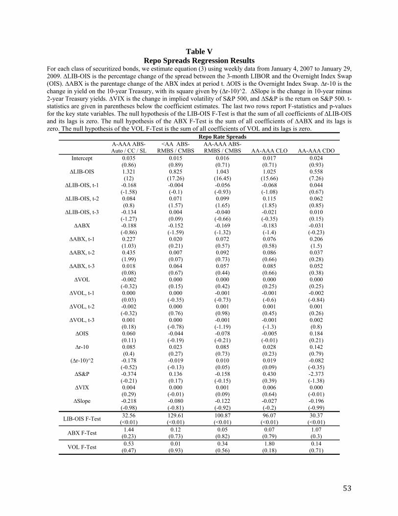
  53

Table V  Repo Spreads Regression Results

For each class of securitized bonds, we estimate equation (3) using weekly data from January 4, 2007 to January 29, 2009. ∆LIB-OIS is the percentage change of the spread between the 3-month LIBOR and the Overnight Index Swap (OIS). ∆ABX is the parentage change of the ABX index at period t. ∆OIS is the Overnight Index Swap. ∆r-10 is the change in yield on the 10-year Treasury, with its square given by (∆r-10)^2. ∆Slope is the change in 10-year minus 2-year Treasury yields. ∆VIX is the change in implied volatility of S&P 500, and ∆S&P is the return on S&P 500. t-statistics are given in parentheses below the coefficient estimates. The last two rows report F-statistics and p-values for the key state variables. The null hypothesis of the LIB-OIS F-Test is that the sum of all coefficients of ∆LIB-OIS and its lags is zero. The null hypothesis of the ABX F-Test is the sum of all coefficients of ∆ABX and its lags is zero. The null hypothesis of the VOL F-Test is the sum of all coefficients of VOL and its lags is zero.

Repo Rate Spreads

A-AAA ABS-Auto / CC / SL

<AA ABS-RMBS / CMBS

AA-AAA ABS-RMBS / CMBS AA-AAA CLO AA-AAA CDO

Intercept 0.035 0.015 0.016 0.017 0.024 (0.86) (0.89) (0.71) (0.71) (0.93)

∆LIB-OIS 1.321 0.825 1.043 1.025 0.558 (12) (17.26) (16.45) (15.66) (7.26)

∆LIB-OIS, t-1 -0.168 -0.004 -0.056 -0.068 0.044 (-1.58) (-0.1) (-0.93) (-1.08) (0.67)

∆LIB-OIS, t-2 0.084 0.071 0.099 0.115 0.062 (0.8) (1.57) (1.65) (1.85) (0.85)

∆LIB-OIS, t-3 -0.134 0.004 -0.040 -0.021 0.010 (-1.27) (0.09) (-0.66) (-0.35) (0.15)

∆ABX -0.188 -0.152 -0.169 -0.183 -0.031 (-0.86) (-1.59) (-1.32) (-1.4) (-0.23)

∆ABX, t-1 0.227 0.020 0.072 0.076 0.206 (1.03) (0.21) (0.57) (0.58) (1.5)

∆ABX, t-2 0.435 0.007 0.092 0.086 0.037 (1.99) (0.07) (0.73) (0.66) (0.28)

∆ABX, t-3 0.018 0.064 0.057 0.085 0.052 (0.08) (0.67) (0.44) (0.66) (0.38)

∆VOL -0.002 0.000 0.000 0.000 0.000 (-0.32) (0.15) (0.42) (0.25) (0.25)

∆VOL, t-1 0.000 0.000 -0.001 -0.001 -0.002 (0.03) (-0.35) (-0.73) (-0.6) (-0.84)

∆VOL, t-2 -0.002 0.000 0.001 0.001 0.001 (-0.32) (0.76) (0.98) (0.45) (0.26)

∆VOL, t-3 0.001 0.000 -0.001 -0.001 0.002 (0.18) (-0.78) (-1.19) (-1.3) (0.8)

∆OIS 0.060 -0.044 -0.078 -0.005 0.184 (0.11) (-0.19) (-0.21) (-0.01) (0.21)

∆r-10 0.085 0.023 0.085 0.028 0.142 (0.4) (0.27) (0.73) (0.23) (0.79)

(∆r-10)^2 -0.178 -0.019 0.010 0.019 -0.082 (-0.52) (-0.13) (0.05) (0.09) (-0.35)

∆S&P -0.374 0.136 -0.158 0.430 -2.373 (-0.21) (0.17) (-0.15) (0.39) (-1.38)

∆VIX 0.004 0.000 0.001 0.006 0.000 (0.29) (-0.01) (0.09) (0.64) (-0.01)

∆Slope -0.218 -0.080 -0.122 -0.027 -0.196 (-0.98) (-0.81) (-0.92) (-0.2) (-0.99)

LIB-OIS F-Test 32.56 129.61 100.87 96.07 30.37 (<0.01) (<0.01) (<0.01) (<0.01) (<0.01)

ABX F-Test 1.44 0.12 0.05 0.07 1.07 (0.23) (0.73) (0.82) (0.79) (0.3)

VOL F-Test 0.53 0.01 0.34 1.80 0.14 (0.47) (0.93) (0.56) (0.18) (0.71)

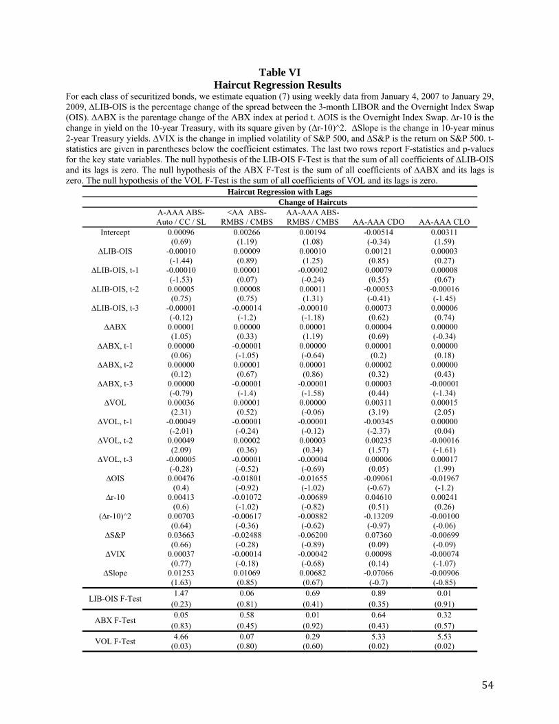
  54

Table VI Haircut Regression Results

For each class of securitized bonds, we estimate equation (7) using weekly data from January 4, 2007 to January 29, 2009, ∆LIB-OIS is the percentage change of the spread between the 3-month LIBOR and the Overnight Index Swap (OIS). ∆ABX is the parentage change of the ABX index at period t. ∆OIS is the Overnight Index Swap. ∆r-10 is the change in yield on the 10-year Treasury, with its square given by (∆r-10)^2. ∆Slope is the change in 10-year minus 2-year Treasury yields. ∆VIX is the change in implied volatility of S&P 500, and ∆S&P is the return on S&P 500. t-statistics are given in parentheses below the coefficient estimates. The last two rows report F-statistics and p-values for the key state variables. The null hypothesis of the LIB-OIS F-Test is that the sum of all coefficients of ∆LIB-OIS and its lags is zero. The null hypothesis of the ABX F-Test is the sum of all coefficients of ∆ABX and its lags is zero. The null hypothesis of the VOL F-Test is the sum of all coefficients of VOL and its lags is zero.

Haircut Regression with Lags Change of Haircuts

A-AAA ABS-Auto / CC / SL

<AA ABS-RMBS / CMBS

AA-AAA ABS-RMBS / CMBS AA-AAA CDO AA-AAA CLO

Intercept 0.00096 0.00266 0.00194 -0.00514 0.00311 (0.69) (1.19) (1.08) (-0.34) (1.59)

∆LIB-OIS -0.00010 0.00009 0.00010 0.00121 0.00003 (-1.44) (0.89) (1.25) (0.85) (0.27)

∆LIB-OIS, t-1 -0.00010 0.00001 -0.00002 0.00079 0.00008 (-1.53) (0.07) (-0.24) (0.55) (0.67)

∆LIB-OIS, t-2 0.00005 0.00008 0.00011 -0.00053 -0.00016 (0.75) (0.75) (1.31) (-0.41) (-1.45)

∆LIB-OIS, t-3 -0.00001 -0.00014 -0.00010 0.00073 0.00006 (-0.12) (-1.2) (-1.18) (0.62) (0.74)

∆ABX 0.00001 0.00000 0.00001 0.00004 0.00000 (1.05) (0.33) (1.19) (0.69) (-0.34)

∆ABX, t-1 0.00000 -0.00001 0.00000 0.00001 0.00000 (0.06) (-1.05) (-0.64) (0.2) (0.18)

∆ABX, t-2 0.00000 0.00001 0.00001 0.00002 0.00000 (0.12) (0.67) (0.86) (0.32) (0.43)

∆ABX, t-3 0.00000 -0.00001 -0.00001 0.00003 -0.00001 (-0.79) (-1.4) (-1.58) (0.44) (-1.34)

∆VOL 0.00036 0.00001 0.00000 0.00311 0.00015 (2.31) (0.52) (-0.06) (3.19) (2.05)

∆VOL, t-1 -0.00049 -0.00001 -0.00001 -0.00345 0.00000 (-2.01) (-0.24) (-0.12) (-2.37) (0.04)

∆VOL, t-2 0.00049 0.00002 0.00003 0.00235 -0.00016 (2.09) (0.36) (0.34) (1.57) (-1.61)

∆VOL, t-3 -0.00005 -0.00001 -0.00004 0.00006 0.00017 (-0.28) (-0.52) (-0.69) (0.05) (1.99)

∆OIS 0.00476 -0.01801 -0.01655 -0.09061 -0.01967 (0.4) (-0.92) (-1.02) (-0.67) (-1.2)

∆r-10 0.00413 -0.01072 -0.00689 0.04610 0.00241 (0.6) (-1.02) (-0.82) (0.51) (0.26)

(∆r-10)^2 0.00703 -0.00617 -0.00882 -0.13209 -0.00100 (0.64) (-0.36) (-0.62) (-0.97) (-0.06)

∆S&P 0.03663 -0.02488 -0.06200 0.07360 -0.00699 (0.66) (-0.28) (-0.89) (0.09) (-0.09)

∆VIX 0.00037 -0.00014 -0.00042 0.00098 -0.00074 (0.77) (-0.18) (-0.68) (0.14) (-1.07)

∆Slope 0.01253 0.01069 0.00682 -0.07066 -0.00906 (1.63) (0.85) (0.67) (-0.7) (-0.85)

LIB-OIS F-Test 1.47 0.06 0.69 0.89 0.01

(0.23) (0.81) (0.41) (0.35) (0.91)

ABX F-Test 0.05 0.58 0.01 0.64 0.32

(0.83) (0.45) (0.92) (0.43) (0.57)

VOL F-Test 4.66 0.07 0.29 5.33 5.53 (0.03) (0.80) (0.60) (0.02) (0.02)

  55