Int J Comput Vis manuscript No.(will be inserted by the editor)

RSLAM: A System for Large-Scale Mapping inConstant-Time using Stereo

Christopher Mei · Gabe Sibley · Mark Cummins · Paul Newman · Ian

Reid

Received: date / Accepted: date

Abstract Large scale exploration of the environmentrequires a constant time estimation engine. Bundle ad-

justment or pose relaxation do not fulfil these require-

ments as the number of parameters to solve grows withthe size of the environment. We describe a relative si-

multaneous localisation and mapping system (RSLAM)

for the constant-time estimation of structure and mo-tion using a binocular stereo camera system as the sole

sensor. Achieving robustness in the presence of difficult

and changing lighting conditions and rapid motion re-

quires careful engineering of the visual processing, andwe describe a number of innovations which we show lead

to high accuracy and robustness. In order to achieve

real-time performance without placing severe limits onthe size of the map that can be built, we use a topo-

metric representation in terms of a sequence of relative

locations. When combined with fast and reliable loop-closing, we mitigate the drift to obtain highly accurate

global position estimates without any global minimisa-

tion. We discuss some of the issues that arise from us-

ing a relative representation, and evaluate our systemon long sequences processed at a constant 30-45 Hz, ob-

taining precisions down to a few meters over distances

of a few kilometres.

Keywords SLAM · Stereo · Tracking · Loop Closing ·SIFT

1 Introduction

Building autonomous platforms using vision sensors has

encouraged many developments in low-level image pro-

C. Mei, G. Sibley, M. Cummins, P. Newman and I. Reid

Robotics Research Group, Department of Engineering Science,Parks Road, Oxford, OX1 3PJ

E-mail: {cmei,gsibley,mjc,pnewman,ian}@robots.ox.ac.uk

cessing and in estimation techniques. Recent improve-ments have lead to real-time solutions on standard hard-

ware. However these often rely on global solutions that

do not scale with the size of environment. Further-more, few systems integrate loop closure or a relocali-

sation mechanism that is essential for working in non-

controlled environments where tracking assumptions areoften violated. In this work, we investigate how to effi-

ciently combine relevant approaches to obtain a vision-

based solution that provides high frame rate, constant-

time exploration, resilience to motion blur and a relo-cation and loop closure mechanism.

Vision-based systems can be classified between monoc-ular and stereo solutions. The presence of a single cam-

era on an increasing amount of consumer goods (mo-

bile phones, personal digital assistants, laptops, etc.) is

a strong motivation for research in monocular vision.However the use of a monocular system can lead to

failure modes due to non-observability (e.g. with pure

rotation), problems with scale propagation and requiresextra computation to provide depth estimates. To avoid

these issues, the current system uses a stereo pair which

paradoxically reduces the computation as low-level pro-cessing can take advantage of scale (Section 6) and rely

less on expensive joint depth and pose estimation.

The relative SLAM system presented in this papercombines a world representation enabling loop closure

in real-time (Section 3) with carefully engineered low-

level image processing adapted to stereo image pairs.The novelty in the world representation comes from the

continuous relative formulation that avoids map merg-

ing and the transfer of statistics between sub-maps.

We describe a scheme for relative bundle adjustment(RBA) within this framework that leads to improved

precision in Section G. In this article, we demonstrate

the integration of three key components: (i) a represen-

2

tation of the global environment in terms of a continu-

ous sequence of relative locations; (ii) a visual process-ing front-end that tracks features with sub-pixel accu-

racy, computes temporal and spatial correspondences,

and estimates precise local structure from these fea-tures; (iii) a method for loop-closure which is indepen-

dent of the map geometry, and solves the loop closure

and kidnapped robot problem; to produce a system ca-pable of mapping long sequences over large distances

with high precision, but in constant time.

The remainder of the article is structured as fol-lows. After a section on related work, we discuss the

representation of the environment chosen in this work

and how it relates to standard methods in computervision and robotics. In Section 6 we investigate the no-

tion of “true scale” or how a stereo pair can provide

an efficient approach to generating scale-invariant de-scriptors. Section 4 then describes the different visual

processing steps to estimate the position of the cam-

era and build the map from the stereo images. Section

5 addresses the problems of relocalisation (i.e. how torecover when tracking fails) and loop closure (i.e. how

to recognise a previously mapped region). Finally, we

analyse the performance of the system on simulated andlarge-scale indoor and outdoor sequences.

2 Related work

In this section, we will discuss specifically recent ad-

vances in visual SLAM (Simultaneous Localisation and

Mapping) with a focus on stereo systems. A broadersurvey of SLAM approaches can be found for exam-

ple in (Thrun et al (2005); Durrant-Whyte and Bailey

(2006); Bailey and Durrant-Whyte (2006)).

Visual SLAM has seen many successful systems in

recent years. Several approaches have been proposedfor estimating the motion of a single camera and the

structure of the scene in real-time. The application of an

Extended Kalman Filter (EKF) to this problem yielded

one of the earlier real-time monocular SLAM systems(Davison (2003); Davison et al (2007)). However the

EKF suffers from a number of problems which have

proven limiting:

– the number of landmarks that can be processed islimited to a few hundred due to quadratic complex-

ity of the EKF. Bundle adjustment (Triggs et al

(1999)) has a complexity linear in the number of

landmarks (but cubic in the number of poses) en-abling the processing of more landmarks.

– consistency. EKF is known to produce inconsistent

estimates (Julier and Uhlmann (2001)), one of the

weaknesses being the impossibility of relinearising

the cost function after marginalisation.

These reasons have lead recent real-time monocular

systems to use local (Mouragnon et al (2006)) or global(Klein and Murray (2007); Eade and Drummond (2007,

2008)) bundle adjustment as the underlying estimator.

A careful choice of key-frames is however required to

keep the solving tractable. Compared to our presentwork, (Mouragnon et al (2006)) does not provide a

loop closing mechanism and cannot as such reduce drift

when returning to a previously explored region. (Kleinand Murray (2007)) is a system aimed at small environ-

ments with applications in augmented reality. It uses

a separate thread for bundle adjustment enabling thebuilding of accurate maps but is not adapted to large

scale exploration. (Eade and Drummond (2007, 2008))

share strong similarities with the present work com-

bining a relative representation and a non-probabilisticloop closure mechanism. In this work however, the low-

level image processing is adapted to stereo vision and

the focus is on precise exploration without global graphminimisation.

Recent research has also provided some real-time

solutions using stereo pairs (Nister et al (2006); Kono-

lige and Agrawal (2008)). In (Nister et al (2006)), theauthors rely on local bundle adjustment using a global

representation but do not address the problem of loop

closing. The closest related work is the FrameSLAMsystem by Konolige and Agrawal (Konolige and Agrawal

(2008)). FrameSLAM and the current system differ mainly

in the objective: FrameSLAM focuses on reducing the

complexity of large-scale solving whereas we aim atproviding a locally accurate map and trajectory using

relative bundle adjustment with a bounded complex-

ity (Section G). As such, the complexity of FrameS-LAM grows with the size of the environment (albeit

slowly) whereas the current approach is constant-time.

For many applications (path planning, object manipu-lation, dynamic object detection, ...) good local accu-

racy is sufficient and we show that it can be recovered in

constant time (the complexity being related to the size

of the working space). It is also important to note thatglobal metric maps and relative maps are not equivalent

(see Section 3.2) and share different properties.

3 Map representation

In this section, we introduce our Continuous RelativeRepresentation (CRR), used to represent the location

of map features with respect to the current sensor posi-

tion. Since it differs in subtle but important ways from

3

the prior art, we begin with a review of representations

that have been used previously with some success.

3.1 World representations

The position of the robot and the landmarks repre-

senting the environment can be represented in different

ways (Fig. 1):

Global coordinates. (Fig. 1(a)) The most com-

mon representation is to a fix an arbitrary initial

frame (usually set to be the identity transform) and

represent all subsequent position and landmark es-timates with respect to this frame.

Robo-centric coordinates. (Fig. 1(b)) This is sim-

ilar to using global coordinates but the initial frameis chosen to be the current robot position. The map

has to be updated at each new position estimate.

This representation has been shown to improve con-sistency for EKF SLAM estimation (Castellanos et al

(2004)).

Relative representation. (Bosse et al (2004); Eade

and Drummond (2008); Konolige and Agrawal (2008);Moore et al (2009)). (Fig. 1(d),1(e)) In this frame-

work, each camera position is connected by an edge

transform to another position forming a graph struc-ture. There is no privileged position and recovering

landmark estimates requires a graph traversal (e.g.

breadth first search or shortest path computation).

Sub-maps. (Fig. 1(c), 1(d)) Sub-maps consist in

representing a map by local frames and can be used

with any of the previously discussed map represen-tations. There are mainly two reasons for using sub-

maps: reducing the computation and improving the

consistency (mainly in filtering frameworks to re-

duce the effect of propagating inconsistent statis-tics).

In the presented system, the robot position and map

are represented in a continuous relative framework (CRR)(Fig. 1(e)).

Several related methods have been described in the

literature. In the recent work by Moore et al (Mooreet al (2009)), the authors provide a representation sim-

ilar to a CRR without graph exploration. The authors

do not address the problem of refining local estimatesand do not discuss loop closure. The representation is

used to fuse global low-frequency measurements (e.g.

GPS at 1Hz) with high frequency local estimates (pro-

vided for example by an inertial measurement unit at100Hz). Compared to the present approach, this work

is aimed at providing stable motion estimates for robot

navigation and the focus is less on the mapping aspect

of the problem. In the works by Bosse et al (Bosse et al

(2004)) and Eade and Drummond (Eade and Drum-mond (2008)) information is fused locally into sub-maps

that are connected by relative transforms as in Fig.

1(d). Fusing information leads to a number of difficul-ties: (i) map-merging is required at loop closure (Bosse

et al (2004)) (ii) computing a global solution can be-

come expensive due to the locally dense covariance struc-tures produced by marginalisation and (iii) it is no

longer possible to benefit from better precision and con-

sistency by relinearisation. Furthermore, as explained

in the following section, choosing what information tomerge can be hard and have a strong impact on the final

results. In contrast, relative bundle adjustment (Section

G) using a CRR framework has the advantages of stan-dard bundle adjustment (a sparse Hessian structure and

the possibility of relinearising) and does not require a

complex map-merging step at loop closure. This rep-resentation can be seen as the limit of a sub-mapping

approach when the size of the local map is reduced to

containing a single frame.

3.2 Continuous Relative Representation (CRR)

Terminology The following terms are used to describe

different aspects of the CRR:

– a base frame is defined as the pose in which a land-

mark is represented (i.e. where its 3-D coordinatesare kept),

– an active region corresponds to the set of poses

within a given distance in the graph to the currentpose.

A continuous relative representation (CRR) was cho-

sen to represent the world as described in Fig. 2. During

the exploration of the environment, each new pose ofthe robot becomes a vertex in a graph connected by

an edge representing the estimated transform between

poses. In Fig. 2, this edge is indicated by a continuous

line. The active region contains the set of poses withina given distance in the graph to the current pose. In

the example, an active region of size two was chosen.

Generally, the active region will be comprised of thelatest poses. However, in the case of a loop closure, as

illustrated by Fig. 2(b), older poses will also form the

active region.The active region defines the landmarks visible from

the current frame. Representing the local environment

around the robot consists in projecting the active region

into the current frame. Landmarks with base frames(where the landmark’s 3-D coordinates are kept) be-

longing to poses from the active region are projected

into the current frame by composing the transforms

4

(a) Global (b) Robo-centric

(c) Global Sub-mapping (d) Relative Sub-mapping (e) Continuous relative representation (CRR)

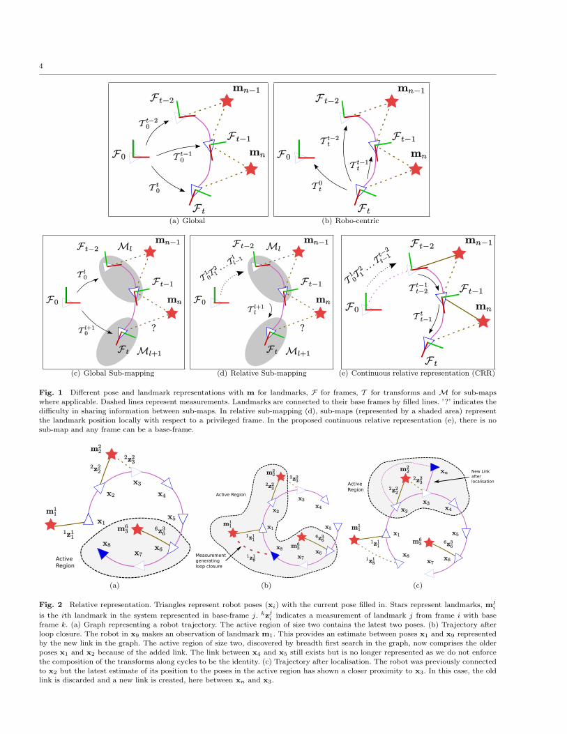
Fig. 1 Different pose and landmark representations with m for landmarks, F for frames, T for transforms and M for sub-mapswhere applicable. Dashed lines represent measurements. Landmarks are connected to their base frames by filled lines. ’?’ indicates the

difficulty in sharing information between sub-maps. In relative sub-mapping (d), sub-maps (represented by a shaded area) representthe landmark position locally with respect to a privileged frame. In the proposed continuous relative representation (e), there is nosub-map and any frame can be a base-frame.

(a) (b) (c)

Fig. 2 Relative representation. Triangles represent robot poses (xi) with the current pose filled in. Stars represent landmarks, mji

is the ith landmark in the system represented in base-frame j. kzji indicates a measurement of landmark j from frame i with base

frame k. (a) Graph representing a robot trajectory. The active region of size two contains the latest two poses. (b) Trajectory afterloop closure. The robot in x9 makes an observation of landmark m1. This provides an estimate between poses x1 and x9 representedby the new link in the graph. The active region of size two, discovered by breadth first search in the graph, now comprises the olderposes x1 and x2 because of the added link. The link between x4 and x5 still exists but is no longer represented as we do not enforce

the composition of the transforms along cycles to be the identity. (c) Trajectory after localisation. The robot was previously connectedto x2 but the latest estimate of its position to the poses in the active region has shown a closer proximity to x3. In this case, the oldlink is discarded and a new link is created, here between xn and x3.

5

along the edges. For example, in Fig. 2(a), projecting

landmark m3 (the upper script is used here to indicatethat it is represented in frame 6) in the current frame

will require to compose through x7: m83 = T 7

8 T 67 m6

3. In

this work, the discovery of the active region is made bya breadth first search (BFS). A probabilistic approach

could also be used with a Dijkstra shortest path discov-

ery using the covariance from the edge transformations,but previous research has shown a negligible improve-

ment over the map quality (Bosse et al (2004)).

The projected estimates (or local map) can be used

for obstacle avoidance, grasping or in this work to es-

tablish matches and compute the position of the robot.In the current setting we do not use the uncertainty

provided by the estimates for the data association but

use a fixed-size window. In this framework, loop clo-

sure consists in creating a new edge that can then beused to transfer 3-D landmark estimates into the cur-

rent frame and therefore evaluate their projection in

the image (Fig. 2(b)).

It should be noted that the global solution minimis-

ing the reprojection error in a relative framework is notequivalent to the global solution using a global refer-

ence with the same measurements. In the case of unob-

servable ego-motion (e.g. if the robot uses a means oftransport such as a lift or car), the map cannot be repre-

sented in a Euclidean setting. Methods that use a global

frame would fail but a relative representation still holds.This would also be the case when sub-mapping with a

local map that overlaps such regions. This observation

leads to a change in perspective where the importance

of detecting changes in the environment becomes ap-parent as imposing global constraints blindly (such as

those imposed in a pose relaxation framework) would

degrade the accuracy of the map.

3.3 Relative Bundle Adjustment (RBA)

Bundle adjustment computes the optimal (maximal like-

lihood function under the assumption of Gaussian un-

certainty) structure and motion from a set of corre-

sponding image projections. It is a well studied prob-lem in the context of a single global coordinate frame

(Triggs et al (1999)).

The cost function minimises the reprojection be-

tween landmark mi and its measurements zji in image j

for all Mi images and all N landmarks. Let Projj be theprojection of mi in image j. In a global frame, Projj

is a function of the position of frame j with respect to

the origin. Assuming the measurement zj is normally

distributed zji ∼ N (Projj(mi), Σi,j), we obtain:

F =

N∑

i=1

Mi∑

j=1

(zi − Projj(mi))⊤Σ−1

i,j (zi − Projj(mi))

The computation of the reprojection error in a CRR

framework differs from the computation in a global co-ordinate frame as each landmark estimate requires the

traversal of the graph along the kinematic chains link-

ing the base-frame to the images observing the land-

mark. (This traversal corresponds to the computationof a metric on the manifold defined by the trajectory

frames in the graph.)

In other words, in this context, the projection func-

tion Projj now also depends on the base-frame k oflandmark mk

j and thus on all the transforms linking

the two frames:

Projj,k = f(T jk ) = f(T k−1

k , T k−2k−1 , . . . , T j+1

j+2 , T jj+1)

As with standard bundle adjustment, this problem

is solved using Gauss-Newton minimisation. As discussed

in the previous section, this cost function has a differentminimum to the standard approach. Furthermore the

sparsity pattern is changed. However sparsity remains

which is key to solving the problem in real-time. In (Sib-ley et al (2009)), we consider in much greater detail the

implications of the CRR and RBA. In particular, we

present empirical evidence that strongly suggests thisremains a constant-time algorithm.

4 Stereo visual processing

This section describes the different steps applied to pro-

cessing stereo image pairs. It is similar to other works

in the literature (Nister et al (2006); Klein and Murray(2007)), the main novelty is in: a) the systematic ap-

plication of second-order minimisation (Benhimane and

Malis (2004); Mei et al (2008)) for the pose initialisa-tion and sub-pixel refinement, b) the use of quadtrees to

ensure adequate spreading of the features in the image

and c) the use of true scale (Section 6) to build discrim-

inative descriptors at a lower cost than the standardscale-space computation combined with a descriptor (as

in SIFT (Lowe (2004))).

We begin with a top level view. For each incoming

frame, the following steps are made:

A image pre-processing,

B feature extraction,

C pose initialisation through sum-of-squared difference(SSD) inter-frame tracking,

D temporal feature matching: the features are matched

with current 3-D landmark estimates (the map),

6

E localisation: the position of the camera pair is esti-

mated by minimising the landmark to image repro-jection error,

F left-right matching: new 3-D landmarks are initialised

by matching image templates between the left andright images along scanlines and triangulating the

results.

G relative bundle adjustment.

We will discuss in detail the different processingsteps.

A Image pre-processing

Each incoming image is rectified using the known cam-

era calibration parameters to ensure efficient scanlinesearches of corresponding left-right matches (Hartley

and Zisserman (2000)). The image intensities for left

and right images are then corrected to obtain the samemean and variance. This step improves the left-right

matching scores, enabling better detection of outliers.

A scale-space pyramid of both images is then built us-

ing a box filter with one image per octave for compu-tational efficiency. Using a pyramid yields features at

different scales, giving greater resilience to focus and

motion blur. It is also used for the pose initialisationand the calculation of SIFT descriptors.

B Feature extraction

The feature locations used in this work are provided

by the FAST corner extractor (Rosten and Drummond(2005)) that provides good repeatability at a small com-

putational cost. To obtain resilience to blur and enable

matching over larger regions in the image, FAST cor-

ners are extracted at different levels of the scale-spacecomputed in the previous step. In practise, we used

three pyramid levels in processing indoor sequences,

but found that two levels were sufficient for our out-door sequences; the type of camera, and the amount of

motion blur expected are factors which influence this

parameter.

The corner extraction threshold is initially set at

a value providing a compromise between number of

points and robustness to noise. This threshold is then

decreased or increased at each time-step to ensure aminimal number of points. This proved sufficient to

adapt to the strong changes in illumination and low

contrast typically encountered in outdoor sequences.

C Pose initialisation with image-based gradient

descent

The apparent image motion of features in visual SLAM

is typically dominated by the ego-rotation, and largeinter-frame rotation is a common failure mode for sys-

tems based on an inter-frame feature search. To improve

robustness, an estimate of the 3-D rotation is obtainedusing the algorithm described in (Mei et al (2008)) at

the highest level of the scale-space pyramid for effi-

ciency and to widen the basin of convergence. This algo-rithm minimises the sum-of-squared-distance of image

intensity using a second-order gradient descent minimi-

sation (ESM). The obtained estimate is then used to

guide the search for temporal feature correspondences.The complexity of the tracking algorithm is O(p2n)

with p the number of parameters (p = 3 for a rota-

tion) and n the number of pixels. The following timingsfor one iteration were obtained for the architecture de-

scribed in Section 7.5:

32 × 24 64 × 48 128 × 96

0.16ms 0.58ms 2.16ms

On average, 4 iterations were required to converge. Inthe tested sequences an image of size 32 × 24 was used

for tracking.

D Temporal feature matching

The current 6-DOF pose is initialised to the rotation

computed in the previous stage, and a translation of

zero relative to the previous pose. The 3-D coordinatesof the landmarks (i.e. the map) computed through the

graph representing the relative poses (as detailed in

Section 3.2) are then projected into the left and rightimages of the current stereo pair and matched in a

fixed-sized window to the extracted FAST corners using

mean SAD (sum of absolute difference with the meanremoved for better resilience to lighting changes) on im-

age patches of size 9×9. This step is then followed by

image sub-pixel refinement using ESM. Matches whose

score fall below a threshold after ESM are rejected. Ap-plying this threshold after sub-pixel refinement provides

a more meaningful comparison as patches with high fre-

quency will typically have high errors before the sub-pixel refinement. The influence of sub-pixel refinement

over the accuracy of the motion estimates will be eval-

uated in Section 7.

E Localisation

After the map points have been matched, 3-point pose

RANSAC (Fischler and Bolles (1981); Nister et al (2006))

7

is applied to obtain an initial pose estimate and out-

lier classification. The total reprojection error over bothviews is then minimised using m-estimators for robust-

ness (this minimisation can be found in standard text-

books (Hartley and Zisserman (2000))). After the min-imisation, landmark measurements with strong repro-

jection errors are removed from the system. This step

proved important to enable early removal of outliersand the possibility of adding new, more stable, land-

marks.

F Initialising new features

To achieve good accuracy at a high frame-rate we aim

to measure between 100-150 features, with a fairly even

spatial distribution across the image, at every time-

step. Thus after temporal matches have been estab-lished we seek to initialise new features in the current

frame. The feature selection process uses quadtrees, de-

scribed in following subsection, to ensure a uniform dis-tribution of the features. Information theory could also

be used to select features that constrain the motion es-

timation and for setting the search region for tracking(Chli and Davison (2008)) but the quadtree approach

proved sufficient in the tested sequences.

Along with each feature track, an image patch (ofsize 9×9) is saved for sub-pixel matching in time and

a SIFT descriptor is computed for robust relocalisation

and loop closure (Section 5).

Feature selection using quadtrees

The feature selection process follows the assumptionthat we desire distinctive features with a uniform dis-

tribution in the image (irrespective of the underlying

tracking uncertainty). A quadtree is used to representthe distribution of the measurements at each time step.

It contains the number of measurements in the different

parts of the image and the maximal amount of pointsallowed, to ensure a uniform distribution of features. It

is used in the following way:

1. In Step D., the matched map points increment thequadtree count according to their measurement im-

age locations.

2. To add new features, FAST corners are extractedfrom the left and right images and ordered by a

distinctiveness score (in this work we used Harris

scores). To decide which features to add, the best

features are taken in order and their image locationis checked in the quadtree to ensure the maximal

amount of allowed points has not been exceeded.

If it passes the test, a match is sought along the

corresponding epipolar line (scan-line). This search

begins by looking for a suitable FAST corner on thisline. However if this fails, we perform a dense SAD

search, seeking the patch along the scan-line that

correlates best with the feature patch. Although slower,this enables us to initialise features where FAST has

fired only in one of the images. This allows us to put

features in areas that provide good constraints formotion estimation although the corner response is

weak. The precision of final match is then improved

by sub-pixel second-order minimisation (Benhimane

and Malis (2004)) over the image coordinates andthe average intensity (three parameter minimisa-

tion).

G Relative bundle adjustment

The final step to improve the local estimates is to ap-

ply relative bundle adjustment. Near optimal parame-

ter estimates lead to longer feature tracks, resilience to

higher reprojection errors, less clutter and lower mem-ory usage. This final refinement step is important and

experimentally was shown to reduce errors by a fac-

tor of two. However it is not strictly necessary and thecurrent article focuses mainly on obtaining high-quality

initial estimates.

This is important because it indicates that our care-

ful low-level stereo image processing greatly reduces the

computational burden (and to a certain extent the re-

quirement) of full bundle adjustment. (This is of partic-ular interest for platforms with limited computational

resources such as phones.)

5 Relocalisation and loop closure

The method described above is generally successful in

the normal course of operation. Nevertheless failures

are almost inevitable, and there is a need for more re-

silient methods that enable the system to recover (i.e.relocalise) after such failures, as well to detect a re-

turn to previously mapped areas (i.e. loop closure). For

both processes we make use of the SIFT descriptorscomputed on feature initialisation.

5.1 Relocalisation

The system uses a standard relocalisation mechanism

when data association fails between consecutive frames.The “true scale” SIFT descriptors (Section 6) between

the current and the previous frames are matched by di-

rect comparison. 3-point-pose RANSAC (Fischler and

8

Bolles (1981)) is then applied to robustly find the pose

of the platform. If this step fails, loop closure (Sec-tion 5.2) is attempted on subsequent frames. This ap-

proach takes advantage of the stereo setting and avoids

the training and memory requirement of methods suchas randomised trees (Lepetit and Fua (2006); Williams

et al (2007)).

5.2 Loop closure

For loop closure we rely on fast appearance based map-

ping (Cummins and Newman (2008))1. This approach

represents each place using the bag-of-words model de-veloped for image retrieval systems in the computer

vision community (Sivic and Zisserman (2003); Nister

and Stewenius (2006)). At time k the appearance mapconsists of a set of nk discrete locations, each location

being described by a distribution over which appear-

ance words are likely to be observed there. Incoming

sensory data is converted into a bag-of-words represen-tation; for each location, a query is made that returns

how likely it is that the observation came from that lo-

cation’s distribution or from a new place. This allowsus to determine if we are revisiting previously visited

locations.

FABMAP also returns possible feature matches thatcan be treated as normal matches in our visual process-

ing pipeline. More specifically, we apply the robust lo-

calisation described in Section 4. E. and, if successful,

we add a link in the graph containing this new esti-mate as in Fig. 2(b). The previous part of the map

will then be automatically discovered by BFS and used

for matching and localisation. This is how drift can bereduced through loop closure without requiring global

estimation.

In a filtering framework, incorrect loop closures areoften catastrophic as the statistical estimates are cor-

rupted. Using the CRR representation, an incorrect loop

closure would translate into attempting data associa-tion with landmarks from another part of the map. This

could be detected as the robust estimator would reject

most of the matches and a large proportion of tracked

landmarks would be newly initialised landmarks. Oncedetected, the CRR enables recovery from erroneous loop

closures as removing the incorrect graph link and bad

measurements returns the system to its previous state.

1 A version of FABMAP is available at www.robots.ox.ac.uk/

~mobile

5.3 Key frames and localisation

When exploring environments over long periods of time,

memory usage becomes an issue. The presented sys-tem uses a simple heuristic similar to that presented

in (Mouragnon et al (2006)) to decide what frames to

keep. Furthermore, when exploring a previously mapped

area detected by loop closure, the system localises withrespect to the active region thus reducing the amount

of new features created and simultaneously reducing

drift (Fig. 2(c) illustrates this mechanism). The met-ric for deciding when to connect poses is based on the

distance (typically 1 m) and angle (10 deg) between

frames and a minimum number of tracked landmarks(typically 50%).

6 True Scale

The well-known SIFT (Lowe (2004)) descriptor is built

at a scale determined by finding an extremum in scale

in a Difference of Gaussians (DoG) pyramid. The mostexpensive part of the algorithm is generally the compu-

tation of the image scale space. It has been shown to

be feasible in real-time (Eade and Drummond (2008))(without transferring the processing to a graphics card)

using a highly optimised recursive Gaussian filter and a

down-sampled image (320×240). In this work, we pro-

vide a different approach to scale invariance.

Previous work (Chekhlov et al (2007)) has also in-

vestigated solutions to avoid this cost in the case ofmonocular SLAM using the estimated camera pose. An

alternative is proposed here for stereo pairs that avoids

the knowledge of camera position. Landmark descrip-

tors are built corresponding to regions in the world ofsame physical size - we call this the “true scale” of the

feature. This provides the property of matching only

regions of same 3-D size which is not necessarily thecase with DoG features. It can be achieved at no extra

computational cost as the left-right matching that pro-

vides the 3-D location is required in any case for themotion estimation. True scale requires choosing a set of

3-D sizes for different depth ranges to ensure the pro-

jection size of the 3-D template lies within a given pixel

size range (Fig. 3).

We adopt a pinhole camera model with a focal length

f . The size in the image of the projection of a 3-D re-

gion of space is inversely proportional to its distance tothe centre of projection. Let smax and smin be the max-

imal and minimal size of square templates that could be

matched reliably. smax corresponds to a certain land-

9

(a) (b)

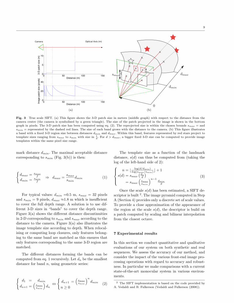
Fig. 3 True scale SIFT. (a) This figure shows the 3-D patch size in meters (middle graph) with respect to the distance from the

camera centre (the camera is symbolised by a green triangle). The size of the patch projected in the image is shown in the bottomgraph in pixels. The 3-D patch size has been computed using eq. (2). The reprojected size is within the chosen bounds smax = andsmin = represented by the dashed red lines. The size of each band grows with the distance to the camera. (b) This figure illustratesa band with a fixed 3-D region size between distances dmin and dmax. Within this band, features represented by red stars project to

template sizes ranging from smax to smin with size in 1

d. For d > dmax, a bigger fixed 3-D size can be computed to provide image

templates within the same pixel size range.

mark distance dmin. The maximal acceptable distance

corresponding to smin (Fig. 3(b)) is then:

{

dmax = smax

f

dmin = smin

f

⇒ dmax =smax

smindmin (1)

For typical values: dmin =0.5 m, smax = 32 pixels

and smin = 9 pixels, dmax ≈1.8 m which is insufficient

to cover the full depth range. A solution is to use dif-ferent 3-D sizes in “bands” to cover the depth range.

Figure 3(a) shows the different distance discontinuities

in 2-D corresponding to smin and smax according to thedistance to the camera. Figure 3(a) also illustrates the

image template size according to depth. When relocal-

ising or computing loop closures, only features belong-

ing to the same band are matched as this ensures thatonly features corresponding to the same 3-D region are

matched.

The different distances forming the bands can becomputed from eq. 1 recursively. Let dn be the smallest

distance for band n, using geometric series:

{

d1 = dmin

dn+1 =(

smax

smin

)

dn⇔

{

dn+1 =(

smax

smin

)n

dmin

n ≥ 0(2)

The template size as a function of the landmark

distance, s(d) can thus be computed from (taking the

log of the left-hand side of 2):

n = ⌊ log(d/dmin)log(smax/smin)⌋ + 1

s(d) = smax

(

dn

d

)

= smax

(

smax

smin

)n−1dmin

d

(3)

Once the scale s(d) has been estimated, a SIFT de-

scriptor is built 2. The image pyramid computed in StepA (Section 4) provides only a discrete set of scale values.

To provide a close approximation of the appearance of

the region at the scale s(d), the descriptor is build ona patch computed by scaling and bilinear interpolation

from the closest octave.

7 Experimental results

In this section we conduct quantitative and qualitativeevaluations of our system on both synthetic and real

sequences. We assess the accuracy of our method, and

consider the impact of the various front-end image pro-cessing operations with regard to accuracy and robust-

ness. In particular we make comparisons with a current

state-of-the-art monocular system in various environ-

ments.

2 The SIFT implementation is based on the code provided byA. Vedaldi and B. Fulkerson (Vedaldi and Fulkerson (2008)).

10

(a) Begbroke aerial view (b) New College aerial view

Fig. 4 Outdoor sequences.

Fig. 5 Image of the simulation setup

Video of our system running on both indoor and

outdoor sequences is available on the authors’ website.It exhibits the system’s behaviour in presence of mo-

tion blur, fog, lighting changes, lens flare and dynamic

objects.

7.1 Simulation

The simulation setup consists of 50 stereo frames gen-erated in a straight line and spaced every 20cm with

a 10cm baseline. Changes in illumination or automatic

camera intensity settings were simulated by adding aglobal intensity offset to all image values drawn from a

Gaussian distribution with a standard deviation of 15.

Sensor noise was simulated by adding random intensityvalues drawn independently from a Gaussian distribu-

tion with a standard deviation of 2.

In order to assess the accuracy of the system we

compare the pose estimate with ground truth and in-tegrate the (absolute) difference along the entire path

length. Note that this is different from simply compar-

ing the estimated end location against the ground truth

end location, since the latter may incorporate errors

which cancel, and also has the drawback that if the

system operates in a finite environment, the error isbounded by the size of the environment (consider a sys-

tem that simply travels in a small circle; its end-point

error will be bounded by the diameter of the circle).Figure 5 shows the final images of the sequence and the

estimated path.

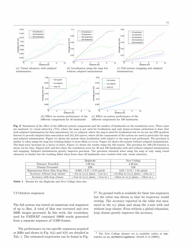
Figures 6(a)-6(e) show the precision obtained for

different numbers of landmarks and the effect of twodifferent aspects of the system: (a) data association us-

ing subpixel minimisation and (b) motion estimation

using the map and not only frame-to-frame tracking

(as in visual odometry). The results show that tracking100-150 landmarks with subpixel minimisation leads to

a precision of about 9cm per 100m or about one metre

per kilometre. This precision was also observed on realdata in good conditions (small amounts of blur and a

good feature distribution). Without subpixel minimisa-

tion, the error increased by a factor of three. This simu-lation combined with experiments on real data confirm

the importance of subpixel data association to obtain

precise estimates.

Visual odometry (VO) consists in removing step D

in Section 4 from the visual processing steps. We foundthat the precision was not reduced (and even appears

as slightly better towards the end because of the accu-

mulation of error in the 3-D landmark estimates withrespect to the latest pose). The good quality of VO

can be explained by the precise estimates from subpixel

minimisation but also the strong constraints provided

by the stereo pair (in contrast to a monocular system).One noticeable effect of not using the map was in the

robustness of the tracking. Tracking failure occurred

when fewer than 40 landmarks were used.

11

0 2 4 6 8 100

0.002

0.004

0.006

0.008

0.01

0.012

0.014

0.016

Distance (m)

Ave

rage

err

or (

m)

40 landmarks

100 landmarks

200 landmarks

(a) Visual odometry with subpixel

minimisation

0 2 4 6 8 100

0.02

0.04

0.06

0.08

0.1

Distance (m)

Ave

rage

err

or (

m)

20 landmarks

30 landmarks

100 landmarks

200 landmarks

(b) Localisation using the map but

without subpixel minimisation

0 2 4 6 8 100

0.01

0.02

0.03

0.04

0.05

Distance (m)

Ave

rage

err

or (

m)

10 landmarks

15 landmarks

30 landmarks

100 landmarks

200 landmarks

(c) Full system (mapping and subpixel

minimisation)

0 2 4 6 8 100

0.005

0.01

0.015

0.02

0.025

0.03

Distance (m)

Ave

rage

err

or (

m)

Full system

No subpixel

Only VO

(d) Effect on system performance of thedifferent components for 40 landmarks

0 2 4 6 8 100

0.005

0.01

0.015

0.02

0.025

0.03

Distance (m)

Ave

rage

err

or (

m)

Full system

No subpixel

Only VO

(e) Effect on system performance of thedifferent components for 100 landmarks

Fig. 6 Simulation of the effect of the different system components and the number of landmarks on the translation error. Three cases

are analysed: (i) visual odometry (VO), where the map is not used for localisation and only frame-to-frame estimation is done (butwith subpixel minimisation for data association) (ii) no subpixel, where the map is used for localisation but we do not use SSD gradientdescent to provide subpixel data association and (iii) full system, where all the components of the system are used in particular the map

and subpixel minimisation. Figure (a) shows the system when localisation with respect to the map is not performed. The precision issimilar to when using the map but tracking failure is more likely to occur. Figure (b) shows the system without subpixel minimisation.The final error increases by a factor of three. Figure (c) shows the results using the full system. The precision for 100-150 features isabout 1m for 1km. Figures 6(d) and 6(e) show the translation error for 40 and 100 landmarks with and without subpixel minimisation

and mapping. Subpixel minimisation greatly improves precision. The precision obtained when using the map or only using visualodometry is similar but the tracking failed when fewer than 40 landmarks were tracked with only visual odometry.

Begbroke New College

Distance Travelled 1.08 km 2.26 km

Frames Processed 23K 51K

Reprojection Error Min/Avg/Max 0.003 / 0.17 / 0.55 pixels 0.03 / 0.13 / 1.01 pixels

Accuracy without loop closure ∼1m in (x-y) plane, ∼1m in z ∼15-25m in (x-y) plane, ∼15m in z

Accuracy with loop closure ∼1cm in (x-y) plane, ∼1cm in z ∼10cm in (x-y) plane, ∼10cm in z

Table 1 Results for the Begbroke and New College data sets.

7.2 Outdoor sequences

The full system was tested on numerous real sequences

of up to 2km. A total of 5km was traversed and over300K images processed. In this work, the vocabulary

used for FABMAP contained 10000 words generated

from a separate sequence of 11200 frames.

The performance on two specific sequences acquired

at 20Hz and shown in Fig. 4(a) and 4(b) are detailed in

Tab. 1. The estimated trajectories can be found in Fig.

73. No ground truth is available for these two sequencesbut the robot was driven so that its trajectory would

overlap. The accuracy reported in the table was mea-

sured in the x-y plane and along the z-axis with andwithout loop closure. Even without a global relaxation,

loop closure greatly improves the accuracy.

3 The New College dataset set is available online at www.

robots.ox.ac.uk/NewCollegeData/ (Smith et al (2009)).

12

−40 −30 −20 −10 0 10−10

−5

0

5

10

15

20

25

30

35

x (m)

y (m

)

(a) Begbroke top view

−200

−150

−100

−50

0

50−50 0 50 100 150 200 250

x (m)

y (m)

(b) New College without loop closure

−140

−120

−100

−80

−60

−40

−20

0

20−50 0 50 100 150 200 250

y (m)

x (m

)

(c) New College top view with loop

closure

−30 −20 −10 0 10−100102030

−0.5

0

0.5

1

1.5

2

x (m)y (m)

z (m

)

(d) Begbroke side view

−200 −150 −100 −50 0 50

−200

0

200

400−5

0

5

10

15

x (m)y (m)

z (m

)

(e) New College side view without loop

closure

−200

−100

0

100

200

−100

0

100

200

300−20

0

20

x (m)y (m)

z (m

)(f) New College side view with loop closure

Fig. 7 Estimated trajectories for the data sets detailed in Tab. 1 containing three loops. The trajectories are shown processed withloop closure (red trajectory with crosses) and without (blue continuous line).

7.3 Indoor sequence

The system was tested on the “Atrium” indoor sequenceshown in Fig. 8(a). This short sequence acquired at

walking pace contains around 2K frames and was cho-

sen as: (a) it exhibits clear structure that provides a

visual indication of the quality of the estimates and (b)it is a challenging environment exhibiting regions with

little texture but also regions with repeated patterns.

Figure 8 shows two views of the estimated map andtrajectory. The alignment of the two staircases and the

structure of the floor is an indication of a good quality

estimate.

In this difficult setup, the stereo pair proved par-

ticularly useful as the data association provided by the

scanline search simplified the data association.

7.4 Robustness assessment and comparison to PTAM

In order to provide a qualitative assessment of the ben-

efits of our system, particularly the carefully engineeredvision front-end, we have compared it to a current state-

of-the-art monocular system, Parallel Tracking And Map-

ping (PTAM) (Klein and Murray (2007)) using the source

code available online4. This comparison highlights theimportance of the different processing steps proposed in

this article to provide robustness to varying conditions

in indoor and outdoor environments.

PTAM and the proposed system have different ob-jectives that have influenced the choice of the under-

lying algorithms. PTAM aims to provide a 3-D repre-

sentation of the world for augmented reality (AR) for

a small indoor workspace. RSLAM is aimed at bothindoor and outdoor applications that have lead us to

include mechanisms to deal with strong changes in il-

lumination and low contrast (Section 4.B) and providea good distribution of features in the image (Section

4.F). The choice of a stereo pair was also motivated by

the ease of map initialisation and in particular to avoidthe problem of unobservability common to all monocu-

lar systems; a pure rotation is a typical failure mode of

a monocular system since it provides no triangulation

baseline.

The PTAM system has a similar image process-

ing pipeline but requires a “bootstrapping” designed

to build an initial map that can be tracked and also

optimised using bundle adjustment in a background

4 PTAM can be downloaded at http://www.robots.ox.ac.uk/

~gk/PTAM/

13

(a) Atrium aerial view (b) Atrium side view (c) Atrium top view

Fig. 8 Atrium sequence. (a) shows a top view of the atrium and the trajectory taken (b) and (c) show the estimated trajectory and

map for the atrium indoor sequence. The structure of the steps are apparent. The first floor appears parallel to the ground and thestaircase are aligned indicating that the pose and map are correctly estimated.

thread. The initialisation phase requires a user to movethe camera to create a baseline. This phase is accept-

able for an AR application but is obviously a drawback

for applications such as robotics. A stereo system doesnot require this step as the baseline is known at the

start which greatly simplifies the initialisation of fea-

tures (Section 4.F).

PTAM was tested on the outdoor Begbroke sequence,the indoor Atrium sequence and in an office-like envi-

ronment. Different parameters of the PTAM software

were tested: distance between keyframes, coarse andfine search regions for data association during tracking,

rotation initialisation for coarse search and increasing

the computational time to allow better precision from

the bundle adjuster. The only parameter that improvedsignificantly the performance from the default values

was the distance between keyframes. This parameter

depends on the initial map scale generated from thebaseline during initialisation. This value is set to a sen-

sible value (10cm in the program) for AR but is not

adequate for outdoor sequences where the scales aredifferent.

We will start by describing the main difficulties en-

countered and will then describe which sequences in

particular were affected. The following three main dif-ficulties rendered the mapping particularly challenging

for the monocular system:

1. initialisation. It was difficult to find a sequence of

images that provided a good initialisation for the

system in the Begbroke and Atrium sequences. Forexample the motion at the start of the Begbroke

sequence is close to a pure rotation and few features

could be extracted on the ground.

2. poor feature distribution. As shown in Figure 9,imposing a good distribution of features is partic-

ularly important with images containing high fre-

quency produced for example from vegetation to

avoid poor trajectory estimates. PTAM does nothave such a mechanism which had a strong impact

not only at initialisation but also for subsequent

tracking. Figure 10(a) illustrates the features ex-tracted with a fixed threshold as in PTAM. Figure

10(e) shows the result obtained by RSLAM.

3. changes in illumination. In Section 4.B, a sim-ple mechanism was proposed to adapt the feature

extraction threshold to changes in illumination and

low contrast. PTAM does not provide such a method

and the tracking failed on sequences with low con-trast as in Fig. 10.

We did not test PTAM with loop closure. PTAM re-

quires precise global 3-D estimates to provide accurate

image reprojections for the tracking. At loop closure,this would be problematic as projecting previous parts

of the map requires a costly bundle adjustment that

is not real-time and grows cubicly with the number of

frames in the map. This is where a relative representa-tion would be beneficial.

The tests on the three sequences provided the fol-

lowing outcome:

1. Begbroke sequence. The Begbroke sequence proved

particularly challenging for the PTAM system. Onabout 80% of this sequence, the system failed due a

mixture between initialisation issues, poor feature

distributions or lack of features due to low con-trast. The longest continuous set of frames tracked

by PTAM is comprised of around 800 frames over a

distance of about 40m. On this part of the sequence,both systems provided a similar precision as shown

in Fig. 11(a) (the relative scale was estimated by

minimising the trajectory difference).

2. Indoor environment. In this experiment the cam-era used has a larger field of view (100 deg instead

of 65 deg), the ambient illumination did not change

greatly, and the distribution of features did not prove

14

(a) (b)

Fig. 9 Importance of quadtrees to provide a good feature distribution. These figures show the estimated trajectory for the Begbrokesequence using (a) the full system and (b) the system without quadtree feature selection. Taking the strongest Harris scores as inFig. (b) can lead to poorly constrained motion estimates. In the present case, the vegetation provides many strong Harris corners butleads to a poor feature distribution. Figure (a) illustrates that using a quadtree can provide a distribution of features that does notnecessary have the best Harris scores but provides strong constraints for motion estimation.

(a) Features extracted

with a standard thresholdon a low contrast image.

(b) Features extracted

with an automaticallyadapted threshold on alow contrast image.

(c) Best 100 features.

These features are similarirrespective of theextraction threshold.

(d) Extracted features

with constraineddistribution and astandard threshold.

(e) Extracted features

with constraineddistribution and anadapted threshold.

Fig. 10 Example of an image with low contrast in the Begbroke sequence (Fig. 4(a)). The tracking in PTAM failed as the featureextraction threshold is fixed and too high for this image as shown in Fig. 10(a). However simply reducing the threshold is not sufficient

as the features will suffer from a poor distribution as illustrated in Figures 10(b),10(c). It is by combining a mechanism to ensure agood distribution of features and a mechanism to adapt the threshold that it is possible to track in this situation Fig. 10(e).

critical. For these reasons PTAM is better suited to

this environment and consequently the results werebetter than for the outdoor sequence. Nevertheless

PTAM still exhibited a number of failures where

our system successfully tracked the entire sequence.

PTAM was able to track two separate sections (Fig.8): from the bottom of the atrium to the middle of

the first flight of stairs and from first floor to the

middle of the second staircase. The spatial aliasingcombined with low precision lead to incorrect data

association and tracking failure on the stairs (Fig.

11(b)). The estimated precision of the landmarkson the staircase was poor because of the small num-

ber of measurements and the small baseline.

3. Desktop environments. We also compared the

systems in a smallish desk and office space. Since

this is the environment for which PTAM was de-

signed, unsurprisingly it produced an accurate mapwith stable tracking. As reported in (Klein and Mur-

ray (2007)), the quality was improved when using

the larger field of view camera (100 deg instead of

65 deg). Our system was also able to build a goodquality map but close zoom-ins were not possible as

the system only initialises features that have left-

right correspondences (Section 4.F).

In conclusion, the empirical evidence of these experi-

ments points to the importance for robust camera track-

ing of careful engineering to compensate for changes in

lighting and of ensuring a good distribution of features.Our solution based on quadtrees is heuristic but effec-

tive. While these aspects could readily be incorporated

in a monocular system as well, we have also shown the

15

−5 0 5 10 15 20 25−15

−10

−5

0

(a) Comparison of the trajectories produces by PTAM and RSLAM on the longestcontinuous set of frames tracked by PTAM on the Begbroke sequence. It is

comprised of around 800 frames or about 40m. The trajectory estimated byPTAM is in blue with circles and the one estimated by RSLAM is in red withcrosses. The accuracy was similar for both systems.

(b) Stairs generated spatial aliasing in theAtrium sequence. This lead to failures intracking for the PTAM system. Using astereo pair increases the precision of themap, rendering the RSLAM system overallmore robust (although not immune) tospatial aliasing.

Fig. 11 Elements of comparison of PTAM and RSLAM on the Begbroke sequence (Fig. 8) and the Atrium sequence (Fig. 8(a)).

Times (ms) Min Avg Max

Pre-processing 7.6 11.9 29.8Tracking 1.4 3.8 10.0

RANSAC 0.1 0.3 3.4

Localisation 0.9 3.2 14.8Left-right matching 0.0 1.5 5.4SIFT descriptors 1.0 6.1 12.6

Total 15.3 26.8 49.7

Table 2 Breakdown of the processing time without loop closure.The system runs on average at 37Hz. The variability is due to

the number of features tracked at a given time and the number

of landmarks projected through the graph.

value inherent in a binocular view, which automatically

overcomes one of the main failure modes of monocularmethods.

7.5 Overall performance

The average computation time without loop closure

on an Intel 2.40GHz Quad CPU with only one core

running totals 27ms (∼37Hz). When only computing

SIFT features on key frames (Section 5.3), the aver-age frame-rate increases to 44Hz. A breakdown can be

found in Tab. 2. Only a single frame from the entire

23000 frames (20 min.) used more than the maximumavailable frame-rate budget of 50ms.

To summarise, the following components contributedto the overall performance:

1. Quadtrees Figure 9 shows how quadtrees affect thespreading of features for outdoor sequences. Vege-

tation typically gives strong Harris corner responses

but often poorly constrains the estimates.

Fig. 14 The inter-frame motion between these stereo imageslead to tracking failure when using FAST and SAD matching.

However using true-scale SIFT, we obtain the depicted matchesthat provide an accurate position estimate.

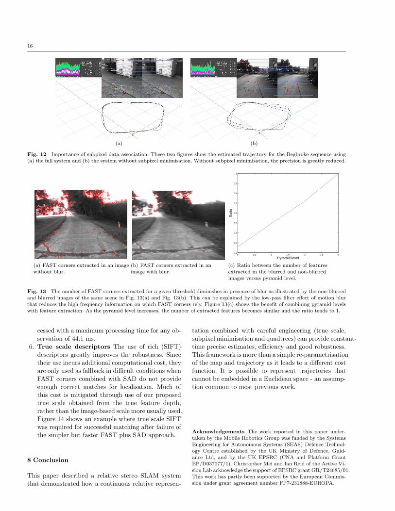
2. Sub-pixel refinement Sub-pixel refinement was

found to be essential to obtain precise trajectory

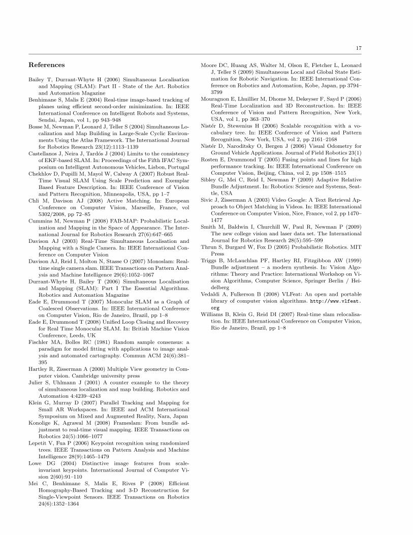
estimates as shown in Fig. 12.3. Multi-level quadtrees Robustness to motion blur

can be improved by using quadtrees over 2-4 image

pyramid levels. Figure 13 illustrates the effect ofpyramid levels on feature extraction.

4. Changes in illumination A simple mechanism to

compensate for changes in illumination and low con-trast proved important in outdoor sequences (Fig.

10).

5. Loop closures Figures 7(a)-7(f) show the results

with and without loop closure. Loop closure sub-stantially reduces drift without requiring a global

minimisation. While the loop closure mechanism is

not strictly constant time, 103K keyframes were pro-

16

(a) (b)

Fig. 12 Importance of subpixel data association. These two figures show the estimated trajectory for the Begbroke sequence using(a) the full system and (b) the system without subpixel minimisation. Without subpixel minimisation, the precision is greatly reduced.

(a) FAST corners extracted in an imagewithout blur.

(b) FAST corners extracted in animage with blur.

0 0.5 1 1.5 2 2.5 30.2

0.3

0.4

0.5

0.6

0.7

0.8

0.9

1

Pyramid level

Rat

io

(c) Ratio between the number of featuresextracted in the blurred and non-blurredimages versus pyramid level.

Fig. 13 The number of FAST corners extracted for a given threshold diminishes in presence of blur as illustrated by the non-blurredand blurred images of the same scene in Fig. 13(a) and Fig. 13(b). This can be explained by the low-pass filter effect of motion blurthat reduces the high frequency information on which FAST corners rely. Figure 13(c) shows the benefit of combining pyramid levels

with feature extraction. As the pyramid level increases, the number of extracted features becomes similar and the ratio tends to 1.

cessed with a maximum processing time for any ob-

servation of 44.1 ms.

6. True scale descriptors The use of rich (SIFT)descriptors greatly improves the robustness. Since

their use incurs additional computational cost, they

are only used as fallback in difficult conditions when

FAST corners combined with SAD do not provideenough correct matches for localisation. Much of

this cost is mitigated through use of our proposed

true scale obtained from the true feature depth,rather than the image-based scale more usually used.

Figure 14 shows an example where true scale SIFT

was required for successful matching after failure ofthe simpler but faster FAST plus SAD approach.

8 Conclusion

This paper described a relative stereo SLAM system

that demonstrated how a continuous relative represen-

tation combined with careful engineering (true scale,

subpixel minimisation and quadtrees) can provide constant-

time precise estimates, efficiency and good robustness.This framework is more than a simple re-parametrisation

of the map and trajectory as it leads to a different cost

function. It is possible to represent trajectories that

cannot be embedded in a Euclidean space - an assump-tion common to most previous work.

Acknowledgements The work reported in this paper under-

taken by the Mobile Robotics Group was funded by the SystemsEngineering for Autonomous Systems (SEAS) Defence Technol-ogy Centre established by the UK Ministry of Defence, Guid-ance Ltd, and by the UK EPSRC (CNA and Platform GrantEP/D037077/1). Christopher Mei and Ian Reid of the Active Vi-sion Lab acknowledge the support of EPSRC grant GR/T24685/01.This work has partly been supported by the European Commis-sion under grant agreement number FP7-231888-EUROPA.

17

References

Bailey T, Durrant-Whyte H (2006) Simultaneous Localisationand Mapping (SLAM): Part II - State of the Art. Roboticsand Automation Magazine

Benhimane S, Malis E (2004) Real-time image-based tracking ofplanes using efficient second-order minimization. In: IEEEInternational Conference on Intelligent Robots and Systems,Sendai, Japan, vol 1, pp 943–948

Bosse M, Newman P, Leonard J, Teller S (2004) Simultaneous Lo-calization and Map Building in Large-Scale Cyclic Environ-ments Using the Atlas Framework. The International Journalfor Robotics Research 23(12):1113–1139

Castellanos J, Neira J, Tardos J (2004) Limits to the consistencyof EKF-based SLAM. In: Proceedings of the Fifth IFAC Sym-posium on Intelligent Autonomous Vehicles, Lisbon, Portugal

Chekhlov D, Pupilli M, Mayol W, Calway A (2007) Robust Real-Time Visual SLAM Using Scale Prediction and ExemplarBased Feature Description. In: IEEE Conference of Visionand Pattern Recognition, Minneapolis, USA, pp 1–7

Chli M, Davison AJ (2008) Active Matching. In: EuropeanConference on Computer Vision, Marseille, France, vol5302/2008, pp 72–85

Cummins M, Newman P (2008) FAB-MAP: Probabilistic Local-ization and Mapping in the Space of Appearance. The Inter-national Journal for Robotics Research 27(6):647–665

Davison AJ (2003) Real-Time Simultaneous Localisation and

Mapping with a Single Camera. In: IEEE International Con-ference on Computer Vision

Davison AJ, Reid I, Molton N, Stasse O (2007) Monoslam: Real-

time single camera slam. IEEE Transactions on Pattern Anal-ysis and Machine Intelligence 29(6):1052–1067

Durrant-Whyte H, Bailey T (2006) Simultaneous Localisationand Mapping (SLAM): Part I The Essential Algorithms.Robotics and Automation Magazine

Eade E, Drummond T (2007) Monocular SLAM as a Graph ofCoalesced Observations. In: IEEE International Conference

on Computer Vision, Rio de Janeiro, Brazil, pp 1–8Eade E, Drummond T (2008) Unified Loop Closing and Recovery

for Real Time Monocular SLAM. In: British Machine VisionConference, Leeds, UK

Fischler MA, Bolles RC (1981) Random sample consensus: aparadigm for model fitting with applications to image anal-ysis and automated cartography. Commun ACM 24(6):381–395

Hartley R, Zisserman A (2000) Multiple View geometry in Com-puter vision. Cambridge university press

Julier S, Uhlmann J (2001) A counter example to the theory

of simultaneous localization and map building. Robotics andAutomation 4:4239–4243

Klein G, Murray D (2007) Parallel Tracking and Mapping forSmall AR Workspaces. In: IEEE and ACM InternationalSymposium on Mixed and Augmented Reality, Nara, Japan

Konolige K, Agrawal M (2008) Frameslam: From bundle ad-justment to real-time visual mapping. IEEE Transactions onRobotics 24(5):1066–1077

Lepetit V, Fua P (2006) Keypoint recognition using randomizedtrees. IEEE Transactions on Pattern Analysis and MachineIntelligence 28(9):1465–1479

Lowe DG (2004) Distinctive image features from scale-invariant keypoints. International Journal of Computer Vi-sion 2(60):91–110

Mei C, Benhimane S, Malis E, Rives P (2008) Efficient

Homography-Based Tracking and 3-D Reconstruction forSingle-Viewpoint Sensors. IEEE Transactions on Robotics24(6):1352–1364

Moore DC, Huang AS, Walter M, Olson E, Fletcher L, LeonardJ, Teller S (2009) Simultaneous Local and Global State Esti-mation for Robotic Navigation. In: IEEE International Con-ference on Robotics and Automation, Kobe, Japan, pp 3794–3799

Mouragnon E, Lhuillier M, Dhome M, Dekeyser F, Sayd P (2006)

Real-Time Localization and 3D Reconstruction. In: IEEEConference of Vision and Pattern Recognition, New York,USA, vol 1, pp 363–370

Nister D, Stewenius H (2006) Scalable recognition with a vo-

cabulary tree. In: IEEE Conference of Vision and PatternRecognition, New York, USA, vol 2, pp 2161–2168

Nister D, Naroditsky O, Bergen J (2006) Visual Odometry forGround Vehicle Applications. Journal of Field Robotics 23(1)

Rosten E, Drummond T (2005) Fusing points and lines for highperformance tracking. In: IEEE International Conference onComputer Vision, Beijing, China, vol 2, pp 1508–1515

Sibley G, Mei C, Reid I, Newman P (2009) Adaptive RelativeBundle Adjustment. In: Robotics: Science and Systems, Seat-tle, USA

Sivic J, Zisserman A (2003) Video Google: A Text Retrieval Ap-

proach to Object Matching in Videos. In: IEEE InternationalConference on Computer Vision, Nice, France, vol 2, pp 1470–1477

Smith M, Baldwin I, Churchill W, Paul R, Newman P (2009)

The new college vision and laser data set. The InternationalJournal for Robotics Research 28(5):595–599

Thrun S, Burgard W, Fox D (2005) Probabilistic Robotics. MIT

PressTriggs B, McLauchlan PF, Hartley RI, Fitzgibbon AW (1999)

Bundle adjustment – a modern synthesis. In: Vision Algo-rithms: Theory and Practice: International Workshop on Vi-sion Algorithms, Computer Science, Springer Berlin / Hei-delberg

Vedaldi A, Fulkerson B (2008) VLFeat: An open and portablelibrary of computer vision algorithms. http://www.vlfeat.

org

Williams B, Klein G, Reid DI (2007) Real-time slam relocalisa-tion. In: IEEE International Conference on Computer Vision,

Rio de Janeiro, Brazil, pp 1–8