rr643 assessing and modelling the uncertainty in fatigue crack

Executive Health and Safety

Assessing and modelling the uncertainty in fatigue crack growth in structural steels

Prepared by the University of Aberdeen and Genesis Oil and Gas Consultants Limited for the Health and Safety Executive 2008

RR643 Research Report



Michael Baker University of Aberdeen King’s College Aberdeen AB24 3FX

Ian Stanley Genesis Oil and Gas Consultants Ltd 262 High Holborn London WC1V 7NA

The prediction of the fatigue life of steel structures can be carried out in a number of different ways. A common method at the design stage is to use the so-called S-N approach using design data from a standard such as BS 7910. However, for existing structures containing defects of a known or postulated size, a fatigue life assessment is generally carried out using fracture mechanics. In keeping with normal engineering practice, it is usual to calculate conservative (safe) estimates of fatigue life, although occasionally best estimates may also be of interest. For more advanced structural assessments, reliability-based methods can be used to calculate the remaining life corresponding to a number of different probabilities of failure (eg 10-4, 10-6). The motivation for the research reported here was the need to improve the current methods of reliability assessment for structures, and in particular steel offshore structures approaching the end of their design lives. As part of this research, work was carried out to investigate the variability in the fatigue crack growth of steels and the way in which the corresponding uncertainties could best be incorporated into the assessment process. This included the fatigue testing of specimens of BS 4360: 1990 Grade 50DD steel with the explicit aim of studying the variability in crack growth under different conditions. The results of these tests are presented in this research report. The relatively large uncertainties associated with fatigue crack growth behaviour, even within relatively homogenous sets of specimens, means that the variance in the predicted fatigue life is relatively large. It has been shown, however, that the use of fatigue crack growth rate data from relatively early in the life of a particular structure can significantly reduce this uncertainty and improve the reliability predictions through the process of reliability updating.

This report and the work it describes were funded by the Health and Safety Executive (HSE). Its contents, including any opinions and/or conclusions expressed, are those of the authors alone and do not necessarily reflect HSE policy.

HSE Books

© Crown copyright 2008

First published 2008

All rights reserved. No part of this publication may be reproduced, stored in a retrieval system, or transmitted in any form or by any means (electronic, mechanical, photocopying, recording or otherwise) without the prior written permission of the copyright owner.

Applications for reproduction should be made in writing to:Licensing Division, Her Majesty’s Stationery Office,St Clements House, 2-16 Colegate, Norwich NR3 1BQor by e-mail to [email protected]

ACKNOWLEDGEMENTS

The work described in this report was part of a research project Improved generic strategies and methods for reliability-based structural integrity assessment supported by the Engineering and Physical Sciences Research Council and the Health and Safety Executive.

ii

CONTENTS

1 INTRODUCTION 11.1 Background 11.2 Traditional Approach to Fatigue Crack Growth Prediction 11.3 Comparison with Other Fatigue Crack Growth Experiments 51.4 Introduction to the Current Research 6

2 DETAILS OF EXPERIMENTAL PROGRAMME 92.1 Test Specimens 9

2.1.1 Compact tension specimens 112.1.2 Beam specimens 132.1.3 Stress-strain properties 14

2.2 Fatigue Loading and Pre-Cracking 142.3 Crack Growth Measurement 14

3 ANALYSIS OF FATIGUE CRACK GROWTH RATES 173.1 Introduction 173.2 Raw Data Reduction 17

3.2.1 Localised within-specimen variations in crack growth rate 173.2.2 Data reduction 21

3.3 Analysis of Non-welded Beam Specimens 233.3.1 Introduction 233.3.2 Non-welded beam specimens 23

3.4 Analysis of Welded Beam Specimens 253.5 Analysis of Non-welded Compact Tension Specimens 263.6 Analysis of Welded Compact Tension Specimens 30

4 INTERPRETATION OF EXPERIMENTAL FINDINGS 334.1 Introduction 334.2 Within and Between Specimen Variability in Fatigue Crack Growth Rates 33

4.2.1 Short-term variability in fatigue crack growth in the parent plate 334.2.2 Short-term variability in fatigue crack growth in the weld material 344.2.3 Long-term variability in fatigue crack growth in the parent plate 354.2.4 Long-term variability in fatigue crack growth in the weld material 36

5 DEVELOPMENT OF STOCHASTIC FATIGUE CRACK GROWTH MODELS 395.1 Introduction 395.2 Model Based on the Virkler Data Set 40

5.2.1 Introduction 405.2.2 Stochastic model for Virkler data 415.2.3 a priori model based on Virkler data 425.2.4 Graphical representation of model 445.2.5 Reliability updating 45

5.3 Models for Structural Steels Based on Current Experimental Data 475.3.1 Simple linear a priori crack growth model 495.3.2 More advanced crack growth models 525.3.2.1 Generic Model Description 525.3.2.2 Special property of crack growth curves 525.3.2.3 Generic non-linear model 545.3.3 Application of generic non-linear model 55

iii

6 DISCUSSION AND CONCLUSIONS 57

REFERENCES AND BIBLIOGRAPHY 59

APPENDIX I: Experimental fatigue data – non-welded beams 63APPENDIX 2: Experimental fatigue data – welded beams 67APPENDIX 3: Experimental fatigue data – non-welded CT specimens 69APPENDIX 4: Experimental fatigue data – welded CT specimens 83

iv

EXECUTIVE SUMMARY

The prediction of the fatigue life of steel structures can be carried out in a number of different ways. A common method at the design stage is to use the so-called S-N approach using design data from a standard such as BS 7910. However, for existing structures containing defects of a known or postulated size, a fatigue life assessment is generally carried out using fracture mechanics. For such an analysis it is necessary to use an appropriate crack growth model (e.g. the simple Paris law, or a two-stage crack growth relationship) and to know values of the relevant parameters for the type of steel in question and loading environment (e.g. marine). In keeping with normal engineering practice, it is usual to calculate conservative (safe) estimates of fatigue life, although occasionally best estimates may also be of interest.

For more advanced structural assessments, reliability-based methods can be used to calculate the remaining life corresponding to a number of different probabilities of failure (e.g. 10-4, 10-6); or conversely to estimate the probability of failure for one or more specified time periods (e.g. 1, 10 and 20 years of continued service life).

The information and data required for routine engineering assessments and for reliability-based approaches are essentially the same, but the information is used in different ways. For the former, the industry approach has been to develop S-N curves and da dN versus / ΔK relationships from test data which are sufficiently conservative (e.g. mean minus two standard deviation curves). For reliability-based assessments on the other hand, information is required on the probability distributions of the parameters that are used in the engineering calculations to predict fatigue crack growth, as well as a quantitative evaluation of the uncertainties associated with the fatigue crack growth model itself, known as model uncertainty.

The motivation for the research reported here was the need to improve the current methods of reliability assessment for structures, and in particular steel offshore structures approaching the end of their design lives, in order to justify their continued use or not, as the case may be. The research project entitled ‘Improved generic strategies and methods for reliability-based structural integrity assessment’ sponsored by EPSRC and HSE was aimed at finding the best way in which information gained during in-service inspection and monitoring can be used to improve the prediction of the remaining useful life on a probabilistic basis. As part of this research, work was carried out to investigate the variability in the fatigue crack growth of steels and the way in which the corresponding uncertainties could best be incorporated into the assessment process. This included the fatigue testing of specimens of BS 4360: 1990 Grade 50DD steel with the explicit aim of studying the variability in crack growth under different conditions. The results of these tests are presented in this research report.

Fatigue tests were carried on compact tension and single edge notched beam specimens cut from a single slab of 50 mm thick Grade 50DD steel, 840 mm long × 755 mm wide, which had first been cut and then welded with a double V butt weld. Seven beam and 28 compact tension (CT) specimens were prepared and tested, some involving the propagation of the fatigue crack through the weld and the remainder with the crack in the parent plate. With one exception, the beams were 50 mm × 50mm in cross-section, but the CT specimens were prepared in a range of sizes and orientations, so that the crack growth rate and its variability could be studied for cracks propagating in the through-thickness direction, across the plate, up through the weld and lastly along the weld in the direction of welding. The CT specimens were also prepared in a number of different thicknesses ranging from 5 mm to 50 mm in order to investigate the influence of the length of the crack front, if any, on the variability in growth rate.

Up to the present time, fracture mechanics-based fatigue assessment has been based on

v

conservative design curves, which in turn are based on pooled experimental crack growth data obtained at different values of range of stress intensity, ΔK, and from a number of sources – as, for example, in the development of British Standard BS7910: 2005. The approach has been to

/set the design log (da dN ) versus log (ΔK ) relationship at two standard deviations above mean

regression line based on available experimental data. However, the sources of the considerable variability in the crack growth data published in the literature are not really known. In the present experimental work it was therefore not known in advance what degree of variability in crack growth rates would be present and what differences would be found.

The aims of the physical tests were therefore to study, and where possible characterise, the mean fatigue crack growth behaviour and the variability about that mean: • within each specimen as the crack grew • between different but nominally similar specimens, and • between different specimens, with respect to:

i. specimen thickness ii. direction of crack propagation within the plate

iii. the material being sampled by the crack front (parent plate or weld metal) iv. the geometry of the specimen being tested (beam and CT specimens)

The test programme has revealed new insights into each of the above sources of variability. Basically, the variability in fatigue crack growth rate can be decomposed into local fluctuations about the mean rate at each value of range of stress intensity ΔK, and variations in the mean rate with change in ΔK.

Study of the local fluctuations show that the coefficient of variation (COV) of the crack growth rate da/dN can be expressed in the form:

da βCOV =α (ΔK )

dN

which is of the same basic form as the Paris law. The magnitude of these local fluctuations in growth rate are also dependent on the increment of crack extension over which the growth rate is calculated and can be shown to become negligible for crack increments of about 0.5 mm or more. These fluctuations are of no practical significance, except in relation to the measurement of crack growth during the inspection and monitoring of structures.

The more important question of the variability in the overall crack growth relationship, /log (da dN ) versus log (ΔK ) , and the differences that can arise, has also been addressed in the

current work. For all the beam specimens it was found that the basic crack growth curve tended to be curvilinear rather than linear, and that the crack growth rate was somewhat higher in the across-plate direction as compared with the through-thickness direction. For the welded beams, relatively large differences were found between specimens in which the crack propagated up through the weld as opposed to along the weld, with the former being a factor of up to six times faster.

For the non-welded compact tension specimens, it was found that there were significant variations in the overall crack growth rate between specimens of different thickness, with the thinner specimens fatiguing more slowly than the thicker ones at the same value of ΔK. The specimens that were cut vertically through the plate behaved in a similar way to the larger specimens that were cut with faces parallel to the face of the plate, but had somewhat less variability.

vi

Comparison of the non-welded CT specimen results with present design curves shows that for the higher values of ΔK some of the specimens had growth rates in excess of that predicted by the design curves, with the implication that the design curves may not be sufficiently conservative.

Much larger variations in crack growth rate were found for the welded CT specimens, with mean crack growth rates differing by up to an order of magnitude. These specimens also showed a marked size effect, with the thicker specimens having a significantly higher growth rate than the thinner ones. Many of the welded specimens, however, exhibited significantly lower growth rates than similar specimens taken from the parent plate. Of particular note was the slow growth rate in the specimens in which the fatigue crack was propagating across the plate along the weld, with the crack front sampling the full weld thickness.

The main objective of this research has been to improve models for use in the reliability assessment of welded structures failing by fatigue. These specific issues are discussed in Section 5 in which models based on both the 1978 data set obtained by Virkler for thin aluminium specimens and the data obtained in the present experimental work for structural steels are used to develop new approaches to modelling. The strong correlation between the quantities m and log C of the Paris Law relationship has been studied using these data sets, and leads to an a priori model involving only m and two independent error terms ε1 and ε2. However, the relatively large uncertainties associated with fatigue crack growth behaviour, even within relatively homogenous sets of specimens, means that the variance in the predicted fatigue life is relatively large. It has been shown, however, that the use of fatigue crack growth rate data from relatively early in the life of a particular structure can significantly reduce this uncertainty and improve the reliability predictions through the process of reliability updating.

vii

1 INTRODUCTION

1.1 BACKGROUND

The prediction of the fatigue life of steel structures can be carried out in a number of different ways. A common method at the design stage is to use the so-called S-N approach using design data from a standard such as BS 7910: 2005. However, for existing structures containing defects of a known or postulated size, a fatigue life assessment is generally carried out using fracture mechanics. For such an analysis it is necessary to use an appropriate crack growth model (e.g. the simple Paris law, or a two-stage crack growth relationship) and to know values of the relevant parameters for the type of steel in question and loading environment (e.g. marine). In keeping with normal engineering practice, it is usual to calculate conservative (safe) estimates of fatigue life, although occasionally best estimates may also be of interest.

For more advanced structural assessments, reliability-based methods (e.g. Thoft-Christensen and Baker 1982, Madsen et al 1986, Melchers 1999) can be used to determine the remaining life corresponding to one or more probabilities of failure (e.g. 10-4, 10-6); or conversely to estimate the probability of failure for one or more specified time periods (e.g. 1, 10 and 20 years of continued service life).

The information and data required for routine engineering assessments and for reliability-based approaches are essentially the same, but the information is used in different ways. For the former, the industry approach has been to develop S-N curves and da dN versus / ΔK relationships from test data which are sufficiently conservative (e.g. mean minus two standard deviation curves). For reliability-based assessments on the other hand, information is required on the probability distributions of the parameters that are used in the engineering calculations to predict fatigue crack growth, as well as a quantitative evaluation of the uncertainties associated with the fatigue crack growth model itself, known as model uncertainty.

The motivation for the research reported here was the need to improve the current methods of reliability assessment for structures, and in particular steel offshore structures approaching the end of their design lives, in order to justify their continued use or not, as the case may be. The research project entitled ‘Improved generic strategies and methods for reliability-based structural integrity assessment’ sponsored by the Engineering and Physical Sciences Research Council (EPSRC) and the Health and Safety Executive (HSE) was aimed at finding the best way in which information gained during in-service inspection and monitoring can be used to improve the prediction of the remaining useful life on a probabilistic basis. As part of this research, work was carried out to investigate the scatter or variability in the fatigue crack growth of steels and the way in which this could best be taken into account in the assessment process. This included the fatigue testing of specimens of BS 4360: 1990 Grade 50DD steel (now BS EN 10025: Part 2: 2004, Grade S355K2) with the explicit aim of studying the variability in crack growth under different conditions. The results of these tests are presented in Section 3 of this research report and a review of the findings is given in Section 4. In Section 5, models for use in reliability analysis and reliability updating are introduced and reviewed, together with some sample calculations based on the findings of the experimental part of the programme.

1.2 TRADITIONAL APPROACH TO FATIGUE CRACK GROWTH PREDICTION

To predict the fatigue life of steel structures containing small defects (e.g. weld defects) using a fracture mechanics approach it is necessary to know or postulate the relationship between the range of stress intensity ΔK and the rate of crack propagation da dN (the increment of crack / growth per stress cycle), where a is the defect size and N is the number of cycles of applied

1

load. Various theoretical models are available, the best known and simplest being that due to Paris and Erdogan (1963), namely:

da = C (ΔK )m (1) dN

where for deterministic assessments C and m are generally taken to be constants.

In the early days of fracture mechanics, the usual approach to developing a suitable basis for design or assessment was to take experimental fatigue crack growth data for the relevant material, and to plot an upper bound curve which was then taken as the governing deterministic relationship (e.g. Maddox 1974, Fig 18, p60), as illustrated in Figure 1. The use of an upper bound is likely to be conservative (safe) but its equation and the corresponding values of C and m obviously depend on the size of the data set, and whether the population is homogeneous. However, of equal importance in assessing the integrity of a structural component failing by fatigue is the uncertainty in the calculated values of range of stress intensity, ΔK , and how this is treated in the design or assessment process. This latter issue will not be considered in the present report.

Figure 1 Fatigue crack growth data for structural carbon-manganese steels, tested at stress ratio R = 0, from Maddox (1974)

2

More recently, formal statistical methods have been used to obtain ‘safe’ design curves for fatigue for different types of steel under various environmental conditions. For example, King, Stacey and Sharp (1996) and King (1998) in a review of fatigue crack growth rates of steels in

/air and seawater have developed two-stage linear log (da dN ) versus log (ΔK ) relationships for

/a range of steels and environmental conditions based on linear regression of log (da dN ) on

log (ΔK ) . By estimating the standard deviation of the data points about each regression line, it

is then possible to construct ‘design lines’ that correspond to the mean line plus two standard deviations. Pooled data from a number of different sources for ferritic steels tested in air at a stress ratio R of 0.1 are shown in Figure 2 (King 1998).

Figure 2 Fatigue crack growth rates for ferritic steels tested in air, at stress ratio R = 0.1, from King (1998) – pooled data

King has determined the mean and design lines for the two stages to be:

Stage 1: Mean line 26 8.16 / 1.21 10 da dN K−= × Δ Design line 26 8.16 / 4.37 10 da dN K−= × Δ

Stage 2: Mean line 13 2.88 / 3.98 10 da dN K−= × Δ Design line 13 2.88 / 6.77 10 da dN K−= × Δ

and these are shown in Figure 3 over a practical range of ΔK , together with lines drawn at mean minus two standard deviations to illustrate the range within which most observed crack growth rates are likely to occur.

3

This approach has been adopted in the development of BS7910 and provides design curves which are obviously conservative in comparison with the mean curves. However, the data used to produce these relationships have been pooled from a series of different tests in which the fatigue crack growth rate has been determined at different values of ΔK . What is not possible to determine from these data is whether a crack that is growing at a relatively low rate compared with the mean rate (at a particular value of ΔK ) will continue to grow at that rate, or whether the rate will increase, or even decrease. Similarly, will a crack that is found to be growing at a high rate, corresponding say to the design curve value (at a known value of ΔK ), continue at that rate and what are the chances that the rate will increase even further?

ΔK -3/2)

//

l

1.E-08

1.E-07

1.E-06

1.E-05

1.E-04

1.E-03

1.E-02

100 1000 10,000

(Nmm

da

dN (

mm

cyc

e)

Figure 3 Mean and design curves for fatigue of ferritic steels at stress ratio R = 0.1, based on crack growth models proposed by King (1998) and ignoring threshold effects

The questions raised above have a bearing on:

• the degree of conservatism implied by the fatigue design curves in, for example, BS7910, and

• how fatigue crack growth rates measured in actual structures during or between successive inspections are used to predict remaining service life before failure occurs.

In the above, the simplifying assumption is made that the structural component is subjected to known constant amplitude loading and that the fatigue crack is of a known size and shape, thus enabling the stress intensity K to be determined. It is also assumed that, under normal conditions, K and thus the range of stress intensity ΔK will increase with crack growth. However, for non-constant amplitude loading and for complex structures where some load redistribution may take place as a result of the change in stiffness arising from the presence of the crack, the behaviour will be more complex. These issues are not considered here.

The basic question, therefore, is whether the variability in fatigue crack growth rate shown by the data in Figure 2 is mainly a result of variations in fatigue properties of the steels from one test sample to another, as the form of analysis undertaken by King (1998) implies, or whether there is a significant component of within-sample variability which is contributing to the observed overall variability in growth rate. In the case of fatigue cracks growing in weld material, within-weld variability seems highly likely as the crack tip samples the different weld beads, but the within-plate variability of the parent steel is less well studied. The work described in this report aims to explore these questions.

4

1.3 COMPARISON WITH OTHER FATIGUE CRACK GROWTH EXPERIMENTS

One set of data which has received considerable attention is that obtained by Virkler et al (1978, 1979) on a set of 68 nominally identical centre-cracked aluminium alloy panels 152 mm wide and 2.54 mm thick, subjected to constant amplitude loading at a stress ratio R = 0.2. The number of loading cycles for the tip of the crack to advance a predetermined increment Δa = 0.2 mm was recorded from an initial crack length of 9.0 mm to a final length of 49.8 mm (0.4 mm and 0.8 mm increments were also used in the later stages of growth). These data are plotted in Figure 4 which shows the wide variation in the number of cycles required to grow the cracks.

l

Cra

ck le

ng th

(m

m)

Number of cyc es

50

40

30

20

10

0

0 50,000 100,000 150,000 200,000 250,000 300,000 350,000

Figure 4 Variation in crack length with number of cycles of applied stress for 68 nominally identical specimens [plotted from Virkler et al (1978) data set]

To illustrate the fact that the fatigue crack growth rate does indeed vary for individual specimens as the crack extends, data for a small number of the Virkler specimens have been

/selected and are shown in Figure 5 in terms of da dN versus ΔK . To filter out the extreme fluctuations in da dN which are present in the raw experimental data, the crack growth rates / shown here are moving averages over ten 0.2 mm increments of crack growth (i.e. 2 mm). The stress intensity factors have been computed from Rooke and Cartwright (1976). Figure 5 clearly demonstrates that for individual specimens there are marked fluctuations in crack growth rate as well as significant differences between specimens at particular values of ΔK .

In the present work, a similar study to that reported by Virkler et al has been carried out in relation to the fatigue behaviour of Grade 50 DD steel used in the construction of fixed offshore jacket structures, as described in the following sections.

5

//

l

ΔK /2)

1.0E-05

1.0E-04

1.0E-03

100 500 1,000

dadN

(m

mcy

ce)

(Nmm -3

Figure 5 Variation in crack growth rate with stress intensity factor for seven nominally identical specimens tested at constant stress range

[Virkler et al (1978) data set]

1.4 INTRODUCTION TO THE CURRENT RESEARCH

As previously discussed, the main motivation for the research reported here was the need to improve the current methods for the reliability assessment of structures, particularly those susceptible to failure by fatigue. To date the main approach to fatigue reliability assessment using fracture mechanics has been to assign probability distributions to the parameters C and m in the Paris Law, or to the parameters C, C’, m and m’ in the case of an assumed two-stage fatigue crack growth relationship, and then to use a first-order or second-order reliability method (FORM/SORM) to compute the probability that failure will occur within a specified period of time (e.g. Madsen et al 1986, Righiniotis and Chryssanthopoulos 2003). However, such an approach implies that, for any given structure, the parameters C and m are fixed in magnitude but with values that are not precisely known. A study of Figure 5 shows that the situation is more complex than this and that, in addition to uncertainties in C and m (or log C and log m), there are considerable approximations in assuming a linear or bi-linear relationship

/between log (da dN ) and log (ΔK ) when considering the growth of any particular fatigue

crack. The implications of this are discussed further in a later section.

The primary objectives of the research described in this report were to undertake a series of carefully controlled measurements of the fatigue crack growth rate of a weldable structural steel typical of that used in the construction of fixed steel offshore installations, in order to study the variability in growth rate with crack extension under different conditions; and thus to build suitable stochastic models for crack growth which would be consistent with advanced methods of structural reliability analysis.

Tests were planned in order to answer a number of specific questions: • How does the rate of crack growth vary over short periods of time and over relatively small

amounts of crack extension?

6

• What are the errors in assuming that fatigue cracking can be modelled by a linear or bilinear law when considering a single crack growing under constant amplitude loading; and what is the corresponding model uncertainty?

• How does the crack growth rate vary between nominally identical specimens when loaded under nominally identical conditions?

• How does the thickness of the specimen and hence the length of the crack front influence the above?

• Is the rate of crack growth influenced by the direction of propagation in a plate? • How are all the above influenced when the crack grows through regions of welded material

where the crack front is likely to be sampling a range of micro-structures and where high magnitudes of residual stresses will be present?

The following sections of this report deal with details of the physical tests conducted, an analysis of the fatigue data obtained, and the implications for the modelling of fatigue both in deterministic and reliability-based assessments. The final section deals with fatigue modelling, reliability analysis and reliability updating.

7

2 DETAILS OF EXPERIMENTAL PROGRAMME

2.1 TEST SPECIMENS

The decision was made to undertake a series of fatigue tests on 50DD structural grade steel to explore the variability in fatigue crack growth rates both within specimens and between specimens. Consideration was also given to the need to assess any differences in this variability between welded and non-welded material. This section outlines the methodology adopted for the fatigue tests undertaken.

After undertaking some prototype tests on a series of single edge notched beam specimens, the main series of tests was conducted on beam (denoted B) and compact tension (denoted CT) specimens cut from a single 50 mm thick plate produced to BS 4360: 1990 Grade 50DD (now designated EN 10025: part 2: 2004 Grade S355K2). The plate measured 840 mm × 755 mm and allowed the production of 35 specimens as shown in Figure 6, with the specimens comprising either as-rolled parent plate or part weldment. Prior to preparation of the individual specimens, the whole plate was cut into two pieces and then welded in order to produce a typical plate butt weld from which fatigue specimens could be cut, in order to allow comparison between welded and non-welded material. The plate was profile cut and then welded with a double V-butt weld in accordance with ASME 1X and API 6A/16A procedures.

The total of 35 test pieces was made up of 7 single edge notched beam and 28 CT specimens. As shown in Figure 6, the specimens were cut in such a way as to be able to study the differences in the fatigue crack growth rate:

• between different positions within each specimen (local spatial variability) • between specimens of different thickness • between cracks growing in the through-thickness direction and those growing in the

direction of rolling or across the plate • between cracks growing in the as-rolled parent plate and the weld zone, and • between beam and CT specimens

For ease of handling, the welded plate was initially cut into five sub-plates A, B, C, D and E, as shown in Figure 6, using a profile gas cutter. The heat affected edges were then mechanically removed using a band saw prior to specimen manufacture to ensure that the specimens would not being influenced by the thermal cutting process. However the plate was not subjected to post-weld heat treatment with the result that the test pieces containing weld material would have been influenced by reasonably high levels of welding-induced residual stress. This was intentional and was considered to be representative of typical welded construction.

In Figure 6, the beam test pieces are marked as A1a, A1b, A2, B1, B2, E1 and E2. Beams A1a and A1b were nominally identical and of square cross-section, and were tested in three-point bending so that the fatigue crack grew upwards through the thickness of the plate, but within the weld metal. Beam A2 was similar in dimensions, but with the fatigue crack propagating across the plate, but also within the weld metal. Beams B1 and B2 were from adjacent pieces of parent plate, but with the fatigue crack growing across the plate and upwards through the plate respectively. Beam E2 was nominally identical to B2 but from a different region of the plate, and finally beam E1 was similar to beam B1, but of double the depth (i.e. 100 mm × 50 mm in cross-section).

Figure 6 also shows the positions, sizes and orientations of the 28 CT specimens. Those denoted C1 to C10 were with the fatigue crack in the weldment, whereas D1 to D3 and E1 to E3 were

9

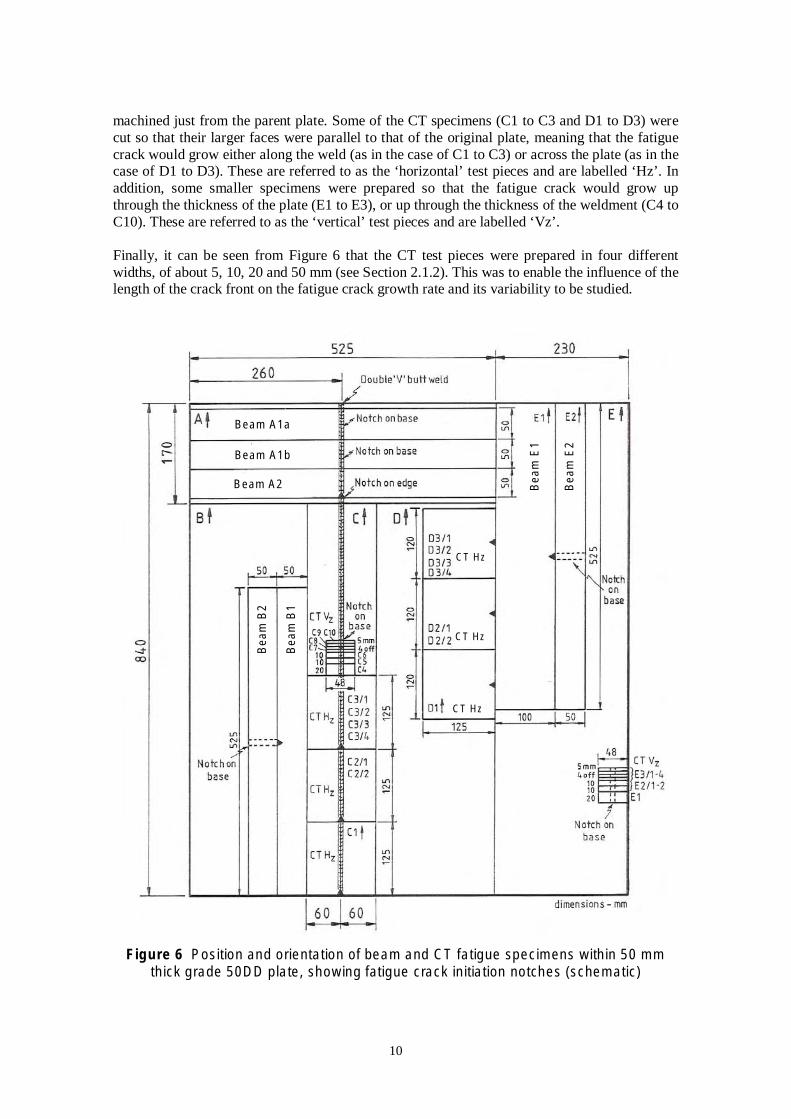
machined just from the parent plate. Some of the CT specimens (C1 to C3 and D1 to D3) were cut so that their larger faces were parallel to that of the original plate, meaning that the fatigue crack would grow either along the weld (as in the case of C1 to C3) or across the plate (as in the case of D1 to D3). These are referred to as the ‘horizontal’ test pieces and are labelled ‘Hz’. In addition, some smaller specimens were prepared so that the fatigue crack would grow up through the thickness of the plate (E1 to E3), or up through the thickness of the weldment (C4 to C10). These are referred to as the ‘vertical’ test pieces and are labelled ‘Vz’.

Finally, it can be seen from Figure 6 that the CT test pieces were prepared in four different widths, of about 5, 10, 20 and 50 mm (see Section 2.1.2). This was to enable the influence of the length of the crack front on the fatigue crack growth rate and its variability to be studied.

CT Hz

CT Hz

CT Hz

Beam A1a

Beam A1b

Beam A2

Bea

m B

2

Bea

m B

1

Bea

m E

1

Bea

m E

2

Figure 6 Position and orientation of beam and CT fatigue specimens within 50 mm thick grade 50DD plate, showing fatigue crack initiation notches (schematic)

10

a

W =

39

mm

a

W =

39

mm

2.1.1 Compact tension specimens

Where possible the dimensions of the CT specimens were sized in accordance with the ratios given in BS 6835-1 (1998), thus allowing standard solutions for the stress intensities K to be used (Murakami 1987). For non-standard geometries, stress intensity factors were calculated directly by finite element analysis using ABAQUS (2002) and the crack-block model available through ZENCRACK (2004). The detailed results have been reported by Nahar Hamid (2006).

For the CT specimens cut vertically through the plate thickness (labelled as Vz CT), the specimen widths B were nominally 5, 10 and 20 mm. For the CT specimens cut within the plate thickness (labelled as Hz CT ), the widths were nominally 8.1 mm, 21.9 mm and 50 mm. These dimensions were governed by cutting and machining requirements where more than one specimen was being cut within the thickness of the plate. Further details of the CT specimens are shown in Figures 7 to 10.

1 1 32 2 4_ _ __ _ _1 2 3 32 3 3E E E EE E E 0.6 W 0.6 W T T T TT T TC C C CC C C

zV zV zV zVzV zV zV

t = 5

0 m

m

1.25

W

20 10 10 5 5 5 5

Figure 7 Details of 7 ‘vertical’ CT specimens Vz CT E1 to Vz CT E3_4, with fatigue crack growing vertically upwards through the thickness of the parent plate

06 7 8 9 154 C C C C CCC

T T T T TTT 0.6 W 0.6 W

C C C C CCC

z z z z zzz V V V V V VV

t = 5

0 m

m

1.2

5 W

20 10 10 5 5 5 5 Weldment

Figure 8 Details of 7 ‘vertical’ CT specimens Vz CT C4 to Vz CT C10, with fatigue crack growing vertically upwards through the weldment

11

i ii

Pl i

2 No. @ 21.9 mm th ck 4 No. @ 8.1 mm th ck 1 No. @ 50 mm th ck

ate th ckness t = 50 mm

Hz CT D1

Hz CT D2_1

Hz CT D2_2

Hz CT D3_1

Hz CT D3_2

Hz CT D3_3

Hz CT D3_4

1.25 W

a

W = 100 mm

0.6

W0.

6 W

W = 100 mm

Figure 9 Details of 7 ‘horizontal’ CT specimens Hz CT D1 to Hz CT D3_4 cut from the parent plate

i

Pl i

2 No. @ 21.9 mm th ck 4 No. @ 8.1 mm thick 1 No. @ 50 mm thick

ate th ckness t = 50 mm

Hz CT C1

Hz CT C2_1

Hz CT C2_2

Hz CT C3_1

Hz CT C3_2

Hz CT C3_3

Hz CT C3_4

1.25 W

a

W = 100 mm

0.6

W0.

6 W

W = 100 mm

Weldment

NOTE: Width of weldment zone is dependent on the position of the specimen

within the plate depth

Figure 10 Details of 7 ‘horizontal’ CT specimens Hz CT C1 to Hz CT C3_4 cut from the weld zone

12

2.1.2 Beam specimens

The beam specimen sizes were non-standard with respect to their span to depth ratios, the normal requirement in BS 6835-1: 1998 being S = 4W, where S is the beam span and W is the beam depth. The beams were prepared and tested as three-point single edge notch specimens and the stress intensity factor solutions for the differing S to W ratios were obtained from Fett (1998).

Table 1 gives the dimensions of the various beam specimens and information on the direction of crack propagation. The latter is shown more clearly in Figure 11 for the welded beams, A1a, A1b and A2.

Table 1 Details of beam test specimens

Serial No. Span Depth Thickness Direction of fatigue crack S (mm) W (mm) B (mm) propagation

A1a 500 50 50 Upwards through weld

A1b 500 50 50 Upwards through weld

A2 500 50 50 Along the weld

B1 500 50 50 Across the plate

B2 500 50 50 Upwards through plate

E1 500 100 50 Across the plate

E2 500 50 50 Upwards through plate

w

a

B

B

w S

S

a

Crack depth

Beams A1a and A1b

Beam A2

Crack depth

Figure 11 Arrangement of three-point bend test specimens A1a, A1b and A2, showing position of fatigue notch in relation to weldment

13

2.1.3 Stress-strain properties

To characterize the stress-strain characteristics of the parent plate three uni-axial tensile test specimens from different locations and orientations within the plate were prepared and tested in accordance with ASTM E8M (2001). A typical stress strain curve is shown in Figure 12. This is included here as a record of the properties of the material used in the fatigue tests, but these data were also used in a J-integral analysis to examine the effect of modelling crack growth rate as a function of Δ J rather than ΔK , as discussed in Section 4.

Figure 12 Uni-axial stress-strain curve for test plate

2.2 FATIGUE LOADING AND PRE-CRACKING

P

For undertaking fatigue tests, BS 6835-1: 1998 calls for the initial pre-cracking of specimens followed by load reduction until the desired test-loading regime has been achieved. However, to avoid possibly overstressing the specimens before testing under constant amplitude load, a load-increasing strategy was adopted for all specimens. This entailed the application of a cyclic load

min to Pmax, with Pmax corresponding to an initially low stress intensity. This loading was maintained for a sufficiently large number of cycles (e.g. 500,000), following which if no growth had been detected, a somewhat higher load range was applied. This process was continued until steady state growth was detected at which point the loading remained unchanged. All tests were conducted at an applied stress ratio of R = 0.2.

All beam specimens were tested in three-point bending (with the load applied directly above the notch) using an ESH Testing Machine. CT specimens were tested on an Instron 8500. All tests were carried out at a loading frequency of 10 Hz. This was largely governed by the need to measure the crack growth at sufficiently frequent intervals, but was also influenced by the compliance of the testing machines.

2.3 CRACK GROWTH MEASUREMENT

Accurate measurement of crack size during the fatigue tests was one of the most important aspects of the experimental work. Following the initial prototype tests, it was decided that it was important to measure the crack growth at a number of positions along the crack front, especially for the thicker test pieces. Another factor that became clear from the prototype tests was that the

14

tests needed to be run continuously wherever possible, because stopping and starting the cyclic loading was observed to lead to transients in the fatigue crack growth rate, even though the loads were kept below Pmax at all times. This meant that the fatigue crack growth measurement had to be fully automated.

This was achieved by the use of the alternating current potential drop (ACPD) method for crack size measurement. The equipment used was a Matelect CGM 5, together with a scan control unit and a data logging PC (Matelect Ltd, 1993, 2000a, 2000b). Details of the measurement techniques have been reported by Stanley (2005). This equipment allowed up to six channels (three active and three reference) to be read in sequence over a period of about 30 seconds. The cycle time was limited by the time taken for each reading to stabilize (about 3 seconds). Under these conditions it was possible to measure the crack size at intervals of about 300 stress cycles.

Figures 13a and 13b show typical wiring arrangements for a beam specimen with the current leads connected close to the ends and the potential drop pickups across the machined notch and fatigue crack. The illustration shows three equally spaced measurement positions along the crack and the associated reference channel pickups.

Figure 13 (a) Potential drop measurement leads across crack and reference zones (b) Complete beam specimen showing current leads near beam ends

As ACPD signals are affected by temperature variations and relative movement of the connecting leads, considerable care had to be taken to maintain stable operating temperatures and minimal disturbance of the leads.

The electrical contacts for the voltage and current leads were made by drilling and tapping the specimens to take 8BA brass bolts to which the leads were then soldered. The lead wires were paired and twisted and then encased in heat shrunk plastic sheath to eradicate movement during fatigue loading. All the beam specimens had three ACPD channels whilst for the CT specimens the number depended on the specimen thickness. Those less than 10 mm in thickness had single channels, those between 10 mm and 20 mm had two channels and those greater than 20 mm had three channels.

Having taken the various precautions mentioned above and after allowing the electronic and mechanical systems to reach equilibrium operating temperatures, it was found that the crack size measurements could be made with a precision of about 0.005 mm. The methods used for analyzing the measurement data are described in Section 3.

15

3 ANALYSIS OF FATIGUE CRACK GROWTH RATES

3.1 INTRODUCTION

As discussed in Section 2.1, the aims of the physical tests were to study, and where possible characterise, the mean fatigue crack growth behaviour and the variability about that mean:

• within each specimen as the cracks grew • between different but nominally similar specimens, and • between different specimens, with respect to:

i. specimen thickness ii. direction of crack propagation within the plate iii. the material being sampled by the crack front (parent plate or weld metal) iv. the geometry of the specimen being tested (beam and CT specimens)

It was not known before the experimental work was carried out how many of the factors listed above would be significant, but it was anticipated that some important systematic differences would be found which would assist in explaining the apparent random scatter in fatigue crack growth rates as shown, for example, in Figure 1.

3.2 RAW DATA REDUCTION

3.2.1 Localised within-specimen variations in crack growth rate

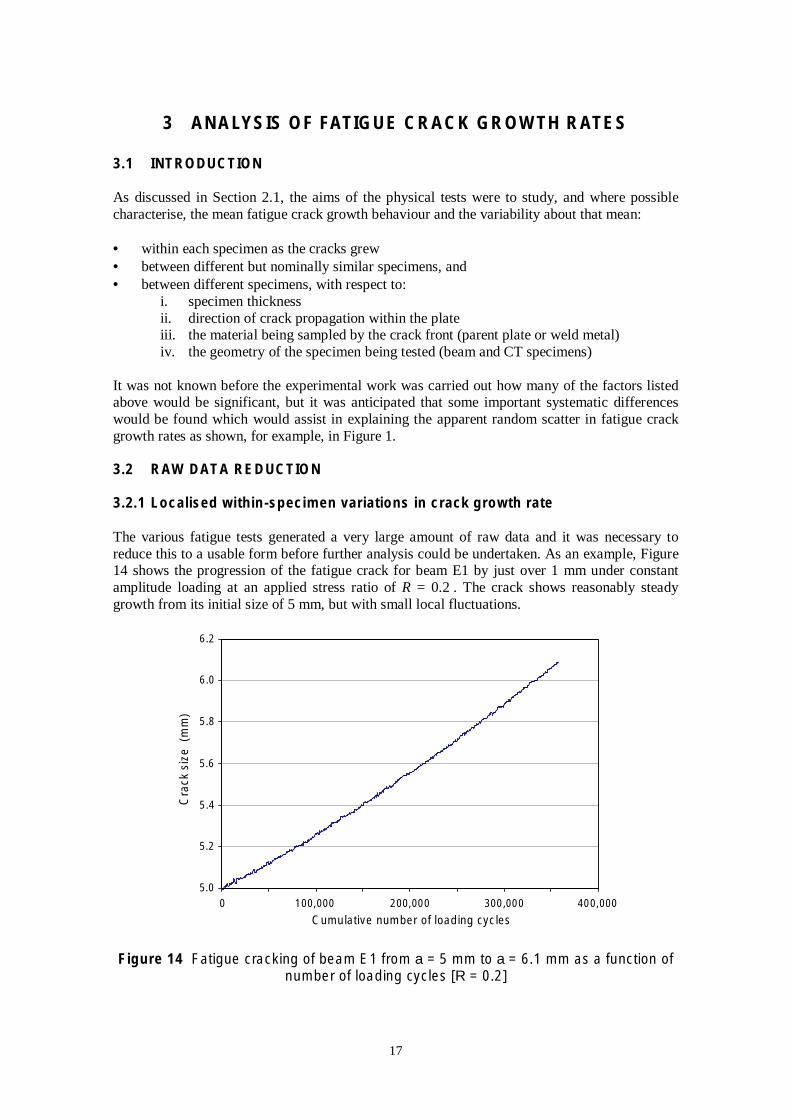
The various fatigue tests generated a very large amount of raw data and it was necessary to reduce this to a usable form before further analysis could be undertaken. As an example, Figure 14 shows the progression of the fatigue crack for beam E1 by just over 1 mm under constant amplitude loading at an applied stress ratio of R = 0.2 . The crack shows reasonably steady growth from its initial size of 5 mm, but with small local fluctuations.

5.0

5.2

5.4

5.6

5.8

6.0

6.2

Cra

ck s

ize

(mm

)

0 100,000 200,000 300,000 400,000

Cumulative number of loading cycles

Figure 14 Fatigue cracking of beam E1 from a = 5 mm to a = 6.1 mm as a function of number of loading cycles [R = 0.2]

17

The crack size was re-measured after approximately every 320 load cycles and typical results can be seen in more detail in Figures 15 and 16 for growth from 8.0-8.1 mm and 15.0-15.1 mm respectively. At these larger scales the crack growth can be seen to be more variable, with periods when the crack is hardly growing and other periods when it is growing more rapidly than average. In Figure 15 there are short periods when the measured crack size decreases, but these are due to random fluctuations in the last significant digit of the ACPD readings. The data were smoothed by using a five-point moving average over all the readings to reduce this effect.

i

10.00

10.02

10.04

10.06

10.08

10.10

925,000 930,000 935,000 940,000

Cra

ck s

ze (

mm

)



i

15.00

15.02

15.04

15.06

15.08

15.10

Cra

ck s

ze (

mm

)

1,270,000 1,275,000 1,280,000



The procedure described above was carried out for all test specimens. In addition, da/dN was plotted against ΔK for the raw data in order to examine any trends, as illustrated in Figure 17 for beam E1. The large amount of scatter arises from the fact that the growth rate was evaluated over successive blocks of only 320 cycles of loading, showing that the measured growth rate was highly variable when averaged over such short time periods (small numbers of loading cycles).

18

19

1.E-06

1.E-05

1.E-04

1.E-03

100 10,0001,000

ΔK (Nmm-3/2)

da/d

N (

mm

/cyc

le)

Figure 17 Computed crack growth rate as a function of ΔK for beam E1, using raw experimental data (in increments of 320 loading cycles). [The banding at lower values

of da/dN is caused by the ACPD output being limited to 4 decimal digits]

0.00

0.01

0.02

0.03

0.04

0.05

0.06

0.07

1 11 21 31 410.00

0.01

0.02

0.03

0.04

0.05

0.06

0.07

1 11 21 31 41

0.00

0.01

0.02

0.03

0.04

0.05

0.06

0.07

1 11 21 31 410.00

0.01

0.02

0.03

0.04

0.05

0.06

0.07

1 11 21 31 41

At ΔK = 400 Nmm-3/2 At ΔK = 600 Nmm-3/2

At ΔK = 800 Nmm-3/2 At ΔK = 1000 Nmm-3/2

Δa (

mm

)

Δa (

mm

)

Δa (

mm

)

Δa (

mm

)

Number of sets of load cycles

Number of sets of load cycles Number of sets of load cycles

Number of sets of load cycles

(a) (b)

(c) (d)

Figure 18 Successive increments of crack extension Δa, over 50 blocks each of 320 load cycles, for four different values of ΔK, corresponding to crack depths of

approximately 14 mm, 29 mm, 40 mm and 48 mm [Beam E1]

The extent of the variability in crack growth rate shown in Figure 17 is difficult to interpet because of the logarithmic scales used in this conventional da/dN versus ΔK plot. The figure appears to show the scatter in da/dN decreasing as the crack grows (ΔK increases), but this is not in fact the case.

To investigate this in more detail, the incremental change in crack size between measurements (i.e. about every 320 cycles of applied load) was studied over the full range of ΔK. Figure 18 shows data for four different stages of the life, corresponding to crack depths of about 14 mm, 29 mm, 40 mm and 48 mm. In Figure 18(a) the increments of crack growth are small and irregular, with no growth occurring in some blocks of load cycles. At the other extreme, Figure

/18(d) gives the same information for a ≈ 48 mm ( ΔK ≈ 1000 Nmm-3 2). In the latter, the average crack growth for each block of 320 load cycles is clearly much larger, as would be expected, but the absolute variability between blocks of cycles is also much larger as well.

This variability in crack growth rate for the beam specimens has been investigated further by computing the sample coefficient of variation (COV) in crack growth rate (defined as the ratio of the sample standard deviation to sample mean) for sets of eight consecutive observations of da/dN each determined over 320 cycles of loading (i.e. over 8×320 = 2560 cycles). These sets were chosen to cover the complete range of crack size (i.e. the complete range of ΔK), and were spaced at intervals of 0.1 mm of crack extension. The results are shown in Figures 19 and 20.

0

20

40

80

100

120

160

ii

ion

of d

a/dN

60

140

Coe

ffic

ent

of v

arat

(%

)

0 500 1,000 1,500 2,000 2,500 /2)ΔK (Nmm-3

Figure 19 Reduction in coefficient of variation of da/dN with ΔK [beam E1]

Coe

ffici

ent o

f var

iatio

n of

da/

dN (

%) 300

100

10

1

100 1000 4000 /2)ΔK (Nmm-3

ion in coefficient of variation of da/dN with ΔKFigure 20 Reductplotted on logarithmic scales [beam E1]

20

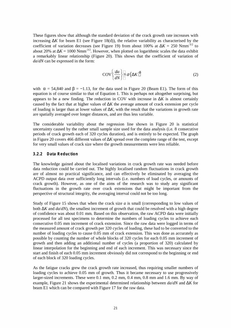
These figures show that although the standard deviation of the crack growth rate increases with increasing ΔK for beam E1 (see Figure 18(d)), the relative variability as characterised by the

/2coefficient of variation decreases (see Figure 19) from about 100% at ΔK = 250 Nmm-3 to /about 20% at ΔK = 1000 Nmm-3 2. However, when plotted on logarithmic scales the data exhibit

a remarkably linear relationship (Figure 20). This shows that the coefficient of variation of da/dN can be expressed in the form:

da βCOV =α (ΔK ) (2)

dN

with α = 54,840 and β = −1.13, for the data used in Figure 20 (Beam E1). The form of this equation is of course similar to that of Equation 1. This is perhaps not altogether surprising, but appears to be a new finding. The reduction in COV with increase in ΔK is almost certainly caused by the fact that at higher values of ΔK the average amount of crack extension per cycle of loading is larger than at lower values of ΔK, with the result that the variations in growth rate are spatially averaged over longer distances, and are thus less variable.

The considerable variability about the regression line shown in Figure 20 is statistical uncertainty caused by the rather small sample size used for the data analysis (i.e. 8 consecutive periods of crack growth each of 320 cycles duration), and is entirely to be expected. The graph in Figure 20 covers 466 different values of ΔK spread over the complete range of the test, except for very small values of crack size where the growth measurements were less reliable.

3.2.2 Data Reduction

The knowledge gained about the localised variations in crack growth rate was needed before data reduction could be carried out. The highly localised random fluctuations in crack growth are of almost no practical significance, and can effectively be eliminated by averaging the ACPD output data over sufficiently long intervals (i.e. numbers of load cycles, or amounts of crack growth). However, as one of the aims of the research was to study any significant fluctuations in the growth rate over crack extensions that might be important from the perspective of structural integrity, the averaging interval could not be too long.

Study of Figure 15 shows that when the crack size a is small (corresponding to low values of both ΔK and da/dN), the smallest increment of growth that could be resolved with a high degree of confidence was about 0.01 mm. Based on this observation, the raw ACPD data were initially processed for all test specimens to determine the numbers of loading cycles to achieve each consecutive 0.05 mm increment of crack extension. Since the raw data were logged in terms of the measured amount of crack growth per 320 cycles of loading, these had to be converted to the number of loading cycles to cause 0.05 mm of crack extension. This was done as accurately as possible by counting the number of whole blocks of 320 cycles for each 0.05 mm increment of growth and then adding an additional number of cycles (a proportion of 320) calculated by linear interpolation for the beginning and end of each increment. This was necessary since the start and finish of each 0.05 mm increment obviously did not correspond to the beginning or end of each block of 320 loading cycles.

As the fatigue cracks grew the crack growth rate increased, thus requiring smaller numbers of loading cycles to achieve 0.05 mm of growth. Thus it became necessary to use progressively larger-sized increments. These were 0.1 mm, 0.2 mm, 0.4 mm, 0.8 mm and 1.6 mm. By way of example, Figure 21 shows the experimental determined relationship between da/dN and ΔK for beam E1 which can be compared with Figure 17 for the raw data.

21

1.E-03

da/d

N (

mm

/cyc

le)

1.E-04

1.E-05

1.E-06

100 1,000 10,000

/2)ΔK (Nmm-3

Figure 21 Observed fatigue crack growth relationship for beam E1 based on crack increments of 0.4 mm, 0.8 mm and 1.6mm

The final stage in the data reduction process was then to fit a suitable ‘smooth’ curve to the experimental data for each test specimen, to enable comparisons between specimens to be easily made without the need to include all the experimental data, for example between welded and non-welded beams. This is illustrated in Figure 22 for beam E1. Similar plots, giving the reduced data for all the test specimens are included in Appendices 1-4.

//

l

l ial it

1.E-06

1.E-05

1.E-04

1.E-03

dadN

(m

mcy

ce)

4th order po ynom curve f

100 1000 10000 /2)ΔK (Nmm-3

Figure 22 4th order polynomial fit to experimental data for beam E1

22

3.3 ANALYSIS OF NON-WELDED BEAM SPECIMENS

3.3.1 Introduction

The results of the experimental test programme are discussed in Sections 3.3 to 3.6 for the four main groups of test specimens, namely non-welded beams, welded beams, non-welded CT specimens and welded CT specimens, respectively. It should be recalled that the locations of the various test specimens are shown in Figure 6. The plots of the reduced da/dN versus ΔK data are given for each specimen in Appendices 1-4, together with testing details such as the maximum and minimum values of the applied load (Pmax and Pmin) in Tables A1-A4 of these appendices. The approach adopted will be the same for each group, namely a commentary on each of the individual tests will be followed by comparisons between tests within each group. Finally, comparisons will be made on the differences in fatigue behaviour between each of the four groups.

3.3.2 Non-welded beam specimens

In total four non-welded beams were tested, two with the crack propagating up through the thickness of the plate (B2 and E2) and two with the crack propagating across the plate (B1 and E1). Beam E1 was 100 mm deep, which was twice the depth of the other three beams. As previously shown in Figure 21 (also Figure A1), beam E1 exhibited a relatively smooth, but

/non-linear, crack growth curve starting at a low value of ΔK ≈ 247 Nmm-3 2, and corresponding to an initial extreme fibre bending stress at mid span of 75 Nmm-2. As explained in Section 3.3.2, the increments of ΔK shown on the horizontal axes of these graphs correspond to increments of crack growth Δa of 0.4 mm, increasing to 0.8 mm as the growth rate increases at larger crack sizes.

Beam specimen E2 was cut from a piece of plate physically adjacent to beam E1 but was orientated so that the fatigue crack propagated up through the plate. The test had to be carried at a higher applied bending stress (144 Nmm-2) than beam E1 because of the beam’s significant resistance to fatigue crack growth at lower loads. As a result the crack growth curve starts at a

/higher applied value of ΔK ≈ 470 Nmm-3 2, as shown in Figure A2. This higher resistance to fatigue cracking was likely to have been due to compressive residual stresses in the outer layers of the beam resulting from rolling, thus reducing the effective stress ratio.

Comparison of Figures A1 and A2 shows that there is an order of magnitude more variability in the growth rate for the crack propagating in the through-thickness direction than for the crack growing across the plate, and that in beam E2 the variability is particularly marked as the crack grows through the central region of the plate. The two figures give directly comparable information since the growth rates for the two beams were calculated over the same increments of crack growth (namely 0.4 mm and then 0.8 mm) and in both cases the length of the crack front was 50 mm. This difference in variability is almost certainly due to inherent through-thickness variability in steel microstructure, originating from the steel production and rolling processes. As the crack in beam E2 grows through the thickness of the plate, the whole crack front would have been sampling roughly similar microstructure at each value of crack depth. In contrast, in beam E1 the crack front samples the complete cross-section of the plate throughout the test, thus effectively averaging the through-thickness properties at each moment in time (i.e. each position of the crack front). This has resulted in a much lower variability in crack growth rate than for beam E1.

Turning now to beams B1 and B2 (see Figure 6), these were initially adjacent pieces of plate, but from a different region than test pieces E1 and E2. The crack growth rates for B1 and B2 are

23

shown in Figures A3 and A4 respectively. Beam B2, in which the direction of fatigue cracking was the same as that for beam E2, shows greater variability in growth rate than beam B1, although this is not as marked as in beam E2.

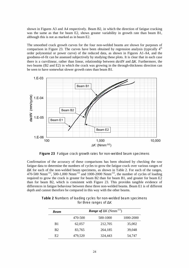
The smoothed crack growth curves for the four non-welded beams are shown for purposes of comparison in Figure 23. The curves have been obtained by regression analysis (typically 4th

order polynomial or power curve) of the reduced data, as shown in Figures A1-A4, and the goodness-of-fit can be assessed subjectively by studying these plots. It is clear that in each case there is a curvilinear, rather than linear, relationship between da/dN and ΔK. Furthermore, the two beams (B2 and E2) in which the crack was growing in the through-thickness direction can be seen to have somewhat slower growth rates than beam B1.

1.E03

1.E04

1.E05

1.E06

Beam B1

Beam B2

Beam E1

Beam E2

100 1,000 10,000 K )(Nmm 3/2

Figure 23 Fatigue crack growth rates for non-welded beam specimens

Confirmation of the accuracy of these comparisons has been obtained by checking the raw fatigue data to determine the numbers of cycles to grow the fatigue crack over various ranges of ΔK for each of the non-welded beam specimens, as shown in Table 2. For each of the ranges,

/ / /470-500 Nmm-3 2, 500-1,000 Nmm-3 2 and 1000-2000 Nmm-3 2, the number of cycles of loading required to grow the crack is greater for beam B2 than for beam B1, and greater for beam E2 than for beam B2, which is consistent with Figure 23. This provides tangible evidence of differences in fatigue behaviour between these three non-welded beams. Beam E1 is of different depth and cannot therefore be compared in this way with the other beams.

Table 2 Numbers of loading cycles for non-welded beam specimens for three ranges of ΔK

Beam Range of ΔK (Nmm -3/2)

470-500 500-1000 1000-2000

B1 62,057 212,705 35,002

B2 83,765 264,185 39,048

E2 479,520 324,443 54,747

24

3.4 ANALYSIS OF WELDED BEAM SPECIMENS

Test results are available for only two of the three welded beam specimens, namely A1a and A2, because of difficulties in crack growth measurement for test A1b. However, beams A1a and A2 were tested under the same loading regime, details of which are given in Table A2. For beam A1a, the fatigue crack grew upwards through the weld metal from the lower surface of the plate to the top; and for beam A2 the crack grew across the plate in the direction of welding, also in the weld metal (see Figure 6).

The detailed crack growth data for these two beams are shown in Figures A5 and A6 (Appendix 2), and these results can be compared with each other and with the non-welded beams in Figure 24 below. Over a large range of ΔK, the growth rates for beam A1a are significantly higher than for A2, with the results for the two beams lying respectively above and below those of the non-welded specimens. Beam A2 shows considerably enhanced overall fatigue properties in comparison with any of the other beams, although there is a reasonably high degree of local scatter in the growth rate (Figure A6).

i lFigure 24 Fat gue crack growth rates for we ded beam specimens

For beam A1a the crack front remained reasonably straight, and parallel to the initial notch, throughout the test. However, for beam A2 it developed an irregular shape with slower growth in the central region than in the upper and lower regions of the weld. This shape is consistent with welding-induced compressive residual stresses being present at the root of the weld in the centre of the beam, these being balanced by self-equilibriating tensile residual stresses in the upper and lower parts of the weld (see diagram of Beam A2 in Figure 11). The fatigue and fracture surfaces for the two beams are shown in Figures 25(a) and 25(b) respectively. It should be noted that because of the different directions of crack growth, the top and bottom surfaces of the plate are at the top and bottom of Figure 25(a), but on the left and right of Figure 25(b). It can be seen that there was a severe root defect in Beam A2, but this is likely to have had little influence on the rate of crack propagation because it was at right angles to the direction of crack propagation.

25

Figure 25(a) Beach Marking Figure 25(b) Beach Marking Beam A1a Beam A2

The irregular crack front in Beam A2 makes the determination of the stress intensity factors difficult. However, these were calculated by assuming a linear crack front with a crack depth equal to the average of the three ACPD channels. The extent to which this approach is reasonable can be judged by comparing the total numbers of loading cycles required to drive the crack forward for the two beams. This information is given in Table 3. It can be seen that for each of the four ranges of ΔK selected, the total number of loading cycles required to propagate the crack is considerably more for Beam A2 than for Beam A1a. Furthermore, the total numbers of cycles from crack initiation to failure were 481,000 and 2,897,630 for beams A1a and A2 respectively, a difference of a factor of six. This confirms that the relative position of Beams A1a and A2 on Figure 24 are correct, and indeed that they lie above and below the curves for the non-welded beams.

Table 3 Numbers of loading cycles for beam specimens A1a and A2 for three ranges of ΔK

Beam Range of ΔK (Nmm -3/2)

400-470 470-500 500-1000 1000-2000

A1a 163,644 30,083 115,952 77,215

A2 482,827 143,886 1,434,711 191,237

3.5 ANALYSIS OF NON-WELDED COMPACT TENSION SPECIMENS

The total number of non-welded compact tension specimens tested was 11 and the crack growth rates for these are shown in Figures A7 to A28 (Appendix 3). Test details are shown in Table A3. The tests comprised six large specimens with dimension W = 100 mm and five smaller specimens with W = 40 mm. As explained previously and as shown in Figure 6, the larger specimens, denoted Hz, were machined from the plate in such a way that that their largest side was parallel to the original plate surface. The smaller specimens, denoted Vz, were prepared by making vertical cuts through the plate.

26

For each test specimen the crack growth rates are presented in two graphs (e.g. Figures A7 and A8 for specimen Hz D1), the first using rates averaged over minimum increments of crack extension of 0.05 mm, and the second with minimum increments of 0.4 mm. For both graphs, larger increments of 0.8 mm and 1.6 mm are used for the higher values of ΔK because of the relative sparseness of data when the crack is growing relatively quickly.

The reason for providing two plots for each specimen is to be able to distinguish between the rapid fluctuations in growth rate that occur over very small crack extensions and the more slowly varying trends. As with the beam tests, the values of ΔK shown in Figures A7 to A28 correspond to increments of crack extension of either 0.05 mm or 0.4 mm for the lower and medium values of ΔK. It is obvious that when the growth rate is averaged over the larger increment of 0.4 mm, the more rapid fluctuations will be averaged out and the variability about the mean curve will be reduced.

The results for specimen Hz D1 are shown in Figures A7 and A8 and are reasonably typical of many of the CT specimens. Hz D1 is a full-plate thickness specimen (t = 50 mm) and shows moderate variability in growth rate over increments of crack extension of 0.05 mm, which is reduced when the increments are increased to 0.4 mm. The crack growth curve is somewhat sigmoidal in shape, but is reasonably linear over most of the range of ΔK.

Hz D2-1 and Hz D2-2 (Figures A9 to A12) are nominally half plate thickness specimens (t = 21.9 mm) tested under the same loading regime. For Hz D2-1, it is noticeable that about 1.5 mm of measured crack growth is required before the growth curve becomes linear, whereas for Hz D2-2 the growth curve is linear from the start. It is likely that for Hz D2-1 the initial overall crack growth rate is slower because the crack initiation along the crack front may not have been co-planar for the multiple initiation sites, with the result that a certain amount of growth was required for a planar crack to be fully developed. This characteristic is exhibited by a number of test pieces.

Hz D3-1, Hz D3-2 and Hz D3-3 (Figures A13 to A18) are three of four nominally quarter plate thickness specimens (t = 8.1 mm). The fourth, Hz D3-4, was damaged by an accidental overload during testing. What is immediately noticeable from these results is that there is much greater variability in the observed growth rate about the mean curves than for the thicker specimens. There are two possible explanations for this. The first is that the crack growth rate at each position on the crack front is indeed less variable for the thicker specimens because of physical constraint on the crack. The second is that local variations in crack extension along the crack front are being spatially averaged in the ACPD measurements, with the result that the observed variance is smaller. It seems likely that both of these effects are taking place.

A further observation is that the variability in crack growth rate is larger for the specimens cut from the centre of the plate than from near the plate surface, as can be seen by comparing Figures A15 and A17 with Figure A13, or Figures A16 and A18 with Figure A14. This is likely to be due to the outer regions of the plate having a more refined microstructure.

As previously stated, the highly localised variability in fatigue crack growth rate is of little practical significance except in as much as it interferes with the measurement of the mean crack growth characteristics, making this more difficult. However, this is of practical importance for in-service monitoring and inspection. As illustrated in Sections 3.4 and 3.5, it is the differences between the mean crack growth curves that are of importance in governing fatigue life. A comparison of these for the non-welded Hz CT specimens is made in Figure 26 below. Only the linear part of the da/dN versus ΔK relationship is shown in each case, but for these specimens there was little deviation from linearity as discussed above.

27

//

l

1.E-06

1.E-05

1.E-04

1.E-03

1.E-02

Hz D3-1 (8.1mm)

Hz D3-3 (8.1mm)

Hz D3-2 (8.1mm) Hz D2-1 (21.9mm)

Hz D1 (50mm)

dadN

(m

mcy

ce)

Hz D2-2 (21.9mm)

100 1,000 10,000

/2)ΔK (Nmm-3

Figure 26 Fatigue crack growth rates for non-welded CT specimens (Hz)

//

l

1.E-06

1.E-05

1.E-04

1.E-03

1.E-02

Vz E3-3 (5mm)

Vz E2-2 (10mm)

Vz E3-1 (5mm)

Vz E3-2 (10mm)

Vz E2-2 (10mm)

Vz E1 (20mm)

Vz E3-2 (10mm)

Vz E1 (20mm)

dadN

(m

mcy

ce)

100 1,000 10,000

/2)ΔK (Nmm-3

Figure 27 Fatigue crack growth rates for non-welded CT specimens (Vz)

28

Figure 26 shows up some significant differences, with the three thinnest specimens having lower growth rates than the other Hz CT specimens. So although these thinner specimens exhibited more localised variability, their overall fatigue performance was superior. Continuing this trend, specimen Hz D1 which was 50 mm thick is seen to have the fastest crack growth of all six Hz specimens.

Turning now to the five smaller Vz specimens (see Figure 6), the detailed results for these are shown in Figures A19 to A28. These have not dissimilar characteristics to the Hz specimens, with greater local variability exhibited when the growth rate is determined over 0.05 mm crack increments, as would be expected. With one exception, namely Vz E3-2, all the crack growth curves can be taken to be linear. Comparison of these mean curves is made in Figure 27, from which it can be seen that they are all closely similar. In contrast to the Hz specimens there appears to be no significant thickness effect in relation to the mean curves, with the results for the five specimens being tightly grouped. For the 5 mm thick specimens Vz E3-1, Vz E3-2 and Vz E3-3 there is some evidence that crack growth curve is approximately bi-linear, with the

/lines becoming less steep at values of ΔK greater than about 900 Nmm-3 2, but otherwise the classic linear da/dN versus ΔK relationship appears to be the best model for values of ΔK in the mid-range of stress intensity.

i ll lFigure 28 Fat gue crack growth rates for a non-we ded CT specimens (Hz and Vz) compared with design limits from Figure 3 based on King (1998)

(Vz specimens are shown with a broken line)

Finally, Figure 28 compares the crack growth rates for the Hz and Vz non-welded CT specimens. There are no significant differences between the two groups, except for the fact that the Vz curves are less variable. This is perhaps not surprising, since all the Vz specimens were physically adjacent to each other in the original plate (Figure 6). Nevertheless, the differences that exist correspond to not insignificant differences in fatigue life. In addition, Figure 28

29

compares the experimental data for CT specimens with the mean plus two standard deviation design curve proposed by King (1998), as plotted in Figure 3. Whilst most of the experimentally-based crack growth curves lie within the plus and minus two standard deviation limits, specimens Hz D1 and Vz E3-3 have higher growth rates than the design curve for values

/ /of ΔK greater than 700 Nmm-3 2 and 1000 Nmm-3 2 respectively. In addition, specimen Hz D2-1 lies almost exactly on the design curve.

3.6 ANALYSIS OF WELDED COMPACT TENSION SPECIMENS

The reduced crack growth data for the 13 welded CT specimens are given in Figures A29 to A54 of Appendix 4 and the corresponding test details are summarised in Table A4. As with the non-welded CT specimens, two graphs of da/dN versus ΔK are included for each test, the first based on 0.05 mm increments of crack growth and the second on 0.4 mm increments. Figures A29 to A42 give the test data for the larger size Hz specimens C1 to C3-4, and Figures A43 to A54 are for the smaller Vz specimens. For all the welded Hz specimens the direction of crack propagation was in the direction of welding (i.e. along the weld), whilst for the Vz specimens, the fatigue crack grew up from the bottom surface of the plate through the weld (see Figure 6).

Hz C1 was a 50mm thick specimen and as can be seen in Figures A29 and A30 exhibited a relatively small amount of localised variability in growth rate, even for 0.05 mm increments of crack extension. The overall da/dN versus ΔK relationship was sigmoidal in shape with a much steeper gradient than the equivalent non-welded specimen Hz D1 (Figure A8).

For the half plate thickness specimens Hz C2-1, there was again very little localised variability in growth rate, but the overall da/dN versus ΔK curve was extremely steep for the first 10 mm of crack extension, before reducing and then rising again steeply as shown in Figure A32. This anomaly is likely to have been caused by the fatigue crack sampling a part through-thickness weld defect. Hz C2-2 (Figure A34) shows somewhat similar characteristics, but with greater localised variability in the early stages of crack propagation.

The four quarter plate thickness specimens C3-1 to C3-4 (with t = 8.1 mm) all exhibit very similar behaviour, with a relatively steep but linear crack growth relationships (see Figures A35 to A42). However, each shows a relatively large amount of local variability in growth rate, as compared to the thicker specimens.

To compare all the welded Hz specimens, the smoothed crack growth curves are plotted in Figure 29 below. It can be seen that the four nominally similar 8.1 mm thick specimens have very similar crack growth curves. However, the thickness effect noticed for the non-welded specimens is also present with the thickest specimen Hz C1 having growth rates approximately an order of magnitude higher than the 8.1 mm thick specimens. Specimen Hz C2-2 which is 21.9 mm thick is in an intermediate position.

The last set of results to be considered are for the smaller vertical Vz specimens, Vz C4 to Vz C10 (see Figure 6). Compared with the Hz specimens these specimens exhibit a relatively large amount of localised variability in crack growth rate, even for the thicker specimens (t = 20 mm and t = 10 mm), as shown in Figures A43, A45 and A47. However, when averaged over 0.4 mm of crack extension relatively smooth crack growth relationships are found (Figures A44, A46 and A48). For the thinnest specimens, Vz C7, Vz C9 and C10 (with t = 5 mm), each shows somewhat different characteristics, which is probably a result of local differences in the weld characteristics, even though the specimens were adjacent to each other.

30

//

l

1.E-06

1.E-05

1.E-04

1.E-03

1.E-02

Hz C1 (50mm)

Hz C3-1 (8.1mm)

Hz C3-2 (8.1mm)

Hz C3-4 (8.1mm)

Hz C3-3 (8.1mm)

Hz C2-2 (21.9mm)

dadN

(m

mcy

ce)

100 1,000 10,000

/2)ΔK (Nmm-3

Figure 29 Fatigue crack growth rates for welded CT specimens (Hz)

As with the previous data sets, all the results for the welded Vz CT specimens have been plotted on the same graph (Figure 30) which shows a wide range of different behaviour, but with specimens C9 and C10 which were tested under identical conditions being very similar. Specimen C7 which also has a thickness of 5 mm but which was tested at a lower value of Pmax

has a much steeper characteristic. Specimen Vz C6, with a thickness of t = 10 mm, was the most fatigue resistant, as shown in Figure 30. As discussed earlier in relation to the beam tests, the validity of this finding has been confirmed by comparing the total number of cycles to failure of specimens Vz C5 and Vz C6. In all other respects these specimens were nominally identical, including the loading regime. This illustrates that large differences in overall crack growth rate can occur between nominally similar specimens in the case of cracks propagating in weld metal.

Finally, Figure 31 provides a comparison between the welded Hz and Vz specimens. For non-welded specimens there were no discernable differences between the fatigue behaviour of the two types (see Figure 31), but for the welded specimens the Hz specimens have noticeably steeper growth characteristics. This means that the cracks start growing at much lower rate than the Vz specimens, although they have superior fatigue performance at low values of ΔK, i.e. when the fatigue crack is growing in the direction of welding. However, the growth rate increases much more rapidly, and in most cases exceeds that of the Vz specimens.

Figure 31 also shows the fatigue design line at mean plus two standard deviations based on the data analysed by King (1998). It can be seen that many of the crack growth curves for these welded specimens fall well below the design line, and indeed well below the mean minus two standard deviation line, showing that the welded steel specimens have relatively superior fatigue properties in comparison with those of the parent plate. However, there are very wide variations.

31

//

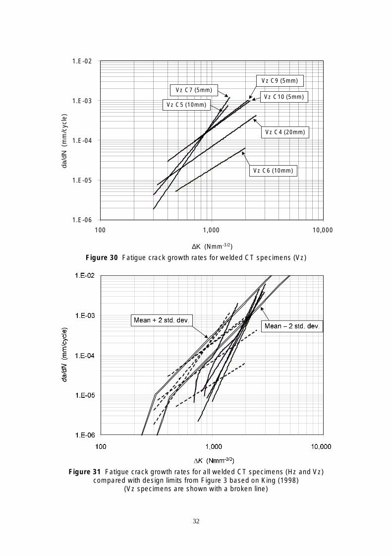
l

1.E-06

1.E-05

1.E-04

1.E-03

1.E-02

Vz C5 (10mm)

Vz C7 (5mm)

Vz C4 (20mm)

Vz C9 (5mm)

Vz C10 (5mm)

Vz C6 (10mm)

dadN

(m

mcy

ce)

100 1,000 10,000

/2)ΔK (Nmm-3

Figure 30 Fatigue crack growth rates for welded CT specimens (Vz)

i ll lFigure 31 Fat gue crack growth rates for a we ded CT specimens (Hz and Vz) compared with design limits from Figure 3 based on King (1998)

(Vz specimens are shown with a broken line)

32

4 INTERPRETATION OF EXPERIMENTAL FINDINGS

4.1 INTRODUCTION

The detailed results of the experimental programme have been given in Section 3 above and in Appendices 1-4. The principal findings are discussed here.

4.2 WITHIN AND BETWEEN SPECIMEN VARIABILITY IN FATIGUE CRACK GROWTH RATES

As discussed in Section 2, fatigue crack growth rates for carbon steels exhibit large amounts of variability even when plotted on logarithmic scales. It is not generally known, however, how much of this is due to short-duration random fluctuations and how much is due to systematic differences which affect the mean crack growth curve. Before this experimental work, it was also not known how the short-term fluctuations are affected by factors such as crack length, specimen thickness and basic material properties. Knowledge of these effects is clearly important in the fatigue crack monitoring of real structures, since a high observed growth rate over a short period of time might indicate a high mean rate or may be just a high short-term fluctuation.

Figure 5 based on data from Virkler et al (1978) shows that for thin aluminium alloy panels the crack growth rate can fluctuate significantly during a test at constant stress range. Somewhat similar effects have been observed in the present work, as shown in Figure 15, but the fluctuations here take place over very small crack extensions (and correspondingly small changes in ΔK) and the very high variability shown in Figure 17, where the crack growth has been recorded in increments of only 320 loading cycles, averages out to give a relatively smooth curve when the growth is measured over successive increments of 0.4 mm or more (Figure 21). This finding holds for all the specimens tested and is a well-known phenomenon which is recognised in standards for fatigue testing. However, for the work reported here, the mean

/(smoothed) da dN versus ΔK relationships were found to deviate significantly from a straight line on a log-log plot for many of the test specimens, as discussed in Sections 4.2.3 and 4.2.4.

4.2.1 Short-term variability in fatigue crack growth in the parent plate

The term short-term variability is used here to define fluctuations in crack growth rate over increments of crack extension of less than 0.2 mm, as opposed to the longer term variations in growth rate that can occur over distances of several millimetres or more.

A study of the detailed test data for all the specimens given in Figures A1-A54 (Appendices 1 to 4) shows that the short-term random fluctuations in crack growth rate are influenced by a number of factors. For cracks growing in the parent plate (Appendices 1 and 3), it is clear that the observed growth was less variable for the thicker specimens having a longer crack front, as can be seen, for example, by comparing Figure A7 with Figures A13 or A15 in which the crack growth rate was measured over increments of 0.05 mm. However, as previously noted, it is not clear the extent to which this reduction in variability is the result of constraint on the crack tip in the thicker specimens, or the spatial averaging of the crack depth along the crack front resulting from the ACPD measurement technique used.

A further finding of interest was the difference in the variability of the crack growth rate between specimens cut from the inner part of the plate and from those from nearer the surface, as exhibited by the Hz CT specimens in which the crack was growing across the plate. This can be seen by comparing Figure A13 with Figures A15 and A17 for the 0.05 mm growth

33

increments, and Figure A14 with Figures A16 and A18 for the 0.04 mm increments. This difference in variability can be attributed to differences in microstructure between the inner and outer regions of the plate, with the more refined microstructure in the outer regions giving less variable growth.

For the Vz specimens the fatigue cracks were growing upwards through the thickness of the plate, and most of these exhibited a significant amount of variability in growth rate. As shown in Figure 6, these specimens were physically adjacent to each other and therefore might have been expected to have very similar fatigue characteristics. This is indeed the case for the mean growth curves, as shown in Figure 27. However, in terms of crack growth variability there are some noticeable differences, for example with adjacent and nominally identical specimens E3-2 and E3-3 behaving rather differently (see Figures A25 and A27). It can be concluded that these differences were simply due to localised differences in plate microstructure.

Finally, there is also some evidence from the Vz specimens (e.g. Figures A21, A23 and A27) that the variability in growth rates increases as the fatigue crack grows into the central part of the plate, which supports the findings from the Hz specimens discussed above. The same effect can also be noticed in the beam specimens; with beam E2 in which the crack was growing upwards through the plate showing much more variability than beam B1 where the crack grew in the across-plate direction. Comparison of beams B1 and B2 also shows these differences, but to a lesser extent.

Returning now to the results given in Figures 18 and 19, it was demonstrated for beam specimen E1 that the short-term variability in growth rate (characterised by the standard deviation in crack growth Δa over sets of 320 cycles of loading), increased with ΔK. However the mean crack growth rate increased faster than the standard deviation, with the result that coefficient of variation in da/dN was shown to decrease with ΔK (Figure 20). Similar findings can be expected for the other specimens although these data have not been analysed. This leads to the result given by Equation 2 that the coefficient of variation in crack growth rate representing the short-term variability in da/dN takes the same form as the Paris law, namely

da βCOV =α (ΔK )

dN

and taking logarithms,

log COV

da = log α β log (ΔK ) (3) +

dN

For known values of ΔK, the uncertainty in the COV of da/dN measured over a fixed number of load cycles N can therefore be modelled in terms of two parameters α and β.

4.2.2 Short-term variability in fatigue crack growth in the weld material

For the two welded beams A1a and A2, the short-term variability in growth rate was seen to be significantly greater for the beam in which the crack propagated in the direction of welding (Beam A2). This is likely to have been because of the irregular and changing shape of the crack front which in turn resulted from the root of the weld at the centre of the plate being under a state of high compressive residual stress as a result of the welding process.

For the welded CT specimens, comparison of Figure A29 with Figure A7 shows that for the full-thickness Hz specimens C1 and D1 (where the fatigue cracks were growing along the weld

34

and across the plate respectively) the short-term variability was in fact somewhat less for the welded specimen (C1) than for the non-welded one (D1) but not markedly so. For the half- and quarter-thickness Hz specimens, the welded ones also show less variability as can be seen by comparing Figures A37 and A39 for Hz C3-2 and Hz C3-3 with Figures A15 and A17 for Hz D3-2 and Hz D3-3.

However, for the Vz specimens in which the cracks were growing up through the plate, and with the crack front progressing from weld bead to weld bead, the short-term variability was much greater for the welded specimens than for the otherwise identical non-welded ones (for example compare Figure A43 with A19 and A47 with A21).

A firm conclusion from this investigation therefore is that when the crack front was sampling a cross-section of the weld and intersecting a number of weld runs (as in the Hz specimens), the short-term variability in growth rate was very much lower than when the crack front was parallel to the direction of welding (as in the Vz specimens).

4.2.3 Long-term variability in fatigue crack growth in the parent plate

The two previous sections of this report have considered the short-term fluctuations in crack growth rate. Because these fluctuations tend to average out over moderate amounts of crack extension, they are of relatively little practical importance except in the way in which they make the monitoring of crack growth more difficult in the short term. We now turn to consideration of the more slowly varying trends and how specimen geometry and crack orientation were found to affect these. This section deals with fatigue cracks in the parent plate whereas Section 4.2.4 deals with those in the weld metal.

The main results for non-welded beams and non-welded CT specimens have already been given in Figures 24, 26, 27 and 28. Considering the CT specimens first, it can be concluded that:

/• the crack growth for most of the specimens followed a linear Paris-type log( da dN ) versus log( ΔK) relationship, but with some variation in slope m and position (Figures 26 and 27)

• the thicker specimens tended to fatigue more quickly than those of thinner cross-section (Figure 26)

• the majority of the curves were within the ± two standard deviation limits of the data reported by King (1998), although two specimens showed faster crack growth at high values of ΔK (Figure 28)

• the linear nature of the mean crack growth relationships means that the relatively slow fluctuations reported by Virkler for thin aluminium alloy specimens (Figure 5) were not present

• as one specimen (Hz D2-1) had a growth curve which was practically coincident with the mean + two standard deviation limit reported by King over the complete range of the test, it is clear that this is not particularly conservative as a design curve

• there were no marked differences in the crack growth relationships between the Hz and Vz specimens showing that fatigue cracks growing through the thickness of the plate and across the plate behaved in a similar manner in terms of their long-term growth behaviour, and with approximately the same variability in slope m. The thickest specimen Hz D1, however, showed a higher growth rate than any of the other specimens at values of ΔK

/2greater than 700 Nmm-3 .

A notable experimental finding from this research has been the effect of increased specimen thickness on increasing the average rate of fatigue crack growth. This has been exhibited by many of the groups of specimens. A theoretical explanation for this has been proposed by Tong (2002) and others in terms of the magnitude of the T-stress acting at the crack front.

35

A suggestion has been made by some other researchers that fatigue behaviour is better

characterised by plotting da/dN as a function of Δ J , where J is the J-integral, rather than ΔK. However, a detailed study of both the beam and CT specimens used in this work by 3-d finite element-based J-integral analysis (Nahar Hamid, 2006) has shown that this is not the case.

Turning now to the four non-welded beam specimens, some explanation for the differences found have already been given in Section 3.2.2. All four beams showed curvilinear crack growth relationships extending over the complete range of ΔK, and lying within the ± two

/standard deviation limits reported by King (1998) between ΔK values of 600 Nmm-3 2 and 1,200 /Nmm-3 2. The slower crack growth exhibited by Beam E2, and to a lesser extent by Beam B2 is

almost certainly due to rolling-induced compressive residual stresses in the outer layers of the plate. Although the reported values of ΔK are correct within the limits of experimental error, it is clear that because of the presence of residual stresses Beams E2 and B2 were effectively tested under a regime of changing stress ratio R throughout the two tests, as the residual stresses were slowly released with the growth of the fatigue crack. This could partly account for the relatively rapid increase in da/dN as the fatigue crack grew into the central region of the plate. However, this can only be a partial explanation because of the very similar behaviour shown by Beam B1.

Finally, it can be concluded that: /• the log( da dN ) versus log( ΔK) fatigue crack growth curves were relatively smooth when

averaged over reasonably large increments of crack growth (i.e. 0.4 mm) • even within the non-welded regions of the plate, significant differences in fatigue crack

growth rate have been demonstrated for given values of ΔK • these differences are corroborated by significant differences in overall fatigue life during

testing (i.e. numbers of cycles to failure under the same constant amplitude loading) • some of the differences can be explained in terms of physical differences such as specimen

thickness and the presence of rolling-induced residual stresses • the remaining differences are of a random nature and lead to random variations in slope

and position of the crack growth curve for specimens which are in all other respects nominally identical.

4.2.4 Long-term variability in fatigue crack growth in the weld material

Starting with the two welded beam specimens A1a and A2 (Figures A5 and A6 in Appendix 2), these differ in fatigue life by a factor of 6, with A2 being the most fatigue resistant. For A2 the crack grew down the length of the weld simultaneously sampling a number of weld beads and zones with a range of compressive and tensile residual welding stresses, but this nevertheless resulted in a highly fatigue resistant specimen as previously shown in Figure 24. Beam A1a on the other hand, in which the fatigue crack was growing in an orthogonal direction, was the least fatigue resistant of the beam specimens, but this can be accounted for by high tensile residual stresses in the early stage of the test which would have resulted in a high R value.

Turning now to the welded CT specimens, it has previously been seen that whereas for the non-welded test pieces there were no significant differences between the Hz and Vz directions (see Figure 28), for the welded test pieces those cut in the Hz direction (with the fatigue crack running along the weld) performed in a superior manner with longer fatigue lives (see Figure 31). However, the Hz specimens exhibited much steeper gradients showing a faster increase in crack growth rate than those of the Vz type. Since there were no other differences between the welded and the non-welded CT specimens, the effects here must clearly be a result of the welding.

36

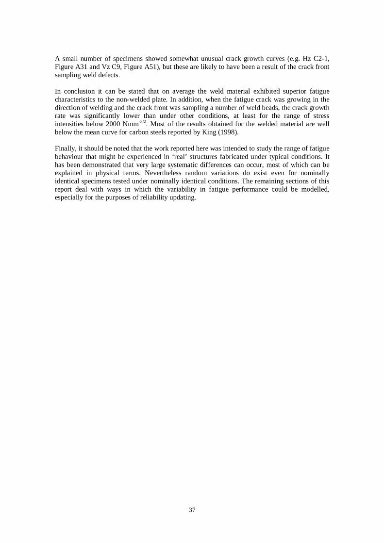
A small number of specimens showed somewhat unusual crack growth curves (e.g. Hz C2-1, Figure A31 and Vz C9, Figure A51), but these are likely to have been a result of the crack front sampling weld defects.

In conclusion it can be stated that on average the weld material exhibited superior fatigue characteristics to the non-welded plate. In addition, when the fatigue crack was growing in the direction of welding and the crack front was sampling a number of weld beads, the crack growth rate was significantly lower than under other conditions, at least for the range of stress

/intensities below 2000 Nmm-3 2. Most of the results obtained for the welded material are well below the mean curve for carbon steels reported by King (1998).

Finally, it should be noted that the work reported here was intended to study the range of fatigue behaviour that might be experienced in ‘real’ structures fabricated under typical conditions. It has been demonstrated that very large systematic differences can occur, most of which can be explained in physical terms. Nevertheless random variations do exist even for nominally identical specimens tested under nominally identical conditions. The remaining sections of this report deal with ways in which the variability in fatigue performance could be modelled, especially for the purposes of reliability updating.

37

5 DEVELOPMENT OF STOCHASTIC FATIGUE CRACK GROWTH MODELS

5.1 INTRODUCTION

Any procedure for predicting the reliability of a structure requires at least two components – an underlying mathematical model of the physical failure process (the, so-called physical or mechanical model) and related stochastic or probabilistic models for the uncertainties in the parameters of the physical model (Thoft-Christensen and Baker, 1982). These two types of model are generally not unrelated because any simplifications that are introduced into the physical modelling of the failure process must be compensated by an increase in model uncertainty and possibly in the uncertainties in the parameters that characterise that model. This is especially the case when the physical model is wholly or partly empirical, which is the case with fatigue failure.

In predicting the fatigue life of a structure or component, the normal approach during design or assessment is to determine conservative (i.e. pessimistic) estimates of the remaining time, or number of loading cycles, to failure. In a traditional deterministic approach this is done simply by using what are judged to be suitably conservative values of all the design parameters (generally obtained from codes of practice, e.g. BS7910). However, in a reliability-based approach it is possible to determine values of the remaining fatigue life that have any specified probability of being exceeded (e.g. 50%, 95%, 99.999%, etc), and from which better risk-based decisions can often be made. This may be particularly useful if the consequences of failure are likely to be severe. Alternatively one may calculate the probabilities that the structure will survive without fatigue failure for specified further periods of time (e.g. 10, 20 or 50 years).

The calculations described above (whether deterministic or probabilistic) may be performed at the design stage before the structure is built, or at any time during the structure’s life. However, unless new information on the current state of the structure is used during this process, the calculations will obviously produce the same results, which is not very useful. If, however, information can be gained on the fatigue performance of the structure at various times during its life, the information available up to the time at which the assessment, or re-assessment, is made can be used to improve the prediction of the remaining fatigue life – i.e. to reduce the variance in its predicted value.

As shown both by experiment and industrial experience, the fatigue lives of nominally similar structures can vary significantly, so (even without calculation) it is not unreasonable to suggest that structures containing defects that are showing no signs of fatigue cracking, or where the cracks are growing more slowly than might be expected, will have longer fatigue lives than those in which fatigue cracks have been observed to be growing at a faster rate. This is intuitively obvious. However, one of the uncertainties is whether the observed growth rate will continue as it is, or will increase or decrease (after allowing, of course, for any changes in ΔK with time or crack size). The process of reliability updating is the formal method of quantifying this approach (see Madsen et al 1986, MTD 1992).

In undertaking a reliability updating calculation, it is therefore necessary to have: • a mathematical model for the extension of the fatigue crack from its present observed size

found by inspection (which may be zero, or undetectably small) to a size which causes (local) failure of the structure by fracture or unstable tearing under the anticipated future loading regime

• a mathematical model that describes the growth (or lack of growth) of the fatigue crack from the size it was when the structure was put into service (which may be zero) to its

39

present observed size (which may also be zero) under the loading that the structure has experienced up to the time that it was inspected

• probabilistic or stochastic models for all the uncertain quantities that enter into the above calculations (observed crack sizes, parameters of crack growth laws, fatigue loading, etc.)

For actual structures in the field (e.g. steel bridges and offshore structures) the deterministic fatigue calculations may be quite complex for reasons such as non-stationary short-term and long-term loading, complex geometry, complex residual stress fields due to welding, and other factors. In the present work, the aim has been to use the general methodology described above to predict the fatigue failure of the specimens that were tested under constant amplitude loading in the current programme of physical testing, and to update those predictions based on observations of crack growth at different stages in the test. This is admittedly a much simpler problem than observing a typical steel structure in service, but the work has been undertaken to investigate the robustness of the general methodology.

In the remainder of this Section, two models are described: firstly, one based on a re-analysis of the data set obtained by Virkler et al (1978) which is closely related to an approach suggested by Ditlevsen et al (1986), and secondly a new model which aims to capture the characteristics of the variable crack growth rates found in the experimental part of the current research work.

5.2 MODEL BASED ON THE VIRKLER DATA SET

5.2.1 Introduction

When considering fatigue, the main aim of a reliability-based assessment is to predict the number of load cycles n that will cause failure, at a given level of probability; or alternatively the probability that the structure will survive for a specified time. This is illustrated in Figure 32 which shows a ‘typical’ computed relationship between n and the probability of failure. The graph shows that the structure is reasonably likely to survive for 104 cycles, but is almost certain to fail before 108 cycles. At the design stage before the structure goes into service, the various uncertainties in loading and the fatigue crack growth parameters, etcetera, all contribute to the overall uncertainty in the actual life that will be achieved, and give rise to the sigmoidal shape of the curve (the ‘base case’). This can be contrasted with the hypothetical situation in which there is ‘perfect’ knowledge about the structure’s future fatigue behaviour, and thus exact knowledge of its fatigue life. The latter scenario is represented by the ‘ideal’ curve shown below.

Figure 32 Typical and ideal curves for fatigue life prediction (Baker and Stanley, 2002)

40

Reliability updating can be understood as a process which reduces the uncertainty in the predicted fatigue life and which therefore steepens the ‘base case’ sigmoidal curve shown in Figure 32. At the same time, as a result of gaining the new information about the structure, the curve will always move somewhat to the right or to the left, corresponding to an increase or decrease in the mathematical expectation of the number of cycles to failure. The acquisition of additional information, for example by non-destructive examination at various times during the service life, may therefore lead to a situation where the probability of survival beyond, say, 105

cycles increases, although the probability of survival beyond 107 cycles may decrease. However, if the additional information gained is very favourable in relation to predicted fatigue performance, the probabilities of survival beyond both 105 and 107 cycles may both increase.

5.2.2 Stochastic Model for Virkler Data

Considering the Paris Law (Equation 1) as a base model, it is possible to rearrange this as

da dN = (4)

mC (ΔK )

or for finite increments ∆a:

ΔaΔN = (5) m

C (ΔK )

For the Virkler data, da was recorded in finite increments Δa of 0.2mm, 0.4mm or 0.8mm depending upon the current crack size a. The parameters C and m for each increment of growth are uncertain quantities due to the inherent spatial variability of the fatigue crack growth rate and the variations between different specimens. The value of ∆N is therefore also a random variable. However, the summation of ∆N over successive growth increments results in the cumulative number of cycles N(a) for the crack to grow to a predetermined size a:

k k ∆a

N a ( ) = ∑∆Ni = ∑

m (6) C(∆K )i=1 i =1 i

where k is the total number of increments ∆a. In the following model, it is assumed that the k values of ∆N are independent but non-identically distributed random variables, which is a reasonable assumption for small ∆a. The quantities are not identically distributed because of the increase in the mean value µΔN with increase in crack size a. Also, in the following, ∆N and ∆a are represented by dN and da respectively, for the sake of simplicity.

The resulting distribution for the summation denoted N(a) will typically exhibit a large variance, but the relative uncertainty as measured by the coefficient of variation of N(a) will decrease with k, since E(N(a)), the mean value of N(a), is proportional to k, whereas its standard

( )) is proportional to deviation Var( N a

of crack growth ∆a.

k , assuming independence between the increments

Taking the data set obtained by Virkler for 68 aluminium alloy specimens, and assuming that an additional specimen is to be tested and its fatigue life estimated, the data from the original test series could be used to develop an a priori model for this new failure event. Additionally, any information gained during the testing or monitoring of this additional specimen could be used to update the probability that the crack will grow to a particular size a in a total of n cycles of loading.

41

The ‘event margin’ M that the cumulative number of cycles N to grow the crack to a particular size a is less than or equal n is then

( ) − n (7) M = N a

(and the unconditional probability of this event occurring is Pu = P M ≤ 0) .

When specimen specific data becomes available through observation or planned inspection, this additional information can be used to calculate the conditional, or updated, probability of the occurrence of the same event, i.e.

P P M ≤ 0) | N a 1) = n1 (8) = ( (

where n1 is the observed number of loading cycles for the crack to grow to a depth a1.

This approach can be generalised to include the effects of observing the numbers of cycles to reach m different crack sizes, and then using all this information to update the prediction, i.e.

= ( ( 1, ( (P P M ≤ 0) | N a 1) = n N a 2) = n2 ,....., N am) = nm (9)

The value of the probability P in Equation 9 is then given by

( ( 1 ( 2 .... (P M ≤ 0)∩ (N a 1) = n )∩ ( N a 2 ) = n )∩ ∩ ( N am) = nm)P = P N a 1) = n )∩ (N a 2 ) = n )∩ ∩ (N a ) = n )

(10) ( ( 1 ( 2 .... ( m m

which typically requires evaluation using software such as PROBAN (Tvedt, 2006). However, in a departure from the traditional FORM/SORM approach to performing reliability calculations and subsequent reliability updating, a Bayesian Belief Network (Ben-Gal, 2007) was used in the work described here (Stanley, 2005).

5.2.3 a priori Model Based on Virkler Data

To determine the distributions and associated parameters for the random variables controlling the growth model, a statistical analysis of all the fatigue data was performed on the Virkler data set. Firstly, the incremental fatigue crack growth rates were computed for each specimen utilising a point-to-point secant method. The incremental growth rates were then plotted on a log-log scale against the associated stress intensity factor ∆K. The latter were computed at the mid-point of each growth increment based on Rooke and Cartwright (1976)

a a 2

1 − 0.5 + 0.326 b

∆K = b ∆σ π a (11)

1 −

b

a

where a is the half crack length, and b is the half-width of the panel. Figure 33 shows the crack growth rates for specimen No.1 for all crack increments and is reasonably typical of the remaining specimens.

42

iFigure 33 Crack growth rates for V rkler specimen No. 1

As previously discussed, there is significant within-specimen scatter in the growth rate. The procedure followed was to fit a linear regression line to the ln(da/dN) vs. ln(∆K) data, giving an equation of the form

da ln = ln C + m ln ∆K (12)

dN

where m and C are the Paris Law coefficients. This was repeated for all the remaining specimens, the results of which are shown in Figure 34.

Figure 34 Relationship between lnC and m for the Virkler data set of 68 specimens

Figure 34 shows that there is a strong linear relationship between m and lnC, with a high negative correlation coefficient of −0.9981. Given this strong linear relationship, it is reasonable, therefore, to express the Paris Law in terms of the m parameter only, as previously suggested by Gurney (1978) for weldable structural steels. For the Virkler data set, a linear regression analysis of lnC on m gives

ln C = − 5.842 m − 9.350 (13)

giving

43

8.70 ×10 −5

C = (14) 344.4m

Hence the Paris Law crack growth relationship can be expressed for this data set as

da −5 ∆K m

(15) = 8.70 ×10 dN 344.4 or as

da ln = − 9.35 + m ln ΔK − 5.842 m (16)

dN

Equation 15 leads to the conclusion that a model of the form

da dN =

exp (−9.35 + m(ln ∆K − 5.842) + ε ε ) (17) + 21

is appropriate for modelling of the number of cycles for a crack to advance an increment of da, where ε1 and ε2 are two independent error terms. As seen in Figure 33, there is a within-specimen component of variability in fatigue crack growth rate for each 0.2 mm increment of crack growth about the regression line ln(da/dN) vs. ln(∆K) which is denoted ε1. The second error term ε2 is associated with the variability about the lnC vs. m regression line as shown in Figure 34 and remains fixed for the full duration of crack growth.

To determine suitable probability distributions for the parameters m, ε1 and ε2 in Equation 17, a statistical analysis of the results of the two types of regression analysis was undertaken. Taking the 68 specimens, analysis of the slope parameter m showed that it could be modelled by a normal distribution with a mean of 2.902 and a standard deviation of 0.168.

The a priori model for m is therefore

m ∼ N (2.902,0.1682 ) (18)

with C being obtained from Equation 14.

The error terms ε1 and ε2 are modelled as normally distributed random variables with zero means, and standard deviations calculated from the sums of squares of the deviations from the respective regression lines. This gave:

2ε ∼ N (0, 0.2193 ) (19) 1

2and ε ∼ N (0, 0.0610 ) (20) 2

5.2.4 Graphical Representation of Model

Figure 35 represents the above fatigue growth model as constructed with Netica (Norsys, 1997) Each segment of the model computes the number of cycles to grow the crack over a defined increment Δa, with N1, N2, … , Ni, … , Nn representing the cumulative number of cycles to grow the crack to a predetermined size (= i × Δa). In this model, both ε2 and the Paris Law m parameter are treated as being uncertain yet constant over all growth increments. The ε1 terms are treated as being spatially variable and statistically independent.

44

Figure 35 Graphical representation of fatigue crack growth model

Using Equation 17 with da = 0.2 mm, the number of cycles dN per increment da can be calculated from:

0.2 dN =

ε ε 2 ) (21) da =0.2 mm exp (−9.35 + m (ln ∆K | −5.842) + + a 1

where ∆K | is the stress range ΔK evaluated at the current crack size a. a

To assess the accuracy of this stochastic model, a series of reliability calculations based on Equation 7 were undertaken for a number of selected crack sizes ai (i.e. 10, 15, 20, 25, 30, 35 and 40.2 mm) using a Monte Carlo simulation process within Netica. The results are compared in Figure 36 with the cumulative distribution function of the number of cycles N(ai) for the crack to grow to various sizes ai based on the experimental data for the 68 specimens.

From Figure 36, it can be seen that the proposed stochastic model for the number of cycles N(ai) closely represents the physical fatigue crack growth behaviour. Only for growth to a = 15 mm does the stochastic model slightly under-predict the number of load cycles required. The model can also be seen to be somewhat conservative in the lowest decile of the distribution, in that it somewhat underestimates the number of cycles needed to grow the fatigue crack for the smaller crack sizes. For crack sizes above 25 mm there is extremely good agreement between the model and the experimental data.

5.2.5 Reliability Updating

This final part of Section 5.2 addresses the question of reliability updating and examines the effectiveness of the theory outlined in Section 5.2.2 – namely, the extent to which information gained on crack growth early in a test specimen’s life can be used to improve the estimates of the number of loading cycles that will eventually cause failure.

45

46

Figure 36 Comparison of stochastic model and observed cumulative distribution

functions for numbers of load cycles for growth to various crack sizes a.

The stochastic model in Equation 21 can be used in conjunction with Equations 9 and 10 to calculate the updated probability

( )( ) 0 | ( )i iP P N a n N a n = − ≤ = (22)

where ni is the observed number of cycles of loading to grow the crack to size ai , and a is any crack size greater than ai. In the following analysis, a was taken to be 40.2mm, effectively corresponding to fatigue failure in the Virkler test series. The results of the calculations presented here are for specimen No. 68 which is known to have failed after 216,286 cycles of loading. Figure 37 shows the a priori base model for the cumulative distribution of number of cycles to failure (i.e. a crack size of 40.2 mm) and the ‘ideal’ curve corresponding to no uncertainty in the fatigue life. The latter changes from P = 0 to P = 1 when n = 216,286. The ‘base curve’ shows that there is considerable a priori uncertainty in the number of cycles to grow the crack to 40.2 mm. In addition the figure shows that the specimen failed with a fatigue life much lower than the expected or the median life.

Figure 37 Base case model and ‘perfect updating’ for Virkler specimen No. 68

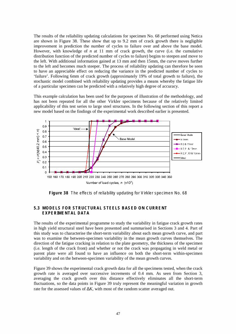
The results of the reliability updating calculations for specimen No. 68 performed using Netica are shown in Figure 38. These show that up to 9.2 mm of crack growth there is negligible improvement in prediction the number of cycles to failure over and above the base model. However, with knowledge of n at 11 mm of crack growth, the curve (i.e. the cumulative distribution function of the predicted number of cycles to failure) begins to steepen and move to the left. With additional information gained at 13 mm and then 15mm, the curve moves further to the left and becomes much steeper. The process of reliability updating can therefore be seen to have an appreciable effect on reducing the variance in the predicted number of cycles to ‘failure’. Following 6mm of crack growth (approximately 19% of total growth to failure), the stochastic model combined with reliability updating provides a means whereby the fatigue life of a particular specimen can be predicted with a relatively high degree of accuracy.

This example calculation has been used for the purposes of illustration of the methodology, and has not been repeated for all the other Virkler specimens because of the relatively limited applicability of this test series to large steel structures. In the following section of this report a new model based on the findings of the experimental work described earlier is presented.

Figure 38 The effects of reliability updating for Virkler specimen No. 68

5.3 MODELS FOR STRUCTURAL STEELS BASED ON CURRENT EXPERIMENTAL DATA

The results of the experimental programme to study the variability in fatigue crack growth rates in high yield structural steel have been presented and summarised in Sections 3 and 4. Part of this study was to characterise the short-term variability about each mean growth curve, and part was to examine the between-specimen variability in the mean growth curves themselves. The direction of the fatigue cracking in relation to the plate geometry, the thickness of the specimen (i.e. length of the crack front) and whether or not the crack was propagating in weld metal or parent plate were all found to have an influence on both the short-term within-specimen variability and on the between-specimen variability of the mean growth curves.

Figure 39 shows the experimental crack growth data for all the specimens tested, when the crack growth rate is averaged over successive increments of 0.4 mm. As seen from Section 3, averaging the crack growth over this distance effectively eliminates all the short-term fluctuations, so the data points in Figure 39 truly represent the meaningful variation in growth rate for the assessed values of ΔK, with most of the random scatter averaged out.

47

48

Figure 39 Pooled fatigue crack growth data – all specimens (0.4 mm increments) It has previously been noted that the assessed values of ΔK are likely to be reasonably close to the effective ΔK values experienced in service because the calculated values are based on the stress ranges Δσ which are likely to be known reasonably well if the amplitudes of the various components of the structural loading are themselves well defined. However, the presence of residual stresses in both the unwelded parent plate, resulting from steel manufacture, and in the welded regions, as a direct result of welding, will have effects on the stress ratio R and no attempt has been made to account for this in the present investigation. Indeed the stress ratio changes, even under constant amplitude loading, as the residual stresses become redistributed with crack growth. This is a difficult area which tends to be ignored in the fatigue assessment of full-scale structures. Figure 39 shows, however, that the effects described above tend to lower the fatigue crack growth rate below the typical design curves, resulting in slower fatigue crack growth than would be expected. This has a beneficial effect on some specimens but it cannot be relied upon. Finally, it may be concluded that the scatter of crack growth rates shown in Figure 39 is reasonably representative of what might be found in full-scale structures where it is almost impossible to know the distribution of residual stresses with any precision. In the remainder of this report somewhat different questions are addressed which relate to the process of reliability updating. What mathematical models of the fatigue behaviour of structural steels should be used in a reliability assessment, and how should the uncertainties in crack growth be modelled? These questions were examined in Section 5.2 for the fatigue of thin aluminium panels, but it is clear from the experimental data obtained for structural steels that more complex models are required to capture the various phenomena observed. In Section 3 it was demonstrated that fatigue crack growth rate profiles (i.e. plots of log(da/dN) versus log(ΔK)) for individual specimens can often be non-linear. This is a major departure from recommended fatigue crack growth laws in established codes of practice (e.g. BS7910). It was also observed that the variability in the fatigue crack growth rate about the each mean crack growth curve (when measured over consistent growth increments ∆a of 0.4 mm) was dependent on specimen thickness (i.e. crack front length), direction of crack propagation and on whether or not the fatigue crack was in the weld metal or parent plate. Some of these factors have been taken into account in developing a number of a priori models for reliability assessment.

5.3.1 Simple linear a Priori Crack Growth Model

The traditional approach to developing deterministic models for fatigue crack growth has been through the pooling of experimental data, as discussed in Section 1.1. However, the analysis of pooled data may be unreliable if the data set is inhomogeneous, since the overall variability in crack growth rate that is observed will then be made up of at least two components – (i) the random variations occurring within homogeneous sub-sets of material and (ii) systematic differences between the homogeneous sub-sets. As discussed above, it has been shown in the present work that detectable differences in fatigue crack growth rate occur as a result of differences in specimen geometry, thickness effects, direction of crack propagation, the presence of residual stresses, and probably for other reasons; and this raises the question of the extent to which these differences should be ignored in the development of fatigue models.

The pooling of inhomogeneous data sets always has the effect of increasing the sample variance, which in turn has the effect of elevating any design curve based on the concept of ‘mean plus two standard deviations’. This will result in a more conservative design than actually intended; but this is likely to be acceptable if it is not too uneconomic. However, for a reliability-based approach to design or assessment, reliance on pooled data may give rise to unrealistic results, especially if very low probabilities of failure are required for the structure. Therefore consideration should be given to developing quasi-homogeneous models for nominally similar specimens or situations. Nevertheless, where reliability updating is going to be used, it is possible to start with a generic a priori model and to use the additional data gained from the updating process to refine the reliability predictions.

The ‘physical’ or ‘mechanical’ model used for most fracture mechanics-based fatigue crack growth calculations is the linear Paris Law (Equation 1), or the bi-linear form of this adopted by BS7910. The simple linear model will initially be used in the following.

In Figure 34 it was shown, for the Virkler experiments, that a linear regression analysis of the ln(da/dN) vs ln(∆K) data for each specimen gave rise to a set of values of C and m which closely approximated a straight line when lnC was plotted against m, with the result that C could be approximated by

mln C = A + B (23) or

AC = (24)

Bm

A similar analysis has been undertaken on the experimental results from the current study of high strength steel for the 30 tests in which valid fatigue data were obtained. This is shown in Figure 40 in which log1 0 C is plotted against m. The four main classes of specimen are shown separately, and a linear regression has been performed for each.

It should be noted that the regression line for the welded beams should be ignored because of the very small sample size. For both beams, the data points lie within the main body of the other data, but the regression analysis gives unrealistic estimates of log1 0 C for large values of m. However, all the other data lie within a close band, with the lines for the non-welded beams and the non-welded CT specimens being more or less coincident. The line for the welded CT specimens lies below the other data, but it should be recalled that the large Hz and the smaller Vz specimens had significantly different fatigue growth characteristics (see Figure 31), and therefore form a non-homogeneous set. If the results for the Hz and Vz specimens are analysed as separate groups of data, the Vz specimens lie very close to the non-welded beam and CT data, and the Hz specimens lie on a separate line below the others (Figure 41).

49

Figure 40 Relationship between log10C and m for steel specimens (Note: the results for the welded beams should be ignored because of the small sample size)

Figure 41 Relationship between log10C and m for steel specimens (with Hz and Vz CT specimens considered separately)

Summarising these results, the values of the parameter C have been found to be:

1.570 ×10 −4

Non-welded Beams C = (25) (968.4 )m

2.304 ×10 −4

Non-welded CT (Hz and Vz) C = m

(26) (1019.2 )

2.075 ×10 −4

All non-welded specimens C = (27) (1003.9 )m

50

5.757 ×10 −4

Welded CT (Hz) C = (28) (1750.0 )m

1.530 ×10 −5

Welded CT (Vz) C = (29) (477.31 )m

2.558 ×10 −4

All welded CT (Hz and Vz) C = (30) (1485.3 )m

In Section 5.2.2 it was shown that the number of cycles to grow a fatigue crack to a critical size a can be computed by considering the summation of number of sets of cycles (ΔN) up to and including the critical size. When using the Paris Law as the crack growth model, this becomes

k k ∆a

N a ( ) =∑∆Ni =∑

m (6a) C(∆K )i =1 i=1 i

where Δa is an increment of growth and Δ is the number of cycles for the fatigue crack to Ni

grow the amount Δa in increment i.

Taking Δ → da and Δ → dN and using the same model as in Equation 17 (Section 5.2.3), with the independent error terms ε1 and ε2 derived from the relevant test data for the non-welded specimens taken as a single group, the number of cycles per growth increment of 0.4 mm is given by

a N

0.4 = ε ε 2 ) (31) dN da =0.4mm (−3.683 +m(log (∆K )−3.002) + +

10 10 1

with the parameters of m, ε and ε1 2 established from the fatigue test data as

2m ~ N (3.449, 0.5 ) 2ε1 ~ N (0, 0.0883 ) (32)

2ε2 ~ N (0, 0.1061 ) with ε1, ε2 and m being statistically independent normal distributed random variables. In calculating the numerical values of dN based on Equation 31, the values of ΔK have been calculated at the mid-point of each growth increment under consideration.

Figure 42 shows the linear a priori model and the ‘ideal’ model for Beam B1 based on crack increments of 0.4 mm. During testing, the crack grew from its original size of a0 = 5 mm to a =

17 mm (i.e. 30 × 0.4 mm increments) in 280,034 cycles of loading. The probability that the crack will grow from a0 to a in Nspec cycles of loading was computed from the event margin c

30 0.4

M = ∑

ε ε

− N (33) spec

i=1 -3.683 +m(log ( ΔK | ))-3.002 + + 2 i 10 10 a 1

51

c

Figure 42 a priori base model and ‘ideal’ model for beam specimen B1 for crack growth from 5 mm to 17 mm

Figure 42 shows that there is a large amount of uncertainty in the predicted number of loading cycles that will cause the crack to grow from a size of 5 mm to 17 mm (deemed the ‘failure’ event) when the predictions are based on the a priori model alone. One of the reasons for this is the large range of values for the C and m parameters for the non-welded specimens on which the model is based. In addition, the crack growth relationship for Beam B1 has been seen (Figure A3 in Appendix 1) to be far from linear. For these two reasons, the simple a priori model is not very satisfactory in its ability to predict fatigue crack growth, and will tend to overestimate the probability of fatigue failure for small numbers of loading cycles. For example, it can be seen from Figure 42 that the a priori model predicts the occurrence of ‘failure’ at about 1.7×105

cycles or less with a probability of approximately 1:100, which is well below the actual number of cycles to failure of about 280,000.

5.3.2 More advanced crack growth models

5.3.2.1 Generic Model Description

In order to try to improve the predictive capability of the a priori model, a generic third-order model based on 0.4 mm increments of crack growth has been investigated. This takes the form

0.4 dN =

10( (log10 ∆K| )3+c(log ∆K | )2 +d (log10 ∆K| )+e) (34)

b a 10 a a

where a is the current crack size and b, c, d and e are coefficients of a third-order polynomial. The main task in utilising such a model is the selection of appropriate values, or probability distributions, for the various coefficients. This is not easily achieved and therefore an alternative approach has been considered in what follows.

5.3.2.2 Special property of crack growth curves

Gurney (1978) has previously demonstrated that if Equation 24 is assumed to be exact, linear fatigue crack growth profiles with differing m parameters will all intersect at a unique point on the log da dN vs log ∆K plot. Figure 43 illustrates this phenomenon, plotting the data obtained by Virkler (1978), Gurney (1978) and the tests conducted as part of this research (see Appendices 1-4).

52

K

K

K

8

7

6

5

4

3

2

Virkler: = 344 Nmm3/2

Gurney: = 895 Nmm3/2

Pooled test data: = 1426 Nmm3/2

2.2 2.4 2.6 2.8 3 3.2 3.4

Log10 K )(Nmm3/2

Figure 43 Intersection of linear fatigue crack growth curves at unique points

These unique points of intersection of the crack growth curves have been referred to as the ‘Gurney point’ or ‘intersection point’ during the course of this work. If all the pairs of values (m, log10C) lie exactly on a straight line, as is almost the case for the individual types of specimen plotted in Figure 41, then the fatigue crack growth curves intersect at a single point

/when da dN is plotted against ΔK . Slight deviations of the data points from a straight line in Figure 41 clearly result in a fatigue crack growth curve which lies slightly above or below the ‘intersection point’, but very large deviations are required for the corresponding fatigue crack growth curve not to have at least approximately the characteristics shown in Figure 43. Examination of Figure 41 shows that for homogeneous sets of specimens (e.g. non-welded CT specimens) the data points (m, log10C) obey a closely linear relationship, and fatigue crack growth curves which roughly intersect are to be expected. This is generally the case for the current experimental data, but with some significant exceptions.

It is clear that the presence of an ‘intersection point’ provides a source of information by which more accurate predictions in the number of loading cycles for a crack to grow from ao to af can be made. To demonstrate this, Table 4 compares the computed number of cycles for a crack to grow from ao to af with the actual observed number of loading cycles for beams B1, B2, E1 and E2. The parameters of both the linear and third-order polynomial models (which in this case are taken to be deterministic) have been chosen so that the two theoretical fatigue crack growth curves pass through the ‘intersection point’, the co-ordinates of which correspond to the

/constant coefficients in Equation 25, and which are (968 Nmm-3 2; 1.570 × 10-4 mm/cycle). Numerical integration was then used to integrate the respective growth models over sequential increments of 0.4 mm to obtain the results in Table 4.

Table 4 Summary of actual loading cycles to failure and predicted number based on two models

Load ao af Actual Computed Computed Specimen Range mm mm Cycles Cycles Cycles 3rd

(kN) Linear Model order model B1 4.8-24 6.2 17.0 209,053 211,337 189,503 B2 4.8-24 6.0 21.0 296,622 278,306 266,648 E1 10.0-50 7.6 30.0 1,754,419 1,848,023 1,644,124 E2 4.8-24 6.3 19.8 433,626 655,018 417,894

53

The shape of the mean fatigue crack growth curve is the main factor in determining crack growth rates. As the crack is fully developed by the time it reaches size ao, the shape of the mean FCGR line can be determined by using the ‘intersection point’ and the average values of

dN da log and log ΔK from the first two recorded data points. For the linear model (which in this case is the simple Paris Law) the m parameter is computed from the slope of the log log da dN vs ΔK plot between the ‘intersection point’ and the average position of the first two data points corresponding to a growth increment of 0.4mm. The C parameter is computed through Equation 24. For the third-order model, only the specimen-specific mean fatigue crack growth rate is used.

It is demonstrated in Table 4 that by using the intersection point and crack growth data from early in the life of the specimen, reasonably accurate fatigue lives can be predicted using a linear model, provided the crack growth curves are indeed reasonably linear (e.g. specimens B1, B2 and E1). Comparable results are achieved using the third-order polynomial model passing through the ‘intersection point’. However for fatigue crack growth curves that are distinctly non-linear (e.g. E2) an accurate fatigue life prediction can only be made using a third order polynomial model passing through the ‘intersection point’.

5.3.2.3 Generic non-linear model

In Figure 44, the coordinates of the ‘intersection points’ determined from the data analysis in Section 5.3.1 have been plotted on the same graph as shown in Figure 3. The latter gives the mean curve presented by King (1998) together with lines drawn at two standard deviations above and below the mean and representing the scatter in historical fatigue crack growth data. It is of interest that in spite of the large amount of between-specimen variability in the fatigue crack growth curves in the present experimental work (see Figure 39) that these data have ‘intersection points’ determined from Equations 25- 30 which lie very close to the mean of the historical data.

Figure 44 Fatigue crack growth ‘intersection points’ for various classes of specimen

54

For non-welded specimens (both beams and CTs), the ‘intersection point’ for all the specimens /is at a value of ΔK of about 1,000 Nmm-3 2. The existence of such a point or region where the

crack growth curves tend to intersect implies that any specimen which is initially growing at a faster rate than the average at low values of ΔK (i.e. with small crack sizes, or low loads) will tend to grow less quickly (in relative terms) as the crack grows. Conversely, specimens in which the fatigue crack initially grows more slowly than the average will tend to increase their growth rate more quickly than the average, in order that the crack growth curve will pass through, or close to, the ‘intersection point’.

To develop a generic non-linear fatigue crack growth model similar to Equation 34, the ‘intersection point’ can be used in conjunction with a third-order polynomial fitted to pooled data. The specific crack growth profile for an observed crack following crack monitoring at an early stage in the life can therefore be determined by rotating this third-order polynomial about the assumed ‘intersection point’ such that the curve intersects the point corresponding to the observed value of dN da log and log ΔK . This is illustrated in Figure 45. Further details are given in Stanley (2005). However, it is clear that this model may be simplified by using only a linear form of crack growth model, if it is considered that in specific circumstances a non-linear model is not justified, but retaining the concept of the curve passing through the relevant intersection point.

i i l ial i i iFigure 45 Rotat on of th rd order po ynom about the ‘ ntersect on po nt’

5.3.3 Application of generic non-linear model

As an example of the use of the non-linear model, data has been taken from the early stages of the crack growth of Beam B1 and this has been used in conjunction with a third-order polynomial model developed from all the fatigue crack growth data for the non-welded beam specimens. The reliability calculations were performed using Netica and these are given in Figure 46. This shows the reliability predictions using the original linear a priori model from Figure 42, those based on the improved a priori third-order model without the inclusion of any specific information about Beam B1 itself, and finally the predictions updated with knowledge

da dN -3/2that the growth rate of beam B1 was observed as ≈ 7 ×10 −6 at ΔK ≈ 480 Nmm .

55

Figure 46 Reliability calculations for Beam B1

Figure 46 shows, for each of the three models, the computed probability that the number of 6loading cycles to ‘failure’ N will be less than n, over the range 0 ≤ n ≤ 10 , where ‘failure’ was

arbitrarily taken to be growth of the fatigue crack from an initial value of ao= 5.0 mm to a final value af = 17.0 mm. These can be compared with the ‘ideal’ model where there is no uncertainty in the fatigue crack growth process and which gives the actual number of cycles to cause ‘failure’ – in this case 280,034.

It can be seen from Figure 46 that incorporation of knowledge of the generic shape of the fatigue crack growth curve gives some improvement in reducing the variance of the predicted number of cycles of load to cause ‘failure’ (i.e. the curve becomes steeper in comparison with the linear a priori model). However, updating this prediction with information about the crack growth rate early in the specimen’s life has an even greater effect in reducing the uncertainty in the number of cycles to cause ‘failure’.

56

6 DISCUSSION AND CONCLUSIONS

At the start of this research it was known that structural steels, and indeed most other materials, exhibit considerable variability in fatigue crack growth behaviour. Lack of understanding about the source or sources of this variability makes the modelling of fatigue more difficult, which in turn affects the design and assessment processes, whether deterministic or probabilistic.

The original decision to study the fatigue properties of a single 50 mm thick steel plate was based on the assumption that the systematic differences would be small and that this would allow the proper characterisation of the random component of fatigue crack behaviour. However, the research has shown that even within a single as-rolled plate there are many factors which influence crack growth. Cutting and then welding the plate, not surprisingly, introduces further sources of variability.

As discussed in Section 1.4, fatigue tests were planned in order to answer a number of specific questions: • How does the rate of crack growth vary over short periods of time and over relatively small

amounts of crack extension? • What are the errors in assuming that fatigue cracking can be modelled by a linear or bi

linear law when considering a single crack growing under constant amplitude loading; and what is the corresponding model uncertainty?

• How does the crack growth rate vary between nominally identical specimens when loaded under nominally identical conditions?

• How does the thickness of the specimen and hence the length of the crack front influence the above?

• Is the rate of crack growth influenced by the direction of propagation in a plate? • How are all the above influenced when the crack grows through regions of welded material

where the crack front is likely to be sampling a range of micro-structures and where high magnitudes of residual stresses will be present?

The test programme has revealed new insights into most of these issues. It has been shown that for a single fatigue specimen (or structure), the variability in fatigue crack growth rate da/dN as a function of ΔK can be decomposed into local fluctuations about the mean rate at each value of ΔK, and changes in the mean rate with change in ΔK. In addition to this there are then random variations in the crack growth curves between nominally identical specimens, and systematic differences resulting from the effect of specimen thickness and direction of crack propagation, especially for welded specimens.

It has been seen that the short-term fluctuations in crack growth rate can be effectively eliminated by determining the average over crack extensions of about 0.5 mm. This source of variability has no influence on the prediction of fatigue life and will have an insignificant influence in any reliability assessment. However, the existence of these short-term fluctuations means that in the inspection and monitoring of existing structures, crack extensions of less than about 0.5 mm (assuming that these can be measured) would be of little value is assessing crack growth rates. The detailed findings from the experimental work are given in Section 4 and will not be summarised here.

In Section 5 the development of stochastic fatigue crack growth models has been investigated using data from the 1978 tests by Virkler and the data obtained from the current experimental work on structural steels. It has been demonstrated that the probabilistic models for the parameters in the fatigue crack growth relationships are, not surprisingly, dependent on the physical model selected to represent the fatigue crack growth process. For cases where a linear

57

crack growth relationship is a poor approximation to the real fatigue behaviour, the use of the Paris Law leads to additional uncertainty in computing the probability of fatigue failure and an increase in the variance of the fatigue life. However, it has been shown that even when a nonlinear crack growth model is used, the uncertainty in predicting fatigue life is still relatively large.

It has been demonstrated, however, that information gained from early stages in the fatigue life of a structure can be used to update the reliability predictions, and that this additional information can lead to a significant reduction in the variance of the predicted fatigue life. These conclusions derive from the finding that for a given geometry and material the fatigue crack growth curves show a tendency to intersect, or approximately intersect, at a particular value of range of stress intensity.

Finally, it must be emphasised that the research reported in this study has been based on fatigue tests carried out under constant amplitude loading and that further uncertainties in crack growth behaviour arise as soon as non-constant amplitude loading conditions are present. These can only increase the overall uncertainty in fatigue life prediction.

58

REFERENCES AND BIBLIOGRAPHY

ASTM (2001). Standard test methods for tension testing of metallic materials [metric]. ASTM.

Baker, M J and Stanley, I J (2002). An evaluation of reliability updating techniques for fatigue crack growth using experimental data. 1st ASRANet International Colloquium. Glasgow.

Ben-Gal I (2007). Bayesian Networks. In Ruggeri F, Faltin F, Kenett R. (Eds.), Encyclopedia of Statistics in Quality and Reliability, John Wiley & Sons.

British Standards Institution (1998). BS 6835-1: 1998, Method for the determination of the rate of fatigue growth in metallic materials: Fatigue growth rates of above 10-8 m per cycle. Milton Keynes: BSI.

British Standards Institution (1990). BS 4360: 1990, Specification for weldable structural steels. Milton Keynes: BSI.

British Standards Institution (2004). BS EN 10025: Part 2: 2004, Specification for non-alloy structural steels. Milton Keynes: BSI.

British Standards Institution (2005). BS 7910: 2005, Guide on methods for assessing the acceptability of flaws in metallic structures. Milton Keynes: BSI.

British Standards Institution (1991). BS PD6493: 1991 Guidance on methods for assessing the acceptability of flaws in welded structures. Milton Keynes: BSI.

Clark, WG Jr and Hudak, SJ Jr (1975). Variability in Fatigue Crack Growth Rate Testing, Journal of Testing and Evaluation, 3(6), pp. 454-476, 1975.

Ditlevsen, O and Olesen, O (1986). Statistical Analysis of the Virkler Data on Fatigue Crack Growth. Engineering Fracture Mechanics, 25(2), pp. 177-195, 1986.

Ditlevsen, O (1986). Random Fatigue Crack Growth – A First Passage Problem. Engineering Fracture Mechanics, 23(2), pp. 467-477, 1986.

Fett, T (1998). Stress intensity factors and weight functions for special crack problems. Institut für Materialforschung, FZKA 6025, Forschungszentrum Karlsruhe GmbH, Harlsruhe.

Gurney, TR (1978). An Analysis of Some Fatigue Crack Propagation Data for Steels Subjected to Pulsating Tension Loading, The Welding Institute, 59/1978/E.

Health and Safety Executive (2001). Probabilistic Methods: Uses and Abuses in Structural Integrity. Contract Research Report 398/2001, HSE.

Health and Safety Executive (2002). Review Of Probabilistic Inspection Analysis Methods, OTO 1999 061.

King, RN (1998). A Review of Fatigue Crack Growth Rates in Air and Seawater. Offshore Technology Report OTH 511. Norwich: HMSO.

King, RN, Stacey, A and Sharp, JV (1996). A Review of Fatigue Crack Growth Rates for

59

Offshore Steels in Air and Seawater Environments. Proceedings of the 15th OMAE, ASME, Vol. III , pp. 341-348.

Maddox, SJ (1974). Fatigue crack propagation data obtained from parent plate, weld metal and HAZ in structural steels. Welding Research International, 4 (1), pp36-60.

MTD (1992). Probability-based fatigue inspection planning. Report 92/100 London: Marine Technology Directorate Ltd.

Madsen, HO, Krenk, S and Lind, NC (1986). Methods of structural safety. Eaglewood Cliffs, NJ: Prentice Hall.

Matelect Ltd (2000a). Matelect ACPD Crack Growth Monitor – Type CGM-5R – Instruction Manual. London: Matelect Ltd.

Matelect Ltd (2000b). Matelect SM Modular Scanner System – Instruction Manual. London: Matelect Ltd.

Matelect Ltd (1993). Practical Aspects of the ACPD Technique, Users Manual. London: Matelect Ltd.

Melchers, RE (1999). Structural Reliability Analysis and Prediction (Civil Engineering). Chichester: John Wiley & Sons.

Miner, AM (1945). Cumulative Damage in Fatigue, Journal of Applied. Mechanics, pp. 151164.

Murakami, Y (1987). Stress Intensity Factors Handbook, Vol. 1 and Vol. 2. New York: Pergamon.

Nahar Hamid, Badrun (2006). A Methodology for the Reliability-Based Fracture Assessment of Structural Components Containing Cracks. PhD Thesis, University of Aberdeen, UK.

Norsys Software Corporation (1997). Netica Application User’s Guide. Norsys Software Corp., Vancouver, BC, Canada.

Ortiz, K and Kiremidjian, AS (1986). Time series analysis of fatigue crack growth rate data. Engineering Fracture Mechanics, 24(5), pp. 657-675.

Ostergaard, DF and Hillberry, BM (1983). Characterisation of the Variability in Fatigue Crack Propagation Data. Probabilistic Fracture Mechanics and Fatigue Methods; Applications for Structural Design and Maintenance, ASTM STP 798, American Society for Testing and Materials, pp. 97-115.

Ostergaard, DF, Thomas, JR and Hillberry, BM (1981). Effect of ∆a Increment on Calculating da/dN from a versus N Data. Fatigue Crack Growth Measurement and Data Analysis, ASTM STP 738, SJ Hudak Jr, and RJ Bucci, Eds, American Society for Testing and Materials, pp. 194204.

Paris, P and Erdogan, F (1963). A critical analysis of crack propagation laws. Journal of Basic Engineering, Trans ASME, 85, pp.528-534.

Paris, PC, Gomez, MP and Anderson, WP (1961). A rational analytic theory of fatigue. The Trend in Engineering, 13, pp. 9-14.

60

Parker, AP (1982). Stress Intensity Factors, Crack Profiles, and Fatigue Crack Growth Rates in Residual Stress Fields, in Residual Stress Effects in Fatigue, ASTM STP 776, ASTM, pp. 1331.

Pook, LP (1975). Basic Statistics of Fatigue Crack Growth, NEL Report No. 595, National Engineering Laboratory.

Proppe, C and Schuëller, M (2000). “Statistical Processing of Fatigue Crack Growth Data”, 8th ASCE Speciality Conference on Probabilistic Mechanics and Structural Reliability, PMC2000, ASCE.

Righiniotis, TD and Chryssanthopoulos, MK (2003). Probabilistic fatigue analysis under constant amplitude loading. Journal of Constructional Steel Research, 59 (5), pp. 867-886.

Rooke DP and Cartwright DJ (1976). Compendium of stress intensity factors. Her Majesty’s Stationary Office, London.

Schijve, J (1988). Fatigue Predictions and Scatter. Fatigue and Fracture of Engineering Materials and Structures, 17(4), pp. 5-34, 1988.

Smith, RA (1984). Thirty Years of Fatigue Crack Growth – A Historical Review in Fatigue Crack Growth 30 Years of Progress. Proceedings of a Conference on Fatigue Crack Growth, Cambridge, UK.

Stacey A, Birkinshaw, M and Sharp JV (2001). Life Cycle Integrity of North Sea Installations. Proc 11th International Offshore and Polar Engineering Conference, Stavanger, ISOPE.

Stanley, IG (2005). Improved Methods for Reliability-Based Structural Integrity Assessment of Steel Jacket Structures. PhD Thesis, University of Aberdeen, UK.

Tanaka, S, Ichikawa, M and Akita, S (1981). Variability of m and C in the fatigue crack propagation law da/dN=C(∆K)m . International Journal of Fracture, 17, R121-124..

Thoft-Christensen, P and Baker, MJ (1982). Structural Reliability Theory and Its Applications. Berlin: Springer-Verlag.

Tong, J (2002). T-stress and its implications for crack growth. Engineering Fracture Mechanics, 69, pp. 1325-1337.

Tvedt, L (2006). Proban – probabilistic analysis. Structural Safety, 28, pp. 150-163.

Virkler, DA, Hillberry, BM, and Goel, PK (1978). The Statistical Nature of Fatigue Crack Propagation, AFFDL-TR-78-43, Air Force Flight Dynamics Laboratory.

Virkler, DA, Hillberry, BM, Goel, PK (1979). The Statistical Nature of Fatigue Crack Propagation. Trans ASME, Journal of Engineering Materials and Technology, 101, pp.148-153.

ZENCRACK (2004). Automatic 3-D Fracture Mechanics Mesh Generation Software, Version 7.3. 2004. Zentech Inc, USA.

61

APPENDIX 1 EXPERIMENTAL FATIGUE DATA FOR NON-WELDED

BEAM SPECIMENS

Page

Figure A1 Crack growth rates for beam E1 (0.4 and 0.8 mm increments) 64

Figure A2 Crack growth rates for beam E2 (0.4 and 0.8 mm increments) 64

Figure A3 Crack growth rates for beam B1 (0.4 and 0.8 mm increments) 65

Figure A4 Crack growth rates for beam B2 (0.4 and 0.8 mm increments) 65

Table A1 Details of non-welded beam tests

Serial No. Span Depth Thickness Pmax Pmin Figs.

S (mm) W (mm) B (mm) kN kN

E1 500 100

E2 500 50

B1 500 50

B2 500 50

50 50.0 10.0 A1

50 24.0 4.8 A2

50 24.0 4.8 A3

50 24.0 4.8 A4

NOTE ON CURVE FITTING PROCEDURE

Appendices 1-4 have been included in this report to enable the reader to see directly the variation in fatigue crack growth rates that were exhibited by each specimen. In most cases it has been possible to fit a smooth curve to represent the change in mean crack growth rate with crack extension, and these curves have been used in the body of the report to make comparisons between different specimens. In some cases however, because of the irregularity of the growth (e.g. Figure A32) no curve fitting has been attempted.

A pragmatic approach has been used to the fitting of the mean curves, with power curves and third and fourth order polynomials being used as appropriate, the aim being to get a single curve for each test specimen that represents the mean growth rate as well as possible over the complete range of the experimental data.

63

da/d

N (

mm

/cyc

le)

1.E-03

1.E-04

1.E-05

1.E-06 100 1,000 10,000

/2)ΔK (Nmm-3

Figure A1 Crack growth rates for beam E1 (0.4 and 0.8 mm increments)

//

l

1.E-06

1.E-05

1.E-04

1.E-03

dadN

(m

mcy

ce)

100 1,000 10,000 /2)ΔK (Nmm-3

Figure A2 Crack growth rates for beam E2

(0.4 and 0.8 mm increments)

64

100

100

//

l

1.E-06

1.E-05

1.E-04

1.E-03 da

dN (

mm

cyc

e)

1,000 10,000

/2)ΔK (Nmm-3

Figure A3 Crack growth rates for beam B1


//

l

1.E-06

1.E-05

1.E-04

1.E-03

dadn

(m

mcy

ce)

1,000 10,000

/2)ΔK (Nmm-3

Figure A4 Crack growth rates for beam B2


65

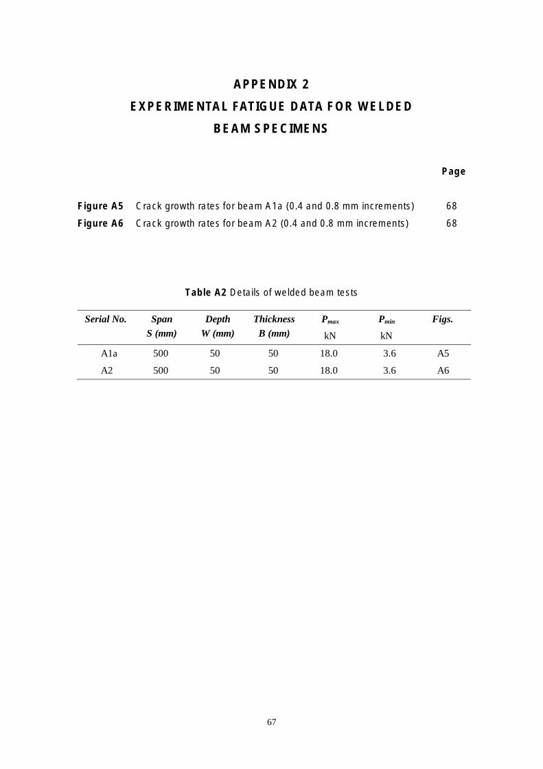
APPENDIX 2

EXPERIMENTAL FATIGUE DATA FOR WELDED

BEAM SPECIMENS

Page

Figure A5 Crack growth rates for beam A1a (0.4 and 0.8 mm increments) 68

Figure A6 Crack growth rates for beam A2 (0.4 and 0.8 mm increments) 68

Table A2 Details of welded beam tests

Serial No. Span Depth Thickness Pmax Pmin Figs. S (mm) W (mm) B (mm) kN kN

A1a 500 50 50 18.0 3.6 A5

A2 500 50 50 18.0 3.6 A6

67

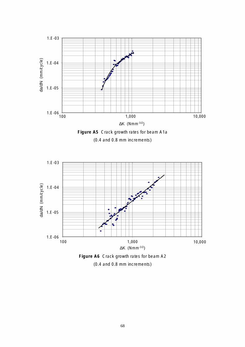
100

100

//

l

1.E-06

1.E-05

1.E-04

1.E-03 da

dN (

mm

cyc

e)

1,000 10,000 /2)ΔK (Nmm-3

Figure A5 Crack growth rates for beam A1a


//

l

1.E-06

1.E-05

1.E-04

1.E-03

dadN

(m

mcy

ce)

1,000 10,000 /2)ΔK (Nmm-3

Figure A6 Crack growth rates for beam A2


68

APPENDIX 3

EXPERIMENTAL FATIGUE DATA FOR NON-WELDED

CT SPECIMENS

Page

Figure A7 Crack growth rates for CT specimen Hz D1 (0.05 mm incs) 71

Figure A8 Crack growth rates for CT specimen Hz D1 (0.4 and 0.8 mm incs) 71

Figure A9 Crack growth rates for CT specimen Hz D2-1 (0.05 mm incs) 72

Figure A10 Crack growth rates for CT specimen Hz D2-1 (0.4 and 0.8 mm incs) 72









Figure A19 Crack growth rates for CT specimen Vz E1 (0.05 mm incs) 77

Figure A20 Crack growth rates for CT specimen Vz E1 (0.4 and 0.8 mm incs) 77

Figure A21 Crack growth rates for CT specimen Vz E2-2 (0.05 mm incs) 78

Figure A22 Crack growth rates for CT specimen Vz E2-2 (0.4 and 0.8 mm incs) 78







69

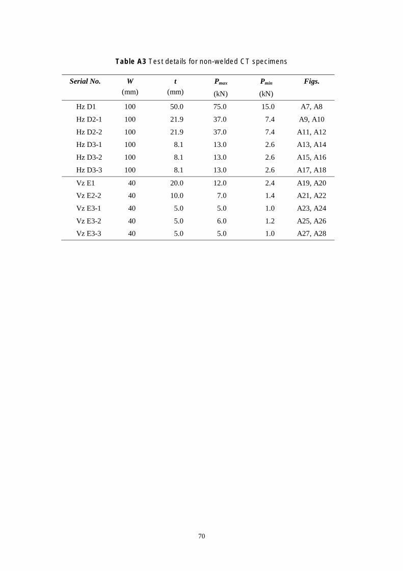
Table A3 Test details for non-welded CT specimens

Serial No. W t Pmax Pmin Figs. (mm) (mm) (kN) (kN)

Hz D1 100 50.0 75.0 15.0 A7, A8

Hz D2-1 100 21.9 37.0 7.4 A9, A10

Hz D2-2 100 21.9 37.0 7.4 A11, A12

Hz D3-1 100 8.1 13.0 2.6 A13, A14

Hz D3-2 100 8.1 13.0 2.6 A15, A16

Hz D3-3 100 8.1 13.0 2.6 A17, A18

Vz E1 40 20.0 12.0 2.4 A19, A20

Vz E2-2 40 10.0 7.0 1.4 A21, A22

Vz E3-1 40 5.0 5.0 1.0 A23, A24

Vz E3-2 40 5.0 6.0 1.2 A25, A26

Vz E3-3 40 5.0 5.0 1.0 A27, A28

70

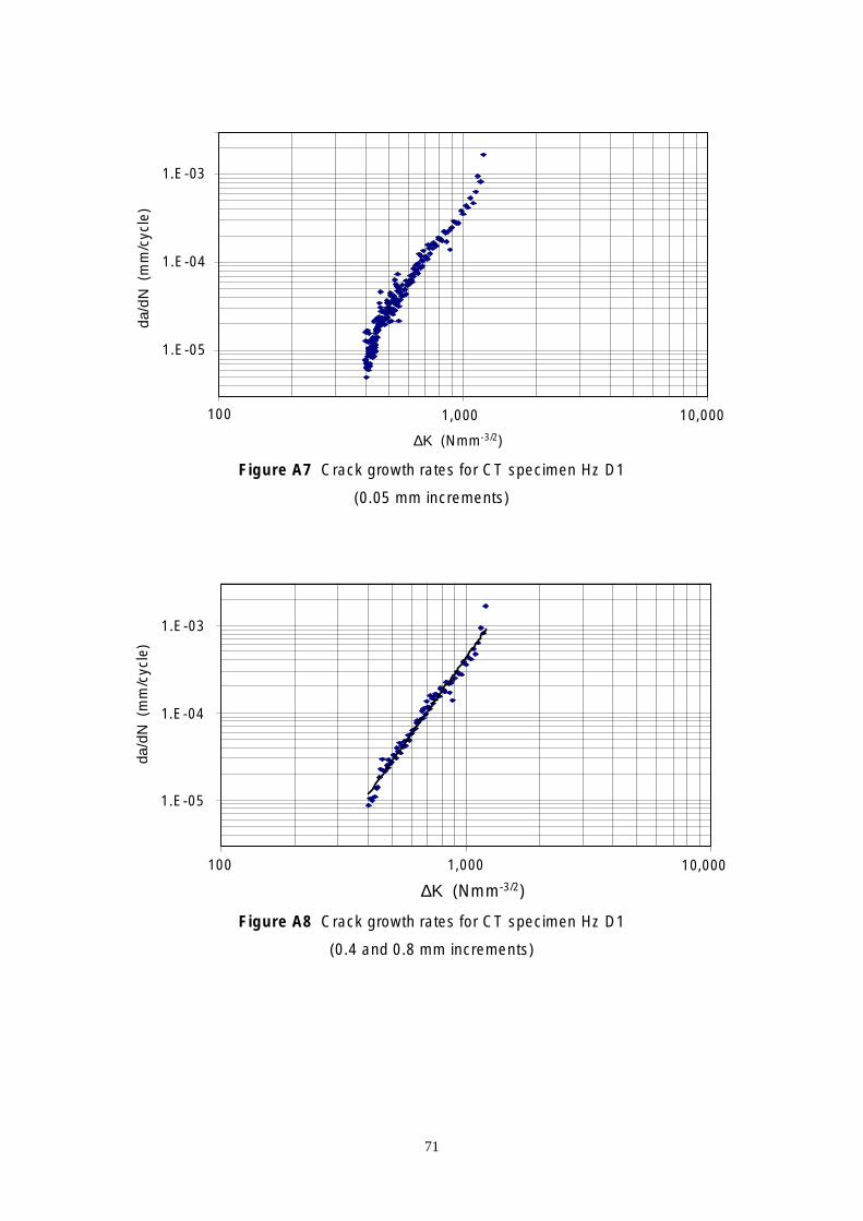
100

100

//

l

1.E-05

1.E-04

1.E-03

dadN

(m

mcy

ce)

1,000 10,000 /2)ΔK (Nmm-3

Figure A7 Crack growth rates for CT specimen Hz D1

(0.05 mm increments)

//

l

1.E-05

1.E-04

1.E-03

dadN

(m

mcy

ce)

1,000 10,000 /2)ΔK (Nmm-3

Figure A8 Crack growth rates for CT specimen Hz D1


71

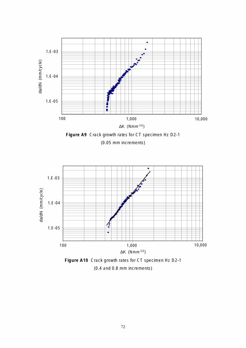
100

100

//

l

1.E-05

1.E-04

1.E-03

dadN

(m

mcy

ce)

1,000 10,000 /2)ΔK (Nmm-3

Figure A9 Crack growth rates for CT specimen Hz D2-1


//

l

1.E-05

1.E-04

1.E-03

dadN

(m

mcy

ce)

1,000 10,000 /2)ΔK (Nmm-3



72

100

100

//

l

1.E-05

1.E-04

1.E-03

dadN

(m

mcy

ce)

1,000 10,000

/2)ΔK (Nmm-3



//

l

1.E-05

1.E-04

1.E-03

dadN

(m

mcy

ce)

1,000 10,000

/2)ΔK (Nmm-3



73

74

1.E-06

1.E-05

1.E-04

1.E-03

100 1,000 10,000

ΔK (Nmm-3/2)

da/d

N (

mm

/cyc

le)



1.E-05

1.E-04

1.E-03

100 1,000 10,000

ΔK (Nmm-3/2)

da/d

N (

mm

/cyc

le)



100

100

//

l

1.E-06

1.E-05

1.E-04

1.E-03 da

dN (

mm

cyc

e)

1,000 10,000

/2)ΔK (Nmm-3



//

l

1.E-05

1.E-04

1.E-03

dadN

(m

mcy

ce)

1,000 10,000

/2)ΔK (Nmm-3



75

76

1.E-06

1.E-05

1.E-04

1.E-03

100 1,000 10,000

ΔK (Nmm-3/2)

da/d

N (

mm

/cyc

le)



1.E-05

1.E-04

1.E-03

100 10,000ΔK (Nmm-3/2)

da/d

N (

mm

/cyc

le)

1,000



100

100

//

l

1.E-06

1.E-05

1.E-04

1.E-03 da

dN (

mm

cyc

e)

1,000 10,000 /2)ΔK (Nmm-3

Figure A19 Crack growth rates for CT specimen Vz E1


//

l

1.E-06

1.E-05

1.E-04

1.E-03

dadN

(m

mcy

ce)

1,000 10,000 /2)ΔK (Nmm-3

Figure A20 Crack growth rates for CT specimen Vz E1


77

//

l

1.E-06

1.E-05

1.E-04

1.E-03

dadN

(m

mcy

ce)

100 1,000 10,000 /2)ΔK (Nmm-3

Figure A21 Crack growth rates for CT specimen Vz E2-2


da/d

N (

mm

/cyc

le)

1.E-03

1.E-04

1.E-05

1.E-06 100 1,000 10,000

/2)ΔK (Nmm-3



78

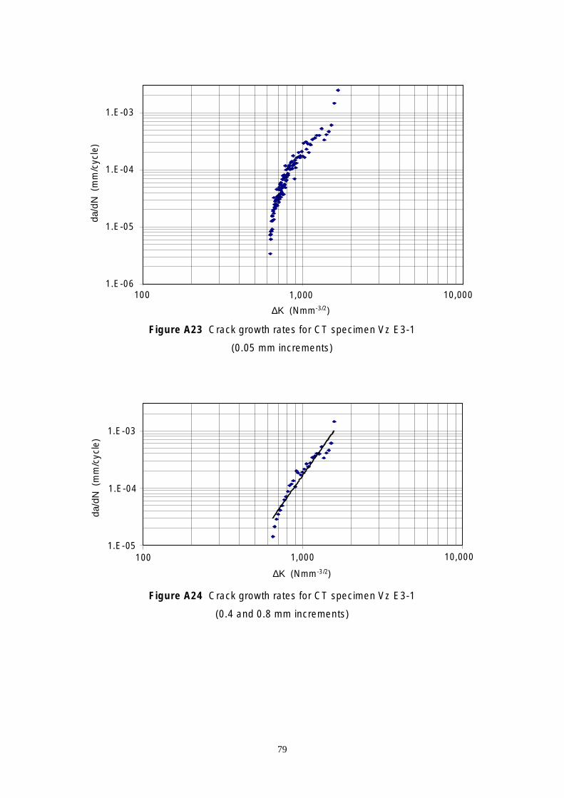
100

100

//

l

1.E-06

1.E-05

1.E-04

1.E-03

dadN

(m

mcy

ce)

1,000 10,000 /2)ΔK (Nmm-3



//

l

1.E-05

1.E-04

1.E-03

dadN

(m

mcy

ce)

1,000 10,000 /2)ΔK (Nmm-3



79

da/d

N (

mm

/cyc

le)

1.E-03

1.E-04

1.E-05

1.E-06 100 1,000 10,000

/2)ΔK (Nmm-3



//

l

1.E-05

1.E-04

1.E-03

dadN

(m

mcy

ce)

100 1,000 10,000 /2)ΔK (Nmm-3



80

//

l

1.E-05

1.E-04

1.E-03

dadN

(m

mcy

ce)

100 1,000 10,000

/2)ΔK (Nmm-3



da/d

N (

mm

/cyc

le)

1.E-03

1.E-04

1.E-05 100 1,000 10,000

/2)ΔK (Nmm-3



81

APPENDIX 4

EXPERIMENTAL FATIGUE DATA FOR WELDED CT SPECIMENS

Page

Figure A29 Crack growth rates for CT specimen Hz C1 (0.05 mm incs) 85

Figure A30 Crack growth rates for CT specimen Hz C1 (0.4 and 0.8 mm incs) 85

Figure A31 Crack growth rates for CT specimen Hz C2-1 (0.05 mm incs) 86

Figure A32 Crack growth rates for CT specimen Hz C2-1 (0.4 and 0.8 mm incs) 86


Figure A34 Crack growth rates for CT specimen Hz C2-2 (0.4 and 0.8mm incs) 87









Figure A43 Crack growth rates for CT specimen Vz C4 (0.05 mm incs) 92

Figure A44 Crack growth rates for CT specimen Vz C4 (0.4 and 0.8 mm incs) 92











83

Table A4 Test details for welded CT specimens

Serial No. W t Pmax Pmin Figs. (mm) (mm) (kN) (kN)

Hz C1 100 50.0 126.0 25.2 A29, A30

Hz C2-1 100 21.9 67.0 13.4 A31, A32

Hz C2-2 100 21.9 65.0 13.0 A33, A34

Hz C3-1 100 8.1 30.0 6.0 A35, A36

Hz C3-2 100 8.1 24.0 4.8 A37, A38

Hz C3-3 100 8.1 24.0 4.8 A39, A40

Hz C3-4 100 8.1 28.0 5.6 A41, A42

Vz C4 40 20.0 12.0 2.4 A43, A44

Vz C5 40 10.0 6.0 1.2 A45, A46

Vz C6 40 10.0 6.0 1.2 A47, A48

Vz C7 40 5.0 3.0 0.6 A49, A50

Vz C9 40 5.0 7.0 1.4 A51, A52

Vz C10 40 5.0 7.0 1.4 A53, A54

84

//

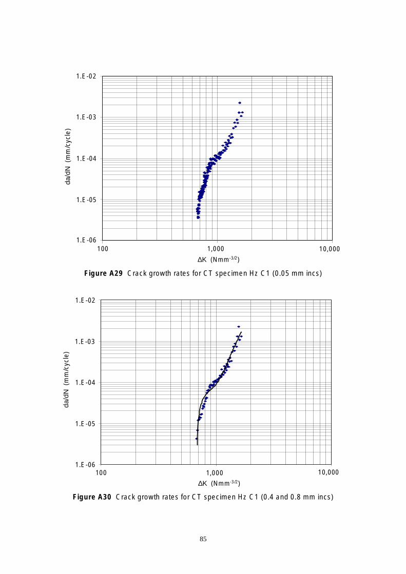
l

1.E-06

1.E-05

1.E-04

1.E-03

1.E-02 da

dN (

mm

cyc

e)

100 1,000 10,000 /2)ΔK (Nmm-3

Figure A29 Crack growth rates for CT specimen Hz C1 (0.05 mm incs)

//

l

1.E-06

1.E-05

1.E-04

1.E-03

1.E-02

dadN

(m

mcy

ce)

100 1,000 10,000 /2)ΔK (Nmm-3

Figure A30 Crack growth rates for CT specimen Hz C1 (0.4 and 0.8 mm incs)

85

//

l

1.E-06

1.E-05

1.E-04

1.E-03

1.E-02 da

dN (

mm

cyc

e)

100 1,000 10,000 /2)ΔK (Nmm-3

Figure A31 Crack growth rates for CT specimen Hz C2-1 (0.05 mm incs)

da/d

N (

mm

/cyc

le)

1.E-02

1.E-03

1.E-04

1.E-05

1.E-06 100 1,000 10,000

/2)ΔK (Nmm-3

Figure A32 Crack growth rates for CT specimen Hz C2-1 (0.4 and 0.8 mm incs)

86

//

l

1.E-06

1.E-05

1.E-04

1.E-03

1.E-02 da

dN (

mm

cyc

e)

100 1,000 10,000 /2)ΔK (Nmm-3


//

l

1.E-06

1.E-05

1.E-04

1.E-03

1.E-02

dadN

(m

mcy

ce)

100 1,000 10,000 /2)ΔK (Nmm-3

Figure A34 Crack growth rates for CT specimen Hz C2-2 (0.4 and 0.8mm incs)

87

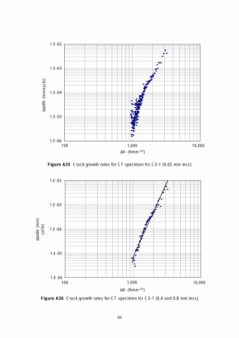
/m

/l

1.E-06

1.E-05

1.E-04

1.E-03

1.E-02 da

dN (

mcy

ce)

100 1,000 10,000 /2)ΔK (Nmm-3


da/d

N (

mm

/ cy

cle)

1.E-02

1.E-03

1.E-04

1.E-05

1.E-06 100 1,000 10,000

/2)ΔK (Nmm-3


88

//

l

1.E-06

1.E-05

1.E-04

1.E-03

1.E-02 da

dN

(mm

cyc

e)

100 1,000 10,000 /2)ΔK (Nmm-3

Figure A37 Crack growth rates for CT specimen Hz C3-2 (0.05 mm increments)

da/d

N (

mm

/cyc

le)

1.E-02

1.E-03

1.E-04

1.E-05

1.E-06 100 1,000 10,000

/2)ΔK (Nmm-3


89

//

l

1.E-06

1.E-05

1.E-04

1.E-03

1.E-02 da

dN

(mm

cyc

e)

100 1,000 10,000 /2)ΔK (Nmm-3


da/d

N

(mm

/cyc

le)

1.E-02

1.E-03

1.E-04

1.E-05

1.E-06 100 1,000 10,000

/2)ΔK (Nmm-3


90

//

l

1.E-06

1.E-05

1.E-04

1.E-03

1.E-02 da

dN (

mm

cyc

e)

100 1,000 10,000 /2)ΔK (Nmm-3


da/d

N (

mm

/cyc

le)

1.E-02

1.E-03

1.E-04

1.E-05

1.E-06 100 1,000 10,000

/2)ΔK (Nmm-3


91

iFigure A43 Crack growth rates for CT specimen Vz C4 (0.05 mm ncs)

K )(Nmm 3/2

Figure A44 Crack growth rates for CT specimen Vz C4 (0.4 and 0.8 mm

da/dN (m

m/cycle)

1.E03

1.E04

1.E05

1.E06 100 1,000 10,000

incs)

92

1.E06

1.E05

1.E04

1.E03

100 1,000 10,000

Figure A45 Crack growth rates for CT specimen Vz C5 (0.05 mm incs)

iFigure A46 Crack growth rates for CT specimen Vz C5 (0.4 and 0.8 mm ncs)

93

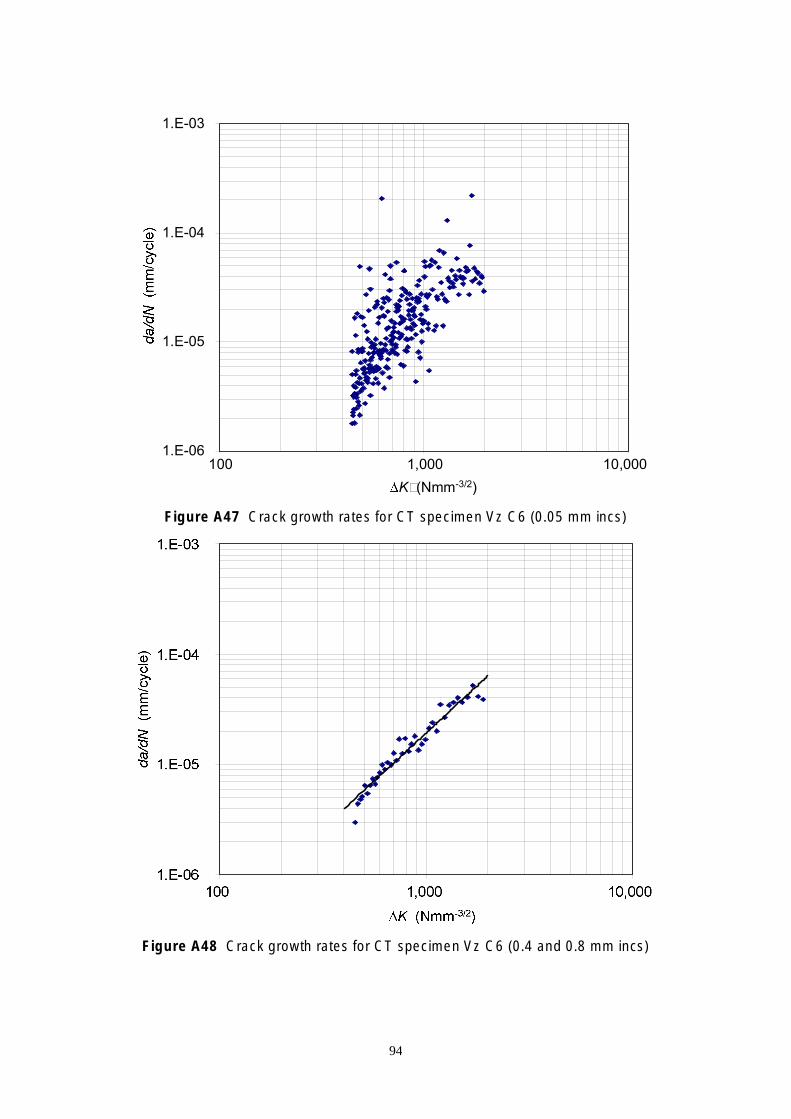
100 1.E06

1.E05

1.E04

1.E03

1,000 10,000

K )

i

i

(Nmm3/2

Figure A47 Crack growth rates for CT specimen Vz C6 (0.05 mm ncs)

Figure A48 Crack growth rates for CT specimen Vz C6 (0.4 and 0.8 mm ncs)

94

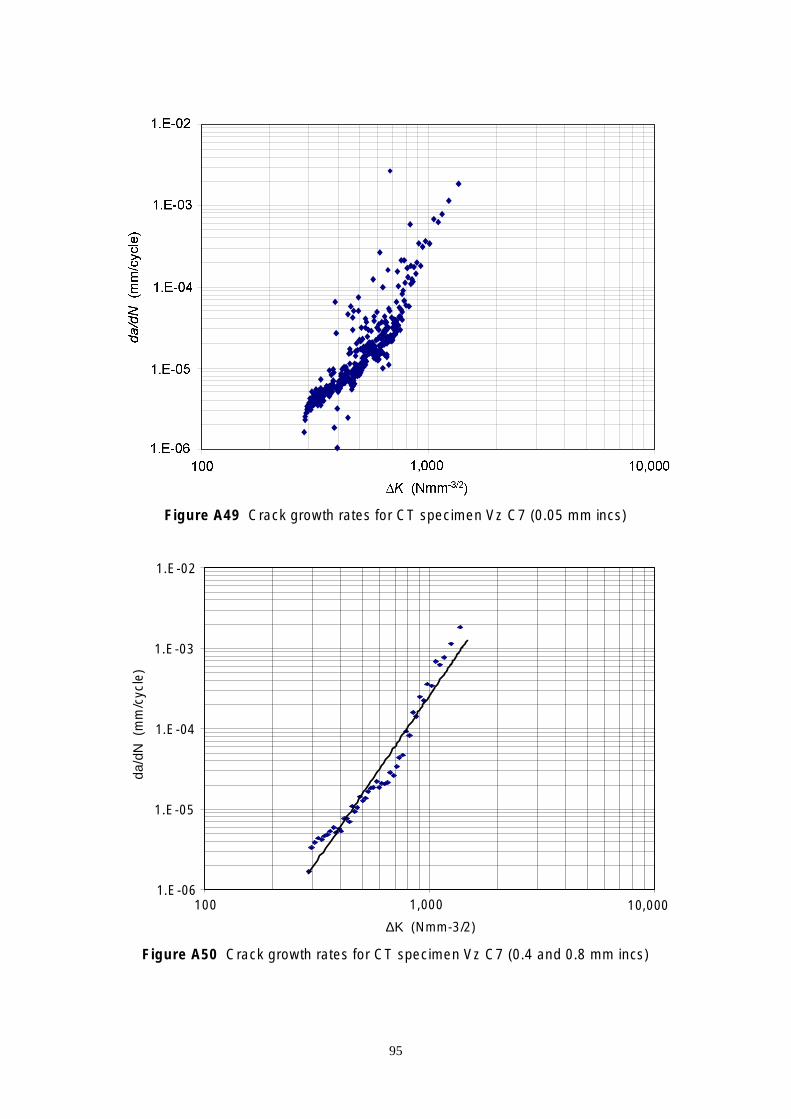
iFigure A49 Crack growth rates for CT specimen Vz C7 (0.05 mm ncs)

da/d

N (

mm

/cyc

le)

1.E-02

1.E-03

1.E-04

1.E-05

1.E-06 100 1,000 10,000

ΔK (Nmm-3/2)

Figure A50 Crack growth rates for CT specimen Vz C7 (0.4 and 0.8 mm incs)

95

//

l

1.E-06

1.E-05

1.E-04

1.E-03

1.E-02 da

dn (

mm

cyc

e)

100 1,000 10,000 /2)ΔK (Nmm-3

Figure A51 Crack growth rates for CT specimen Vz C9 (0.05 mm incs)

//

l

1.E-06

1.E-05

1.E-04

1.E-03

1.E-02

dadN

(m

mcy

ce)

100 1,000 10,000 /2)ΔK (Nmm-3

Figure A52 Crack growth rates for CT specimen Vz C9 (0.4 and 0.8 mm incs)

96

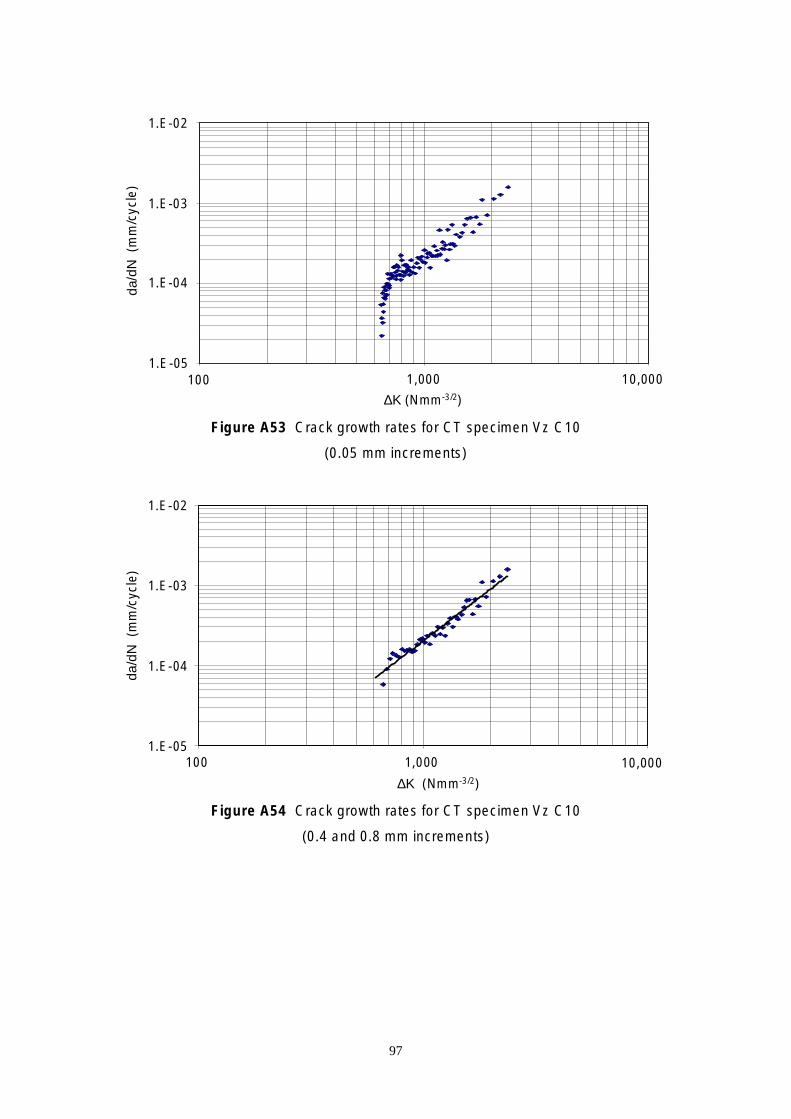
100

100

//

l

1.E-05

1.E-04

1.E-03

1.E-02 da

dN (

mm

cyc

e)

1,000 10,000 /2)ΔK (Nmm-3

Figure A53 Crack growth rates for CT specimen Vz C10


//

l

1.E-05

1.E-04

1.E-03

1.E-02

dadN

(m

mcy

ce)

1,000 10,000 /2)ΔK (Nmm-3

Figure A54 Crack growth rates for CT specimen Vz C10


97

Published by the Health and Safety Executive 07/08



The prediction of the fatigue life of steel structures can be carried out in a number of different ways. A common method at the design stage is to use the so-called S-N approach using design data from a standard such as BS 7910. However, for existing structures containing defects of a known or postulated size, a fatigue life assessment is generally carried out using fracture mechanics. In keeping with normal engineering practice, it is usual to calculate conservative (safe) estimates of fatigue life, although occasionally best estimates may also be of interest. For more advanced structural assessments, reliability-based methods can be used to calculate the remaining life corresponding to a number of different probabilities of failure (eg 10-4, 10-6). The motivation for the research reported here was the need to improve the current methods of reliability assessment for structures, and in particular steel offshore structures approaching the end of their design lives. As part of this research, work was carried out to investigate the variability in the fatigue crack growth of steels and the way in which the corresponding uncertainties could best be incorporated into the assessment process. This included the fatigue testing of specimens of BS 4360: 1990 Grade 50DD steel with the explicit aim of studying the variability in crack growth under different conditions. The results of these tests are presented in this research report. The relatively large uncertainties associated with fatigue crack growth behaviour, even within relatively homogenous sets of specimens, means that the variance in the predicted fatigue life is relatively large. It has been shown, however, that the use of fatigue crack growth rate data from relatively early in the life of a particular structure can significantly reduce this uncertainty and improve the reliability predictions through the process of reliability updating.

This report and the work it describes were funded by the Health and Safety Executive (HSE). Its contents, including any opinions and/or conclusions expressed, are those of the authors alone and do not necessarily reflect HSE policy.

RR643

www.hse.gov.uk

rr643 assessing and modelling the uncertainty in fatigue crack

Documents