rpsea review meeting april 6-7, 2010, golden, co 1 optimizing in fill well drilling - wamsutter...

RPSEA Review Meeting

April 6-7, 2010, Golden, CO1

Optimizing In Fill Well Drilling - Wamsutter Field

Mohan Kelkar

The University of Tulsa

Akhil Datta-Gupta

Texas A & M University



Outline

• Background• Objectives• Project Management• Project Deliverables• Progress to Date• Summary



Wamsutter Field



Wamsutter Field

•Over 2,000 square miles•Two main units – Lewis and

Almond• Tight gas reservoir, k < 0.1 md•Currently developed on 80 acre

spacing



Wamsutter FieldStatic Continuity



Static vs. Dynamic Continuity

• Static continuity appears to be strong indicating a significant and efficient drainage using 160 acre spacing

• Small scale heterogeneities in the reservoir indicate significant dynamic discontinuities

• The presence of small scale heterogeneities is verified by performance of 80 acre spacing wells

• Average performance of 80 acre spacing wells is 50 to 70 % of the performance of 160 acre spacing wells



Objectives

• Determine and quantify the importance of small scale heterogeneities on the performance of wells

• Quantify the potential recovery from in fill wells using production data analysis as well as simulation

• Identify sweet spots for possible locations for 40 acre spacing wells



Project Management

• Principal Investigator – The University of Tulsa

• SubcontractorsDevon EnergyTexas A & M University

• Based on the results of the study, Devon is planning to drill seven new wells in the field



Project Deliverables

• Methodology to determine the incremental vs. acceleration gas production from in fill wells

• Methodology to account for and, preservation of, sand connectivity in coarse scale models

• Procedures for high and low grading areas for in fill well potential



Progress to DateArea of Concentration



Data Collected

• Area of interest is 3x3 sections in 16N 93 W township with one additional section on all sides which covers 5 x5 sections (total of 25 sections)

• A total of 83 wells are drilled in the area• Log data as well as production data are

available from most of the wells



Production Data Analysis

University of Tulsa



Introduction

• Homogeneous and heterogeneous reservoirs will exhibit different behavior when in fill wells are drilled: Initial production rates will indicate access

to new reservesDifference in decline rates from the

surrounding wells will indicate communication



Homogeneous Reservoir

×: Original well○: Infill wells

0 5 10 15 20 25 30 35 400

1

2

3

4

5

6

7

Original well

Infill well

Drill new wells



Heterogeneous Reservoir

×: Original well○: Infill wells

0 5 10 15 20 25 30 35 400

1

2

3

4

5

6

7

Original well

Infill well

Drill new wells



Objectives

• Develop a methodology to predict the gas which is “stolen” by new wells.

• Using the existing production data, determine the in fill well EUR

• Determine the contribution of acceleration and incremental potential.



Approach

• Determine an appropriate time function such that cumulative production is linearly related.

• Divide the data into chronological groups so that average behavior can be predicted.

• Plot cum production vs. time function and examine inflection in the graph as successive groups of wells are drilled.

• Compare EUR calculated from this method with the EUR reported by companies.



Southwest Energy



Type Curve ExtrapolationSouthwest Energy



Chesapeake Energy



Type Curve ExtrapolationChesapeake Energy



Approach

• Determine a function of time such that cumulative production is directly related.






Field Data

183050 183550 184050 184550 185050 185550 1860501434000

1434500

1435000

1435500

1436000

1436500

1437000

1437500

1438000

1438500

123456

7 8 9 10 11 12

131415161718

19 20 21 22 23 24

30 29 28 27 26 25

31 32 33 34 35 36



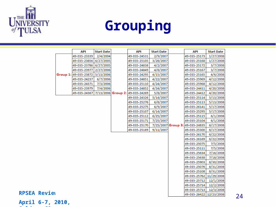
Grouping



Approach







Example



Approach



• Plot cum production vs. time function and examine inflection in the graph as successive group of wells are drilled.




EUR Comparison

0 1 2 3 4 5 6 70

1

2

3

4

5

6

7

EUR(TU), Bscf

EU

R(O

per

ato

r),

Bsc

f



Group EUR Comparison

EUR(ours) EUR(Operator)

1st group 3.31 3.32

2nd group 3.01 3.07

3rd group 2.32 2.34



Approach

• For every “child” well, calculate average Incremental and Acceleration components.

• Plot Acceleration percentage, Incremental percentage and total EUR as a function of spacing.

• Recommend potential sections where in fill well potential is the greatest.



Calculation

• Acceleration vs. IncrementalTotal EUR for 2nd group per well = 3.57 BCFAcceleration EUR for 2nd group per well

= Decreased EUR = 0.24 BCF Incremental EUR for 2nd group per well

= Total EUR - Acceleration EUR

= 3.57 - 0.24 = 3.33 BCF



Approach

• For every “child” well, calculate average Incremental and Acceleration component.





Wamsutter FieldMultiple Section Analysis

225352.784699999 226902.709091999 228452.633483999 230002.557875999 231552.482267999 233102.40665999974851.19

76511.995457

78172.800914

79833.606371

81494.411828

83155.217285

1 2 3 4 5

6 7 8 9 10

11 12 13 14 15

16 17 18 19 20

21 22 23 24 25



ACC vs. INCE-W direction

120 175 384 6400.000

0.500

1.000

1.500

2.000

2.500

3.000

3.500

4.000

4.500

5.000

0%

10%

20%

30%

40%

50%

60%

70%

80%

90%

100%

EW-7,8,9ACC+INC

ACC%

INC%

Spacing, acre

AC

C+

INC

,bs

cf

AC

C&

INC

%



ACC vs. INCN-S direction

91 128 320 4800.000

1.000

2.000

3.000

4.000

5.000

6.000

0%

10%

20%

30%

40%

50%

60%

70%

80%

90%

100%

NS-9,14,19ACC+INC

ACC%

INC%

Spacing, acre

AC

C+

INC

,bs

cf

AC

C&

INC

%



Extrapolation at 80 acrespacing

Result:1.35 bscf



Approach

• For every “child” well, calculate average Incremental and Acceleration component.





Extrapolation Results

Total (bscf) %(ACC) %(INC)

EW-7,8,9 1.350 88% 12%

EW-12,13,14 2.300 43% 57%

EW-17,18,19 2.140 84% 16%

NS-7,12,17 0.900 70% 30%

NS-8,13,18 1.750 91% 9%

NS-9,14,19 2.150 64% 36%



Recommended Sections

Total (bscf) %(ACC) %(INC)

EW-7,8,9 1.350 88% 12%

EW-12,13,14 2.300 43% 57%

EW-17,18,19 2.140 84% 16%

NS-7,12,17 0.900 70% 30%

NS-8,13,18 1.750 91% 9%

NS-9,14,19 2.150 64% 36%



Summary

• Using a newly developed methodology, we determined the acceleration and incremental contributions for in fill wells

• We have developed user friendly VBA program which is given to Devon for testing

• We validated our method in Wamsutter and Pinedale gas fields.

• Based on our recommendation, Devon would drill seven wells in Wamsutter field starting August.



Streamlines to Determine Connected Volume

Texas A & M University



Advantages of streamline tracing for gas reservoir characterization Easier and less expensive Better visualization of flow in the reservoir

Calculating drainage volume based on streamlines Optimizing well spacing Optimizing well completion design and fracturing specially for tight

gas reservoirs

Why Streamline?



Diffusive TOF

• DTOF is similar to the TOF but it uses diffusivity coefficient instead of velocity in TOF equation.

• : Diffusive Time of flight can be analytically calculated with single flow simulation. Front of DTOF represents the volume drained.

• DTOF is more efficient if Multi-well testing is needed.

• : The sensitivities are calculated in each well with single simulation, so drainage volume is calculated without perturbation or shutting wells down.

• DTOF can be used in compressible flow

• : Diffusive Time of flight calculated based on flux, so we can easily use it for compressible flow.



,~

,~

,~

0,,

2 xx

xxx

x

x

xxx

x

Pk

kPPi

k

c

tPkt

tPc

t

t

xx

xx

x

x

0

0

,~

,~

AeP

i

AeP

i

kk

ki

wave of amplitude the to relatethat functions real :

wave gpropagatin a of phase the :

x

x

kA

*

Fourier transform of diffusivity equation

Asymptotic solution (Vasco et al. 2000)

: From this solution we just keep the high frequency part which implies

propagation of the sharp front (Only K=0)

Diffusive TOF formulation

... (1)

... (2)

... (3)

... (4)



xx

x

xx

xxx

d

c

k

t

1

Diffusive TOF

TOF

xv

xxxvd

ˆ1ˆ

Diffusive TOF

: Diffusive TOF is the function of model parameters (Invariant with time)

: TOF is the function of given velocity field (function of time)

... (5)

... (6)

... (7)

:Substitute equation 4 in equation 2 and equate coefficients:



Peak Arrival Time

6

)(

04

)(

2

3

2

)(,

2

)(,

2

max

2

22

3

2

5

4

)(

0

4

)(

30

2

2

xt

t

xtte

xA

t

tP

et

xAtP

t

x

t

x

xx

xx

Constant rate production at the producer When derivative of the pressure in a grid block

reaches to a maximum is assumed as pressure peak arrival time for that grid block.

Equation (8) is used to go from time of flight domain to physical time domain in 3-D model.

For 2-D case this equation changes to:

... (8)

4

)(2

max

xt



P1

P4P8P3

P6P5

P2P7P1

P4P8P3

P6P5

P2P7

*JongUk,Kim et al (2009)

Permeability Field DTOF

Peak Arrival Time (Oil Case)

This shows that we can use Diffusive TOF calculations to represent the peak arrival time to calculate drainage volume.

Time Derivative

0

0.004

0.008

0.012

0.016

0 20000 40000 60000 80000 100000

Time (sec)

dP/d

t

p1

p2

p3

p4

p5

p6

p7

p8

24,839 sec

Time Derivative

0

0.004

0.008

0.012

0.016

0 20000 40000 60000 80000 100000

Time (sec)

dP/d

t

p1

p2

p3

p4

p5

p6

p7

p8

24,839 sec

Peak Arrival Time

This is the time that pressure front reaches to producer #1.



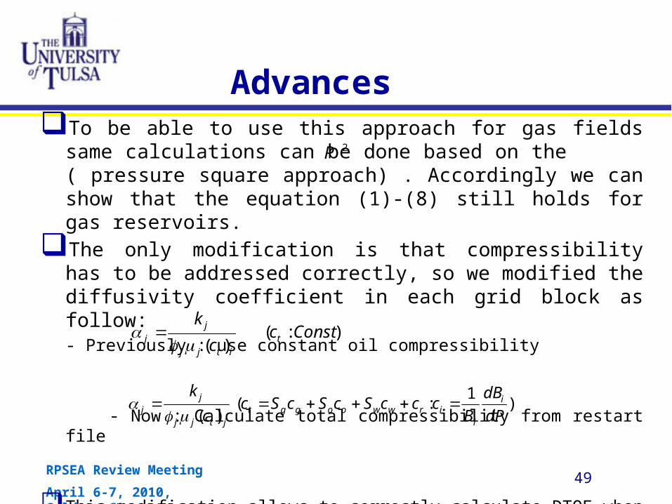
AdvancesTo be able to use this approach for gas fields same calculations

can be done based on the ( pressure square approach) . Accordingly we can show that the equation (1)-(8) still holds for gas reservoirs.

The only modification is that compressibility has to be addressed correctly, so we modified the diffusivity coefficient in each grid block as follow:- Previously : use constant oil compressibility

- Now : Calculate total compressibility from restart file

This modification allows to correctly calculate DTOF when multiple phases exist.

)1

:()( dP

dB

BcccScScSc

c

ki

iirwwooggt

jtjj

jj

):()(

Constcc

kt

itjj

jj

2P



Homogeneous Model

HeterogeneousModel

Diffusive TOF vs. Peak Time(2-D Single Phase GAS)

Diffusive TOF : DTOF

0.01 day

0.05 day

0.1 day

4

)(2

max

xt

P.A.T DTOF P.A.T



Field Case (Wamsutter Field- Tight Gas Reservoir) UPGRIDDING

Reduce the number of grid blocks from four million to about 700,000 (Faster Simulations)

Preserving the fine scale model dynamic behavior as good as possible.



Field Case (Wamsutter Field)

• Statistical Upgridding of the field

• We use Pressure Based Method upgridding (CONNECT – UpGrid)

• This method is based on combining layers with similar pressure profile and minimum velocity difference

• In Design Factor graph we use the maximum points. (Biggest contrast to proportional model)

Original Size : 98 × 112 × 361

= 3,962,336

Coarse scale Size : 98 × 112 × 65

= 713,440 (18% of original size)



Field Case (Wamsutter Field)

Section of the reservoir (18× 15× 65)

Original Size : 98 × 112 × 65

Permeability Field

(0.0001-3 md)



Section of Wamsutter Gas Field ( DTOF)

1 year



5 year

Section of Wamsutter Gas Field ( DTOF)



Drainage Volume Calculations

0 1,000 2,000 3,000 4,000 5,000 6,000 7,000 8,000 9,000 10,0000

2,000,000

4,000,000

6,000,000

8,000,000

10,000,000

12,000,000

14,000,000

2114721148

Time ( Days )

Dra

ina

ge

Vo

lum

e



Drainage Volume Calculations

0 1,000 2,000 3,000 4,000 5,000 6,000 7,000 8,000 9,000 10,0000

2,000,000

4,000,000

6,000,000

8,000,000

10,000,000

12,000,000

14,000,000

16,000,000

18,000,000

20,000,000

21147

21148

21147-Single Well

Incerement

Time ( Days )

Dra

inag

e V

olu

me



Field Case (Wamsutter Field- Tight Gas Reservoir)

Southwest Wyoming ( Number of the Wells : 85)

Permeability Field



Wamsutter Gas Field (Diffusive TOF)

25 year



Total Drainage Volume Calculations



Drainage Volume Whole Field

# 20222#

20032 # 20196



Well location and Streamlines

# 20032



Drainage Volume – # 20032



Summary

• We can use streamlines to visualize the pressure propagation in the gas reservoirs.

• Diffusive time of flight is a useful tool to calculate the pressure front.

• By calculating the drainage volume changes, we can quantify effect of new infill wells on the current producers.

• DTOF can facilitate the integration of the high resolution pressure data into history matching process.



Future Work

Optimized well placement based on the drainage volume

Optimized well completion based on the drainage volume

Including multi-stage fracturing

High resolution transient pressure history matching for

gas fields

rpsea review meeting april 6-7, 2010, golden, co 1 optimizing in fill well drilling - wamsutter...

Documents

rpsea review meeting

spacing slide

university slide

performance of wells

new wells

potential slide

wells methodology

wamsutter field slide