rough lecture notes
TRANSCRIPT
QUANTUM MECHANICS
Maciej Dunajski
Department of Applied Mathematics and Theoretical Physics
University of Cambridge
Wilberforce Road, Cambridge CB3 0WA, UK
AIMS, February 21, 2005
Abstract
These notes are based on a lecture course I gave to second and third year mathematics studentsat Oxford in years 1999–2002.
This is a mathematics course, and I am not assuming any knowledge of physics. Thecomments I will occasionally make about physics are there motivate some of the material, and(hopefully) make it more interesting.
The lectures will be self–contained but I need to assume some maths knowledge. In par-ticular I would want you to be familiar with basic concepts of linear algebra (like matrices,eigenvectors, eigenvalues, and diagonalisation), and ordinary differential equations (second or-der linear ODEs, boundary conditions).
Contents
1 The breakdown of classical mechanics 3
2 Schrodinger’s Equation 42.1 Separable solutions . . . . . . . . . . . . . . . . . . . . . . . . . . . . . . . . . . 42.2 The Interpretation of the wave function . . . . . . . . . . . . . . . . . . . . . . . 52.3 Conservation of probability . . . . . . . . . . . . . . . . . . . . . . . . . . . . . . 6
3 Basic scattering theory (in one dimension) 93.1 Free particle . . . . . . . . . . . . . . . . . . . . . . . . . . . . . . . . . . . . . . 93.2 Reflection and transmission coefficients . . . . . . . . . . . . . . . . . . . . . . . 103.3 Examples . . . . . . . . . . . . . . . . . . . . . . . . . . . . . . . . . . . . . . . 113.4 Potential Barrier . . . . . . . . . . . . . . . . . . . . . . . . . . . . . . . . . . . 113.5 Finite square well . . . . . . . . . . . . . . . . . . . . . . . . . . . . . . . . . . . 12
4 The harmonic oscillator 144.1 Hermite polynomials . . . . . . . . . . . . . . . . . . . . . . . . . . . . . . . . . 164.2 Correspondence with classical theory . . . . . . . . . . . . . . . . . . . . . . . . 174.3 2D oscillator . . . . . . . . . . . . . . . . . . . . . . . . . . . . . . . . . . . . . . 17
5 The hydrogen atom 195.1 The energy spectrum of the hydrogen atom . . . . . . . . . . . . . . . . . . . . . 195.2 Physical predictions . . . . . . . . . . . . . . . . . . . . . . . . . . . . . . . . . . 22
6 The mathematical structure of quantum theory 236.1 Hilbert spaces . . . . . . . . . . . . . . . . . . . . . . . . . . . . . . . . . . . . . 246.2 Linear operators . . . . . . . . . . . . . . . . . . . . . . . . . . . . . . . . . . . . 256.3 Postulates of quantum mechanics . . . . . . . . . . . . . . . . . . . . . . . . . . 276.4 Time evolution in QM . . . . . . . . . . . . . . . . . . . . . . . . . . . . . . . . 296.5 Commutation relations and canonical quantisation . . . . . . . . . . . . . . . . . 306.6 The Heisenberg uncertainty Principle . . . . . . . . . . . . . . . . . . . . . . . . 316.7 Commuting observables and parity . . . . . . . . . . . . . . . . . . . . . . . . . 32
7 The algebra of the harmonic oscillator 337.1 The harmonic oscillator once again . . . . . . . . . . . . . . . . . . . . . . . . . 35
1

8 Measurement and paradoxes 378.1 Measurement in quantum mechanics . . . . . . . . . . . . . . . . . . . . . . . . 378.2 The Einstein–Rosen–Podolsky paradoxes . . . . . . . . . . . . . . . . . . . . . . 388.3 Violation of Bell’s inequalities . . . . . . . . . . . . . . . . . . . . . . . . . . . . 388.4 Schrodinger’s cat . . . . . . . . . . . . . . . . . . . . . . . . . . . . . . . . . . . 40
2
Chapter 1
The breakdown of classical mechanics
Black body radiation: radiation emitted in packets (quanta)
E = ~ω, (1.1)
where ω is a frequency and ~ = 1.0546× 10⁻³⁴Js = h/2π is a Planck’s constant. (Planck 1900)Einstein 1905: The quanta are feature of light. Photo-electric effect:[PICTURE] Experimen-
tal fact: increasing of frequency of light increased the energy of emitted electrons, but not theirnumber. Increasing the flux (intensity) caused more electrons coming out with the same energy.Light is a stream of photons whose energy is proportional to the frequency ω = 2πc/γ, wherec is the speed of light and γ is the wavelength. 1900-1924 ‘Old quantum theory’ (Compton’sscattering, Nielst Bohr’s (1913) hydrogen atom). De Broglie waves (1924): particles (electrons)behave like waves:
p = ~k, (1.2)
where k is a wave vector |k| = 2π/γ.Particles in classical mechanics have well defined trajectories, that is a position, and a
velocity is known at each instant of time. How one might observe these features?[PICTURE]To measure particles position one must hit its with a photon, but this photon will transfer itsmomentum to a particle, thus changing particles momentum (it applies only to small particles,eg. electrons). Consequences
• Measurement process modifies what is being measured
• No trajectories in quantum mechanics
• Indeterminism (linked to the wave properties of matter)
Need for a new theory.
3
Chapter 2
Schrodinger’s Equation
Look for a wave equation satisfied by de Broglie ‘matter wave’. The plane wave ψ(x, t) =exp (−i(ωt− k · x) satisfies
i~∂ψ
∂t= ~ωψ = Eψ,
~i∇ψ = ~kψ = pψ.
Note the relationship between the observables (physical quantities which we want to measure)and differential operators acting on a wave function
E −→ i~∂
∂t, p −→ ~
i∇. (2.1)
For a conservative dynamical system H = p2/2m+ V (x) = E. Use (2.1) to obtain
i~∂ψ
∂t= − ~2
2m∇2ψ + V (x)ψ (2.2)
The time dependent Schrodinger equation (TDS) (1925) for a complex function ψ = ψ(x, t)(valid also in one or two dimensions). There are solutions other than plane waves.
2.1 Separable solutions
Look for ψ(x, t) = T (t)Ψ(x)
i~1
T
dT
dt=
1
Ψ
(− ~2
2m∇2Ψ + VΨ
)LHS = RHS =constant= E
i~dT
dt= ET −→ T (t) = e−itE/~T (0),
and−~2/2m∇2Ψ + VΨ = EΨ, (2.3)
which is the time independent Schrodinger equation (TIS). The stationary states are
ψ(x, t) = Ψ(x)T (0)e−itE/~ = ψ(x, 0)e−itE/~. (2.4)
4

2.2 The Interpretation of the wave function
What is ψ(x, t)? The most widely accepted is the (Copenhagen) interpretation in Max Born(1926):
• The entire information about a quantum state (particle) is contained in the wave function.For a normalised wave function
ρ(x) = |ψ(x)|2 = ψψ (2.5)
gives the probability density for the position of the particle.
So the probability that the particle moving on a line is in the interval (a, b) is given by∫ a
b
|ψ(x, t)|2dx. (2.6)
Remarks:
• Particle ‘has to be somewhere’, so∫R3
|ψ(x, t)|2d3x = 1 (2.7)
this is the normalisation condition.
• ψ(x, t) and ψ(x, t)eiφ(x,t) give the some information. The real function φ(x, t) is calledthe phase.
• Both (2.2) and (2.3) are linear differential equations. Their solutions satisfy the superpo-sition principle: If ψ1 and ψ2 are solutions then so is c1ψ1 + c2ψ2, for any c1, c2 ∈ C (sosolutions form a complex vector space, later to be identified with a Hilbert space.)
• The general solution to (2.2) will not be separable, but will be of the form∑cnψn(x, t), (2.8)
where ψn(x, t) = Ψn(x)Tn(t) are stationary states given by (2.4).
• For each stationary state
− ~2
2m∇2Ψn + VΨn = EnΨn.
The probability of measuring the value En is |cn|2, and (from the Parceval’s theorem, and(2.7)) [THINK ABOUT IT IN GENERAL]∑
n
|cn|2 = 1.
• The mean position is given by
〈r〉 =
∫R3
ψrψd3x
5
2.3 Conservation of probability
Assume the normalisation (2.7) at t = 0.∫R3
|ψ(x, 0)|2d3x = 1.
Is ∫R3
|ψ(x, t)|2d3x = 1 for t > 0 ?
The TDS equation (2.2) and its complex conjugations are
i~∂ψ
∂t= − ~2
2m∇2ψ + V (x)ψ,
−i~∂ψ∂t
= − ~2
2m∇2ψ + V (x)ψ,
where V (x) is real.
∂
∂t
(|ψ(x, t)|2
)=
∂ψ
∂tψ + ψ
∂ψ
∂t
=( ~
2im∇2ψ − V
i~ψ
)ψ + ψ
(− ~
2im∇2ψ +
V
i~ψ
)=
i~2m
(ψ∇2ψ − ψ∇2ψ) =i~2m
∇ · (ψ∇ψ − ψ∇ψ).
Definition 2.3.1 The probability current is
j(x, t) = − i~2m
(ψ∇ψ − ψ∇ψ). (2.9)
So we have proved
Proposition 2.3.2 If ψ is a solution to (2.2) then the probability density (2.5) and the proba-bility current (2.9) satisfy the continuity equation
∂ρ
∂t+ divj = 0. (2.10)
We shall now use the divergence theorem and Proposition 2.3.2 to show that QM probabilityis conserved.
Proposition 2.3.3 Suppose that j(x, t) tends to 0 faster than |x|−2 as |x| → ∞. Then∫R3
ρ(x, t)d3x.
is independent of time.
6
Proof. Let B be a ball enclosed by a sphere S|x| of radius |x|. Then
d
dt
∫B
ρ(x, t)d3x =
∫B
∂ρ(x, t)
∂td3x = −
∫B
divjd3x = −∫
S|x|
j · dS.
So if j(x, t) tends to 0 faster than |x|−2 the last integral tends to 0 as |x| → ∞, and so∫R3 ρ(x, t)d
3x is independent of time.
2
Example. Consider a potential well
V (x) =
0 for x ∈ (0, a)∞ otherwise.
(2.11)
The equation (2.3) reduces to
− ~2
2m
d2Ψ
dx2= EΨ for x ∈ (0, a), Ψ = 0 otherwise.
Solve the boundary value problem
Ψ(x) =
A cosh(x√
2m|E|/~) +B sinh(x√
2m|E|/~) if E < 0A+Bx if E = 0
A cos(x√
2mE/~) +B sin(x√
2mE/~) if E > 0.
From Ψ(0) = 0 we have A = 0 in each case. From Ψ(a) = 0 we have B = 0 if E 6 0 (so thatΨ = 0 in those cases), and
a√
2mE
~= nπ for n ∈ Z if E > 0.
So we have infinitely many nontrivial solutions parametrised by a positive integer (the sign canbe absorbed in B)
Ψn(x) = Bn sin(nπx
a
), and En =
n2π2~2
2ma2. (2.12)
Remarks
• Equation (2.3) gave rise to an eigenvalue problem. Allowed energies are eigenvalues En
corresponding to eigenvectors Ψn. If a given eigenvalue corresponds to only one eigenvec-tor then it is called non-degenerated. Otherwise it is degenerated
• Energies of the system can take only discrete values, which is a purely quantum phe-nomenon.
Definition 2.3.4 When the energies of a quantum system are discrete and bounded below, thenthe lowest possible energy state is called the ground state and the higher states are known as 1st,2nd, ..., kth excited states. The integer parametrising discrete energies (or other observables)is called a quantum number.
7
The normalisation condition (2.7) yields∫ a
0
Bn2 sin2
(nπxa
)dx = 1, so Bn =
√2
a.
The stationary states (2.4) are
ψn(x, t) =
√2
ae−in2π2~t/(2ma2) sin
nπx
a
and the general solution is given by (2.8). To determine cn suppose that ψ(x, 0) = f(x). From(2.8)
f(x) =
√2
a
∞∑n=1
cn sinnπx
a, so cn =
√2
a
∫ a
0
f(x) sinnπx
adx. (2.13)
Look at Born’s probabilistic interpretation:
|ψn(x, t)|2 =2
asin2 nπx
a=
1
a
(1− cos
2nπx
a
).
What is a probability that a particle described by ψn is between 0 and x0?
Fn(x0) =
∫ x0
0
1
a
(1− cos
2nπx
a
)dx =
(x0
a− 1
2nπsin
2nπx0
a
).
The classical distribution would be F (x0) = x0/a = limn→∞ Fn(x0).
Definition 2.3.5 (Bohr’s correspondence principle) Quantum mechanical formulae ap-proach those of the classical mechanics if the quantum number is large.
Example 2.3.6 Suppose that ψ(x, 0) = 1/√a = const. Find a probability of measuring energy
En.
From (2.13)
cn =
√2
a
∫ a
0
√1
asin
nπx
adx =
√2
nπ
[− cos
nπx
a
]a
0=
√2
nπ[1− (−1)n]
So the probability of measuring En is 0 if n is even, and
8
n2π2
if is n is odd.
8
Chapter 3
Basic scattering theory (in onedimension)
The way physicists discover new elementary particles is by scattering experiments. Huge accel-erators collide particles through targets, and by analysing the changes to momentas of scatteredparticles, a picture of a target is built. We shall look at some features of the scattering theory.
3.1 Free particle
Equation (2.3) with V = 0 yields
− ~2
2m
d2Ψ
dx2= EΨ.
With the definition k =√
2mE/~ the solution is
Ψ(x) = Aeikx +Be−ikx, (3.1)
and the stationary states (2.4) are
ψ(x, t) = Ψ(x)e−iEt/~ = Aei(kx−ωt)︸ ︷︷ ︸incoming wave
+ Be−i(kx+ωt)︸ ︷︷ ︸outgoing wave
, where ω =E
~. (3.2)
Convention: incoming=incident from the left.
Remarks
• If B = 0, then ρ(x, t) = |ψ(x, t)|2 = |A|2, so the probability of finding a particle in aninterval L is (from (2.6)) |A|2L. But∫
Rρ(x, t)dx = ∞,
and the plane waves can not be normalised (one way to get around it is suggested in theproblem one, sheet two). However it still makes sense to talk about relative probabilitiesof finding a particle in two intervals.
9
• The normalizable wave functions (like (2.12)) are called bound states. Other (like planewaves (3.2) ) are scattering states.
• There are no restrictions on k (and so E) in (3.2). Therefore the energies are continuous.
• The probability current (2.9) for (3.2) is
j =~
2mi
(ψ
dψ
dx− ψ
dψ
dx
)=
~km
(|A|2 − |B|2
), (3.3)
where the factor ~k/m can be identified (by the De Broglie formula (1.2)) with a velocity.
3.2 Reflection and transmission coefficients
In the example (2.11) the boundary conditions at ∞ determined the energy eigenvalues in(0, a) (this led to a discrete spectrum). In the scattering theory the energy of a potentialbarrier determines energies of a quantum system at the large distances. [PICTURE] Regionswhere V (x) = 0 correspond to free particle (3.1)
Ψ(x) =
ΨL = ALe
ikLx +BLe−ikLx, for x 6 0
ΨV depends on V (x), for x ∈ [0, a]ΨR = ARe
ikRx, for x > a
For a beam incident from the left define
Definition 3.2.1
Reflection coefficient =|reflected current||incident current|
=|BL|2
|AL|2= R
Transmission coefficient =|transmitted current||incident current|
=kR|AR|2
kL|AL|2= T (3.4)
We don’t know Ψ in the interaction region. However, we can still say something:
Proposition 3.2.2 For one-dimensional, time independent problems
1. The probability current is constant.
2. The sum of reflection and transmition coefficient is 1.
Proof.
1. The continuity equation (2.10) reduces to dj/dx = 0, so that j is constant in regions L, V ,and R. In fact jL = jV = jR, which follows from the matching conditions: Ψ and dΨ/dxare continuous at x = 0 and x = a (and in general, at the potential discontinuities), sothat the probability current is well defined.
2. Equation (3.3) and the first part of this Proposition imply
kL(|AL|2 − |BL|2) = kR|AR|2.
The result follows if one divides the last formula by kL|AL|.
2
10
3.3 Examples
Potential Step [PICTURE]
V (x) =
0 for x < 0V0 for x > 0.
(3.5)
Ψ =
ΨL = ALe
ikLx +BLe−ikLx, for x < 0, where kL =
√2mE/~
ΨR = AReikRx +BRe
−ikRx, for x > 0, where kR =√
2m(E − V0)/~.
Note that kR may be real or imaginary. The matching conditions are
ΨL(0) = ΨR(0) −→ AL +BL = AR +BR
Ψ′L(0) = Ψ′
R(0) −→ kL(AL −BL) = kR(AR −BR),
which relates the waves on both sides of the potential jump
AL =1
2kL
((kL + kR)AR + (kL − kR)BR
),
BL =1
2kL
((kL − kR)AR + (kL + kR)BR
).
Assume that the particle is incident from the left, and E > V0. Now kR is real and BR = 0 (asno beam is coming from ∞. The reflection and transmition coefficients (scattering data) aregiven by
R =|BL|2
|AL|2=
(kL − kR)2
(kL + kR)2, T =
kR|AR|2
kL|AL|2=
4kLkR
(kL + kR)2.
3.4 Potential Barrier
[PICTURE]
V (x) =
V0 > 0 for x ∈ [0, a]0 otherwise.
(3.6)
Consider an incoming beam of particles with energy 0 < E < V0. In classical mechanics thewhole beam would be reflected. How about QM? In the regions 0 and 2 we have the free particlesolutions (3.1). In the region 1 the wave function satisfies
d2Ψ
dx2− k2Ψ = 0, where k=
√2m(V0 − E)
~.
Therefore we have
Ψ =
Ψ0 = A0e
ikx +B0e−ikx, for x 6 0 k =
√2mE/h
Ψ1 = A1ekx +B1e
−kx, for x ∈ [0, a]Ψ2 = A2e
ikx, for x > a
11
B2 = 0 as there are no incident particles coming from from ∞. Continuity of the wave functionand its first derivatives gives four conditions on five constant
Ψ0(0) = Ψ1(0) A0 +B0 = A1 +B1
Ψ0′(0) = Ψ1
′(0) ik(A0 −B0) = k(A1 +B1)
Ψ1(a) = Ψ2(a) A1eak +B1e
−ak = A2eika
Ψ1′(a) = Ψ2
′(a) k(A1eak −B1e
−ak) = ikA2eika.
A simple algebra givesA2
A0
=4ikke−ika
eka(k + ik)2 − e−ka(k − ik)2
so that the transmition coefficient (3.4) T 6= 0. This is a quantum phenomenon known astunnelling. Classical particles with E < V0 would not have enough energy to penetrate tebarrier. Quantum particles can (because of their wave properties) tunnel through large barriers.This has many application (for example Scanning tunneling electron microscope, Nobel 1986).
3.5 Finite square well
[PICTURE]
V (x) =
0 for x ∈ (0, a)V0 > 0 otherwise.
(3.7)
Case 1. 0 < E < V0 [Bound states.] In the region x ∈ (0, a)
d2Ψ
dx2+ k2Ψ = 0, where k =
√2mE
~.
In the region x ∈ (−∞, 0] ∪ [a,∞)
d2Ψ
dx2− k2Ψ = 0, where k =
√2m(V0 − E)
~.
This yields
Ψ =
Ψ0 = A0e
kx, for x 6 0Ψ1 = A1e
ikx +B1e−ikx, for x ∈ [0, a]
Ψ2 = B2e−kx, for x > a
and B0 = A2 = 0 so that Ψ remains bounded for |x| → ∞. We have four boundary conditions:
A0 − A1 −B1 = 0
kA0 − ikA1 + ikB1 = 0
eikaA1 + e−ikaB1 − e−kaB2 = 0
ikeikaA1 − ike−ikaB1 + ke−kaB2 = 0
12
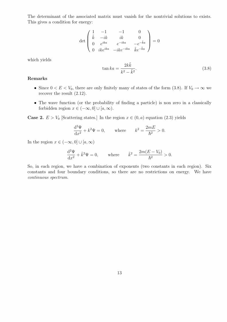
The determinant of the associated matrix must vanish for the nontrivial solutions to exists.This gives a condition for energy:
det
1 −1 −1 0
k −ik ik 0
0 eika e−ika −e−ka
0 ikeika −ike−ika ke−ka
= 0
which yields
tan ka =2kk
k2 − k2. (3.8)
Remarks
• Since 0 < E < V0, there are only finitely many of states of the form (3.8). If V0 →∞ werecover the result (2.12).
• The wave function (or the probability of finding a particle) is non zero in a classicallyforbidden region x ∈ (−∞, 0] ∪ [a,∞).
Case 2. E > V0 [Scattering states.] In the region x ∈ (0, a) equation (2.3) yields
d2Ψ
dx2+ k2Ψ = 0, where k2 =
2mE
~2> 0.
In the region x ∈ (−∞, 0] ∪ [a,∞)
d2Ψ
dx2+ k2Ψ = 0, where k2 =
2m(E − V0)
~2> 0.
So, in each region, we have a combination of exponents (two constants in each region). Sixconstants and four boundary conditions, so there are no restrictions on energy. We havecontinuous spectrum.
13

Chapter 4
The harmonic oscillator
In classical mechanics the harmonic oscillator is described by the potential V = (1/2)mω2x2,which leads to the Newton equation
d2x
dt2= −mω2x,
and the continuous energy spectrum.The quantum harmonic oscillator (first solved by Heisenberg in 1925) is an important ex-
ample, because many systems (eg. atoms in crystals) undergoing small disturbances behavelike harmonic oscillators. The time independent Schrodinger equation (2.3) yields
− ~2
2m
d2Ψ
dx2+
1
2mω2x2Ψ = EΨ. (4.1)
We shall adopt the following strategy:
1. Find the asymptotic behaviour φ of Ψ for large |x|,
2. make a substitution Ψ = fφ,
3. solve an equation for f using a power series method (a1 differential equations).
First simplify: In terms ofz := x
√mω/~, ε = E/~ω
equation (4.1) becomes
Ψ′′ + (2ε− z2)Ψ = 0, where ′ =d
dz. (4.2)
Step 1: For large z the function φ = exp (−z2/2) satisfies (4.2). Inspection
φ′ = −zφ, φ′′ = −φ+ z2φ, (4.3)
which is (4.2) with ε = 1/2. For large z the multiple of z2 dominates, so we neglect ε.Step 2: Substitute Ψ(z) = f(z)φ(z) to (4.2)
f ′′φ+ 2f ′φ′ + fφ′′ + (2ε− z2)fφ = 0.
14
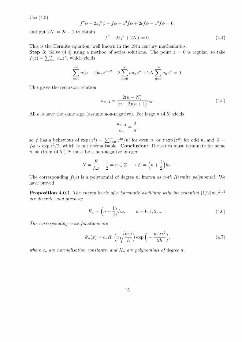
Use (4.3)f ′′φ− 2zf ′φ− fφ+ z2fφ+ 2εfφ− z2fφ = 0,
and put 2N := 2ε− 1 to obtainf ′′ − 2zf ′ + 2Nf = 0. (4.4)
This is the Hermite equation, well known in the 19th century mathematics.Step 3: Solve (4.4) using a method of series solutions. The point z = 0 is regular, so takef(z) =
∑∞n=0 anz
n, which yields
∞∑n=0
n(n− 1)anzn−2 − 2
∞∑n=0
nanzn + 2N
∞∑n=0
anzn = 0.
This gives the recursion relation
an+2 =2(n−N)
(n+ 2)(n+ 1)an. (4.5)
All ans have the same sign (assume non-negative). For large n (4.5) yields
an+2
an
=2
n,
so f has a behaviour of exp (z2) =∑∞
n=0 z2n/n! for even n, or z exp (z2) for odd n, and Ψ =
fφ ∼ exp z2/2, which is not normalisable. Conclusion: The series must terminate for somen, so (from (4.5)) N must be a non-negative integer
N =E
~ω− 1
2= n ∈ Z −→ E =
(n+
1
2
)~ω.
The corresponding f(z) is a polynomial of degree n, known as n-th Hermite polynomial. Wehave proved
Proposition 4.0.1 The energy levels of a harmonic oscillator with the potential (1/2)mω2x2
are discrete, and given by
En =(n+
1
2
)~ω, n = 0, 1, 2, ... . (4.6)
The corresponding wave functions are
Ψn(x) = cnHn
(x
√mω
~
)exp
(− mωx2
2~
), (4.7)
where cn are normalisation constants, and Hn are polynomials of degree n.
15

4.1 Hermite polynomials
Equation (4.4) with N integer is
Hn′′ − 2zHn
′ + 2nHn = 0, n = 0, 1, ... . (4.8)
This defines Hn up to a multiplicative constant, which is fixed by demanding that the coefficientof zn in Hn(z) is 2n. The first few polynomials are
H0(z) = 1, H1(z) = 2z, H2(z) = 4z2 − 2, H3(z) = 8z3 − 12z, ...
From (4.5) it follows that Hn is even for even n, and odd for odd n. The general form ofHermite polynomials is given by
Proposition 4.1.1 Let Hn be a polynomial of degree n which satisfies (4.8), and is normalisedby demanding that the coefficient of zn in Hn(z) is 2n. Then
Hn(z) = (−1)nez2( d
dz
)n
e−z2
. (4.9)
Proof. Define a generating function
G(z, s) =∞∑
n=0
sn
n!Hn(z)
so that
Hn(z) =( ∂
∂s
)n
G(z, s)|s=0.
One can show (sheet 3, problem 4), that
G(z, s) = e−s2+2sz. (4.10)
The last formula will give the general form of Hermite polynomials. Rewrite (4.10) as G(z, s) =exp (z2) exp [−(s− z)2], and note that
∂
∂sexp [−(s− z)2] = −2(s− z) exp [−(s− z)2] = − ∂
∂zexp [−(s− z)2].
Therefore
Hn(z) = (−1)nez2( ∂
∂z
)n
e−(s−z)2|s=0 = (−1)nez2( d
dz
)n
e−z2
.
2
We shall now use (4.9) to determine the normalisation constants cn appearing in (4.7)
1 =
∫ ∞
−∞|Ψn|2dx =
√~mω
∫ ∞
−∞|cn|2[Hn(z)]2e−z2
dz =
√~mω
|cn|2∫ ∞
−∞(−1)nHn(z)
( d
dz
)n
e−z2
dz.
We integrate the last formula n times by parts, and note that exp (−z2) vanishes at ±∞. Thisyields
1 =
√~mω
|cn|2∫ ∞
−∞e−z2
( d
dz
)n
Hn(z)dz,
16
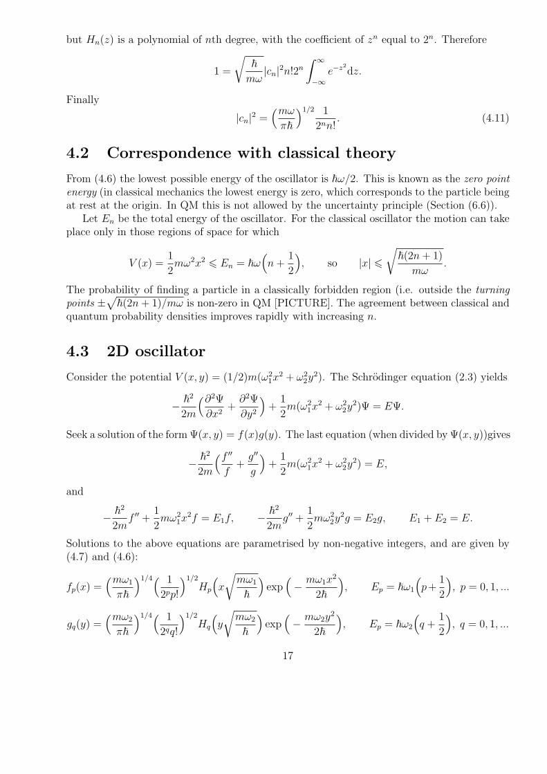
but Hn(z) is a polynomial of nth degree, with the coefficient of zn equal to 2n. Therefore
1 =
√~mω
|cn|2n!2n
∫ ∞
−∞e−z2
dz.
Finally
|cn|2 =(mωπ~
)1/2 1
2nn!. (4.11)
4.2 Correspondence with classical theory
From (4.6) the lowest possible energy of the oscillator is ~ω/2. This is known as the zero pointenergy (in classical mechanics the lowest energy is zero, which corresponds to the particle beingat rest at the origin. In QM this is not allowed by the uncertainty principle (Section (6.6)).
Let En be the total energy of the oscillator. For the classical oscillator the motion can takeplace only in those regions of space for which
V (x) =1
2mω2x2 6 En = ~ω
(n+
1
2
), so |x| 6
√~(2n+ 1)
mω.
The probability of finding a particle in a classically forbidden region (i.e. outside the turningpoints ±
√~(2n+ 1)/mω is non-zero in QM [PICTURE]. The agreement between classical and
quantum probability densities improves rapidly with increasing n.
4.3 2D oscillator
Consider the potential V (x, y) = (1/2)m(ω21x
2 + ω22y
2). The Schrodinger equation (2.3) yields
− ~2
2m
(∂2Ψ
∂x2+∂2Ψ
∂y2
)+
1
2m(ω2
1x2 + ω2
2y2)Ψ = EΨ.
Seek a solution of the form Ψ(x, y) = f(x)g(y). The last equation (when divided by Ψ(x, y))gives
− ~2
2m
(f ′′f
+g′′
g
)+
1
2m(ω2
1x2 + ω2
2y2) = E,
and
− ~2
2mf ′′ +
1
2mω2
1x2f = E1f, − ~2
2mg′′ +
1
2mω2
2y2g = E2g, E1 + E2 = E.
Solutions to the above equations are parametrised by non-negative integers, and are given by(4.7) and (4.6):
fp(x) =(mω1
π~
)1/4( 1
2pp!
)1/2
Hp
(x
√mω1
~
)exp
(− mω1x
2
2~
), Ep = ~ω1
(p+
1
2
), p = 0, 1, ...
gq(y) =(mω2
π~
)1/4( 1
2qq!
)1/2
Hq
(y
√mω2
~
)exp
(− mω2y
2
2~
), Ep = ~ω2
(q +
1
2
), q = 0, 1, ...
17
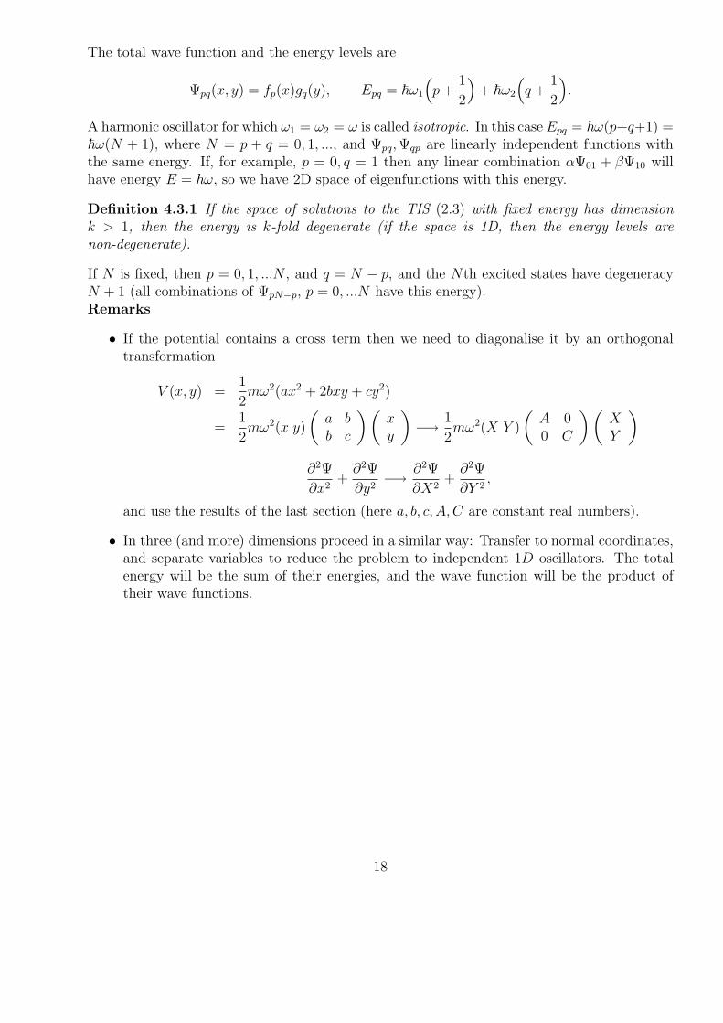
The total wave function and the energy levels are
Ψpq(x, y) = fp(x)gq(y), Epq = ~ω1
(p+
1
2
)+ ~ω2
(q +
1
2
).
A harmonic oscillator for which ω1 = ω2 = ω is called isotropic. In this case Epq = ~ω(p+q+1) =~ω(N + 1), where N = p + q = 0, 1, ..., and Ψpq,Ψqp are linearly independent functions withthe same energy. If, for example, p = 0, q = 1 then any linear combination αΨ01 + βΨ10 willhave energy E = ~ω, so we have 2D space of eigenfunctions with this energy.
Definition 4.3.1 If the space of solutions to the TIS (2.3) with fixed energy has dimensionk > 1, then the energy is k-fold degenerate (if the space is 1D, then the energy levels arenon-degenerate).
If N is fixed, then p = 0, 1, ...N , and q = N − p, and the Nth excited states have degeneracyN + 1 (all combinations of ΨpN−p, p = 0, ...N have this energy).Remarks
• If the potential contains a cross term then we need to diagonalise it by an orthogonaltransformation
V (x, y) =1
2mω2(ax2 + 2bxy + cy2)
=1
2mω2(x y)
(a bb c
) (xy
)−→ 1
2mω2(X Y )
(A 00 C
) (XY
)∂2Ψ
∂x2+∂2Ψ
∂y2−→ ∂2Ψ
∂X2+∂2Ψ
∂Y 2,
and use the results of the last section (here a, b, c, A, C are constant real numbers).
• In three (and more) dimensions proceed in a similar way: Transfer to normal coordinates,and separate variables to reduce the problem to independent 1D oscillators. The totalenergy will be the sum of their energies, and the wave function will be the product oftheir wave functions.
18
Chapter 5
The hydrogen atom
Ernesrt Rutherford [1911] (based on experiments): atoms are miniatures of solar systems.Electrons of charge −e orbit heavy (fixed) nucleus of a positive charge Ze [PICTURE]. Fora hydrogen atom we have one electron. Classically atoms should not exist: Moving electronsradiate the electromagnetic energy, and fall into a nucleus. The first QM explanation was givenby Bohr [1913] (using ad-hoc assumptions), and latter by Pauli [1925]. This was one of thebiggest successes of quantum theory.
Force acting on electron [PICTURE]
F (r) =−Ze2
4πε0r2.
The corresponding potential
V (r) =−Ze2
4πε0r
(compare the Newtonian gravity, Mods TT), where r is the distance between the electron andnucleus, ε0 = const (dielectric constant of vacuum), and m is the mass of the electron. The 3DTIS is
− ~2
2m∇2Ψ− Ze2
4πε0rΨ = EΨ. (5.1)
LECTURE 8
5.1 The energy spectrum of the hydrogen atom
We shall neglect the angular variables, and assume that the electron moves radially in thecentral potential. This will be sufficient to determine the energy levels. The full treatmentinvolving the angular variables leads to spherical harmonics, and will be discussed in the courseFurther Quantum Theory. If Ψ = Ψ(r), then (5.1) becomes
−~2
2m
1
r
d2
dr2(rΨ)− Ze2
4πε0rΨ = EΨ.
Define
R = rΨ, and α =4πε0~2
Zme2, (5.2)
19
and rewrite the last equation as
d2
dr2R +
2
αrR +
2mE
~2R = 0. (5.3)
We aim to solve this equation subject to the following boundary conditions:
• Ψ = R/r is finite at r = 0, so limr→0R(r) = 0,
•∫
R3 |Ψ(r)|2r2dr is finite, so limr→∞R(r) = 0.
Our strategy will be similar to the one we used to solve the harmonic oscillator.Step 1: For large r the asymptotic behaviour is
d2
dr2R +
2mE
~2R ' 0,
so the energy is negative (otherwise we would have the oscillatory solution contradicting thesecond boundary condition). With the definition k2 = −2mE/~2 we have R ' exp (−kr), forlarge r.Step 2: Set R(r) = f(r) exp (−kr). Equation (5.3) yields
k2e−krf − 2ke−kr df
dr+ e−kr d2f
dr2+
2
αre−krf − k2e−krf = 0.
Put ρ = r/α. Then the last equation becomes
d2
dρ2f − 2kα
d
dρf +
2
ρf = 0. (5.4)
Now ρ = 0 is a ‘regular singular point’, so look for a solution of the form
f(ρ) = ρc
∞∑n=0
anρn.
Equation (5.4) yields
∞∑n=0
(n+ c)(n+ c− 1)anρn+c−2 − 2kα
∞∑n=0
(n+ c)anρn+c−1 + 2
∞∑n=0
anρn+c−1.
Setting n = 0 we obtain the indicial equation c(c− 1) = 0. Its solutions differ by integer. Wetake c = 1 (because R/r must be finite at r = 0). The recurrence equation is
n(n+ 1)an = 2(kαn− 1)an−1. (5.5)
Now argue as for the harmonic oscillator. For large n
an
an−1
' 2kα
n,
20
and f behaves like exp (2kαρ) = exp (2kr) (so Ψ is not normalizable). Therefore the seriesmust terminate, and
kαn− 1 = 0, for some n = 1, 2, ... .
Recall that k2 = −2mE/~2, so the energy levels are
En =−k2~2
2m= − ~2
2mα2n2=E1
n2. (5.6)
The energies are negative because it is conventional to take V = 0 at ∞.
Definition 5.1.1 The positive integer n is known as the principal quantum number.
The radial wave function with principal quantum number n is
Ψn(r) =e−kr
rf(r) = e−r/αn[a0 + a1(r/α) + ..an−1(r/α)(n−1)] = e−r/αnLn(r/α), (5.7)
where Ln is a polynomial of order n− 1 [CHECK], called the Laguerre polynomial.
Example 5.1.2 Let us normalise the ground state Ψ1(r) = a0 exp [−(r/α)] (corresponding ton = 1)
1 =
∫R3
|Ψ1(r)|r2 sin θdrdθdφ = 4π|a0|2∫ ∞
0
r2e−2r/αdr.
Instead of integrating it by parts we shall perform a simple trick (often used by Richard Feyn-man). Put β = 2/α. Then
1 = 4π|a0|2d2
dβ2
∫ ∞
0
e−βrdr = 4π|a0|2d2
dβ2
[− 1
βe−βr
]∞0
=8π|a0|2
β3= π|a0|2α3,
and
Ψ1(r) =1√πα3
e−r/α, (5.8)
where α is given by (5.2).
The probability of the electron being in the spherical shell between r and r+dr is 4π|Ψn(r)|2r2dr.The radial probability density for Ψ1
r2e−2r/α
has a maximum at r = α[PICTURE]. The constant α is therefore the most probable radialdistance of the electron from the nucleus (if Z = 1 the number α is called the Bohr radius).The expectation value of r for the ground state is
< r >= 4π
∫ ∞
0
ΨirΨ1r2dr =
3α
2.
21
5.2 Physical predictions
• For large n we have En → 0, the minimum energy to escape the nucleus. The case E > 0corresponds to scattering states.
• Suppose that the electron jumps from level Ej to Ek (k > j). This releases energy
Ej − Ek = Ejk =( 1
j2− 1
k2
)E1 = ~ωjk, (5.9)
(where we used the Planck law (1.1), and (5.6)), in the form of light (a photon). (Forj = 2 frequencies (5.9) are in visible part of electro-magnetic spectrum, called the Balmerseries. They have been measured, and provide an excellent experimental test of QM). Ifan electron absorbs a photon the reverse process occurs, and the electron can jump up alevel (excitation). If an energy of an absorbed photon is large enough, the electron mayescape from the atom. If an electron occurs in the state Ej, the photon must supply −Ej
(ionization energy).
• The ‘solar system’ analogy is not good. A ‘cloud’ is (the electron spreads over a wholeatom, until measured).
22
Chapter 6
The mathematical structure ofquantum theory
Imagine a thought experiment: Particle in a box[PICTURE]. We do not know where it is ,so the wave function must be spread throughout the box. An impenetrable membrane in nowinserted dividing the box into two disconnected chambers 1, and 2. Some of the wave is trappedin 1, some in 2, but the particle is only in one chamber. If an observation is made, and theparticle is found in 1, then the wave in chamber 2 must disappear - there is a zero probabilityof finding a wave in 2. This is called a collapse of the wave function and will be discussed inSection 8. Before the observation
Ψ = c1Ψ1 + c2Ψ2
such that Ψ1 = 0 in chamber 2, and Ψ2 = 0 in chamber 1. We have∫chamber 1
|Ψ1|2dV = 1 =
∫chamber 2
|Ψ2|2dV.
The normalisation condition
1 =
∫box
|Ψ|2dV = |c1|2 + |c2|2︸ ︷︷ ︸1
+ 2Re[c1c2
∫box
Ψ1Ψ2dV ]
gives the orthogonality relation ∫box
Ψ1Ψ2dV = 0.
This example generalizes to many (or infinitely many) chambers: Now
Ψ =∑
n
cnΨn, (6.1)
where Ψn is a normalised wave function in chamber n and the summation is over all chambers.From the normalisation condition we deduce the orthogonality relations∫
box|Ψ|2dV = 1 −→
∫box
ΨmΨndV = δnm =
1 if m = n0 if m 6= n,
(6.2)
23
where δnm is the Kronecker tensor. Analogies with the linear algebra of vectors (a1) are clear:Equation (6.1) is an expansion of a vector Ψ in an orthogonal basis Ψn, and equation (6.2)defines a scalar (or inner) product. The orthogonality reflects the exclusive property of mea-surement.
6.1 Hilbert spaces
Following Paul Dirac (19??) we shall denote the state vectors by
|Ψ〉 ∈ H ‘ket’ vectors, and 〈Φ| ∈ H∗ ‘bra’ vectors.
Here H is a complex vector space with an inner product (unitary space), H∗ is its dual. The(anti-)isomorphism between H and H∗ is
|Ψ〉 =∑N
cn|Ψn〉 ∼ 〈Ψ| =∑N
cn〈Ψn|, where cn ∈ C. (6.3)
The scalar product is(〈Φ|, |Ψ〉) ∈ H∗ ×H −→ 〈Φ|Ψ〉︸ ︷︷ ︸
bra-ket
∈ C. (6.4)
The norm in H is defined by:
‖Ψ‖2 = 〈Ψ|Ψ〉 (= 1 for normalised states). (6.5)
The properties of the scalar product are
〈Φ|Ψ〉 = 〈Ψ|Φ〉 (6.6)
〈Φ|(α|Ψ〉+ β|Θ〉) = α〈Φ|Ψ〉+ β〈Φ|Θ〉, (6.7)
and they imply(〈αΦ|+ 〈βΩ|)|Θ〉 = α〈Φ|Θ〉+ β〈Ω|Θ〉,
for any α, β ∈ C, |Ψ〉, |Θ〉 ∈ H, 〈Φ|, 〈Ω| ∈ H∗. Note that the QM conventions are other wayaround to the algebraic conventions; The inner product is linear in a second variable andanti-linear in a first.
The vector space H is usually infinite. We shall assume that it is complete in the followingsense: Whenever |Ψn〉 ∈ H is a sequence of vectors, such that
∀ε>0∃Nε∈Z‖Ψn〉 − |Ψm〉| < ε for all m,n > Nε
than there exists a limit vector |Ψ〉 ∈ H, such that ‖Ψn〉−|Ψ〉| −→ 0 (i.e. any Cauchy sequencein H is convergent).
Definition 6.1.1 A Hilbert space is a complex inner product space which is complete.
The state space is assumed to be a Hilbert space (strictly speaking a Hilbert space is ‘to small’to contain the eigenstates of position and momentum operators. Instead, one uses a space oftempered distributions).
24
Example 6.1.2 H = L2(Rn) (where n = 1, 2, 3 are important cases) is a space of complex-valued functions such that
‖f‖2 =
∫Rn
|f(x)|2dnx <∞. (6.8)
This example is very important in wave mechanics. In fact we used it in the first half of thecourse. The scalar product is given by
〈f |g〉 =
∫Rn
fgdnx. (6.9)
It is well defined as a consequence of (6.8).
Example 6.1.3 H = Cn. Let
|f〉 =
f1...fn
, |g〉 =
g1...gn
, where fi, gi ∈ C.
The scalar product is
〈f |g〉 =n∑
i=1
f igi ∈ C. (6.10)
6.2 Linear operators
Observables in QM are described by certain linear transformations. Let A : H −→ H be alinear operator (transformation) on H, i.e.
A(α|Ψ〉+ β|Φ〉) = αA|Ψ〉+ βA|Φ〉 (6.11)
where α, β ∈ C. The linear operators (from now on called just operators) can be added andmultiplied:
(αA+ βB)|Ψ〉 = αA|Ψ〉+ βB|Ψ〉, (AB)|Ψ〉 = A(B|Ψ〉).Therefore they form an associative algebra. Note that an operator A may be defined only on asubspace D(A) of H, called the domain of A.
Definition 6.2.1 The commutator of two operators A, B is
[A, B] := AB − BA. (6.12)
The commutators do not usually vanish, so operator algebras are non-commutative. Propertiesof commutators:
Proposition 6.2.2 For operators all A, B, C, the commutator satisfies
[A, B] = −[B, A] (6.13)
[αA+ βB, C] = α[A, C] + β[B, C] (6.14)
[A, BC] = B[A, C] + [A, B]C (Leibnitz rule) (6.15)
[A, [B, C]] + [B, [C, A]] + [C, [A, B]] = 0 (Jacobi identity). (6.16)
25

Proof. Similar to identities for Poisson brackets.
2
Remark A vector space (for example of operators) equipped with bi-linear product satisfying(6.13), (6.14), and (6.16) is called Lie algebra.
Definition 6.2.3 The adjoint of a linear operator A is the unique linear transformation A∗
that satisfies(〈Φ|A∗)|Ψ〉 = 〈Φ|(A|Ψ〉) (6.17)
for all |Ψ〉, |Φ〉 ∈ D(A). The operator is called self-adjoint (or incorrectly Hermitian in thephysics literature) if A = A∗.
Remark. We shall usually rewrite formula (6.17) as 〈A∗Φ|Ψ〉 = 〈Φ|AΨ〉. Formulae (6.6,6.17)imply
〈Ψ|A∗Φ〉 = 〈AΨ|Φ〉 = 〈Φ|AΨ〉.For self-adjoint operators it makes sense to write 〈Φ|A|Ψ〉.
Definition 6.2.4 Let |Ψ〉 6= 0 be a vector such that
A|Ψ〉 = a|Ψ〉 (6.18)
for some a ∈ C. Then |Ψ〉 is called an eigen-vector and a is called an eigen-value of A.
Example 6.2.5 Let H = L2(Rn) be the Hilbert space from the Example 6.1.2. Now |f〉 =f(x1, ..., xn). Examples of operators are
X1f := x1f D1f :=∂f
∂x1
, 1f := f.
These are multiplication operator, differentiation operator, and identity operator respectively.There are many more examples. Note that
D1(X1f)− X1(D1f) = (D1(x1))f, so [D1, X1] = 1.
Example 6.2.6 Let H = Cn be the Hilbert space from the Example 6.1.3.
A|f〉 =
A11 . . . A1n...
. . ....
An1 . . . Ann
f1
...fn
,
so linear operators are represented by n×n complex matrices. What is the matrix correspondingto A∗? Let |f〉, |g〉 ∈ Cn. The formula
〈A∗f |g〉 = 〈f |Ag〉
has the following matrix counterpart
n∑i,j
(A∗ijf j)gi =
n∑i,j
f i(Aijgj).
26
Changing i to j in the RHS, and comparing coefficients of fjgi we find that
A∗ = AT
(6.19)
The matrix A∗ is called a Hermitian conjugate of A. Hermitian matrices are those for whichA∗ = A. In the finite-dimensional case the self-adjoint operators are represented by Hermitianmatrices.
6.3 Postulates of quantum mechanics
Wave mechanics of Schrodinger was preceded by a matrix mechanic of Heisenberg (1925). Thegeneral mathematical scheme containing both mechanics as special cases was later proposed byvon-Neumann, Weyl, Wigner and others.
1. Each physical system is described by an element of a Hilbert space H (a state vector),which contains all information about the system.
2. Superposition principle. If |Ψ1〉, and |Ψ2〉 are state vectors then α|Ψ1〉 + β|Ψ2〉 (forα, β ∈ C) is also a possible state vector.
3. The observables (dynamical variables, like position, momentum, energy, ...) are repre-sented by self-adjoint operators in H.
4. The result of measuring an observable (corresponding to) A is one of the eigenvalues ofA. If a state vector is
|Ψ〉 =∑
n
cn|Ψn〉, (6.20)
where |Ψn〉s are eigen-vectors of A ( i.e, A|Ψn〉 = an|Ψn〉), then a measurement will givean eigen-value an with the probability |cn|2. After the measurement the state vector‘collapses’ into one of the eigen-states |Ψn〉.
Consequence: Statistical aspect of QM. If we prepare many copies of the same state, andmeasure A at the same instant of time, the average answer will be
∑n an|cn|2. Calculate
A|Ψ〉 =∑
n
ancn|Ψn〉, 〈Ψ|AΨ〉 =∑
n
cnan〈Ψ|Ψn〉.
The orthogonality of |Ψn〉, and equation (6.20) imply cn = 〈Ψ|Ψn〉. Therefore the expectationvalue of an observable A is a state |Ψ〉 is
EΨ(A) =〈Ψ|AΨ〉〈Ψ|Ψ〉
(= 〈A〉Ψ). (6.21)
The results of our measurement should be given by real numbers. For this to be consistent wehave to prove
Proposition 6.3.1 For every |Ψ〉 ∈ H the expectation value EΨ has the following properties:
27
1. EΨ(1) = 1.
2. EΨ(A) is real for all self-adjoint operators A.
3. EΨ(αA+ βB) = αEΨ(A) + βEΨ(B) for all linear operators A, B and all α, β ∈ C.
Proof.
1.
EΨ(1) =〈Ψ|Ψ〉〈Ψ|Ψ〉
= 1.
2. Since A is self-adjoint we have
EΨ(A) =〈Ψ|AΨ〉〈Ψ|Ψ〉
=〈AΨ|Ψ〉〈Ψ|Ψ〉
=〈Ψ|AΨ〉〈Ψ|Ψ〉
= EΨ(A).
3. Follows from (6.6), and the linearity of operators.
2
Remarks.
• If |Ψ〉 is an eigenvector of A with eigenvalue a, then
EΨ(A) =〈Ψ|a|Ψ〉〈Ψ|Ψ〉
= a, (6.22)
and Proposition (6.3.1) tells us that the eigenvalues of self-adjoint operators are real.
• Let A be self-adjoint, and let A|Ψ1〉 = a1|Ψ1〉, A|Ψ2〉 = a2|Ψ2〉, with a1 6= a2. Then
〈AΨ1|Ψ2〉 − 〈Ψ1|AΨ2〉 = 0 = (a1 − a2)〈Ψ1|Ψ2〉
but a1 = a1 from the first remark, so 〈Ψ1|Ψ2〉 = 0, i.e. |Ψ1〉, and |Ψ2〉 are orthogonal.
How does this abstract formulation relates to the Schrodinger equation? Take H = L2(R3),and choose the position representation, that is |Ψ〉 = Ψ(x1, x2, x3) ∈ L2(R3).
Definition 6.3.2 The position operators Xj, and momentum operators Pj, j = 1, 2, 3 are givenby multiplication operators, and differentiation operators respectively (compare (2.1)):
Xj = xj, Pj =~i
∂
∂xj
(or P = −i~∇). (6.23)
The Hamiltonian operator, defined on twice-differentiable functions, is
H =
∑3j=1 P
2j
2m+ V (Xj) = − ~2
2m∇2 + V (xj) (6.24)
corresponds to the energy observable.
28
Conclusion. The time independent Schrodinger equation (2.3) is just an assertion that |Ψ〉 isan eigen-state of H corresponding to eigenvalue E. Indeed,
H|Ψ〉 = E|Ψ〉, (6.25)
and (6.23, 6.24) imply (2.3).
Proposition 6.3.3 The operators Xj, and Pj defined by (6.23) are self-adjoint.
Proof. We shall proof it in one dimension (the proof for n = 3 goes exactly the same).Position : From Example 6.1.2
〈XΦ|Ψ〉 =
∫RxΦ(x)Ψ(x)dx =
∫R
Φ(x)xΨ(x)dx = 〈Φ|XΨ〉.
Momentum: Use integration by parts
〈PΦ|Ψ〉 =
∫R
~i
dΦ
dxΨdx = −~
i
([ΦΨ]∞−∞ −
∫R
ΦdΨ
dxdx
)= 0 +
∫R
Φ~i
dΨ
dxdx = 〈Φ|PΨ〉.
6.4 Time evolution in QM
Postulate 5: The state vector undergoes an unitary evolution; Write
|Ψ(t)〉 = U(t)|Ψ(0)〉, (6.26)
where U(t) is an unitary operator, that is it satisfies U∗U = 1. Let |Θ〉 be an eigenstate of U ,i.e. U |Θ〉 = u|Θ〉. Then
U∗U |Θ〉 = uu|Θ〉 = |Θ〉,therefore u = exp (iα), where α ∈ R. Put U = exp (iα), (the exponent is defined formally, bythe Taylor expansion) and note that
U∗ = exp[−iα∗)] = U−1 = exp[−iα)]
α = α∗ and α is self-adjoint. Differentiating (6.26) with respect to t yields
d
dt|Ψ(t)〉 = i
( d
dtα(t)
)exp [iα(t)]|Ψ(0)〉 =
1
i~H(t)|Ψ(t)〉,
where the Hamiltonian is defined by
H(t) = −~d
dtα(t).
Therefore the state vector develops is time according to the abstract time-dependent Schrodingerequation
i~d
dt|Ψ(t)〉 = H|Ψ(t)〉. (6.27)
When H doesn’t depend on time then the analysis simplifies, and the unitary evolution isgiven by U(t) = exp [−itH/~], and (6.26) gives a formal solution to (6.27). Note that
〈Ψ(t)|Ψ(t)〉 = 〈U(t)Ψ(0)|U(t)Ψ(0)〉 = 〈Ψ(0)|U∗(t)U(t)Ψ(0)〉 = 〈Ψ(0)|Ψ(0)〉
which confirms the results of Proposition 2.3.3.
29
Proposition 6.4.1 Let A(t) be an observable and let |Ψ(t)〉 be a normalized solution to thetime dependent Schrodinger equation. Then
d
dt〈A(t)〉 = 〈 ∂
∂tA(t)〉+
i
~〈Ψ|[H, A]|Ψ〉. (6.28)
Proof. Problem sheet 5.
2
If A doesn’t explicitly depend on time, then the expectation value 〈A〉 is conserved iff Acommutes with the Hamiltonian. Then A is called a conserved quantity. Compare it with theknown formula from classical mechanics
df
dt=∂f
∂t+ H, f, where H, f =
3∑i=1
∂H
∂pi
∂f
∂xi
− ∂H
∂xi
∂f
∂pi
,
and note the correspondence between classical Poisson brackets, and the commutators
H, f −→ i
~[H, f ].
6.5 Commutation relations and canonical quantisation
Explore the relation between the commutators and the Poisson brackets in classical mechanics.Take H = L2(R), and recall that P = −i~d/dx, X = x. We shall show that
[P , X] = −1i~. (6.29)
Indeed, let Ψ(x) ∈ L2(R), then
P XΨ = P (XΨ) = −i~ d
dx(xΨ) = −i~Ψ− i~x
dΨ
dx= −i~Ψ + XPΨ,
so (P X − XP )Ψ = −i~Ψ. Analogous result holds in three dimensions:
Proposition 6.5.1 In three dimensions, the canonical commutation relations are[Pj, Xk
]= −δjk1i~,
[Xj, Xk
]= 0,
[Pj, Pk
]= 0. (6.30)
Proof. The proof of the first relation is analogous to the derivation (6.29). The second relationis trivial, finally the third one holds because ∂j∂k = ∂k∂j, for j, k = 1, 2, 3.
2
Note the resemblance of the Poisson brackets relations
pj, xk = δjk, xj, xk = 0, pj, pk = 0.
The idea of a quantisation: To quantise a classical system, each function f on a classical phasespace (i.e. a function of positions and momentas) should be replaced by a self- adjoint operatorQ(f) is such a way that Q is a linear map, Q(1) = 1, and for any pair of functions f and g
[Q(f), Q(g)] = −i~Q(f, g) (6.31)
(clearly works if p and x are replaced by (6.23) - canonical quantisation). It inspired themathematics of the last 30 years. Because of the operator ordering problem it is not alwayspossible quantise a given classical system without ambiguities.
30
6.6 The Heisenberg uncertainty Principle
Definition 6.6.1 The dispersion of an operator A in the state |Ψ〉 is
∆Ψ(A) =
√EΨ(A2)− [EΨ(A)]2. (6.32)
Proposition 6.6.2 Let A, B, and C be self-adjoint operators satisfying the commutation rela-tions [A, B] = iC. Then for any vector |Ψ〉 ∈ H
EΨ(A2)EΨ(B2) >1
4EΨ(C)2. (6.33)
Proof. First calculate ‖(A− isB)Ψ‖2 for s ∈ R:
(A− isB)∗(A− isB) = A2 − is[A, B] + s2B2 = A2 + sC + s2B2.
Therefore〈(A− isB)Ψ|(A− isB)Ψ〉 = 〈Ψ|(A− isB)∗(A− isB)Ψ〉
= EΨ(A2) + sEΨ(C) + s2EΨ(B2) > 0.
The above quadratic expression is non-negative. As a polynomial in s, it has no real roots, orit has one repeated root. Therefore the discriminant satisfies
EΨ(C)2 − 4EΨ(A2)EΨ(B2) 6 0,
which gives (6.33).
2
LECTURE 13Corollary 6.6.3 (The Heisenberg’s Uncertainty Principle) The dispersions of the posi-tion and momentum are related by
∆Ψ(P )∆Ψ(X) >~2. (6.34)
Proof. LetA = P − EΨ(P )1, B = X − EΨ(X)1.
Note that
EΨ(A2) = EΨ(P 2 − 2EΨ(P )P + EΨ(P )21) = ∆Ψ(P )2, EΨ(B2) = ∆Ψ(X)2.
Then, since 1 commutes with all operators
[A, B] = [P , X] = −i~1,
so that C = −~1. Therefore (6.32) and Proposition 6.6.2 imply
∆Ψ(P )2∆Ψ(X)2 = EΨ(A2)EΨ(B2) >1
4~2,
and (6.34) follows on taking the positive square roots.
2
States for which (6.34) is an equality are called minimal uncertainty states. Implication ofHeisenberg’s principle: The greater accuracy with which we know the position of the particle,the less we know about its momentum. The Planck’s constant determines the scale of quantumfuzziness.
31
6.7 Commuting observables and parity
Applying (6.34) to the case when [A, B] = 0 yields a trivial result
∆Ψ(A)∆Ψ(B) > 0.
It is possible to achieve the lower bound if one or both dispersions vanish.
Proposition 6.7.1 The dispersion of A in the state |Ψ〉 vanishes iff A|Ψ〉 = a|Ψ〉.Proof. Assume A|Ψ〉 = a|Ψ〉. From (6.22) EΨ(A) = a, therefore
(EΨ(A)1− A)|Ψ〉 = 0. (6.35)
We also have the identityEΨ([EΨ(A)1− A]2) = ∆Ψ(A)2,
from which it is clear that ∆Ψ(A) = 0 iff (6.35) is satisfied.
2
If |Ψ〉 is an eigenvector of both A and B then both observables can be measured precisely.
Proposition 6.7.2 Let A and B be self-adjoint operators on the Hilbert space H , and let HA,and HB denote the subspaces spanned by eigenvectors of A and B respectively. Let HA,B denote
the span of vectors that are simultaneously eigenvectors for both A and B. Then
[A, B] = 0 implies HA,B = HA ∩HB.
Proof. As in a1 algebra.
2
Remark. IfH admits an orthonormal basis of eigenvectors for A, thenHA = H, and [A, B] = 0implies
HA,B = H ∩HB = HB.
Therefore all eigenvectors of B are in span of vectors which are simultaneously eigenvectors ofboth operators. This motivates:
Definition 6.7.3 The observables corresponding to commuting operators are said to be com-patible, or simultaneously measurable.
Example. Take H = L2(R) and consider the one-dimensional wave mechanics. Define theparity operator by
PΨ(x) := Ψ(−x). (6.36)
For proofs of the following statements see sheet 6, question 1. Note that P2 = 1, so the onlypossible eigenvalues of P are 1 and −1. It easily follows that P is self-adjoint. Consider aparticle moving in a potential such that V (x) = V (−x). It follows that [P , H] = 0, and byProposition 6.7.2 we can find eigenvectors of H, which are also eigenvectors of P . Indeed, ifHΨ = EΨ, then
Ψ+ :=Ψ(x) + Ψ(−x)
2, Ψ− :=
Ψ(x)−Ψ(−x)2
satisfy the Schrodinger equation (with V (x) = V (−x)), and PΨ+ = Ψ+, PΨ− = −Ψ−.Remark. Equation (6.28) implies that P is a conserved quantity.
32
Chapter 7
The algebra of the harmonic oscillator
Can one use the algebraic methods developed in the last two Sections, to solve ‘real QM prob-lems’? We shall re-derive the results of Section 4, without referring to Schrodinger equation,and wave mechanics.
Proposition 7.0.4 Let A be an operator such that
[A, A∗] = 1. (7.1)
The eigenvalues of an operator N = A∗A are non-negative integers.
Proof. We haveN∗ = (A∗A)∗ = A∗(A∗)∗ = N ,
so N is self adjoint and from Proposition 6.3.1 it follows that it has real eigenvalues. Calculatethe commutators:
[N , A] = [A∗A, A] = A∗[A, A] + [A∗, A]A = −A,
[N , A∗] = [A∗A, A∗] = A∗[A, A∗] + [A∗, A∗]A = A∗,
where we used the Leibniz rule (6.15) for commutators.Assume that N has at least one eigenvector. Let |n〉 be an eigenvector of N corresponding
to a real eigenvalue n ∈ R i.e. N |n〉 = n|n〉. We shall show that n is a non-negative integer,and that N has infinitely many eigen-vectors. Calculate
NA|n〉 = ([N , A] + AN)|n〉 = −A|n〉+ nA|n〉 = (n− 1)A|n〉, (7.2)
so either A|n〉 = 0, or A|n〉 is an eigenvector of N with eigenvalue (n− 1). Similarly
NA∗|n〉 = ([N , A∗] + A∗N)|n〉 = A∗|n〉+ nA∗|n〉 = (n+ 1)A∗|n〉. (7.3)
Either A∗|n〉 = 0, or A∗|n〉 is an eigen-vector of N with eigen-value (n+1). When is A|n〉 = 0?
‖A|n〉‖2 = 〈An|An〉 = 〈n|A∗A|n〉 = 〈n|N |n〉 = n〈n|n〉 = n‖|n〉‖2
The LHS is non-negative so n > 0, and
A|n〉 = 0, iff n = 0. (7.4)
33
Now
‖A∗|n〉‖2 = 〈A∗n|A∗n〉 = 〈n|AA∗|n〉 = 〈n|1 + N |n〉 = (n+ 1)〈n|n〉 = (n+ 1)‖|n〉‖2,
so from (7.4) A∗|n〉 is never 0.Fix n 6= 0. Then A|n〉, A2|n〉, A3|n〉, ... are all eigen states of N with eigen-values (n −
1), (n− 2), (n− 3), ..., unless one of them vanishes. This means that (for non-negative integerk) Ak|n〉 = 0 or Ak|n〉 is an eigen-vector of N with an eigen-value (n−k) ∈ R. If k > n > k−1then n− k 6 0, which is not allowed as an eigenvalue unless Ak|n〉 = 0 (from (7.4)), in whichcase n− k = 0, and
n = k, k = 0, 1, 2, ... .
2
Remarks
• We have only assumed the commutation relations (7.1), and not the actual form of theoperators A, and A∗.
• All non-negative integers are possible eigen-values. If k ∈ Z+ is and eigen-value, then wecan get down to 0 applying A k times. Conversely, by applying A∗ we can ‘climb up’, andconstruct eigen-states corresponding to all positive integers. This motivates the followingdefinition:
Definition 7.0.5 Operators A, and A∗ are known as respectively lowering (or annihilation),and rising (or creation) operators. The operator N = A∗A is known as the number operator.
Proposition 7.0.6 For normalised eigenvectors of N we have
A|n〉 =√n|n− 1〉, A∗|n〉 =
√n+ 1|n+ 1〉. (7.5)
Proof. Recall that N |n〉 = n|n〉. By (7.2) A|n〉 is an eigenvector of N with an eigenvalue n−1,so A|n〉 = cn−1|n− 1〉, and
1 = 〈n− 1|n− 1〉 =1
|cn−1|2〈n|A∗A|n〉 =
n
|cn−1|2.
Choose cn−1 =√n. Similarly
1 = 〈n+ 1|n+ 1〉 =1
|dn+1|2〈n|AA∗|n〉 =
1
|dn+1|2〈n|([A, A∗] + A∗A)|n〉 =
n+ 1
|dn+1|2
so dn+1 =√n+ 1.
2
LECTURE 15
34
7.1 The harmonic oscillator once again
Return to the one-dimensional harmonic oscillator with Hamiltonian
H =P 2
2m+
1
2mω2X2
where P , and X are self adjoint operators satisfying [P , X] = −i~1. We do not want to referto a particular representation (6.23). Define
a =1√
2mω~(P − imωX), a∗ =
1√2mω~
(P + imωX). (7.6)
Calculate
a∗a =1
2mω~(P + imωX)(P − imωX) =
1
2mω~
(P 2 − imω[P , X] +m2ω2X2
)=
1
~ω(H − 1
2~ω1).
Therefore
H = ~ωa∗a+1
2~ω1. (7.7)
Proposition 7.1.1 The eigenvalues of H are
En =(n+
1
2
)~ω, n = 0, 1, 2, ... (7.8)
Proof. Calculate the commutator
[a, a∗] =1
2mω~[P − imωX, P + imωX]
=1
2mω~
([P , P ] + imω[P , X]− imω[X, P ] +m2ω2[X, X]
)=
2imω[P , X]
2mω~= 1.
Operators a, and a∗ satisfy [a, a∗] = 1, which is (7.1), and (from Proposition 7.0.4) the eigen-values of a∗a are n = 0, 1, .... Therefore the eigenvalues of H given by (7.7) are (7.8).
2
Let N = a∗a, and N |n〉 = n|n〉 (as in 7.0.4). Equation (7.7) implies that
N |n〉 =( H
~ω− 1
21)|n〉 = n|n〉,−→ H|n〉 = ~ω
(N +
1
21)|n〉 = ~ω
(n+
1
2
)|n〉
and |n〉 is an eigenstate of H corresponding to energy (7.8). From (7.5)
a∗|n〉 =√n+ 1|n+ 1〉 −→ |n〉 =
1√n!
(a∗)n|0〉, (7.9)
where |0〉 is a ground state corresponding to E = ~ω/2. So far we didn’t refer to the explicitform of P , and X. Now we shall use (6.23) to prove
35
Proposition 7.1.2 Let H = L(R). In the position representation (6.23) the normalised eigen-vector Ψn corresponding to an energy eigenvalue (7.8) is given by
1√n!
(mωπ~
)1/4( ~2mω
)n/2( d
dx− mω
~x)n
exp [−(mωx2)/(2~)]. (7.10)
Proof. From now on we shall replace |n〉 by Ψn. From (7.6, 6.23)
a =1√
2mω~(−i~ d
dx− imωx), a∗ =
1√2mω~
(−i~ d
dx+ imωx).
From (7.4) aΨ0 = 0, which yields
∂Ψ0
∂x= −mω
~xΨ0, so Ψ0 = c0 exp [−(mωx2)/(2~)].
The constant c0 is fixed by 〈Ψ0|Ψ0〉 = 1 to be (mωπ~ )1/4 (see (4.11). The formula (7.10) follows
from (7.9).
2
36
Chapter 8
Measurement and paradoxes
8.1 Measurement in quantum mechanics
In classical physics it is assumed that disturbances to the system during a measurement couldbe kept below any given level of tolerance. In QM this is not the case. Recall the fourthpostulate of QM, and assume that we want to measure an observable A with discrete and non-degenerate spectrum, such that normalised eigenvectors A|Φn〉 = an|Φn〉 form an orthogonalbasis for the Hilbert space. Consider the equation
|Ψ〉 =∑
n
|Φn〉〈Φn|Ψ〉 =∑
n
PAn |Ψ〉,
Where PAn := |Φn〉〈Φn| is a projection operator. It can act both on bra, and ket vectors, and
it projects the state vectors onto an eigenvector of A, with an eigenvalue an. The relations
(PAn )2 = |Φn〉〈Φn|Φn〉〈Φn| = PA
n , (PAn )∗ = |Φn〉〈Φn| = |Φn〉〈Φn| = PA
n
define a projection operator. The resolution of identity is given by
1 =∑
n
|Φn〉〈Φn|.
The measurement of changes |Ψ〉 to PAn |Ψ〉. Unlike the unitary time evolution the measurement
usually changes the norm of the wave function
|Ψ〉 −→ PAn |Ψ〉
R process. Collapse of the wave func-tion. Non-deterministic, non-unitary‖|PA
n Ψ〉‖2 6= ‖|Ψ〉‖2.
Change of the wave function is nonlocal. The moment that the energy of a harmonic oscillatoris measured to be ~ω/2 the wave function is transmuted to a multiple of Ψ0 throughout theentire universe. This contradicts the common sense, and the theory of relativity.
|Ψ(t1)〉 −→ |Ψ(t2)〉U process. Deterministic unitaryevolution (6.26).
37
U −→ U
↓ R
U −→ .
The R process is not described by the standard formalism of Schrodinger equation. Does itreally happen. Is R a change of our knowledge of the state, or is it a change in the state itself?
8.2 The Einstein–Rosen–Podolsky paradoxes
The conservation laws provide information about one part of entangled system in terms ofanother. The stationary atom decays into two parts [PICTURE]. Observables xA + xB =const, pA − pB = const can be measured with an arbitrary precision as
[XA + XB, PA − PB] = 0
If one chooses to measure the momentum of B, and a position of A, then (by combininginformation, and using conservation laws), one should be able to give both the position and themomentum of B, beating the uncertainty principle.
One would expect that the measurement of A by should not depend on anything what hashappened to B (the locality assumption).
Einstein (EPR 1935) used this paradox to support his opinion, that QM is incomplete. Heclaimed that any observable possesses an objectively existing value, which is determined by astate vector, and a set of hidden variables. His mistake (!) was to treat two particle separately.According to QM they are entangled, and form a sort of biparticle. The famous result John Bellshowed that any theory which reproduces results of QM must posses some non-local features
8.3 Violation of Bell’s inequalities
Let P(R \ S) be the probability of the event that R occurs but S does not.
Proposition 8.3.1 For any events Q,R, and S we have
P(Q \R) + P(R \ S) > P(Q \ S). (8.1)
Proof. Any point q ∈ (Q \ S) is either in R or not in R. In the first case it is in (R \ S) andotherwise it is in (Q \R). Therefore (Q \ S) ⊆ (Q \R) ∪ (R \ S) which implies (8.1).
2
Any theory based on local realism should satisfy (8.1).Let H = C2 be spanned by two orthogonal vectors |ξ〉,and |η〉 which represent vertical
and horisontal polarisations respectively. A photon polarised at an angle θ to the vertical isdescribed by
|Ψ(θ)〉 = |ξ〉 cos θ + |η〉 sin θ.
38
Each filter [PICTURE] act as measuring apparatus, and corresponds to a projection operator.After passing through vertically polarized filter, the particle is described by
|ξ〉〈ξ|Ψ(θ)〉 = cos θ|ξ〉.
The probability of a photon passing through the filter is therefore cos2 θ.Let r be a filter and let R denote the event that a photon passes through r. This event will
occur with probability P(R). Let s be a second filter at an angle φ to r. Photon which hasbeen transmitted by r will be transmitted by s with probability cos2 φ. The probability that aphoton transmitted by r will not be transmitted by s is
P(R \ S) = P(R)(1− cos2 φ) = P(R) sin2 φ. (8.2)
Consider a third filter q, at angle θ to s and θ− φ to r PICTURE, and let Q be the event thata photon passes through q. We similarly calculate that
P(Q \R) = P(Q) sin2 (θ − φ), P(Q \ S) = P(Q) sin2 θ.
The Bell inequality (8.1)
P(Q \R) + P(R \ S)− P(Q \ S) > 0.
It is experimentally possible to arrange P(Q) = P(R), and the last formula becomes
sin2 (θ − φ) + sin2 φ− sin2 θ > 0.
Take 0 < θ = 2φ < π/2. Then (8.2) yields
2 sin2 φ− sin2 2φ = 2 sin2 φ− 4 sin2 φ cos2 φ = 2 sin2 φ(1− 2 cos2 φ) > 0
which is not true for small φ. We reach a contradiction, because P(R \S) and P(Q\S) in (8.2)are not independent. The measurement at q has affected the measurement at r.
A naive view would suggest that insertion of the middle filter must result in more photonsbeing stopped. Assume that he particle passed through q. If the filter r is not there, the photonwill pass to the region III with probability cos2 θ, which is zero if θ = π/2 If we insert themiddle filter back, the probability of getting to III will be
cos2 (θ − φ) cos2 φ = cos2 (π/2− φ) cos2 φ = sin2 φ cos2 φ.
which is positive for most angles. Therefore the middle filter, gives a photon a better chanceof passing to region III.
Imagine an atom which emits two identically polarized photons A, and B , traveling (byconservation of momentum) in opposite directions. We arrange for each photon to meet apolarizing filter rA, and rB at some large distant from the atom. The behavior of photonsat filters must be corelated. But if rA, and rB are widely separated and the light signalcommunicating the result of measurement of A would arrive to rB only after the measurementof B had occurred. So we would expect that the transmition of B by rB should not depend onanything what has happened to A (the locality assumption).
But according to quantum theory the polarization state of A must change whenever Bpasses through a filter. We can choose to insert the filter B after photons left the atom. Howdoes A know that we shall measure B.
Alain Aspect [1981] experimentally verified the violation of triangle inequalities. Probabilitythat A passes through rA changes if we measure B.
39
8.4 Schrodinger’s cat
The EPR type paradoxes do not prove that the quantum theory is incomplete. They onlyteach us that the intuition we developed in the study of classical mechanic fails when appliedto the quantum world. System which are far apart can be entangled together, and can not beconsidered separately. No contradiction - there is no way of using entanglement to send signalsfaster than light.
Another group of paradoxes is associated with collapse (reduction) of the wave function.The following one was given by Schrodinger (1935) as a reaction to the EPR paper.
Imagine a cat inside a closed black box with a vial of cyanide, and a radioactive atom whichhas a probability of 1/2 of decaying in one hour. If the atom decays, then the cyanide is released,and the cat dies. If it does not decay, then the cyanide is not released, and the cat stays alive.The paradox arises, because the atom (as a microscopic object) must is described by laws ofquantum theory. After one hour, and before it is observed the atom is in a superposition ofbeing decayed and undecayed. The cat is corelated with the atom, and is in a superposition ofbeing dead and alive
|ΨCAT〉 =1√2
(|dead〉+ |alive〉
)(8.3)
But we do not observe cats in this state!
• Many worlds The reduction process doesn’t exist. All changes in time are U processes,and take place according to a linear Schrodinger’s equation. a measurement is made, theuniverse branches into many different worlds, in each of which just one of the measuredoutcomes occurs (Everett 1957). This point of view is popular in quantum cosmology.
• Open system Systems are never isolated. They interact with an outside world (mea-suring apparatus) by many different forces. The cat is therefore entangled with theenvironment (otherwise we couldn’t observe it at all). Collapse of the wave function isan approximation to the unitary evolution. Problem: According to this interpretation allprocesses should be reversable in time. We don’t see it (perhaps) because we don’t livelong enough. (decoherence).
• Hidden variables Any observable possesses an objectively existing value, which is de-termined by a state vector, and a set of (non-local) hidden variables. Compare problem4 sheet 1.
40
Sheet One
1. A particle of mass m moves freely within the interval [−a, a] on the x axis. Assume thatthe wave function vanishes for |x| > a, and show that the stationary states are of theform
ψ(x, t) =
1√aexp (− iEnt
~ ) cos (nπx2a
) for odd n1√aexp (− iEnt
~ ) sin (nπx2a
) for even n
with energy levels En given by
En =n2π2~2
8ma2.
Find a probability that the particle described by ψn lies between −a and x ∈ [−a, a].What happens to this probability when n becomes very large?
2. A particle moves within a ball of radius R in R3 under the influence of the constantpotential V0 > 0. Show that there are continuous wave functions of the form Ψ(r) (inde-pendent of angles and vanishing at r = R) that satisfy the time independent Schrodinger’sequation. Find the energy levels, and the mean position of the particle.
3. A particle in a one-dimensional potential well
V (x) =
0 for x ∈ (0, a)∞ otherwise.
is in a state described by the wave function Ψ(x) = Ax(a − x), where A is a constant.By expanding the wave function in terms of separable solutions
Ψn(x) =
√2
asin
(nπxa
), n = 1, 2, ...
(see equation (3.15)) find the probability distribution for the different energies of theparticle.
4. Show that the wave function
ψ(x, t) = a(x, t)exp( iS(x, t)
~
)satisfies the time dependent Schrodinger equation if and only if the real functions a andS satisfy the coupled system of equations
∂S
∂t+|∇S|2
2m+ V =
~2
2m
∇2a
a, (8.4)
∂(a)2
∂t+ div
(a2
m∇S
)= 0. (8.5)
Remark. In the classical limit of quantum mechanics (when ~2 is neglected), the firstequation involves only S and is essentially equivalent to classical equations of motion ofthe particle. Can you see the interpretation of the second equation?
41
Figure 8.1: Emission of electrons from metals.
Sheet Two
1. ‘Quantum theory in finite universe’: A particle of mass m moves freely (V = 0) on acircle of circumference L. Consider a particle incident from the left, and use the fact thata normalised time-dependent wave function must be a single valued function of position(ie. Ψ(x) = Ψ(x+L)) to show that the energy levels are discrete. Find the energy levels.Take the limit L→∞ and interpret your results.
2. In studying the emission of electrons from metals, it is necessary to take into accountthat electrons with an energy sufficient to leave the metal may be reflected at the metalsurface. This motivates the following problem: Consider a one dimensional model with apotential V which is equal to −V0 for x < 0 and equal to 0 for x > 0 (outside the metal(Figure 1) ). Determine the reflection coefficient at the metal surface for an electron withenergy E > 0.
3. Calculate the reflection and transmition coefficients for a beam of particles of energyE > V0 > 0 incident from x = −∞ on the potential barrier
V (x) =
V0 for x ∈ [0, a]0 otherwise.
If k2 = 2mE/~2 and k = 2m(E − V0)/~2 are fixed find the values of a for which thetransmition coefficient has its maximum and minimum values.
4. A beam with energy ~2k2/2m and density |A|2 is incident from large positive values of x,parallel to x axis, on a potential barrier of the form
V (x) =
0 if x > a,−V0 if 0 < x < a,∞ if x < 0,
where V0 > 0 is a constant. Show that the wave function for x > a can be written as
Ψ(x) = A[exp(−ikx) + exp(i[kx+ φ])], φ ∈ R and find exp (iφ).
42
Sheet Three
1. A particle of mass m moves in the rectangular box 0 < x < a, 0 < y < b, 0 < z < cunder the influence of zero potential (assume V = ∞ outside this region). Show that thepermitted energies of the system are
Eqrs =~2π2
2m
(q2
a2+r2
b2+s2
c2
),
where q, r, s are positive integers. In case when a = b = c find normalised wave functionscorresponding to the energy 11~2π2/2ma2.
2. A one-dimensional harmonic oscillator carries a charge e and is placed in a uniform electricfield E = const, so that the potential becomes
V (x) =1
2mω2x2 − eEx.
Show that each energy level is reduced by e2E2/2mω2. What are the new wave functions?[Hint: replace x by a new variable].
3. A two dimensional harmonic oscillator has Hamiltonian
H =1
2m(p2
x + p2y) +
1
2mω2(5x2 + 6xy + 5y2)
Find the energy levels and calculate the associated degeneracy of the lowest three energylevels.
4. The Hermite polynomial Hn(z) satisfies the differential equation
d2Hn
dz2− 2z
dHn
dz+ 2nHn = 0, n = 0, 1, ...
is defined so that the coefficient of zn is 2n. The generating function is defined by
G(z, s) =∞∑
n=0
Hn(z)sn
n!.
Prove that
• dHn
dz= 2nHn−1(z),
• ∂G∂z
= 2sG, and ∂2G∂z2 − 2z ∂G
∂z+ 2s∂G
∂s= 0.
Deduce that G(z, s) = exp(−s2 + 2sz).
43
Figure 8.2: Spherical potential well.
Sheet Four
1. Consider a particle in a spherical potential well (Figure 1)
V (r) =
−V for r ∈ [0, a]0 otherwise,
where V > 0 is a constant. Find the normalised wave function Ψ = Ψ(r) and the conditionfor energy levels.
2. Use the polar coordinates to write the time independent Schrodinger equation for two-dimensional model of the hydrogen atom. By considering separable solutions Ψ(r, θ) =F (r)G(θ), show that the energy levels are of the form −κ/(2n + 1)2, where κ a positiveconstant, and n = 0, 1, 2, ... . Find the degeneracy of each level.
3. In terms of the parabolic coordinates
u = r(1− cos θ), v = r(1 + cos θ), w = φ.
Schrodinger equation for the 3D hydrogen atom can be written as
− ~2
2m
( 4
u+ v
[ ∂∂u
(u∂Ψ
∂u
)+
∂
∂v
(v∂Ψ
∂v
)]+
1
uv
∂2Ψ
∂w2
)− e2
2πε0(u+ v)Ψ = EΨ.
By considering separable solutions Ψ(u, v, w) = F (u)G(v)H(w) show that the boundstates have energies
EN = − 1
2N2
e2
4πε0α,
where α is the Bohr radius and N = 1, 2, ... . What is the degeneracy of the energy levelEN?
44
Sheet Five
1. Show that if A is a linear operator on H such that
〈Ψ|AΨ〉/〈Ψ|Ψ〉
is real for all states |Ψ〉, then A must be self-adjoint.
Let (r, θ, φ) be spherical polar coordinates. Show that operator −i~∂/∂r is not self-adjointon the wave functions, but −i~(∂/∂r + 1/r) is self-adjoint.
Let A and B be self-adjoint operators. Show that i[B, A] is also self-adjoint.
2. A quantum mechanical system with only three independent states is described by theHilbert space H = C3. The Hamiltonian operator is
H = ~ω
1 2 02 0 20 2 −1
Find the eigenvalues, and the eigenvectors of H. At time t = 0 the system is in the state 1
00
.
Find the state vector |Ψ(t)〉 at a subsequent time t. Let p1, p2 and p3 denote the proba-bilities of observing the system in the states 1
00
,
010
,
001
respectively. Show that 0 6 p2 6 1/2.
3. Let A, B, C be operators. Prove the Leibnitz rule, and the Jacobi identity:
[A, BC] = B[A, C] + [A, B]C, [A, [B, C]] + [B, [C, A]] + [C, [A, B]] = 0.
Let A(t) be an observable and let |Ψ(t)〉 be a normalised solution to the time dependentSchrodinger equation. Show that
d
dt〈A(t)〉 = 〈 ∂
∂tA(t)〉+
i
~〈Ψ|[H, A]|Ψ〉.
4. A particle of mass m moves along the x axis under the influence of a potential V (X) =mω2X2/2. Show that
EΨ
( P 2
2m
)EΨ
(V (X)
)>
(~ω4
)2
.
45
Sheet Six
1. Take H = L2(R) and consider the parity operator
PΨ(x) := Ψ(−x).
Note that P2 = 1, and deduce that the only possible eigenvalues of P are 1 and −1. Showthat P is self-adjoint. Consider a particle moving in a potential such that V (x) = V (−x).Show that [P , H] = 0 and find eigenvectors of H, which are also eigenvectors of P . Findthe expectation value of the position operator for a system in a non-degenerate energystate.
2. The operator B satisfies the relations
B2 = 0, B∗B + BB∗ = 1.
Let W := B∗B. Find [W , B∗] and [W , B], and show that W is a self-adjoint projection,that is W 2 = W = W ∗. Obtain a matrix representation for B, B∗, and W in which W isdiagonal.
3. A charged particle moving in the plane perpendicular to a magnetic field B has Hamil-tonian
H =1
2m
[(P1 +
1
2eX2B
)2
+(P2 −
1
2eX1B
)2].
Show that the allowed energy eigenvalues are(n+
1
2
) |eB|~m
, n = 0, 1, 2, ... .
4. Show that if H|Ψ〉 = E|Ψ〉 then for any operator A we have 〈Ψ|[H, A]Ψ〉 = 0. Supposethat H = T + V , where T = P 2/2m and V = kXN , where k ∈ C is a constant.
(a) By taking A = X show that EΨ(P ) = 0.
(b) By taking A = XP derive the virial theorem, 2EΨ(T ) = NEΨ(V ).
(c) Deduce that EΨ(T ) = NE/(N + 2), and find ∆Ψ(P ).
(d) When V = mω2X2/2 show that
∆Ψ(P )∆Ψ(X) =E
ω.
46